Embed Size (px)
Citation preview
Geosci. Model Dev., 9, 1697–1723, 2016
www.geosci-model-dev.net/9/1697/2016/
doi:10.5194/gmd-9-1697-2016
© Author(s) 2016. CC Attribution 3.0 License.
Large ensemble modeling of the last deglacial retreat of the
West Antarctic Ice Sheet: comparison of simple and
advanced statistical techniques
David Pollard1, Won Chang2, Murali Haran3, Patrick Applegate1,4, and Robert DeConto5
1Earth and Environmental Systems Institute, Pennsylvania State University, University Park, USA2Department of Statistics, University of Chicago, Illinois, USA3Department of Statistics, Pennsylvania State University, University Park, USA4Earth Sciences Program, Pennsylvania State University, DuBois, USA5Department of Geosciences, University of Massachusetts, Amherst, USA
Correspondence to: David Pollard ([email protected])
Received: 22 October 2015 – Published in Geosci. Model Dev. Discuss.: 12 November 2015
Revised: 16 February 2016 – Accepted: 10 April 2016 – Published: 4 May 2016
Abstract. A 3-D hybrid ice-sheet model is applied to the last
deglacial retreat of the West Antarctic Ice Sheet over the last
∼ 20 000 yr. A large ensemble of 625 model runs is used
to calibrate the model to modern and geologic data, includ-
ing reconstructed grounding lines, relative sea-level records,
elevation–age data and uplift rates, with an aggregate score
computed for each run that measures overall model–data
misfit. Two types of statistical methods are used to ana-
lyze the large-ensemble results: simple averaging weighted
by the aggregate score, and more advanced Bayesian tech-
niques involving Gaussian process-based emulation and cal-
ibration, and Markov chain Monte Carlo. The analyses pro-
vide sea-level-rise envelopes with well-defined parametric
uncertainty bounds, but the simple averaging method only
provides robust results with full-factorial parameter sampling
in the large ensemble. Results for best-fit parameter ranges
and envelopes of equivalent sea-level rise with the simple
averaging method agree well with the more advanced tech-
niques. Best-fit parameter ranges confirm earlier values ex-
pected from prior model tuning, including large basal sliding
coefficients on modern ocean beds.
1 Introduction
Modeling studies of future variability of the Antarctic Ice
Sheet have focused to date on the Amundsen Sea Embay-
ment (ASE) sector of West Antarctica, including the Pine
Island and Thwaites Glacier basins. These basins are cur-
rently undergoing rapid thinning and acceleration, producing
the largest Antarctic contribution to sea-level rise (Shepherd
et al., 2012; Rignot et al., 2014). The main cause is thought
to be increasing oceanic melt below their floating ice shelves,
which reduces back pressure on the grounded inland ice (but-
tressing; Pritchard et al., 2012; Dutrieux et al., 2014). There
is a danger of much more drastic grounding-line retreat and
sea-level rise in the future, because bed elevations in the Pine
Island and Thwaites Glacier basin interiors deepen to depths
of a kilometer or more below sea level, potentially allowing
marine ice-sheet instability (MISI) due to the strong depen-
dence of ice flux on grounding-line depth (Weertman, 1974;
Mercer, 1978; Schoof, 2007; Vaughan, 2008; Rignot et al.,
2014; Joughin et al., 2014).
Recent studies have mostly used high-resolution models
and/or relatively detailed treatments of ice dynamics (higher-
order or full Stokes dynamical equations; Morlighem et al.,
2010; Gladstone et al., 2012; Cornford et al., 2013; Parizek et
al., 2013; Docquier et al., 2014; Favier et al., 2014; Joughin
et al., 2014). Because of this dynamical and topographic de-
tail, models with two horizontal dimensions have been con-
fined spatially to limited regions of the ASE and temporally
Published by Copernicus Publications on behalf of the European Geosciences Union.
1698 D. Pollard et al.: Large ensemble modeling of the last deglacial retreat of the West Antarctic Ice Sheet
to durations on the order of centuries to 1 millennium. On the
one hand, these types of models are desirable because highly
resolved bed topography and accurate ice dynamics near the
modern grounding line could well be important on timescales
of the next few decades to century (references above, and Du-
rand et al., 2011; Favier et al., 2012). On the other hand, the
computational run-time demands of these models limit their
applicability to small domains and short timescales, and they
can only be calibrated against the modern observed state and
decadal trends at most.
Here we take an alternate approach, using a relatively
coarse-grid ice-sheet model with hybrid dynamics. This al-
lows run durations of several 10 000 yr, so that model param-
eters can be calibrated against geologic data of major retreat
across the continental shelf since the Last Glacial Maximum
(LGM) over the last ∼ 20 000 yr. The approach is a trade-
off between (i) less model resolution and dynamical fidelity,
which degrades future predictions on the scale of ∼ 10’s km
and the next few decades (sill-to-sill retreat immediately up-
stream from modern grounding lines), and (ii) more confi-
dence on larger scales of 100’s km and 1000’s yr (deeper into
the interior basins, further into the future) provided by cal-
ibration vs. LGM extents and deglacial retreat of the past
20 000 yr. Also, the approach allows more thorough explo-
ration of uncertain parameter ranges and their interactions,
such as sliding coefficients on modern ocean beds, oceanic
melting strengths, and different Earth treatments of bedrock
deformation.
A substantial body of geologic data is available for the
last deglacial retreat in the ASE and other Antarctic sectors.
Notably this includes recent reconstructions of grounding-
line locations over the last 25 kyr by the RAISED Consor-
tium (2014). Other types of data at specific sites include
relative sea-level records, cosmogenic elevation–age data,
and modern uplift rates (compiled in the RAISED Consor-
tium, 2014; Briggs and Tarasov, 2013; Briggs et al., 2013,
2014; Whitehouse et al., 2012a, b). Following several recent
Antarctic modeling studies (Briggs et al., 2013, 2014, and
Whitehouse et al., 2012a, b, as above; Golledge et al., 2014;
Maris et al., 2015), we utilize these data sets in conjunction
with large ensembles (LE), i.e., sets of hundreds of simula-
tions over the last deglacial period with systematic variations
of selected model parameters. LE studies have also been per-
formed for past variations of the Greenland Ice Sheet, for
instance by Applegate et al. (2012) and Stone et al. (2013).
This paper follows on from Chang et al. (2015, 2016), who
apply relatively advanced Bayesian statistical techniques to
LEs generated by our ice-sheet model. The statistical steps
are described in detail in Chang et al. (2015, 2016), and in-
clude the following.
– Statistical emulators, used to interpolate results in pa-
rameter space, constructed using a new emulation tech-
nique based on principal components.
– Probability models, replacing raw square-error model–
data misfits with formal likelihood functions, using a
new approach for binary spatial data such as grounding-
line maps.
– Markov chain Monte Carlo (MCMC) methods, used to
produce posterior distributions that are continuous prob-
ability density functions of parameter estimates and pro-
jected results based on formally combining the informa-
tion from the above two steps in a Bayesian inferential
framework.
Some of these techniques were applied to LE modeling for
Greenland in Chang et al. (2014). McNeall et al. (2013) used
a Gaussian process emulator, and scoring similar to our sim-
ple method, in their study of observational constraints for a
Greenland Ice Sheet model ensemble. Tarasov et al. (2012)
used artificial neural nets in their LE calibration study of
North American ice sheets, and have mentioned their po-
tential application to Antarctica (Briggs and Tarasov, 2013).
Apart from these examples, to our knowledge the statisti-
cal techniques in Chang et al. (2015, 2016) are considerably
more advanced than the simpler averaging method used in
most previous LE ice-sheet studies; these previous studies
have involved
i. computing a single objective score for each LE member
that measures the misfit between the model simulation
and geologic and modern data, and
ii. calculating parameter ranges and envelopes of model re-
sults by straightforward averaging over all LE members,
weighted by the scores.
The more advanced statistical techniques offer substantial
advantages over the simple averaging method, such as pro-
viding robust and smooth probability density functions in
parameter space. For instance, Applegate et al. (2012) and
Chang et al. (2014) show that the simple averaging method
fails to provide reasonable results for LEs with coarsely
spaced Latin HyperCube sampling, whereas for the same LE,
the advanced techniques successfully interpolate in param-
eter space and provide smooth and meaningful probability
densities.
However, the advanced techniques in Chang et al. (2015,
2016) require statistical expertise not readily available to
most ice-sheet modeling groups. It may be that the simple
averaging method still gives reasonable results, especially
for LEs with full-factorial sampling, i.e., with every possible
combination of selected parameter values (also referred to as
a grid or Cartesian product; Urban and Fricker, 2010). The
purpose of this paper is to apply both the advanced statisti-
cal and simple averaging methods to the same Antarctic LE,
compare the results, and thus assess whether the simple (and
commonly used) method is a viable alternative to the more
advanced techniques, at least for full-factorial LEs. The re-
sults include probabilistic ranges of model parameter values,
Geosci. Model Dev., 9, 1697–1723, 2016 www.geosci-model-dev.net/9/1697/2016/
D. Pollard et al.: Large ensemble modeling of the last deglacial retreat of the West Antarctic Ice Sheet 1699
and envelopes of model results such as equivalent sea-level
rise. Further types of results related to specific glaciologi-
cal problems (LGM ice volume, MeltWater Pulse 1A, future
retreat) will be presented in Pollard et al. (2016) using the
simple-averaging method, and do not modify or extend the
comparisons of the two methods in this paper.
Sections 2.1 and 2.2 describe the model, the setup for the
last deglacial simulations, and the model parameters chosen
for the full-factorial LE. Sections 2.3 to 2.4 describe the ob-
jective scoring vs. past and modern data used in the sim-
ple averaging method, and Sect. 2.5 provides an overview
of the advanced statistical techniques. Results are shown for
best-fit model parameter ranges and equivalent sea-level en-
velopes in Sects. 3 and 4, comparing simple and advanced
techniques. Conclusions and steps for further work are de-
scribed in Sect. 5.
2 Methods
2.1 Ice-sheet model and simulations
The 3-D ice-sheet model has previously been applied to past
Antarctic variations in Pollard and DeConto (2009), De-
Conto et al. (2012) and Pollard et al. (2015). The model
predicts ice thickness and temperature distributions, evolv-
ing due to slow deformation under its own weight, and to
mass addition and removal (precipitation, basal melt and
runoff, oceanic melt, and calving of floating ice). Floating
ice shelves and grounding-line migration are included. It
uses hybrid ice dynamics and an internal condition on ice
velocity at the grounding line (Schoof, 2007). The simpli-
fied dynamics (compared to full Stokes or higher-order) cap-
tures grounding-line migration reasonably well (Pattyn et al.,
2013), while still allowing O(10 000’s) yr runs to be feasi-
ble. As in many long-term ice-sheet models, bedrock de-
formation is modeled as an elastic lithospheric plate above
local isostatic relaxation. Details of the model formulation
are described in Pollard and DeConto (2012a, b). The drastic
ice-retreat mechanisms of hydrofracturing and ice-cliff fail-
ure proposed in Pollard et al. (2015) are only triggered in
warmer-than-present climates and so do not play any role
in the glacial–deglacial simulations here; in fact, they are
switched off in all runs. Tests show that they play no per-
ceptible role in simulations over the last 40 kyr.
The model is applied to a limited area nested domain span-
ning all of West Antarctica, with a 20 km grid resolution. Lat-
eral boundary conditions on ice thicknesses and velocities are
provided by a previous continental-scale run. The model is
run over the last 30 000 yr, initialized appropriately at 30 ka
(30 000 yr before present, relative to 1950 AD) from a previ-
ous longer-term run. Atmospheric forcing is computed using
a modern climatological Antarctic data set (ALBMAP: Le
Brocq et al., 2010), with uniform cooling perturbations pro-
portional to a deep-sea core δ18O record (as in Pollard and
DeConto, 2009, 2012a). Oceanic forcing uses archived ocean
temperatures from a global climate model simulation of the
last 22 kyr (Liu et al., 2009). Sea-level variations vs. time,
which are controlled predominantly by northern hemispheric
ice-sheet variations, are prescribed from the ICE-5G data set
(Peltier, 2004). Modern bedrock elevations are obtained from
the Bedmap2 data set (Fretwell et al., 2013).
2.2 Large ensemble and model parameters
The large ensemble analyzed in this study uses full-factorial
sampling, i.e., a run for every possible combination of pa-
rameter values, with four parameters varied and with each
parameter taking five values, requiring 625 (= 54) runs. As
discussed above, results are analyzed in two ways: (1) us-
ing the relatively advanced statistical techniques (emulators,
likelihood functions, MCMC) in Chang et al. (2015, 2016),
and (2) using the much simpler averaging method of calcu-
lating an aggregate score for each run that measures model–
data misfit, and computing results as averages over all runs
weighted by their score. Because the second method has no
means of interpolating results between sparsely separated
points in multi-dimensional parameter space, it is effectively
limited to full-factorial sampling with only a few parame-
ters and a small number of values each. The small number
of values is nevertheless sufficient to span the full reason-
able “prior” range for each parameter, and although the re-
sults are very coarse with the second method, they show the
basic patterns adequately. Furthermore, envelopes of results
of all model runs are compared in Appendix D with corre-
sponding data, and demonstrate that the ensemble results do
adequately “span” the data; i.e., there are no serious outliers
of data far from the range of model results.
The four parameters and their five values are the following.
– OCFAC: sub-ice oceanic melt coefficient. Values are
0.1, 0.3, 1, 3, and 10 (non-dimensional). Corresponds
to K in Eq. (17) of Pollard and Deconto (2012a).
– CALV: factor in calving of icebergs at the oceanic edge
of floating ice shelves. Values are 0.3, 0.7, 1, 1.3, and 1.7
(non-dimensional). Multiplies the combined crevasse-
depth-to-ice-thickness ratio r in Eq. (B7) of Pollard et
al. (2015).
– CSHELF: basal sliding coefficient for ice grounded on
modern-ocean beds. Values are 10−9, 10−8, 10−7, 10−6,
and 10−5 (m yr−1 Pa−2). Corresponds to C in Eq. (11)
of Pollard and Deconto (2012a).
– TAUAST: e-folding time of bedrock relaxation towards
isostatic equilibrium. Values are 1, 2, 3, 5, and 7 kyr.
Corresponds to τ in Eq. (33) of Pollard and De-
conto (2012a).
The four parameters were chosen based on prior experience
with the model; each has a strong effect on the results, yet
www.geosci-model-dev.net/9/1697/2016/ Geosci. Model Dev., 9, 1697–1723, 2016
1700 D. Pollard et al.: Large ensemble modeling of the last deglacial retreat of the West Antarctic Ice Sheet
their values are particularly uncertain. The first three involve
oceanic processes or properties of modern ocean-bed areas.
Parameters whose effects are limited to modern grounded-ice
areas are reasonably well constrained by earlier work, such
as basal sliding coefficients under modern grounded ice that
are obtained by inverse methods (e.g., Pollard and DeConto,
2012b, for this model). More discussion of the physics and
uncertainties associated with these parameters is given in Ap-
pendix A.
2.3 Individual data types and scoring
Following Whitehouse et al. (2012a, b), Briggs and
Tarasov (2013) and Briggs et al. (2013, 2014), we test the
model against three types of data for the modern observed
state, and five types of geologic data relevant to ice-sheet
variations of the last∼ 20 000 yr, using straightforward mean
squared or root-mean-square misfits in most cases. Each mis-
fit (Mi , i = 1 to 8) is normalized into individual scores (Si),
which are then combined into one aggregate score (S) for
each member of the LE. Only data within the domain of the
model (West Antarctica) are used in the calculation of the
misfits.
One approach to calculating misfits and scores is to bor-
row from Gaussian error distribution concepts, i.e., indi-
vidual misfits M of the form [(mod− obs)/σ ]2 and over-
all scores of the form e−M/s , where mod is a model quan-
tity, obs is a corresponding observation, σ is an observa-
tional or scaling uncertainty, M is an average of individual
misfits over data sites and types of measurements, and s is
another scaling value (Briggs and Tarasov, 2013; Briggs et
al., 2014). However, the choice of these forms is somewhat
heuristic, and different choices are also appropriate for com-
plex model–data comparisons with widespread data points,
very different types of data, and with many model–data er-
ror types not being strictly Gaussian. In order to determine
the influence of these choices on the results, we compare two
approaches: (a) with formulae adhering closely to Gaussian
forms throughout, and (b) with some non-Gaussian aspects
attempting to provide more straightforward and interpretable
scalings between different data types. Both approaches are
described fully below (next section, and Appendix B). They
yield very similar results, with no significant differences be-
tween the two, as shown in Appendix C. The second more
heuristic approach (b) is used for results in the main paper.
The eight individual data types and model–data misfits are
listed below, with basic information that applies to both of
the above approaches. More details are given in Appendix B,
including formulae for the two approaches, and “intra-data-
type weighting” that is important for closely spaced sites
(Briggs and Tarasov, 2013). The two approaches of com-
bining the individual scores into one aggregate score S for
the simple averaging method are described in the following
Sect. 2.4. The more advanced statistical techniques (Chang et
al., 2015, 2016) use elements of these calculations but differ
fundamentally in some aspects, as outlined in Sect. 2.5.
The eight individual data types are the following.
1. TOTE: modern grounding-line locations. Misfit M1:
based on total area of model–data mismatch for
grounded ice. Data: Bedmap2 (Fretwell et al., 2013).
2. TOTI: modern floating ice-shelf locations. Misfit M2:
based on total area of model–data mismatch for floating
ice. Data: Bedmap2 (Fretwell et al., 2013).
3. TOTDH: modern grounded ice thicknesses. Misfit M3:
based on model–data differences of grounded ice thick-
nesses. Data: Bedmap2 (Fretwell et al., 2013).
4. TROUGH: past grounding-line distance vs. time along
the centerline trough of Pine Island Glacier. Centerline
data for the Ross and Weddell basins can also be used,
but not in this study. Misfit M4: based on model–data
differences over the period 20 to 0 ka. Data: RAISED
Consortium (2014) (Anderson et al., 2014, for the Ross;
Hillenbrand et al., 2014, for the Weddell; Larter et al.,
2014, for the Amundsen Sea).
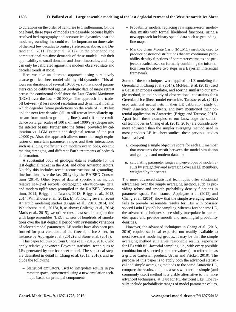
5. GL2D: past grounding-line locations (see Fig. 1). Only
the Amundsen Sea region is used in this study. Misfit
M5: based on model–data mismatches for 20, 15, 10,
and 5 ka. Data: RAISED Consortium (2014) (Anderson
et al., 2014; Hillenbrand et al., 2014; Larter et al., 2014;
Mackintosh et al., 2014; O Cofaigh et al., 2014).
6. RSL: past relative sea-level (RSL) records. Misfit M6:
based on a χ -squared measure of model–data differ-
ences at individual sites. Data: compilation in Briggs
and Tarasov (2013).
7. ELEV/DSURF: past cosmogenic elevation vs. age
(ELEV) and thickness vs. age (DSURF). Misfits M7a,
M7b: based on model–data differences at individual
sites, combined as in Appendix B. Data: compilations
in Briggs and Tarasov (2013) for ELEV; in RAISED
Consortium (2014) with individual citations as above
for DSURF.
8. UPL: modern uplift rates on rock outcrops. Misfit M8:
based on model–data difference at individual sites.
Data: compilation in Whitehouse et al. (2012b).
2.4 Combination into one aggregate score for a simple
averaging method
Each of the misfits above are first transformed into a normal-
ized individual score for each data type i = 1 to 8. The trans-
formations differ for the two approaches mentioned above.
Geosci. Model Dev., 9, 1697–1723, 2016 www.geosci-model-dev.net/9/1697/2016/
D. Pollard et al.: Large ensemble modeling of the last deglacial retreat of the West Antarctic Ice Sheet 1701
Figure 1. Geographical map of West Antarctica. Light yellow
shows the modern extent of grounded ice (using Bedmap2 data;
Fretwell et al., 2013). Blue and purple areas show expanded
grounded-ice extents at 5, 10, 15 and 20 ka (thousands of years
before present) reconstructed by the RAISED Consortium (2014),
plotted using their vertex information (S. Jamieson, personl com-
munication, 2015), and choosing their Scenario A for the Weddell
embayment (Hillenbrand et al., 2014). These maps are used in the
large ensemble scoring (TOTE, TROUGH and GL2D data types,
Sect. 2.3).
2.4.1 For approach (a), closely following Gaussian
error forms, using misfits Mi as described in
Appendix B
– For a given data type i, the misfits Mi for all runs (1 to
625) are sorted, and normalized using the median value
M50i , i.e., M ′i =Mi / M50
i . This is somewhat analogous
to the heuristic scaling for overall scores in Briggs et
al. (2014, their Sect. 2.3), but applied here to individual
types.
– The individual score Si for data type i and each run is
set to e−M′i .
– The aggregate score for each run is S =
S1S2S3S4S5S6S7S8, i.e., e−6M′i .
Of the two approaches, this most closely follows Briggs and
Tarasov (2013) and Briggs et al. (2014), except for their inter-
data-type weighting, which assigns very different weights to
the individual types based on spatial and temporal volumes of
influence (Briggs and Tarasov, 2013, their Sect. 4.3.2; Briggs
et al., 2014, their Sect. 2.2). Here, we assume that each data
type is of equal importance to the overall score, and that if
any one individual score is very bad (Si ≈ 0), the overall
score S should also be ≈ 0. This corresponds to the notion
that if any single data type is completely mismatched, the
run should be rejected as unrealistic, regardless of the fit to
the other data types. The fits to past data, even if more uncer-
tain and sparser than modern, seem equally important to the
goal of obtaining the best calibration for future applications
with very large departures from modern conditions.
2.4.2 For the more heuristic approach (b), using misfits
Mi as described in Appendix B
– For a given data type i, a “cutoff” value Ci is set by
taking the geometric mean (i.e., square root of the prod-
uct) of (i) the minimum (best) misfits Mi over all runs
1 to 625, and (ii) the algebraic average of the 10 largest
(worst) values. The 10 worst values are used to avoid a
single outlier that could be unbounded; the single best
value is used because it is bounded by zero, and is not
an outlier but represents close-to-the-best possible sim-
ulation with the current model. The geometric mean and
not the algebraic mean of these two numbers is more ap-
propriate if the values range over many orders of mag-
nitude.
– The normalized misfit M ′i for data type i and each run
is set to Mi/Ci . We implicitly assume that M ′i values
close to 0 (Mi � Ci) represent very good simulations
of this data type, close to the best possible within the
LE. M ′i values ≥ 1 (Mi ≥ Ci) represent very poor sim-
ulations, diverging from this data type so much that the
run should be rejected no matter what the other scores
are.
– The individual score Si for data type i and each run is
set to max [0,1−M ′i ].
– The aggregate score for each run is S =
(S1S2S3S4S5S6S7S8)1/8.
In both approaches, the formulae apply equal weights to
the individual data types, and do not use “inter-data-type”
weighting (Briggs and Tarasov, 2013; Briggs et al., 2014).
As in (a), if any individual score Si is ≈ 0, then the over-
all score S is ≈ 0, and the discussion above also applies to
approach (b). Both approaches have loose links to the cal-
ibration technique in Gladstone et al. (2012) and the more
formal treatment in McNeall et al. (2013).
2.5 Advanced statistical techniques
The more advanced statistical techniques (Chang et al., 2015,
2016) consist of an emulation and a calibration stage, involv-
ing the same four model parameters and the 625-member
LE as above. The aggregate scores S described in Sect. 2.4
are not used at all. The techniques are outlined here; full ac-
counts are given in Chang et al. (2015, 2016).
2.5.1 Emulation phase
Emulation is the statistical approach by which a computer
model is approximated by a statistical model. This statistical
www.geosci-model-dev.net/9/1697/2016/ Geosci. Model Dev., 9, 1697–1723, 2016
1702 D. Pollard et al.: Large ensemble modeling of the last deglacial retreat of the West Antarctic Ice Sheet
approximation is obtained by running the model at many pa-
rameter settings and then “fitting” a Gaussian process model
to the input–output combinations, analogous to fitting a re-
gression model that relates independent variables (parame-
ters) to dependent variables (model output) in order to make
predictions of the dependent variable at new values of the
independent variables. Of course, unlike basic regression,
the model output may itself be multivariate. An emulator is
useful because (i) it provides a computationally inexpensive
method for approximating the output of a computer model
at any parameter setting without having to actually run the
model each time, and (ii) it provides a statistical model relat-
ing parameter values to computer model output – this means
the approximations automatically include uncertainties, with
larger uncertainties at parameter settings that are far from pa-
rameter values where the computer model has already been
run. Specifically, the model output consisting of (i) mod-
ern grounding-line maps, and (ii) past locations of ground-
ing lines vs. time along the centerline trough of Pine Island,
are first reduced in dimensionality by computing principal
components (PCs) over all LE runs. (Principal components
are often referred to in the atmospheric science literature as
empirical orthogonal functions or EOFs.) The first 10 PCs
are used for modern maps, and the first 20 for past trough
locations. Hence, we develop a Gaussian process emulator
for each of the above PCs. Gaussian process emulators work
especially well for model outputs that are scalars. The em-
ulators are “fitted” to the PCs using a maximum likelihood
estimation-based approach developed in Chang et al. (2015)
that addresses the complications that arise due to the fact that
the data are non-Gaussian. Details are available in Chang et
al. (2015, 2016). The emulators provide a statistical model
that essentially replaces the data types TOTE, TROUGH and
GL2D described in Sect. 2.3.
In an extension to Chang et al. (2016), Gaussian pro-
cess emulators are also used here to estimate distributions
of individual score values for the five data types TOTI,
TOTDH, RSL, ELEV/DSURF and UPL (S2, S3, S6, S7, S8,
approach (b), Sect. 2.3 and Appendix B), one emulator per
score. Again, emulators are developed for each of the scores
by using the Gaussian process machinery and maximum like-
lihood estimation.
2.5.2 Calibration phase
The calibration stage solves the following problem in a statis-
tically rigorous fashion: given observations and model runs
at various parameter settings, which parameters of the model
are most likely? In a Bayesian inferential framework, this
translates to learning about the posterior probability distribu-
tion of the parameter values given all the available computer
model runs and observations. The approach may be sketched
out as follows. The emulation phase provides a statistical
model connecting the parameters to the model output. Sup-
pose it is assumed that the model at a particular (ideal) set of
parameter values produces output that resembles the observa-
tions of the process. We also allow for measurement error and
systematic discrepancies between the computer model and
the real physical system. We do this via a “discrepancy func-
tion” that simultaneously accounts for both; this is reasonable
because both sources of error are important while also being
difficult to tease apart. Hence, one can think of our approach
as assuming that the observations are modeled as the model
output at an ideal parameter setting, added to a discrepancy
function. Once we are able to specify a model in this fashion,
Bayesian inference provides a a very standard approach to
obtain the resulting posterior distribution of the parameters:
we start with a prior distribution for the parameters, where we
assume that all the values are equally likely before any obser-
vations are obtained, and then use Bayes’ theorem to find the
posterior distribution given the data. The posterior distribu-
tion cannot be found in analytical form. Hence, in this second
“calibration” stage, posterior densities of the model param-
eters are inferred via Markov chain Monte Carlo (MCMC).
The observation and model quantities used in emulation and
calibration consist of the modern and past grounding-line lo-
cations, and five individual scores. The discrepancy function
is accounted for in assessing model vs. observed grounding-
line fits in our Bayesian approach. It is based in part on the lo-
cations and times in which grounded ice occurs in the model
and not in the observations, or vice versa, in 50 % or more
of the LE runs (Chang et al., 2015, 2016). For the individ-
ual scores, we use exponential marginal densities, whose rate
parameters receive gamma priors scaled in such a way that
the 90th percentile of the prior density coincides with each
score’s cutoff value Ci in Sect. 2.4.2.
In the above procedures, observational error enters for the
individual scores RSL, ELEV/DSURF and UPL via the cal-
culations described in Appendix B. It is implicitly taken into
account by the discrepancy function for grounding-line loca-
tions. Observational error is considered to be negligible for
modern TOTI and TOTDH scores.
3 Results: aggregate scores with a simple
averaging method
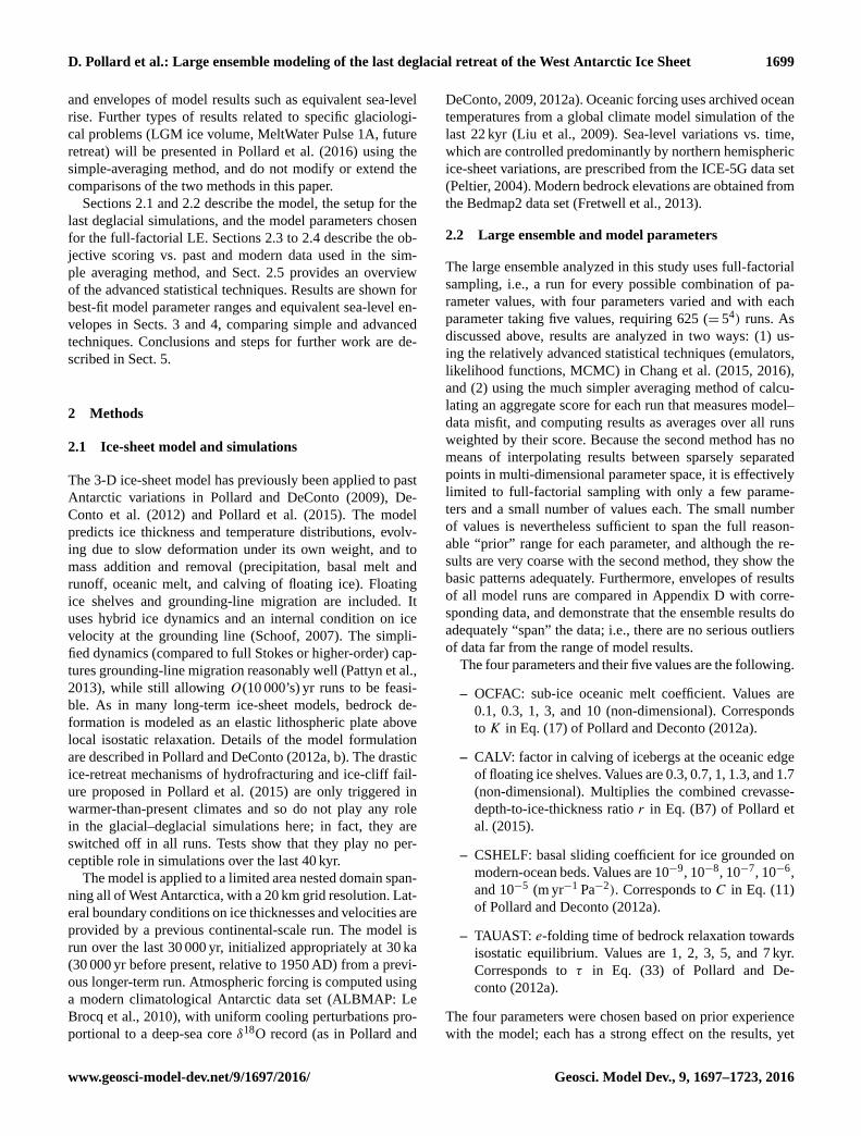
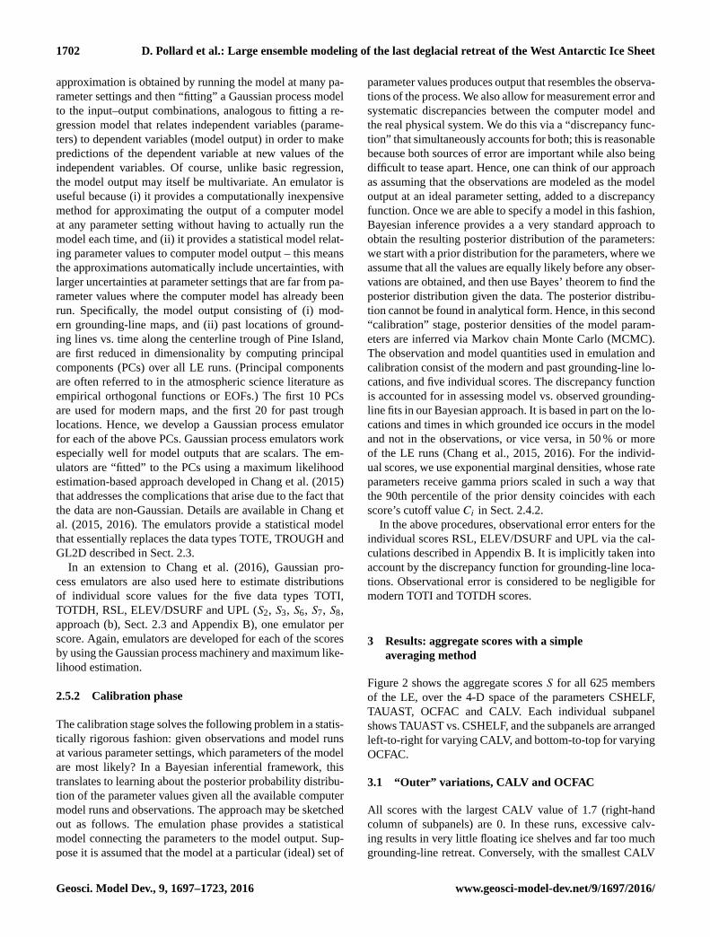
Figure 2 shows the aggregate scores S for all 625 members
of the LE, over the 4-D space of the parameters CSHELF,
TAUAST, OCFAC and CALV. Each individual subpanel
shows TAUAST vs. CSHELF, and the subpanels are arranged
left-to-right for varying CALV, and bottom-to-top for varying
OCFAC.
3.1 “Outer” variations, CALV and OCFAC
All scores with the largest CALV value of 1.7 (right-hand
column of subpanels) are 0. In these runs, excessive calv-
ing results in very little floating ice shelves and far too much
grounding-line retreat. Conversely, with the smallest CALV
Geosci. Model Dev., 9, 1697–1723, 2016 www.geosci-model-dev.net/9/1697/2016/
D. Pollard et al.: Large ensemble modeling of the last deglacial retreat of the West Antarctic Ice Sheet 1703
Figure 2. Aggregate scores for the complete large ensemble suite of
runs (625 runs, 4 model parameters, 5 values each, Sect. 2.2), used
in the simple method with score-weighted averaging. The score val-
ues range from 0 (white, no skill) to 100 (dark red, perfect fit). The
figure is organized to show the scores in the 4-D space of parame-
ter variations. The four parameters are CSHELF= basal sliding co-
efficient in modern oceanic areas (exponent x, 10−x m a−1 Pa−2),
TAUAST= e-folding time of bedrock-elevation isostatic relaxation
(kyr), OCFAC= oceanic-melt-rate coefficient at the base of float-
ing ice shelves (non-dimensional) and CALV= calving-rate factor
at the edge of floating ice shelves (non-dimensional). Since each
parameter only takes five values, the results are blocky, but effec-
tively show the behavior of the score over the full range of plausible
parameter values.
value of 0.3 (left-hand column of subpanels), most runs have
too much floating ice and too advanced grounding lines dur-
ing the runs, so most of this column also has zero scores.
However, small CALV can be partially compensated for by
large OCFAC (strong ocean melting), so there are some non-
zero scores in the upper-left subpanels.
3.2 “Inner” variations, CSHELF and TAUAST
For mid-range CALV and OCFAC (subpanels near the cen-
ter of the figure), the best scores require high CSHELF (inner
x axis) values, i.e., slippery ocean-bed coefficients of 10−6 to
10−5 m a−1 Pa−2. This is the most prominent signal in Fig. 2,
and is consistent with the widespread extent of deformable
sediments on continental shelves noted above. Ideally the
LE should have included CSHELF values greater than 10−5.
However, we note that values of 10−5 to 10−6 have been
found to well represent active Siple Coast ice-stream beds
in model inversions (Pollard and DeConto, 2012b). Subse-
quent work with wider CSHELF ranges confirms that values
around 10−5 are in fact optimal, with unrealistic behavior for
larger values (Pollard et al., 2016).
Somewhat lower but still reasonable scores exist for lower
CSHELF values of 10−7, but only for higher OCFAC (3 to
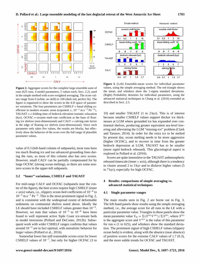
Figure 3. (Left) Ensemble-mean scores for individual parameter
values, using the simple averaging method. The red triangle shows
the mean, and whiskers show the 1-sigma standard deviations.
(Right) Probability densities for individual parameters, using the
advanced statistical techniques in Chang et al. (2016) extended as
described in Sect. 2.5.
10) and smaller TAUAST (1 to 2 kyr). This is of interest
because smaller CSHELF values support thicker ice thick-
nesses at LGM where grounded ice has expanded over con-
tinental shelves, producing greater equivalent sea-level low-
ering and alleviating the LGM “missing-ice” problem (Clark
and Tarasov, 2014). In order for the extra ice to be melted
by present day, ocean melting needs to be more aggressive
(higher OCFAC), and to recover in time from the greater
bedrock depression at LGM, TAUAST has to be smaller
(more rapid bedrock rebound). This glaciological aspect is
explored in Pollard et al. (2016).
Scores are quite insensitive to the TAUAST asthenospheric
rebound timescale (inner y axis), although there is a tendency
to cluster around 2 to 3 kyr and to disfavor higher values (5
to 7 kyr), especially for high OCFAC.
4 Results: comparisons of simple averaging vs.
advanced statistical techniques
4.1 Single parameter ranges
The main results seen in Fig. 2 are borne out in Fig. 3.
The left-hand panels show results using the simple averaging
method, i.e., the average score for all runs in the LE with a
particular parameter value. Triangles in these panels show the
mean parameter value Vm =6(S(n)V (n))/6S(n), where S(n)
is the aggregate score and V (n) is the value of this parameter
for run n (1 to 625), and whiskers show the standard devia-
tion. The prominent signal of high CSHELF values (slippery
ocean beds) is evident, along with the absence (near absence)
of positive scores for the extreme CALV values of 1.7 (0.3),
and the more subtle trends for OCFAC and TAUAST.
www.geosci-model-dev.net/9/1697/2016/ Geosci. Model Dev., 9, 1697–1723, 2016
1704 D. Pollard et al.: Large ensemble modeling of the last deglacial retreat of the West Antarctic Ice Sheet
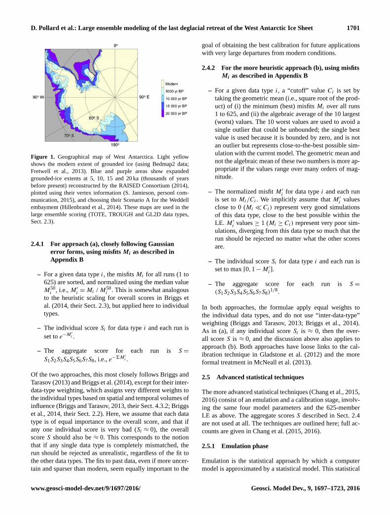
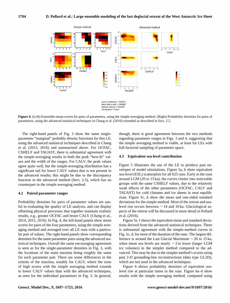
Figure 4. (Left) Ensemble-mean scores for pairs of parameters, using the simple averaging method. (Right) Probability densities for pairs of
parameters, using the advanced statistical techniques in Chang et al. (2016) extended as described in Sect. 2.5.
The right-hand panels of Fig. 3 show the same single-
parameter “marginal” probably density functions for this LE,
using the advanced statistical techniques described in Chang
et al. (2015, 2016) and summarized above. For OCFAC,
CSHELF and TAUAST, there is substantial agreement with
the simple-averaging results in both the peak “best-fit” val-
ues and the width of the ranges. For CALV, the peak values
agree quite well, but the simple-averaging distribution has a
significant tail for lower CALV values that is not present in
the advanced results; this might be due to the discrepancy
function in the advanced method (Sect. 2.5), which has no
counterpart in the simple averaging method.
4.2 Paired parameter ranges
Probability densities for pairs of parameter values are use-
ful in evaluating the quality of LE analysis, and can display
offsetting physical processes that together maintain realistic
results, e.g., greater OCFAC and lesser CALV (Chang et al.,
2014, 2015, 2016). In Fig. 4, the left-hand panels show mean
scores for pairs of the four parameters, using the simple aver-
aging method and averaged over all LE runs with a particu-
lar pair of values. The right-hand panels show corresponding
densities for the same parameter pairs using the advanced sta-
tistical techniques. Overall the same encouraging agreement
is seen as for the single-parameter densities in Fig. 3, with
the locations of the main maxima being roughly the same
for each parameter pair. There are some differences in the
extents of the maxima, notably for CALV, where the zone
of high scores with the simple averaging method extends
to lower CALV values than with the advanced techniques,
as seen for the individual parameters in Fig. 3. In general,
though, there is good agreement between the two methods
regarding parameter ranges in Figs. 3 and 4, suggesting that
the simple averaging method is viable, at least for LEs with
full-factorial sampling of parameter space.
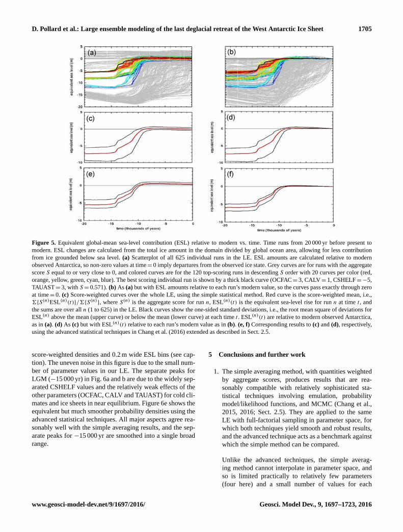
4.3 Equivalent sea-level contribution
Figure 5 illustrates the use of the LE to produce past en-
velopes of model simulations. Figure 5a, b show equivalent
sea-level (ESL) scatterplots for all 625 runs. Early in the runs
around LGM (20 to 15 ka), the curves cluster into noticeable
groups with the same CSHELF values, due to the relatively
weak effects of the other parameters (OCFAC, CALV and
TAUAST) for cold climates and ice sheets in near equilib-
rium. Figure 5c, d show the mean and one-sided standard
deviations for the simple method. Most of the retreat and sea-
level rise occurs between ∼ 14 and 10 ka. Glaciological as-
pects of the retreat will be discussed in more detail in Pollard
et al. (2016).
Figure 5e, f shows the equivalent mean and standard devia-
tions derived from the advanced statistical techniques. There
is substantial agreement with the simple-method curves in
Fig. 5c, d, for most of the duration of the runs. The largest dif-
ference is around the Last Glacial Maximum ∼ 20 to 15 ka,
when mean sea levels are nearly ∼ 2 m lower (larger LGM
ice volumes) in the simpler method compared to the ad-
vanced. This may be due to the simpler method’s scores using
past 2-D grounding-line reconstructions (data type GL2D),
which are not used in the advanced techniques.
Figure 6 shows probability densities of equivalent sea-
level rise at particular times in the runs. Figure 6a–d show
results with the simple averaging method, computed using
Geosci. Model Dev., 9, 1697–1723, 2016 www.geosci-model-dev.net/9/1697/2016/
D. Pollard et al.: Large ensemble modeling of the last deglacial retreat of the West Antarctic Ice Sheet 1705
Figure 5. Equivalent global-mean sea-level contribution (ESL) relative to modern vs. time. Time runs from 20 000 yr before present to
modern. ESL changes are calculated from the total ice amount in the domain divided by global ocean area, allowing for less contribution
from ice grounded below sea level. (a) Scatterplot of all 625 individual runs in the LE. ESL amounts are calculated relative to modern
observed Antarctica, so non-zero values at time= 0 imply departures from the observed ice state. Grey curves are for runs with the aggregate
score S equal to or very close to 0, and colored curves are for the 120 top-scoring runs in descending S order with 20 curves per color (red,
orange, yellow, green, cyan, blue). The best scoring individual run is shown by a thick black curve (OCFAC= 3, CALV= 1, CSHELF=−5,
TAUAST= 3, with S= 0.571). (b) As (a) but with ESL amounts relative to each run’s modern value, so the curves pass exactly through zero
at time= 0. (c) Score-weighted curves over the whole LE, using the simple statistical method. Red curve is the score-weighted mean, i.e.,
6{S(n)ESL(n)(t)}/6{S(n)}, where S(n) is the aggregate score for run n, ESL(n)(t) is the equivalent sea-level rise for run n at time t , and
the sums are over all n (1 to 625) in the LE. Black curves show the one-sided standard deviations, i.e., the root mean square of deviations for
ESL(n) above the mean (upper curve) or below the mean (lower curve) at each time t . ESL(n)(t) are relative to modern observed Antarctica,
as in (a). (d) As (c) but with ESL(n)(t) relative to each run’s modern value as in (b). (e, f) Corresponding results to (c) and (d), respectively,
using the advanced statistical techniques in Chang et al. (2016) extended as described in Sect. 2.5.
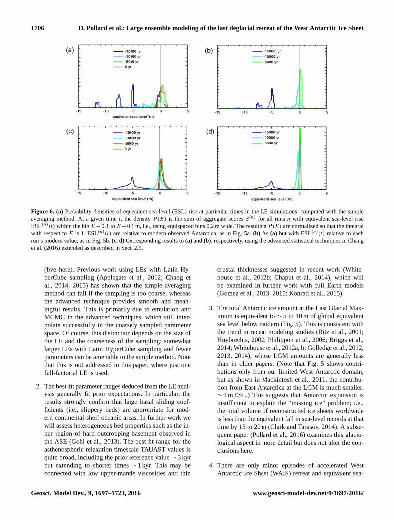
score-weighted densities and 0.2 m wide ESL bins (see cap-
tion). The uneven noise in this figure is due to the small num-
ber of parameter values in our LE. The separate peaks for
LGM (−15 000 yr) in Fig. 6a and b are due to the widely sep-
arated CSHELF values and the relatively weak effects of the
other parameters (OCFAC, CALV and TAUAST) for cold cli-
mates and ice sheets in near equilibrium. Figure 6e shows the
equivalent but much smoother probability densities using the
advanced statistical techniques. All major aspects agree rea-
sonably well with the simple averaging results, and the sep-
arate peaks for −15 000 yr are smoothed into a single broad
range.
5 Conclusions and further work
1. The simple averaging method, with quantities weighted
by aggregate scores, produces results that are rea-
sonably compatible with relatively sophisticated sta-
tistical techniques involving emulation, probability
model/likelihood functions, and MCMC (Chang et al.,
2015, 2016; Sect. 2.5). They are applied to the same
LE with full-factorial sampling in parameter space, for
which both techniques yield smooth and robust results,
and the advanced technique acts as a benchmark against
which the simple method can be compared.
Unlike the advanced techniques, the simple averag-
ing method cannot interpolate in parameter space, and
so is limited practically to relatively few parameters
(four here) and a small number of values for each
www.geosci-model-dev.net/9/1697/2016/ Geosci. Model Dev., 9, 1697–1723, 2016
1706 D. Pollard et al.: Large ensemble modeling of the last deglacial retreat of the West Antarctic Ice Sheet
Figure 6. (a) Probability densities of equivalent sea-level (ESL) rise at particular times in the LE simulations, computed with the simple
averaging method. At a given time t , the density P(E) is the sum of aggregate scores S(n) for all runs n with equivalent sea-level rise
ESL(n)(t) within the bin E−0.1 to E+0.1 m, i.e., using equispaced bins 0.2 m wide. The resulting P(E) are normalized so that the integral
with respect to E is 1. ESL(n)(t) are relative to modern observed Antarctica, as in Fig. 5a. (b) As (a) but with ESL(n)(t) relative to each
run’s modern value, as in Fig. 5b. (c, d) Corresponding results to (a) and (b), respectively, using the advanced statistical techniques in Chang
et al. (2016) extended as described in Sect. 2.5.
(five here). Previous work using LEs with Latin Hy-
perCube sampling (Applegate et al., 2012; Chang et
al., 2014, 2015) has shown that the simple averaging
method can fail if the sampling is too coarse, whereas
the advanced technique provides smooth and mean-
ingful results. This is primarily due to emulation and
MCMC in the advanced techniques, which still inter-
polate successfully in the coarsely sampled parameter
space. Of course, this distinction depends on the size of
the LE and the coarseness of the sampling; somewhat
larger LEs with Latin HyperCube sampling and fewer
parameters can be amenable to the simple method. Note
that this is not addressed in this paper, where just one
full-factorial LE is used.
2. The best-fit parameter ranges deduced from the LE anal-
ysis generally fit prior expectations. In particular, the
results strongly confirm that large basal sliding coef-
ficients (i.e., slippery beds) are appropriate for mod-
ern continental-shelf oceanic areas. In further work we
will assess heterogeneous bed properties such as the in-
ner region of hard outcropping basement observed in
the ASE (Gohl et al., 2013). The best-fit range for the
asthenospheric relaxation timescale TAUAST values is
quite broad, including the prior reference value ∼ 3 kyr
but extending to shorter times ∼ 1 kyr. This may be
connected with low upper-mantle viscosities and thin
crustal thicknesses suggested in recent work (White-
house et al., 2012b; Chaput et al., 2014), which will
be examined in further work with full Earth models
(Gomez et al., 2013, 2015; Konrad et al., 2015).
3. The total Antarctic ice amount at the Last Glacial Max-
imum is equivalent to ∼ 5 to 10 m of global equivalent
sea level below modern (Fig. 5). This is consistent with
the trend in recent modeling studies (Ritz et al., 2001;
Huybrechts, 2002; Philippon et al., 2006; Briggs et al.,
2014; Whitehouse et al., 2012a, b; Golledge et al., 2012,
2013, 2014), whose LGM amounts are generally less
than in older papers. (Note that Fig. 5 shows contri-
butions only from our limited West Antarctic domain,
but as shown in Mackintosh et al., 2011, the contribu-
tion from East Antarctica at the LGM is much smaller,
∼ 1 m ESL.) This suggests that Antarctic expansion is
insufficient to explain the “missing ice” problem; i.e.,
the total volume of reconstructed ice sheets worldwide
is less than the equivalent fall in sea-level records at that
time by 15 to 20 m (Clark and Tarasov, 2014). A subse-
quent paper (Pollard et al., 2016) examines this glacio-
logical aspect in more detail but does not alter the con-
clusions here.
4. There are only minor episodes of accelerated West
Antarctic Ice Sheet (WAIS) retreat and equivalent sea-
Geosci. Model Dev., 9, 1697–1723, 2016 www.geosci-model-dev.net/9/1697/2016/
D. Pollard et al.: Large ensemble modeling of the last deglacial retreat of the West Antarctic Ice Sheet 1707
level rise in the simulations (Fig. 5), and none with
magnitudes comparable to Melt Water Pulse 1A for
instance, with ∼ 15 m ESL rise in ∼ 350 yr around
∼ 14.5 ka (Deschamps et al., 2012), in apparent con-
flict with significant Antarctic contribution implied by
sea-level fingerprinting studies (Bassett et al., 2005; De-
schamps et al., 2012) and ice-rafted debris (IRD) core
analysis (Weber et al., 2014). Model retreat rates are
examined in more detail in Pollard et al. (2016), again
without altering the findings here.
A natural extension of this work is to extend the Antarc-
tic model simulations and LE methods into the future, using
climates and ocean warming following Representative Con-
centration Pathway scenarios (Meinshausen et al., 2011). In
these warmer climates we expect marine ice-sheet instabil-
ity to occur in WAIS basins, consistent with past retreats
simulated in Pollard and DeConto (2009). Also, drastic re-
treat mechanisms of hydrofracture and ice-cliff failure, not
triggered in the colder-than-present simulations of this pa-
per, may play a role, as found for the Pliocene in Pollard et
al. (2015). Future applications with simple-average LEs are
described in Pollard et al. (2016), and detailed future scenar-
ios with another type of LE are described in DeConto and
Pollard (2016).
Code availability
The code for the ice-sheet model (PSUICE-3D) is avail-
able on request from the corresponding author. The post-
processing codes for the large-ensemble statistical analyses
are highly tailored to specific sets of model output and are
not made available; however, modules that compute scores
for the individual data types are also available on request.
www.geosci-model-dev.net/9/1697/2016/ Geosci. Model Dev., 9, 1697–1723, 2016
1708 D. Pollard et al.: Large ensemble modeling of the last deglacial retreat of the West Antarctic Ice Sheet
Appendix A: Model parameters varied in the
large ensemble
The four model parameters (OCFAC, CALV, CSHELF and
TAUAST) and their ranges in the large ensemble are sum-
marized in Sect. 2.2. Their physical effects in the model and
associated uncertainties are discussed in more detail here.
OCFAC is the main coefficient in the parameterization
of sub-ice-shelf oceanic melt, which is proportional to the
square of the difference between nearby water temperature at
400 m and the pressure-melting point of ice. Oceanic melt-
ing (or freezing) erodes (or grows on) the base of float-
ing ice shelves, as warm waters at intermediate depths flow
into the cavities below the shelves. The resulting ice-shelf
thinning reduces pinning points and lateral friction, and
thus back stress on grounded interior ice. As mentioned
above, recent increases in ocean melt rates are considered
to be the main cause of ongoing downdraw and accelera-
tion of interior ice in the ASE sector of WAIS (Pritchard et
al., 2012; Dutrieux et al., 2014). High-resolution dynamical
ocean models (Hellmer et al., 2012) are not yet practical on
these timescales, and simple parameterizations of sub-ice-
shelf melting such as the one used here are quite uncertain
(e.g., Holland et al., 2008). For small (large) OCFAC values,
oceanic melting is reduced (increased), ice shelves thicken
(thin), discharge of interior ice across the grounding line de-
creases (increases), and grounding lines tend to advance (re-
treat).
CALV is the main factor in the parameterization of ice-
berg calving at the oceanic edges of floating shelves. Calv-
ing has important effects on ice-shelf extent with strong feed-
back effects via buttressing of interior ice. However, the pro-
cesses controlling calving are not well understood, probably
depending on a combination of pre-existing fracture regime,
large-scale stresses, and hydrofracturing by surface meltwa-
ter. There is little consensus on calving parameterizations.
We use a common approach based on parameterized crevasse
depths and their ratio to ice thickness (Benn et al., 2007; Nick
et al., 2010). For small (large) CALV, calving is decreased
(increased), producing more (less) extensive floating shelves,
and greater (lesser) buttressing of interior ice.
CSHELF is the basal sliding coefficient for ice grounded
on areas that are ocean bed today (and is not frozen to the
bed). Coefficients under modern grounded ice are deduced by
inverse methods (Pollard and DeConto, 2012b; Morlighem et
al., 2013), but they are relatively unconstrained for modern
oceanic beds, across which grounded ice advanced at the Last
Glacial Maximum ∼ 20 to 15 ka. Most oceanic beds around
Antarctica are covered in deformable sediment today, due to
Holocene marine sedimentation, and to earlier transport and
deposition of till by previous ice advances. For these regions,
coefficients are expected to be relatively high (i.e., slippery
bed), but there is still a plausible range that has significant ef-
fects on model results, because it strongly controls the steep-
ness of the ice-sheet surface profile and ice thicknesses, and
thus the sensitivity to climate change. In this paper, we vary
the sliding coefficient CSHELF uniformly for all modern-
oceanic areas. (In further work, we will allow for heterogene-
ity such as the hard crystalline bedrock zone observed in the
inner Amundsen Sea Embayment; Gohl et al., 2013).
TAUAST is the e-folding time of asthenosephic relaxation
in the bedrock model component. Ice-sheet evolution on long
timescales is affected quite strongly by the bedrock response
to varying ice loads, especially for marine ice sheets in con-
tact with the ocean where bathymetry determines grounding-
line depths. During deglacial retreat, the bedrock rebounds
upwards due to reduced ice load, which slows down ice re-
treat due to shallower grounding-line depths and less dis-
charge of interior ice. However, theO(103) yr lag in this pro-
cess is important in reducing this negative feedback, and ac-
celerates the positive feedback of marine ice-sheet instabil-
ity if the bed deepens into the ice-sheet interior. As in many
large-scale ice-sheet models, our bedrock response is repre-
sented by a simple Earth model consisting of an elastic plate
over a local e-folding relaxation towards isostatic equilib-
rium (elastic lithosphere relaxing asthenosphere). Based on
more sophisticated global Earth models, the asthenospheric
e-folding timescale is commonly set to 3 kyr (e.g., Gomez et
al., 2013), but note that recent geophysical studies suggest
considerably shorter timescales for some West Antarctic re-
gions (Whitehouse et al., 2012b; Chaput et al., 2014). In fur-
ther work we plan to perform large ensembles with the ice-
sheet model coupled to a full Earth model, extending Gomez
et al. (2013, 2015).
Geosci. Model Dev., 9, 1697–1723, 2016 www.geosci-model-dev.net/9/1697/2016/
D. Pollard et al.: Large ensemble modeling of the last deglacial retreat of the West Antarctic Ice Sheet 1709
Appendix B: Data types and individual misfits
The eight types of modern and past data used in evaluating
the model simulations are summarized in Sect. 2.3. More de-
tails on the algorithms used to compute the individual mis-
matches M1 to M8 with model quantities are given below.
The term “domain” refers to the nested model grid that spans
all of West Antarctica, and we only compare with observa-
tional sites and data within this domain. Modern observed
data are from the Bedmap2 data set (Fretwell et al., 2013).
As discussed in Sects. 2.3 and 2.4, we use 2 approaches
in scoring: (a) more closely following Gaussian error forms,
and (b) with more heuristic forms. Some of the algorithms
for individual misfits differ between the two, as indicated by
bullets (a) and (b) below. For most data types, approach (a)
uses mean-square errors, and (b) uses root-mean-square er-
rors. For some data types, the errors are normalized not by
observational uncertainty, but by an “acceptable model er-
ror magnitude” representing typical model departures from
observations in reasonably realistic runs, if this is larger than
observational error. Note that if this scaling uncertainty is the
same for all data of a given type, it cancels out in the normal-
ization of individual misfits (Mi to Mi ′ in Sect. 2.4), so has
no effect on the further results.
B1 TOTE
Modern grounding-line locations.
A′= total area of mismatch where model is grounded and
observed is floating ice or ocean, or vice versa. Atot= total
area of the domain.
Approach (a): Misfit M1 = (A′/B)2, where
B = (Atot)1/2σw. Here B is the product of the linear
domain size, and σw = 30 km representing the typical size
of modern grounding-line location errors in “reasonable”
model runs.
Approach (b): Misfit M1 = A′/Atot.
B2 TOTI
Modern floating ice-shelf locations.
A′= total area of mismatch where model has floating ice
and observed does not, or vice versa. Atot= total area of the
domain.
Approach (a): Misfit M1 = (A′/B)2, where
B = (Atot)1/2σw. Here B is the product of the linear
domain size, and σw = 30 km representing the typical size
of modern floating-ice extent errors in “reasonable” model
runs.
Approach (b): Misfit M1 = A′/Atot
B3 TOTDH
Modern grounded ice thicknesses.
Approach (a): Misfit M3 is the mean of ((h−hobs)/σh)2,
where h is model ice thickness, hobs is observed ice thick-
ness, and σh = 10 m represents the typical size of modern
ice thickness errors in “reasonable” model runs. The mean is
taken over areas with observed modern grounded ice.
Approach (b): Misfit M3 is the root mean square of (h−
hobs), over areas with observed modern grounded ice.
B4 TROUGH
Past grounding-line distance vs. time along centerline
troughs of Pine Island Glacier, and optionally the Ross and
Weddell basins. Observed distances at ages 20, 15, 10 and
5 ka are obtained from grounding-line reconstructions of the
RAISED Consortium (2014): Anderson et al. (2014) for the
Ross; Larter et al. (2014) for the Amundsen Sea, and Hillen-
brand et al. (2014) for the Weddell, using their Scenario A of
most retreated Weddell ice. Distances are then linearly inter-
polated in time between these dates. The centerline trough for
Pine Island Glacier is extended across the continental shelf
following the paleo-ice-stream trough shown in Jakobsson et
al. (2011). The resulting Pine Island Glacier transect vs. time
is similar to that in Smith et al. (2014).
Approach (a): Misfit M4 is the mean of ((x− xobs)/σx)2,
where x is model grounding-line position on the transect at
a given time, xobs is the reconstructed position, and σx =
30 km represents a typical difference in “reasonable” model
runs, and is also midway between “measured” and “inferred”
uncertainties in the reconstructed data (RAISED Consor-
tium, 2014). The mean is taken over the period 20 to 0 ka.
Approach (b): Misfit M4 is the root-mean-square of (x−
xobs), over the period 20 to 0 ka.
In this study just the Pine Island Glacier trough is used, but
if the Ross and Weddell are used also, the means are taken
over all three troughs.
B5 GL2D
Past grounding-line locations. This uses reconstructed
grounding-line maps for 20, 15, 10, and 5 ka by the RAISED
Consortium (2014; Anderson et al., 2014; Hillenbrand et al.,
2014; Larter et al., 2014; Mackintosh et al., 2014; O Cofaigh
et al., 2014), with vertices provided by S. Jamieson, personal
communication, 2015, and choosing their Scenario A for the
Weddell embayment (Hillenbrand et al., 2014). The modern
grounding line (0 ka) is derived from the Bedmap2 data set
(Fretwell et al., 2013). For this study only the Amundsen Sea
region is considered. We allow for uncertainty in the past re-
constructions by setting a probability of reconstructed float-
ing ice or open ocean at each point Pobs as follows.
i. Computing the distance D1 from the reconstructed
grounding line.
ii. Dividing this distance by the sum D2 of the (Kriged)
reported uncertainty of nearby vertices (interpreting
their “measured”= 10 km, “inferred”= 50 km, “spec-
ulative”= 100 km) and a distance that ramps up to
www.geosci-model-dev.net/9/1697/2016/ Geosci. Model Dev., 9, 1697–1723, 2016
1710 D. Pollard et al.: Large ensemble modeling of the last deglacial retreat of the West Antarctic Ice Sheet
100 km depending on distance to the nearest vertex dv
(i.e., 100 max [0, min [1, (dv− 100)/200]]), to obtain a
scaled distance Ds =D1/D2.
iii. Setting the probability Pobs to a value decaying up-
wards or downwards from 0.5, i.e., to 0.5 e−Ds if on the
grounded side of the grounding line, or to 1–0.5 e−Ds if
on the non-grounded side.
Then the “mismatch probability” Pmis at each model grid
point is set to 2 (0.5−Pobs) if Pobs< 0.5 and the model is
not grounded, or 2 (Pobs−0.5) if Pobs> 0.5 and the model is
grounded. Pmis is zero if the model is not grounded anywhere
on the non-grounded side of the observed grounding line, or
if it is grounded anywhere on the grounded side. Thus, if
the model and observed grounding lines coincide exactly ev-
erywhere, then Pmis is zero at all points, regardless of the
observational uncertainty reflected in Pobs (which seems a
desirable feature).
Approach (a): Misfit M5 is the mean of the squared mis-
match probabilities (Pmis)2, with means computed over 3
separate subdomains: Ross Sea, Amundsen Sea, and Weddell
Sea embayments (defined crudely by intervals of longitude:
150◦ E to 120◦W, 120◦W to 90◦W, and 90◦W to 0, respec-
tively). In this study we only use the mean for the Amundsen
Sea sector. Similarly to TOTE and TOTI, the areal mean is in-
creased by a factor (Atot)1/2/σw, where Atot is the total sub-
domain area and σw = 100 km is a representative width scale
of reasonable past grounding-zone mismatches. Finally, the
mean values for each of the reconstructed past times (20, 15,
10 and 5 ka) are averaged together equally.
Approach (b): Misfit M5 is the mean of Pmis over the
Amundsen Sea sector subdomain, with no adjustment factor
to Atot, and otherwise as for (a) above.
B6 RSL
Past relative sea-level (RSL) records. This uses the compila-
tion by Briggs and Tarasov (2013) of published RSL data vs.
time at sites close to the modern coastline. Following those
authors, the model RSL= [SL(t)−hb(t)]−[SL(0)−hb(0)],
where SL(t) is global sea level (with t = 0 at modern) and
hb is bed elevation, at the closest model grid point to the ob-
served site. The minimum model-minus-observed difference
δRSL for each observed datum is used, i.e., the minimum ele-
vation difference value over all model times within the range
of the observational time uncertainty (tobs± σto).
Approach (a): Misfit M6 is the weighted mean of
(δRSL/σzo)2, where σzo is the observational RSL uncer-
tainty. Just as in Briggs and Tarasov (2013), the default for
σzo is much larger for one-sided constraints (50 m) than ab-
solute constraints (2 m). To reduce the influence of many
nearby (and presumably correlated) data, we closely fol-
low Briggs and Tarasov (2013) and apply “intra-data-type
weighting” in calculating the mean. The weights are in-
versely proportional to the number of measurements within a
distance L of each other, where L is equivalent to 5◦ latitude
(∼ 550 km), so that each∼L-sized cluster of data contributes
∼ equally to the overall mean.
Approach (b): Misfit M6 is the weighted mean of max
[0, |RSL|−σzo]. The uncertainties σzo and the intra-data-type
weights are the same as in (a).
B7 ELEV/DSURF
This uses a combination of two compilations of cosmo-
genic data: elevation vs. age in Briggs and Tarasov (2013)
for ELEV, and thickness change from modern vs. age in
RAISED Consortium (2014) (with individual citations as
above) for DSURF.
For ELEV, the calculations closely follow Briggs and
Tarasov (2013, their Sect. 4.2):
i. a time series of a model ice surface is used, with sea-
level and bedrock elevation changes subtracted out, for
the closest model grid point to each ELEV datum.
ii. Only model elevations with a “deglaciating trend” are
used; i.e., the model elevation for each time is replaced
by the maximum elevation between that time and the
present, if the latter is greater, allowing for an uncer-
tainty 1h=√
2σh, as in Briggs and Tarasov (2013).
iii. The mismatch for each datum is the minimum of
(δh/σh)2+ (δt/σt )
2 over the time series, where δh is
the elevation difference from observed and δt is the time
difference, σh = [σ2hobs+ (100 m)2
]1/2, and σhobs and σt
are the observational uncertainties in elevation and time,
respectively.
Approach (a): Misfit M7 is the weighted mean of the mis-
matches for ELEV above, with intra-data-type weighting ex-
actly as described for RSL above. The DSURF type is not
used in approach (a).
Approach (b): for approach (b), ELEV calculations as
above are combined with DSURF calculations.
The DSURF calculations are simpler: for each datum,
the time series of model surface elevations hs at the clos-
est model grid point is used. The minimum model-minus-
observed difference δhmins is found, i.e., the minimum dif-
ference over all model times within the range of the obser-
vational time uncertainty (tobs± σto). The mismatch for the
datum is max [0,δhmins −σh]where σh is the observational el-
evation uncertainty. The mean over all data is taken, weighted
by intra-data-type weighting as described above. Finally, the
ELEV and DSURF misfits are converted into separate nor-
malized scores (S7a, S7b) as in Sect. 2.4.2, which are then
combined into one individual score S7 = (S7aS7b)1/2.
B8 UPL
This uses modern uplift rates on rock outcrops, using the
compilation in Whitehouse et al. (2012b). For each observed
Geosci. Model Dev., 9, 1697–1723, 2016 www.geosci-model-dev.net/9/1697/2016/

D. Pollard et al.: Large ensemble modeling of the last deglacial retreat of the West Antarctic Ice Sheet 1711
site, the model’s modern ∂hb/∂t at the closest model grid
point is used.
Approach (a): the mismatch at each datum is [(Umod−
Uobs)/σuobs]2, where Umod and Uobs are model and observed
uplift rates, respectively, and σuobs is the observed 1-σ uncer-
tainty. The misfit M8 is the mean over all data points, using
intra-data-type weighting as above.
Approach (b): the mismatch at each datum is (Umod−
Uobs)2, and the misfit M8 is the root-mean square over all
data points, with no intra-data-type weighting (justified by
the relatively uniform distribution of data points).
www.geosci-model-dev.net/9/1697/2016/ Geosci. Model Dev., 9, 1697–1723, 2016
1712 D. Pollard et al.: Large ensemble modeling of the last deglacial retreat of the West Antarctic Ice Sheet
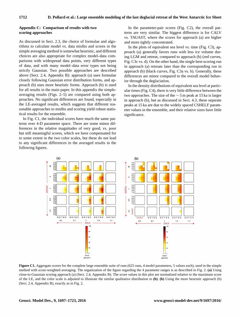
Appendix C: Comparison of results with two
scoring approaches
As discussed in Sect. 2.3, the choice of formulae and algo-
rithms to calculate model vs. data misfits and scores in the
simple averaging method is somewhat heuristic, and different
choices are also appropriate for complex model–data com-
parisons with widespread data points, very different types
of data, and with many model–data error types not being
strictly Gaussian. Two possible approaches are described
above (Sect. 2.4, Appendix B): approach (a) uses formulae
closely following Gaussian error distribution forms, and ap-
proach (b) uses more heuristic forms. Approach (b) is used
for all results in the main paper. In this appendix the simple-
averaging results (Figs. 2–5) are compared using both ap-
proaches. No significant differences are found, especially in
the LE-averaged results, which suggests that different rea-
sonable approaches to misfits and scoring yield robust statis-
tical results for the ensemble.
In Fig. C1, the individual scores have much the same pat-
terns over 4-D parameter space. There are some minor dif-
ferences in the relative magnitudes of very good, vs. poor
but still meaningful scores, which we have compensated for
to some extent in the two color scales, but these do not lead
to any significant differences in the averaged results in the
following figures.
Figure C1. Aggregate scores for the complete large ensemble suite of runs (625 runs, 4 model parameters, 5 values each), used in the simple
method with score-weighted averaging. The organization of the figure regarding the 4 parameter ranges is as described in Fig. 2. (a) Using
close-to-Gaussian scoring approach (a) (Sect. 2.4, Appendix B). The score values in this plot are normalized relative to the maximum score
of the LE, and the color scale is adjusted to illustrate the similar qualitative distribution to (b). (b) Using the more heuristic approach (b)
(Sect. 2.4, Appendix B), exactly as in Fig. 2.
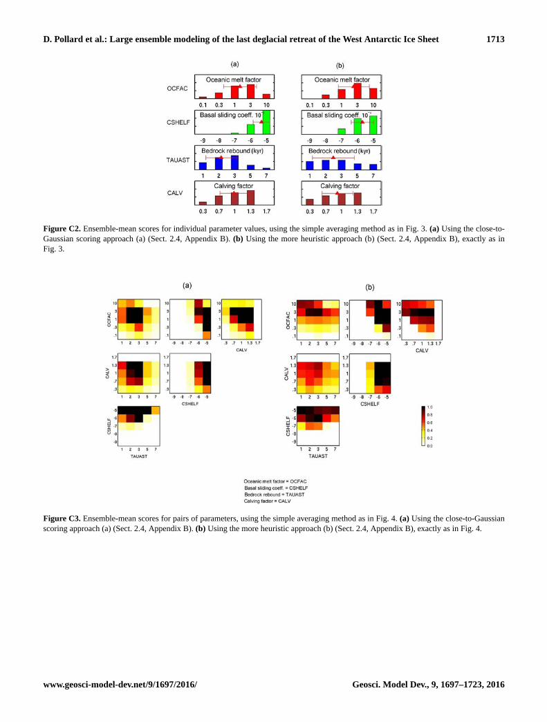
In the parameter-pair scores (Fig. C2), the overall pat-
terns are very similar. The biggest difference is for CALV
vs. TAUAST, where the scores for approach (a) are higher
and more tightly concentrated.
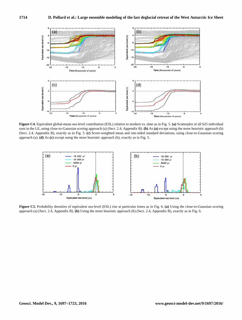
In the plots of equivalent sea level vs. time (Fig. C3), ap-
proach (a) generally favors runs with less ice volume dur-
ing LGM and retreat, compared to approach (b) (red curves,
Fig. C3c vs. d). On the other hand, the single best-scoring run
in approach (a) retreats later than the corresponding run in
approach (b) (black curves, Fig. C3a vs. b). Generally, these
differences are minor compared to the overall model behav-
ior through the deglaciation.
In the density distributions of equivalent sea level at partic-
ular times (Fig. C4), there is very little difference between the
two approaches. The size of the ∼ 5 m peak at 15 ka is larger
in approach (b), but as discussed in Sect. 4.3, these separate
peaks at 15 ka are due to the widely spaced CSHELF param-
eter values in the ensemble, and their relative sizes have little
significance.
Geosci. Model Dev., 9, 1697–1723, 2016 www.geosci-model-dev.net/9/1697/2016/
D. Pollard et al.: Large ensemble modeling of the last deglacial retreat of the West Antarctic Ice Sheet 1713
Figure C2. Ensemble-mean scores for individual parameter values, using the simple averaging method as in Fig. 3. (a) Using the close-to-
Gaussian scoring approach (a) (Sect. 2.4, Appendix B). (b) Using the more heuristic approach (b) (Sect. 2.4, Appendix B), exactly as in
Fig. 3.
Figure C3. Ensemble-mean scores for pairs of parameters, using the simple averaging method as in Fig. 4. (a) Using the close-to-Gaussian
scoring approach (a) (Sect. 2.4, Appendix B). (b) Using the more heuristic approach (b) (Sect. 2.4, Appendix B), exactly as in Fig. 4.
www.geosci-model-dev.net/9/1697/2016/ Geosci. Model Dev., 9, 1697–1723, 2016
1714 D. Pollard et al.: Large ensemble modeling of the last deglacial retreat of the West Antarctic Ice Sheet
Figure C4. Equivalent global-mean sea-level contribution (ESL) relative to modern vs. time as in Fig. 5. (a) Scatterplot of all 625 individual
runs in the LE, using close-to-Gaussian scoring approach (a) (Sect. 2.4, Appendix B). (b) As (a) except using the more heuristic approach (b)
(Sect. 2.4, Appendix B), exactly as in Fig. 5. (c) Score-weighted mean and one-sided standard deviations, using close-to-Gaussian scoring
approach (a). (d) As (c) except using the more heuristic approach (b), exactly as in Fig. 5.
Figure C5. Probability densities of equivalent sea-level (ESL) rise at particular times as in Fig. 6. (a) Using the close-to-Gaussian scoring
approach (a) (Sect. 2.4, Appendix B). (b) Using the more heuristic approach (b) (Sect. 2.4, Appendix B), exactly as in Fig. 6.
Geosci. Model Dev., 9, 1697–1723, 2016 www.geosci-model-dev.net/9/1697/2016/
D. Pollard et al.: Large ensemble modeling of the last deglacial retreat of the West Antarctic Ice Sheet 1715
Appendix D: Span of data by the large ensemble
This appendix compares envelopes of model results with cor-
responding types of geologic data used in the LE scoring.
The main goal is to demonstrate that the envelopes of the
625-member ensemble adequately span the data; i.e., at least
some runs yield results that fall on both sides of each type
of data, so that ensemble averages may potentially repre-
sent reasonably realistic ice-sheet behavior (even if no single
model run is close to all data types).
For modern data (grounded and floating ice extents,
grounded ice thicknesses), the standard model has previously
been shown to yield quite realistic simulations, both for per-
petual modern climate and at the end of long-term glacial–
interglacial runs (Pollard and DeConto, 2012a). Modern
grounded ice thicknesses are close to observed mainly be-
cause of the inverse procedure in specifying the distribution
of basal sliding coefficients (Pollard and DeConto, 2012b).
Here we concentrate on fits to geologic data.
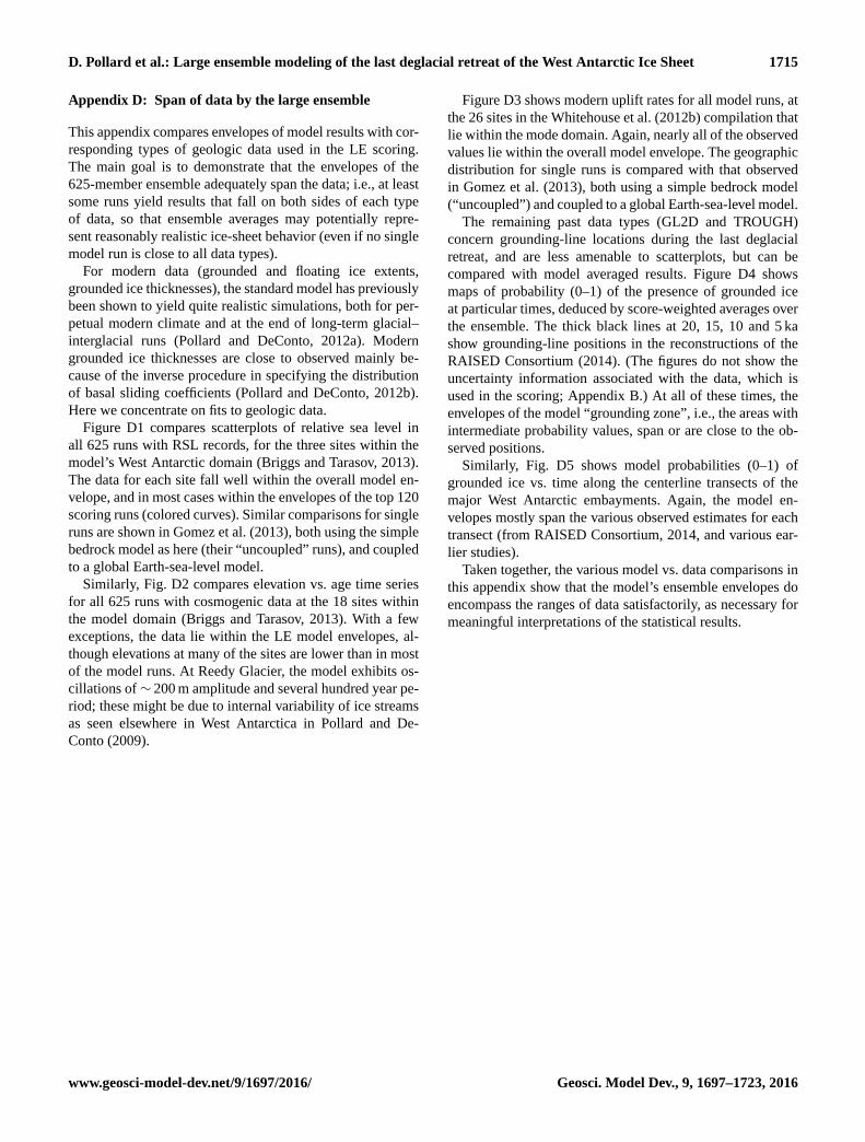
Figure D1 compares scatterplots of relative sea level in
all 625 runs with RSL records, for the three sites within the
model’s West Antarctic domain (Briggs and Tarasov, 2013).
The data for each site fall well within the overall model en-
velope, and in most cases within the envelopes of the top 120
scoring runs (colored curves). Similar comparisons for single
runs are shown in Gomez et al. (2013), both using the simple
bedrock model as here (their “uncoupled” runs), and coupled
to a global Earth-sea-level model.
Similarly, Fig. D2 compares elevation vs. age time series
for all 625 runs with cosmogenic data at the 18 sites within
the model domain (Briggs and Tarasov, 2013). With a few
exceptions, the data lie within the LE model envelopes, al-
though elevations at many of the sites are lower than in most
of the model runs. At Reedy Glacier, the model exhibits os-
cillations of∼ 200 m amplitude and several hundred year pe-
riod; these might be due to internal variability of ice streams
as seen elsewhere in West Antarctica in Pollard and De-
Conto (2009).
Figure D3 shows modern uplift rates for all model runs, at
the 26 sites in the Whitehouse et al. (2012b) compilation that
lie within the mode domain. Again, nearly all of the observed
values lie within the overall model envelope. The geographic
distribution for single runs is compared with that observed
in Gomez et al. (2013), both using a simple bedrock model
(“uncoupled”) and coupled to a global Earth-sea-level model.
The remaining past data types (GL2D and TROUGH)
concern grounding-line locations during the last deglacial
retreat, and are less amenable to scatterplots, but can be
compared with model averaged results. Figure D4 shows
maps of probability (0–1) of the presence of grounded ice
at particular times, deduced by score-weighted averages over
the ensemble. The thick black lines at 20, 15, 10 and 5 ka
show grounding-line positions in the reconstructions of the
RAISED Consortium (2014). (The figures do not show the
uncertainty information associated with the data, which is
used in the scoring; Appendix B.) At all of these times, the
envelopes of the model “grounding zone”, i.e., the areas with
intermediate probability values, span or are close to the ob-
served positions.
Similarly, Fig. D5 shows model probabilities (0–1) of
grounded ice vs. time along the centerline transects of the
major West Antarctic embayments. Again, the model en-
velopes mostly span the various observed estimates for each
transect (from RAISED Consortium, 2014, and various ear-
lier studies).
Taken together, the various model vs. data comparisons in
this appendix show that the model’s ensemble envelopes do
encompass the ranges of data satisfactorily, as necessary for
meaningful interpretations of the statistical results.
www.geosci-model-dev.net/9/1697/2016/ Geosci. Model Dev., 9, 1697–1723, 2016
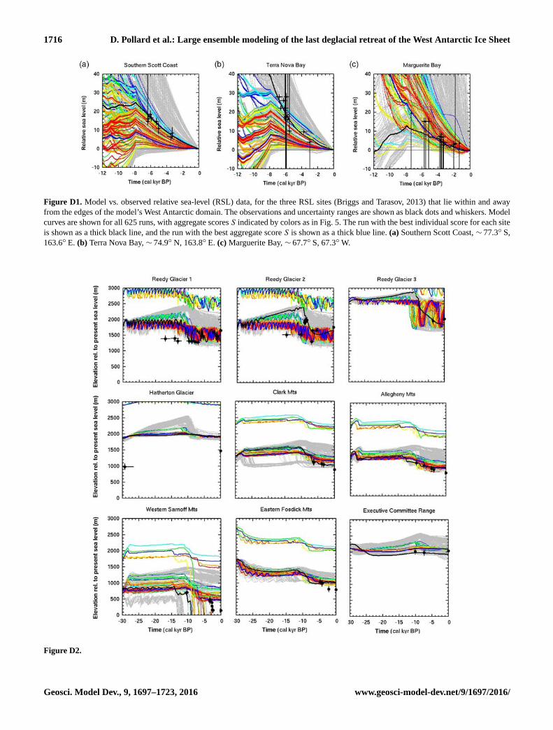
1716 D. Pollard et al.: Large ensemble modeling of the last deglacial retreat of the West Antarctic Ice Sheet
Figure D1. Model vs. observed relative sea-level (RSL) data, for the three RSL sites (Briggs and Tarasov, 2013) that lie within and away
from the edges of the model’s West Antarctic domain. The observations and uncertainty ranges are shown as black dots and whiskers. Model
curves are shown for all 625 runs, with aggregate scores S indicated by colors as in Fig. 5. The run with the best individual score for each site
is shown as a thick black line, and the run with the best aggregate score S is shown as a thick blue line. (a) Southern Scott Coast, ∼ 77.3◦ S,
163.6◦ E. (b) Terra Nova Bay, ∼ 74.9◦ N, 163.8◦ E. (c) Marguerite Bay, ∼ 67.7◦ S, 67.3◦W.
Figure D2.
Geosci. Model Dev., 9, 1697–1723, 2016 www.geosci-model-dev.net/9/1697/2016/
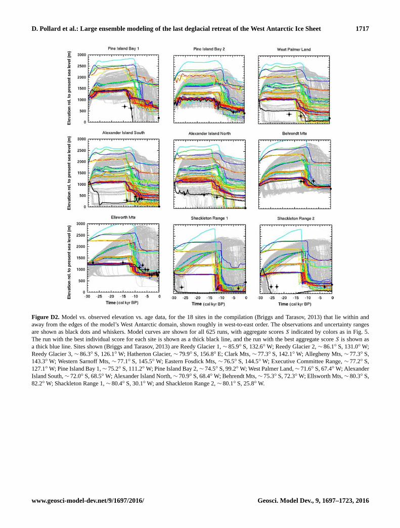
D. Pollard et al.: Large ensemble modeling of the last deglacial retreat of the West Antarctic Ice Sheet 1717
Figure D2. Model vs. observed elevation vs. age data, for the 18 sites in the compilation (Briggs and Tarasov, 2013) that lie within and
away from the edges of the model’s West Antarctic domain, shown roughly in west-to-east order. The observations and uncertainty ranges
are shown as black dots and whiskers. Model curves are shown for all 625 runs, with aggregate scores S indicated by colors as in Fig. 5.
The run with the best individual score for each site is shown as a thick black line, and the run with the best aggregate score S is shown as
a thick blue line. Sites shown (Briggs and Tarasov, 2013) are Reedy Glacier 1, ∼ 85.9◦ S, 132.6◦W; Reedy Glacier 2, ∼ 86.1◦ S, 131.0◦W;
Reedy Glacier 3, ∼ 86.3◦ S, 126.1◦W; Hatherton Glacier, ∼ 79.9◦ S, 156.8◦ E; Clark Mts, ∼ 77.3◦ S, 142.1◦W; Allegheny Mts, ∼ 77.3◦ S,
143.3◦W; Western Sarnoff Mts, ∼ 77.1◦ S, 145.5◦W; Eastern Fosdick Mts, ∼ 76.5◦ S, 144.5◦W; Executive Committee Range, ∼ 77.2◦ S,
127.1◦W; Pine Island Bay 1,∼ 75.2◦ S, 111.2◦W; Pine Island Bay 2,∼ 74.5◦ S, 99.2◦W; West Palmer Land,∼ 71.6◦ S, 67.4◦W; Alexander
Island South,∼ 72.0◦ S, 68.5◦W; Alexander Island North,∼ 70.9◦ S, 68.4◦W; Behrendt Mts,∼ 75.3◦ S, 72.3◦W; Ellsworth Mts,∼ 80.3◦ S,
82.2◦W; Shackleton Range 1, ∼ 80.4◦ S, 30.1◦W; and Shackleton Range 2, ∼ 80.1◦ S, 25.8◦W.
www.geosci-model-dev.net/9/1697/2016/ Geosci. Model Dev., 9, 1697–1723, 2016
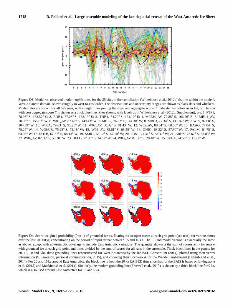
1718 D. Pollard et al.: Large ensemble modeling of the last deglacial retreat of the West Antarctic Ice Sheet
Figure D3. Model vs. observed modern uplift rates, for the 25 sites in the compilation (Whitehouse et al., 2012b) that lie within the model’s
West Antarctic domain, shown roughly in west-to-east order. The observations and uncertainty ranges are shown as black dots and whiskers.
Model rates are shown for all 625 runs, with straight lines joining the sites, and aggregate scores S indicated by colors as in Fig. 5. The run
with best aggregate score S is shown as a thick blue line. Sites shown, with labels as in Whitehouse et al. (2012b, Supplement), are: 1. FTP1,
78.93◦ S, 162.57◦ E; 2. ROB1, 77.03◦ S, 163.19◦ E; 3. TNB1, 74.70◦ S, 164.10◦ E; 4. MCM4_AV, 77.85◦ S, 166.76◦ E; 5. MBL1_AV,
78.03◦ S, 155.02◦W; 6. W01_AV, 87.42◦ S, 149.43◦W; 7. MBL2, 76.32◦ S, 144.30◦W; 8. MBL3, 77.34◦ S, 141.87◦W; 9. W09, 82.68◦ S,
104.39◦W; 10. W06A, 79.63◦ S, 91.28◦W; 11. W07_AV, 80.32◦ S, 81.43◦W; 12. W05_AV, 80.04◦ S, 80.56◦W; 13. HAAG, 77.04◦ S,
78.29◦W; 14. W08A/B, 75.28◦ S, 72.18◦W; 15. W02_AV, 85.61◦ S, 68.55◦W; 16. OHIG, 63.32◦ S, 57.90◦W; 17. PALM, 64.78◦ S,
64.05◦W; 18. ROTB, 67.57◦ S, 68.13◦W; 19. SMRT, 68.12◦ S, 67.10◦W; 20. FOS1, 71.31◦ S, 68.32◦W; 21. BREN, 72.67◦ S, 63.03◦W;
22. W04_AV, 82.86◦ S, 53.20◦W; 23. BELG, 77.86◦ S, 34.62◦W; 24. W03_AV, 81.58◦ S, 28.40◦W; 25. SVEA, 74.58◦ S, 11.22◦W.
Figure D4. Score-weighted probability (0 to 1) of grounded ice vs. floating ice or open ocean at each grid point (see text), for various times
over the last 20 000 yr, concentrating on the period of rapid retreat between 15 and 10 ka. The LE and model version is essentially the same
as above, except with all-Antarctic coverage to include East Antarctic variations. The quantity shown is the sum of scores S(n) for runs n
with grounded ice at each grid point and time, divided by the sum of scores for all runs in the ensemble. Thick black lines in the panels for
20, 15, 10 and 5 ka show grounding lines reconstructed for West Antarctica by the RAISED Consortium (2014), plotted using their vertex
information (S. Jamieson, personal communication, 2015), and choosing their Scenario A for the Weddell embayment (Hillenbrand et al.,
2014). For 20 and 15 ka around East Antarctica, the black line is from the 20 ka RAISED time slice that for the EAIS is based on Livingstone
et al. (2012) and Mackintosh et al. (2014). Similarly, the modern grounding line (Fretwell et al., 2013) is shown by a thick black line for 0 ka,
which is also used around East Antarctica for 10 and 5 ka.
Geosci. Model Dev., 9, 1697–1723, 2016 www.geosci-model-dev.net/9/1697/2016/
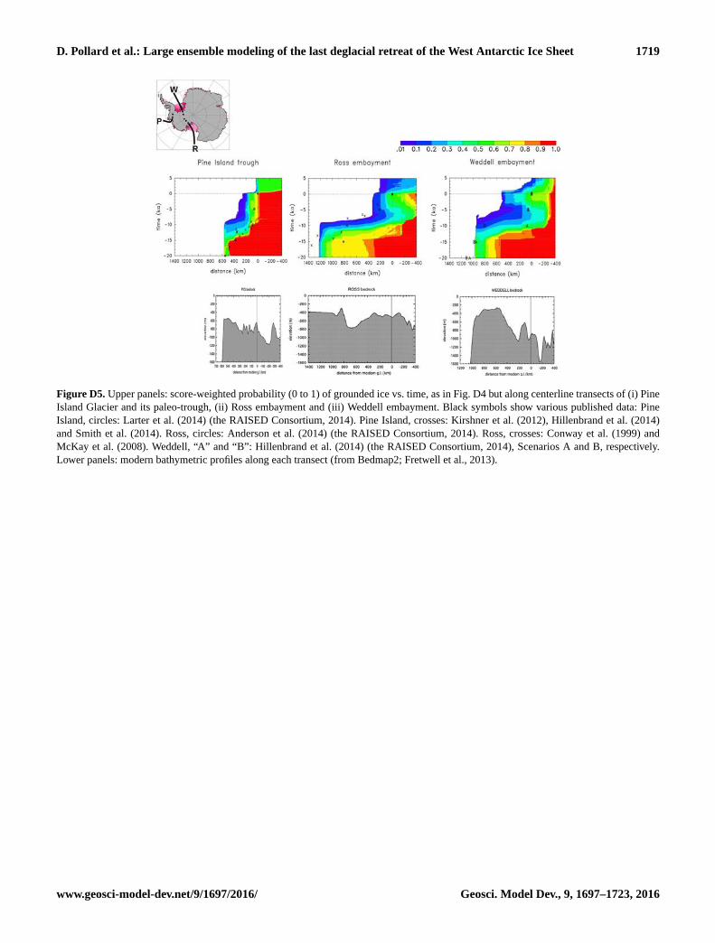
D. Pollard et al.: Large ensemble modeling of the last deglacial retreat of the West Antarctic Ice Sheet 1719
Figure D5. Upper panels: score-weighted probability (0 to 1) of grounded ice vs. time, as in Fig. D4 but along centerline transects of (i) Pine
Island Glacier and its paleo-trough, (ii) Ross embayment and (iii) Weddell embayment. Black symbols show various published data: Pine
Island, circles: Larter et al. (2014) (the RAISED Consortium, 2014). Pine Island, crosses: Kirshner et al. (2012), Hillenbrand et al. (2014)
and Smith et al. (2014). Ross, circles: Anderson et al. (2014) (the RAISED Consortium, 2014). Ross, crosses: Conway et al. (1999) and
McKay et al. (2008). Weddell, “A” and “B”: Hillenbrand et al. (2014) (the RAISED Consortium, 2014), Scenarios A and B, respectively.
Lower panels: modern bathymetric profiles along each transect (from Bedmap2; Fretwell et al., 2013).
www.geosci-model-dev.net/9/1697/2016/ Geosci. Model Dev., 9, 1697–1723, 2016
1720 D. Pollard et al.: Large ensemble modeling of the last deglacial retreat of the West Antarctic Ice Sheet
Acknowledgements. We thank Zhengyu Liu and his group
at U. Wisconsin for providing output of their coupled GCM
simulation (TraCE-21 ka; Liu et al., 2009; He et al., 2013;
www.cgd.ucar.edu/ccr/TraCE) used for ocean forcing over the last
20 000 yr. This work was supported in part by the following grants
from the National Science Foundation: NSF-DMS-1418090 and
the Network for Sustainable Climate Risk Management (SCRiM)
under NSF cooperative agreement GEO1240507 (DP, MH);
PLIOMAX OCE-1202632, OPP-1341394, and ANT-1443190
(DP); NSF Statistical Methods in the Atmospheric Sciences
Network 1106862, 1106974, and 1107046 (WC).
Edited by: P. Huybrechts
References
Anderson, J. B., Conway, H., Bart, P. J., Witus, A. E., Greenwood,
S. L., McKay, R. M., Hall, B. L., Ackert, R. P., Licht, K., Jakob-
sson M., and Stone, J. O.: Ross Sea paleo-ice sheet drainage
and deglacial history during and since the LGM, Quaternary Sci.
Res., 100, 31–54, 2014.
Applegate, P. J., Kirchner, N., Stone, E. J., Keller, K., and Greve, R.:
An assessment of key model parametric uncertainties in projec-
tions of Greenland Ice Sheet behavior, The Cryosphere, 6, 589–
606, doi:10.5194/tc-6-589-2012, 2012.
Bassett, S. E., Milne, G. A., Mitrovica, J. X., and Clark, P. U.: Ice
sheet and solid Earth influences on far-field sea-level histories,
Science, 309, 925–928, 2005.
Benn, D. I., Warren, C. R., and Mottram, R. H.: Calving processes
and the dynamics of calving glaciers, Earth-Sci. Rev., 82, 143–
179, 2007.
Briggs, R. D. and Tarasov, L.: How to evaluate model-derived
deglaciation chronologies: a case study using Antarctica, Qua-
ternary. Sci. Rev., 63, 109–127, 2013.
Briggs, R., Pollard, D., and Tarasov, L.: A glacial systems model
configured for large ensemble analysis of Antarctic deglacia-
tion, The Cryosphere, 7, 1949–1970, doi:10.5194/tc-7-1949-
2013, 2013.
Briggs, R. D., Pollard, D., and Tarasov, L.: A data-constrained large-
ensemble analysis of Antarctic evolution since the Eemian, Qua-
ternary Sci. Rev., 103, 91–115, 2014.
Chang, W., Applegate, P. J., Haran, M., and Keller, K.: Proba-
bilistic calibration of a Greenland Ice Sheet model using spa-
tially resolved synthetic observations: toward projections of ice
mass loss with uncertainties, Geosci. Model Dev., 7, 1933–1943,
doi:10.5194/gmd-7-1933-2014, 2014.
Chang, W., Haran, M., Applegate, P., and Pollard, D.: Calibrating
an ice sheet model using high-dimensional binary spatial data, J.
Am. Stat. Assoc., doi:10.1080/01621459.2015.1108199, online
first, 2015.
Chang, W., Haran, M., Applegate, P., and Pollard, D.: Improv-
ing ice sheet model calibration using paleoclimate and modern
data, available at: http://arxiv.org/abs/1510.01676, last access:
May 2016.
Chaput, J., Aster, R., Huerta, A., Sun, X., Lloyd, A., Wiens, D.,
Nyblade, A., Anandakishnan, S., Winberry, P., and Wilson, T.:
The crustal thickness of West Antarctica, J. Geophys. Res., 119,
1–18, doi:10.1002/2013JB010642, 2014.
Clark, P. U. and Tarasov, L.: Closing the sea level budget at the Last
Glacial Maximum, P. Natl. Acad. Sci., 111, 15861–15862, 2014.
Conway, H., Hall, B. L., Denton, G. H., Gades, A. M., and Wadding-
ton, E. D.: Past and future grounding-line retreat of the West
Antarctic Ice Sheet, Science, 286, 280–283, 1999.
Cornford, S. L., Martin, D. F., Graves, D. T., Ranken, F. R., Le
Brocq, A. M., Gladstone, R. M., Payne, A. J., Ng, E. G., and Lip-
scomb, W. H.: Adaptive mesh, finite volume modeling of marine
ice sheets, J. Comput. Phys., 232, 529–549, 2013.
DeConto, R. M. and Pollard, D.: Antarctica’s contribution to Last
Interglacial and future sea-level rise, Nature, 531, 591–597,
2016.
DeConto, R. M., Pollard, D., and Kowalewski, D.: Modeling
Antarctic ice sheet and climate variations during Marine Isotope
Stage 31, Global Planet. Change, 88–89, 45–52, 2012.
Deschamps, P., Durand, N., Bard, E., Hamelin, B., Camoin, G.,
Thomas, A. L., Henderson, G. M., Okuno, J., and Yokoyama,
Y.: Ice-sheet collapse and sea-level rise at the Bolling warming
14,600 years ago, Nature, 483, 559–564, 2012.
Docquier, D., Pollard, D., and Pattyn, F.: Thwaites Glacier
grounding-line retreat: Influence of width and buttressing param-
eterizations, J. Glaciol., 60, 305–313, 2014.
Durand, G., Gagliardini, O., Favier, L., Zwinger, T., and le Meur, E.:
Impact of bedrock description on modeling ice sheet dynamics,
Geophys. Res. Lett., 38, L20501, doi:10.1029/2011GL048892,
2011.
Dutrieux, P., De Rydt, J., Jenkins, A., Holland, P. R., Ha, H. K., Lee,
S. H., Steig, E. J., Ding, Q., Abrahamsen, E. P., and Schröder,
M.: Strong sensitivity of Pine Island ice-shelf melting to climatic
variability, Science, 373, 174–178, 2014.
Favier, L., Gagliardini, O., Durand, G., and Zwinger, T.: A three-
dimensional full Stokes model of the grounding line dynamics:
effect of a pinning point beneath the ice shelf, The Cryosphere,
6, 101–112, doi:10.5194/tc-6-101-2012, 2012.
Favier, L., Durand, G., Cornford, S. L., Gudmundsonn, G. H.,
Gagliardini, O., Gillet-Chaulet, F., Zwinger, T., Payne, A. J., and
Le Brocq, A. M.: Retreat of Pine Island Glacier controlled by
marine ice-sheet instability, Nature Clim. Change, 4, 117–121,
2014.
Fretwell, P., Pritchard, H. D., Vaughan, D. G., Bamber, J. L., Bar-
rand, N. E., Bell, R., Bianchi, C., Bingham, R. G., Blankenship,
D. D., Casassa, G., Catania, G., Callens, D., Conway, H., Cook,
A. J., Corr, H. F. J., Damaske, D., Damm, V., Ferraccioli, F., Fors-
berg, R., Fujita, S., Gim, Y., Gogineni, P., Griggs, J. A., Hind-
marsh, R. C. A., Holmlund, P., Holt, J. W., Jacobel, R. W., Jenk-
ins, A., Jokat, W., Jordan, T., King, E. C., Kohler, J., Krabill,
W., Riger-Kusk, M., Langley, K. A., Leitchenkov, G., Leuschen,
C., Luyendyk, B. P., Matsuoka, K., Mouginot, J., Nitsche, F. O.,
Nogi, Y., Nost, O. A., Popov, S. V., Rignot, E., Rippin, D. M.,
Rivera, A., Roberts, J., Ross, N., Siegert, M. J., Smith, A. M.,
Steinhage, D., Studinger, M., Sun, B., Tinto, B. K., Welch, B.
C., Wilson, D., Young, D. A., Xiangbin, C., and Zirizzotti, A.:
Bedmap2: improved ice bed, surface and thickness datasets for
Antarctica, The Cryosphere, 7, 375–393, doi:10.5194/tc-7-375-
2013, 2013.
Gohl, K., Uenzelmann-Neben, G., Larter, R. D., Hillenbrand, C.-D.,
Hochmuth, K., Kalberg, T., Weigelt, E., Davy, B., Kuhn, G., and
Nitsche, F. O.: Seismic stratigraphic record of the Amundsen Sea
Embayment shelf from pre-glacial to recent times: Evidence for
Geosci. Model Dev., 9, 1697–1723, 2016 www.geosci-model-dev.net/9/1697/2016/
D. Pollard et al.: Large ensemble modeling of the last deglacial retreat of the West Antarctic Ice Sheet 1721
a dynamic West Antarctic ice sheet, Marine Geol., 344, 115–131,
2013.
Gladstone, R. P., Lee, V., Rougier, J., Payne, A. J., Hellmer, H., Le-
Brocq, A. M., Shepherd, A., Edwards, T. L., Gregory, J., and
Cornford, S.: Calibrated prediction of Pine Island Glacier re-
treat during the 21st and 22nd centuries with a coupled flowline
model, Earth Planet. Sci. Lett., 333–334, 191–199, 2012.
Golledge, N. R., Fogwill, C. J., Mackintosh, A. N., and Buckley,
K. M.: Dynamics of the last glacial maximum Antarctic ice-
sheet and its response to ocean forcing, P. Natl. Acad. Sci., 109,
16052–16056, 2012.
Golledge, N. R., Levy, R. H., McKay, R. M., Fogwill, C. J., White,
D. A., Graham, A. G. C., Smith, J. A., Hillenbrand, C.-D., Licht,
K. J., Denton, G. H., Ackert Jr., R. P., Maas, S. M., and Hall,
B. L.: Glaciology and geological signature of the Last Glacial
Maximum Antarctic ice sheet, Quaternary Sci. Rev., 78, 225–
247, 2013.
Golledge, N. R., Menviel, L., Carter, L., Fogwill, C. J., England,
M. H., Cortese, G., and Levy, R. H.: Antarctic contribution to
meltwater pulse 1A from reduced Southern Ocean overturning,
Nature Comm., 5, 5107, doi:10.1038/ncomms6107, 2014.
Gomez, N., Pollard, D., and Mitrovica, J. X.: A 3-D coupled ice
sheet-sea level model applied to Antarctica through the last
40 kyr, Earth Planet. Sc. Lett., 384, 88–99, 2013.
Gomez, N., Pollard, D., and Holland, D.: Sea level feedback low-
ers projections of future Antarctic Ice Sheet mass loss, Nature
Commun., 6, 8798, doi:10.1038/ncomms9798, 2015.
He, F., Shakun, J. D., Clark, P. U., Carlson, A. E., Liu, Z., Otto-
Bliesner, B. L., and Kutzbach, J. E.: Northern Hemisphere forc-
ing of Southern Hemisphere climate during the last deglaciation,
Nature, 494, 81–85, 2013.
Hellmer, H., Kauker, F., Timmermann, R., Determann, J., and Rae,
J.: Twenty-first-century warming of a large Antarctic ice-shelf
cavity by a redirected coastal current, Nature, 485, 225–228,
2012.
Hillenbrand, C.-D., Bentley, M. J., Stolldorf, T., Hein, A. S., Kuhn,
G., Graham, A. C. G., Fogwill, C. J., Kristoffersen, Y., Smith, J.
A., Anderson, J. B., Larter, R. D., Melles, M., Hodgson, D. A.,
Mulvaney, R., and Sugden, D. E.: Reconstruction of changes in
the Weddell Sea sector of the Antarctic Ice Sheet since the Last
Glacial Maximum, Quaternary Sci. Rev., 100, 111–136, 2014.
Holland, P. R., Jenkins, A., and Holland, D. M.: The response of ice
shelf basal melting to variations in ocean temperature, J. Climate,
21, 2558–2572, 2008.
Holschuh, N., Pollard, D., Anandakrishnan, S., and Alley, R.: Eval-
uating Marie Byrd Land stability using an improved basal topog-
raphy, Earth Planet. Sc. Lett., 408, 362–369, 2014.
Huybrechts, P.: Sea-level changes at the LGM from ice-dynamic
reconstructions of the Greenland and Antarctic ice sheets during
the glacial cycles, Quaternary Sci. Rev., 21, 203–231, 2002.
Jakobsson, M., Anderson, J. B., Nitsche, F. O., Dowdeswell, J. A.,
Gyllencreutz, R., Kirchner, N., Mohammad, R., O’Regan, M.,
Alley, R. B., Anandakrishnan, S., Eriksson, B., Kirshner, A., Fer-
nandez, R., Stolldorf, T., Minzoni, R., and Majewski, W.: Geo-
logical record of ice shelf break-up and grounding line retreat,
Pine Island Bay, West Antarctica, Geology, 39, 691–694, 2011.
Joughin, I., Smith, B. E., and Medley, B.: Marine ice sheet col-
lapse potentially under way for the Thwaites Glacier basin, West
Antarctica, Science, 344, 735–738, 2014.
Kirshner, A. E., Anderson, J. B., Jakobsson, M., O’Regan, M., Ma-
jewski, W., and Nitsche, F. O.: Post-LGM deglaciation in Pine
Island Bay, West Antarctica, Quaternary Sci. Rev., 38, 11–26,
2012.
Konrad, H., Sasgen, S., Pollard, D., and Klemann, V.: Potential of
the solid-Earth response for limiting long-term West Antarctic
Ice Sheet retreat in a warming climate, Earth Planet. Sc. Lett.,
432, 254–264, 2015.
Larter, R. D., Anderson, J. B., Graham, A. G. C., Gohl, K., Hillen-
brand, C.-D., Jakobsson, M., Johnson, J. S., Kuhn, G., Nitsche,
F. O., Smith, J. A., Witus, A. E., Bentley, M. J., Dowdeswell, J.
A., Ehrmann, W., Klages, J. P., Lindow, J., Ó Cofaigh, C., and
Spiegel, C.: Reconstruction of changes in the Amundsen Sea and
Bellingshausen Sea sector of the West Antarctic Ice Sheet since
the Last Glacial Maximum, Quaternary Sci. Rev., 100, 55–86,
2014.
Le Brocq, A. M., Payne, A. J., and Vieli, A.: An improved
Antarctic dataset for high resolution numerical ice sheet
models (ALBMAP v1), Earth Syst. Sci. Data, 2, 247–260,
doi:10.5194/essd-2-247-2010, 2010.
Liu, Z., Otto-Bliesner, B. L., He, F., Brady, E. C., Tomas, R., Clark,
P. U., Carlson, A. E., Lynch-Stieglitz, J., Curry, W., Brook, E., Er-
ickson, D., Jacob, R., Kutzbach, J., and Cheng, J.: Transient sim-
ulation of last deglaciation with a new mechanism for Bølling-
Allerød warming, Science, 325, 310–314, 2009 (extended to
modern: www.cgd.ucar.edu/ccr/TraCE).
Livingstone, S. J., O Cofaigh, C., Stokes, C. R., Hillenbrand, C.-D.,
Vieli, A., and Jamieson, S. S. R.: Antarctic palaeo-ice streams,
Earth-Sci. Rev., 111, 90–128, 2012.
Mackintosh, A., Golledge, N., Domack, E., Dunbar, R., Leventer,
A., White, D., Pollard, D., DeConto, R., Fink, D., Zwartz, D.,
Gore, D., and Lavoie, C.: Retreat of the East Antarctic ice sheet
during the last glacial termination, Nat. Geosci., 4, 195–202,
2011.
Mackintosh, A. N., Verleyen, E., O’Brien, P. E., White, D. A., Jones,
R. S., McKay, R., Dunbar, R., Gore, D. B., Fink, D., Post, A. L.,
Miura, H., Leventer, A., Goodwin, I., Hodgson, D. A., Lilly, K.,
Crosta, X., Golledge, N. R., Wagner, B., Berg, S., van Ommen,
T., Zwartz, D., Roberts, S. J., Vyverman, W., and Masse, G.: Re-
treat history of the East Antarctic Ice Sheet since the Last Glacial
Maximum, Quaternary Sci. Rev., 100, 10–30, 2014.
Maris, M. N. A., van Wessem, J. M., van de Berg, W. J., de Boer,
B., and Oerlemans, J.: A model study of the effect of climate and
sea-level change on the evolution of the Antarctic Ice Sheet from
the Last Glacial Maximum to 2100, Clim. Dynam., 45, 837–851,
2015.
McKay, R. M., Dunbar, G. B., Naish, T. R., Barrett, P. J., Carter,
L., and Harper, M.: Retreat history of the Ross Ice Sheet (Shelf)
since the Last Glacial Maximum from deep-basin sediment cores
around Ross Island, Palaeogeogr. Palaeocl., 260, 245–261, 2008.
McNeall, D. J., Challenor, P. G., Gattiker, J. R., and Stone, E. J.: The
potential of an observational data set for calibration of a com-
putationally expensive computer model, Geosci. Model Dev., 6,
1715–1728, doi:10.5194/gmd-6-1715-2013, 2013.
Meinshausen, M., Smith, S. J., Calvin, K., Daniel, J. S., Kainuma,
M. L. T., Lamarque, J.-F., Matsumoto, K., Montzka, S. A., Raper,
S. C. B., Riahi, K., Thomson, A., Velders, G. J. M., and van Vu-
uren, D. P. P.: The RCP greenhouse gas concentrations and their
www.geosci-model-dev.net/9/1697/2016/ Geosci. Model Dev., 9, 1697–1723, 2016
1722 D. Pollard et al.: Large ensemble modeling of the last deglacial retreat of the West Antarctic Ice Sheet
extensions from 1765 to 2300, Climatic Change, 109, 213–241,
2011.
Mercer, J. H.: West Antarctic ice sheet and CO2 greenhouse effect:
a threat of disaster, Nature, 271, 321–325, 1978.
Morlighem, M., Rignot, E., Seroussi, H., Larour, E., Ben Dhia, H.,
and Aubry, D.: Spatial patterns of basal drag inferred using con-
trol methods from a full-Stokes and simpler models for Pine Is-
land Glacier, West Antarctica, Geophys. Res. Lett., 37, L14502,
doi:10.1029/2010GL043853, 2010.
Morlighem, M., Seroussi, H., Larour, E., and Rignot, E.: Inversion
of basal friction in Antarctica using exact and incomplete ad-
joints of a higher-order model, J. Geophys. Res.-Earth, 3, 1746–
1753, 2013.
Nick, F. M., van der Veen, C. J., Vieli, A., and Benn, D. I.: A phys-
ically based calving model applied to marine outlet glaciers and
implications for the glacier dynamics, J. Glaciol., 56, 781–794,
2010.
O Cofaigh, C., Davies, B. J., Livingstone, S. J., Smith, J. A., John-
son, J. S., Hocking, E. P., Hodgson, D. A., Anderson, J. B., Bent-
ley, M. J., Canals, M., Domack, E., Dowdeswell, J. A., Evans,
J., Glasser, N. F., Hillenbrand, C.-D., Larter, R. D., Roberts, S.
J., and Simms, A. R.: Reconstruction of Ice-Sheet Changes in
the Antarctic Peninsula Since the Last Glacial Maximum, Qua-
ternary Sci. Rev., 100, 87–110, 2014.
Parizek, B. R., Christianson, K., Anandakrishnan, S., Alley, R. B.,
Walker, R. T., Edwards, R. A., Wolfe, D. S., Bertini, G. T., Rine-
hart, S. K., Bindschadler, R. A., and Nowicki, S. M. J.: Dynamic
(in)stability of Thwaites Glacier, West Antarctica, J. Geophys.
Res.-Earth, 118, 638–655, 2013.
Pattyn, F., Perichon, L., Durand, G., Favier, L., Gagliardini, O.,
Hindmarsh, R. C. A., Zwinger, T., Albrecht, T., Cornford, S.,
Docquier, D., Furst, J. J., Goldberg, D., Gudmundsson, G. H.,
Humbert, A., Hutten, M., Huybrechts, P., Jouvet, G., Kleiner,
T., Larour, E., Martin, D., Morlighem, M., Payne, A. J., Pol-
lard, D., Ruckamp, M., Rybak, O., Seroussi, H., Thoma, M., and
Wilkens, N.: Grounding-line migration in plan-view marine ice-
sheet models: results of the ice2sea MISMIP3d intercomparison,
J. Glaciol., 59, 410–422, 2013.
Peltier, W. R.: Global glacial isostacy and the surface of the ice-age
Earth: The ICE-5G (VM2) model and GRACE, Annu. Rev. Earth
Planet. Sc., 32, 111–149, 2004.
Philippon, G., Ramstein, G., Charbit, S., Kageyama, M., Ritz, C.,
and Dumas, C.: Evolution of the Antarctic ice sheet throughout
the last deglaciation: A study with a new coupled climate – north
and south hemisphere ice sheet model, Earth Plan. Sc. Lett., 248,
750–758, 2006.
Pollard, D. and DeConto, R. M.: Modelling West Antarctic ice sheet
growth and collapse through the past five million years, Nature,
458, 329–332, 2009.
Pollard, D. and DeConto, R. M.: Description of a hybrid ice sheet-
shelf model, and application to Antarctica, Geosci. Model Dev.,
5, 1273–1295, doi:10.5194/gmd-5-1273-2012, 2012a.
Pollard, D. and DeConto, R. M.: A simple inverse method for the
distribution of basal sliding coefficients under ice sheets, applied
to Antarctica, The Cryosphere, 6, 953–971, doi:10.5194/tc-6-
953-2012, 2012b.
Pollard, D., DeConto, R. M., and Alley, R. B.: Potential Antarctic
Ice Sheet retreat driven by hydrofracturing and ice cliff failure,
Earth Plan. Sc. Lett., 412, 112–121, 2015.
Pollard, D., DeConto, R., Chang, W., Haran, M., and Applegate, P.:
Large ensemble modeling of the Antarctic Ice Sheet: Contribu-
tions to past and future sea-level rise, The Cryosphere Discuss.,
in preparation, 2016.
Pritchard, H. D., Ligtenberg, S. R. M., Fricker, H. A., Vaughan, D.
G., van den Broeke, M. R., and Padman, L.: Antarctic ice-sheet
loss driven by basal melting of ice shelves, Nature, 484, 502–505,
2012.
RAISED Consortium: A community-based geological reconstruc-
tion of Antarctic Ice Sheet deglaciation since the Last Glacial
Maximum, Quaternary Sci. Rev., 100, 1–9, 2014.
Rignot, E., Mouginot, J., Morlighem, M., Seroussi, H., and
Scheuchl, B: Widespread, rapid grounding line retreat of Pine
Island,Thwaites, Smith, and Kohler glaciers, West Antarctica,
from 1992 to 2011, Geophys. Res. Lett., 41, 3502–3509,
doi:10.1002/2014GL060140, 2014.
Ritz, C., Rommelaere, V., and Dumas, C.: Modeling the evolution of
Antarctic ice sheet over the last 420,000 years: Implications for
altitude changes in the Vostok region, J. Geophys. Res.-Atmos.,
106, 31943–31964, 2001.
Schoof, C.: Ice sheet grounding line dynamics: steady states, sta-
bility, and hysteresis, J. Geophys. Res.-Earth, 112, F03S28,
doi:10.1029/2006JF000664, 2007.
Shepherd, A., Ivins, E. K., Valentina, G. A., Barletta, R., Bentley,
M. J., Bettadpur, S., Briggs, K. H., Bromwich, D. H., Forsberg,
R., Galin, N., Horwath, M., Jacobs, S., Joughin, I., King, M. A.,
Lenaerts, J. T. M., Li, J., Ligtenberg, S. R. M., Luckman, A.,
Luthcke, S. B., McMillan, M., Meister, R., Milne, G., Moug-
inot, J., Muir, A., Nicolas, J.P., Paden, J., Payne, A. J., Pritchard,
H., Rignot, E., Rott, H., Sandberg L., Scambos, T. A., Scheuchl,
B., Schrama, E. J. O., Smith, B., Sundal, A. V., van Angelen, J.
H., van de Berg, W.J ., van den Broeke, M.R., Vaughan, D. G.,
Velicogna, I., Wahr, J., Whitehouse, P. L., Wingham, D. J., Yi,
D., Young, D., and Zwally, J.: A reconciled estimate of ice-sheet
mass balance, Science, 338, 1193–1198, 2012.
Smith, J. A., Hillenbrand, C.-D., Kuhn, G., Klages, J. P., Graham, A.
G. C., Larter, R. T., Ehrmann, W., Moreton, S. G., Wiers, S., and
Frederichs, T.: New constraints on the timing of West Antarc-
tic Ice Sheet retreat in the eastern Amundsen Sea since the last
Glacial Maximum, Global Planet. Change, 122, 224–237, 2014.
Stone, E. J., Lunt, D. J., Annan, J. D., and Hargreaves, J. C.: Quan-
tification of the Greenland ice sheet contribution to Last Inter-
glacial sea level rise, Clim. Past, 9, 621–639, doi:10.5194/cp-9-
621-2013, 2013.
Tarasov, L., Dyke, A. S., Neal, R. M., and Peltier, W. R.: A data-
calibrated distribution of deglacial chronologies for the North
American ice complex from glaciological modeling, Earth Plan.
Sc. Lett., 315–316, 30–40, 2012.
Urban, N. M. and Fricker, T. E.: A comparison of Latin hypercube
and grid ensemble designs for the multivariate emulation of an
Earth System model, Comput. Geosci., 36, 746–755, 2010.
Vaughan, D. G.: West Antarctic Ice Sheet collapse: the fall and rise
of a paradigm, Climatic Change, 91, 65–79, 2008.
Weber, M., Clark, P. U., Kuhn, G., Timmermann, A., Sprenk, D.,
Gladstone, D., Zhang, X., Lohmann, G., Menviel, L., Chikamoto,
M. O., Friedrich, T., and Ohlwein, C.: Millennial-scale variabil-
ity in Antarctic ice-sheet discharge during the last deglaciation,
Nature, 510, 134–138, 2014.
Geosci. Model Dev., 9, 1697–1723, 2016 www.geosci-model-dev.net/9/1697/2016/
D. Pollard et al.: Large ensemble modeling of the last deglacial retreat of the West Antarctic Ice Sheet 1723
Weertman, J.: Stability of the junction of an ice sheet and an ice
shelf, J. Glaciol., 13, 3–11, 1974.
Whitehouse, P. L., Bentley, M. J., and Le Brocq, A. M.: A deglacial
model for Antarctica: geological constraints and glaciological
modeling as a basis for a new model of Antarctic glacial isostatic
adjustment, Quaternary Sci. Res., 32, 1–24, 2012a.
Whitehouse, P. L., Bentley, M. J., Milne, G. A., King, M. A., and
Thomas, I. D.: A new glacial isostatic model for Antarctica: cal-
ibrated and tested using observations of relative sea-level change
and present-day uplifts, Geophys. J. Internat., 190, 1464–1482,
2012b.
www.geosci-model-dev.net/9/1697/2016/ Geosci. Model Dev., 9, 1697–1723, 2016