Embed Size (px)
Citation preview

RESEARCH REPORT July 2003 RR-03-19
Large Sample Tests for Comparing Regression Coefficients in Models With Normally Distributed Variables
Research & Development Division Princeton, NJ 08541
Alina A. von Davier


Large Sample Tests for Comparing Regression Coefficients in Models With Normally
Distributed Variables
Alina A. von Davier
Educational Testing Service, Princeton, NJ
July 2003

Research Reports provide preliminary and limited dissemination of ETS research prior to publication. They are available without charge from:
Research Publications Office Mail Stop 7-R Educational Testing Service Princeton, NJ 08541

Abstract
The analysis of regression coefficients is an important issue in different scientific areas, mostly
because conclusions about the relationship between variables, like causal interpretations, are
drawn based on these coefficients. This paper focuses on the description of the null hypothesis
of invariance of regression coefficients for multidimensional stochastic regressors. In this study,
it is assumed that the variables have a joint normal distribution with unknown expectation
and unknown positive definite covariance matrix. In this context, it is shown that the null
hypothesis contains special parameter points, called singular and stationary parameter points,
that influence the distribution of the commonly used test statistics under the null hypothesis.
Three large sample statistics—the Wald test, the likelihood ratio test, and the efficient score
test—are compared when testing this nonlinear null hypothesis. The results of a simulation
study are presented. The goal of the simulations is to check the distributions of the three
statistics for finite sample sizes and at a stationary point of the null hypothesis. Another
aim is to compare the empirical values of the three statistics to one another, for different
parameter constellations. It is shown that all three statistics present deviations from the
expected chi-squared distribution at this special parameter point. However, any of the three
statistical tests might be used for testing the hypothesis of the invariance of the regression
coefficients since they remain asymptotically conservative at the stationary points of the null
hypothesis.
Key words: Nonlinear hypothesis, Wald test, likelihood ratio test, efficient score test,
multivariate normal regressors
i

Acknowledgements
This paper is based on chapters 3, 4, and 5 of von Davier’s Ph.D. dissertation at
Otto-von-Guericke University, Magdeburg. The author wishes to thank Rolf Steyer and
Norbert Gaffke for their help and support during the dissertation process. The author also
thanks Shelby Haberman and Paul Holland for their feedback and suggestions on the previous
draft of this paper.
ii

1. Introduction
The analysis of regression coefficients is an important issue in different scientific
areas, mostly because conclusions about the relationship between variables are drawn based
on these coefficients. Many studies are carried out by investigating the regression coefficient
of the independent variable before and after adding other predictors into the linear model
(see Allison, 1995; Clogg, Petkova, & Haritou, 1995a, 1995b; Clogg, Petkova, & Shihadeh,
1992; Pratt & Schlaifer, 1988; Steyer, von Davier, Gabler, & Schuster, 1998). The main idea
underlying these studies is that if the change in the regression coefficients of the independent
variable before and after adding new variables to the regression is statistically significant, then
the simpler regression model (i.e., without the new regressors) offers a poorer or less complete
explanation of the independent variable of interest. Hence, different statistical procedures
have been investigated for testing whether the changes in the regression coefficients are
significant. The hypothesis of the invariance of the regression coefficients is introduced next.
Consider the regression of a real valued response variable Y on stochastic p- and
q-dimensional regressors X (the independent variable) and W (additional predictors),
respectively, where (Y, X ′, W ′)′ follow a (1 + p + q)-dimensional normal distribution, with
unknown expectation µ and unknown positive definite covariance matrix Σ. Then, as is
well-known, the conditional expectations E(Y |X) and E(Y |X,W ) are linear, that is,
E(Y |X) = α0 + α′X X, (1)
E(Y |X,W ) = β0 + β′X X + β′
W W , (2)
where α0, β0 ∈ IR, αX , βX ∈ IRp and βW ∈ IRq.
The hypothesis of invariance of the regression coefficients in regression models with
normally distributed variables reads:
H0 : αX = βX . (3)
Testing (3) based on the sample data represents the core of this paper. More exactly,
the goal of this paper is to compare three widely used large sample statistics (Wald test,
likelihood ratio test, and efficient score test) with respect to deviations from the expected
asymptotic χ2-distribution under the null hypothesis.
1

Previous research (von Davier, 2001; Gaffke, Steyer, & von Davier, 1999) concluded
that the null hypothesis of the invariance of the regression coefficients in regression models
with stochastic, normally distributed variables contains special parameter points, where the
Wald test does not asymptotically follow the χ2-distribution.
This paper focuses on two distinct aspects: (a) The description of the null hypothesis
of invariance of regression coefficients for stochastic variables. In this context, it is shown
that the null hypothesis contains special parameter points that influence the distribution of
the test statistics. It is important to note that this situation, (i.e., the existence of these
special parameter points in the null hypothesis), differs from model misspecification. (b) The
comparison of three large sample statistics—the Wald test, the likelihood ratio test, and the
efficient score test—when testing (3). It is shown that all three statistics have the same
deviations from the expected χ2-distribution at these points.
The rest of this paper is structured as follows. The next section sets up the notation
and formally introduces the null hypothesis; the definitions of the standard large sample
tests are recalled in Section 3. Section 4 shows how the statistical tests can be employed for
testing the null hypothesis on the basis of n identically independent distributed observations
from a multivariate normal distribution. Section 5 describes a simulation study where
cumulative distribution functions (cdfs) of the tests are compared over different sample sizes
and parameter constellations, and Section 6 contains additional discussion.
2. Hypothesis of Invariance of Regression Coefficients
The observations are modeled by (1 + p + q)-dimensional random variables
(Yi, X ′i,W
′i)′, i = 1, . . . , n, which are independent and identically normally distributed with
unknown expectation µ = (µY , µ′X , µ′
W )′ ∈ IR1+p+q and unknown positive definite covariance
matrix Σ. Then, the conditional expectations E(Yi |Xi) and E(Yi |Xi,W i), i = 1, . . . , n, are
linear:
E(Yi |Xi) = α0 + α′X Xi , (4)
E(Yi |Xi,W i) = β0 + β′X Xi + β′
W W i, (5)
where α0, β0 ∈ IR, αX , βX ∈ IRp, and βW ∈ IRq.
2

The unknown positive definite covariance matrix is
Σ =
ΣY Y Σ′
XY Σ′WY
ΣXY ΣXX Σ′WX
ΣWY ΣWX ΣWW
. (6)
The regression coefficients, αX , βX , and βW , in (4) and (5), are functions of Σ and µ, and
can be obtained from
αX = Σ−1XX ΣXY , (7) βX
βW
=
ΣXX Σ′WX
ΣWX ΣWW
−1 ΣXY
ΣWY
(8)
(cf. Rao, 1973, p. 522 (8a.2.11)). Denote
C =(ΣWW −ΣWXΣ−1
XXΣ′WX
)−1. (9)
It can be shown that
βX = (Σ−1XX + Σ−1
XXΣ′WXCΣWXΣ−1
XX)ΣXY
−Σ−1XXΣ′
WXCΣWY , (10)
βW = C(ΣWY −ΣWXΣ−1XXΣXY ) , (11)
with C from (9) (see also Gaffke et al., 1999).
From (7), (10), and (11) it follows that αX − βX = Σ−1XXΣ′
WXβW , and thus the null
hypothesis (3) equivalently reads as
H0 : Σ−1XX Σ′
WX βW = 0 . (12)
From (12), it is obvious that Σ−1XX does not influence the testing of the null hypothesis
(3). However, given that the focus is on the invariance of regression coefficients, that is, on
testing (3), and that (12) is its product equivalent form, I decided to keep Σ−1XX . Moreover,
since one might be interested in the confidence interval around the difference of interest,
αX − βX = Σ−1XX Σ′
WX βW , one would like to keep Σ−1XX for consistency.
The nonlinear restriction function describing H0, denoted R in this paper,
depends on the parameter vector θ, where θ consists of the expectation µ and of the
3
entries within and below the diagonal of the covariance matrix Σ. The dimension of θ is
m = (1 + p + q)(4 + p + q)/2 and that of R(θ) is p, that is, R : IRm −→ IRp, with
R(θ) = Σ−1XXΣ′
WXβW = Σ−1XXΣ′
WXC(ΣWY −ΣWXΣ−1
XXΣXY
), (13)
with βW from (11).
The standard large sample statistics usually employed for testing nonlinear
hypotheses require a full row rank of the Jacobian of the restriction function, JR(θ), in
order to be applicable (cf. Godfrey, 1988, pp. 5–17; Rao, 1973, pp. 415–419; White, 1982,
Theorem 3.4). The entries of JR(θ) are the partial derivatives of R with respect to the
components of θ. Gaffke et al. (1999) and von Davier (2001) showed that the Jacobian does
not always have a full row rank under the null hypothesis and moreover, that it might vanish
under special circumstances. The rank of the Jacobian is described by the following lemma,
which is proved in Gaffke et al. (1999) and in von Davier (2001).
Lemma 2.1 Let θ and βW be defined as above. Consider the Jacobian, JR(θ), of R(θ) =
Σ−1XXΣ′
WXβW .
(a) If βW 6= 0, then rank(JR(θ))= p ;
(b) If βW = 0, then rank(JR(θ)) = rank(ΣWX) .
Thus, by the lemma, there are parameter values in the null hypothesis with a rank
deficient Jacobian, namely those with βW = 0 and rank(ΣWX) < p (which will be called
singular parameter points of H0). A particular case is βW = 0 and ΣWX = 0, where the
Jacobian vanishes (which will be called stationary parameter points of H0).
We also observe that the null hypothesis may have special parameter points (singular
parameter points) when βW = 0 and rank(ΣWX) < q < p.
As shown in the next section, the singular and stationary points of the null hypothesis
involve the consideration of an additional analysis of the (investigated) statistical tests,
because the tests do not asymptotically follow the χ2-distribution at these points.
3. Large Sample Tests
First, the definitions of the Wald test, the likelihood ratio test, and the efficient score
test will be recalled.
4

Let the statistical model (for each n ∈ IN) be:
(Ω(n), A(n),
P
(n)θ : θ ∈ Θ
), Θ ⊂ IRm (open set). (14)
Assumption 3.1 Assume that the regularity conditions (on the log-likelihood function of the
sample, ln) required for maximum likelihood estimation are fulfilled.(See, for example, the
regularity conditions given by Godfrey, 1988, pp. 6–7.)
Hence, the maximum likelihood estimator of θ, θn, (where n denotes the sample size
increasing to infinity) is an asymptotically normal estimator. That is,
√n (θn − θ) D−→ N (0,V(θ)) (convergence in distribution) (15)
for all θ ∈ Θ, where N (0,V(θ)) denotes the multivariate normal distribution with expectation
zero and covariance matrix V(θ), with V(θ), positive definite for all θ ∈ Θ. Usually V(θ) will
be the inverse of the Fisher information matrix.
Assumption 3.2 Assume that V( · ) is continuous on Θ.
The so-called standard large sample tests—the Wald test (Wn), the likelihood ratio test
(LRn), and the efficient score test (ESn) (or, equivalently, the Lagrange multiplier LMn)—are
usually employed for testing a null hypothesis on a m-dimensional parameter θ from a
statistical model as in (14),
H0 : R(θ) = 0, (16)
where R = (R1, . . . , Rr)′ is a given function on the parameter space Θ ⊂ IRm with values in
IRr.
Assumption 3.3 Assume that the dimension of the restriction function is smaller than the
dimension of the parameter θ, that is, r ≤ m.
Assumption 3.4 Assume that R is continuously differentiable on Θ.
Let J(θ) denote the Jacobian of R at θ, which is the r×m matrix with entries (∂Rk/∂θj) (θ),
1 ≤ k ≤ r, 1 ≤ j ≤ m.
5

Theorem 3.1 (Wald test) Let Assumptions 1, 2, 3, and 4 be valid and θn be the unrestricted
ML estimator of θ. Then, for any θ from the null hypothesis from (3) such that J(θ) has a
full rank r, the Wald statistic
Wn = n R(θn)′(J(θn)V(θn)J(θn)′ )−1R(θn) (17)
is asymptotically χ2-distributed with r degrees of freedom, that is,
WnD−→ χ2
r , (18)
(cf. Godfrey, 1988, pp. 5–17; Rao, 1973, pp. 415–419; White, 1982, Theorem 3.4).
Theorem 3.2 (Likelihood ratio test) Let Assumptions 1, 2, 3, and 4 be valid; θn be the
unrestricted; and θn be the restricted maximum likelihood estimators of θ. Then the likelihood
ratio statistic is
LRn = 2( ln(θn)− ln(θn) ), (19)
where ln is the log-likelihood of the sample. For any θ from the null hypothesis such that J(θ)
has a full rank r, LRn is asymptotically χ2-distributed with r degrees of freedom, that is,
LRnD−→ χ2
r , (20)
(cf. Rao, 1973, pp. 415–419).
The score vector is defined as
Dn(θ) =∂ln(θ)
∂θ, (21)
where ln is the log-likelihood of the sample (see, for example, Godfrey, 1988; Rao, 1973;
White, 1982).
Theorem 3.3 (Efficient Score Test) Let Assumptions 1, 2, 3, and 4 be valid; θn be the
restricted ML estimator of θ; and Dn be the score vector. Then, for any θ from the null
hypothesis such that J(θ) has a full rank r, the efficient score statistic,
ESn = Dn(θn)′V(θn)Dn(θn), (22)
is asymptotically χ2-distributed with r degrees of freedom, that is,
ESnD−→ χ2
r , (23)
(cf. Rao, 1973, pp. 415–419;).
6

Significantly large values of each of the tests lead to the rejection of the null
hypothesis.
In linear regression models with identically independently normally distributed errors
and linear restrictions on the parameters where the error covariance matrix is unknown, the
following numerical inequality exists among the sample values of the Wald test, the likelihood
ratio test, and the efficient score test (Breusch, 1979; Godfrey, 1988):
Wn ≥ LRn ≥ ESn. (24)
In addition, Breusch (1979, p. 206) showed that
LRn ≥ ESn, (25)
if the restrictions are nonlinear.
When used for testing the invariance of regression coefficients, the three statistics are
expected to satisfy (25) and not (24), because the restriction function that describes the null
hypothesis from (3) is nonlinear.
Gaffke et al. (1999, Theorem 2.1) showed that the asymptotic distribution of the
Wald statistic at a stationary point of the null hypothesis, that is, at a point θ0 ∈ Θ such that
R(θ0) = 0 and J(θ0) = 0, differs from the standard result given in Theorem 3.1. Gaffke et al.
(1999, Lemma 3.4) proved that, for p = 1 and at a stationary point of the null hypothesis,
the Wald statistic remains asymptotically conservative. von Davier (2001) numerically
showed that the Wald statistic also remains asymptotically conservative at the singular and
stationary points for the case of multidimensional regressors. Then, it is naturally to ask if
the asymptotic null distribution of the Wald statistic at singular parameter points differs from
standard χ2-distribution, what would happened to the other large sample statistics at the
same points. Would they do any better than the Wald test? Also, as seen in (19) and in (22),
the formulas for the likelihood ratio test and the efficient score test do not explicitly depend
on the Jacobian matrix, although the full row rank assumption on the Jacobian is necessary
for the tests in order to be χ2r . For this reason it does make sense to check their distribution
at the singular points of the null hypothesis.
7
4. Testing Invariance of Regression Coefficients
In this section, the statistics described before are applied to test the null hypothesis
given in (3). The procedure for testing the null hypothesis is carried out in three steps:
(a) the restriction function R and the parameter θ are identified; (b) it is shown how to
obtain the unrestricted and the restricted maximum likelihood estimators, which fulfill the
corresponding assumptions; and (c) the empirical values of the Wald test, likelihood ratio
test, and efficient score test are computed from (17), (19), and (22), respectively.
In order to apply the tests to (3), let the function R be defined as in (13) and the
parameter θ consist of the expectation µ and of the entries within and below the diagonal of
the covariance matrix Σ, as shown in Section 2.
Computing the unrestricted ML estimator. The maximum likelihood (ML) estimator
of θ is given by Y , X, W (the sample means), and by the entries within and below the
diagonal of the sample covariance matrix
Σ =1n
n∑i=1
Yi − Y
Xi −X
W i −W
(
Yi − Y , X ′i −X
′, W ′
i −W′
). (26)
Note that θn satisfies (15)—it follows from the Central Limit Theorem. The asymptotic
covariance matrix of√
n (θn − θ) under θ from (15) is given by
V(θ) =
Σ 0
0 V1(θ)
(27)
with Σ from (6). V1(θ) is the asymptotic covariance matrix of the 12d(d + 1) × 1-vector
formed from the nonduplicated elements of (from the the lower half and the diagonal of)√
n(Σ−Σ), with d = 1 + p + q. In order to describe V1(θ), let Σ = (Σij)i,j=1,...,d, and index
the rows and columns of V1(θ) by pairs (i, j) and (`,m), respectively, where 1 ≤ i ≤ j ≤ d
and 1 ≤ ` ≤ m ≤ d. Browne (1982, pp. 81-82) showed that, when the variables have a joint
multivariate normal distribution—as in this study—the entries of V1(θ),
V1,(i,j)(`,m)(θ) = nCov(Σij , Σ`m
), (28)
where n is the sample size (see also Kendall & Stuart, 1969, p. 321), might be expressed as
V1,(i,j)(`,m)(θ) = Σi`Σjm + ΣimΣj`. (29)
8

Recall that the covariance matrix from (6), Σ, is assumed to be positive definite and,
therefore, also the asymptotic covariance matrix, V1(θ), defined in (28) is positive definite
(see also Rao, 1973, p. 107). Hence, from (27)–(29), it can be seen that V(θ) is positive
definite and it continuously depends on θ (see also Browne, 1982, p. 81–83).
Computing the restricted ML estimator. If ( Yi, X ′i, W ′
i )′, i = 1, . . . , n are
independent and identically normally distributed, then the logarithm of the density function
of the normal distribution can be computed.
Let U i = (Yi, X ′i, W ′
i )′, i = 1, . . . , n and d = 1 + p + q. Denote θ = (µ,Σ∗), where
Σ∗ contains the entries within and below the diagonal of the covariance matrix Σ. Then
p(U i,θ) =(
12π
)d/2 (1
detΣ
)1/2
exp−1
2(U i − µ)′Σ−1(U i − µ)
.
Thus,
ln(θ) =n∑1
log p(U i, θ)
= k − n
2log(det(Σ))− 1
2
n∑1
(U i − µ)′Σ−1(U i − µ),
where k is a constant.
Although θ consists of (µ,Σ∗), the restriction function depends only on Σ∗. The
constrained maximization problem is maxθ∈Θ ln(θ), under the restriction R(Σ∗) = 0.
Hence,
µ = µ = U .
ln(θ) = ln(U ,Σ∗) (30)
=−n
2log(detΣ)− 1
2
n∑1
(U i − U)′Σ−1(U i − U) (31)
= −n
2[log(detΣ) + tr(Σ−1Σ)], (32)
where, as in (26), Σ = 1n
∑n1 (U i − U)′(U i − U). If the Lagrangean is introduced, then
Λ(θ, λ) = ln(θ) + λ′R(θ),
where λ is a vector of Lagrangean multipliers. The elements of θn then satisfy the equations
Dn(θ) + JR(θ)′λ = 0, (33)
R(θ) = 0,
9
where λ is the vector of estimated multipliers and Dn is the score vector from (21) (see, for
example, Aitchison & Silvey, 1958).
From (33) we observe that the Lagrangean multipliers depend on the Jacobian matrix
of the restriction function. Hence, through (33), both the efficient score and the likelihood
ratio test depend on the Jacobian of the restriction function.
In this study, θn is not derived following this analytical method (or the numerical
approach described in Aitchison & Silvey, 1958). For computational purposes, the restricted
maximum likelihood is obtained slightly differently in a way that is described in the next
section.
Next, θn is used to compute the empirical values of the Wald test. Then, θn is used
to compute the likelihood ratio statistic, LRn, as described in Theorem 3.2. The score test
vector at θn, that is Dn(θn), and the asymptotic covariance matrix at θn, V(θn), have to be
calculated in order to compute the efficient score test, ESn.
5. Simulation Studies
The goal of the simulations is to check the distribution of the statistical tests for
finite sample sizes and for stationary parameter points of the null hypothesis. Another aim is
to compare the likelihood ratio and the efficient score statistics to the Wald test under H0.
This is achieved by computing the empirical values of the three statistics under (3) for three
different sets of parameter values. The three cdfs are plotted for each of the three sets of
parameters.
The data generation was done by Monte Carlo simulation of nΣ from a central
(d = 1+ p + q)-dimensional Wishart distribution with n− 1 degrees of freedom and parameter
Σ, where Σ is the sample covariance matrix entering into the Wald statistic (see von Davier,
2001, for a detailed description of the algorithm).
The simulations were performed assuming a linear regression model with normally
distributed variables with one-dimensional regressors (p = q = 1). The model is
Yi = β0 + βXXi + βW Wi + νi, (34)
where Y is a real valued response variable, X and W are one-dimensional regressors, β0, βX ,
βW ∈ IR, and i = 1, . . . , n, where n is the sample size.
10
The dimensions p = q = 1 of X and W , the (population) covariance matrix ΣWX ,
and the values of βX and βW were given as an input. The variances ΣXX and ΣWW
are fixed to 100. The covariances ΣXY and ΣWY were computed from (34) by assuming
Cov(νi, Xi) = Cov(νi, Wi) = 0; the error variance σ2ν was calculated so that the variance ΣY Y
was 100.
Thus, a 3 × 3-matrix Σ was obtained. Further, nΣ was simulated from a central
Wishart distribution, W(3)(n− 1,Σ).
The (3) × (3)-matrix Σ is distributed as the maximum likelihood estimates of Σ,
based on samples of n observations from a (3 = 1 + p + q)-variate normal distribution with
population covariance matrix Σ and an unknown expectation µ (Browne, 1982, p. 276–277;
Rao, 1973, pp. 533-540).
Three cases (three sets of parameter values), representing the relevant cases described
in Lemma 2.1, were investigated: a nonsingular point of the null hypothesis such that
ΣWX = 0 and βW 6= 0, a nonsingular point such that ΣWX 6= 0 and βW = 0, and a stationary
point of the null hypothesis, that is, ΣWX = 0 and βW = 0. Note that if p = 1, then any
singular point is a stationary point of the null hypothesis. Note also that if p = 1, then a case
where ΣWX 6= 0 and βW = 0 is still a nonsingular case, because the rank of the Jacobian
is still p = 1. The cases are presented in Table 1. For each case, 1,000 simulations were
performed. The investigated sample sizes were n = 50, 100, 200, 500, 1, 000, and 10, 000.
Note on the likelihood ratio test and the efficient score test. As mentioned earlier
in this study, θn is not derived following the analytical method presented in Section 4,
Table 1.
Cases Where the Null Hypothesis of the Regression of Y on X With Respect to W Holds
Case 1 Case 2 Case 3
ΣWX βW ΣWX βW ΣWX βW
0 0.3 30 0 0 0
Note. If the covariances are divided by 100, the results can be interpreted as correlations. p = 1 and
q = 1, βX = 0.2, ΣXX = ΣWW = ΣY Y = 100.
11
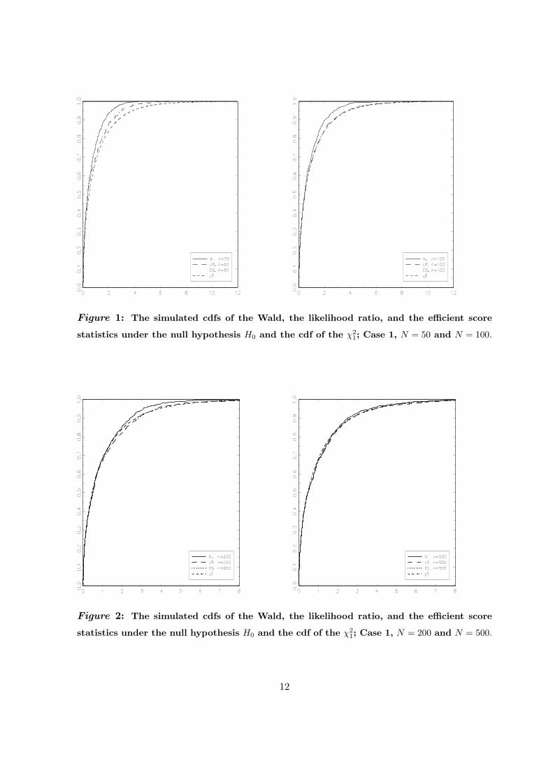
Figure 1: The simulated cdfs of the Wald, the likelihood ratio, and the efficient score
statistics under the null hypothesis H0 and the cdf of the χ21; Case 1, N = 50 and N = 100.
Figure 2: The simulated cdfs of the Wald, the likelihood ratio, and the efficient score
statistics under the null hypothesis H0 and the cdf of the χ21; Case 1, N = 200 and N = 500.
12

Figure 3: The simulated cdfs of the Wald, the likelihood ratio, and the efficient score
statistics under the null hypothesis H0 and the cdf of the χ21; Case 1, N = 1, 000 and
N = 10, 000.
because the data generation was done by Monte Carlo simulation of nΣ from a central
(1 + p + q = 3)-dimensional Wishart distribution with n− 1 degrees of freedom and parameter
Σ. The logarithm of the density function of the Wishart distribution can be computed (see
Rao, 1973, pp. 597–598, Complements 11.4 and 11.5) instead of the logarithm of the density
function of the normal distribution, ln, from (32). (Note that the restriction function depends
only on the components of Σ.) The obtained likelihood of the sample, denoted lwn , was
used to compute the θn, by employing the Constrained Maximum Likelihood–GAUSS 3.0
Application (1995). This software package uses Sequential Quadratic Programming (SQP)
method (see also Thisted, 1988). In this method, the parameters are updated in a series of
iterations beginning with provided starting values. SQP method requires the calculation of
the Jacobian and the Hessian of the lwn , as well as the Jacobian of the restriction function.
It also makes use of the vector of the Lagrangean coefficients of the equality constraints (see
Constrained Maximum Likelihood–GAUSS 3.0 Application, 1995, pp. 8–17).
The score test vector at θn, Dn(θn), and the asymptotic covariance matrix at θn,
V(θn), were also calculated in order to compute the efficient score test.
13
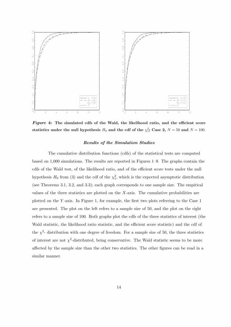
Figure 4: The simulated cdfs of the Wald, the likelihood ratio, and the efficient score
statistics under the null hypothesis H0 and the cdf of the χ21; Case 2, N = 50 and N = 100.
Results of the Simulation Studies
The cumulative distribution functions (cdfs) of the statistical tests are computed
based on 1,000 simulations. The results are reported in Figures 1–9. The graphs contain the
cdfs of the Wald test, of the likelihood ratio, and of the efficient score tests under the null
hypothesis H0 from (3) and the cdf of the χ21, which is the expected asymptotic distribution
(see Theorems 3.1, 3.2, and 3.3); each graph corresponds to one sample size. The empirical
values of the three statistics are plotted on the X-axis. The cumulative probabilities are
plotted on the Y -axis. In Figure 1, for example, the first two plots referring to the Case 1
are presented. The plot on the left refers to a sample size of 50, and the plot on the right
refers to a sample size of 100. Both graphs plot the cdfs of the three statistics of interest (the
Wald statistic, the likelihood ratio statistic, and the efficient score statistic) and the cdf of
the χ2- distribution with one degree of freedom. For a sample size of 50, the three statistics
of interest are not χ2-distributed, being conservative. The Wald statistic seems to be more
affected by the sample size than the other two statistics. The other figures can be read in a
similar manner.
14
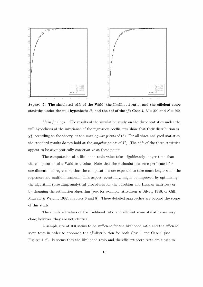
Figure 5: The simulated cdfs of the Wald, the likelihood ratio, and the efficient score
statistics under the null hypothesis H0 and the cdf of the χ21; Case 2, N = 200 and N = 500.
Main findings. The results of the simulation study on the three statistics under the
null hypothesis of the invariance of the regression coefficients show that their distribution is
χ21, according to the theory, at the nonsingular points of (3). For all three analyzed statistics,
the standard results do not hold at the singular points of H0. The cdfs of the three statistics
appear to be asymptotically conservative at these points.
The computation of a likelihood ratio value takes significantly longer time than
the computation of a Wald test value. Note that these simulations were performed for
one-dimensional regressors, thus the computations are expected to take much longer when the
regressors are multidimensional. This aspect, eventually, might be improved by optimizing
the algorithm (providing analytical procedures for the Jacobian and Hessian matrices) or
by changing the estimation algorithm (see, for example, Aitchison & Silvey, 1958, or Gill,
Murray, & Wright, 1982, chapters 6 and 8). These detailed approaches are beyond the scope
of this study.
The simulated values of the likelihood ratio and efficient score statistics are very
close; however, they are not identical.
A sample size of 100 seems to be sufficient for the likelihood ratio and the efficient
score tests in order to approach the χ21-distribution for both Case 1 and Case 2 (see
Figures 1–6). It seems that the likelihood ratio and the efficient score tests are closer to
15

Figure 6: The simulated cdfs of the Wald, the likelihood ratio, and the efficient score
statistics under the null hypothesis H0 and the cdf of the χ21; Case 2, N = 1, 000 and
N = 10, 000.
the χ21-distribution for small and medium sample sizes, than the Wald test. If the sample
size increases, then the three statistics have very close empirical values and approximate the
χ21-distribution for both Case 1 and Case 2.
For a stationary point of the null hypothesis, the results of the simulations indicate
that none of the three statistics are χ21-distributed for all sample sizes (see Figures 7–9).
However, the three statistics remain asymptotically conservative.
The numerical inequality for nonlinear restrictions given in (25) holds for all analyzed
cases and finite sample sizes. The Wald test values appear to be smaller than those of the
efficient score test and, therefore, for the model from Table 1, the numerical relationship
between the three tests is
LRn ≥ ESn ≥ Wn
for small and medium sample sizes. However, the analysis of additional models leads to the
observation that the empirical values of the Wald test increase when the value of the nonzero
term of the product ΣWXβW increases. For example, if ΣWX = 0 and βW = 0.7, then the
numerical inequality for small and medium sample sizes between the three tests is
LRn ≥ Wn ≥ ESn.
16

Figure 7: The simulated cdfs of the Wald, the likelihood ratio, and the efficient score
statistics under the null hypothesis H0 and the cdf of the χ21; Case 3, N = 50 and N = 100.
Figure 8: The simulated cdfs of the Wald, the likelihood ratio, and the efficient score
statistics under the null hypothesis H0 and the cdf of the χ21; Case 3, N = 200 and N = 500.
17

Figure 9: The simulated cdfs of the Wald, the likelihood ratio, and the efficient score
statistics under the null hypothesis H0 and the cdf of the χ21; Case 3, N = 1, 000 and
N = 10, 000.
The results on the three statistics for this example are given in von Davier (2001,
Appendix C). It seems that the Wald test is more sensitive than the other tests to a variation
in the size of the parameter values. Recall that the Wald test formula is the only one of the
three tests that explicitly depends on the Jacobian of the restriction function.
6. Discussion and Conclusions
The distribution of the Wald statistic was closely analyzed in von Davier (2001)
under the null hypothesis for multidimensional regressors at nonsingular, singular, and
stationary parameter values, as well as for different sample sizes. It was theoretically proved
that for a one-dimensional X, the Wald test is asymptotically conservative at stationary
parameter points (see also Gaffke et al., 1999). From the simulation study presented in von
Davier (2001), it might be conjectured that its conservative behavior at these points also
holds for the multidimensional regressors X and W .
The numerical results on the likelihood ratio test and the efficient score test presented
here indicate that both behave (asymptotically) similarly to the Wald test. That is, they
follow a χ21-distribution at the nonsingular points of H0 and remain conservative at the
stationary points. The likelihood ratio and the efficient score tests seem to perform better
18

than the Wald test when testing the null hypothesis for small and medium sample sizes (50,
100, and 200) for the cases from Table 1. For this reason, it is desirable to investigate the
likelihood ratio test and the efficient score test in more detail. However, for other parameter
values, the Wald test is as good as the other two standard large sample tests (see von Davier,
2001, Appendix C).
An additional large sample test, which was proposed by Clogg et al. (1995b) (the
CPH test), was also investigated numerically by von Davier (2001). The results obtained for
the CPH test were compared to the Wald test, and the same deviations from the expected
distribution were found. (The CPH test is supposed to be asymptotically normally distributed
under H0 and for one-dimensional predictors. Therefore, von Davier (2001) compares the
squared values of the CPH test with the values of the Wald test.) The analysis presented in
von Davier (2001) concluded that the CPH test needs further numerical studies in order to see
how the statistic is distributed at the singular points of H0 for multidimensional regressors.
From the simulation study presented in this paper, it might be concluded that any
of the three well-known statistics that were analyzed here might be used for testing (3).
They all present deviations from the standard results at stationary parameter points of the
null hypothesis, being asymptotically conservative at these points. Taking into account that
singular and stationary parameter points occur in the null hypothesis, the power of the test is
not decreased.
19

References
Aitchison, J. & Silvey, S. D. (1958). Maximum likelihood estimation of parameters subject
to restraints. Annals of Mathematical Statistics, 29, 813-828.
Allison, P. D. (1995). The impact of random predictors on comparison of coefficients
between models: Comment on Clogg, Petkova, and Haritou. American Journal of
Sociology, 100, 1294–1305.
Breusch, T. S. (1979). Conflict among criteria for testing hypotheses: Extensions and
comments. Econometrica, 47, 203–207.
Browne, M. (1968). A comparison of factor analytic techniques. Psychometrika, 33, 267–333.
Browne, M. (1982). Covariance structures. In D. M. Hawkins (Ed.), Topics in applied
multivariate analysis (pp. 72–141). London: Cambridge University Press.
Clogg, C. C., Petkova, E., & Haritou, A. (1995a). Statistical methods for comparing
regression coefficients between models. American Journal of Sociology, 100, 1261–1293.
Clogg, C. C., Petkova, E., & Haritou, A. (1995b). Reply to Allison: More on comparing
regression coefficients. American Journal of Sociology, 100, 1305–1312.
Clogg, C. C., Petkova, E., & Shihadeh, E. S. (1992). Statistical methods for analyzing
collapsibility in regression models. Journal of Educational Statistics, 17, 51–74.
Constrained Maximum Likelihood–GAUSS 3.0 Application [Computer software]. (1995).
Maple Valley, WA: Aptech Systems.
von Davier, A. A. (2001). Testing unconfoundedness in regression models with normally
distributed regressors. Aachen: Shaker Verlag.
Gaffke, N., Steyer, R., & von Davier, A. A. (1999). On the asymptotic null-distribution of
the Wald statistic at singular parameter points. Statistics & Decisions, 17, 339–358.
GAUSS (Version 3.0) [Computer Software]. (1995). Maple Valley, WA: Aptech Systems.
Gill, P. E., Murray,W., & Wright, M. H. (1982). Practical optimization. New York:
Academic Press.
20
Godfrey, L. G. (1988). Misspecification tests in econometrics. Cambridge: Cambridge
University Press.
Kendall, M. G. & Stuart, A. (1969). The advance theory of Statistics, (3rd ed., Vol. 1).
London: Longman.
Pratt, J. W., & Schlaifer, R. (1988). On the interpretation and observation of laws. Journal
of Econometrics, 39, 23–52.
Rao, C. R. (1973). Linear statistical inference and its applications. New York: Wiley.
Steyer, R., von Davier, A. A., Gabler, S., & Schuster, C. (1998). Testing unconfoundedness
in linear regression models with stochastic regressors. In F. Faulbaum & W. Bandilla
(Eds.), SoftStat ’97. Advances in statistical software, 5, (pp. 377-384). Stuttgart:
Lucius & Lucius.
Thisted, R. A. (1988). Elements of statistical computing: Numerical computation. Boca
Raton, FL: Chapman & Hall/CRC.
White, H. (1982). Maximum likelihood estimation of misspecified models. Econometrica,
50, 1–25.
21