Embed Size (px)
Citation preview

Laser Radar Tomography:
The Effects of Speckleby
Bradley Thomas Binder
B.S. Electrical Engineering, University of Nebraska(1983)
S.M. Electrical Engineering, Massachusetts Institute of Technology(1987)
E.E., Massachusetts Institute of Technology(19S7)
Submitted to the Department of Electrical Engineering and Computer Sciencein partial fulfillment of the requirements for the Degree of
Doctor of Philosophy
at the Massachusetts Institute of Technology
August 1991
© Bradley T. Binder, 1991
Signature of AuthorDepartment of 'lectrical Engineering and Computer Science
August 29, 1991
Certified by_ ,, ,, , IV IProfess9~ Jeffrey H. Shapiro
Thesis Supervisor
Accepted by -- ,
Professor Campbell L. SearleChair, Department Committee on Graduate Students
MASACHUSMETTSIISTItUTEOF TECHNn GY
NOV 4 1991
ARCHIVES

Laser Radar Tomography:
The Effects of Speckleby
Bradley Thomas Binder
Submitted to the Department of Electrical Engineering and Computer Science
on August 29, 1991 in partial fulfillment of the requirements for the
Degree of Doctor of Philosophy in Electrical Engineering
Abstract
Recent experiments have used tomographic techniques to reconstruct images of ro-tating targets from either range-resolved or Doppler-resolved laser radar data. Inthe range-time-intensity (RTI) imaging approach, a series of N range projectionsof the target reflectivity is collected throughout the target rotation period by directdetection of a short-duration laser illumination pulse. In the companion Doppler-time-intensity imaging (DTI) technique, a set of N Doppler-resolved target reflec-tivity projections is recorded over the target rotation by an optical heterodyne laserradar receiver. The resulting two-dimensional image formed from either set of Nprojections is corrupted by detector shot-noise and optical speckle effects.
This thesis theoretically models and analyzes the statistical performance of bothRTI and DTI imaging systems. Performance predictions are made in terms of radar-target geometry, electromagnetic propagation, target characteristics, coherent or in-coherent detection, post-detection processing and tomographic image reconstruction.The derived image signal-to-noise ratios (SNR's) and point spread functions (PSF's)are used to compare the two approaches to existing experimental data.
Thesis Supervisor: Professor Jeffrey H. ShapiroTitle: Professor of Electrical Engineering
2
�
Acknowledgements
The completion of this dissertation would not be possible without the help of manypeople. I am very grateful to my research advisor, Professor Jeffrey Shapiro, forhis keen insight, patience and encouragement during the course of this research. Ialso appreciate the suggestions and viewpoints offered by the two other membersof my Ph.D. committee, Professor Alan Willsky of the M.I.T. Dept. of ElectricalEngineering and Computer Science and Dr. Alan Kachelmyer of the Laser RadarMeasurements Group at the M.I.T. Lincoln Laboratory. I thank Drs. William Ke-icher, Brian Edwards and Richard Marino of the M.I.T. Lincoln Laboratory LaserRadar Measurements Group for their expertise and gracious support.
I am thankful for the friends I have made while attending M.I.T. The supportand friendship of Tom Green and Robert Mentle of the Optical Propagation andCommunication Group and David Nordquist and Mike Reiley of Lincoln Laboratorymade my schooling much more special. I am also very grateful for the encouragementand prayers of my friends at the Waltham Evangelical Free Church.
Finally, I thank my fianc6e, Joellen DiRusso, for her commitment, love and un-derstanding.
This thesis was sponsored by the Department of the Navy. This support is appre-ciated.
3

To my parents, Robert and Claudette Binder
4
Contents
Abstract
Acknowledgements
1 Introduction1.1 Optical Radar ..................1.2 Research Program. ...............
2 The Mathematics of Tomography2.1 The Radon Transform ..........................2.2 Backprojection Image Reconstruction .................2.3 The Inverse Radon Transform ......................2.4 Sampling and Resolution .........................2.5 Reconstruction Example .........................
3 Two-Dimensional Speckle Field Tomography3.1 Tomographic Speckle Model.3.2 Projection Statistics ...........................3.3 Backprojection Image Statistics .....................3.4 Backprojection Image Signal-to-Noise Ratio ..............3.5 Filtered Backprojection Image Statistics ................3.6 Filtered Backprojection Signal-to-Noise Ratio.
4 RTI Tomographic Imaging Performance4.1 RTI Tomographic Imaging Model ....................
4.1.1 Transmitter Beam Propagation .................4.1.2 Target Characterization .....................4.1.3 Direct Detection .........................4.1.4 Post-Detection Image Processing ................
4.2 Projection Statistics ...........................4.3 Reconstructed Image Performance ....................
5
2
3
912
14
212326262729
3333
3742465053
5961
61
66
73
75
76
84

6
5 DTI Tomographic Imaging Performance5.1 DTI Tomographic Imaging Model .
5.1.1 Transmitter Beam Propagation5.1.2 Target Characterization.5.1.3 Heterodyne Mixing Integral5.1.4 Post-Detection Image Processing
5.2 Projection Statistics ...........5.3 Reconstructed Image Performance ....
6 Comparison with Experimental Results
7 Conclusions
A Appendix
B AppendixB.1 RTI Mean Projection Formulation ......B.2 RTI Second Moment Projection Derivations
B.2.1 Projection Covariance ........B.2.2 Filtered RTI Projection Variance
C AppendixC.1 Heterodyne Signal Correlation ........C.2 DTI Projection First Moment Derivation . .C.3 DTI Second Moment Projection Derivations
C.3.1 Projection Covariance ........C.3.2 Filtered DTI Projection Variance . .
129... . . . . . . . . . . . 129
... . . . . . . . . . . . 134
... . . . . . . . . . . . 135............. ...146151
... . . . . . . . . . . . 151
... . . . . . . . . . . . 155
... . . . . . . . . . . . 158
... . . . . . . . . . . . 159
... . . . . . . . . . . . 163
Bibliography 165
Biographical Note
CONTENTS
9596
96
'38
99
102104111
117
121
125
170

List of Figures
1.1 Radar Operation ............................. 10
1.2 Optical Heterodyne Detection ...................... 131.3 Laser Radar Imaging Example ...................... 151.4 A Range-Time-Intensity Imaging Example ............... 17
2.1 Computerized Tomography Geometry ................. 222.2 Phantom Reconstructions: (a) Original Phantom, (b) Backprojection
Reconstruction, (c) Filtered Backprojection Reconstruction. ..... 30
3.1 Two-Dimensional Speckle Tomography Geometry ............ 363.2 Covariance Calculation Geometr. ................... 403.3 Normalized Mean Backprojection Tmnge PSF, Gbp(x,y :4) ...... 433.4 Backprojection SNTR Performa.nce ................... 49
3.5 Filtered BR.ckprojection Mean Image PSF (a) gf(r), (b) Gfbp(x,y :4) 52
3.6 Filtered Backprojection SNR Performance . . . . . . . . . . ... 55
3.7 SNR Performance Comparison ...................... 56
4.1 Laser Radar RTI Imaging Model Geometry ............... 624.2 Fraunhofer Diffraction Formula Geometry .............. 644.3 Photodetector Model ........................... 74
4.4 (a) Construction of the Orthographic Projection of a Sphere (b) Nor-mal Orthographic Projection of the Globe (c) Transverse OrthographicProjection of the Globe .......................... 86
4.5 (a) PSF Reconstruction for N = 144 Projections. (b) PSF Orientation. 90
5.1 Laser Radar DTI Imaging Model Geometry .............. 975.2 Post-Detection Image Processing .................... 1035.3 (a) PSF Reconstruction for N = 144 Projections. (b) PSF Orientation. 113
6.1 Comparison of RTI and DTI Reconstructions ............. 118
7

8 LIST OF FIGURES
A.1 Placement of the (x,y), (,y), (x',y') , and ( y") Coordinate Sys-tems with respect to the Scan Lines. .................. 126

Chapter 1
Introduction
For measuring the range and bearing of a distant object, no instrument outperforms
radar. Since before WWII, RAdio Detection And Ranging has been applied suc-
cessfully to a number of location, tracking, discrimination and remote sensing ap-
plications [1, 2]. Even after 50 years, the frontiers are being pushed forward with
the development of storm sensitive Doppler-weather radar [3, 4], the testing of an
over-the-horizon tracking radar in Maine [5, 6] and the operation of a high-resolution
terrain mapping radar platform in orbit about the planet Venus [7, 8].
Radar operation diagrammed in Figure 1.1. The radar transmitter sends a pulse
of electromagnetic radiation out into space toward a distant target. When the pulse
reaches the target, some of the pulse energy is reflected back to the radar set. The
radar receiver measures the direction of the arriving echo and computes the target
range from the round-trip flight time of the transmitted pulse.
While radar is primarily designed to measure range and bearing, a number of
secondary target characteristics can be gleaned from the target echo. For instance,
the target size, shape and composition affect the magnitude of the received echo.
Short-pulse radars can find the range-resolved cross-section of an extended target
by recording the return echo created by the transmission pulse traveling over the
9

CHAPTER 1. INTRODUCTION
Target
Radar
Figure 1.1: Radar Operation
target surface. Any gross Doppler frequency shift within the received return indicates
target motion along the radar's line-of-sight. Furthermore, spectral broadening of the
received echo shows relative motion between the components of an extended target
even if the target is unresolved by the radar transmitter beam. For example, an
approaching helicopter will exhibit a large echo shifted upward in frequency due to
the moving airframe, but the motion of the whirling blades relative to the aircraft
body will broaden the received spectrum about this gross frequency shift. In fact, this
effect can be used by radar set operators to classify airborne targets by measuring
the Doppler spread caused by aircraft blade rotation [2, p. 18.36].
Of course, target imaging provides the most straightforward means of identifica-
tion. Radar imaging can be approached two different ways. In the first approach,
the distant target can be raster scanned by a tightly focused beam which resolves the
target at the detail level of interest. Alternatively, the evolution of the target's radar
cross-section, projected onto either the range or cross-range axis, can be recorded
10
i�ii�// ��=;i'//;'/i/%/.:% I//%/ /L �I/,·
�i//i

11
as the target exposes all surface aspects to the radar through rigid body rotation.
The unique contribution of each target surface feature to each projection can then be
exploited to reconstruct an image of the target.
To see how these "projections" are produced in the second imaging - cenario, con-
sider the return from a rotating target. For a short-pulse radar employ.'ng a broad-
band receiver, the cross-sectional range projections are found by simply recording
the return echo over the total range extent of the target. A number of these range-
resolved projections, each of a different target aspect, are then used to reconstruct
the target image.
The measurement of the complement cross-range target projections is a bit more
complicated. From the point of view of the radar transmitter, all areas on the rotating
target surface with identical longitudinal velocity share the same return Doppler
frequency shift. In other words, the return spectrum corresponds to a profile of
the regions on the exposed surface with the same line-of-sight velocity. As with
the range-resolved measurements, this resulting set of velocity "projections" of the
rotating target can also be combined via tomographic techniques to form an image
of the target.
High-resolution raster scan imaging at radio and microwave frequencies requires
huge antennas or the application of interferometry, and projcztion-based imaging
requires a very large broadband transmitter/receiver pair or a very sensitive Doppler
receiver. At standard radar frequency bands these requirements can be difficult to
meet. But, by switching to optical wavelengths, targets may be imaged by systems
with relatively small apertures.

CHAPTER 1. INTRODUCTION
1.1 Optical Radar
Radars have been constructed which utilize pulse carrier frequencies from the tens
of megahertz up to the hundreds of terahertz, in the realm of optical frequencies [2,
§1.4]. In the optical regime, radar set transmitters use lasers to generate and control
the intense pulses required for target interrogation. By virtue of their small working
wavelength, these laser radars can be compact, high-resolution systems.
Laser radar set receivers use photodetectors to convert the target echo into an
electronic signal. These photon sensitive devices respond to the optical power falling
on the detector surface. Specifically, in the absence of excess noise sources, such
as speckle, etc. (see below), photons strike the detector with Poisson distributed
interarrival times at a rate proportional to the received optical power. Since the
detector output is a superposition of the responses of individual photons impinging
the detector surface, the detector response is essentially a shot noise process. This
means the detector output will have a noise component which cannot be separated
from the signal and is dependent upon the received signal strength. The requirements
for the range-resolved imaging scheme described in the previous section can be met
by employing a photodetector with a very fast response time.
A Doppler-imaging laser radar system, built according to the principle described
earlier, must have a receiver capable of discerning small frequency shifts of the optical
carrier frequency. This requirement is met by employing optical heterodyne detection
within the receiver. Heterodyne detection has the added advantage of being highly
sensitive to signals near the desired carrier frequency but relatively unresponsive to
any extraneous background light. Figure 1.2 shows a block diagram of the heterodyne
detection scheme. The target echo riding on an optical carrier of v, Hz and the back-
12

1.1. OPTICAL RADAR
Beini
put
+vo IF
Figure 1.2: Optical Heterodyne Detection
ground light are gathered by the receiver aperture optics and fall on the photodetector
through a beam splitter. Light from the local oscillator at a frequency of o, + vIF Hz
is combined with the light collected at the receiver aperture. The electric fields of the
aperture- and local oscillator-light are mixed on the surface of the intensity sensitive
(square-law) photodetector. The vIF beat-frequency component of the photodetector
output is separated from the other output signals by the intermediate frequency (IF)
filter. Therefore, the IF filter output is proportional to the received target echo and
the local oscillator field strengths. If the local oscillator power is much greater than
the received signal power, then the IF noise level is dominated by the local oscillator
shot noise [9].
The above heterodyne detection description assumed perfect wavefront alignment
and field polarization between the target echo and local oscillator. In fact, this is
almost never the case. As the coherent laser light travels from the transmitter, it
strikes targets often characterized by surface roughness much greater than the laser
13
¥

CHAPTER 1. INTRODUCTION
wavelength. As seen from the receiver, the returning echo is composed of the light
reflected from the target with seemingly random phase fluctuations distributed over
the exposed surface of the target. The spatial coherence of the transmitted beam
has been destroyed by microscopic surface variations along the line-of-sight. This
random wavefront distortion causes constructive and destructive wave interference at
the receiver aperture. The target looks mottled or speckled to the receiver [10, 11,
12, 13]. This effect is exacerbated by turbulence-induced refractive index changes
in the atmosphere [14, 15]. Since the field at the aperture is the superposition of
the echo returns from all the independent randomly phased scattering centers on the
target surface, the net field will exhibit circulo--complex Gaussian statistics. Thus,
the speckle phenomenon is a fading process which is exponentially distributed after
intensity detection.
It should be noted that the earlier proposed range-resolved scheme, which uses
direct detection, may also be prone to from the effects of speckle. Since the pho-
todetector intercepts the return intensity field across the receiver aperture, the direct
detector output shot-noise signal will be driven by the spatial distribution of the
random speckle process.
1.2 Research Program
Because of their high-resolutior, capabilities, laser radars have been employed in imag-
ing radar research. For relatively close targets, which can be resolved by the tightly
collimated beams produced by lasers, images can be readily formed by raster scan
angle-angle laser radars [10, 16, 17, 18, 19]. However, due to effects of diffraction,
many interesting targets lie beyond the range at which beam collimation can be main-
tained. Therefore, to perform target imaging at extreme ranges we must switch from
14

1.2. RESEARCH PROGRAM
Target
RotationRate
Figure 1.3: Laser Radar Imaging Example
the raster scan approach to either the range-resolved or Doppler-resolved imaging
techniques introduced earlier [20, 21].
Consider the following laser radar imaging scenario. Suppose the three-dimen-
sional stationary target in Figure 1.3 is undergoing rigid body rotation about an axis
perpendicular to the plane of the page (z-axis). First, let the target be spotlight-mode
illuminated by a broadband direct detection laser radar with a transmission pulse
which is appreciably shorter then the target extent (e.g., super range resolution). The
pulse train interrogation of the target results in a set of one-dimensional reflectance
projections along the y-axis which is called the range-time-intensity (RTI) record.
Likewise, cross-range projections can be formed by continuously illuminating the
target with a heterodyne laser radar in spotlight-mode. Due to the relative motion
between the radar and the rotating target, each return from an illuminated point on
the target surface will have an associated Doppler frequency shift. In fact, points
on the exposed surface and in the two-dimensional plane = a will all have returns
15
Q__+1; -U+ _%XA
CHAPTER 1. INTRODUCTION
with a 2af2/A Doppler frequency shift. This means that the magnitude of the signal
spectrum at the output of the IF filter at a frequency of VIF + 2aQ/A corresponds
to the total line-of-sight target reflectivity within the x = a plane. In other words,
the magnitude of the receiver output spectrum centered at VIF Hz is proportional to
the one-dimensional projection of the line-of-sight target reflectivity onto the cross-
range axis (i.e., the x-axis in Figure 1.3) . A series of Doppler-resolved projections
taken over the target revolution is called the Doppler-time-intensity (DTI) record.
Can either set of RTI or DTI projections be used to reconstruct an image of
the target? The answer is yes. Image reconstruction from projections is the basis
of tomography. This technique has been successfully used to create cross-section
images of the human body from x-ray attenuation projections. Researchers have
experimentally applied these tomographic techniques to laser radar RTI and DTI
recordings to produce two-dimensional images of three-dimensional objects [22, 23,
24, 37].
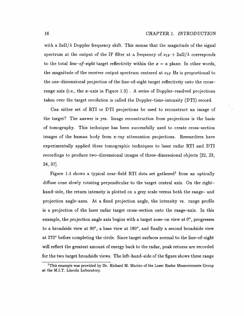
Figure 1.4 shows a typical near-field RTI data set gathered' from an optically
diffuse cone slowly rotating perpendicular to the target central axis. On the right-
hand-side, the return intensity is plotted on a grey scale versus both the range- and
projection angle-axes. At a fixed projection angle, the intensity vs. range profile
is a projection of the laser radar target cross-section onto the range-axis. In this
example, the projection angle axis begins with a target nose-on view at 0°, progresses
to a broadside view at 90°, a base view at 180°, and finally a second broadside view
at 270° before completing the circle. Since target surfaces normal to the line-of-sight
will reflect the greatest amount of energy back to the radar, peak returns are recorded
for the two target broadside views. The left-hand-side of the figure shows three range
1This example was provided by Dr. Richard M. Marino of the Laser Radar Measurements Groupat the M.I.T. Lincoln Laboratory.
16

1.2. RESEARCH PROGRAM
Figure 1.4: A Range-Time--Intensity Imaging Example
17

CHAPTER 1. INTRODUCTION
projection examples. Even though the direct detection intensity data was averaged,
each projection still exhibits the corrupting effects of speckle, shot-noise and receiver
front-end noise. The bottom right-hand-side presents the two-dimensional image of
the cone recovered via tomographic reconstruction techniques applied to the RTI data.
In general, researchers have noted that RTI reconstructions emphasize the outline of
the target, leaving the interior unfilled, while the companion DTI technique produces
silhouette-type images which have smoothed and softened target outlines [37].
The goal of this doctoral research program is to extend the above RTI and DTI
tomographic work to a theoretical analysis of the performance of both laser radar
imaging systems.
First, a realistic model will be developed of a both the RTI and DTI tomographic
imaging systems which includes the effects of operating wavelength, radar-target
geometry, target characteristics, coherent and direct detection, projection processing
and extraction, and finally tomographic reconstruction. Next, the first and second
moment projection statistics will be derived in a manner which takes into account
speckle, photodetector shot-noise and any excess receiver front-end noise. Finally,
these results will be woven together to produce two measures of image reconstruction
quality: the image point spread function (PSF) and the image signal-to-noise (SNR).
These quantities will be the used to interpret previous experimental results.
This dissertation is outlined as follows. The second chapter introduces the reader
to the methods and mathematics of tomography. In preparation for the full laser
radar problem, the third chapter discusses a simple two-dimensional speckle field
tomography problem. Here, we explore the reconstructed image's first and second
moment behavior as well as the image signal-to-noise ratio and resolution. To the
author's knowledge, these results for projections corrupted by speckle noise have not
18

1.2. RESEARCH PROGRAM 19
been investigated in the literature. The fourth and fifth chapters present the RTI and
DTI analysis, respectively. As was the case for chapter three, the results of the RTI
and DTI analysis have not previously appeared in the laser radar literature. Chapter
six compares the theoretical results with previous experiment and simulation. The
final chapter summarizes this research and suggests future work.

2G CHAPTER 1. INTRODUCTION
Chapter 2
The Mathematics of Tomography
Researchers are often faced with representing the characteristics of two- or three-
dimensional objects in image form. For example, a medical doctor searching for a
tumor will find cross-section images of the human body produced by non-invasive
techniques a valuable diagnostic tool. Likewise, the rocket engineer wishing to ensure
the proper distribution of propellant within a solid fuel motor will examine a three-
dimensional representation of motor propellent density. The astronomer may be
interested in imaging the x-ray emission from a supernova remnant or mapping the
electron density of the Sun's corona over the entire solar surface. In all of the above
cases, the two- or three-dimensional image of the object of study cannot be obtained
with conventional photographic or electronic raster scan techniques. Rather, in all
these cases and others, the technique of image reconstruction from projections has
been successfully applied [25]. In this chapter we will study these techniques from
a mathematical perspective. However, we will first overview these techniques by
examining one of the above applications in detail.
The classic illustration of the application of these techniques comes from med-
ical science, where mathematics, computer science and radiology were combined to
21
CHAPTER 2. THE MATHEMATICS OF TOMOGRAPHY
Y'
Projection/
y
:ion
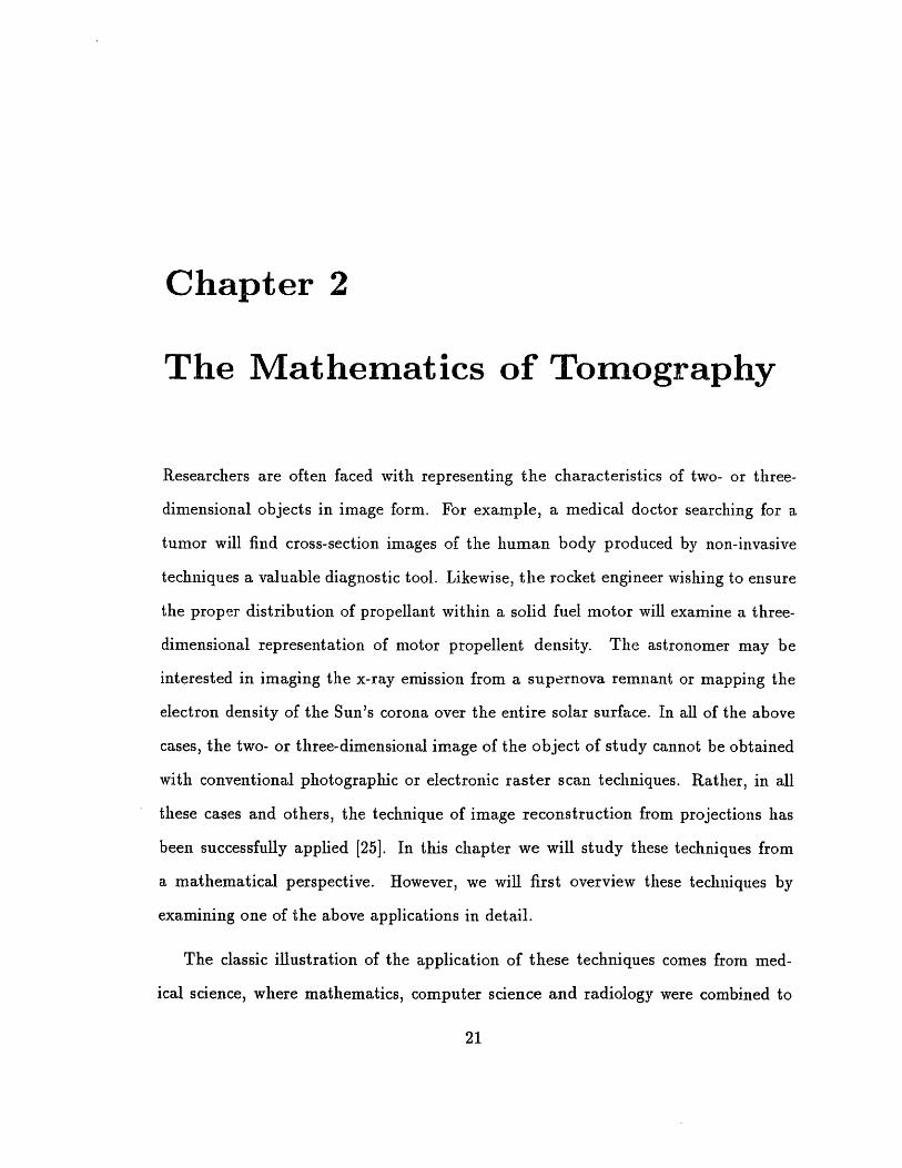
Figure 2.1: Computerized Tomography Geometry.
develop the technology called computerized tomography' (CT)2. The elementary prin-
ciples behind CT are demonstrated in Figure 2.1 [26]. The subject is illuminated with
a collimated sheet of penetrating radiation, usually x-rays. A row of closely spaced
detectors on the far side of the subject measures the amount of radiation exiting the
subject. Assuming that radiation travels in straight lines, the response at any point
on the detector array is an estimate of the radiation transmission from that point
back along a line passing through the subject to the radiation source. The line inte-
gral of the attenuation coefficient f(x, y) over the line L can be extracted from this
1The word tomography is derived from the Greek word meaning "slice." It is used in the contextof medical radiology to describe various methods to image cross-sections of the human body.
2 Computer assisted tomography, computer aided tomography or computed axial tomography(CAT) is also used, as in the term "CAT scanner."
22
K

2.1. THIE RADON TRANSFORM
transmission profile via the relation
Transmission = exp {-Jfdl} (2.1)
In other words, this measurement corresponds to a line integral of the instantaneous
radiation attenuation coefficient. For the given source-detector orientation angle, 0,
the detector array response estimates the collection of line integrals of the instanta-
neous attenuation coefficient f(x,y) lying in the cross-section plane. For this fixed
orientation , this response, denoted as ps(r), is called the projection of f(x, y); it is
a function of the cross-range distance, r. The challenge is to reconstruct the "image"
of the instantaneous attenuation coefficient f(x, y) from the set of projections pe(r)
over all values of the angle .
The collection of all line integrals of a function f(x, y) is called the Radon trans-
form of f. The problem of finding f given the Radon transform of f was solved
mathematically by Radon in his 1917 paper3 . Computer based signal processing al-
gorithms based upon Radon's solution have been applied to the CT problem and
others like it with great success. Motivated by this work, we will survey the mathe-
matical foundations of the Radon transform and derive its inverse in order to apply
the results to Doppler laser radar imaging.
2.1 The Radon Transform
We begin our discussion of the two-dimensional Radon transform by first building a
geometrical framework for this operator. Consider the line in the x-y plane specified
by r = x cos 0 + y sin 9. By rewriting this equation as the dot product r = (, y) ·
3 Radon, J. (1917). UJber die Bestimmung von Funktionen durch ihre Integralwerte Iings gewisserMannigfaltigkeiten. Berichte Sachsische Akademie der Wissen'schaften, Leipzig, Math.-Phys. K.,69, 262-267.
23

CHAPTER 2. THE MATHEMATICS OF TOMOGRAPHY
(cos 0, sin 0) we see that this line is perpendicular to the vector = (cos 0, sin 8)T and
falls a distance r from the origin. This formulation allows us to easily specify any
line in R2 by choosing r and in an appropriate manner. If we restrict E [0, r] and
allow r E R then the space P = R x [0, r] containing the ordered pairs (r, 0) naturally
represents the set of all lines in the x-y plane. Note that P cannot be taken as the
familar polar form because r can be negative.
The two-dimensional Radon transform uses the line integral to map a function on
the x-y plane to a function on the space P. Using the symbol R to denote the Radon
transform operator, the Radon transform of f(x, y) is
[3Rf](r, ) = J dxdy(r - xcos - y sin )f(x, y). (2.2)
For a fixed (r, 0), Rf is simply the line integral of f(x, y) over the line r = x cos 9 +
y sin 9. Thus, the Radon transform decomposes a two-dimensional function into the
set of all line integrals. Note that Rf obeys [f](r, 8) = [Rf(-r, 8 + r) because these
transform values are line integrals traversing the same line in opposite directions, cf.
Figure 2.1.
A few words about notation are in order. We will often consider instances in which
8 is fixed and r is an independent variable. It will be convenient to represent these
cases as [Ref](r), emphasizing the r dependence. This is equivalent to our notion of
the tomographic projection po(r) in Figure 2.1. Furthermore, all single dimensional
Fourier and convolution operations on Radon transforms are understood to apply
only with respect to the variable r. With this convention in mind, we write
[anf I(e) = Jdr e27rjer[fi](r),
and
[g * f](r) = g(r)*[Rsef](r)
24

2.1. THE RADON TRANSFORM
= dr g(r - r)[Ref]().
To familiarize ourselves with these concepts and explore the connection between
the Radon and the Fourier transforms we prove the following theorem known in the
literature as the Fourier slice theorem or projection theorem [27, §II1.1].
Theorem: If e C R then [Rosf](e) = [f](e9)
This theorem states that the single-dimensional Fourier transform of projection Rsf
with respect to the variable r is the cross-section of the two-dimensional Fourier
transform Ff in the direction of 9 = (cos 0, sin 0)T. We begin our proof with the left
hand side.
[ef](e) = J dre-27rjgr Ief](r)
= J dre-' J dxdy(r - x cos S- y sin 9)f (x y)
-= I dxdye-27re(zcos sy sin )f(x, y)
= [f](e cos 0, e sin 8)
= [f](e)-
The reader will recognize that this theorem offers a path to inverting the Radon trans-
form. The function f(x, y) can be recovered from Rf by applying the two-dimensional
inverse Fourier transform to Ff reconstructed from the Fourier slices FRsf for all 9.
However, in practical sampled-data tomographic systems this approach is not highly
accurate and produces image artifacts [27, §V.2]. Rather, in the context of these
systems, researchers have pursued the inverse problem by using the backprojection
operator [27, ch. V]. We now turn our attention to this operator.
25

26 CHAPTER 2. THE MATHEMATICS OF TOMOGRAPHY
2.2 Backprojection Image Reconstruction
To motivate our study of the backprojection operator let us appeal to our earlier
tomography example illustrated in Figure 2.1. Suppose we wish to construct a cross-
sectional image of our subject using the set of projections ps(r). For a given point
(x,y) in the plane, we realize that each projection p(r) at r = x cos + ysin
must contain information about the value of f(x,y). We might try to extract this
information about f(x, y) from our projections by summing over 0 the values of po(r)
such that r = x cos 0 + y sin 0. In essence, we are forming an image by propagating or
"backprojecting" the values of each projection po(r) along the lines r = x cos 0 +y sin 0
across the x-y plane and then summing over . This backprojection operation maps
functions from the space P to the x-y plane (R2 ). For the continuous transmission-
tomography case, the backprojection operator B is defined by [25, §2.2.3]
r
[Bp](x, y) = dpo(x cos + ysin 0). (2.3)
Note that this operator is a dual to the Radon transform in the sense of line-integral
geometry: the Radon transform sums all values of a function f(x,y) along a fixed
line while the backprojection operator sums the values of a function associated with
all lines (r, 0) passing through a fixed point.
2.3 The Inverse Radon Transform
The reconstructed images produced by backprojection incur a smearing-type of dis-
tortion. More specifically, by applying the backprojection operator to the Radon
transform of function f(x,y), it can be shown that [BRf](x,y)- = *f(x, y)
where * signifies two-dimensional convolution [27, Theorem 1.5]. This result, how-
ever, suggests an alternative method for inverting the Radon transform. Taking f,

2.4. SAMPLING AND RESOLUTION
and fy as spatial frequencies, we have via the two-dimensional Fourier transform
[:BRf](f£., If) = f i y2 *f(x, )]
- - [Ff](f Ify).
The backprojected image suffers from a multiplicative radially-dependent distortion
in the frequency domain. Every radial cross-section in the spatial frequency domain or
Fourier slice of the backprojected image has been distorted by a l/loe filtering process
where is the radial spatial frequency variable. Applying the Fourier slice theorem,
we see that this distortion can be eliminated by prefiltering projections pe(r) with the
radial spatial frequency function jIQ. That is, applying the backprojection operator
to F-'[lel x .F[ie(r)] recovers f(x,y) with perfect fidelity. This formulation of the
inverse Radon transform is called filtered backprojection in the literature [26, ch. 7].
Good accuracy and moderate computation requirements make filtered backprojection
a favored starting point for developing algorithms in practical tomographic systems.
2.4 Sampling and Resolution
Modern tomographic systems are sampled-data machines employing digital signal
processing [25, ch. 2]. The above theory must be recast in discretized form to be
relevant. In the semi-discrete case, projections are taken on a finite set of N angles.
Writing this et of projection angles as {n : n = 0, N - 1}, the backprojection
operator becomes
N-1(n+ - O,)pe,(x cosOS + y sin n). (2.4)
n=O
27

CHAPTER 2. THE MATHEMATICS OF TOMOGRAPHY
For N equiangular projections about the half circle (transmission-tomography case)
we haveN-1
P i ,(x COS -n + y sinll n). (2.5)n=O
In the fully-discrete case each projection po,(r) has been sampled along the radial
variable r.
Naturally, the sampled-data model begs questions concerning accuracy and res-
olution. The Shannon sampling theorem answers these questions by specifying the
sampling grid mesh size in terms of the bandwidth of f(x, y). Assume that f(x, y) is
spatially limited (compact) such that f(x, y) is negligible for all (x, y)l>T. Further-
more, assume that the Fourier transform [f](fz, fy) is also negligible in the spatial
frequency domain for (f 2, fy)>b (f(x,y) is b-bandlimited). Note by the Fourier
slice theorem that each projection of f(x,y) must also be spatially limited and b-
bandlimited.
In the fully discrete case each projection is represented by a set of samples along
the r-axis. According to the Shannon sampling theorem, the spatial sampling interval
must be less than the reciprocal of the Nyquist spatial frequency 2b. Therefore, since
each projection is spatially limited, these projections may be fully recovered from a
minimum of 2q+ 1 samples where q = 7Z/(2b)-1 . This sets the sampling requirements
for each projection.
We will now consider the overall two-dimensional sampling requirements for re-
constructing an image of f(x, y) from a set of N projections. Proceeding with a
heuristic argument, this will lead to a lower bound on N in terms of 7R and b.
Assume that we are dealing with the equiangular-projection transmission-tomo-
graphy case, i.e., projections are equally spaced such that ,n, = nlr/N. By the Fourier
slice theorem, the Fourier space of f(x, y) has been sampled in a radial pattern like
28
2.5. RECONSTRUCTION EXAMPLE 29
the spokes of a wheel. These spoke sampling angles in the spatial frequency domain
are identical to the projection angles. Therefore, we must select a radial sampling grid
which approximates the rectangular sampling grid specified by the two-dimensional
Shannon sampling theorem.
In the spatial frequency domain, the sampling mesh size of the radial grid increases
with distance from the origin. The largest mesh occurs at the edge of the frequency
sample space and has a size of 7rb/N. This sample size must be the upper limit of the
corresponding mesh size of the rectangular spatial frequency sampling grid (1/2R)
specified by the two-dimensional sampling theorem. Therefore, for a spatially and
frequency limited function, we have
i rrb> - (2.6)
27Z N
or
N > rq. (2.7)
Thus, if we are required to sample projections 2q + 1 times to satisfy the bandwidth
constraints of f(x, y), then we must use at least 7rq projections to recover f(x, y).
2.5 Reconstruction Example
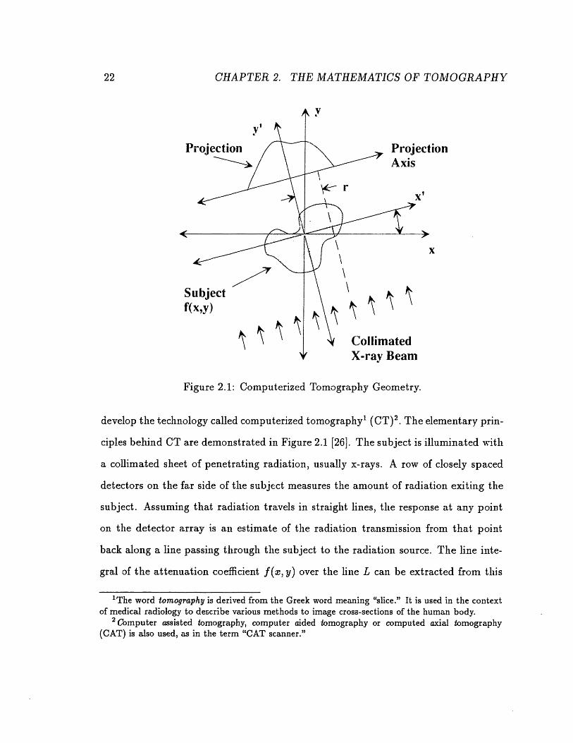
To put these concepts into perspective, Figure 2.2 displays a demonstration of back-
projection and filtered backprojection reconstruction. Transmission projections were
numerically computed at 1° increments for the two-dimensional gray scale phantom
shown in Figure 2.2 (a). Backprojection and filtered backprojection reconstruction
was applied to this set of projections, resulting in the gray scale Figures 2.2 (b) and (c),
respectively. Note that the backprojection reconstruction has a "washed-out" or

CHAPTER 2. THE MATHEMATICS OF TOMOGRAPHY
(a)
(b) (c)
Figure 2.2: Phantom Reconstructions: (a) Original Phantom, (b) BackprojectionReconstruction, (c) Filtered Backprojection Reconstruction.
30

2.5. RECONSTRUCTION EXAMPLE 31
smeared appearance typical of this approach, while the filtered backprojection recon-
struction restores the original phantom with little degradation.

CHAPTER 2. THE MATHEMATICS OF TOMOGRAPHY32

Chapter 3
Two-Dimensional Speckle FieldTomography
As a prelude to an investigation of laser radar tomography, we now examine a two-
dimensional speckle field tomography problem which incorporates some of the aspects
of the more complex laser radar model. Here, we propose constructing projections
of a two-dimensional object by intensity detecting the back-scatter of a penetrating
beam of coherent radiation. Since the field impinging on the detector will be the
superposition of the back-propagated fields from all the scattering sites illuminated
by the probe beam, each projection will be corrupted by speckle-like noise. Our
investigation will center on describing the first and second moment behavior of the
image reconstructed from these speckled projections using semi-discrete tomographic
methods.
3.1 Tomographic Speckle Model
Imagine a transparent test cell filled with a fine aerosol of randomly sized and hap-
hazardly placed particles which scatter light. Suppose we wish to use a narrowly
collimated beam of coherent laser light to determine the two-dimensional distribu-
33
34 CHAPTER 3. TWO-DIMENSIONAL SPECKLE FIELD TOMOGRAPHY
tion of the reflectance density over a plane passing through the test cell. Conceivably,
this could be accomplished by measuring the optical backscatter striking a light de-
tector pointed into the test cell and focused along the laser's line-of-sight. The
laser-photodetector pair could be used to form a reflectance projection of the cell's
contents by sampling along the cross-range axis at a fixed orientation. Projections
could be taken over a number of aspect angles about the plane and combined through
tomographic techniques to form an estimate of the reflectance density. It is the impact
of speckle upon this simplified scenario that we wish to investigate.
Ultimately, we will want to characterize the performance of this imaging scheme in
terms of the resolution and signal-to-noise of the reconstructed density. The statis-
tics of these quality measures will be driven by the aerosol's scattering characteristics.
Therefore, we begin our investigation by specifying the tomographic scanning geom-
etry and the objects's scattering statistics.
Let the circulo-complex Gaussian random process s(x, y) represent the scattering
coefficient of a bounded two-dimensional object resting in the x-y plane. The squared
magnitude of s(x, y) is understood to be the intensity ratio of the scattered radiation
to the incoming illumination at the point (, y). The phase of s(x,y) accounts for
random and uncontrollable variations in the optical round trip path length to the
scattering site.
Assume s(x, y) has the following first and second moment statistics:
* (8(, y)) = o
* ((X 1,yl)8(X2,y 2))= 0
* (8(xl,yl)s9*(2,y2)) = f(xl, Y1)(xl - X2)6(Y1 - Y2)
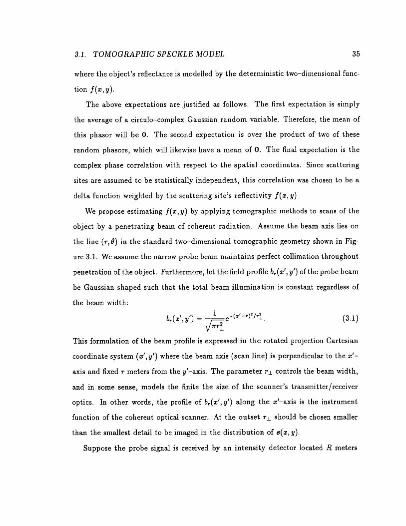
3.1. TOMOGRAPHIC SPECKLE MODEL
where the object's reflectance is modelled by the deterministic two-dimensional func-
tion f(z, y).
The above expectations are justified as follows. The first expectation is simply
the average of a circulo-complex Gaussian random variable. Therefore, the mean of
this phasor will be 0. The second expectation is over the product of two of these
random phasors, which will likewise have a mean of 0. The final expectation is the
complex phase correlation with respect to the spatial coordinates. Since scattering
sites are assumed to be statistically independent, this correlation was chosen to be a
delta function weighted by the scattering site's reflectivity f(x, y)
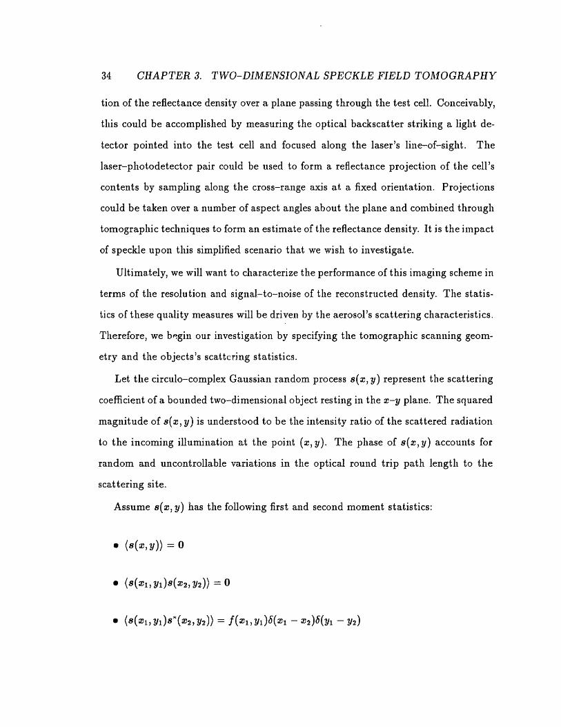
We propose estimating f(x,y) by applying tomographic methods to scans of the
object by a penetrating beam of coherent radiation. Assume the beam axis lies on
the line (r, 0) in the standard two-dimensional tomographic geometry shown in Fig-
ure 3.1. We assume the narrow probe beam maintains perfect collimation throughout
penetration of the object. Furthermore, let the field profile b,(x', y') of the probe beam
be Gaussian shaped such that the total beam illumination is constant regardless of
the beam width:
br(x(', y) e_(=- 1/ (3.1)
This formulation of the beam profile is expressed in the rotated projection Cartesian
coordinate system (x', y') where the beam axis (scan line) is perpendicular to the x'-
axis and fixed r meters from the y'-axis. The parameter rl controls the beam width,
and in some sense, models the finite the size of the scanner's transmitter/receiver
optics. In other words, the profile of b(;', y') along the x'-axis is the instrument
function of the coherent optical scanner. At the outset rl should be chosen smaller
than the smallest detail to be imaged in the distribution of s8(, y).
Suppose the probe signal is received by an intensity detector located R meters
35

TWO-DIMENSIONAL SPECKLE FIELD TOMOGRAPHY
Y'
RelDis
7
Object s(x,y)
x
r
(r, )
Figure 3.1: Two-Dimensional Speckle Tomography Geometry.
36 CHAPTER 3.
.,
on

3.2. PROJECTION STATISTICS
from the x' axis. Assuming negligible beam attenuation, we can write the complex
signal field envelope at the infinite extent detector as
R(r, 9) = j j dx'dy's(x(x', y'), y(x', y'))br(x', y)e2jk(R+y') (3.2)
where k 27r/A is the wavenumber. Note that we have reformulated the scatter-
ing distribution s(x(x',y'),y(x',y')) upon the rotated coordinate system (',y') by
specifying the following transform:
x(x',y') = x'cos - y'sin
y(x', y') = ' sin S + y' cos 9.
Since individual points lying in the probe beam's path reflect waves back to the
intensity detector with random phase, the output signal will be corrupted by speckle
noise.
3.2 Projection Statistics
Using the fact that IR(r, 0)12 = R(r, 0) R*(r, 9) where the * denotes complex conju-
gate, the first moment of the detector response is then
(IR(r,9)12 ) KjdL l
jroo J dxdyls*(x 2(x,, y), y2(x, y'))b,(x, yl)e2(R)
Exchanging the expectation and integration operators, and substituting f(x, ,yl)
6(X1 - x 2) (Y1 - Y2) for the reflectivity correlation (s(X 1,yl) 8*(X 2 ,Y2)), we find
0co 1) = 1 _(_/,1(3.3)( (r)Joo d'ldy f(x l(l 1 ), (x y)) --r/2e (33)f oo ft
37

38 CHAPTER 3. TWO-DIMENSIONAL SPECKLE FIELD TOMOGRAPHY
Recalling that r is small compared to the object's spatial detail, we make the ap-
proximation --;l ;e-2(\-')' /'L 1 8(xi - r) resulting in
roo poo 1(lR(r,)12) dxldylf(l(lyl)yl(xll) ) 6(x -r)
dyl fi ((r, y')y1i(r y))
1 1[Rf](r, ).
Thus, for small r, (IR(r,9)12 ) behaves like the Radon transform of the object's
reflectance f(x,y) within a scale factor. Thus, within an approximation, it seems
reasonable to regard (IR(r, 0)12) as a projection of the scattering object s(x, y). While
this result is intuitively pleasing because it makes physical sense, this analysis can be
extended to explicitly include the effects of the Gaussian beam profile (instrument
function) upon the Radon transform formulation.
Intuition tells us that features smaller than the probe beam's width will be lost
or suffer from a smearing type of distortion. Starting with (3.3) and the definition of
the Radon transform, it is easy to back out the result
(JR(r, )12) = - g(r) * [f](r) (3.4)V22rr 2
where g(r) has the Gaussian form
g(r) = e-2r2r (3.5)
Thus, each projection (R(r, 0)12) is proportional to the true Radon transform [Ref](r)
convolved with a narrow Gaussian window. Using the fact that [h](r) * [Ref](r) =
[!a(x~(z, y) f(x, y))](r) we realize that we can extend the above result to
([R(r, )12) = R[g(,y) * f(x, y)] (3.6)2 7rr

3.2. PROJECTION STATISTICS
where
g(r) = [Re{g(x,y)}](r) (3.7)
and
g(x, y) 2= e_2(-/ (3.8)
Thus, the set of projections IR(r, t)12 formed by the above "narrow Gaussian-beam
transform" correspond in the mean to the true Radon transform of the convolution of
the reflectance f(x,y) and a function g(x ,y) determined by the probe beam profile.
The small-scale smearing caused by this effect will fundamentally limit the resolution
of any reconstruction algorithm applied to R(r, 0)12.
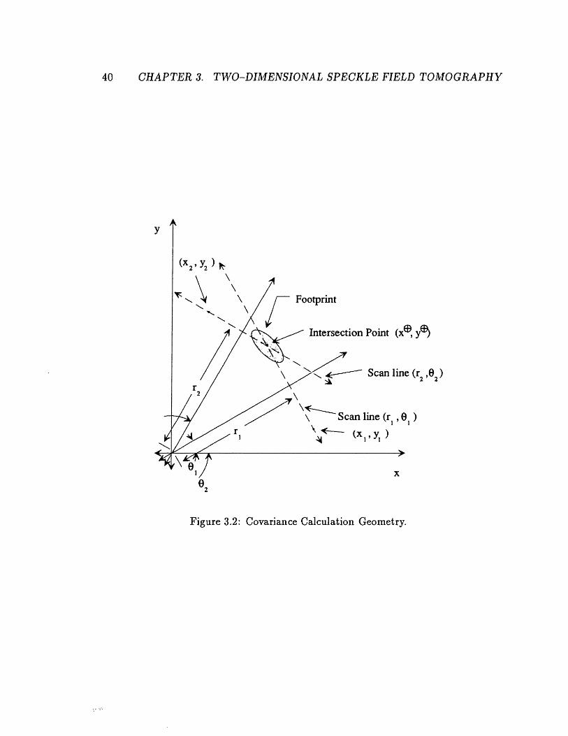
In addition to the first moment of R(r, 8)12, it is of interest to characterize the
cross-correlation between the received signal fields, R(r1,t ) and R(r 2, 92), fol the
two scan lines (r1, 81) and (r2, 82) respectively. That is, we wish to compute the cross-
correlation (R(rl, 1)R*(r 2, 92)) in the semi-discrete case. As shown in Figure 3.2,
this expectation will be largely determined by the values of the reflectance f(x,y)
within the "footprint" formed by the intersection of the two narrow probe beams
along the scan lines (rl, 8) and (r2,02). This realization requires the consideration
of two distinct geometrical cases.
First, suppose the projection angles 81 and 2 are equal. In this case, the two
scan lines are parallel and the expectation will be nonzero when there is significant
overlap between the two narrow probe beams (i.e., r _ r2 ). This expectation can be
approximated by
(R(rl, )R* (r2, ))
= t j dxdy8(xi(x, yl), yi(,y'))br(Xt Y)e
j I dxdy8*(X 2( , y'), y2(X2, y))br(X2, y2)e-i( i) (3.9)
39
TWO-DIMENSIONAL SPECKLE FIELD TOMOGRAPHY
(xy(X2 Y2
I.-,
'.1
e (r 2 '02 )
x
Figure 3.2: Covariance Calculation Geometry.
40 CHAP TER 3.
I)
\ - (x , y,

3.2. PROJECTION STATISTICS
,.,,.,,,,,.,roo ~Df d f_ 1(r2 rl)21 2ri 2 dxl dy"O f(x1 ( 1 y, Y1 (z ,A)) e-2(z, -(r2+rl)/2)2/r2i
-0 0oo -0 0 rr
1 _(r2_rl)2/2r [f](2 + r12irr 2 , ), (3.10)\/2 7rrl 2 '
where the approximation is obtained by retaining the r small condition as before
and passing to the Radon transform.
Second, consider the case when the two projection angles are unequal. In this
scenario the two scan lines (rl, 1) and (r2, 2) always intersect at a single point
(x@,y 9) in the x-y plane. The coordinates of this intersection point are dependent
upon the values of (rl,0 1 ) and (r 2,02 ) and take the values:
1
xe°(ri,' 1;r 2 92) = - )(rl sin(02) - r2 sin(01)) (3.11)
y(ri, 1;r2, 2 ) = sin( _ )(-rl cos(02) + r2 cos(91)). (3.12)
Beginning with equation (3.9), the expectation can be manipulated into a compli-
cated double-integral on a rotated coordinate system centered on the point (Xz, y@)
with an integrand of f and a complex phase factor windowed with the Gaussian pro-
files of the two probe beams. At this point, if we assume that the most significant con-
tribution comes from the region of the intersection footprint of the two narrow probe
beams, then the two beam profiles can be replaced with a single a two-dimensional
Gaussian window centered on (xe, y@) with major and minor axis lengths a function
of the angle of attack, 2 - 1, of the two scan lines. Again, assuming r is small
and f(x, y) varies slowly within the Gaussian window patch, then the double-integral
may be approximated by the value 2f(zx(rl, 01; r2, 02), y(rl, 01; r 2, 02))/ sin(8 2 -1)
times a complex phase factor. The factor of 1/I sin(02 - 01)1 accounts for the change
in the size of the footprint area as the scan line angle of attack varies. Therefore, for
41
42 CHAPTER 3. TWO-DIMENSIONAL SPECKLE FIELD TOMOGRAPHY
non-identical projection angles, the cross-correlation is approximated by
(R(rl, 01)R'(r 2, 02)) = 2Cf(xz(r, 01;r 2, 02), y9(r, 1 ; r2, 02))/1 sin(0 2 - 1)1l (3.13)
where C is a complex phase factor. The details of this calculation are disclosed
in Appendix A. This result is intuitively pleasing because it formulates the cross-
correlation in terms of the scanning geometry. As the angle of attack between two
projections decreases, the cross-correlation increases because the probe beams cover
a growing common region within the scattering object.
3.3 Backprojection Image Statistics
Let us now turn our attention to the first and second moments of the reflectance image
formed by applying the discrete backprojection operator to the set of magnitude
projections R(r,9)12 of s(x,y). In the semi-discrete case let Abp(x,y: N) be the
backprojected image formed by using N equiangular projections. Thus
Abp(x,y : N) = E - R(c (3.14)n=O snn, n)
The semi-discrete mean image is then
1 N-1
(Ab(x,y: N)) i= N- 1 [9(XY)* f(XY)] (3.15)
It would be instructive to write this result in the form of f(x,y) convolved with a
point-spread-function (PSF). By setting f(x, y) = 8(x - xo,y - y,) and using the
property R9[f*g] = Rf f*sog it is easily shown that (3.15) represents a shift-invariant
linear system. Thus, we may alternately write
1(Ap(x,y : N)) = V .f(:x,y) *Gbp(x,y : N) (3.16)
2irr(

3.3. BA CKPROJECTION IMAGE STATISTICS
-o1 I 1-
Figure 3.3: Normalized Mean Backprojection Image PSF, Gbp(, y: 4)
where
N-1 7F
Gbp(,y: N) = i[Rng(',y')](xos Nn + y sin 7n)n=0
N-i 1~r a-o 1 -2(,cos n+y sin n)2/ (3.17)
= x~ irri/2N(3.17)
represents the N dependent PSF of the mean image. Figure 3.3 shows a surface plot
of the normalized PSF for N = 4 projections.
As N grows without bound, the semi-discrete backprojection case approaches
the continuous case as a limit. Define Abp(x, Y) to be the image produced by the
continuous backprojection operator:
Abp(x,y) = B[IR(r,0)12 ]
43

44 CHAPTER 3. TWO-DIMENSIONAL SPECKLE FIELD TOMOGRAPHY
= jo d R(r, o)12.
The mean of Abp(x, y) is found to be
(Abp(x, y)) = ( [R(r, )12])
= S(IR(r, 0)12)
= 2_r_ 8r[B[g(, y) *f(x, y)]
g (, Y) f(z, Y) (3.18)
Thus, the point-spread-function (PSF) of the mean of this narrow-beam tomographic
scheme under backprojection reconstruction is g(x,y) * ( 2 + y2)-1/ 2. Therefore,
continuous backprojection reconstruction alone cannot fully resolve f(x,y) within
the limitations imposed by the narrow-beam approach.
The reconstructed image noise strength is measured by the image covariance.
Let KAAbp(X1,Y1;x2,2 : N) designate the covariance of the image Abp(,y : N)
formed by semi-discrete backprojection. Using complex-Gaussian moment factoring
the covariance may be simplified to the following form:
KAAbp (x1, Y1; 2, Y2 : N)
- NZ E i KRn(x cos n + Yi sin n)R* i(X2 cos i + Y2 Sinl i)n=O i=O
(3.19)
This result is equal to the summation of the magnitude-squared values of the cross-
correlation between the received signal fields R corresponding to the scan lines (rn, 9n)
and (ri, Si)
Consider the case of identical indices within the double-summation. The dou-
ble summation will collapse to a sum of the magnitude-squared equiangle cross-
3.3. BACKPROJECTION IMAGE STATISTICS
correlations. Itence, this component of the covariance becomes
a2 N-1 i7r - 2- 2 exp -[(X2
[,f] 1 2 cos n +7LJfV (~ cos -n +k2 N
- x,) cos N n + (Y2 - Y) sin Nn] /r2}
Y2 + Yi
2
7 7rsill -n - )
For non-identical indices we have the case of unequal projection angle cross-cor-
relations within the double-summation. Thus, the semi-discrete covariance may be
approximated by the sum of these two results:
KAAb(xi, Yl; 2, Y2 : N) a-2 N-1 - E 2 exp -[(X2
N 2 27Ir exp
[f]2( X2 + c +
- X,) cos Nn + (Y2 - Y1) sin n]2/r }
Y2 + Yi
2
X
sin -n, Nn +
7 2 N-1 N-1
N_2 On=O i=O,i4n
4
sin2 (n- i)Y\""(3.20)
where
ar = xicos 7i+yrsin ',rl = Xi cos -i + yl sinai,N N
r .7rr = x2 cos -n + Y2 sin n.N N
The reconstructed image variance varAA (, y : N) can be easily obtained from
the above covariance expression by setting (l,yl) = ( 2,Y 2) = (,Y). Under this
restriction the point ((rl, 01;r2, 02), y(ril, 01;r2,02)) reduces to (xl, y) giving
varAA~ (X, y: N) N2 E-n=O
2R [f] 2 (X27rNiN-
7r 7r 7rcos -n + y sin -n, n)N N N'
45
x
~f2(X r . 7r'(2(r, N,; r2, -n), y"(r,N N
7r . 7r' z; r 2 , _n)),
(3.21)
(3.22)
2 N-1 N-1 4
N2f (z,y) E sin2 (n-i)n=O i=O,i54n
+
(3.23)
46 CHAPTER 3. TWO-DIMENSIONAL SPECKLE FIELD TOMOGRAPHY
Hence, the variance of the reconstructed image consists of two terms, one proportional
to f 2 (x, y) and the other proportional to the backprojected image of the square of the
Radon transform of f(x, y).
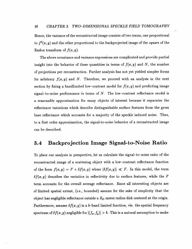
The above covariance and variance expressions are complicated and provide partial
insight into the behavior of these quantities in terms of f(x,y) and N, the number
of projections per reconstruction. Further analysis has not yet yielded simpler forms
for arbitrary f(x,y) and N. Therefore, we proceed with an analysis in the next
section by fixing a bandlimited low-contrast model for f(x, y) and predicting image
signal-to-noise performance in terms of N. The low-contrast reflectance model is
a reasonable approximation for many objects of interest because it separates the
reflectance variations which describe distinguishable surface features from the gross
base reflectance which accounts for a majority of the speckle induced noise. Thus,
to a first order approximation, the signal-to-noise behavior of a reconstructed image
can be described.
3.4 Backprojection Image Signal-to-Noise Ratio
To place our analysis in perspective, let us calculate the signal-to-noise ratio of the
reconstructed image of a scattering object with a low-contrast reflectance function
of the form f(x, y) = F + Sf(x, y) where If(x, y)I < F. In this model, the term
Sf(x,y) describes the variation in reflectivity due to surface features, while the F
term accounts for the overall average reflectance. Since all interesting objects are
of limited spatial extent, (i.e., bounded) assume for the sake of simplicity that the
object has negligible reflectance outside a RD meter radius disk centered at the origin.
Furthermore, assume 6f(x, y) is a b-band limited function, viz. the spatial frequency
spectrum of Sf(a, y) negligible for (f,, fy)l > b. This is a natural assumption to make

3.4. BACKPROJECTION IMAGE SIGNAL-TO-NOISE RATIO
since most objects of interest have surface feature variations which are smooth on a
small enough scale. We will find it useful to let Xf designate the indicator function
for f(x,y), i.e.,
Xf(X y)= = 0 iff f(x,y)=0 (3.24)1 otherwise.
Thus the indicator function for our scattering object is a RD meter radius unit height
disk.
The signal-to-noise ratio (SNR) under semi-discrete backprojection reconstruc-
tion is defined as follows
SNR = [mean reconstructed signal]2
mean squared noise strength
,. [ f(x, y) Gbp(x, y : N)]2
varAAbp(, Y : N)
(6f(x, ,) * G(x, y N))2NF2 Eno [rnXf (X1 COS n + y, sin n) +
N227r IF2 n=O i=Oi n sin2 (n-i)
where we have used f(x, y) - F in the expression for the variance. For N > 10 the
double summation in the denominator can be approximated by 4N3 giving
SNR f(x, y) * Gbp(x, y: N)]2 (3.25)72 F2 -N-lX - f2(Xl COS 2
N2 F2 E=l[ n xfJ2( 1 cos n + yl sin n) + 2rrN2 4N3F2
Recall that Sf(x, y) is b-band limited. Therefore, the appropriate number of projec-
tions to fully recover Sf(x, y) is rq where 2q + 1 is the number of points specified by
the one-dimensional Shannon sampling theorem for the proper sampling and recovery
of any one projection. For a RD meter bandlimited disk,
q = (disk radius (m)) + (sampling interval (m))
= RD (m)/(2b)-1(m)
= 2bRD (dimensionless).
47

48 CHAPTER 3. TWO-DIMENSIONAL SPECKLE FIELD TOMOGRAPHY
Thus, we set N = 27rbRD. Furthermore, we fix the beam width equal to the size of the
smallest detail on the bandlimited disk, i.e., r = 1/b. Therefore, the signal-to-noise
ratio becomes
SNR F2 (ZN- [6sf(x, y) * Gbp(x, y: N)]2
2bZ (n-° N[,RXxf ](x1 cos n + y sin n) + 7r4)
21-r f 2 f(x, y) * Gbp(x, : N)] 2/ITr (3.26)A computer was used to calculated the above NR quantity for a RD = 1 meter(3.26)a2 (EN- -]IrCOS 327r4 R2
F 2 ( ~ N-n=0[ ,X]2(=O co fn d y sin 'rn) - N-~- 3 "
Note that the squared term in the numerator and the summation (backprojection)
term in the denominator both approach finite limiting values as N grows without
bound.
A computer was used to calculated the above SNR quantity for a RD = meter
radius disk. During the calculation, the bracketed term within the numerator was
approximated by Sf(x, y) times the area under Gbp(x, y: N). This is valid under our
assumption that b is less than or equal to the spatial bandwidth of Gbp(z,y: N).
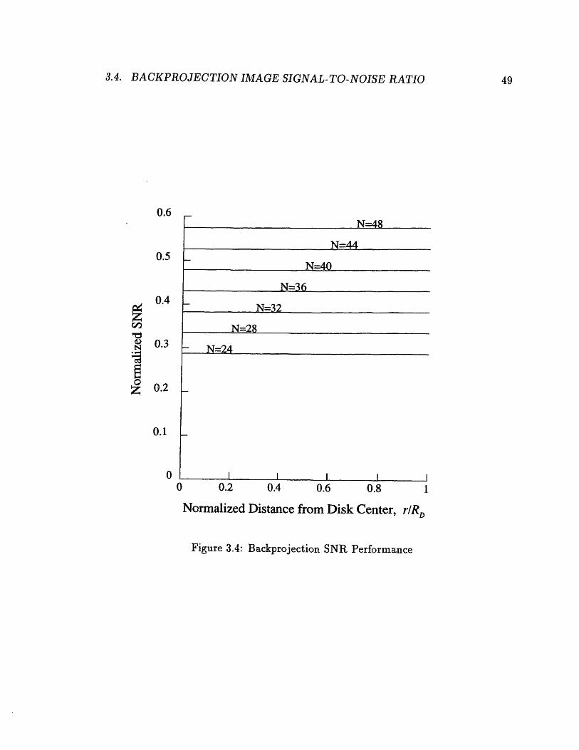
The resulting SNR was found to have a radial profile which did not vary in respect
to rotation about the disk center. Therefore, Figure 3.4 presents a radial plot of
(3.26) normalized by the factor f 2(x, y)/F 2 for a family of N values. For a fixed
number of projections the above SNR equation scales independently with respect to
RD. Therefore, this set of curves can be interpreted as the normalized SNR of the
backprojection reconstruction of a RD meter disk where the abscissa scale is now in
terms of r/RD.
Note that the SNR performance is nearly constant versus radial distance from
the center of the disk. Thus, the disk image SNR is proportional to the number
of projections required to fully reconstruct f(x,y) under our bandwidth constraint.
This result stands in contrast to ordinary speckle-imaging systems which coherently
combine measurements during pixel formation, achieving SNR's equal to one [28].
3.4. BACKPROJECTION IMAGE SIGNAL-TO-NOISE RATIO 49
N=48
N=44
N=40
N=36
- N=32
N=28
- N=24
I I I . I0 0.2 0.4 0.6 0.8 1
Normalized Distance from Disk Center, rRD
Figure 3.4: Backprojection SNR Performance
0.6
0.5
0.4
0.3
0.2
z̀a$v;9Ir
0.1
0

50 CHAPTER 3. TWO-DIMENSIONAL SPECKLE FIELD TOMOGRAPHY
However, even in our case at 5f 2(, y)/F 2 = 1, we do not obtain a unity SNR until
N > 84. Considering the slow SNR rise vs. N, and the poor resolving power of
backprojection reconstruction, this tomographic speckle-imaging technique offers rel-
atively substandard performance, even for the larger sized projection sets of N - 200,
the typical number of projections recorded by a commercial CAT scanner.
3.5 Filtered Backprojection Image Statistics
Now consider a similar analysis for semi-discrete filtered backprojection processing.
In this case we will prefilter every projection before performing the backprojection
sum. Let Afbp(x,y: N) be the backprojected image of the reflectance formed by
using N equiangular filtered projections. Thus
Afb (,y: N) =N-1
N [-1 {II x .'F[jR(r', Nn)I2]}] (x cos Nn + y sin Nn) (3.27)n=-
where the expression within the outer brackets represents the filtered backprojections
as a function of r, and r is then set equal to x cos Nn + y sin Nn under the back-
projection sum. In order to simplify the notation during further discussions, let the
symbol 'H[p(r)] denote the filtering operation F-'{lel x F[p(r)]. The semi-discrete
mean image is then
(Afbp(x, y: N)) - x
N-1E Nle X [[Rn(g(', ) * f(x', y'))](r' )] }]( cos n + y sin n)
N-1= E. ~Y7[R~-n(9(x', y') * f(X', y'))]( cos Nn + y sin gn). (3.28)
n=0
As in the case of simple backprojection, the mean image PSF Gfbp(X,y : N) for
semi-discrete filtered backprojection can be calculated. Thus, we may alternately

3.5. FILTERED BACKPROJECTION IMAGE STATISTICS
write
(Af bp(x, y: N)) = ff(, y) * Gfbp(x, y: N) (3.29)
whereN-1
Gfbp(x, y: N) = E Rgf( cos -n + y sin n) (3.30)n=O
where the function gf(r) is equal to
gf(r) = [[Rng(xy)](r)]
= '-L {(e x [(1/ r/2) e 2(r)-] } (3.31)
The function gf(r) is plotted in Figure 3.5. The width of the central lobe deter-
mines the fundamental resolution of the filtered backprojection image reconstruction
scheme. Since filtered backprojection is one solution to the inverse Radon transform,
as N grows large and we pass to the continuous case, the PSF for the mean image
must be g(z, y) defined in equation (3.8) within a scale factor. Thus, the fundamental
resolution cell size is equal to the width of g(x, y) which is physically determined by
the scanning instrumentation.
The filtered backprojection image noise strength is measured by the reconstructed
image covariance. Let KAAfbp(Xl, Yl; 2 , Y2 : N) designate the covariance of the image
Afbp(x, y: N) formed by N equiangular semi-discrete filtered backprojection recon-
struction. Recalling that the filtering operation 7- is performed with respect to the
radial projection variable r, the filtered backprojection covariance may be written as
KAAb, (Xl1, YI;x2, Y2: N)
21rrT N no Nr2 [ e-(r2-rl)2/T[Rf]2(r 2 ' r )]
(X1 COS n + Yl sin N n) (X2 COS n + Y2sin n) +NN N N
51

52 CHAPTER 3.
1
0.8
N~0Z
0.6
0.4
0.2
0
-0.2
-0.4
TWO-DIMENSIONAL SPECKLE FIELD TOMOGRAPHY
I I I I I I-4 -2 0 2
Normalized Radial Distance,
(a)
.-.
(b)
Figure 3.5: Filtered Backprojection Mean Image PSF (a) gf(r), (b) Gfbp(x, y: 4)
4
r/r
6-0

3.6. FILTERED BACKPROJECTION SIGNTAL-TO-NOISE RATIO
N2 i N si (n i) [f [f2((rl, -i;r 2, in),y y(rl, -i; r2, Nn))n= s i=-,i)n nL - (
(Xl cos n + yl sin n) (2 cos Ni + y2 sin i) (3.32)N N NN
where the operators 7-, and 7tr2 filter with respect to the variables r1 and r2 re-
spectively. This expression is valid because the expectation, backprojection and X
operators are all linear. Thus, the prescription for finding the covariance is to filter
the expression within the inner brackets with respect to variables r and r2 and then
replace r and r2 with the proper cartesian coordinate expandb:on before performing
the sums. The variance of Afbp(x, y: N) may be obtained from the above expression
by setting (i,yi) = ( 2, Y2) before computing the sums.
The above covariance and variance approximations are complicated and provide
little insight into their behavior as f(x,y) and N vary. Further analysis has not
yielded a simpler form for arbitrary f(x,y) and N. Therefore, as in the case with
backprojection reconstruction, we have proceeded with the SNR performance analysis
of a bandlimited low-contrast disk-like scattering object.
3.6 Filtered Backprojection Signal-to-Noise Ra-tio
For the reasons cited in §3.4, let us calculate the signal-to-noise ratio of a filtered
backprojection image reconstruction of a RD meter radius disk with a low-contrast
reflectance of the form f(x,y) = F + Sf(x,y) where 1f(x,y)J << F. As before, let
Sf(x, y) be a b-band limited function. Thus, the SNR under filtered semi-discrete
53

54 CHAPTER 3. TWO-DIMENSIONAL SPECKLE FIELD TOMOGRAPHY
equiangular backprojection reconstruction is:
SNR - (mean reconstructed signal)2
mean squared noise strength
9-(8f(x, y) * Gfbp(x, y : N))2
varAAfbp(x, y: N)1 (Sf(x, y) * Gfbp(2, y: N)) 2
2 2XTZ (3.33)F2 27rrI VarAAfbp(X,y: N)/F 2
where the second term in the above product represents the SNR of a reconstructed RD
meter radius unit-height disk. This quantity has been numerically evaluated under
our bandwidth restriction of b = 1/rl and found to be radially symmetric about the
center of the disk within the resolution capabilities of the calculation. Figure 3.6
shows a radial plot of this second term for a family of N values. Each plot has been
normalized by f 2(x,y)/F 2 and the height of the filtered backprojection impulse
response Gfbp(,y : N) to facilitate direct comparison to the backprojection results
of §3.4. The b-bandwidth restriction has been enforced by windowing the 1/1pl spatial
frequency filtering with a Gaussian function centered on the frequency origin. Again,
we have used the relation N = 27rbRD to relate the number of projections to the
image bandwidth. Since (3.33) scales independently with the disk radius for a fixed
N, Figure 3.6 can be interpreted as the normalized SNR of a filtered backprojection
reconstruction of a RD meter disk where the abscissa scale is in terms of r/RD.
It is intuitively pleasing that the SNR increases with the number of projections in
light of projection signal processing which would tend to enhance high frequency noise.
Observe that as the number of projections increases, a peak appears to grow in height
at the edge of the disk. This seems to indicate that image quality is better at the
edge than in the disk interior. However, this phenomenon may be a phantom caused
by a large spatial frequency filter response at the disk edge drop-off. Furthermore,
slight SNR variations appear near the disk center as the number of projections rises

3.6. FILTERED BACKPROJECTION SIGNAL-TO-NOISE RATIO
0 0.2 0.4 0.6 0.8 1
Normalized Distance from Disk Center, rIRD
Figure 3.6: Filtered Backprojection SNR Performance
0.3
0.25
Zlcl0N
Ig
0.2
0.15
0.1
0.05
0
55

56 CHAPTER 3. TWO-DIMENSIONAL SPECKLE FIELD TOMOGRAPHY
0.6
0.5
z 0.40 3
N 0.3
O 0.2Z
0.1
0
BACKPROJECTIONRECONSTRUCTION
LEREDBACKPROJECTIONRECONSTRUCTION
I I I I I
20 25 30 35 40 45 50NUMBER OF RECONSTRUCTION PROJECTIONS
Figure 3.7: SNR Performance Comparison
above 40. This is believed to be caused by resolution limitations within the numerical
calculations.
Figure 3.7 plots the normalized disk center SNR for both the backprojected and fil-
tered backprojected reconstructions. Over the set of N, both reconstructions achieve
SNR's of less than one, with filtered backprojection performance lying approximately
8 dB below the backprojection curve. Furthermore, a linear extrapolation carried
out upon the central region of the filtered backprojection curve indicates that a unity
SNR will be obtained for N ~ 480, a value much larger than the corresponding back-
projection case. However, since both reconstructions have differing resolutions, this

3.6. FILTERED BACKPROJECTION SIGNAL-TO-NOISE RATIO
is not a fair comparison. For a non-random Sf(x, y), the image mean squared error
(MSE) for both reconstruction techniques breaks down into the variance of the recon-
structed low-contrast reflectance, 6f(x, y), plus the square of a second bias term. The
Sf(x,y) variance is inversely proportional to N, while the bias measures the depar-
ture of the reconstruction PSF from a delta function; the ideal imaging system PSF.
Making the comparison on this basis, the backprojection reconstruction bias term is
larger than the corresponding filtered reconstruction term because of the relatively
poor backprojection reconstruction resolving power, while the backprojection recon-
struction f/(, ,y) variance is smaller than the corresponding filtered reconstruction
contribution because, in this latter quantity, spatial projection filtering emphasizes
high frequency noise. Therefore, the SNR advantage of backprojection reconstruction
comes at the expense of much poorer resolution (cf. Figure 2.2 (b) and (c) and also
[24, Figure 18.]).
57

58 CHAPTER 3. TWO-DIMENSIONAL SPECKLE FIELD TOMOGRAPHY

Chapter 4
RTI Tomographic ImagingPerformance
We now turn our attention to the range-resolved laser radar tomography problem
originally outlined in chapter 1. In this scenario we use a direct detection laser
radar to illuminate a spinning target to obtain a fixed number of range resolved
returns which correspond to a set of projections of the target reflectance onto the
range axis. Tomographic techniques will then be applied to this semi-discrete range-
time-intensity (RTI) record of the target revolution to reconstruct a two-dimensional
reflectance image of the three-dimensional target. The goal of this investigation is to
examine the performance of this imaging technique.
The discussion in this chapter is organized along three main thrusts. First, we will
introduce the concepts necessary to build a mathematical signal model of the imag-
ing problem which will allow us to compute the first and second moments of the re-
constructed image. This model incorporates radar-target geometry, electromagnetic
propagation, target characteristics, direct detection and finally, tomographic image
reconstruction. As in most mathematical models of complex physical processes, we
are often forced to adopt approximations during the analysis which degrade accuracy
59
CHAPTER 4. RTI TOMOGRAPHIC IMAGING PERFORMANCE
but provide useful explicit closed-form performance predictions. While such is the
case here, we nevertheless hope to develop a theory which will qualitatively satisfy our
curiosity concerning the issues and interpretations of the reconstructed RTI images.
Here, our ultimate goal in modelling is to quantify the reconstructed image quality
in terms of resolution and SNR-like measures.
The second section deals with the calculation of the first and second moments
of RTI projections. The emphasis in this chapter will be on the discussion of the
assumptions and approximations behind the calculations and a presentation of the
results along with their proper interpretation. Full disclosure of every step of the
computations is made in Appendix B along with a detailed discussion justifying all
assumptions. While this necessitates some duplication in the presentation, it was felt
that the reader of this chapter should be spared from the seemingly daunting stream
of changes of variables, integrations and transformation operations required to obtain
the sought after signal covariances.
In the final section, the results of the two previous sections will be woven together
to produce two measures of the reconstructed image quality. The image resolution
will be derived from the projection mean, while the image SNR will be fashioned from
both the projection mean and variance. A discussion comparing these results with
previous experimental results and the companion DTI results of the next chapter will
be the scope of a later chapter.
As we begin the process of constructing the RTI imaging model, the most difficult
aspect to conceptualize is the specification of a target with arbitrary shape, reflectance
and roughness. Therefore, we step back from this general situation and begin by fixing
the target shape as spherical. While this action limits the results to a specific case,
we still should obtain a qualitative description of the performance in terms of the
60

4.1. RTI TOMOGRAPHIC IMAGING MODEL
laser radar design parameters.
4.1 RTI Tomographic Imaging Model
In this section we will construct a model of the RTI imaging system. Model elements
and issues will be discussed in the order the are visited by the pulse emitted by
the transmitter, beginning with the transmitter beam modulation and propagation,
and then, target characterization, direct detection and finally post-detection image
processing.
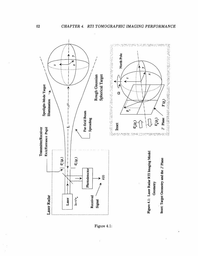
Many features of the direct detection laser radar model are shown in Figure 4.1.
The model features a laser radar in which the transmitter and receiver apertures
share the same optical axis. We assume the spherical target is at a constant on-axis
position in the radar's optical far-field at a distance of L meters from the transmitter
aperture. The rigid target is centered at the origin of the target coordinate frame
(., y, z) and spinning about the z-axis at a rate of f2 radians/second. On the scale
of the transmission wavelength A, the microscopic surface variations of the target are
large and random in nature.
This geometric model is motivated by the tomographic imaging of a rotating
satellite from a ground- or space-based laser radar. In this scenario, targets typically
1-10 meters in size spin from 1-60 revolutions per second at range from the radar
which can easily exceed 100,000 meters.
4.1.1 Transmitter Beam Propagation
The process of measuring a set of target range projections begins with the trans-
mission of a train of short-duration optical illumination pulses. The optical source
within the transmitter is a laser which emits a spatially- and temporally-coherent
61
62 CHAPTER 4. RTI TOMOGRAPHIC IMAGING PERFORMANCE
:· !z' .' ::...
...::
:... ...a'0, :'..
~~~~~~~~~~~~~~~~~~~~~~~~~~~~~~~~~:. .:: ::
a.
f ;Sa~~~~~~~~'- ~: ..i , · i: > , ·: . . s. ;, ·:~ , , : *·· :,,· ·- ~ ... ,,{:· ,}- .·i:
: _)
08 bO
a aI;'. E X~~~~~~~r
: W~~~~~~~~~r
Figure 4.1:
a
0
a-
··:.
.·c.
··.·:··.. ··;·.·.·
··�
;:::·'· ·-'
·":;i·'' '
�::·:·.
· ·.·:.·;
�·'
·.;·
�
.·...
·;.
·.· "'`"'
4.1. RTI TOMO GRAPHIC IMAGING MODEL
linearly polarized monochromatic beam at the fixed frequency of vo = c/A. The nth
pulse arriving at the target at time tn is formed at the transmitter exit pupil by
amplitude modulating the electric field of the +y-axis traveling wave by the envelope
VS(t - (t - L/c)). The retarded time adjustment term L/c accounts for the time-
of-flight from the laser radar to the target. The envelope s(t) has a peak value of
unity at t = 0 and a very narrow width of T seconds. Since the range resolution will
be proportional to the pulse spatial depth, cT, systems producing useful resolution
·will require T to be less than a nanosecond for meter sized targets.
Under the linear polarization assumption, we may represent the electromagnetic
field strength of the nth pulse exiting the transmitter pupil by using the complex
scalar description [29, Chapter 3]
Ut(p1, t) = PT T(P1) (t - (tn - L/c)) (4.1)
where Ut(pi, t) is' proportional to the complex scalar envelope of the outgoing electro-
magnetic wave, PT is the peak transmitter power and T(1i) is the normalized com-
plex transmitter spatial mode (antenna pattern) within the exit pupil plane spanned
by the two-dimensional reference vector , i.e.,
/ d)p l (#)l2 = 1. (4.2)
Pupil
Therefore, the optical power launched to the target in the nth pulse is equal to PTS(t-
(tn - Llc)).
Often the large lasers encountered in the laboratory or in an industrial setting have
an aperture beam intensity profile which is bell shaped. From the point of view of a
tractable mathematical model which approximates the performance of manufactured
optical systems, we will assume the illumination produced by the transmitter takes
63

CHAPTER 4. RTI TOMOGRAPHIC IMAGING PERFORMANCE
) PI Free Space Propagation P
Ui(P ) 2A UO(P2)
L
Entrance Pupil Plane Exit Pupil Plane
Figure 4.2: Fraunhofer Diffraction Formula Geometry
the form of a collimated Gaussian beam. Therefore, the normalized complex spatial
mode at the transmitter exit pupil is
(l) = / {a22 } (4.3)7r 0 1. 2ao2
The beam is considered to have a nominal radius of ao meters within the exit pupil
plane.
As the laser light propagates through free-space toward the target, the beam char-
acteristics begin to change. In our far-field paraxial case, this evolution in terms of
the complex spatial mode can be characterized by the Fraunhofer diffraction formula
[29]
Uo(, 2 , t) -T j-L exp jkL+j 2 (P2/AL) L2 + 2 /) (4.4)
Output Field Spatial Mode
where ka2/L < 1. Referring to the entrance-exit pupil diagram of Figure 4.2, we see
that the Fraunhofer diffraction formula specifies the output field Uo(p2, t) contained
in the exit pupil at time t in terms of the two-dimensional spatial Fourier transform
i of the input spatial mode pattern ~i(p) within the entrance pupil and the time
64

4.1. RTI TOMOGRAPHIC IMAGING MODEL
retarded field modulation /s(t - L2 + 112 /c) riding upon the spherical wavefront
striking the exit pupil plane. Note that the input field spatial mode ji(A) is defined
as a function of the position vector p1 lying in the entrance pupil while the output
field U o(p2, t) is a function of the position vector p- spanning the exit pupil. Both
position vectors are understood to be perpendicular to the propagation axis of the
electromagnetic wave. The Fraunhofer diffraction formula is only valid when the
entrance-exit pupil separation distance, L, is much greater than the entrance aperture
area times the wavenumber. This is certainly the case for imaging system operation
at large distances, such as missions performed on earth orbiting satellites from the
ground.
Applying this relation to the collimated Gaussian beam at the transmitter exit
pupil, we find the probe beam Up(5 2, t) defined on the plane T touching the target
surface L meters from the exit pupil to be
Prai e2pjkL jkI12 exr2Up(P2, t) = i Vs(t- t) xp jkL + 2exp -2 (4.5)
GaussianSpatial Mode
Note that the probe beam striking the target is also Gaussian and the parameter aL =
L/kao is the transmitted beam radius at the target site. This parameter is directly
proportional to the radar-target separation distance L and inversely proportional to
the transmitter exit pupil size.
In a typical imaging scenario, we will be illuminating a target with spatial di-
mensions on the order of meters over a radar-target separation distance in excess of
100 kilometers. Therefore, the 2 I2 dependence within the retarded time term has
been neglected in favor of the much larger radar-target separation distance L. This
approximation forces the pulse modulation to apparently propagate to the target
65

CHAPTER 4. RTI TOMOGRAPHIC IMAGING PERFORMANCE
on a plane wave rather than on the nearly flat spherical wavefronts which actually
strike the T-plane. owever, after considering the pulse range depth and paraxial
propagation, the error is very small.
4.1.2 Target Characterization
Consider the scenario of a spatially- and temporally-coherent monochromatic optical
wave striking a fixed surface. For a smooth, gently rolling mirror-like surface, the
reflected wavefront will suffer from a curvilinear spatial distortion which matches the
rolling surface shape. The reflected return from these so called specular surfaces main-
tain spatial- and temporal-coherence. However, in most situations, surfaces are not
highly polished but are rather rough when compared to the wavelength of the illumi-
nating laser. These diffuse surfaces are characterized by a seemingly random jumble
of microscopic surface relief features riding on the gross macroscopic target shape.
These diffuse surface characteristics cause spatial decorrelation in target returns.
Imagine then what an observer separated some distance from the diffuse surface
sees as he peers at the illuminated target. As long as the microscopic surface roughness
is nearly spatially incoherent over the surface, each exposed scattering site will return
an optical contribution which has an unpredictable random phase when compared
to the return from other sites. The reason for this decorrelation is the variance in
the optical path length as the scattering site is relocated over the rough surface.
Therefore, since the path length to any individual scattering site will experience a
variation of well over a wavelength, the return phase will be uniformly distributed
over a wavelength.
The electromagnetic return field from each exposed scattering site will interfere
upon reaching the observer's eye. Because the total return is the sum of the electric
66

4.1. RTI TOMOGRAPHIC IMAGING MODEL
fields from a large number of sites with statistically independent propagation path
lengths, the distribution of this return will tend toward circulo-complex Gaussian, via
the Central limit theorem. Since the human eye senses intensity, the observer will ex-
perience a return fade if the individual scattered contributions interfere destructively,
otherwise, a very bright return will be seen if constructive interference occurs.
A pattern of constructive and destructive interference regions will be spatially
distributed over the image plane occupied by the observer. An intensity detector
will show this distribution as a haphazard marbled pattern of light and dark patches
called speckle. The size, shape and possible movement and evolution of these light
or dark patches, or speckle lobes, will depend upon the illumination wavelength,
observer-target separation, gross target shape and dynamics, and of course, the mi-
croscopic surface roughness characteristics. It is the goal of this subsection to develop
a mathematical description of the spherical RTI target which will lead to a statistical
characterization of speckle at the laser radar receiver.
Consider the task of calculating the return echo from the illuminated target. The
spatial distribution of the surface reflectivity over the target will determine the return
magnitude while the target shape and surface roughness will determine the return
phase. Thus, the overall return in coherent systems is not only determined by the
reflectivity but also by the macroscopic target shape and microscopic surface rough-
ness. In these situations, the adoption of a complex statistical reflectivity satisfies the
dual requirements of magnitude and phase.
To develop greater insight into these issues, consider a surface test patch on the
illuminated portion of the target. The patch size is chosen small enough so that the
target reflectivity p varies little over the patch extent. The entire patch appears to
the human eye as have a shading which corresponds to the value of p. Therefore,
67
CHAPTER 4. RTI TOMOGRAPHIC IMAGING PERFORMANCE
the parameter p becomes the power (intensity) ratio of the reflected echo to the
illumination strength for any scattering site within the patch.
The joint issues of target shape and surface roughness can be separated by con-
sidering the following scenario. We could imagine constructing an actual target by
impressing the microscopic surface roughness features onto a thin skin and then wrap-
ping this skin around the nominal target topology the way one would sew a leather
skin over the core of a baseball. Let the function h(x, y, z) be the skin thickness or
height above the point (x,y, z) on the nominal target topology. The set of (x, y, z)
are now understood to define precisely what is meant by the gross target shape and
h(x,y, z) represents the surface roughness. To give a sense of scale, h(x, y, z) may
have a maximum value of no more than a few wavelengths while the target shape
reflects the macroscopic target extent. For targets of practical interest, this may be
on the order of meters.
The receiver combines the phase contributions from all the exposed scattering
sites after the return has travelled to the radar. The phase contribution from each
scattering site is computed by simply expressing the round trip distance to the radar
in terms of wavelengths. The above target model naturally breaks each phase contri-
bution into two components. The first component is due to the macroscopic distance
between the laser radar and the surface defined by the target shape. The second
component is due to the intervening material defined by h(x, y, z) lying above the
target shape. In the following model for target reflectivity, we will separately deal
with the phase contributions caused by surface roughness and target shape.
Any credible description of target reflectivity must take into account the time
dependent issues of intensity reflectance, target shape and target surface roughness
as prescribed above. We will deal with these issues by developing an effective multi-
68

4.1. RTI TOMO GRAPHIC IMAGING MODEL
plicative target reflectivity model which is positioned on the T-plane, easing future
propagation calculations. Note that range depth information will be lost by collaps-
ing the three-dimensional target reflectivity onto the T-plane. However, in §4.2, this
information will be restored. Therefore, let the complex target reflectivity, T, at the
point specified by the position vector p2 lying in the T-plane at time t be:
T(p 2,t) J p(p2 ,t) exp{-[p21 /aT} exp{jklplI2/RT} exp{2jkh( 2,t)}. (4.6)- -
1st 2nd 3rd 4th
The first factor accounts for the reflectivity p(x, y, z) of the target surface projected
onto the T-plane at time t. At this point, since we are dealing with field strengths
and not intensities, the square-root of the reflectivity must be used. The second fac-
tor approximates the circular outline of the sphere in the T-plane with a Gaussian
window function of nominal radius aT/v/2 meters. Here, one's first instinct would
be to use a hard-edged window function for this purpose, but the adoption of the
Gaussian guarantees the existence of a closed-form solution after Fraunhofer prop-
agation. At this stage, the Gaussian profile does introduce an erroneous darkening
of the limb, but in later calculations this approximation will be relaxed. The third
factor is a spherical phase factor which accounts for the wavefront round-trip travel
from the T-plane to the spherical surface, where RT is the target radius of curvature.
It is this factor which accounts for the influence of the target shape upon the return
phase. The last factor models the phase fluctuations caused by the surface rough-
ness. The function h( 2, t) is understood to be the effective elevation of the surface
roughness features h(x, y, z) as they depart from a perfectly smooth spherical target.
Since this microscopic terrain appears haphazard in nature, h(p2, t) will be chosen to
be a random process. It is this last term which gives rise to speckle at the receiver
aperture
69

CHlAPTER 4. RTI TOMOGRAPHIC IMAGING PERFORMANCE
It seems reasonable to assume that h(pi, t) can be described by a random process
[11, 30, §2.7.2]. Since we will be shortly working with the expectations of the RTI
record, we must go further, and specify the first and second moments of the random
phase factor exp{2jkh( 2 , t)}. Note that it is the second moment which will come
into play during the mean RTI record calculation because intensity detection is used
to form each projection.
Consider the returns from two patches on the surface of the sphere, each of which
are on the order of a wavelength or so in size. From the point of view of the in-
coming electromagnetic radiation, each diffuse patch resembles a flat plateau-like
landscape of microscopic "hills and valleys" which represent the seemingly random
surface roughness features. Therefore, the field return from each patch will tend to-
ward a circulo-complex Gaussian random variable via the Central limit theorem. If
the patches are separated by a distance of many wavelengths, then we would expect
the returns to be uncorrelated. However, as we decrease the patch center separation
until the patches begin to overlap, the return correlation should increase. Therefore,
we adopt the following description for the first and second moments of the the random
phase term exp{2jkh(., .)} for the coordinate points p2 and pi' and the times t and
u respectively:
( exp{2jkh(2, t)}) 0
* (exp{2jkh(,t)} exp{2jkh(p2',u)}) 0
* (exp{2jkh(p 2, t)} exp{-2jkh(p', u)}) exp i2 - P2 + zRT( - )12}
where izis the unit vector lying along the x-axis in the T-plane and the parameter
PT is the surface roughness correlation length. This formulation assumes PT < aT
70
4.1. RTI TOMOGRAPHIC IMAGING MODEL
and PT > A, i.e., the surface roughness correlation length is on the order of a few
wavelengths.
The above expectations are justified as follows. The first expectation is simply the
average complex phase variation due to surface roughness. For fixed position p2 and
time t, the surface height shift from one sample to the next in the ensemble of random
skin functions h(P-2, t) is well over a wavelength. After taking into account phase wrap
around, the phase angle will be uniformly distributed from 0 to 2r. Therefore, the
mean of this phasor will be 0. The second expectation is over the product of two of
these random phasors, which will likewise have a uniform phase angle and therefore
also a phasor mean of 0. For a surface roughness skin function h(pJ positioned on the
T-plane and undergoing uniform motion along the cross-range axis, the final term
models the resulting phase decorrelation with respect to time and space. The skin
function velocity is set equal to izRTQ, the velocity of the equatorial target surface
passing over the radar line-of-sight. Therefore, this term measures decorrelation in
terms of PT by dividing the distance between the points p2 + RTft and P2' + RTQIL
by PT. The final structure of this decorrelation term was arbitrarily chosen to be a
Gaussian form.
At this point in the discussion, we must draw attention to a subtle weakness in this
reflectivity description which involves the specification of the phase component due
to the microscopic surface roughness. The reader may have noticed that the above
model describes the effects of surface roughness by specifying an equivalent surface
roughness skin function h(pi, t) that is stretched over the projection of the target in
the T plane. Note that the random process h(p2, t) has been fixed to be wide sense
stationary with respect to the spatial coordinate p2. The function h7 2, t) is meant
to behave as a two-dimensional projection of the path length variation caused by
71

CHAPTER 4. RTI TOMOGRAPHIC IMAGING PERFORMANCE
the actual surface roughness skin function h(x,y, z) covering the target shape. The
problem is that this goal is only partially obtained by the above model for T(p-2, t).
In order to gain insight into how this discrepancy might occur, consider the follow-
ing observations about the return from a small test patch on the surface of an actual
diffuse spherical target. First, let us choose an orientation in which the laser radar is
directly overhead of the patch so that the illuminating wavefronts are parallel to the
nominal target surface. Under these conditions, a two-dimensional projection of the
surface height fluctuations h(x, y, z) will exactly model the phase variations caused
by the difference between the actual scattering surface and the nominal target shape.
Now let the target rotate so that the laser radar illuminates our chosen patch partially
from the side. In this case, the radar line-of-sight will cut obliquely across h(x, y, z)
to the underlying nominal target surface. Therefore, the projection of h(x, y, z) does
not accurately model the surface variations. This means that the phase statistics will
change because the phase is not only dependent upon h(z, y, z) but also the angle
of incidence between the line-of-sight and the patch normal. In fact, we can expect
the surface correlation lengths to shorten while the variance of the apparent surface
roughness features increases as the patch rotates towards the target limb.
An additional complication comes in at grazing angles of incidence. In these cases
significant shadowing occurs as microscopic peaks in the patch foreground obscure
background terrain features along the line-of-sight, perhaps requiring a new defini-
tion of the surface correlation length in regions near the limb. Finally, for features
constructed of tight radii of curvature, multiple reflections of the electromagnetic
wave may result. Taking all these effects into account in a comprehensive scattering
theory is difficult, but some progress has been cited in the literature [31, 32, 33]. In
the case of a spherical target with a stationary h(x, y, z), we would expect the line-
72
4.1. RTI TOMOGRAPHIC IMAGING MODEL
of-sight path length correlation function to change as the position of the test patch
moves about the exposed face of the target.
In the above equation for complex target reflectivity, the surface roughness is-
sues associated with variable surface aspect, shadowing and multiple reflections are
ignored. Proposed theories taking one or more of these concerns into account result
in complicated descriptions which make the expectation calculations extremely un-
wieldy. Instead, since our immediate goal is a qualitative rather than an exact quan-
titative understanding, we accept the above approximation with this understanding.
4.1.3 Direct Detection
The heart of the RTI receiver is the direct or incoherent optical detector. In modern
laser radar systems, the return is collected at the receiver aperture and focused by
a telescope upon a photodetector whose electrical output is directly proportional
to the optical power striking the device's photosensitive surface. System designers
usually choose between multidynode photomultiplier tubes (PMT's) or semiconductor
photodiodes for detection depending upon the relative merits of operating wavelength,
speed, gain, temperature, complexity and optical and electrical noise figure.
Figure 4.3 shows a block diagram of an abbreviated photodetector model which
incorporates the bandwidth, gain and noise issues. In this model, incident light at
wavelength A and short-time-average power P(t) (Watts) strikes the photosensitive
surface of the ideal photodetector. According to quantum mechanics, photon arrivals
will be described by a Poisson point process with an event rate of P(t)/hvo, where h is
Planck's constant and v, = c/A. Every photon will either form an electron-hole pair in
the depletion region of a semiconductor device or cause the emission of a photoelectron
from the photocathode of a PMT with probability 7, the photodetector quantum
73

CHAPTER 4. RTI TOMOGRAPHIC IMAGING PERFORMANCE
ThermalNoise
Incidentr_.:- II I I
uptlcalRadiation
Power = P(t)
qfDetector Output
> -- Response i(t)h(t)
DarkCurrent
Figure 4.3: Photodetector Model
efficiency. In devices with gain, the avalanche multiplication mechanism produces a
randomly sized burst of photoconductors for each photoelectrical conversion event.
The number of burst carriers from event to event is statistically independent and has
a fixed average of G. Typically, G can vary from a few to more than a million over
the range of devices available to the radar engineer.
The current output of the ideal photodetector can be imagined as a train of
Poisson point process impulses of rate yP(t)/hvo and average weight Ge, the mean
gain times the charge of an electron. The photodetector load resistor RL adds a
zero mean white noise of spectral level 2kBTL/RL where TL is the load temperature
and k is Boltzman's constant. A third component is added representing the device's
dark current due to unavoidable spontaneous photoconductor generation. The sum of
these three processes is passed through a linear time invariant (LTI) detector response
filter h(t) which models the photodetector's overall bandwidth. The photodetector
output, i(t), is presented at the output of the detector response filter. Thus, the
direct detector output i(t) is fundamentally a shot-noise process, because the driving
IdealPhotodetector
gain = G
74
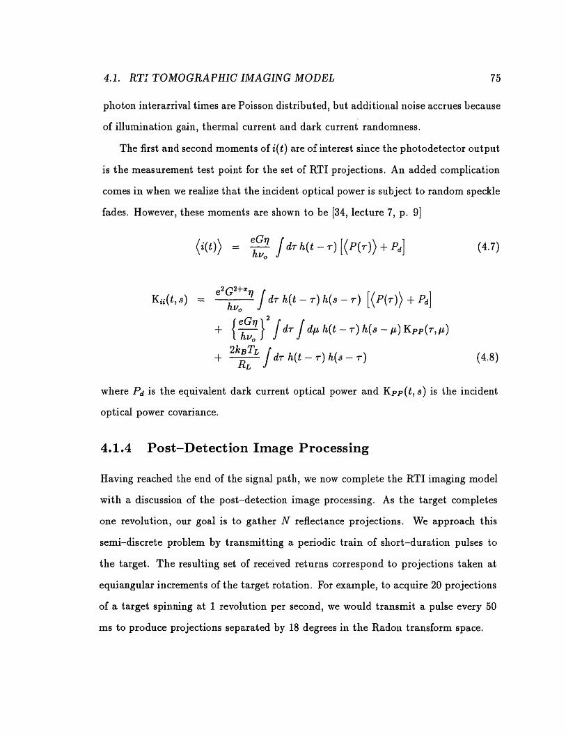
4.1. RTI TOMOGRAPHIC IMAGING MODEL
photon interarrival times are Poisson distributed, but additional noise accrues because
of illumination gain, thermal current and dark current randomness.
The first and second moments of i(t) are of interest since the photodetector output
is the measurement test point for the set of RTI projections. An added complication
comes in when we realize that the incident optical power is subject to random speckle
fades. However, these moments are shown to be [34, lecture 7, p. 9]
(i(t)) he J dr h(t - r) [(P(r)) + Pd] (4.7)
(t, te2G 2+x,Ki(ts) = hv, J dr h(t - r) h(s - r) [(P(r)) + Pd]
+ { eGrhv J d h(t - r)h(s - ) Kpp(r,p)
+ 2k TL dr h(t - r) h(s - r) (4.8)
where Pd is the equivalent dark current optical power and Kpp(t, s) is the incident
optical power covariance.
4.1.4 Post-Detection Image Processing
Having reached the end of the signal path, we now complete the RTI imaging model
with a discussion of the post-detection image processing. As the target completes
one revolution, our goal is to gather N reflectance projections. We approach this
semi-discrete problem by transmitting a periodic train of short-duration pulses to
the target. The resulting set of received returns correspond to projections taken at
equiangular increments of the target rotation. For example, to acquire 20 projections
of a target spinning at 1 revolution per second, we would transmit a pulse every 50
ms to produce projections separated by 18 degrees in the Radon transform space.
75

CHAPTER 4. RTI TOMOGRAPHIC IMAGING PERFORMANCE
Each sample consists of a short duration record of the received signal i(t) after
correcting for the round trip propagation delay to the target center and back. The nth
range projection pe (r) of the target at time t, during the arrival of the illumination
pulse is then defined to be:
Pe.(r) = i(t) (4.9)= 2r/c + t + L/ + 2RT/C
The retarded time terms are calculated to align each projection with the target center
at the range r = 0. The N projections will be subjected to standard tomographic
reconstruction techniques to form a reflectance image of the spherical target. In the
next section we turn our attention to calculating the first and second moments of the
projections pos(r).
4.2 Projection Statistics
In this section we outline the calculations describing the first and second moment
statistics of the projections provided by the above RTI imaging model. We begin by
expressing the mean optical return intensity intercepted by the photodetector as a
function of both the projected target reflectivity and the pulse propagation over the
target surface. After taking into account the photodetection process, this result is
rewritten as the range dependent photodetection mean current. This projection first
moment result exhibits features which begin to hint at some of the image reconstruc-
tion distortion issues. Finally, a similar analysis is performed to determine the second
moments of both the filtered and unfiltered projections used in image reconstruction.
At this point in the discussion, we begin with the derivation of the projection mean
(pon (T)).
In section 4.1.1 we determined that the probe beam Up( p2,t) striking the target
T-plane was a Gaussian beam with a field modulation written in retarded time
76

4.2. PROJECTION STATISTICS
coordinates. In the case of super-range resolution, the short-duration pulse travelling
over the target will freeze the surface motion and leave unresolved any Doppler shift
in the return. Therefore, the return echo UE(fP2, t) at the T-plane will be formulated
by taking the product of probe beam Up(p 2, t) and the projected target reflectance
T(p 2 , t) frozen in place at time t, while retarding the time variable in an appropriate
fashion to account for the round trip delay from the T-plane to the underlying target
surface. This multiplicative model can be constructed by specifying the probe beam
and echo in terms of their time-domain Fourier transforms. Therefore, we model the
return echo at the target as:
UE( 2i,,f) = T(p2, tn) Up(Y2, f) exp {-4rjf [RT - /R - IT22] /c} (4.10)
where Up(Wi2 , f) and UE(P2, f) are the time-domain Fourier transforms of the probe
beam and return echo respectively, and T(pi2, tn) is the target reflectivity evolution
frozen for an instant by the short-duration illumination pulse at time t,. The expo-
nential delay term restores retarded time as the pulse travels from the T-plane to
the spherical target surface and back. Note that Doppler shift has been neglected.
In order to calculate the optical power falling on the photodetector, we must take
the inverse Fourier transform of UE(p2, f) with respect to frequency and then use the
Fraunhofer diffraction formula to propagate the target echo to the laser radar. As in
section 4.1.1, we will assume with insignificant error that the return field modulation
rides a planar wavefront upon arrival at the receiver aperture. This approximation is
valid because the spatial depth of the return field modulation is significantly larger
than the departure of the curving return wavefront from a flat plane. Therefore, the
time retardation from the T-plane to the receiver is L/c, independent of the position
within the aperture.
Using the Fraunhofer diffraction formula, the complete retarded time target echo
77

CHAPTER 4. RTI TOMOGRAPHIC IMAGING PERFORMANCE
caused by the illumination pulse reaching the target at time t, is propagated back to
the laser radar. Taking the expectation of the return field intensity with respect to
the surface roughness and integrating over the receiver aperture results in the mean
optical power (P(t)) falling on the photodetector, giving the following result:
4rka2= 2/ *p(f2+t1)2exp{-|pf+l lb2}P() PT 2 k 2 p 2a L aa 47r2L2 Jd P(i2+,t,) exp 2 /b2}
s(t-tf-Llc-2 [RT- RT- IP2 ]/c) (4.11)
where1
b p2 k2 2 (4.12)
p2 4 2
The derivation assumes that the surface correlation length PT is much smaller than the
target spatial extent aT. The details behind propagating the target surface correlation
structure to the optical field present at the receiver aperture during the course of this
mean power calculation are covered in Appendix B.
This result has elements in common with standard radar equation for the mean
return power from an angle-angle unresolved target [2, §1.2]:
(P) = PTLT x AR X s (4.13)4rL2 47rL2
st~ 2nd1 st 2 3 rd
The first factor is the on-axis target irradiance where GT is the transmitter antenna
gain referenced to an isotropic source. This factor corresponds directly to the RTI
on-axis irradiance term PT/ra in (4.11). The second factor in the radar equation
is the effective reception area of the receiyer aperture. This factor, which accounts
for the portion of the return power collected by the receiver aperture area AR, the
corresponds to the nominal receiver aperture area ra' in the RTI system. The third
factor, cs/41rL2, is the effective target cross-section solid angle subtended from the
78
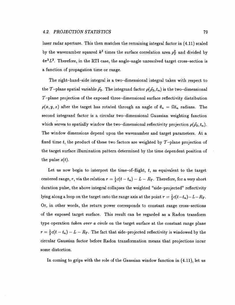
4.2. PROJECTION STATISTICS
laser radar aperture. This then matches the remaining integral factor in (4.11) scaled
by the wavenumber squared k2 times the surface correlation area p and divided by
47r2L2 . Therefore, in the RTI case, the angle-angle unresolved target cross-section is
a function of propagation time or range.
The right-hand-side integral is a two-dimensional integral taken with respect to
the T-plane spatial variable p2. The integrand factor p(p2, t) is the two--dimensional
T-plane projection of the exposed three-dimensional surface reflectivity distribution
p(x, y, z) after the target has rotated through an angle of 0, = Qtn radians. The
second integrand factor is a circular two-dimensional Gaussian weighting function
which serves to spatially window the two-dimensional reflectivity projection p(p2, t).
The window dimensions depend upon the wavenumber and target parameters. At a
fixed time t, the product of these two factors are weighted by T-plane projection of
the target surface illumination pattern determined by the time dependent position of
the pulse s(t).
Let us now begin to interpret the time-of-flight, t, as equivalent to the target
centered range, r, via the relation r = c(t - t) - L - RT. Therefore, for a very short
duration pulse, the above integral collapses the weighted "side-projected" reflectivity
lying along a loop on the target onto the range axis at the point r = 1c(t-t , )-L-RT.
Or, in other words, the return power corresponds to constant range cross-sections
of the exposed target surface. This result can be regarded as a Radon transform
type operation taken over a circle on the target surface at the constant range plane
r = 1c(t - tn) - L - RT. The fact that side-projected reflectivity is windowed by the
circular Gaussian factor before Radon transformation means that projections incur
some distortion.
In coming to grips with the role of the Gaussian window function in (4.11), let us
79

CHAPTER 4. RTI TOMOGRAPHIC IMAGING PERFORMANCE
digress from our discussion and imagine shining a flashlight on a semi-rough surfaced
metal ball. Looking beyond the rear of the flashlight straight towards the ball, we
would see the target illuminated by the flashlight beam. The reflection from the center
of the ball would be the brightest because the normal orientation of the surface would
tend to scatter light directly back to the observer. However, as we move our gaze to
the limb, we would see the scattered light diminish. This occurs because the back
reflection from semi-diffuse surfaces drops as the angle of incidence increases between
the radiation line-of-sight and the surface normal. In the two extreme surface classes
of a Lambertian or highly rough surface and a specular or polished surface, the
back reflection fall-off is either slow or rapid, respectively, as the angle of incidence
increases from zero to 90°. In other words, shiny balls reflect light back from a small
region near the center, while very rough balls apparently reflect light from all over
the illuminated face. Most surfaces behave somewhere in between.
These same effects are modelled by the Gaussian weighting factor above. The
T-plane centered Gaussian window causes the target back reflection to fall-off as
the reflection point moves away from the perceived target center to the limb. The
rate of this fall-off is controlled by the parameter b which is inversely proportional to
the sum of two terms. The first term, k 2 p/RT, models the phenomenon of surface
roughness-aspect angle dependent back reflection. Different surface classes ranging
between specular and Lambertian can be chosen by setting the surface roughness
correlation length PT either as large or small, respectively, in terms of the operating
wavelength A.
The second term, 2/a2, accounts for the finite intensity support that we have
assigned to the target. As the reader will recall from the target modelling discussion,
this parameter was set in place in order to guarantee a closed-form solution after
80

4.2. PROJECTION STATISTICS
Fraunhofer propagation to the receiver. However, this inclusion generates an artifact
in each projection by unnecessarily dimming the target limb. This effect can now be
removed without any loss in accuracy by letting aT grow large and restricting 2 lie
only within the support of the T-plane projection of the target reflectivity.
The received intensity will be directly detected by the RTI laser radar. Using the
previous statistical photodetection model, the mean RTI projection can be written
as:
= y h(t) * (P(t)) [hv0o h~) * t = 2r/c + t, + L/c + 2RT/c
eG7 PT k2p2hv 47raLa L2
J dW2 p(t 2 t,) [ h * s](2r/c+2 /RT -[ 212/c) e-1P212 /b (4.14)
where the symbol * stands for the convolution operator and the origin of the range
coordinate system r has been shifted to the target center. Note that this formula-
tion demonstrates that RTI projections will be smeared by the finite photodetector
response time reinterpreted as the corresponding spatial range depth of the illumina-
tion pulse s(t).
Let us now turn our attention to the projection covariance. As shown in §2.1 of
Appendix B, individual projection measurements will be statistically independent if
N << RT (4.15)PT
which is always the case for meter-sized rough-surfaced targets at infrared or visi-
ble wavelengths. Therefore, the correlation from one projection to the next will be
negligible and the second moment of any consequence will be the projection self-
covariance. Making the same arguments and assumptions as above in the analysis
81

CHAPTER 4. RTI TOMOGRAPHIC IMAGING PERFORMANCE
of the first moment and applying Gaussian moment factoring, §2.1 of Appendix B
demonstrates the projection covariance to be:
1 e2G2+"77 k2a2 PTT p BKpp(rl,r 2) 2 h B( CT) X
4V/i hvo L 2 aL ,p BcT)
2 ) exp -(rl - 2) 47r2 B2 }[{2 2} ]
+ (&G7)2( a) (pt)2 p2 (TCT)2TB x
2 C2T L 471-2~j2C2 (4 .1 6 )(- (r + r2))exp {-(r - 2) 4 } [ { ('(rl + r2) + RT)/ cT} -{ (2(rl + r2))/ cT} ]2+ S/ B 2kTL exP {-(ri- 2) 47r2B2 } (4.16)
where positive values of rl and r2 fall on the far side of the target; the error function,
· (x), is defined to be
(x)- 1 j dt exp{- t2}
and the quantity
B1 - |- (4.17)4r2T2 + B2
is the total system bandwidth. This result was obtained by assuming a Gaussian
shaped pulse s(t) = e-t 2 /T2 with a nominal pulse width of T seconds and a Gaussian
shaped photodetector frequency response h(t) 4 e- f2 /B 2 with a bandwidth of B
Hertz. Furthermore, a low-contrast model for the target reflectivity was adopted,
i.e., p(X, y, ) = p + p(x, y, z) where JSp(x, y, z) << p. This reflectance model was
adopted in order to give closed-form expressions for the spatial integrals over the
target surface during Fraunhofer propagation.
82

4.2. PROJECTION STATISTICS
Note that the covariance is the sum of three terms. The first term accounts for
the effects of photodetector shot-noise driven by the return power, neglecting dark
current and background light. Speckle induced variations within the target return
contribute the second term. The final term is the thermal noise developed across the
photodetector load resistor. The thermal and shot-noise decorrelation distances are
on the order of c/B while the speckle decorrelation distance is proportional to c/B 1.
Likewise, the variance was calculated in Appendix B §2.2 for projections processed
by the inverse Radon transform spatial reconstruction filter If 1. Assuming the rea-
sonable case of useful spatial resolution (i.e., the so-called super-resolution condition
c/B 1 < RT), the filtered projection variance is found to be:
VarPP,(r) ire2G2+"r (kar) PT4 (T) B 3/C2 x
(-r) [ ( + RT) /cT} - {r /cT}]
+ 2 eG77) ka) PTPT p2 (cT) 2 TB3/C2 \hv, L 2 1
(-r)2 [ {( + RT) /cT} - 1{r /cT} ]2
+ 2 R2kBTL 2B (4.18)
This result also assumes the low contrast reflectivity model of the previous result and
identical definitions for s(t) and h(t). Again, the contributions from photodetector
shot-noise, speckle and load resistor thermal noise are summed in that order.
This final variance will be used in the next section along with the projection
mean to formulate a SNR-like figure of merit for filtered backprojection reconstructed
images.
83

CHAPTER 4. RTI TOMOGRAPHIC IMAGING PERFORMANCE
4.3 Reconstructed Image Performance
In this final section we will characterize the performance of the RTI imaging system
in terms of the various forms of aberrations which cause the reconstructed image to
depart from the ideal image. Typically, the analyst will separate aberrations caused
by limitations in the system design from those caused by noise sources corrupting the
measurements. In this analysis, one of our goals is to understand and quantify the
impact of speckle and receiver front-end noise upon system performance by defining
and calculating an image signal-to-noise ratio (SNR). Essentially, this quantity will
compare the squared mean-image to the image variance with respect to both the
shot-, speckle and load resistor noise sources. While this gives an indication of
the noise-induced image fluctuations about the expected image vis-a-vis a fixed
target reflectivity and radar design parameters, the SNR provides little insight into
the deterministic distortions caused by limitations in the system design or imaging
technique. The second goal of this section is to conduct an investigation into this
other class of distortions which will lead to the construction of the imaging system
point spread function (PSF) and ultimately the image resolution. This exercise, which
we now begin, will provide us with a comparative interpretation of the RTI imaging
scenario in relation to the standard two-dimensional tomographic problem.
Cartographers have never produced a undistorted global map of the earth's sur-
face features. Since the RTI imaging system is attempting to produce a flat two-
dimensional image of a three-dimensional surface feature distribution across a sphere,
we suspect that the tomographic reconstruction will build in unavoidable distortions
in addition to the photodetector response smearing indicated earlier. In modeling the
sphere reflectance, T(p), the exposed three-dimensional surface reflectance p(x, y, z)
84

4.3. RECONSTRUCTED IMAGE PERFORMANCE
is projected by parallel rays upon the perpendicular T plane, with the laser radar
observer located at infinity. Cartographers refer to this type of projection as the
orthographic projection (see Figure 4.4(a)) [35]. It is precisely these transverse or-
thographic projections of the reflectance p(x, y, z) on to the T-plane upon which the
RTI Radon transform operates to produce the set of N tomographic projections pe(r).
Any two-dimensional backprojection reconstruction applied to this set of N RTI
projections will form a flat image. Consider the nature of this image. In the standard
tomographic projection of a two-dimensional field, all the points lying on a common
range displacement (scan line) contribute to a single projection ordinate value through
a line integral construction. This same principle holds true for range projections of
rotating three-dimensional targets. The locus of surface scatterers lying in the x-z
plane at a cross-range displacement of r from the target rotation axis will contribute
to the single RTI projection ordinate p(r) through a line integral expression, albeit
a somewhat more complicated formulation which takes into account surface aspect.
If we suppress the z dependence in the three-dimensional problem by choosing a
vantage point above the target north pole, the plane x = r becomes the scan line
x' cos 0 + y'sin 0 = r in the z-axis rotated coordinates. This means that a surface
feature located at the cylindrical coordinates (r, 0, z) within the target frame will be
mapped to the polar coordinates (r, 0) within the image frame by the backprojection--
reconstruction process. Therefore, ignoring the issues connected with formulating
a line integral surface-aspect dependent metric, the reconstructed two-dimensional
image is a projection of the target reflectance p(x, y, z) onto the x-y plane. In other
words, the reconstruction is attempting to reproduce the two-dimensional distribution
ppoi(, y)= p( ,y, +/R - R 2 - y2) + p(,y -R T- - y2). This quantity is
the sum of the northern and southern normal (polar) orthogonal projections across
85

RTI TOMOGRAPHIC IMAGING PERFORMANCE
ProjectionPlane
Parallel
Projection
Lines
/71~
,A/urtnographic Projection of /a Sphere
\ \\\
I7L79Y \
Equator
Normal Projection Transverse Projection
(b) (c)
Figure 4.4: (a) Construction of the Orthographic Projection of a Sphere (b) NormalOrthographic Projection of the Globe (c) Transverse Orthographic Projection of theGlobe
North Pole
./ / / I
7 /7 / / I
1 I I I I
I I
\\\
South Pole
(a)
a.I1 1-4:- r: * _
l--C--C--
Yrt-M-3--'
--�Y -- Fn
I � � \\\\
UH 1 1-4--� 1 ��
U- � � I 1)
I HAV
22.,- I F .F Raetrot 1 - AT a
86 CHAPTER 4.
.Xf i i
I/ IELI I
-_
...'
4�\ \ �
'1, I I \
r
I � \
-- I
I I *-\

4.3. RECONSTRUCTED IMAGE PERFORMANCE
the x-y plane (see Figure 4.4(b)).
The above argument forces us to conclude that the polar coordinates of a surface
feature are preserved through the process of RTI projection formation and backpro-
jection image reconstruction. However, this does not guarantee that the reconstructed
reflectance values of a surface feature will compare equally with the bi-hemispherical
polar target projection. To see how this discrepancy occurs, consider the transverse
orthographic projection of Figure 4.4(c). In any Radon transform of this transverse
projection, the contribution from regions near the equator (e.g. Central America) will
dominate contributions from higher latitudes (e.g. Canada) when compared on the
basis of features with equivalent surface areas on the sphere. The difference between
contributions is explained by a change in surface aspect which causes a foreshortening
effect in the plane of projection. Note that a similar comparison leads to exactly the
opposite conclusion when considering the polar orthogonal projection (Figure 4.4(c)).
These considerations lead us to the preliminary conclusion that the broadside nature
of the RTI projections will emphasize equatorial over limb-sited features in the re-
constructed image.
The above observations indicate that the set of range resolved projections pe(r)
should be rewritten as a Radon transform of the polar projected reflectivity, Ppolar,
before attempting to formulate the imaging system PSF. Beginning with the line
integral description of the T-plane projected reflectivity, this step gives
Po(r)) = h'12P 7aaR 4iL2 J dr' [h * s (2r/c - 2r'/c)
j dx e T I ]/b2 ppoar(X,(x, r'),y (x, I)) (4.19)
Aspect MetricAspect Metric
where the polar projection Ppolar is written in the (x', y') coordinate system rotated 9,n
87

CHAPTER 4. RTI TOMOGRAPHIC IMAGING PERFORMANCE
radians about the z-axis, the surface aspect metric is introduced through the change
of variables from p- to x and z on the target surface and the exponential factor
accounts for the surface roughness-aspect angle effect upon the optical return. We
consider the aspect metric as a two-dimensional function which windows the polar
reflectivity before the line integral transform is performed. Thus, this result is a
generalized Radon transform which weights contributions near the target broadside
(equator) over those from the target limb (polar) regions [27, §II.7]. Furthermore,
the contribution from individual features decreases as the target rotation moves them
away from the y-axis (radar line-of-sight). This behavior accounts for the change ill
surface aspect as target rotation draws features across the illuminated exposure.
This formulation gives us the final link in writing the mean reconstructed RTI
image in terms of the convolution of a two-dimensional PSF with the polar reflectivity
projection ppoir(x, y). The PSF for a specific point (x,, y,) in the (x, y) plane is found
by placing a two-dimensional delta function at (, yo) and calculating the Radon
transform of (4.19) and then computing the convolution of (4.14) to give the set of N
RTI projections. This set of projections is then subjected to filtered backprojection
reconstruction producing the PSF H(x, y, X,, y,). Assuming a Lambertian target for
simplicity's sake, this set of operations gives:
eG7 PT k2 2oH(, y,, y) =T 2 hv, 4ra~ L222
27r N-1 in(C, + SO,) '14 [r cos(O+8o)]2/c2/B( i d y(4.20)__E sin(O. + 0) e - - IB"9 ° '(° " +° il / " o .o (4.20) c0n=O, nE '
[-o,,7r-e] Aspect ReconstructionAngle Projection
Prefiltering
where the dependence upon (O, y) is expressed through the polar coordinates r =
88

4.3. RECONSTRUCTED IMAGE PERFORMANCE
x2 + y2 and tan - l 0o = y,/X,.
Let us take a moment to interpret this formulation. The operator 7H is the inverse
Radon transform projection prefiltering operator F-[If x F(pe(r))]. It is applied to
the detector response time smeared Gaussian projections of the delta function. The
sine function models the projection angle dependent effect of surface aspect change
throughout target rotation. Note that as a feature apparently travels from one target
limb to the other, the corresponding contribution from this sine term goes from zero
to unity on-axis and back down to zero at the far limb. These factors are combined
under the backprojection summation sign to produce an unscaled PSF. This result is
then scaled by various familar laser radar engineering parameters and an additional
factor which depends upon the original position (o, yo) of the delta function. This
last factor accounts for the latitudinal dependence of the surface aspect surrounding
the delta function. Therefore, unlike the formulation developed in chapter 3, the RTI
image PSF is not position independent, and the mean image must now be recovered
through a superposition integral rather than a convolution operation.
The presence of the sine function under the backprojection summation makes a
closed form solution of (4.20) difficult to calculate. However, the normalized PSF has
been numerically calculated and the result is shown in Figure 4.5. The result is a
dumbbell-shaped PSF which is has zero amplitude when located at the origin but
blows-up at the equator. The PSF minor axis lies along the radial axis protruding
from the origin. The major and minor axes lengths of the half-maximum half-
width dumbbell contour are approximately 2.1 and 1.4 times c/B1. Therefore, the
reconstructed RTI image will have finer resolution with respect to the radial axis
than along the transverse radial axis. Thus, we define c/B 1 to be the nominal RTI
resolution.
89

CHAPTER 4. RTI TOMOGRAPHIC IMAGING PERFORMANCE
(t,
Figure 4.5: (a) PSF Reconstruction for N = 144 Projections. (b) PSF Orientation.
Having demonstrated the resolution of the RTI imaging system, we now begin
an investigation of the reconstructed image noise performance via an appropriate
formulation of a signal-to-noise ratio. As in chapter 3, we adopt the following SNR
definition as a measure of reconstruction quality:
(Reconstructed Image Mean at (X,, yo))2
SNR( , yo)var {Reconstructed Image at (, yo)}
On a pointwise basis, this measure contrasts the relative strength of the mean image
to the average strength of noise induced fluctuations.
Retaining our assumptions of a low-contrast reflectivity description and sufficient
system bandwidth to resolve details smaller than the target, the numerator of the
above SNR becomes
6f 2(, YO) IJ dx J dy H(xy, zo0 Yo)SNR(a, o) = (4.21)var {Reconstructed Image at (xo, yo)}
where we have approximated the mean response by taking the product of the slowly
varying low-contrast reflectivity component with the area under PSF. This action is
90
" U
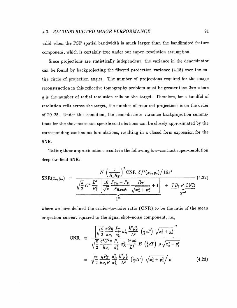
4.3. RECONSTRUCTED IMAGE PERFORMANCE
valid when the PSF spatial bandwidth is much larger than the bandlimited feature
component, which is certainly true under our super-resolution assumption.
Since projections are statistically independent, the variance in the denominator
can be found by backprojecting the filtered projection variance (4.18) over the en-
tire circle of projection angles. The number of projections required for the image
reconstruction in this reflective tomography problem must be greater than 2rrq where
q is the number of radial resolution cells on the target. Therefore, for a handful of
resolution cells across the target, the number of required projections is on the order
of 20-25. Under this condition, the semi-discrete variance backprojection summa-
tions for the shot-noise and speckle contributions can be closely approximated by the
corresponding continuous formulations, resulting in a closed form expression for the
SNR.
Taking these approximations results in the following low-contrast super-resolution
deep far-field SNR:
N B1 RT ) CNR f2(Xo, y)/ 16r5SNR(ox, yo) = (4.22)
G y, B2 16 PTh + PD RT+ - GP +11+ TB1p2 CN
1st
where we have defined the carrier-to-noise ratio (CNR) to be the ratio of the mean
projection current squared to the signal shot-noise component, i.e.,
CNR Ei/ e G PT k PT B cT p
A2 hv a2 R L2 T/P
hv0 a k PT (cT) / 2 +yj (4.23)
91

CHAPTER 4. RTI TOMOGRAPHIC IMAGING PERFORMANCE
and we have normalized by the low-contrast reflectivity component present in the nu-
merator mean response. The above SNR result introduces the thermal-noise equiva-
lent power, PTh, which is the optical power needed to produce a shot-noise component
equivalent to the thermal noise contribution, viz.,
2 kBTL e2 G2+ 77
RL h hv0
and the peak received power, PR,peak
PT 2 ___2
PR,peak iT PT ( cT) pRT
corresponding to a range of r = -RT. This resulting CNR-dependent SNR formula-
tion conveniently expresses performance in terms of physical measures.
From equation (4.22) we see that the filtered backprojection reconstructed RTI
image SNR is directly proportional to the number of projections, N, and the square
of the number or radial resolution cells, q = c/BlRT. The SNR is inversely propor-
tional to the suin of two terms. The first term combines the contributions from the
received power shot-noise, the photodetector dark current shot-noise and the load
resistor thermal noise. This term increases as the point (o, y) is relocated away
from the target boundary toward the image center, eventually dominating the entire
denominator. This condition, which will always occur in a region about the image
center, corresponds to a combined dark current-thermal noise limit. The second de-
nominator term is the excess speckle noise contribution. It is directly proportional
to the CNR and the nominal target reflectivity squared. As the CNR grows with
increasing transmission power, the SNR will grow beyond the dark current-thermal
noise limit in regions away from the image center and eventually saturate at a new
level determined by speckle.
92

4.3. RECONSTRUCTED IMAGE PERFORMANCE 93
Thus, in the high CNR regime, the speckle-limited SNR takes the following value:
8f2(Xo, y) N (c/BRT)2 f2(, y) N (c/BRT) 2 (4.24)p2 167ir2TB 1 p2 4 V'i4
where we have introduced the approximation by equating the transmission pulse
and photodetector response filter bandwidths. Therefore, presuming the absence of
angle-angle resolution, the typical RTI tomographic imaging scenario achieving a
handful of radial resolution cells requires a large number of projections, on the order
of several thousand or more, to drive the SNR up to 5f2(X, yo)/p 2, the conventional
low-contrast speckle-limited laser radar resolved-pixel SNR.

94 CHAPTER 4. RTI TOMOGRAPHIC IMAGING PERFORMANCE

Chapter 5
DTI Tomographic ImagingPerformance
Motivated by the RTI tomography performance analysis, we now turn our atten-
tion to the Doppler-resolved laser radar tomography problem originally outlined in
chapter 1. In this scenario we use a heterodyne laser radar to illuminate a spinning
target to obtain a fixed number of Doppler broadened returns which correspond to
a set of projections of the target reflectance onto the cross-range axis. Tomographic
techniques will then be applied to this semi-discrete Doppler-time-intensity (DTI)
record of the target revolution to reconstruct a two-dimensional reflectance image of
the three-dimensional target. The goal of this inquiry is to examine the performance
of this imaging technique.
Since both the RTI and DTI investigations share the same goals, as well as many
common assumptions and analytical elements, this presentation of the DTI model
and performance analysis is organized in a manner similar to the previous chapter.
Therefore, when appropriate, we will borrow model elements and analytical treat-
ments from the RTI investigation during the DTI presentation. Again, the emphasis
of this chapter is to introduce the reader to the modelling process and the analyt-
95

CHAPTER 5. DTI TOMOGRAPHIC IMAGING PERFORMANCE
ical concepts used to produce the reconstructed DTI image PSF and SNR quality
measures. The companion Appendix C documents the details behind many of the
complicated first and second moment calculations required to obtain these measures.
5.1 DTI Tomographic Imaging Model
In this section we will construct a model of the DTI imaging system. As in the case
of the RTI analysis, model elements and issues will be discussed in the order the are
visited by the energy emitted by the transmitter.
Many features of the monostatic heterodyne laser radar model are shown in Fig-
ure 5.1. We assume the diffuse spherical target is at a constant on-axis position in
the radar's optical far-field at a distance of L meters from the transmitter aperture
and spinning at a rate of Q radians per second.
5.1.1 Transmitter Beam Propagation
In contrast to the RTI scenario, we assume that the DTI imaging system transmit-
ter will interrogate the target with a collimated continuous-wave Gaussian beam of
nominal radius a meters. Therefore, adopting the previous beam specification sans
intensity modulation, the Fraunhofer diffraction formula gives the following scalar
field description for the probe beam Up(p2) perpendicularly striking the T-plane at
the target:
Up(2) = 4 exp jkL + j k 2 exp 2 (5.1)PkP2,- 2 2L 22a (1
Again, the parameter aL = L/kao is the the transmitted beam radius at the target
site.
96

5.1. DTI TOMOGRAPHIC IMAGING MODEL 97
i~ ~ ~ ~ ~ ~~~~9
-4
4)
& {
0 4
g~r
p *S
s ~~ 4)
4)j
-
Figure 5.1:
':·�:· ' ·'· '·:'::·'· ··:;·:··:'··::."····:·:·''"
N

CHAPTER 5. DTI TOMOGRAPHIC IMAGING PERFORMANCE
5.1.2 Target Characterization
The time dependent target reflectivity model presented during the RTI discussion sat-
isfies the requirements for the formulation of a DTI multiplicative reflectivity model.
Therefore, we specify the complex target reflectivity, T, at the point p2 lying in the
T-plane at time t to be:
T( 2 ,t) Vp(f2 ,t) exp{- IP2 2 /4a} exp{jki2 12/RT} exp{2jkh(f 2,t)} (5.2)1st 2nd 3rd 4th
where the four factors take identical roles as in the RTI analysis. Again, we as-
sume that the phase randomness caused by the microscopic surface height random
variable h(p2, t) will cause the received fields to tend toward a circulo-complex Gaus-
sian. Therefore, subscribing to the earlier justifications, we adopt the following phase
statistics:
* (exp{2jkh(5 2,t)}) O
* (exp{2jkh(5 2, t)} exp{2jkh(2', u)}) 0
* (exp{2jkh(i , t)} exp{-2jkh( 2',u)}) 0
I2 - P2' + RT(t - u) 12
As in the RTI case, the same surface roughness issues involving variable surface
aspect, shadowing and multiple reflections are ignored. Since our immediate goal
is a qualitative rather than an exact quantitative understanding, we accept these
approximations.
In contrast to the RTI scenario, we will assume that DTI projections are taken
with sampling dwell times of such length to leave range unresolved. Therefore, in
98
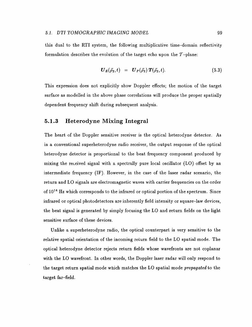
5.1. DTI TOMOGRAPHIC IMAGING MODEL
this dual to the RTI system, the following multiplicative time-domain reflectivity
formulation describes the evolution of the target echo upon the T-plane:
UE( 2,t) = Up(f 2)T(2,t). (5.3)
This expression does not explicitly show Doppler effects; the motion of the target
surface as modelled in the above phase correlations will produce the proper spatially
dependent frequency shift during subsequent analysis.
5.1.3 Heterodyne Mixing Integral
The heart of the Doppler sensitive receiver is the optical heterodyne detector. As
in a conventional superheterodyne radio receiver, the output response of the optical
heterodyne detector is proportional to the beat frequency component produced by
mixing the received signal with a spectrally pure local oscillator (LO) offset by an
intermediate frequency (IF). However, in the case of the laser radar scenario, the
return and LO signals are electromagnetic waves with carrier frequencies on the order
of 1014 Hz which corresponds to the infrared or optical portion of the spectrum. Since
infrared or optical photodetectors are inherently field intensity or square-law devices,
the beat signal is generated by simply focusing the LO and return fields on the light
sensitive surface of these devices.
Unlike a superheterodyne radio, the optical counterpart is very sensitive to the
relative spatial orientation of the incoming return field to the LO spatial mode. The
optical heterodyne detector rejects return fields whose wavefronts are not coplanar
with the LO wavefront. In other words, the Doppler laser radar will only respond to
the target return spatial mode which matches the LO spatial mode propagated to the
target far-field.
99
CHAPTER 5. DTI TOMOGRAPHIC IMAGING PERFORMANCE
In practical heterodyne detectors, great care must be taken to temporally and
spatially tune the LO to match the transmitted field. These systems are designed with
the goal in mind of using relatively inexpensive low frequency electronic components
to accomplish the post-optical detection signal processing. In fact, post-detection
electronic systems often borrow from the same technology used to construct millimeter
and microwave radar IF (10-60 MHz) strips.
Historically, two techniques have been used in practical continuous-wave laser
radar systems to produce frequency shifted LO beams. First, the transmitted optical
beam is sampled and fed through an acoustic-optic (AO) modulator driven by the
IF oscillator. The LO output beam shares the same spatial mode as the transmission
beam while experiencing an optical carrier frequency shift equal to the IF. The second
approach uses a separate LO laser cavity whose length is adjusted using a piezo-
electric (PE) device to produce the desired IF shift. The output beat signal from a
second heterodyne detector which samples both the LO and the transmission beam is
compared with an IF reference to generate the error signal controlling the PE crystal
drive voltage.
In developing a mathematical model of the optical heterodyne detector, one finds
that the beat frequency term is proportional to the square-root of the LO power,
AThio. Therefore, laser radar systems are operated with LO powers as high as possible
to maximize return signal sensitivity and minimize background light response. In
this mode of operation, the photodetector LO shot-noise component dominates the
contributions from both the return signal and background light shot-noise and the
detector load resistor thermal noise. Under these assumptions, we now introduce a
theoretical model of optical heterodyne reception which assumes perfect LO wavefront
matching with the return. As with the previous optical field work, we continue to
100

5.1. DTI TOMO GRAPHIC IMAGING MODEL
express signal envelopes in terms of complex quantities.
In the high local oscillator power (PLO) regime, the response of the IF heterodyne
det -tor can be modeled as [9, 10]
r(t) = Re [r(t) exp{27rjvIFt}] (5.4)
where r(t) represents the complex envelope of the received signal. This envelope
can be broken down into two components and written in the form r(t) = y(t) + n(t)
where
y(t) =/ dp Ur(p3, t) jLo(i3 ,t) (5.5)
is the PLO normalized heterodyne return signal. The return y(t) is expressed as a
heterodyne mixing integral of the product of the optical return U,(fi 3, t) and the local
oscillator field VP/Lo Lo( 3). These fields are spatially integrated with respect to the
position vector pi3 lying on the photodetector (PD) surface.
The second term n(t) is a circulo-complex white Gaussian noise process with the
following statistics:
* (n(t)) = 0
* (n(t) n*(u)) =- 8(t - u).
The parameter 77 is the photodetector's quantum eft;riency and h is Planck's constant.
This noise term is the normalized local-oscillator shot-noise at the receiver front-end.
The shot-noise contributions from the received optical return and background light
are neglected in lieu of the dominant local oscillator field.
Traditionally, the analyst would propagate the return echo UE(f2, 1t) = U(P2)'
T( 2, t), back from the target through the receiver aperture to the photodetector
101

ChAPTER 5. DTI TOMOGRAPHIC IMAGING PERFORMANCE
surface (PD) in order to evaluate the heterodyne mixing integral. However, the an-
tenna theorem [36] states that (5.5) maybe evaluated by integrating the product
of the return echo UE(p2,t) at the T plane with the local oscillator spatial mode
Lo(ia3) propagnated to the T plane. This back propagation is understood to take
place in the sense that he LO spatial mode also travels through free-space along-
side the transmitter beam to the target. If we assume the local oscillator spatial
mode is matched to the transmitter spatial mode at the transmitter/receiver aperture
(that is, Lo(1') = T(Pl)), then the back propagated local oscillator field becomeF
v/Lot p(2) at the plane T and the mixing integral is then
y(t ) = PT J d 2 , (p2) T( 2, t). (5.6)
This description of heterodyne reception will used as a starting point for the projection
moment calculations in the next section.
5.1.4 Post-Detection Image Processing
Having reached the end of the signal path, we now complete the DTI imaging model
with a discussion of the post-detection image processing. The details of projection
extraction from the received signal are shown in Figure 5.2.
As the target completes one revolution, our goal is to gather N reflectance projec-
tions. We approach this semi-discrete problem by sampling the received heterodyne
output signal r(t) at regular time intervals. The set of sampling instants correspond
to equiangulr increments of the target rotation.
Each sample consists of a short duration record of the received signal r(t). The
nth record is formed by multiplying the received signal by a window centered on the
sampling instant tn = 0,l/n where in, is the angle of the nth projection psn(v). To ease
the mathematical analysis in the next section where we take projection moments, we
102

5.1. DTI TOMOGRAPHIC IMAGING MODEL 103
0
0L1
0
0
cn
0!' PI ..
(UQ0
0C.)
o~~~~~~
o C)C) r'
C)C
.1 .i.
Figure 5.2:

CHAPTER 5. DTI TOMOGRAPHIC IMAGING PERFORMANCE
have chosen a Gaussian profiled time window. The parameter T is the projection
observation dwell time.
Each projection pen(v) is then formed by computing the magnitude-squared fre-
quency spectrum of the associated signal record. This results in projections which
are proportional to the Doppler return spectrum of the rotating target. Finally, the
projection independent variable v (Hz) is transformed into the cross-range variable
r by the Doppler relation = 2rQ/A. Thus, the set of projections is a train of the
magnitude-squared Fourier transforms of the Gaussian time windowed signal r(t).
The N projections will be subjected to standard tomographic reconstruction tech-
niques to form a reflectance image of the spherical target. In the next section we
turn our attention to calculating the first and second moments of the projections
ps(v) ji=2r0/A
5.2 Projection Statistics
In this section we outline the calculations describing the first and second moment
statistics of the projections provided by the above DTI imaging model. An investiga-
tion into the time dependent heterodyne return correlation reveals a separable struc-
ture, which is exploited in formulating the heterodyne return power spectrum and
deriving the projection mean. The resulting projection first moment clearly demon-
strates the interplay between dwell time duration and spatial resolution and begins
to hint at some of the image distortion issues involved in reconstruction. Finally, a
similar analysis is performed to determine the second moments of both filtered and
unfiltered projections. At this point in the discussion, we begin with the derivation
of the projection mean (po(v)).
104

5.2. PROJECTION STATISTICS
Referring to Figure 5.2 we see that the projection mean can be written as
(Pe ( ))
(L(v) L(v)) (5.7)
= J du (- )r(u) e-27rJv(u-tn) e- 4(u-t )2/T2 x
JO dv ( 2) r(v) e2jv(v-tn) -4(v-t.)2/T2
- j_ du _ dv (y(u) y*(v)) e- 2 ij v(u-v) ( 8 ) e-4((u-tn)2 +(vt) 2)/T2 +
J do J o no) n -21i,(U-U) 8 2 -4((.-tn)2+(V-tn )2 )IT2du dv (n(u) WM) e e
(5.8)
Pn ((v)), (P± n ())n (5 9)
where we have used the statistical independence of the return y(t) and the noise n(t).
The second double-integral in (5.8) is the local oscillator shot noise contribution to the
projection mean. Recalling that we have normalized by the local oscillator power,
a straightforward calculation reveals this contribution to be hvo/1. This constant
value provides no information about the target, and therefore, will be neglected in
our theoretical analysis. However, in actual image reconstruction systems, the effect
of this bias can be removed by subtracting hvo/I from each projection. It is the first
double-integral that formulates the target return component of the projection mean.
The challenge is to evaluate and interpret this double-integral involving (y (u)y*(v)).
Substituting equation (5.6), the heterodyne return component, this inner expec-
tation can be written as
(y(u)y*(v))= Jd 2 JdP 2 'PT (5 2) [d( 2')]2 (T(,u)T( 2 vt)) (5.10)
105

CHAPTER 5. DTI TOMOGRAPHIC IMAGING PERFORMANCE
where the expectation is taken over the random microscopic surface fluctuations of
the sphere.
Before evaluating the above covariance, let us consider the relationship between
the different physical processes which give rise to the return signal y(t). Intuitively,
the statistical behavior of this signal can be broken down into two largely independent
factors which correspond to physical processes which take place over relatively short-
and long-term time scales, respectively. This separation is natural when one realizes
that return variations, rising from the passing of speckle lobes over the receiver aper-
ture, have nearly stationary statistics over time scales in which there is little apparent
motion of the surface reflectivity distribution over the target. In other words, under
super-Doppler resolution conditions in which the dwell time T is chosen sufficiently
small to render negligible surface feature motion over the expose face of the target,
the heterodyne signal statistics are stationary during the dwell time, with first and
second moments which depend upon the target aspect or projection angle. Therefore,
on the longer time scale stretching over an inter-projection sampling period, we would
expect each average DTI projection to match with some type of Radon transform of
the target reflectivity taken at an aspect corresponding to the projection angle.
This approach is formalized by applying the Schell approximation to the hetero-
dyne component covariance formulation [40]:
(y(u)y*(v)) K ((u + v),u-v) var ((u + v)) k(u-v)
where the speckle decorrelation modelled by k(u - v) falls off much more quickly than
(ly(½(u + v))l2) _ var ((u + v)) which accounts for the return fluctuations caused
by the motion of the reflectivity distribution.
For the sake of convenience, we separate the short- and long-term time scales by
adopting the following sum and difference time coordinates according to our standard
106

5.2. PROJECTION STATISTICS
pattern
u = t + /2
v = t- r/2
where the time coordinate t, now accounts for long-term projection evolution while r
describes short-term speckle return variations. Defining the return power spectrum
to be the Fourier transform of the Schell approximation with respect to the small
time scale changes, r, we have, at time t,:
S(tn, f)
= j dr (y(t, + ) *(tn1 - -2
PTk 2 a x ra X 147rL2 0 4wL2
1k i± (p. I f, p) tn) exp {- (p +( ( f)2)b2} (5.11)
Two-DimensionalGaussian Window Function
where we have defined
b2 = (5.12)2 T
- + 2RT
The missing details behind the derivation of the above result are supplied in §1 and §2
of Appendix C. As in the RTI case, this result assumes the assumptions of spotlight
mode target illumination, RT < L and PT << aT.
Recalling the RTI mean projection discussion, the right-hand-side of the above
result is written in the standard radar equation formulation where the first factor is the
on-axis target irradiance, the second is the effective aperture area of the monostatic
heterodyne receiver and the third factor is the Doppler frequency f resolved target
cross-section divided by 4rL 2. The integral component is single-dimensional and
107
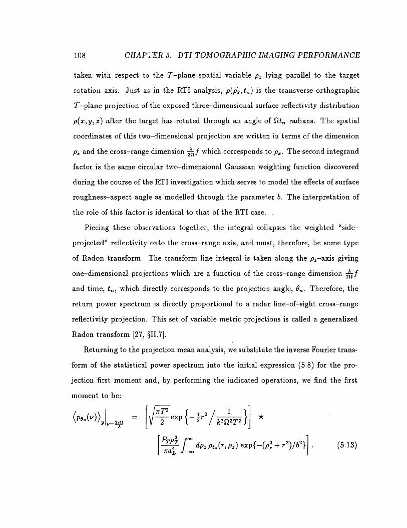
CHAP'"ER 5. DTI TOMOGRAPHIC IMAGING PERFORMANCE
taken with respect to the T-plane spatial variable pz lying parallel to the target
rotation axis. Just as in the RTI analysis, p(,p2, t,) is the transverse orthographic
T-plane projection of the exposed three-dimensional surface reflectivity distribution
p(x, y, z) after the target has rotated through an angle of Qtn radians. The spatial
coordinates of this two-dimensional projection are written in terms of the dimension
pz and the cross-range dimension jf which corresponds to pa. The second integrand
factor is the same circular two-dimensional Gaussian weighting function discovered
during the course of the RTI investigation which serves to model the effects of surface
roughness-aspect angle as'modelled through the parameter b. The interpretation of
the role of this factor is identical to that of the RTI case.
Piecing these observations together, the integral collapses the weighted "side-
projected" reflectivity onto the cross-range axis, and must, therefore, be some type
of Radon transform. The transform line integral is taken along the pz-axis giving
one-dimensional projections which are a function of the cross-range dimension N f
and time, t,, which directly corresponds to the projection angle, 0,. Therefore, the
return power spectrum is directly proportional to a radar line-of-sight cross-range
reflectivity projection. This set of variable metric projections is called a generalized
Radon transform [27, §II.7].
Returning to the projection mean analysis, we substitute the inverse Fourier trans-
form of the statistical power spectrum into the initial expression (5.8) for the pro-
jection first moment and, by performing the indicated operations, we find the first
moment to be:
=IV [ { 2/ exp }]
[ 4 f dp p(r,pz) exp{-(p2 + r2)/b2}] (5.13)1 TYT0_,27twaL I"J-o X~')ja.~ (5.13)7r4f0 Z x
108

5.2. PROJECTION STATISTICS
This result assumes that the exposed distribution of the target reflectivity suffers from
little apparent motion during the observation dwell time. Note the we have expressed
the mean as a convolution of two functions with respect to the cross-range variable
r. The first function is a one-dimensional Gaussian form whose width is inversely
proportional to the product of the laser wavenumber k, the target rotation rate Q2 and
the observation dwell time T. The second function is the generalized Radon transform
of the projected reflectivity as formulated within the power spectrum expression.
(The reflectivity subscript t, denotes the projection's time dependence.) Recalling
the flashlight-ball gedanken experiment, this is a cross-range projection of a "net"
reflectivity distribution which takes into account the joint issues of aspect and surface
roughness. The convolution then smears this projecticn with an instrument function
whose spatial resolution is inversely proportional to the observation dwell time. It
is the width of this instrument function which will ultimately determine the final
resolution of the reconstructed image.
Let us turn our attention now to the projection covariance. As mentioned pre-
viously, the receiver aperture speckle coherence time is a fraction of the observation
dwell time. Therefore, the correlation from one projection to the next will be negligi-
ble and the second moment of any consequence will be the projection self-covariance.
Making the same arguments and assumptions as above in the analysis of the first
moment and applying Gaussian moment factoring, §3 of Appendix C demonstrates
the projection covariance to be:
[hvc WT2 PTp2b 2 1 (r + r)2 Kpp(ri,r2 ) [ + P-T- pexp 7 exp {-( - ) / 2 (514)
109

CHAPTER 5. DTI TOMOGRAPHIC IMAGING PERFORMANCE
where
b2 12 (5.15)
2 k 2 Q22T2 '
This result was obtained by assuming a low contrast model for the target reflectivity,
i.e., p(x, y, z) = p+ p(x, y, z) where 16p(x, y, z)j << p. This simplification was adopted
in order to give closed-form expressions for the spatial integrals over the target surface
during Fraunhofer propagation.
Note that this result is the product of two factors. The first factor is the square of
the sum of two terms. The first term hvo/7 accounts for the LO shot-noise contribu-
tion to the projection covariance while the second term adds in the target's speckle
contribution. The non-negligible support of this last term is equal to the parameter
a, the radar resolved target extent. This implies that r2 is proportional in some man-
ner to the unresolved target cross-section. The second factor in the above product
is written as a function of the spatial coordinate difference, r - r 2. Therefore, the
projection decorrelation length is equal to V'2/kQT.
The variance for projections processed by the inverse Radon transform reconstruc-
tion filter H(f) = If I is also calculated in Appendix C §2. Assuming the reasonable
case of useful spatial resolution (i.e., the super-resolution condition l/kQT < A), the
filtered projection variance is found to be:
2k2 Q2T2 hv + rT , PTp2b2 1 (rl + r2) 2
varp,(r) 87r2 v 2 kTP P 2 42 (5.16)8-2 77 2a kTo- 2 4or
This result also assumes the low contrast reflectivity model of the previous result.
As in the RTI analysis, the first and second moments will be used in the next
section to formulate a SNR-like figure of merit for reconstructed images.
110

5.3. RECONSTRUCTED IMAGE PERFORMANCE 111
5.3 Reconstructed Image Performance
In this final section, as in the case of the RTI analysis, we will find it convenient to
characterize the reconstructed image distortion performance in terms of a PSF and
the image noise performance in terms of a SNR.
In defining an appropriate PSF, we must deal with the same issues encountered
during the RTI discussion in working with the T-plane transverse orthographic pro-
jections of the target reflectance in the course of taking Radon transforms. Therefore,
the set of Doppler resolved projections pe(r) should be rewritten as a Radon trans-
form of the polar projected reflectivity, Ppolar, before attempting to formulate the
imaging system PSF. This action places both the RTI and DTI PSF analysis on a
common basis, which will then allow direct performance comparisons. Beginning with
the line integral description of the T plane projected reflectivity, this step gives the
mean as
P r)/ praT , exp-r2 2( (4 2 k2Q2T2
/°dy - eT[R -2]/ b p (X (r, y), y (r, )) (5.17)
Aspect Metric
where the polar projection Ppolar is written in the (', y') coordinate system rotated 0Bn
radians about the z-axis, the surface aspect metric is introduced through the change
of variables from p, to y on the target surface and the exponential factor accounts for
the surface roughness-aspect angle effect upon the optical return. Thus, this integral
is a generalized Radon transform which weights contributions near the equator over
those from the polar regions.
This formulation gives us the means to write the average reconstructed DTI image
in terms of the convolution of the PSF with the polar reflectivity projection. Applying
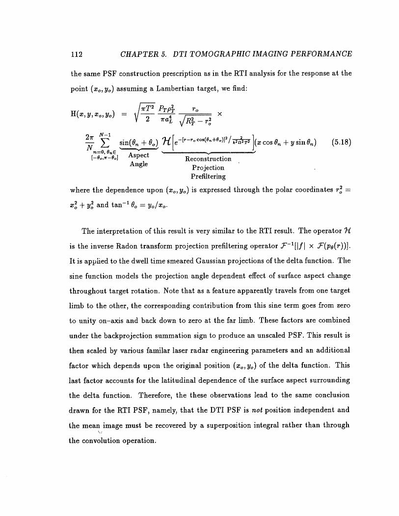
CHAPTER 5. DTI TOMOGRAPHIC IMAGING PERFORMANCE
the same PSF construction prescription as in the RTI analysis for the response at the
point (xo, y) assuming a Lambertian target, we find:
rT2 PTP42 roH(x, y, Z0,Yo) 4 2 T -r X
2 N sin(O + o) -[ -[r-r +'/ (cossno 2n2 2 ( C + y ill .) (5.18)Nn=o, oE "-[-0o,7r-8] Aspect Reconstruction
Angle ProjectionPrefiltering
where the dependence upon (xO, yo) is expressed through the polar coordinates r =
x2 + y2 and tan -1 6o = yo/x 0 .
The interpretation of this result is very similar to the RTI result. The operator 7
is the inverse Radon transform projection prefiltering operator F-[If I x (ps(r))].
It is applied to the dwell time smeared Gaussian projections of the delta function. The
sine function models the projection angle dependent effect of surface aspect change
throughout target rotation. Note that as a feature apparently travels from one target
limb to the other, the corresponding contribution from this sine term goes from zero
to unity on-axis and back down to zero at the far limb. These factors are combined
under the backprojection summation sign to produce an unscaled PSF. This result is
then scaled by various familar laser radar engineering parameters and an additional
factor which depends upon the original position ( 0 , yO) of the delta function. This
last factor accounts for the latitudinal dependence of the surface aspect surrounding
the delta function. Therefore, the these observations lead to the same conclusion
drawn for the RTI PSF, namely, that the DTI PSF is not position independent and
the mean image must be recovered by a superposition integral rather than through
the convolution operation.
112

5.3. RECONSTRUCTED IMAGE PERFORMANCE
Figure 5.3: (a) PSF Reconstruction for N = 144 Projections. (b) PSF Orientation.
The presence of the sine function under the backprojection summation makes a
closed form solution of (5.18) difficult to calculate. However, the normalized PSF has
been numerically calculated and the result is shown in Figure 5.3. The result is a
dumbbell-shaped PSF which is has zero amplitude when located at the origin but
blows-up at the equator. The PSF major axis lies along the radial axis protruding
from the origin. The major and minor axes lengths of the half-maximum half-
width dumbbell contour are approximately 1.5 and 1.0 times 1/kQT. Therefore,
the reconstructed DTI image will have finer resolution with respect to the transverse
radial axis than along the radial axis. Thus, we define 1/kf2T to be the nominal DTI
resolution.
Having demonstrated the resolution of the DTI imaging system, we now begin
an investigation of the reconstructed image noise performance via an appropriate
formulation of a signal-to-noise ratio. As in the previous chapter, we adopt the same
113
, ., \

CHAPTER 5. DTI TOMOGRAPHIC IMAGING PERFORMANCE
SNR definition as a measure of reconstruction quality:
f 2 (o, yo.,) d d y H(x, y, xo,, y)SNR(o, yo) = (5.19)SNR(x, y) var {Reconstructed Image at (,, y,)}
On a pointwise basis, this measure contrasts the relative strength of the mean image
to the average strength of noise induced fluctuations for a low-contrast target under
super-resolution conditions which adequately resolve the bandlimited surface feature
distribution 6f(x,, y).
As demonstrated in Appendix C §3, projections are statistically independent, the
variance in the numerator can be found by backprojecting the filtered projection
variance (5.16) over the entire circle of projection angles. As in the RTI case, for a
handful of resolution cells across the target, the number of required projections is on
the order of 20-25. Under this condition, the semi-discrete variance backprojection
summations for the shot-noise cross speckle and the speckle cross speckle contri-
butions can be closely approximated by a factor proportional to Ne - ' /2 2Io(ro/2 r2)
and Ne -' o / 2 Io(ro/ 2), respectively, resulting in a closed form expression for the SNR,
where Io is the zeroth order modified Bessel function.
Taking these approximations results in the following low-contrast super-resolution
SNR:
SNR(xo,y,) =
8f 2(xo, yo) N (kT - CNR cos2bp/16 3
e_ 2-/CNB + 2 3r/4 2 Io(rI /4u2) + p2CNR e-r2/2 Io(ro/2 2
1 st 2nd 3rd
where we have defined the carrier-to-noise ratio (CNR) to be the ratio of the mean
114

5.3. RECONSTRUCTED IMAGE PERFORMANCE
projection to the LO shot-noise spectrum, i.e.,
CNR I (p(rp))(hv/77)
= PTp b2 r/2r2 (5.21)
2 hv,o a koe
where we have normalized by the low-contrast reflectivity component present in the
CNR numerator mean response. In the above SNR formulation we have assigned
as the equivalent target latitude of the point (xo, yo). This resulting CNR dependent
SNR formulation conveniently expresses performance in terms of physical measures.
Thus, the filtered backprojection reconstructed DTI image SNR is directly propor-
tional to the number of projections, N, the square of the number of radial resolution
cells, q = b2 /kQTo- and the cosine squared of the latitude 0b. The SNR is inversely
proportional to the sum of three terms, the shot-noise x shot-noise, the shot-noise
x speckle and the speckle x speckle in that order. As the CNR grows with increasing
transmission power, the SNR will grow beyond the shot-noise limit imposed by the
first two denominator terms and eventually saturate at a new level determined by
speckle.
Thus, in the high CNR regime, the speckle-limited SNR takes the following value:
f 2 (X0' yo) N (k -) CNR cos2 167r3
p2CNR e-'/2 2 Io(r/2o2)
This speckle limit rises from a value of zero at the reconstructed image center to
a peak value at the image boundary. As in the RTI case, presuming the absence of
angle-angle resolution, the typical DTI imaging scenario achieving a handful of radial
resolution cells across a Lambertian target requires a large number of projections, on
the order of several thousand, to drive the SNR up to 8f 2(Xo, yo)/p 2, the conventional
low-contrast speckle-limited laser radar resolved-pixel SNR.
115

116 CHAPTER 5. DTI TOMOGRAPHIC IMAGING PERFORMANCE

Chapter 6
Comparison with ExperimentalResults
This chapter discusses a comparison between the theoretical PSF performance pre-
dictions of the past two chapters and the RTI and DTI work performed at the Laser
Radar Measurements group at the M.I.T. Lincoln Laboratory.
Researchers at this facility have noted that reconstructed RTI images tend to
emphasize target boundaries, leaving interior regions unresolved, while DTI images
take on a target silhouette-like appearance where, to the contrary, boundaries have
been de-emphasized and smoothed [37]. Kulkarni, et al, investigated these effects by
reconstructing simulated RTI and DTI images of a cylindrical target rotating about
the major axis (z-axis). Their results, reproduced in Figure 6.1, are RTI ((a), (c))
and DTI ((b), (c)) images for both a Lambertian surface ((a), (b)) and a second
surface ((c), (d)) which only exhibits strong reflectance a grazing angles of incidence
(i.e., their "non-physical BRDF" target). These figures plainly show for Lambertian
surfaces that indeed RTI resolves target outlines while DTI produces smoothed target
silhouettes.
Even though our analysis used a number of approximations during the devel-
117

COMPARISON WITH EXPERIMENTAL RESULTS
AIISN31NI tV3N1 3AI138
I
w-J
-a-
wacc
z <
w -W LL a
0U.
a
Figure 6.1: Comparison of RTI and DTI Reconstructions
r I __
I f i .... ...
CHAPTER 6.118
----.... 1. -

119
opment of the RTI and DTI results, the above patterns can now be qualitatively
explained in light of the analysis of the previous two chapters. For the case of RTI,
the trans-radial orientation of the dumbbell-shaped PSF means that details along
the radial axis will be resolved. Therefore, RTI imaging will highlight the target
outline. On the other hand, the radial orientation of the similarly dumbbell-shaped
DTI PSF will tend to smear radial details. Therefore, DTI imaging will soften the
projected target boundary and fill the reconstruction interior. In our imaging model,
if we assume that a non-negligible uniform reflectance confined to an equatorial belt
about the spherical target approximates the simulated cylindrical target in [37], then
on a qualitative basis, the above RTI and DTI reconstruction behavior is confirmed
by the results of Figure 6.1.
Note that RTI and DTI performance is reverEsd for the "non-physical" target.
Again, this dual behavior is predicted by our PSF formulations. The strong return a
grazing angles of incidence corresponds to responses taken along the trans-radial axis
of the RTI and DTI PSF's. At these orientations, the RTI and DTI PSF's are respec-
tively, relatively wide and narrow. Therefore, we would expect the DTI reconstruction
to resolve the target boundary while the RTI image would approximate a silhouette.
Again, this prediction is supported qualitatively by the simulated reconstructions in
Figure 6.1.

120 CHAPTER 6. COMPARISON WITH EXPERIMENTAL RESULTS
Chapter 7
Conclusions
This dissertation analyzes the statistical performance of both direct-detection RTI
and heterodyne detection DTI tomographic laser radar imaging systems in the pres-
ence of speckle and photodetector shot-noise. This was accomplished by construct-
ing dual mathematical models for each system when interrogating a rotating diffuse
spherical target sited in the radar's optical far-field, and then calculating first and
second projection moments. These moments where used to develop two measures
of reconstructed image quality: the point-spread-function (PSF) and the pointwise
signal-to-noise ratio (SNR), which characterized distortion and noise performance,
respectively.
The resolution capabilities of both RTI and DTI are indicated by the contours of
their associated PSF's. In each case, the dumbbell-shaped PSF response peaked on
the equator of the spherical target and then fell to zero at the poles. This behavior is
readily explained by the effect of surface foreshortening as one moves from the equator
toward either pole. The nominal half-height half-width resolution cell size is oil the
order of c/B 1 and 1/kfT for RTI and DTI, respectively. The cross orientation of
the RTI and DTI PSF's predicts that range-resolved imaging will reconstruct target
boundaries while Doppler-resolved imaging will produce smoothed target silhouettes.
121
CHAPTER 7. CONCLUSIONS
These predictions are in agreement with the simulations performed by others.
The noise performance of both RTI and DTI systems was written in terms of a
carrier-to-noise (CNR) formulation of the reconstructed image SNR. In each case the
CNR was conveniently defined as a measurable physical quantity which entailed many
of the model parameters. For RTI, performance was limited at low transmission power
levels by presence of photodetector thermal noise and dark current. Local-oscillator
shot-noise limited DTI SNR performance at low transmission levels. However, in the
high transmitter power regime, radially dependent speckle SNR limits were identified
for both RTI and DTI. In both cases, this speckle limit was found to be directly
proportional to the number of projections and inversely proportional to the square
of the number of radial resolution cells across the target. Therefore, in the speckle
limit, these imaging techniques incoherently average speckle noise via tomographic
backprojection reconstruction while retaining all of the inherent resolution capabilities
of their underlying range- or cross-range-resolving systems. However, in scenarios
achieving a handful of radial resolution cells with a modest number of projections,
the SNR performance of both imaging systems was found to be below both unity and
the conventional low-contrast speckle-limited laser radar resolved-pixel SNR.
Beyond the results presented here, this work may be an appropriate foundation
for proceeding with a more general analysis. As implied during the error analysis at
the end of chapter 3, a projection gathering system in which the target reflectance
is regarded as a deterministic function could be modelled by attempting to meld the
distortion and noise issues by adopting a mean-squared-error (MSE). This quantity
would sum an image bias term, a measure of the departure lf the system PSF from the
ideal two-dimensional delta function PSF, and a second variance term which would
account for the reconstruction noise strength. We could then imagine generalizing this
122

123
model by relaxing the deterministic restriction on the target reflectance and assuming
an appropriate random model. In this case, one could compute the MSE over the
reflectance ensemble by taking conditional expectations of the bias and variance terms
and then minimize this quantity over the system filters to produce an minimum error
imaging system design. Finally, one could approach the problem by developing a more
general model which removes the tomographic reconstruction assumption to allow
optimization over all possible image reconstruction algorithms and target observation
strategies.

124 CHAPTER 7. CONCLUSIONS
Appendix A
This appendix presents the details of the projection cross-correlation calculation dis-
cussed in §3.2 for the case of unequal projection angles (i.e., 01 02). Beginning with
equation (3.9) we have
(R(rl, O)R*(r2 , ))
~00 coe 2jk(R+, y)= 9j J dx1dy's(x I (x, '1), yl(x', y))b,(x'l, Yl )e(O f oo00
J I dx2dY2s (X2(X2,y2), Y2(x ,y2))b,(x',y)e - 2 2( n+ y ) (3.9), (A.1)_00 00
=--j dmldy'f(xl(xl Y'), Y(X' Y'))
exp (2jAkyl) exp (-2jk[-x' sin(L - 02) + Y1 cos(0- 02)])
1 J(x~ -rl)2) ((x cos(9i-2) + ysin(l-2)-r2) 2exp exp- 2r )
(A.2)
where the cross-correlation is now written in terms of the (xi, y') Cartesian coordinate
system (cf. Figure 3.2 and Figure A.1). Suppose that in the (x, y4) coordinate system
the scan lines (rl, 90) and (r2, 2) intersect at the point denoted as (' , y). Solving
for these coordinates,
XX = rT
YX = r 2 SC( 1 - 2) - r1cot(9l - 2)-
125

APPENDIX A.
Footprint
itersection
oint (, y~)
Scan Line
(r, ,0 1)
Figure A.1: Placement of the (x, y), (xi,y"), (xIy"), and (x.',y') Coordinate Sys-tems with respect to the Scan Lines.
126
127
We now choose a new Cartesian coordinate system (, y1') whose axes are parallel to
the (x, y') coordinate frame and whose origin lies on the scan line intersection point
(x, Yx ). This axis translation is thus
II I Ixl = x1 - x
Y1 = Y1 - Yx
Expressing the cross-correlation in terms of this new coordinate system:
(R(ri, )R (r2, ))oo r00oo
d1cd,'f2( + Y1 + X) Y1l( +X xY + ))00 x0
exp (2jk(y' + y )) exp (-2jk[-(Z + x) sin(01 - 02) ( +' cos(01-- 02)])
r2 exp (- (z;)2/r) exp (- ( cos(01 - 02) + y' sin(01- 02))2/r) . (A.3)
Note the simplified the Gaussian forms. Finally, we rotate the (x', y"') coordinate axes
through an angle of AO/2 = -(V1 - 02)/2 to form the (x'1, y.") Cartesian coordinate
frame. The origin of (x', y") lies on the intersection point (x, yx ); the y"' axis bisects
the two scan lines (ri, 08) and (r2 , 02) at the (x' ,y) intersection point. Rewriting
the formulation of the cross-correlation in this final coordinate system, we have
(R(ri, O)R(r2, 6))
= J~0j dlx'' dy'": :1 1
f(('(x",Y 1") + , ''Y1 XIY) + '), yl(X (,") +'I '1 (X '"yj") + ')I Iexp (2jk(yl'(x, Y1) + Yx))
exp (-2jk[-(x(l',Y111) + in(01 -02) + (Y1(, Y ) + Y ) cos(,0 - 02)])
2 [I sin(01 -02)1 (_ (xII92 ( (y~I)22 Is(0 2)1- "exp I (y M) " y 2"
si(e -2)1 7 rr exp r/ cos2 (AO/2) r / sin2 (A0/2) '(A.4)

APPENDIX A.
Note that the term in brackets on the last line is a two-dimensional Gaussian prob-
ability density function (PDF) form centered on the intersection point with major
and minor axes lengths which vary with the angle of attack 92 - 81. The argument
of f(., ) within the original (x, y) Cartesian coordinate system defined in Figure 3.2
is simply the point (, y9). The rest of the integrand is a complex phase factor.
Therefore, asserting the same argument in passing to the Radon transform, if r be-
comes small enough such that f is smooth under the significant part of the Gaussian
PDF footprint, then the cross-correlation may be approximated by
(R(rl, O)R"(r2, 0)) - -sin( - 2) f( ) (A.5)
which in magnitude squared becomes
(R(ri, )R* (r2, 9))1 = sin2 4( - 92) f 2(zX,yO). (A.6)sin 2(01 0 2)
128

Appendix B
Thlis appendix details the assumptions and approximations behind the development
of the RTI mean projection optical power (4.11) and both the RTI projection vari-
ance (4.18) and covariance (4.16) for filtered and unfiltered projections, respectively,
produced by a Gaussian illumination pulse originating from a radar sited in the tar-
get deep far-field and reflecting from a low-contrast surface. These calculations also
provide a convenient framework for demonstrating inter-projection statistical inde-
pendence under typical RTI imaging scenarios. The essence of these derivations is the
determination of the return optical field covariance by propagating the target surface
covariance via the Fraunhofer diffraction formula.
B.1 RTI Mean Projection Formulation
In this section we compute the time dependent optical power falling on the receiver
photodetector due to the illumination pulse reaching the T-plane at time t,.
The power P(t) striking the photodetector is equal to the return electromagnetic
field intensity summed over the receiver aperture. Thus, we write
P(t) = J d 3 IU,(3,t)l2 Jd 3 e-3 2 /a2 lUd( ,t)l 2ReceiverAperture
where we have approximated the receiver aperture outline with a circular two-dimen-
129

APPENDIX B.
sional Gaussian window function of nominal radius anR in the aperture plane spanned
by the position vector pf.
The return at the receiver plane, U,(p 3, t), is found by using the Fraunhofer
diffraction formula to propagate the inverse time domain Fourier transform of the
T-plane echo, UE(p2, f), as formulated in equation (4.10). Since the radar-target
separation distance L is on the order of 100,000 m or more, the typical 10-100 cm
receiver objective subtends a very small portion of the spherical paraxial wavefront
radiating from any point on the target surface. Under this condition, the incoming
wavefront is relatively flat over the aperture as compared to the range variations of
interest in the return magnitude. Therefore, we will neglect the p3 spatial depen-
dence of the return field magnitude across the receiver aperture while keeping the
spatial dependence of the optical phase intact. Furthermore, we will assume that the
sub-nanosecond pulse duration will freeze the apparent motion of both the target re-
flectivity and surface roughness distributions and leave the return Doppler component
unresolved.
Applying these assumptions and approximations to the return field calculation
and then substituting into the above expression for the return power and taking
the mean with respect to the surface roughness randomness results in the following
expectation:
(P(t))- J d3 e- R"p' (U,(- t) U( X t))
=d e - I Al2 L exp jkL + 2i
1 Pexp-jkL-jk +jjAL ap e' (t_-x2L / C2[
130
B. 1 RTI MEAN PROJECTION FORMULATION
ejklp2 12/2L ejkl21 2/RT e2jkh( 2 ,t) e-1p212/a e-p21 2/2a2 e- 2 ijp3 2/AL
J d 2' p(2', t) S1/2 t-t,--L/c-2 RT - -P22] /C)e-jklg2/2L e-jklpJ12/RT e--2jkh(po5J) e l2/a2, e-1 512/2a2 + 2rj3 4/AL )
where the quantity p(p2, t.) is the exposed target surface reflectivity frozen in place
at time t,, and then projected back along the laser radar line-of-sight to the T plane.
Collecting common terms and exponents, exchanging the order of integration and
expectation, we now obtain
(p) k2 PT Jd 3 eI13 12/ n /d dP2
Phase Correlation
exp { -2 2+ 42 ) } exp {-IP2I(2 + 4) }/ 1/2T1/1l/a} ~ l/aT
exp k(Il 2 2 -[2'12) (2 + R exp{--j/p 3 (P2 - P2')/L}. (B.1)
1/RT
The above expression can be further simplified by applying several reasonable as-
sumptions. First, since the target is unresolved by the transmitted laser beam, the
probe beam radius aL is much larger than the target radius aT. Therefore, the 1/2a
term may be neglected within the two parenthetical expressions on the fifth line of
(B.1). Adopting this approximation builds in the assumption that the target is spot-
131

APPENDIX B.
light mode illuminated by a pulse which has a uniform cross-range intensity pattern.
Second, since the target spherical radius RT is much smaller than the separation dis-
tance L between the laser radar and target, the 1/2L term may be discarded from
the first parenthetical expression on the sixth line of (B.1). By this action, we are
assuming that the far-field probe beam wavefront curvature is negligible compared
to the target radius of curvature. Finally, the phase correlation term can be replaced
by the approximation introduced in §4.1.2, giving
(P(t)) =
s1/2(t _
1/2(t _;
exp {-
k 2 PT 1d eIP2Pi/aR47r2L2 ra2/ jP3
dW2'P ) VP(P Z VPAenP )
- L/c - 2[RT - /RT - IP212 /C)
t,- Lc -2[RT - -RT -2l 2]/C)P2- P2112 exp {_ 21 JAI2 p212
4 - e exp JPhase Decorrelation
exp {-(lp22 - IP2I)} exp - jp3 (2 - 2') - (B.2)
where we have neglected the movement of the target surface within the correlation
factor.
Note that the second through sixth lines of this result are written as a double two-
dimensional spatial Fourier transform with respect to the variables p2 and /p2'. Note
that the integrand of this result (line 5, B.2) contributes little to the double transform
if the two position vectors p2 and p2' lie more than a few surface correlation lengths PT
apart. This behavior is not surprising in light of the fact that returns from separate
surface patches will be uncorrelated on the frozen target surface.
132

B. 1. RTI MEAN PROJECTION FORMULATION
We will proceed by attempting to separate, evaluate and interpret the effect of a
very short surface coherence length versus a substantially larger target by rewriting
the two transforms in the following sum and difference coordinate systems:
p2- = A+ 2
P2 = P2 - P2
Applying these transformations leads to
kC2 PT 11 1.2<(P(t)) - 4r2L2 2 JdP 3e-I3' / Jd 2+ ( 2+ t) exp {-2 iP2
S (t-t -L/c-2 RT -- RT- IPi2] /)
Jd|,- exp {(T + 2 I-2 exp 2 P2 }exp-+3P2}where, in the following manner, we have have used the assumption that any surface
roughness correlation region is much smaller than the target extent. Since the surface
maintains phase correlation over distances of only a few wavelengths, it seems reason-
able to to assume that the spatial distribution of both the surface reflectivity and the
pulse illumination varies slowly across any such surface correlation patch. Thus, in
preparation for evaluating the integral with respect to p2- in equation (B.2) above,
we have taken the following approximation:
|- lP2,tn) sl/2 (2t- -L/c-2 [RT- -IP2+-2P2 12] /c)
p(1 +,t+ ) a (tt-t-L/c-2 [RT - 4-I-2+ I2] i)
133

APPENDIX B.
Taking
(P(t)) =
the Fourier transform with respect to the variable p2- results in
PTP 2 1 1PTP( LIPT472a 2I
- P"
/dpf 2+ p(p2+,tn) s(I- - L/c-2 [RT - aRT - Ip2+12] /c) exp {-2 }2+1P2 a2~~~~~~~~~~
2 l2 + / 2
P3 L2 P { 4 RT L I 2a }
2 p2z PT
Since PT << a, we will employ the indicated approximations.
Completing the square in the magnitude-squared term in the last
the integral with respect to fP3 results in:
line and taking
(P(t) - '4,,22 J/d2 + p( 2 X+ , t) s - - L/c -2 [RT - /R- P2+2] /C)
4x -rk2pT2 22a I2+ 12
+ k2T4) 1 } 2 (4+ /C2 ) |2 4L2 1 2 4L2
Noting that J2+1 < L over the support for 1-10 meter targets allows us to drop the
last exponential factor, which results in the following expression for the return power:
4ra 2 2 ( pr+ 1 e 1P)) =4ra 'L2 d 2+ p(W2 T) ± R P2
s(t-t, -L/c-2 [RT - -RTI-2I2] /C) * (B-3)
B.2 RTI Second Moment Projection Derivations
In this section we will calculate the RTI projection covariance assuming a low-con-
trast target reflectivity model. The following subsection details the calculation of the
134

B.2. RTI SECOND MOMENT PROJECTION DERIVATIONS
covariance between any two points along the projection taken at time t for a radar
lying in the target deep far-field and satisfying a super-range resolution condition by
transmitting a sufficiently short Gaussian profiled transmission pulse s(t). In deriving
this result, this section builds the analytical frame work for demonstrating negligible
inter-projection correlation for a typical RTI imaging scenario. The projection co-
variance will then be used in the second subsection to derive the filtered projection
variance under identical assumptions.
B.2.1 Projection Covariance
As rendered in equation (4.8), the photodetector current covariance Kii(t, u) is the
sum of shot-noise, speckle and thermal noise components. Of these three, the speckle
contribution will be the most complicated calculation because the result will depend
upon the joint return statistics for the two surface regions illuminated at times t -
L/c and u - L/c, respectively. However, once this solution is in hand, the thermal
and shot-noise contributions easily follow. Therefore, we begin by computing the
underlying return power covariance in preparation for final specification of the speckle
and shot-noise terms.
We define the power covariance at the time instants t and u to be Kpp(t, u) =
( [P(t)- (P(t))]. [P(u)- (P(u))] ). Expanding this definition, we have
Kpp(t,u) = (JL dpU3 ei-(IaR u7( 3 t) U;(,t) x
dp a eIPl312/ U,(73 , u) U( , U)) - (P(t))(P())
L+°°od I+ i1? ' e(I3I12+ii'I 2 )/a (Ur(P3 t) Ur( 3, t) U(P u) U P3 u))
P-/ ()) (P(f)M) (B.4)
= Ld L: d dp' e -(lI31 2 + 13 '12)/- 2
135

APPENDIX B.
[ (U (3, t) U;(P3', U)) (Ur(P3, t) Ur(P3 ))
+ KUr(i53,t) u;(W3, t)) (U;(3 'U) Ur(/ 3 ',u))
Becomes (P(t)) Becomes (P(u))
+ (U(p, t) U(p', U)) U;(3, t) U;(a', u)) ]=0 =0
- (P(t))(P(u)) (B.5)+00 +00 (j163j2+jA / 2
J dJ 3 ] dp33' e-(I3I2+i3'l 2)/ (Ur ( 3 , t) U(3 u)? (B.6)
where complex Gaussian moment factoring was applied to (B.4) producing the ex-
pansion of (B.5). Applying the arguments and procedures of the previous section
to propagate the surface roughness covariance to the receiver aperture optical field
allows us to write the expectation within the magnitude-square as
k 2 pT 1 jk 2 - T
Ur (/3, t) U;(P-',U- P3( 3 ) (3u)) 47r2 L2 7ra p 2 L (I32 - P312)
J dP52 Jd,~P2' / 2,t.) p(2,21,tn) exp{- 2P2P1 }
81/2(t _ tn -L/C - 2 [RT - R -I 2 2] /C)
12 1/exp {-P2 (2 2 2) } exp{- P2'12 (2 + 2) }
/ L aT '"L aT
exp {ik(I 2 -2I - 112) ( + R } exp{-jk(3 -- ' p2)/L}
2 1/RT1IR. . '
136

B.2. RTI SECOND MOMENT PROJECTION DERIVATIONS
Often, the short-duration mode-locked or Q-switched pulse lasers produce trans-
mission pulses which have a time-intensity profile that is bell shaped. Therefore,
we will assume that the pulse modulation can be represented by a Gaussian form,
s(t) = e- t2 '/T2 , where T is the nominal pulse width.
Applying this definition to the above correlation expression and converting both
the primed and unprimed p2 and p reference vectors to sum and difference coordinate
systems according to our previous pattern, we now write
Ur(p3 + +2 - -t) U(3 3 -
J d2 p(P2 +tn)exp{-2'P3 2P2+} exp{-- 2 t-fl2igpiasT 2
sl/2 ({ tfl-/ 2 [R 2-t~-I2 12]-A/RT-jk2 /C) } xB 7)L - 2 ,[RT - - (B7)
"Doughlut-shaped" Pulse Overlap Function
Again, we have assumed that the spatial distribution of both the surface reflectivity
and the pulse illumination varies slowly across the very small surface correlation
region. Therefore, in evaluating the integral with respect to p2-, we have taken the
following approximations:
vP(W2++ 2 p n 1) Vp(p + - 2 p P(P2+ t.)
and
1/2 (t-t,-Lc-2 [RT-VT-I 2++ 212 IC X
S (U-tn-L/c-2 RT- RTIP2 1 i 2 C)
~ exp -_1(t-u ) _U2I2/T2 X
137

APPENDIX B.
1 t Tr r,2- /Texp - 2 (2 -n-L/c-2 RT -R 2 I /C)}
2 2where the last approximation involving the Gaussian pulse modulation s(t) = e /T
fixes the retarded time over the surface correlation region as a function of the sum
coordinate P2+
The above expectation (B.7) is a function of both the sum and difference of t
and u. The reader will recognize that this expression is formulated as a rather com-
plicated two-dimensional spatial Fourier transform with respect to the variable p2 + .
The transform is operating on the target reflectivity projection taken at time t, and
weighted by both the aspect angle-surface roughness limb effect and a "doughnut-
shaped" projection of the t + u time dependent overlap between the two illumination
patterns on the target surface corresponding to the two pulse positions at times t and
u, respectively.
In general, this Fourier transform will not have a closed-form solution. However,
a close approximation can be developed for a laser radar sited in the target's deep
far-field optical regime. In this case, we restrict the receiver aperture to a range
of sizes such that the complex spatial frequency factor under the Fourier transform
integral is nearly unity over the target support. This will be accomplished if we choose
aR < 2AL/ 2- + . For the sake of simplicity, we will also assume a low-contrast
surface reflectivity model for p and disregard the limb darkening effects of aspect
angle-surface roughness. Therefore, the Fourier transform simply becomes the area
under the T-plane projection of the aforementioned doughnut-shaped illumination
overlap function.
Transforming p2+ to a polar coordinate formulation and restricting the radial
component to lie within the projected radius of the target, RT, gives an overlap
138
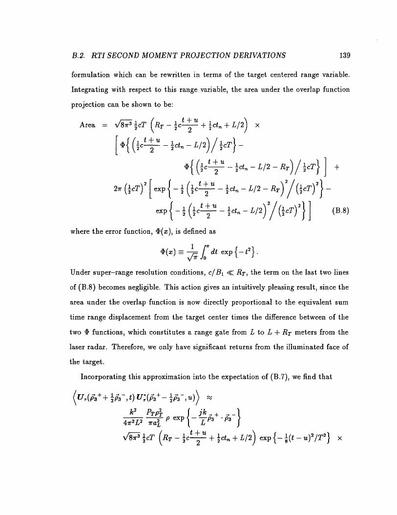
B.2. RTI SECOND MOMENT PROJECTION DERIVATIONS
formulation which can be rewritten in terms of the target centered range variable.
Integrating with respect to this range variable, the area under the overlap function
projection can be shown to be:
Area = 1 cT RTIC -2 U 2 ct + L/2) x
[,{ ( 2 -t -L/2) / cT} -
mu (2c + - ct -L/2-RT CT ] +
27(cT)[|exp {-I( t+u ctn-L/2-RT) 2(cT)2}-
exp { t+u 1 L/2) ( T) (B.8)
where the error function, (x), is defined as
(t)--va /dt exp{-t2}.
Under super-range resolution conditions, c/B1 < RT, the term on the last two lines
of (B.8) becomes negligible. This action gives an intuitively pleasing result, since the
area under the overlap function is now directly proportional to the equivalent sum
time range displacement from the target center times the difference between of the
two functions, which constitutes a range gate from L to L + RT meters from the
laser radar. Therefore, we only have significant returns from the illuminated face of
the target.
Incorporating this approximation into the expectation of (B.7), we find that
[P a , P3 , (Ur(i3 + 2P3 ,t) U:r( (P3 P3 ))
k2 PTP jk_+ _41r2L2 ra p exp -L P3 'P3
-cT (RT-C t 2 + ct + L/2) exp { -(t u)2/T2} x
139

APPENDIX B.
2 2
[{1(t+U - ct -L/2- - ]
where the factor on the last three lines is equal to the projected overlap area.
Taking the magnitude-squared of this result and integrating over the aperture
within a sum and difference coordinate formulation gives the final expression for
the received power covariance
Kpp(t,u) - 2 L a p2
(RT-C 2c + lct, + L/2) X
[41 ( 1 c + -1t, -L/)/ 2 CT-
2 2
We will now take advantage of the fact that this result is written in sum and difference
time coordinates.
As stated in §4.1.3, the quantity
{^eGY} JIdJd 1Lh(t -r)h(u-i)Kpp(r,1) = KPeckl'e(t,u) (B.10)
is the photodetector current covariance component attributable to received power fluc-
tuations, where h(t) is the detector impulse response. In this analysis, the impulse re-
sponse will be modelled by the low-pass Gaussian frequency response h(t) . e-i 2/B 2
where B is the nominal detector bandwidth.
Before calculating this covariance component, the above double-integral will be
rewritten in a power spectrum formulation which contrasts the relative contributions
between the sum and difference time-dependent factors. Switching to the sum and
140

B.2. RTI SECOND MOMENT PROJECTION DERIVATIONS
difference time coordinate systems:a!+ = (t + )
aC_ = t-U
and
3+ = (7 + )
the double-integral becomes
KSPecle(+ 1 +1 - )
hv eG rl Jh(a+ - + (a-- 3-)) h*(+0+ +- (a- -))
- {eG 2}Jd3+ Jd KP(+,) Jdfi H(fi)Jdf 2 H(f 2)
exp {+2rj [(a+ -P3+)(fi -f2) + (fi + f2)(a- -- )] }
where Kpp is the sum and difference formulation for the received power covariance
and H(f) A h(t).
Using the fact from equation (B.9) that Kp(p+, ,_) is separable in the (P+, 3_)
sum and difference time coordinates, we now write:
Kp(+,_- ) = Varpe(+) kpp(/-)
where the corresponding Fourier transform pairs are defined as follows:
Varp(/3+)Y
Vp(f)
kpp(P_) 4-, SPP(f).
141
Jdo- K±, (+ P-)

APPENDIX B.
Exchanging the time- and frequency-domain integrals, we have:
KSpckle(Ca + 1 a - 1
= { eGhv J dfi H(fi) JdfH*(f 2) Jdo+d Varp(fP+) e+2w(t+-+)(f-f2)
f dO_ kp(_ ) e +2j I (f, +fi)]
= { eG}Jdfi H(fi)Jdf, (f2) (fl - f2)ej' +(fl - f2)
Spp ( f + f2)) e27rij(fl+f2)/2
Switching to the surmr and difference coordinate system in the frequency domain:
f+ = (f + f2)
f- = - f2
we may finally write our desired formulation for the covariance double-integral in the
resulting rotated frequency-plane coordinate system:
KPcle(a+ + c a_, a+ - a_)2 1= {eG(h} Jdf+ J df_ H(f + 21 Hf - i f-)
Vp(f_ ) e2 ' jf - a+Spp(f+) e27rjf+a- (B.11)
= {eG} hv df+ Spp(f+) e- f+/B2 e2j f+ a - J df Vp(f_) ef-/4B 2e2f-a+
where, in the last line, we have substituted for the photodetector frequency response.
If we retain the assumption that the illumination pulse width T is sufficiently
small to provide meaningful resolution, every factor in the above expression has a
relatively large bandwidth except for Vp(f_). Assuming that e-f /4B2 is nearly unity
over the bandwidth of Vp(f) reduces the last integral to Varp(a+). Taking the
remaining integral with respect to df+ and converting back to the original t and u
142

B.2. RTI SECOND MOMENT PROJECTION DERIVATIONS
time coordinates, we then have:
KSpeckle(t u)// \~
{eGq 2 k4 a4
h L4
TB 1 exp {-(t
[i2 2
PT4T 2 (1 cT) 2aL
_u)2/2 }1- u 2 (RT 2- C + 2 ctn + L/2)
L/2- RT)/ 1CT}2
(B. 12)
where we have defined the system bandwidth to be
B1 _ I 14~r2T 2 + B 2
(B.13)
A similar analysis results in the following quantities for the thermal and shot-noise
contributions:
2kBTL
RLexp -(t-u) /, 22 } (B.14)
1 e 2 G2+z7
4 hvexp {-(t )2
[F{ (tct+U
aR PT p B (cT)
I1r2B2
I t(RT- + uRT-2c)(~ :":2- ctn-L/2)/
, 1 t+u 12
+ ct~ + L/2)
:t, - L/2
By rescaling the time axis to convert to range measured from the target center
and summing the shot-noise, speckle and thermal noise components in that order,
143
and
KSN(t, u)
x
1cT]i~ (B.15)
- ct, L/2 1cT -)2C~~~L~~n
Khermal(t' 1)
=
L.
4 -RT
=
2 - 2 2 t

APPENDIX B.
we have the result cited in (4.16),
1 e2 G2+"Y k2a2 PTpT ( xKp(ri, r2) .1 LB 2 a cT x
hv L 2 aL
(rl + r) exp -(r -r2)2 4r2B2 x
[ { ( y2 R)y T} {( 2 2)/1T} ]2 2
+ (eG12 (ka,) (Pi ) 2 (c2TB1 x
(-1 (r + r2)) exp -(r - r2 ) /4 2 } x[{ ((rl + T2) + RT)/ cT} - { ((r + r2))/cT} I 2
-+ w B 2kBTL exp {-(T- r2)/2 2 } (B.16)
where positive values of rl and r2 fall on the far side of the target. Note that this
result is separable into sum and difference range coordinates.
To demonstrate that inter-projection correlation is negligible, we will show that
the speckle coherence time is much shorter than the inter-pulse period in a typical
RTI imaging scenario. The speckle coherence time will be estimated by dividing the
speckle coherence length by the rate at which speckle lobes travel over the receiver
aperture.
We begin by defining the speckle covariance between the two position vectors
p3 and p3' spanning the receiver plane as KI(3, P 31 ,t) = ( [I(p 3,t) -(I(P3, t))
[I(3', t) - (I(3', t))] ) where the received field intensity I(pf3, t) is Ur(pi3, t) U(pa, t).
Expanding this definition and applying complex Gaussian moment factoring, we have
KII(P3, p3', t)= ( Ur( t),U(3 t) U) |
Equation (B.7) implies that the speckle lobe spatial structure will depend upon
both the surface reflectivity and roughness distributions as well as the shape of the
144

B.2. RTI SECOND MOMENT PROJECTION DERIVATIONS
illumination pulse striking the target at time t,. Since only a rough, order of mag-
nitude estimate of the coherence length is needed to validate our inter-projection
decorrelation assertion, for convenience sake, let us assume a constant target reflec-
tivity of p and constant spotlight mode illumination of the target (i.e., s(t) = 1).
Under these conditions, (B.7) reduces to
P ++ 2P3 ) U*(3 23)UrP3i .k2 PpT j f
4a2 L2 a, p exp - -P3 P3
k2 PT(2 Lk' - f jk n-
exp -L2 a 2 2 ( T ) P3fx{ ,12j42L 2 2 p2k2
during the time period when the laser illumination echo reaches the receiver.
Taking the magnitude-square and returning to the original P3 and P3' coordinates
results in the following time independent speckle spatial covariance:
4 P(4 2 2
KI I(,33,F31) = P247r 2L4 -r2a-4 a 2 /-aT RT
exp{-IP3- P3 p / 2_ RT
If we define the speckle decorrelation length to be pi =- jAp such that
KII(P3 + Ap, 3 - Ap)
KI I(Pw3, pf3)
then we compute the following length:
-1_ e
v'xAL 2 pTk2
P = -
145
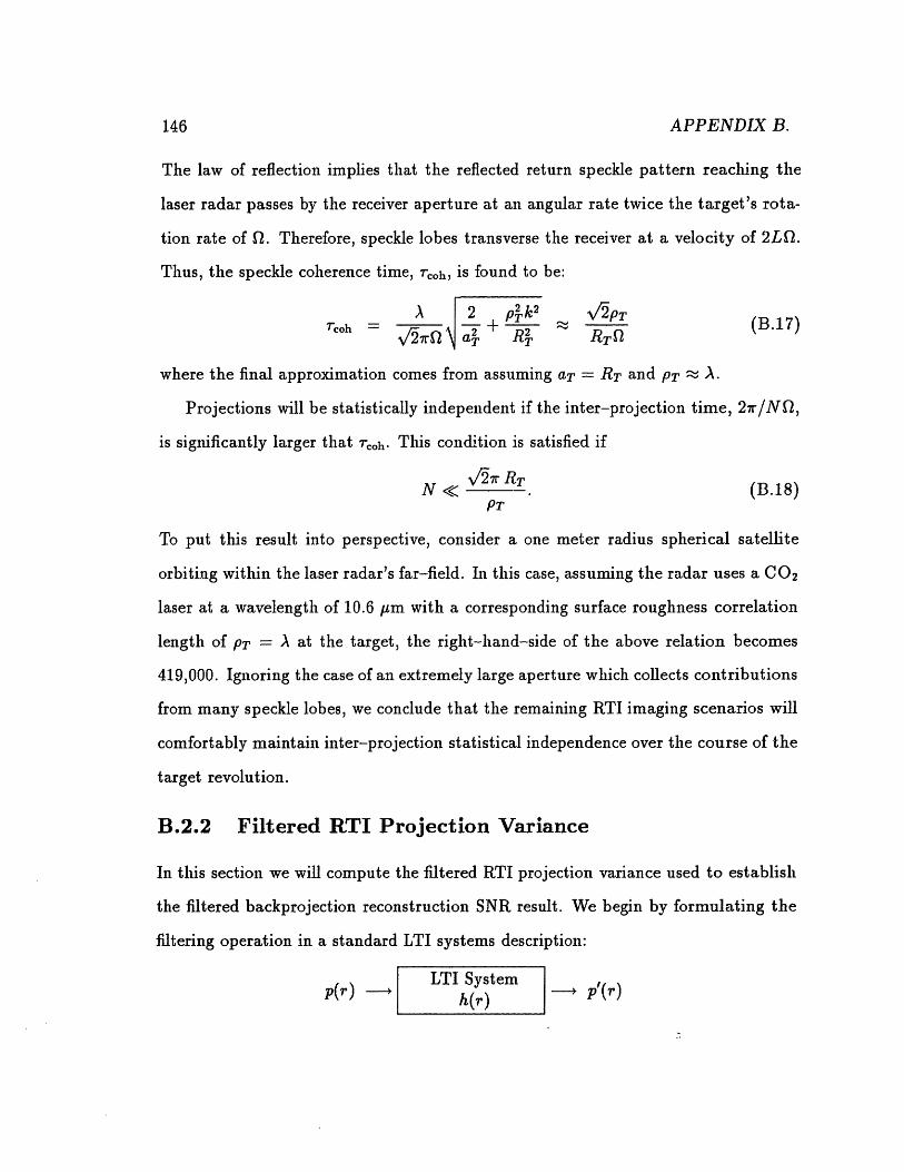
APPENDIX B.
The law of reflection implies that the reflected return speckle pattern reaching the
laser radar passes by the receiver aperture at an angular rate twice the target's rota-
tion rate of Q. Therefore, speckle lobes transverse the receiver at a velocity of 2L2.
Thus, the speckle coherence time, Tcoh, is found to be:
A ~2 p~,k' 2kpTTcoh A PT (B.17)J/7f aT 4 RTfl
where the final approximation comes from assuming aT = RT and PT - A.
Projections will be statistically independent if the inter-projection time, 27r/Nl,
is significantly larger that rcoh. This condition is satisfied if
N < RT (B.18)PT
To put this result into perspective, consider a one meter radius spherical satellite
orbiting within the laser radar's far-field. In this case, assuming the radar uses a CO2
laser at a wavelength of 10.6 pm with a corresponding surface roughness correlation
length of PT = A at the target, the right-hand-side of the above relation becomes
419,000. Ignoring the case of an extremely large aperture which collects contributions
from many speckle lobes, we conclude that the remaining RTI imaging scenarios will
comfortably maintain inter-projection statistical independence over the course of the
target revolution.
B.2.2 Filtered RTI Projection Variance
In this section we will compute the filtered RTI projection variance used to establish
the filtered backprojection reconstruction SNR result. We begin by formulating the
filtering operation in a standard LTI systems description:
p(r) | LTI System rh(r)
146

B.2. RTI SECOND MOMENT PROJECTION DERIVATIONS
where each projection is filtered by h(r) ,-- H(f) = If I to produce a new projection
p'(r) which is then backprojected establishing the inverse Radon transform operation.
Since the filtering operation is independent from projection to projection, we will still
assume that each p'(r) is statistically independent of all other filtered projections.
Our approach will build upon the projection covariance result derived in the previ-
ous subsection. Again, we will concentrate on the speckle contribution by formulating
this sum and difference range separable covariance component in a frequency-domain
description which easily allows us to calculate an approximation under super resolu-
tion conditions. Then the independent filtered thermal and shot-noise components
will be added to complete the filtered projection variance calculation.
The variance reformulation begins with the fact that varp,(r) = Kpp,(r, r) and
Kpxp(r1 r2) = Jdr Jdr'2 K,(r',r') h(r -r') h*(r2 -r').
For the speckle component, we apply the same covariance transformation procedure
as outlined from equation (B.10) to equation (B.11), which produces:
Kpe+e(+ r+ - r ) = Jdf+ Jdf_H(f+ + f ) H(f+-f )V(f_) e27rjr+f- (+) / 27+rVp(f-) e "j+ f-,pp(f+) es j f+ ' -
where (r+,r_) and (f+, f_) are the sum and difference range and spatial range fre-
quencies, respectively, defined in our previous pattern, and
Varp(r+) , Vp(f)
k(r_) Spp(f)
are the Fourier transform pairs of the sum and difference range-dependent factors in
the separable speckle projection covariance. Thus, the filtered projection variance at
147

APPENDIX B.
the point r is
Speckle( KSpeckle( + , - )
df+ J df H(f+ If-) H (f+ - f_) Vp(f) e27rjrf- (f+) (B.19)
Now applying the above reformulation result to our specific case of the inverse
Radon transform, we have H(f) = If which gives:
Spele/varpipt (r)
= Jdf+ dfI fi+2 fi2| Vp(f_)e27rtfp- (f+) (B.20)
= df+ df_ (f - fl) Vp(f_) e21f S(f+) -
2 x dff- df+ ( - f2) Vp(f_)e2rf Sf- (f+), (B.21)
Neglect
with the following specifications taken from (B.16),
kpp(r-) = exp47r2 B
Varp(r+) = (eGl) 2 () ( Tp2 p2 (½CT)2 TBi
( + [{(+ + RT)/cT}-{r / cT} 12
Suppose the laser radar is operating with a pulse width T chosen to provide useful
resolution in the range dimension. In the frequency domain, this assumption means
that the function Vp is much narrower than the function S. Therefore, in the
(f+, f_) Fourier plane, the function Vp(f_)Spp(f+) forms a narrow ridge-like feature
running along the f+-axis. Since the region of integration for the double-integral on
the second line of (B.21) overlaps a small part of the footprint of this "ridge," this
contribute to the total will be neglected.
148

B.2. RTI SECOND MOMENT PROJECTION DERIVATIONS
Performing the remaining distribution over the parenthetical term in the first line
of (B.21) gives:
Speckle (r) varpi¥ ( ' = j0f f+2 Spp(f+)
- jIdf+ Spp(f+)+00 ~~~21rjrf-jdf- V(f_ ) e2i f
j df_ f 2 V_(f ) e27rjrf_ 0 4
Substituting in the expressions for the separable components and their Fourier trans-
forms and performing the indicated integrations, we discuver that the expansion of
the second double-integral in equation (B.22) is insignificant under super-resolution
conditions.
Therefore, neglecting those terms, and adding the filtered thermal and shot-noise
variances computed via a similar set of manipulations, we have the result cited in
equation (4.18):
7re2 G2 +77 ka, PTPT 1 B3/C2 X
2 hvo a--L 2
(-r) [{(r + RT) /cT} - {r /cT)]
+2 (eG7) (kar) (PPTT) 2 2 ('cT)2 TB 3/C2 X
(_r)2 [ {(r + RT)/1cT}- {r/cT} ]
2kBTL B 3
RL C2 (B.23)
(B.22)
149
varprpp (r)

150 APPENDIX B.

Appendix C
Chapter 5 laid the ground work for the formulation of the heterodyne detector output
signal r(t) covariance. Assuming the limiting case of high local oscillator power, the
covariance of r(t) was separated into independent contributions from the shot-noise
n(t) covariance and the return signal y(t) covariance. Compared with the return
signal, the shot-noise n(t) was modelled as a relatively uncomplicated white noise
random process and was easily handled in the analysis. It is the goal of this appendix
to investigate the much more complicated return covariance, (y(u) y*(v), in order
to complete the mean and covariance calculations.
At the heart of these calculations is the assumption that the statistical behavior of
the return signal can be broken down into two largely independent factors correspond-
ing to physical processes which take place over relatively short- and long-term time
scales, respectively. These notions will be formalized mathematically by adopting the
Schell approximation [40] during the following calculations.
C.1 Heterodyne Signal Correlation
In tlhis section we detail the assumptions and modelling behind the computation of the
return signal correlation. To begin, we restate the return signal covariance expression
151

APPENDIX C.
derived in chapter 5:
(y(u) yj(v)) = J dJ d' PT 2(P) [(-,(P)]2 (T(, u)T*(, V)) (C.1)
where y(.) is the complex target return heterodyne component, PT is the transmitter
power, p( ) is the Gaussian beam complex spatial mode striking the target and
T(., * ) is the effective target reflectivity projected on to the T-plane.
As justified in Appendix B §1, we will break apart this double-integral into a sum
and difference formulation which exploits the rapid spatial decorrelation of tile return
phase. Therefore, we reformulate the above integral expression in our standard sum
and difference coordinate system:
P+ =2 (P + P )_ I -_
P- = p-p.
Applying this change of variables, we have
(y(u) y*(v))
1 -+1221
/drd fi PT kap exp { 2 ] p(p+(u, +v))exp 2 i+ }
exp {2jkF+ d -} exp{- + 1RT(t u)2 } (C.2)RT { 2 J
where the approximation sign comes about because we have made the following as-
sumptions in addition to coordinate transformation:
* As in the RTI Fraunhofer return calculation, individual returns from ~ PT-
sized surface patches only exhibit significant correlation during patch overlap,
and otherwise, make negligible contributions to the double-integral. Therefore,
under this condition, we have p p' which leads to lIp2 + (III2 ' iIl,+ p I'2l =
21p+ 12.
152

C.1. HETERODYNE SIGNAL CORRELATION
* Again, in the case of neighboring patches, the size of the regions over which
non-negligible contributions are made is on the order of the surface roughness
correlation length, PT. Since the value of this parameter is rather small, on
the order of a few wavelengths or so, we will assume that the target reflectivity
varies slowly over the patch extent, so that p(, u) Vp(', v), which gives:
p\(WU) p('v) p(p, 2(U + v)).
Since we are interested in investigating the speckle decorrelation behavior, let us
adopt the following time coordinates:
u = t+ x r (C.3)
v = t- 2T. (C.4)
The dummy time variable t accounts for the particular target aspect presented to
the laser radar during the observation time, while the time variable r will be used to
characterize the fast signal variations within the observation dwell time T. Thus, we
have
(y(t + 2r) y*(t- -))
d+ ; t74a4 7 P(P+t)ex P2 exp 2p 2T2 2
J d)_ exp{ X exp p2 }. (C.5)RT PT
We model spotlight-mode target illumination by assuming the last Gaussian term
on the second line is unity over the support of the transversely projected reflectance.
This action builds uniform target illumination into the model. Evaluating the second
153
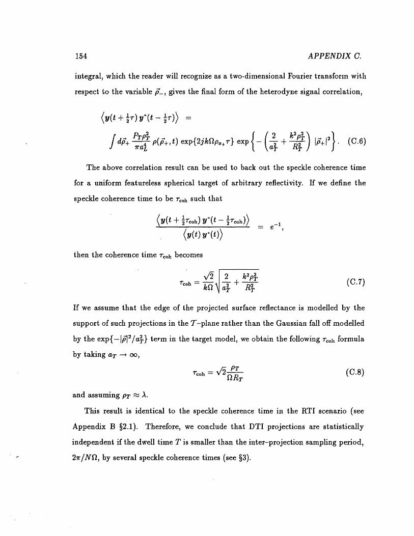
APPENDIX C.
integral, which the reader will recognize as a two-dimensional Fourier transform with
respect to the variable p_, gives the final form of the heterodyne signal correlation,
(y(t + 'r) y*(t - ))
/ d+ lr p(p+,t) exp{2jkfp.+(r} exp - + R, ) I/ + . (C.6)7raL aT R 1
The above correlation result can be used to back out the speckle coherence time
for a uniform featureless spherical target of arbitrary reflectivity. If we define the
speckle coherence time to be Toh such that
(y(t + 'rCOh) y(t - TcOh)) -1
(y(t) *(t))
then the coherence time rcoh becomes
X/2 2 k2 p2coh = k + (C.7)
kf2 +a R-
If we assume that the edge of the projected surface reflectance is modelled by the
support of such projections in the T-plane rather than the Gaussian fall off modelled
by the exp{-ip 2 /a4} term in the target model, we obtain the following rcoh formula
by taking aT -, oo,
7coh = V2 PT (C.8)flRT
and assuming PT A.
This result is identical to the speckle coherence time in the RTI scenario (see
Appendix B §2.1). Therefore, we conclude that DTI projections are statistically
independent if the dwell time T is smaller than the inter-projection sampling period,
27r/N, by several speckle coherence times (see §3).
154
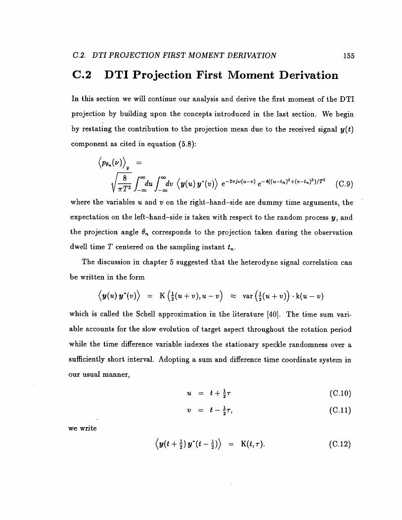
C.2. DTI PROJECTION FIRST MOMENT DERIVATION 155
C.2 DTI Projection First Moment Derivation
In this section we will continue our analysis and derive the first moment of the DTI
projection by building upon the concepts introduced in the last section. We begin
by restating the contribution to the projection mean due to the received signal y(t)
component as cited in equation (5.8):
(P,,(V))
where the variables u and v on the right-hand-side are dummy time arguments, the
expectation on the left-hand-side is taken with respect to the random process y, and
the projection angle 8,. corresponds to the projection taken during the observation
dwell time T centered on the sampling instant t.
The discussion in chapter 5 suggested that the heterodyne signal correlation can
be written in the form
(y(u) y*(v)) = K ((u + v), u-v) - var ((u + v)) k(u -v)
which is called the Schell approximation in the literature [40]. The time sum vari-
able accounts for the slow evolution of target aspect throughout the rotation period
while the time difference variable indexes the stationary speckle randomness over a
sufficiently short interval. Adopting a sum and difference time coordinate system in
our usual manner,
u = t-+ - (C.10)
v = t- -r, (C.11)
we write
(y(t+ 2)Y *(t - )) = K(t, ). (C.12)

APPENDIX C.
Therefore, using the covariance result derived in the previous section, the Fourier
transform of K(t, r) with respect to r is the power spectrum of the heterodyne signal
component at time indexed by the dummy variable t [40, 41]:
S(t,f) j= dr K(t, r) e - 2 If
PTP -00= j dr (y(t 2 - 2Rr I -
Io dr exp{2jkQp_+ r} exp{-2rjfr}0o0
= PPT J, dP+ (p- t) ( ( )R/
PT dp+ P (2 IJZp+) t) exp + b2 (C.13)
Two-DimensionalGaussian Window Function
where we have defined
b1= (C.14)0_,222 2
aT RT
Thus, for a fixed Doppler frequency f, which corresponds to a cross-range displace-
ment of r = Af/2Q meters, the power spectrum is proportional to a line-integral
along the p-axis. This formulation is a generalized Radon transform [27, §II.7]
indexed by the Doppler frequency. The integrand for the Radon transform is the sur-
face reflectivity transversely projected at time t onto the T-plane and weighted with
the same Gaussian metric discovered during the RTI analysis which models surface
roughness-aspect angle roll-off.
Thus, expressing the mean projection in the (t, r) sum and difference time coor-
156

157C.2. DTI PROJECTION FIRST MOMENT DERIVATION
dinates
(PO(v)),
,2i dt
dt~T2 oo
= 2foo_0
J00
J-00
dr K(t, r) e- 2wj e- 8(t- t )2 /T 2 e- 2r2 /T 2
dr ] df S(t, f)e 2jrfT' e- 27 j vr e-8(t- t )2/T 2 e-2.'2/T2
-oo
= K(t, )
-oo ooj. df j. dt S(t, f) e8It)./T L d-re2
df e- 7r2T2(f - ) 2/ 2 J dt S(t, f) e-8(t- t ) 2/T 2
oo
- s(t. f) dte- 8 ~2/ T 2
00
j(f-v)r e-2r2/T2
rT2 +00 (f_)2 1- df (t,., f) exp -(-v) 2 /2r-y-f s+f00 i 7 2T 2 (C.15)
where the final step the last integral was evaluated by applying the Schell approxima-
tion, i.e., assuming that S(t, f) varies slowly with respect to t about the dwell time
centered on sampling instant t,.
Completing the calculation by substituting (C.13) for S(t,, f) and rewriting the
above integral as a convolution, we have the final form of the mean projection (equa-
tion 5.13):
(P.(V))lv=2, / = [7T2/2exp { r2/k 2Q2T 2 }]
[PT f [ d p z pt' (r, pz) exp{-(pZ 2 + r2)/b2}]lraLJ-00
(C.16)

APPENDIX C.
C.3 DTI Second Moment Projection Derivations
In this section we will calculate the projection covariance for the DTI imaging system
assuming a low-contrast target reflectivity model and super-resolution conditions.
The following subsection details the calculation of the projection covariance. This
result is used in the second subsection to derive the filtered projection variance under
identical assumptions.
Before proceeding with these computations, we will use the results of the previous
section to demonstrate inter-projection statistical independence. This will be accom-
plished by showing that the sum of a typical dwell time T and speckle coherence
time is much shorter than the inter-projection sampling period. The upper bound
for T under permissible smearing conditions is found by setting the cross-range res-
olution cell dimension equal to the maximum target surface travel during the dwell
time. This gives the relation T < 1V/'/kTf for minimal smearing during projection
measurement. Therefore, the sum of both the maximum dwell and speckle coherence
times gives:
1 + V PT (C.17)v'rk RT f 2 RTf2
At infrared and visible wavelengths where A - PT and RT is on the order of meters,
this quantity is always smaller than the inter-projection sampling interval, 2r/NQ,
except in cases where thousands of projections are required.
In practical systems, projections will number less than approximately 100, and
thus, we will assume negligible inter-projection correlation. Therefore, the variance
between any two points along each projection is all that is required to compute the
reconstructed image variance.
158

C.3. DTI SECOND MOMENT PROJECTION DERIVATIONS
C.3.1 Projection Covariance
We begin b: defining the projection covariance between the two points corresponding
to the Doppler frequencies f and g along a DTI projection as ( [IL(f) 2 - (IL(f)l 2 )] -
[IL(g)l2 - (IL(g) 2)] )= Kpp(f, g). Since the heterodyne signal y is a circulo-complex
Gaussian random process, the application of complex Gaussian moment factoring
results in:
Kp(f, g) = (L(f)L"(f)L(g)L*(g)) -(p(f))(p(g))
= L(f) L*(g)) K(lf) L(g)) +
L(f) L*(f)) (L*(g) L(g)) +Becomes (p(f)) Becomes (p(g))
L(f) L(g)) L (f ) L(g) - (p(f))(p(g))=0 =0
L(f) L*(g)) 2
(C.18)
(C.19)
(C.20)
where moment factoring was used to expand equation (C.18) into (C.19), which after
simplification, gives the final result of (C.20).
At this point, it is helpful to recall that L( ) ultimately represents contributions
from local oscillator shot-noise n and speckle induced phase variations in the received
signal y. Since the heterodyne detector model presents these two random processes
as statistically independent in the high local oscillator power regime, we may now
write the expectation within the above magnitude-squared expression as
(L (f) L(g)) =
I+du0 dv (y(u) y*(v)) e-2rjfu +27rigv (8 1/2
- I(f g)
e-4(u-t,)2/T2 e-4(v-tn)2/T2 +e e +~~~~~~
159

APPENDIX C.
10du 1+d0 (n(u)n*(v)) e23rifue+2igv ( ) e-4(u-t.) 2 /T e-4(vIT
- 2(f, 9)
where the covariance of this nth projection is calculated for a projection dwell time
centered on the instant tn. Note that we have defined for the sake of future convenience
the first term in the above expansion as 11(f,g) and the second term as I2(f, g). Since
n(u) is a white noise process, we can immediately write the result:
I2(f, 9) = ho exp (f _ g)2 / 4 } exp {-27rj(f - g)t}. (C.21)
As with previous calculations involving the covariance of the received signal y(u),
we begin by taking expectations after converting to sum and difference time and
frequency coordinate systems in order to separate the short- and long-term statistical
behavior of the target return. Using the following transformations
t = 2(u + v)
= U-V
t= ½(f +g)
f-= f-g.to convert the expression for I1 (f, g) into an equivalent quantity denoted as I (f+, f_),
we have:
+00 +00 +00
Il(f+, f ) -= dt] d I df'S(t,f')e2 f'
= K(t, T)
exp {-27rj [(t +2+ -)(f. + f-) (t - )(f+ - -)] }
rT2 (.2
160

C.3. DTI SECOND MOMENT PROJECTION DERIVATIONS
where we have formulated the covariance of the received signal (y(u)y'(v)) in sum and
difference time coordinates and expressed this quantity, K(t, r), in terms of the single-
dimensional inverse Fourier transform of the power spectrum S(t, f') with respect
to f', the differential time-scale frequency. Cancelling common terms, exchanging
the order of integration and evaluating the resulting integral with respect to the
differential time coordinate r, we write:
8 1/2 +00 r+ (+00
= U+ ) ] dt]__dr ]__df'S(tf') e2rjr Iff +'-) (rT2 o t-00 J oexp {-27rj(f+7- + f_t)} e- s(t-t )2/ T2 e- 2r2 IT2
7 T2 J df' I dt S(t, f') e-r2ft e-8(t-t)2/T2
+0 dr e-2j(fs+-f') e-2r2 /T2
-00
2 X df' exp 1 (f+ _ fl)2
f dt S(t, f') e-8(tt" )2/T2 e- 2 1jf1 t (C.23)
S(tnf) I dte-8 C T -rjf-(t t)
where again in the final line, we introduce the assumption that observation dwell time
is sufficiently long to provide super-resolution. Evaluating the integral with respect
to t results in the following expression:
I(f+,f_) = 2 2exp- f/2 7r exp {-27rj(f - g)tn}
df' S(tn, f') exp {- (f+ - f')2 /r }. (C.24)
Convolution Integral
Except for the presence of the exponential and complex phase factors, the above result
is identical in form to equation (C.15) preceding the final projection mean description.
161

APPENDIX C.
Beginning with the expression for S(t, f'), equation (C.13), the power spectrum was
calculated for a low-contrast target with an overall reflectivity of p(z, y, z) = p, giving:
PTp'b A 1 \2 (f 2/)
S(t., f ) = p _exp { )(f)/b (C.25)
Substituting this result into equation (C.24), we have:
PTpTb2 A/2z~(+,7) a4 I1~(f~f-) = PT4 P/- exp {-2irj(f-g)t}exp {- f /r2T2 } exp {2 n f+2/ } (C.26)
where we have definedb2 1
o-2 - + (C.27)2 k2 f2 2T 2 '
The parameter o in some sense accounts for the apparent physical size of the target as
seen by the laser radar after taking into consideration the effects of surface roughness-
aspect angle and smearing due to finite dwell time T.
Therefore, the covariance of the random process L is obtained by converting back
to the original (f, g) coordinate system and summing both 1 and I2:
(L(f) L(g)) =
exp {- (f g)2 / 2 2 } exp {-2rj(f-g)t,} x
[ v + PTP b p exp{- () (f/ 4 }] (C.28)
Taking the magnitude-squared, we have the projection covariance:
Kp(f,g) = exp {-(fg) r2T2} x
hvo+ PTpb 2 A/2 exp {-2 2( )(f+g)2/42}] (C.29)+ p exp - (f + g)2 4o- (c.29)
162
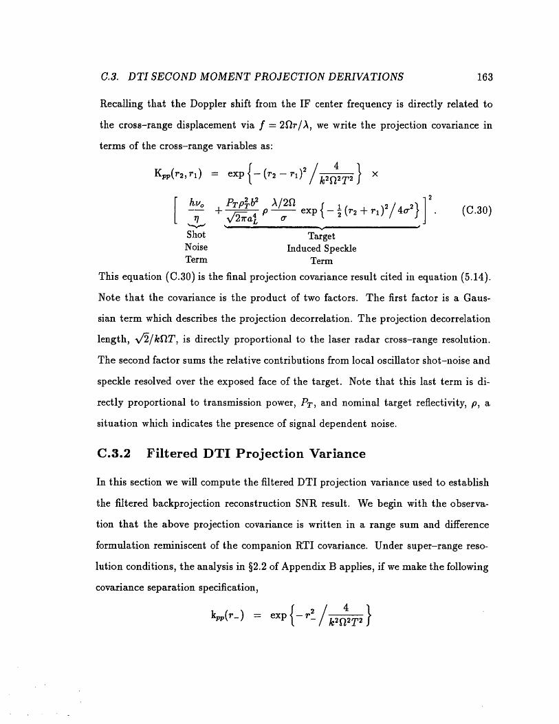
C.3. DTI SECOND MOMENT PROJECTION DERIVATIONS
Recalling that the Doppler shift from the IF center frequency is directly related to
the cross-range displacement via f = 2r/A, we write the projection covariance in
terms of the cross-range variables as:
4 + P exp (2 + r)2/42] (C.30)
Shot TargetNoise Induced SpeckleTerm Term
This equation (C.30) is the final projection covariance result cited in equation (5.14).
Note that the covariance is the product of two factors. The first factor is a Gaus-
sian term which describes the projection decorrelation. The projection decorrelation
length, /2/kT, is directly proportional to the laser radar cross-range resolution.
The second factor sums the relative contributions from local oscillator shot-noise and
speckle resolved over the exposed face of the target. Note that this last term is di-
rectly proportional to transmission power, PT, and nominal target reflectivity, p, a
situation which indicates the presence of signal dependent noise.
C.3.2 Filtered DTI Projection Variance
In this section we will compute the filtered DTI projection variance used to establish
the filtered backprojection reconstruction SNR result. We begin with the observa-
tion that the above projection covariance is written in a range sum and difference
formulation reminiscent of the companion RTI covariance. Under super-range reso-
lution conditions, the analysis in §2.2 of Appendix B applies, if we make the following
covariance separation specification,
k(r-) = exp {-r /k22T2}
163

164
Varp(r+)PTp]b2
+ v 4p' La
A/20O'
which gives in the following result cited in equation (5.16):
Ik2f2T2
varpp, (r) 82. varp(r).87r2
APPENDIX C.
exp{
(C.31)
1
2 hv,

Bibliography
[1] M. I. Sholnik, "Fifty years of radar," Proceedings of the IEEE, vol. 73, pp. 182-
197, February 1985.
[2] M. I. Skolnik, ed., Radar Handbook. New York: McGraw-Hill Publishing Com-
pany, 2nd ed., 1990.
[3] R. J. Doviak, D. S. Zrnic, and D. S. Sirmans, "Doppler weather radar," Proceed-
ings of the IEEE, vol. 67, pp. 1522-1553, November 1979.
[4] "FAA planning to deploy terminal weather radar," Aviation Week and Space
Technology, vol. 120, pp. 64-65, January 2, 1984.
[5] D. A. Boutacoff, "Backscatter radar extends early warning times," Defense Elec-
tronics, vol. 17, pp. 71-83, May 1985.
[6] D. Hughes, "Maine OTH-B completes development tests; GE to transfer system
to USAF," Aviation Week and Space Technology, vol. 132, pp. 52-53, April 9,
1990.
[7] "Magellan's radar images of Venus to unmask cloud-shrouded planet," Aviation
Week and Space Technology, vol. 131, pp. 113-115, October 9, 1989.
[8] S. D. Wall, "Venus unveiled," Astronomy, vol. 17, pp. 26-32, April 1989.
165

BIBLIOGRAPHY
[9] R. M. Gagliardi and S. Karp, Optical Communications. New York: John Wiley
and Sons, 1976.
[10] J. H. Shapiro, B. A. Capron, and R. C. Harney, "Imaging and target detection
with a heterodyne-reception optical radar," Applied Optics, vol. 20, pp. 3292-
3313, 1981.
[11] J. C. Dainty, ed., Laser Speckle and Related Phenomena. Vol. 9 of Topics in
Applied Physics, New York: Springer-Verlag, 2nd ed., 1984. Chapter 2.
[12] J. H. Shapiro, "Target-reflectivity theory for coherent laser radars," Applied Op-
tics, vol. 21, pp. 3398-3407, September 15, 1982.
[13] J. H. Shapiro, "Correlation scales of laser speckle in heterodyne detection," Ap-
plied Optics, vol. 24, pp. 1883-1888, June 15, 1985.
[i4] D. M. Papurt, J. H. Shapiro, and R. C. Harney, "Atmospheric propagation effects
on coherent laser radars," Proceedings of SPIE, vol. 300, pp. 86-99, 1981.
[15] D. M. Papurt, J. H. Shapiro, and S. T. Lau, "Measured turbulence and speckle
effects in laser radar target returns," Proceedings of SPIE, vol. 415, pp. 166-178,
1983.
[16] R. C. Harney and R. J. Hull, "Compact infrared radar technology," Proc. Soc.
Photo-Opt. Instrum. Eng., vol. 227, pp. 162-170, 1980.
[17] M. B. Mark, "Multipixel, multidimensional laser radar system performance,"
Ph.D. thesis, Dept. of Elect. Engr. and Computer Sci., MIT, 1986.
[18] M. B. Mark and J. H. Shapiro, "Multipixel, multidimensional laser radar system
performance," Proceedings of SPIE, vol. 783, pp. 109-122, 1987.
166

BIBLIOGRAPHY
[19] S. M. Hannon, "Detection processing for multidimensional laser radars," Ph.D.
thesis, Dept. of Elect. Engr. and Computer Sci., MIT, 1989.
[20] D. L. Mensa, S. Halevy, and G. Wade, "Coherent Doppler tomography for mi-
crowave imaging," Proceedings of the IEEE, vol. 71, pp. 254-261, February 1983.
[21] D. C. Munson, Jr., J. D. O'Brien, and W. K. Jenkins, "A tomographic for-
mulation of spotlight-mode synthetic aperture radar," Proceedings of the IEEE,
vol. 71, pp. 917-925, August 1983.
[22] F. K. Knight, S. R. Kulkarni, R. M. Marino, and J. K. Parker, "Tomographic
techniques applied to laser radar reflective measurements," The Lincoln Labora-
tory Journal, vol. 2, pp. 143-160, Summer 1989.
[23] F. K. Knight, D. I. Klick, D. P. Ryan-Howard, J. R. Theriault, Jr., B. K. Tussey,
and A. M. Bechman, "Two-dimensional tomographs using range measurements,"
Proceedings of SPIE, vol. 999, pp. 269-280, 1988.
[24] R. M. Marino, "Tomographic image reconstructions from laser radar reflective
projections," Proceedings of SPIE, vol. 999, pp. 248-268, 1988.
[25] G. T. Herman, ed., Image Reconstructions from Projections. Vol. 32 of Topics
in Applied Physics, New York: Springer-Verlag, 1979.
[26] A. Macovski, Medical Imaging Systems. Englewood Cliffs, New Jersey: Prentice-
Hall, Inc., 1983.
[27] F. Natterer, The Mathematics of Computerized Tomography. New York: John
Wiley and Sons, 1986.
167

BIBLIOGRAPH Y
[28] D. Park, "High-Resolution Laser Radar Performance Analysis," Ph.D. thesis,
Dept. of Elect. Engr. and Computer Sci., MIT, 1988.
[29] J. W. Goodman, Introduction to Fourier Optics. New York: McGraw-Hill, 1968.
[30] D. L. Fried, "Statistics of the laser radar cross section of a randomly rough
target," J. Opt. Soc. Am., no. 11, pp. 1150-1160, 1976.
[31] J. C. Leader, "An analysis of the frequency spectrum of laser light scattered from
moving rough objects," J. Opt. Soc. Am., vol. 67, pp. 1091-1098, August 1977.
[32] N. George, "Speckle from rough, moving objects," J. Opt. Soc. Am., vol. 66,
pp. 1182-1194, November 1976.
[33] J. C. Erdmann and R. I. Gillert, "Speckle field of curved, rotating surfaces of
gaussian roughness illuminated by a laser light spot," J. Opt. Soc. Am., vol. 66,
pp. 1194-1204, November 1976.
[34] J. H. Shapiro, "Lecture Notes for 6.453 Optical Detection and Communication,"
M.I.T. Electrical Engineering and Computer Science Dept., Cambridge, Mas-
sachusetts, 1982.
[35] P. Richardus and R. K. Adler, Map Projections. Amsterdam: North-Holland,
1972.
[36] A. E. Siegman, "The antenna properties of optical heterodyne receivers," Proc.
IEEE, vol. 54, p. 1350, 1966.
[37] S. R. Kulkarni, A. S. Lele, and M. F. Reily, "Qualitative Differences Between
Tomographic Reconstructions from Range-Resolved verses Doppler-Resolved
168
BIBLIOGRAPHY
Data," Project Memorandum No. 52PM-ODT-0042, M.I.T. Lincoln Laboratory,
Lexington, Massachusetts, 1989.
[38] A. L. Kachelmyer, "Range Doppler imaging: waveforms and receiver design,"
Proceedings of SPIE, vol. 999, pp. 138-161, 1988.
[39] A. L. Kachelmyer, "Range-Doppler imaging with a laser radar," The Lincoln
Laboratory Journal, vol. 3, no. 1, pp. 87-118, 1990.
[40] A. C. Schell, "A technique for the determination of the radiation pattern of a
partially coherent aperture," IEEE Transactions on Antennas and Propagation,
vol. 15, pp. 187-188, 1967.
[41] D. L. Snyder, J. A. O'Sullivan, and M. I. Miller, "The use of maximum likelihood
estimation for forming images of diffuse radar targets from delay-Doppler data,"
IEEE Transactions on Information Theory, vol. 37, pp. 536-548, May 1989.
169

Biographical Note
Bradley Thomas Binder was born in Yankton, South Dakota on April 6, 1960. In
1983 he graduated from the University of Nebraska with a B.S.E.E. degree with high
distinction and was named a University Chancellor's Scholar. Entering the Dept.
of Electrical Engineering and Computer Science at the Massachusetts Institute of
Technology in 1984, he was supported by a National Science Foundation Graduate
Fellowship in obtaining his S.M.E.E. and Electrical Engineer's degree in 1987 while a
member of the Research Laboratory of Electronics. In the beginning of his graduate
education in 1984, and finally in 1988, he was a Dept. Teaching Assistant before ac-
cepting an appointment as a Research Assistant with the Laser Radar Measurements
Group at the M.I.T. Lincoln Laboratory. His research has appeared in the IEEE
Transactions on Communications.
Mr. Binder is a staff member with the M.I.T. Lincoln Laboratory Battlefield
Surveillance Group in Lexington, Massachusetts. He is engaged to Miss Joellen
DiRusso of Dedham, Massachusetts.
170