Layer-Parallel Training of Deep Residual Neural Networks

Layer-Parallel Training of Deep Residual Neural Networks

S. Gunther∗1, L. Ruthotto†2, J.B. Schroder3, E. C. Cyr‡4, and N.R. Gauger1

1Scientific Computing Group, TU Kaiserslautern, Germany2Department of Mathematics and Computer Science, Emory University, Atlanta, GA, USA3Dept. of Mathematics and Statistics, University of New Mexico, Albuquerque, NM, USA

4Computational Mathematics Department, Sandia National Laboratories, Albuquerque,NM, USA

December 10, 2018

Abstract

Residual neural networks (ResNets) are a promising class of deep neural networks that haveshown excellent performance for a number of learning tasks, e.g., image classification and recog-nition. Mathematically, ResNet architectures can be interpreted as forward Euler discretizationsof a nonlinear initial value problem whose time-dependent control variables represent the weightsof the neural network. Hence, training a ResNet can be cast as an optimal control problem ofthe associated dynamical system. For similar time-dependent optimal control problems arisingin engineering applications, parallel-in-time methods have shown notable improvements in scal-ability. This paper demonstrates the use of those techniques for efficient and effective trainingof ResNets. The proposed algorithms replace the classical (sequential) forward and backwardpropagation through the network layers by a parallel nonlinear multigrid iteration applied tothe layer domain. This adds a new dimension of parallelism across layers that is attractivewhen training very deep networks. From this basic idea, we derive multiple layer-parallel meth-ods. The most efficient version employs a simultaneous optimization approach where updatesto the network parameters are based on inexact gradient information in order to speed up thetraining process. Using numerical examples from supervised classification, we demonstrate thatour approach achieves similar training performance to traditional methods, but enables layer-parallelism and thus provides speedup over layer-serial methods through greater concurrency.

1 Introduction

One of the most promising areas in artificial intelligence is deep learning, a form of machine learningthat uses neural networks containing many hidden layers [4, 42]. Even though neural networks date

∗Corresponding author: [email protected]†LR is supported by the US National Science Foundation awards DMS 1522599 and DMS 1751636‡Sandia National Laboratories is a multimission laboratory managed and operated by National Technology & Engi-

neering Solutions of Sandia, LLC, a wholly owned subsidiary of Honeywell International Inc., for the U.S. Departmentof Energy’s National Nuclear Security Administration under contract DE-NA0003525. The views expressed in thearticle do not necessarily represent the views of the U.S. Department of Energy or the United States Government.

1

back at least to the 1950’s [46], recent advances in computer hardware as well as the availability ofever larger data sets have enabled and fueled the success of modern machine learning techniques.Since then, deep neural networks (DNNs), and in particular deep residual networks (ResNets) [34],have been breaking human records in various contests and are now central to technology such asimage recognition [36, 41, 42] and natural language processing [6, 15, 39].

The abstract goal of machine learning is to model a function f : Rn ×Rp → Rm and train itsparameter θ ∈ Rp such that

f(y,θ) ≈ c (1.1)

for input-output pairs (y, c) from a certain data set Y ×C. Depending on the nature of inputs andoutputs, the task can be regression or classification. When outputs are available for all samples,parts of the samples, or are not available, this formulation describes supervised, semi-supervised,and unsupervised learning, respectively. The function f can be thought of as an interpolation orapproximation function.

In deep learning, the function f includes a DNN that aims at transforming the input data. In thecase of feed forward networks, this process is called forward propagation and for an N -layer neuralnetwork one starts with u0 = y and proceeds with un+1 = Φ(un,θn) for all n = 0, 1, . . . , N − 1,which propagates the input data through all layers of the network. Here, the vector of parametersθ ∈ Rp is partitioned into parameters for each layer, θ0,θ1, . . . ,θN−1. In this paper, we consider aspecial type of forward propagation given by ResNets [34], for which the forward propagation reads

un+1 = un + hF (un,θn), (1.2)

where h > 0 is a constant and the layer function F consists of relatively simple operations, such asaffine linear mappings parameterized by the parameters θn and nonlinear element-wise activationfunctions. While we restrict the discussion to feed-forward networks for supervised classification,the layer-parallel integration can be extended to some recurrent learning tasks and, when the outputdata is replaced with a reward function, reinforcement learning (for general introductions to thisfield see, e.g., [22, 2, 28]).

The training problem consists of finding the parameters θn such that (1.1) is satisfied forelements from a training data set but also holds for previously unseen data from a validation data setwhich has not been used during training. The former objective is commonly modeled as an expectedloss and optimization techniques are used to find the parameters that minimize the loss. Usingnetworks with a sufficient number of layers and parameters and adequate minimization techniques,it is typically possible to obtain a solution with an arbitrarily low expected loss. However, similar topolynomial interpolation, this strategy may result in overfitting and minimizers may perform poorlyon data not used during the training, in other words, the network fails to generalize. Designinglearning strategies that ensure generalization is a subject of current research.

Despite the rapid methodological developments, compute times for the training of state-of-the-art DNNs can still be prohibitive, measured in the order of hours or days, involving hundreds oreven thousands of layers and millions or billions of network parameters [16, 40]. There is thus agreat interest in increasing parallelism to reduce training runtimes. Common approaches involvedata- and model-parallelism. Data-parallelism refers to the idea of distributing elements of thetraining data set onto multiple compute units. Synchronous and asynchronous data-parallel trainingalgorithms have been developed to coordinate the network parameter updates [37, 1]. In contrast,model-parallelism refers to partitioning the different layers of the network and its parameters todifferent compute units. Model parallelism has traditionally been used when the network dimension

2

exceeds available memory of a single compute unit. Often, a combination of both approaches isemployed [33, 16]. However, none of the above approaches to parallelism tackle the scalabilitybarrier created by the serial propagation of data elements through the network layers itself. Ineither above approach, each subsequent layer can process information only after the previous layerhas finished its computation. As a result, training runtimes scale linearly with the number oflayers. As current state-of-the-art networks tend to increase complexity by adding more and morelayers (see, e.g., the ResNet-1001 with 1001 layers and 10.2 million weights in [35]), the serial layerpropagation creates a serious bottleneck for fast and scalable training algorithms that leveragemodern HPC architectures.

In this paper, we address the above scalability barrier by introducing concurrency across thenetwork layers. To this end, we replace the serial data propagation through the network by anonlinear multigrid method that treats layer chunks simultaneously and thus enables full layer-parallelism. Our goal is to have a training methodology scalable in the number of layers, e.g.,doubling the number of layers and the number of compute resources should result in a near constantruntime. To achieve this, we leverage recent advances in parallel-in-time integration methods forunsteady differential equations [23]. Clearly, the forward propagation through a ResNet (1.2) canbe seen as a discretization of a time-dependent ordinary differential equation (ODE), which was alsoobserved in [32, 18]. Based on this interpretation, we employ a multigrid reduction in time approach[19, 20] that recursively divides the time domain – which, in this interpretation, corresponds to thelayer domain – into multiple time chunks that can be processed in parallel on different computeunits. Coupling of the chunks is achieved through a coarse-grid correction scheme that propagatesinformation across chunk interfaces on a coarser time- (i.e. layer-) grid. The method can be seen asa parallelization of the model, however we employ full model-parallelism on the algorithmic level,processing layer chunks simultaneously within the iterative multigrid scheme thus breaking thetraditional layer-serial propagation. At convergence, the iterative multigrid scheme solves the sameproblem as a layer-serial method and it can thus be integrated into any common gradient-basedoptimization technique to update the network parameters, such as the stochastic gradient descent(SGD) or other batch approaches. Further, it can be applied in addition to any data-parallelismacross the data set elements. Runtime speedup over traditional layer-serial methods can be achievedthrough the new dimension of parallelization across layers enabling greater concurrency.

The addition of layer-parallelism allows for ResNets to take advantage of large machines cur-rently programmed with message-passing style parallelism. The use of such large machines inconjunction with a multilevel training algorithm scalable in the number of layers, opens the doorto training networks with thousands, or possibly even millions of layers. We demonstrate the fea-sibility of such an approach by using the parallel-in-time package XBraid [50] with a ResNet onlarge clusters. Additionally, the non-intrusive approach of XBraid would allow for any node-leveloptimizations (such as those utilizing GPUs) to be used.

The iterative nature of the multigrid approach further enables the use of simultaneous optimiza-tion algorithms for training the network. Simultaneous optimization methods have been widely usedfor PDE-constrained optimization, where they show promise for reducing the runtime overhead ofthe optimization when compared to a pure simulation of the underlying PDE (see e.g. [7, 51, 5]and references therein). They aim at solving the optimization problem in an all-at-once fashion,updating the optimization parameters simultaneously while solving for the time-dependent systemstate. Here, we apply the One-shot method [9, 31] to solve the training problem simultaneouslyfor the network state and parameters. In this approach, network parameter updates are based on

3

inexact gradient information resulting from early stopping of the layer-parallel multigrid iteration.The paper is structured as follows: Section 2 gives an introduction to the deep learning op-

timization problem and its interpretation as an optimal control problem. Further, it discussesnumerical discretization of the optimal control problem and summarizes necessary conditions foroptimality as well as commonly used numerical optimization techniques. We then introduce thelayer-parallel multigrid approach replacing the forward and backward propagation through thenetwork in Section 3. Section 4 focuses on the integration of the layer-parallel multigrid schemeinto conventional as well as simultaneous optimization methods. Numerical results demonstratingthe feasibility and runtime benefits of the proposed layer-parallel multigrid scheme as well as itsutilization in simultaneous training are presented in Section 5.

2 Deep Learning as a Dynamic Optimal Control Problem

In this section, we present an optimal control formulation of a supervised classification problemusing a deep neural network. Limiting the discussion to this specific task allows us to provide aself-contained mathematical description. We note that our techniques can be extended to otherlearning tasks, e.g., semi-supervised learning or auto-regression and refer to [28] for a comprehensiveoverview of deep learning techniques.

2.1 Optimal Control Formulation

In supervised classification, we are given some feature vectors y1,y2, . . . ,ys ∈ Rn (examples) andassociated class probability vectors c1, c2, . . . , cs ∈ ∆nc , where ∆nc denotes the unit simplex in Rnc .The j-th component of ck represents the probability of example yk belonging to the j-th class.

The learning problem aims at training a function that approximates the feature-to-class map-ping. In other words, we seek to find a function f(·,θ) and its parameter (or weights) θ suchthat

f(yk,θ) ≈ ck, for all k = 1, 2, . . . , s.

In order to classify the feature vectors into specific classes, a hypothesis function is required thatpredicts the class probabilities of each example. Here, we limit ourselves to multinomial regressionmodels, which are common in deep learning. To this end, we assume that the weights θ can bepartitioned into a matrix W ∈ Rnc×n and a bias vector µ ∈ Rnc . For a generic example y, thefollowing softmax hypothesis function can then be considered:

s(y,W,µ) =1

e>ncexp(z)

exp(z), z = Wy + µ, (2.3)

where enc ∈ Rnc is a vector of all ones and exp is the exponential function.1 It is easy to verifythat s(y,W,µ) will be in the unit simplex and can thus be seen as a discrete probability and iscomparable to the corresponding class probability vector c. To measure the performance of theclassifier, we use the cross entropy loss function

`(y,W,µ, c) = −c> log(s(y,W,µ)) (2.4)

= −c>z + log(e>ncexp(z)). (2.5)

1Note, that the softmax hypothesis function is invariant to scalar shifts in z. Thus, without loss of generality weassume that the entries in z are non-negative, which avoids overflow.

4

Minimizing the average loss function over many examples with respect to W and µ corre-sponds to finding hyperplanes that approximately partition the feature space into nc subsets. Themultinomial regression model will however only be effective when the different classes can be ap-proximately separated using hyperplanes. If this assumption is not valid, it is sometimes possibleto apply nonlinear transformations to the example data that improve the performance of the aboveclassification. The key idea in deep learning is to represent this nonlinear transformation usinga neural network consisting of a concatenation of many hidden layers. Each layer transforms theinput features using relatively simple operations: Each layer applies affine transformations andelement-wise nonlinearities, whose parameters need to be learned along with the weights and biasof the classifying softmax function.

A powerful class of networks that has been shown to be very successful in many benchmarktasks are Residual Neural Networks (ResNets) [34]. In an abstract form, an N -layer residual neuralnetwork reads

un+1 = un + hF (un,θn), for n = 0, 1, . . . , N − 1, with u0 = Fin(y,θin). (2.6)

The layer transformations F and Fin consist of an affine linear transformations and element-wisenonlinearities that are parameterized by the entries in θ0, . . . ,θN−1, and θin, respectively. Thereare several options to model these functions. For simplicity, we consider the single layer perceptronmodels

F (u,θ) = σ(K(θ(1))u + Bθ(2)), and Fin(y,θ) = σ(Kin(θ(1))y + Binθ(2)), (2.7)

where σ : R → R is a nonlinear activation function that is applied component-wise, e.g., σ(x) =tanh(x) or σ(x) = max{x, 0}. Here, the weight vectors θn are partitioned into one part thatdefines a linear operator K and another part that represents coefficients of a bias with respectto columns of the given matrices B and Bin. In this work, we assume that the linear operatorsK(·) are either dense matrices or correspond to convolutional operators (see [43]) parametrized byθ(1), whose entries we determine in the training. However, our method can be extended to otherparameterizations (e.g., antisymmetric matrices to enforce stability [32]). While K(·) needs to bea square matrix we use a non-square model for the operator Kin(·) to increase the dimensionalityof the dataset, which helps in the training.

Considering a small but positive h in (2.6), it is intuitive to interpret ResNets as a forwardEuler discretization of the initial value problem

∂tu(t) = F (u(t),θ(t)), t ∈ [0, T ], with u(0) = Fin(y,θin). (2.8)

In this formulation, t is an artificial time that refers to the propagation of the input features throughthe neural network. The final time T and the norm of F (u(t),θ(t)) are loosely related to the depthof the neural network.

Replacing the original features y in (2.3) by the state of (2.8) at the final time T , leads to thefinal model function

f(y,θ) = s(u(T ),W,µ), where u solves (2.8).

Minimizing the empirical cross entropy loss function leads to the continuous-in-time optimal control

5

problem

minu1,...,us,θ,W,µ

1

s

s∑k=1

`(uk(T ),W,µ, ck) +R(θ(t),W,µ) (2.9)

subject to ∂tuk(t) = F (uk(t),θ(t)), ∀t ∈ [0, T ], (2.10)

uk(0) = Fin(yk,θin). (2.11)

The objective function consists of the average loss over all examples, hence approximating its ex-pected value, and an additional regularization term denoted by R that involves all network parame-ters θ(t) and the classification weights and biases W,µ. In conventional deep learning approaches,R typically applies a Tikhonov regularization that penalizes “large” network and classification pa-rameters, measured in a chosen norm. Within the time-continuous optimal control interpretation,we additionally penalize the time derivative of θ(t) in order to ensure weights that vary smoothly intime. This is an important ingredient for stability analysis [32]. Another task for the regularizationfunction is to avoid over-fitting, which means that the optimal parameters perform very well for thetraining data but perform poorly on new data. In contrast to many applications in optimal control,in most applications of machine learning it is therefore not desirable to minimize the loss over thetraining data to a very high accuracy, but rather to stop the iterative minimization method early;see discussions in Sec. 2.4 and [11].

To gauge the network’s performance on unseen data it is common to set aside parts of the dataas a validation set and monitor the loss over this set while adjusting hyper-parameters, e.g., thenetwork size, layer designs, regularization parameters, optimization parameters.

2.2 Discretization of the Optimal Control Problem

We solve the continuous-in-time optimal control problem in a first-discretize-then-optimize fashion.For simplicity, we discretize the control θ(t) and the states u(t) at regularly spaced time pointstn = n · h, where h = T/N and n = 0, 1, . . . , N . This leads to the discrete control problem

minu0

1,...,u0s,...,u

N1 ,...,uN

s ,W,µ,θJ(uN

1 , . . . ,uNs ,W,µ,θ) (2.12)

subject to un+1k = Φ(un

k ,θn), ∀n = 0, . . . , N − 1 (2.13)

u0k = Fin(yk,θin), (2.14)

where θ collects all network control parameters that need to be learned, θ := (θ0, . . . ,θN−1,θin)and J denotes the discretized objective function

J(uN1 , . . . ,u

Ns ,W,µ,θ) :=

1

s

s∑k=1

`(uNk ,W,µ, ck) +R(θ,W,µ) (2.15)

In this general description, Φ can denote any layer-to-layer propagator which maps data un to thenext layer. In case of a forward Euler discretization, it reads

Φ(u,θ) = u + hF (u,θ). (2.16)

giving the ResNet propagation as in (2.6). However, the time-continuous interpretation of thenetwork propagation permits to employ other, possibly more stable, discretization schemes, see

6

[32] and thus opens the door for new architecture designs. It also allows for discretization of thecontrols, θ, and states, u, at different time points, which can improve the efficiency and is thesubject of further research. Further, numerical advances for solving the corresponding optimalcontrol can be leveraged, such as the time-parallel approach which is discussed in this paper.

2.3 Necessary Optimality Conditions

The necessary conditions for optimality of the discrete, equality-constrained optimization problem(2.12)-(2.14) can be derived from the associated Lagrangian function

L :=J(uN1 , . . . ,u

Ns ,W,µ,θ) +

s∑k=1

[N−1∑n=0

(un+1k

)T (Φ(un

k ,θn)− un+1

k

)+(u0k

)T (Fin(yk,θin)− u0

k

)](2.17)

where unk denote the so-called adjoint states for layer n = 0, . . . , N and example k = 1, . . . , s.

Optimal points of the problem are saddle points of the Lagrangian function (see e.g. [45]), thusequating its partial derivatives with respect to u0, . . . ,uN , u0 . . . , uN , and θ0, . . . ,θN ,θin,W,µ tozero yields the following necessary conditions for optimality:

1. State equations

un+1k = Φ(un

k ,θn), ∀n = 0, . . . , N − 1, (2.18)

with u0k = Fin(yk,θin), for all k = 1, . . . , s (2.19)

2. Adjoint equations

unk = (∂uΦ(un

k ,θn))T un+1

k , ∀n = 0, . . . , N − 1, (2.20)

with uNk =

1

s

(∂u`(u

Nk ,W,µ, ck)

)Tfor all k = 1, . . . , s (2.21)

3. Design equations

0 =

s∑k=1

(∂θnΦ(unk ,θ

n))T un+1k + (∂θnR(θ,W,µ))T ∀n = 0, . . . , N − 1 (2.22)

0 =

s∑k=1

(∂θinFin(yk,θin))T u0

k + (∂θinR(θ,W,µ))T (2.23)

0 =1

s

s∑k=1

(∂W`(uN

k ,W,µ, ck))T

+ (∂WR(θ,W,µ))T (2.24)

0 =1

s

s∑k=1

(∂µ`(u

Nk ,W,µ, ck)

)T+ (∂µR(θ,W,µ))T (2.25)

Here, subscripts denote partial derivatives, ∂x = ∂∂x . The state equations correspond to the forward

propagation of input data yk through the network layers. The adjoint equations propagate partialderivatives with respect to the network states backwards through the network layers, starting

7

from a terminal condition at N equal to the local derivative of the loss function. In a time-continuous setting, the adjoint equations correspond to the discretization of an additional adjointdynamical system for propagating network state derivatives backwards in time.2 We note thatsolving the above adjoint equations backwards in time is equivalent to the backpropagation methodthat is established within the deep learning community for computing the network gradient [43].It further corresponds to the reverse mode of automatic differentiation [29]. The adjoint variablesare utilized in the right-hand-side of the design equations, which then form the so-called reducedgradient. For feasible state and adjoint variables, the reduced gradient holds the total derivative,i.e. the sensitivity, of the objective function with respect to the controls. It is thus used withingradient-based optimization methods for updating the network controls.

Training a residual network corresponds to the attempt of solving the above set of equationsfor the special choice of Φ being the forward Euler time-integration scheme. However, the aboveequations, as well as the discussions in the remainder of this paper, are general, in the sense thatany other layer-to-layer propagator Φ can be utilized that corresponds to the discretization of thedynamical system (2.8).

Remark 1 The adjoint equations depend on the primal states unk themselves. Therefore, those

states need to be either stored during forward propagation, or recomputed while solving the adjointequations. Hybrid approaches like the check-pointing method have been developed within the op-timal control and unsteady PDE-constrained optimization community, which compromise memoryconsumption with computational complexity (see, e.g., [49]). Memory-free methods using reversiblenetworks were first proposed for general dynamics in [27]. However, as shown in [14], not allarchitectures that are reversible algebraically are forward and backward stable numerically. Thismotivates limiting the forward propagation to stable dynamics, e.g., inspired by hyperbolic systems.

2.4 Common Gradient-based Training Techniques

Due to the large-scale and stochastic nature of the learning problem (2.12), it is common touse stochastic approximation schemes, such as variants of the stochastic gradient descent (SGD)method, for updating the controls within a gradient-based optimization iteration. These methodsassemble gradient information from a (randomly chosen) subset of the training data, i.e. the sumover k in the design equations cover only a subset k ∈ S ⊂ {1, . . . , s} of the full data, called a batch.The size of the batch can be as small as one, where a different example is randomly chosen in eachiteration of the SGD method. While they reduce the cost of gradient evaluations, small batch sizescomplicate their data-parallel implementation when more computational resources than examplesin the batch are available. An alternative are stochastic average approximation (SAA) schemesthat allow for larger batch sizes and the straightforward incorporation of second-order information,such as standard (quasi-) Newton type methods (e.g. L-BFGS, etc.). See, e.g., [11] for an overviewand comparison of past and current optimization techniques in machine learning.

In all of the above approaches, each iteration of the (sub-) gradient-based optimization approachrequires a forward propagation of (a batch of) data through every layer, followed by the lossevaluation and a backpropagation again through every layer in order to evaluate the gradient.The sequential nature of these layer propagations create a major bottleneck for fast and scalabletraining since runtimes increase linearly with the number of layers. The next section explains

2The adjoint approach is a common and well-established method in optimal control that provides gradient infor-mation at computational costs that are independent of the design space dimension, see e.g. [26]

8

how we overcome this barrier by replacing the serial propagation through the network layers by anonlinear layer-parallel multigrid scheme.

3 Layer-Parallel Multigrid Approach

In order to achieve concurrency across all the network layers, we replace the serial layer propagationthrough the residual network with an iterative multigrid scheme. This iterative multigrid schemesolves the same equations, that standard serial propagation solves directly. The key difference isthat the iterative multigrid scheme allows all layers to be processed concurrently, and in parallel.

Based on the time-continuous nonlinear dynamics interpretation of ResNets as in (2.8), and itstime-discretization as in (2.13), we employ the multigrid reduction in time (MGRIT) [19] methodto parallelize across the time domain of the network. While the discussion in this section revolvesaround time-grids, here each time point is considered a layer in the network. Thus, the multigridapproach constructs a multilevel hierarchy, where each level is a network containing fewer layers(i.e., fewer time points). The coarsest level will contain only a handful of layers, while the finestlevel could contain thousands (or more) of layers. When run in parallel, each compute unit willown only a few layers, thus allowing for massive parallelism to be applied to the learning algorithm.

The MGRIT scheme was first introduced in [19] and first applied to neural networks in [47],although that work considered parallelism over epochs of the training algorithm, not layers. Werefer to the works [19, 20, 30] for the details of the method, but we will here provide a self-containedoverview of the MGRIT scheme.

3.1 Multigrid-in-Layer for Forward Propagation

The MGRIT algorithm solves the forward problem (2.18)–(2.19). Collecting all network states intoa vector U = (u0,u1, . . . ,uN ), this forward problem can be written as the space-time system

A(U,θ) :=

u0

u1 −Φ(u0,θ0)...

uN −Φ(uN−1,θN−1)

=

Fin(y,θin)

0...0

=: G. (3.26)

For a forward Euler discretization of the layer-to-layer propagator Φ (i.e. a ResNet architecture,see (2.16)), it reads

A(U,θ) =

I−I I

−I I. . .

. . .

−I I

u0

u1

u2

...uN

− h

0F (u0,θ0)F (u1,θ1)

...

F (uN−1,θN−1)

=

Fin(y,θin)

0......0

= G. (3.27)

Here, the un denote the time steps of the forward problem for either a single generic input vectory or for a batch, i.e. a subset, of input vectors yk, k ∈ S ⊂ {1, . . . , s}. Sequential time steppingsolves (3.26) through forward substitution, i.e. forward propagation of input data through thenetwork layers. On the other hand, MGRIT solves (3.26) iteratively, beginning with some initial

9

t0 t1 t2 t3...

tc

T0 T1 . . . TN/c : C-point(fine and coarse grid)

: F-point(fine grid only)

h∆ = ch

h

Figure 1: Fine grid (ti) and coarse grid (Tj) for coarsening factor c = 5. MGRIT eliminates the finepoints (black vertical lines, F-points) to yield a coarse level composed of the red circles (C-points).

solution guess for U, by using the Full Approximation Storage (FAS) nonlinear multigrid method[12], see Section 3.1.1. In both cases, the exact same equations are solved and thus the samesolution is reached (in the case of MGRIT, to within a user tolerance). Regarding cost, sequentialtime-stepping is O(N), but sequential. Instead, MGRIT solves this system with an O(N) multigridmethod with a larger computational constant, but with parallelism in the layer dimension. Thisparallelism allows for a distributed workload, processing multiple layers in parallel on multiplecompute units. Typically, a certain number of processors are needed for MGRIT to show a speedupover layer-serial forward propagation. This is referred to as the cross-over point. However, thespeedups observed can be large, e.g., the work [31] showed a speedup of 19x for a model optimizationproblem while using an additional 256 processors in time.

In summary, each block row in equation (3.26) corresponds to a time-step, which in turn corre-sponds to a layer in the network. Thus, the parallelism provided by MGRIT is over all time-steps,and this translates to a parallelism over all layers. Additionally, MGRIT can be applied withinany training algorithm that can be formulated as a dynamic optimal control problem, as in Section2. This includes common algorithms like stochastic gradient descent, where MGRIT would solvesystem(s) of the form (3.26), but where the respective feature vectors y are selected from a randomdistribution.

3.1.1 MGRIT using Full Approximation Scheme (FAS)

Similar to linear multigrid methods, the nonlinear FAS method computes coarse-grid error correc-tions to fine-grid approximations of the solution.3

Each iteration of the nonlinear MGRIT scheme consists of three steps: First, a relaxationscheme is used to cheaply compute an approximation to the true solution on the fine-grid. Then,the error is approximated on a coarser grid by solving a coarse-grid residual equation. Lastly,the interpolated coarse-grid error approximation is used to correct the current fine-grid solutionapproximation. This idea is based on the fact that low frequency error components can be smoothedout much faster on coarser grids. While a general introduction to linear and nonlinear multigridmethods can be found in [13], we explain here each of the algorithmic components as realized inMGRIT, starting with the coarse-grid residual equation.

Let U denote an approximation to the true solution U∗ of (3.26) such that U∗ = U + E with

3For further motivation, the linear case may be considered. Here, sequential time-stepping is equivalent to forwardsubstitution with a block lower bidiagonal system. MGRIT replaces this sequential forward solve with an iterativesolve using multigrid reduction, which is strongly related to approximate block cyclic reduction methods. See [19].

10

E denoting the current error. Then this error can be expressed in terms of the residual R as

R := G−A(U,θ) = A(U∗,θ)−A(U,θ) (3.28)

= A(U + E,θ)−A(U,θ). (3.29)

In a multigrid setting, this residual equation (3.29) is solved on a coarser grid such that an approx-imation to the error E can be computed more cheaply than on the fine-grid. In linear cases, i.e.when A is linear in U, the residual equation reduces to AE = R and can thus be solved for theerror E directly. However, in the nonlinear case, the equation A(V,θ) = A(U,θ) + R is solved forV on the coarse grid before the error can be extracted with E = V −U.

For a given time-grid discretization tn = nh, n = 0, . . . , N and h = T/N , the coarse grid isdefined by choosing a coarsening factor c > 1 and assigning every c-th time point to the nextcoarser time-grid with Tn = nh∆, n = 0, . . . , N∆ = N/c, and the coarse-grid spacing h∆ = ch. Anexample of two grid levels using a coarsening factor of c = 5 is given in Figure 1. The residual R aswell as the current approximation U and controls θ are restricted to the coarse grid with injectionby choosing every c-th time-point, i.e., the restriction of U is

U∆ = (u0∆,u

1∆, . . . ,u

N∆∆ ), where ui

∆ = uic, (3.30)

with R∆, θ∆ defined analogously. Consequently, the coarse-grid residual equation that is to besolved reads

A∆(V∆,θ∆) = A∆(U∆,θ∆) + R∆. (3.31)

Here, A∆ denotes a re-discretization of A on the coarse grid utilizing a coarse-grid propagator Φ∆,i.e.,

A∆(U∆,θ∆) :=

u0

∆

u1∆ −Φ∆(u0

∆,θ0∆)

...

uN∆∆ −Φ∆(uN∆−1

∆ ,θN∆−1∆ )

(3.32)

An obvious choice for Φ∆ is a re-discretization of the problem on the coarse grid, such as by usingthe same propagator as on the fine grid, but with a bigger time step h∆ = ch, thus skipping the fine-grid time points and updating only the coarse-grid points. For instance, Φ could be a forward orbackward Euler discretization with time-step size h, and Φ∆ could be a forward or backward Eulerdiscretization with time-step size h∆ = ch. In the case of forward Euler (i.e., ResNet architecture),the coarse-grid propagator Φ∆ is given by

Φ∆(un∆,θ

n∆) = un∆ + h∆F (un

∆,θn∆). (3.33)

On the coarse grid, the residual equation (3.31) is solved exactly with forward substitution.Afterwards, the error approximation on the coarse grid is extracted with E∆ = V∆ −U∆. Thiscoarse-grid error approximation is then used to correct the fine-grid approximation U at coarse-gridpoints with Uic := Uic + Ei

∆.Complementing the coarse time-grid error correction is the relaxation process on the fine time-

grid, which in addition to the coarse-grid correction also provides an improved approximation to

11

F-relaxation

Φ Φ Φ Φ Φ Φ Φ Φ

C-relaxation

Φ Φ

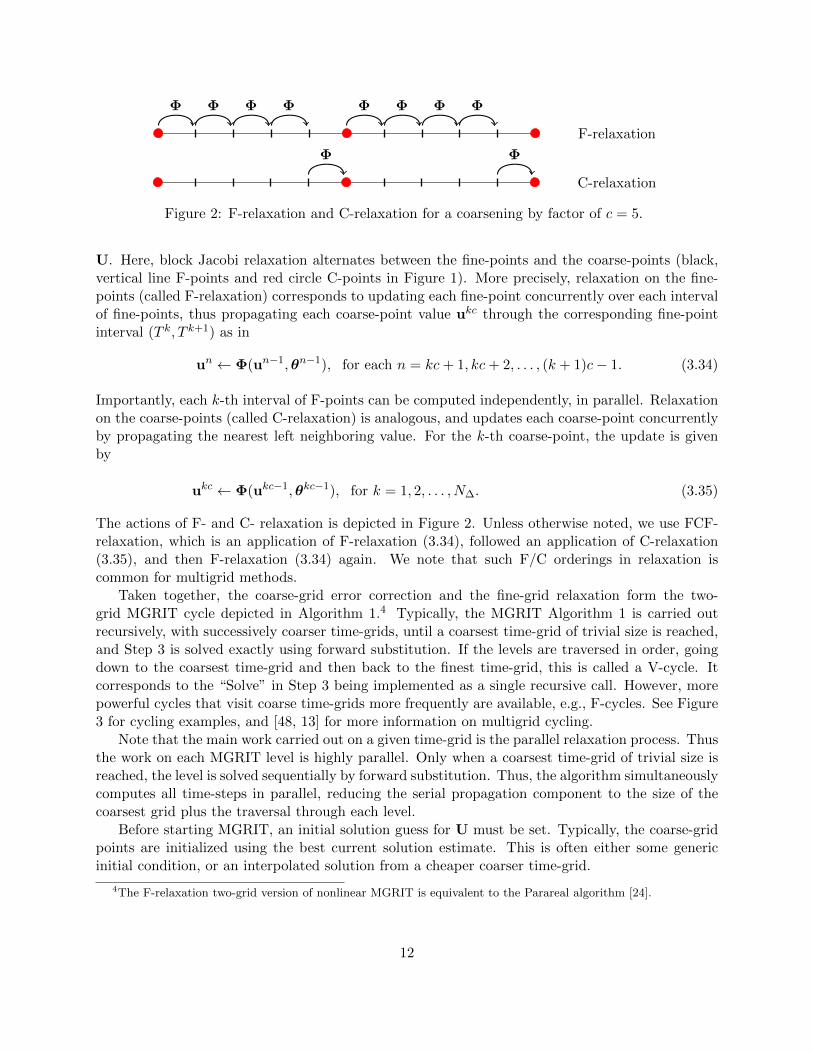
Figure 2: F-relaxation and C-relaxation for a coarsening by factor of c = 5.

U. Here, block Jacobi relaxation alternates between the fine-points and the coarse-points (black,vertical line F-points and red circle C-points in Figure 1). More precisely, relaxation on the fine-points (called F-relaxation) corresponds to updating each fine-point concurrently over each intervalof fine-points, thus propagating each coarse-point value ukc through the corresponding fine-pointinterval (T k, T k+1) as in

un ← Φ(un−1,θn−1), for each n = kc+ 1, kc+ 2, . . . , (k + 1)c− 1. (3.34)

Importantly, each k-th interval of F-points can be computed independently, in parallel. Relaxationon the coarse-points (called C-relaxation) is analogous, and updates each coarse-point concurrentlyby propagating the nearest left neighboring value. For the k-th coarse-point, the update is givenby

ukc ← Φ(ukc−1,θkc−1), for k = 1, 2, . . . , N∆. (3.35)

The actions of F- and C- relaxation is depicted in Figure 2. Unless otherwise noted, we use FCF-relaxation, which is an application of F-relaxation (3.34), followed an application of C-relaxation(3.35), and then F-relaxation (3.34) again. We note that such F/C orderings in relaxation iscommon for multigrid methods.

Taken together, the coarse-grid error correction and the fine-grid relaxation form the two-grid MGRIT cycle depicted in Algorithm 1.4 Typically, the MGRIT Algorithm 1 is carried outrecursively, with successively coarser time-grids, until a coarsest time-grid of trivial size is reached,and Step 3 is solved exactly using forward substitution. If the levels are traversed in order, goingdown to the coarsest time-grid and then back to the finest time-grid, this is called a V-cycle. Itcorresponds to the “Solve” in Step 3 being implemented as a single recursive call. However, morepowerful cycles that visit coarse time-grids more frequently are available, e.g., F-cycles. See Figure3 for cycling examples, and [48, 13] for more information on multigrid cycling.

Note that the main work carried out on a given time-grid is the parallel relaxation process. Thusthe work on each MGRIT level is highly parallel. Only when a coarsest time-grid of trivial size isreached, the level is solved sequentially by forward substitution. Thus, the algorithm simultaneouslycomputes all time-steps in parallel, reducing the serial propagation component to the size of thecoarsest grid plus the traversal through each level.

Before starting MGRIT, an initial solution guess for U must be set. Typically, the coarse-gridpoints are initialized using the best current solution estimate. This is often either some genericinitial condition, or an interpolated solution from a cheaper coarser time-grid.

4The F-relaxation two-grid version of nonlinear MGRIT is equivalent to the Parareal algorithm [24].

12

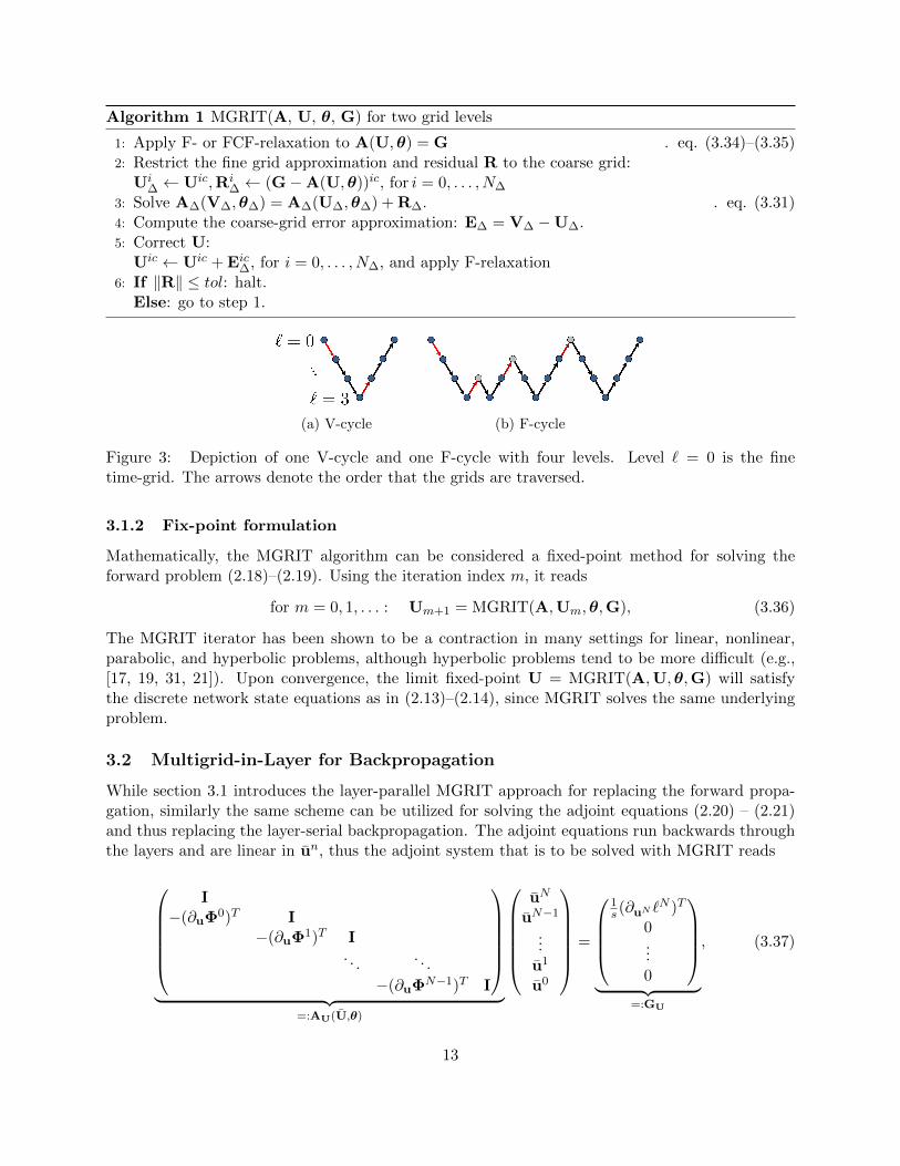
Algorithm 1 MGRIT(A, U, θ, G) for two grid levels

1: Apply F- or FCF-relaxation to A(U,θ) = G . eq. (3.34)–(3.35)2: Restrict the fine grid approximation and residual R to the coarse grid:

Ui∆ ← Uic,Ri

∆ ← (G−A(U,θ))ic, for i = 0, . . . , N∆

3: Solve A∆(V∆,θ∆) = A∆(U∆,θ∆) + R∆. . eq. (3.31)4: Compute the coarse-grid error approximation: E∆ = V∆ −U∆.5: Correct U:

Uic ← Uic + Eic∆, for i = 0, . . . , N∆, and apply F-relaxation

6: If ‖R‖ ≤ tol: halt.Else: go to step 1.

(a) V-cycle (b) F-cycle

Figure 3: Depiction of one V-cycle and one F-cycle with four levels. Level ` = 0 is the finetime-grid. The arrows denote the order that the grids are traversed.

3.1.2 Fix-point formulation

Mathematically, the MGRIT algorithm can be considered a fixed-point method for solving theforward problem (2.18)–(2.19). Using the iteration index m, it reads

for m = 0, 1, . . . : Um+1 = MGRIT(A,Um,θ,G), (3.36)

The MGRIT iterator has been shown to be a contraction in many settings for linear, nonlinear,parabolic, and hyperbolic problems, although hyperbolic problems tend to be more difficult (e.g.,[17, 19, 31, 21]). Upon convergence, the limit fixed-point U = MGRIT(A,U,θ,G) will satisfythe discrete network state equations as in (2.13)–(2.14), since MGRIT solves the same underlyingproblem.

3.2 Multigrid-in-Layer for Backpropagation

While section 3.1 introduces the layer-parallel MGRIT approach for replacing the forward propa-gation, similarly the same scheme can be utilized for solving the adjoint equations (2.20) – (2.21)and thus replacing the layer-serial backpropagation. The adjoint equations run backwards throughthe layers and are linear in un, thus the adjoint system that is to be solved with MGRIT reads

I

−(∂uΦ0)T I−(∂uΦ1)T I

. . .. . .

−(∂uΦN−1)T I

︸︷︷︸

=:AU(U,θ)

uN

uN−1

...u1

u0

=

1s (∂uN `N )T

0...0

︸︷︷︸

=:GU

, (3.37)

13

where again un denotes the adjoint variable at layer n for a general example y or for a batch ofexamples yk, k ∈ S ⊂ {1, . . . , s}. Further, (∂uΦn)T denotes the partial derivative ∂uΦ(un,θn)T .It corresponds to the backwards layer-propagation of adjoint sensitivities which in the case of aforward Euler discretization for Φ (i.e., ResNet architecture), reads

∂uΦ(un,θn)T un+1 = un+1 + h∂uF (un,θn)T un+1. (3.38)

Each backward propagator at layer n depends on the primal state un, hence the system matrixand right-hand-side of (3.37) depend on the current state U which is reflected in the subscript AU

and GU. The structure of the adjoint system (3.37), however, is the same as that of the statesystem (3.27). Hence the same MGRIT approach as presented in Algorithm 1 can be utilizedto solve the adjoint equations with the layer-parallel multigrid scheme by applying the followingiteration

Um+1 = MGRIT(AU, Um,θ,GU); (3.39)

for the adjoint vector U := (uN , . . . , u0).

3.3 Non-intrusive implementation

The MGRIT algorithm relies on the action of the layer-to-layer forward and backward propaga-tors, Φ and ∂uΦT , and their respective re-discretizations, Φ∆ and ∂uΦT

∆, on coarser grid levels.However, it does not access or “know” the internals of these functions. Hence, MGRIT can beapplied in a fully non-intrusive way with respect to any existing discretization of the nonlineardynamics describing the network forward and backward propagation. A user can wrap existingsequential evolution operators according to an MGRIT software interface, and then the MGRITcode iteratively computes the solution to (2.18)–(2.19) and (2.20)–(2.21) in parallel.

Our chosen MGRIT implementation for time-parallel computations (forwards and backwards)is XBraid [50]. One particular advantage of XBraid is its generic and flexible user-interface thatrequires relatively straight-forward user-routines which likely already exist, such as how to takeinner-products and norms with vectors un, how to take a time-step with Φ and ∂uΦT , etc. Formore details on the various user-defined functions, see the simple examples included with thepackage [50].

Since the user defines the action of Φ, any existing implementation of layer computations cancontinue to be used, including accelerator code, e.g., for GPUs. The internals of Φ are completelyopaque to XBraid. However since Φ takes a single time-step, any use of GPU kernels for Φ impliesmemory movement to and from the CPU every time-step. This is because current architectureslargely rely on the CPU to handle the message passing layer of parallelism, and it is over thislayer that XBraid provides temporal parallelism. However, future implementations could move themessage passing layer to occur solely on the GPU, thus removing this memory movement overhead.Additionally, the bandwidth and latency between CPUs and accelerators will continue to improve,also ameliorating this issue.

In [31], the XBraid library was extended with the ability to compute parallel-in-time gradientsbased on automatic differentiation (AD). The AD-based adjoint iteration solves the state andadjoint equations simultaneously with MGRIT such that gradients of the objective function arecomputed alongside the state computation.

14

4 Simultaneous Layer-Parallel Training

The state and adjoint MGRIT iterations described in Section 3 recover at convergence the samereduced gradient as a serial forward- and backpropagation through the network. They can thus beintegrated into any gradient-based training algorithm for updating the network control parametersθ,W,µ. Sub-gradient methods, such as SGD or other batch approaches can also be utilized bychoosing the subset S ⊂ {1, . . . , s} correspondingly. The layer-parallel computations are partic-ularly attractive in the small-batch mode when options for data parallelism are limited. Thus,we expect a runtime speedup over a layer-serial approach for deep networks through the greaterconcurrency within the state and adjoint solves, when the computational resources are large enough.

In order to speed up the training process even further, this section introduces a simultaneoustraining algorithm that solves the network state and adjoint inexactly during training and thusperforms network parameter updates based on inexact gradient information. We thus aim atsolving the necessary optimality conditions of the training problem in an all-at-once fashion, wherestate, adjoint and design equations are updated in a coupled iteration simultaneously.

To this end, we reduce the accuracy of the state and adjoint MGRIT solver during training andupdate the network control parameters utilizing inexact gradient information. This correspondsto an early stopping of the MGRIT iterations in each outer optimization cycle. The idea andtheoretical background of this early-stopping approach of the inner fixed-point iteration for thestate and adjoint equations is based on the One-shot method [9], which has proven successfulin reducing the computational costs for PDE-constrained optimization, mostly in aerodynamicapplications [38, 25, 8]. Here, it has been observed that the cost for a simultaneous One-shotoptimization is only a small multiple of the cost of a pure simulation of the underlying fixed-pointsolver, measured in iteration counts as well as computational runtimes. This small overhead whencompared to a reduced-space optimization will further speed up the training runtimes.

Algorithm 2 Simultaneous One-shot optimization

1: Perform m1 state updates . layer-parallel on p processorsfor m = 1, . . . ,m1 : Um ← MGRIT(A,Um−1,θ,G)

2: Perform m2 adjoint updates . layer-parallel on p processorsfor m = 1, . . . ,m2 : Um ← MGRIT(AUm1

, Um−1,θ,GUm1)

3: Assemble gradient

∇θnJ =∑

k∈S

(∂θnΦ(un

k,m1,θn)

)Tun+1k,m2

+ (∂θnR(θ,W,µ))T , ∀n = 0, . . . , N − 1

∇θinJ =

∑k∈S (∂θin

Fin(yk,θin))T u0k,m2

+ (∂θinR(θ,W,µ))T

∇WJ = 1|S|∑

k∈S

(∂W`(uN

k,m1,W,µ, ck)

)T+ (∂WR(θ,W,µ))T

∇µJ = 1|S|∑

k∈S

(∂µ`(u

Nk,m1

,W,µ, ck))T

+ (∂µR(θ,W,µ))T

4: Approximate the Hessians Bθ,BW,Bµ and select a stepsize α > 05: Network control parameter update:

θ ← θ − αB−1θ ∇θJ

W←W − αB−1W∇WJ

µ ← µ− αB−1µ ∇µJ

6: If converged: haltElse: go to step 1.

15

Algorithm 2 presents the proposed simultaneous layer-parallel One-shot training approach. Toclarify the details of the algorithm, the following points need to be considered:

• Number of state and adjoint updates m1,m2: The numbers m1,m2 ∈ N determine the numberof layer-parallel multigrid updates for the state and the adjoint variables in each optimizationcycle. If m1,m2 are large, the solutions to the state and adjoint equations are approximatedwith high accuracy in each training iteration. Hence, a conventional reduced-space trainingapproach is recovered where only the serial forward and backward propagation through thenetwork are replaced by layer-parallel MGRIT iterations. In contrast, considering smallernumbers of inner MGRIT iterations, e.g. m1,m2 ∈ {1, 2}, yields a simultaneous optimizationapproach where the network state, adjoint and control variables are updated simultaneouslyin a coupled iteration. Hence, control updates in Step 5 are based on inexact gradient infor-mation utilizing the most recent state and adjoint variables (un

m1) and (un

m2).

For the extreme case m1 = m2 = 1, the resulting optimization iteration can mathematicallybe interpreted as an approximate, reduced sequential quadratic programming (rSQP) methodwith convergence analysis presented in [38]. In [10], theoretical considerations on the choice ofm1,m2 is presented, which rely on the accuracy of the state and adjoint residual by searchingfor descent on an augmented Lagrangian function. In practice, choosing m1,m2 to be as smallas 2 has proven successful in our experience.

• Hessian approximation: In order to prove convergence of the One-shot method on a theoret-ical level, the preconditioners Bθ,BW,Bµ should approximate the Hessian of an augmentedLagrangian function that involves the residual of the state and adjoint equations (elaboratetheoretical analysis can be found in [9] and references therein). Numerically, we approximatethe Hessian through consecutive limited-memory BFGS updates based on the current reducedgradient (thus assuming that the residual term is small). Alternatively, one might try to ap-proximate the Hessian with a scaled identity matrix, which drastically reduces computationalcomplexity and has already proven successful in various applications of the One-shot methodfor aerodynamic optimization. It should be noted, that the Hessian with respect to W,µ canbe computed directly as it involves only the second derivative of the loss function ` in (2.5).

• Stepsize selection: The stepsize α is selected through a standard line-search procedure basedon the current value of the objective function, e.g. a backtracking line-search satisfying the(strong) Wolfe-condition (see, e.g., [45]).

• Stopping criterion: In Step 6 of the One-shot algorithm, a criterion for convergence andhence termination needs to be chosen. Standard optimization techniques utilize a toleranceon the norm of the gradient. In contrast, since the One-shot method targets optimality andfeasibility of the state and adjoint variables simultaneously, the stopping criterion shouldalso involve the norm of the state and adjoint residuals. In the context of network training,however, solving the optimization problem to high accuracy is often not desirable in orderto prevent training the network to match the specific input data set Y × C, i.e. overfitting.The training goal is rather to find network control parameters that generalize well on datathat has not been used for training, i.e. on a validation data set. A validation accuracy istherefore computed in each iteration of the above algorithm by applying the current networkcontrols to a separate validation dataset. We terminate the optimization algorithm, if the

16

current network controls produce a high validation accuracy, rather than focusing on thecurrent residuals of the state, adjoint and gradient norms.

The simultaneous layer-parallel training algorithm aims at reducing the runtime of conventionaltraining algorithms in two ways: First, it enables a new dimension for parallelism across the networklayers using the nonlinear multigrid approach, which goes in addition to data-parallelism across dataelements. This allows for leveraging high-performance compute clusters to speed up the trainingprocess. Second, due to the iterative nature of the layer-parallel multigrid computation, earlystopping can be applied to the state and gradient computation. Thus inexact gradient informationcan be utilized already while solving for the network state, targeting feasibility and optimalitysimultaneously.

5 Numerical Results

In this section, we investigate the computational benefits of the simultaneous layer-parallel trainingapproach on three test cases. For each test case, we first investigate runtime scaling results of thelayer-parallel MGRIT propagation for one single objective function and gradient evaluation, andcompare it to conventional serial-in-layer forward- and backpropagation (Section 5.2). Then, weintegrate the layer-parallel MGRIT iterations into the simultaneous training framework in Section5.3.

For all test cases, our focus is on the ability to achieve fast training for very deep neural networksby introducing parallelism between the layers. It is likely, though not explored here, that greatercombined speedups could be obtained by additionally using data-parallelism or parallelizing insideof each layer. Further studies are required to better understand the trade-off of distributing parallelwork between layer-parallel and data-parallel.

5.1 Test cases

1. Level set classification (Peaks example):

As a first step, we consider the test problem suggested in [32] which consists of classifyinggrid points into five level sets of the smooth nonlinear function

f(y1, y2) = 3(1− y1)2 exp(−y21 − (y2 + 1)2)− 10(y1/5− x3

1 − y52) exp(−y2

1 − y22)

−1/3 exp(−(y1 + 1)2 − y22).

The training data set consists of s = 5000 randomly chosen points yk ∈ [−3, 3]2, k = 1, . . . , s,and unit vectors ck ∈ R5 which represent the probability that a point yk belongs to level seti ∈ {1, 2, 3, 4, 5}, see Figure 4. The goal is to train a network such that it predicts the correctlevel sets for new points in [−3, 3]2 (validation points).

We choose a ResNet architecture with ReLU activation (i.e. σ(x) = max{0, x}, smoothedaround zero) and define the linear operations K(·) at each layer to be a dense matrix rep-resentation of the weights θn. We choose a network depth of T = 5 discretized with up toN = 2048 layers and a network width of 8 such that un ∈ R8, ∀n = 0, . . . , N .

2. Hyperspectral image segmentation (Indian Pines):

17

(a) True classes (b) Predicted classes

Figure 4: True and predicted level sets of the peaks function.

In this test case, we consider a soil segmentation problem based on a hyperspectral imagedata set. The input data consists of hypersectral bands over a single landscape in Indiana,US, (Indian Pines data set [3]) for 145× 145 pixels. For each pixel, the data set contains 220spectral reflectance bands which represent different portions of the electromagnetic spectrumin the wavelength range 0.4−2.5 ·10−6. The goal is to classify each pixel of the scene into oneof 16 classes (alfalfa, corn-notill, corn-mintill, corn, grass-pasture, grass-trees, grass-pasture-mowed, hay-windrowed, oats, soybean-notill, soybean-mintill, soybean-clean, wheat, woods,buildings-grass-trees-drives, stone-steel-towers). For training the network, we use the spectralbands from s = 1000 randomly chosen pixel points, yk ∈ R220, k = 1, . . . , s, together withtheir corresponding class probability vectors ck ∈ R16 (unit vectors). The goal is to predictthe correct classes of new pixel points in the scene (Figure 5).

We use a ResNet architecture with ReLU activation (i.e. σ(x) = max{0, x}, smoothed aroundzero) and define the linear operations K(·) at each layer to be a dense matrix representationof the weights θn. We choose a network depth of T = 20 discretized with up to N = 2048layers and a network width of 220 channels.

3. MNIST image classification (MNIST )

As a final example, we consider the now classic MNIST test case for classification of hand-written digits encoded in a 28 × 28 grey scale image [44]. Our objective for this test caseis to demonstrate the scalability of the layer-parallel approach over an increasing number oflayers. While we obtain reasonable validation accuracy, the objective is not to develop anoptimal ResNet to solve this problem. Further, we obtained the timings below with our ownstraight-forward implementation of convolutions, to ensure compatible layer-to-layer propa-gators with XBraid for our initial tests. Future work will use a fast convolution library, whichwill provide a substantial speedup to both the serial and layer-parallel codes.

We use a ResNet architecture with tanh activation and define internal layers by the linearoperator K(·) using 8 convolution kernels of width 3. This yields a weight tensor at each layerof size R3×3×8×8. The parameters to be trained are R28×28 at each layer. The opening layer,

18

(a) Sample band (b) True classes (c) Predicted classes

Figure 5: Indian Pines data set. Training on 1000 pixels, validation accuracy 70%.

provides a replication of the original image to the 8 convolutions with an applied activation(there are no weights in the opening layer). A final classification layer is applied that takesthe 8 convolutions using a dense K(·) to the 10 classes associated with MNIST. The internallayers are defined to have a network depth of T = 5 with up to N = 2048 layers.

For all cases, the optimization objective function consists of the softmax loss function, plus aTikhonov-regularization term for θ,W and µ, as well as an additional regularization term for θthat enforces smoothness across the network layers. The computations for the MNIST results wereperformed on the Skybridge capacity cluster at Sandia National Laboratories. Skybridge is a Craycontaining 1848 nodes with two 8 core Intel 2.6 GHz Sandy Bridge processors, 64GB of RAM pernode and an Infiniband interconnect.

5.2 Layer-parallel scaling and performance validation

First, we compare the performance of the layer-parallel MGRIT approach for forward and backwardpropagation to a layer-serial implementation. We consider one objective function and gradientevaluation for fixed network weights using a batch of examples of sizes s = 5000, 1000, 500 for thepeaks, indian pines and MNIST test case, respectively. We choose a coarsening factor of c = 4 toset up a hierarchy of ever coarser layer grids to employ the multigrid scheme.

Figure 6 shows the convergence history of the MGRIT iterations for two different problem sizesusing N = 256 and N = 1024 layers. Here, we monitor the relative drop of the state and adjointresidual norms during the MGRIT iterations. It proves fast convergence for all test cases andindependent of the number of layers.

Figure 7 presents a weak-scaling study for the layer-parallel MGRIT iterations. Here, we doublethe number of layers as well as the number of compute cores while keeping the ratio N/#cores = 4fixed, such that each compute unit processes 4 layers. Runtimes are measured for one objectivefunction and gradient evaluation with the layer-parallel MGRIT appraoch, using a relative stoppingcriterion for the MGRIT residual norms of 5 orders of magnitude. Note, that the layer-serial datapoints have been added for comparison, even though they are executed on only one core. For thelayer-serial propagation, doubling the number of layers leads to a doubling in runtime. The layer-parallel MGRIT approach however yields nearly constant runtimes independent of the problemsize. The resulting speedups are reported in Table 1. Since the layer-parallel MGRIT approach

19

10−910−810−710−610−510−410−310−210−1100101

0 1 2 3 4 5

rel.

resi

dual

iteration

N = 256 stateN = 256 adjointN = 2048 stateN = 2048 adjoint

(a) Peaks example

10−910−810−710−610−510−410−310−210−1100101

0 1 2 3 4 5

rel.

resi

dual

iteration


(b) Indian Pines

10−12

10−10

10−8

10−6

10−4

10−2

100

0 1 2 3 4

rel.

resi

dual

iteration


(c) MNIST

Figure 6: Convergence history of MGRIT solving the state and adjoint equations for N = 256 andN = 2048 layers.

20

0246810121416

256 512 1024 2048

64 128 256 512ti

me

(sec

)

# layers

# cores

Layer-parallelLayer-serial

(a) Peaks example

0

200

400

600

800

1000

1200

1400

256 512 1024 2048

64 128 256 512

tim

e(s

ec)

# layers

# cores


(b) Indian Pines

0

500

1000

1500

2000

2500

256 512 1024 2048

64 128 256 512

tim

e(s

ec)

# layers

# cores


(c) MNIST

Figure 7: Runtime comparison of a layer-parallel gradient evaluation with layer-serial forwardand backpropagation. The layer-parallel approach yields nearly constant runtimes for increasingproblem sizes and computational resources.

removes the linear runtime scale of the conventional serial-layer propagation, resulting speedupsincrease linearly with the problem size yielding up to a factor of 18x for the MNIST case using2048 layers and 512 cores. Further speedup can be expected when considering ever more layers(and computational resources).

A strong scaling study for all test cases is presented Figure 8 for various numbers of layers.Here, we keep the problem sizes fixed and measure the time-to-solution for one gradient evaluationwith MGRIT for increasing numbers of computational resources. It shows good strong scalingbehavior for all test cases, independent of the numbers of layers. The cross over point where thelayer-parallel MGRIT approach shows speedup over the layer-serial propagation is around 16 coresfor all cases (compare with the layer-serial runtimes from Table 1).

5.3 Simultaneous layer-parallel training validation

We investigate the simultaneous layer-parallel training for the Peaks and Indian Pines test cases,performing m1,m2 = 2 layer-parallel MGRIT iterations in each outer training iteration. For thePeaks example, we train a network with N = 1024 layers distributed onto 256 compute cores andfor the Indian Pines data set, we choose N = 512 layers distributed onto 128 compute cores, giving

21

Testcase N #Cores Layer-parallel Layer-serial Speedup

Peaks 256 64 1.2 sec 1.8 sec 1.8512 128 1.4 sec 3.7 sec 2.6

1024 256 1.6 sec 7.1 sec 4.92048 512 1.8 sec 13.9 sec 8.1

Indian 256 64 1.3 min 2.6 min 2.0Pines 512 128 1.5 min 5.2 min 3.3

1024 256 1.7 min 10.4 min 6.12048 512 2.0 min 20.8 min 10.3

MNIST 256 64 1.3 min 4.5 min 3.4512 128 1.9 min 9.1min 4.8

1024 256 1.7 min 18.3 min 10.52048 512 2.3 min 36.6 min 16.0

Table 1: Runtime speedup of layer-parallel gradient evaluation over layer-serial propagation.

1

2

4

8

16

2 4 8 16 32 64 128 256 512

tim

e(s

ec)

# cores

N = 256N = 512N = 1024N = 2048

(a) Peaks example

64

128

256

512

1024

2 4 8 16 32 64 128 256 512

tim

e(s

ec)

# cores

N = 256N = 512N = 1024N = 2048

(b) Indian Pines

64

128

256

512

1024

2 4 8 16 32 64 128 256 512

tim

e(s

ec)

# cores

N = 256N = 512N = 1024N = 2048

(c) MNIST

Figure 8: Strong scaling study for a layer-parallel gradient evaluation for various problem sizesfrom N = 256 to N = 2048 layers. The cross-over point where the layer-parallel approach yieldsspeedup over the layer-serial propagation lies around 16 cores (compare to Table 1).

22

4 layers per processor in both test cases. We compare runtimes of the simultaneous layer-paralleltraining with a conventional layer-serial training approach, while choosing the same precondition-ing Hessian approximation (L-BFGS), as well as the same initial network parameters for bothapproaches. However, we tune the optimization hyper-parameters (such as regularization parame-ters, stepsize selection, etc.) separately for both schemes, in order to find the best setting for eitherapproach that reaches a prescribed validation accuracy with least iteration counts and minimumruntime.

Figure 9 plots the training history for the layer-parallel simultaneous optimization approachcompared to a conventional layer-serial training approach. We validate from the top figures, thatboth approaches reach comparable performance in terms of training result (optimization iterationcounts, training loss and validation accuracy). Hence, reducing the accuracy of the inner multigriditerations for solving the state and adjoint equations within a simultaneous training frameworkdoes not deteriorate the training behavior. But, each iteration of the simultaneous layer-parallelapproach is much faster than for the layer-serial approach due to the layer-parallelization and thereduced state and adjoint accuracy. Therefore, the overall runtime for reaching that same finaltraining result is reduced drastically (bottom figures). Runtime speedups are reported in Table2. We observe a speedup of 6.0 for the Peaks example when using 256 cores, which is a parallelefficiency of about 2.3%. In the larger Indian Pines example, the reported speedup of 4.4 using 128cores gives a parallel efficiency of 3.4%. This reduces the time-to-solution from about 45 hours toabout 10 hours. While these results have been computed for selected fixed N , it is expected thatthe speedup scales linearly with increasing numbers of layers, similar to the observation in Table 1.

Test case N #Cores Layer-parallel Layer-serial Speedup

Peaks example 1024 256 683 sec 4096 sec 6.0Indian Pines 512 128 597 min 2623 min 4.4

Table 2: Runtime speedup of simultaneous layer-parallel training over layer-serial training.

6 Conclusion

In this paper, we provide a proof-of-concept for layer-parallel training of deep residual neuralnetworks (ResNets). The similarity of training ResNets to the optimal control of nonlinear time-dependent differential equations motivate us to use parallel-in-time methods that have been popularin many engineering applications. The method developed is based on nonlinear multigrid methodsand introduces a new form of parallelism across layers.

We demonstrate two options to benefit from the layer-parallel approach. First, the nonlin-ear multigrid reduction in time (MGRIT) method can be used to replace forward and backwardpropagation in existing training algorithms, including for stochastic approximation methods suchas SGD. In our experiments, this leads to speedup over serial implementations when using morethan 16 compute nodes. Second, additional savings can be obtained through the simultaneouslayer-parallel training, which uses only inexact forward and backward propagations.

While the reported speedups might seem small in terms of parallel efficiency, these reductionscan be of significant importance when considering large overall training runtimes. When baretraining runtimes are in the order of days, any runtime reduction is appreciated, as long as compu-

23

00.20.40.60.81

1.21.41.61.8

0 50 100 150 200 250 3000

20

40

60

80

100

trai

ning

loss

valid

atio

nac

cura

cy(%

)

iteration

Simultaneous layer-parallelLayer-serial reference

(a) Peaks: Training over iteration counts

00.10.20.30.40.50.60.70.80.91

0 50 100 150 200 250 300 35001020304050607080

trai

ning

loss

valid

atio

nac

cura

cy(%

)

iteration


(b) Indian Pines: Training over iteration counts

00.20.40.60.81

1.21.41.61.8

0 1000 2000 3000 40000

20

40

60

80

100

trai

ning

loss

valid

atio

nac

cura

cy(%

)

compute time (sec)


(c) Peaks: Training over time

00.10.20.30.40.50.60.70.80.91

0 5 10 15 20 25 30 35 40 4501020304050607080

trai

ning

loss

valid

atio

nac

cura

cy(%

)

compute time (hours)


(d) Indian Pines: Training over time

Figure 9: Training loss (solid lines) and validation accuracy (dashed lines) over training iterations(top) and compute time (bottom). For the layer-parallel training, each core processes 4 layers. Thesimultaneous layer-parallel approach reaches training results comparable to a layer-serial approachwithin much less computational time.

tational resources are available. Further, since training a network typically involves careful choiceof hyper-parameters, faster training runtimes will enable faster hyper-parameter optimization andthus eventually lead to better training results in general. Lastly, we mention that such efficienciesfor multigrid-in-time are not uncommon [20], where the nonintrusiveness of MGRIT contributes tothe seemingly low efficiency, as does the fact that we are defining the efficiency of MGRIT withrespect to an optimal serial algorithm. If the efficiency were defined with respect to MGRIT using1 core, then the efficiencies would be higher.

Motivated by these first promising results, we will investigate the use of layer-parallel trainingfor more challenging learning tasks, including more complex image-recognition problems. Furtherreducing the memory footprint of our algorithm in those applications motivates the use of reversiblenetworks arising from hyperbolic systems [14]. A challenge arising here is the interplay of MGRITand hyperbolic systems.

24

References

[1] M. Abadi, P. Barham, J. Chen, Z. Chen, A. Davis, J. Dean, M. Devin, S. Ghemawat, G. Irving,M. Isard, et al. Tensorflow: a system for large-scale machine learning. In OSDI, volume 16,pages 265–283, 2016.

[2] Y. S. Abu-Mostafa, M. Magdon-Ismail, and H.-T. Lin. Learning from data, volume 4. AML-Book New York, NY, USA:, 2012.

[3] M. F. Baumgardner, L. L. Biehl, and D. A. Landgrebe. 220 band aviris hyperspectral imagedata set: June 12, 1992 indian pine test site 3, Sep 2015.

[4] Y. Bengio et al. Learning deep architectures for AI. Foundations and trends R© in MachineLearning, 2(1):1–127, 2009.

[5] G. Biros and O. Ghattas. Parallel Lagrange–Newton–Krylov–Schur Methods for PDE-Constrained Optimization. Part I: The Krylov–Schur Solver. SIAM Journal on ScientificComputing, 27(2):687–713, 2005.

[6] A. Bordes, S. Chopra, and J. Weston. Question Answering with Subgraph Embeddings. arXivpreprint arXiv:1406.3676, June 2014.

[7] A. Borzı and V. Schulz. Computational optimization of systems governed by partial differentialequations. SIAM, 2011.

[8] T. Bosse, N. Gauger, A. Griewank, S. Gunther, L. Kaland, and et al. Optimal design withbounded retardation for problems with non-separable adjoints. International Series of Nu-merical Mathematics, 165:67–84, 2014.

[9] T. Bosse, N. Gauger, A. Griewank, S. Gunther, and V. Schulz. One-shot approaches to designoptimzation. International Series of Numerical Mathematics, 165:43–66, 2014.

[10] T. Bosse, L. Lehmann, and A. Griewank. Adaptive sequencing of primal, dual, and design stepsin simulation based optimization. Computational Optimization and Applications, 57(3):731–760, 2014.

[11] L. Bottou, F. Curtis, and J. Nocedal. Optimization methods for large-scale machine learning.SIAM Review, 60(2):223–311, 2018.

[12] A. Brandt. Multi–level adaptive solutions to boundary–value problems. Math. Comp.,31(138):333–390, 1977.

[13] W. L. Briggs, V. E. Henson, and S. F. McCormick. A multigrid tutorial. SIAM, Philadelphia,PA, USA, 2nd edition, 2000.

[14] B. Chang, L. Meng, E. Haber, L. Ruthotto, D. Begert, and E. Holtham. Reversible architec-tures for arbitrarily deep residual neural networks. In AAAI Conference on AI, 2018.

[15] R. Collobert, J. Weston, L. Bottou, M. Karlen, K. Kavukcuoglu, and P. Kuksa. Natu-ral Language Processing (Almost) from Scratch. Journal of Machine Learning Research,12(Aug):2493–2537, 2011.

25

[16] J. Dean, G. Corrado, R. Monga, K. Chen, M. Devin, M. Mao, A. Senior, P. Tucker, K. Yang,Q. V. Le, et al. Large scale distributed deep networks. In Advances in neural informationprocessing systems, pages 1223–1231, 2012.

[17] V. Dobrev, T. Kolev, N. Petersson, and J. Schroder. Two-level convergence theory for multi-grid reduction in time (MGRIT). Copper Mountain Special Selection, SIAM J. Sci. Comput.(accepted), 2016.

[18] W. E. A Proposal on Machine Learning via Dynamical Systems. Comm. Math. Statist.,5(1):1–11, 2017.

[19] R. D. Falgout, S. Friedhoff, T. V. Kolev, S. P. MacLachlan, and J. B. Schroder. Parallel timeintegration with multigrid. SIAM J. Sci. Comput., 36(6):C635–C661, 2014. LLNL-JRNL-645325.

[20] R. D. Falgout, S. Friedhoff, T. V. Kolev, S. P. MacLachlan, J. B. Schroder, and S. Vandewalle.Multigrid methods with space–time concurrency. Computing and Visualization in Science,18(4-5):123–143, 2017.

[21] R. D. Falgout, T. A. Manteuffel, B. O’Neill, and J. B. Schroder. Multigrid reduction intime for nonlinear parabolic problems: A case study. SIAM Journal on Scientific Computing,39(5):S298–S322, 2017.

[22] J. Friedman, T. Hastie, and R. Tibshirani. The elements of statistical learning, volume 1.Springer series in statistics Springer, Berlin, 2001.

[23] M. J. Gander. 50 years of time parallel time integration. In T. Carraro, M. Geiger, S. Korkel,and R. Rannacher, editors, Multiple Shooting and Time Domain Decomposition, pages 69–114.Springer, 2015.

[24] M. J. Gander and S. Vandewalle. Analysis of the parareal time-parallel time-integrationmethod. SIAM J. Sci. Comput., 29(2):556–578, 2007.

[25] N. Gauger and E. Ozkaya. Single-step one-shot aerodynamic shape optimization. InternationalSeries of Numerical Mathematics, 158:191–204, 2009.

[26] M. B. Giles and N. A. Pierce. An introduction to the adjoint approach to design. Flow,Turbulence and Combustion, 65(3):393–415, 2000.

[27] A. N. Gomez, M. Ren, R. Urtasun, and R. B. Grosse. The reversible residual network: Back-propagation without storing activations. In Adv Neural Inf Process Syst, pages 2211–2221,2017.

[28] I. Goodfellow, Y. Bengio, and A. Courville. Deep Learning. MIT Press, Nov. 2016.

[29] A. Griewank and A. Walther. Evaluating Derivatives: Principles and Techniques of Algorith-mic Differentiation. SIAM, 2008.

[30] S. Gunther, N. R. Gauger, and J. B. Schroder. A non-intrusive parallel-in-time adjointsolver with the XBraid library. Comput. Vis. Sci., 19:85–95, 2018. available at arXiv,math.OC/1705.00663.

26

[31] S. Gunther, N. R. Gauger, and J. B. Schroder. A non-intrusive parallel-in-time approachfor simultaneous optimization with unsteady pdes. Optimization Methods and Software (toappear), 2018. arXiv preprint arXiv:1801.06356.

[32] E. Haber and L. Ruthotto. Stable architectures for deep neural networks. Inverse Probl.,34:014004, 2017.

[33] A. Harlap, D. Narayanan, A. Phanishayee, V. Seshadri, N. Devanur, G. Ganger, and P. Gib-bons. Pipedream: Fast and efficient pipeline parallel dnn training, 2018.

[34] K. He, X. Zhang, S. Ren, and J. Sun. Deep residual learning for image recognition. InProceedings of the IEEE Conference on Computer Vision and Pattern Recognition, pages 770–778, 2016.

[35] K. He, X. Zhang, S. Ren, and J. Sun. Identity Mappings in Deep Residual Networks. InEuropean Conference on Computer Vision, pages 630–645, Mar. 2016.

[36] G. Hinton, L. Deng, D. Yu, G. E. Dahl, A.-r. Mohamed, N. Jaitly, A. Senior, V. Vanhoucke,P. Nguyen, T. N. Sainath, et al. Deep neural networks for acoustic modeling in speech recogni-tion: The shared views of four research groups. IEEE Signal Processing Magazine, 29(6):82–97,2012.

[37] F. N. Iandola, M. W. Moskewicz, K. Ashraf, and K. Keutzer. Firecaffe: near-linear accelerationof deep neural network training on compute clusters. In Proceedings of the IEEE Conferenceon Computer Vision and Pattern Recognition, pages 2592–2600, 2016.

[38] K. Ito, K. Kunisch, V. Schulz, and I. Gherman. Approximate nullspace iterations for KKTsystems. SIAM Journal on Matrix Analysis and Applications, 31(4):1835–1847, 2010.

[39] S. Jean, K. Cho, R. Memisevic, and Y. Bengio. On Using Very Large Target Vocabulary forNeural Machine Translation. arXiv preprint arXiv:1412.2007, Dec. 2014.

[40] J. Keuper and F.-J. Preundt. Distributed training of deep neural networks: Theoretical andpractical limits of parallel scalability. In Proceedings of the Workshop on Machine Learning inHigh Performance Computing Environments, pages 19–26. IEEE Press, 2016.

[41] A. Krizhevsky, I. Sutskever, and G. Hinton. Imagenet classification with deep convolutionalneural networks. Advances in neural information processing systems, 61:1097–1105, 2012.

[42] Y. LeCun, Y. Bengio, and G. Hinton. Deep learning. Nature, 521(7553):436–444, 2015.

[43] Y. LeCun, B. E. Boser, and J. S. Denker. Handwritten digit recognition with a back-propagation network. In Advances in neural information processing systems, pages 396–404,1990.

[44] Y. LeCun, L. Bottou, Y. Bengio, and P. Haffner. Gradient-based learning applied to documentrecognition. Proceedings of the IEEE, 86(11):2278–2324, 1998.

[45] J. Nocedal and S. Wright. Numerical Optimization. Springer Science+Business Media, 2ndedition, 2006.

27

[46] F. Rosenblatt. The perceptron: A probabilistic model for information storage and organizationin the brain. Psychological review, 65(6):386–408, Nov. 1958.

[47] J. B. Schroder. Parallelizing over artificial neural network training runs with multigrid. Techni-cal report, Lawrence Livermore National Laboratory, LLNL-JRNL-736173, arXiv:1708.02276,2017.

[48] U. Trottenberg, C. Oosterlee, and A. Schuller. Multigrid. Academic Press, San Diego, 2001.

[49] Q. Wang, P. Moin, and G. Iaccarino. Minimal repetition dynamic checkpointing algorithm forunsteady adjoint calculation. SIAM Journal on Scientific Computing, 31(4):2549–2567, 2009.

[50] XBraid: Parallel multigrid in time. software available at https://github.com/XBraid/

xbraid/.

[51] J. C. Ziems and S. Ulbrich. Adaptive multilevel inexact SQP methods for PDE-constrainedoptimization. SIAM Journal on Optimization, 21(1):1–40, 2011.

28

Documents

Layer-Parallel Training of Deep Residual Neural Networks