LC99, Oct. 21 - 26, 1999, Italy J. Gao, LAL, Orsay, France fileLC99, Oct. 21 - 26, 1999, Italy J. Gao, LAL, Orsay, France In tro duction T o ac hiev e the required luminosit y in a

Analytical Treatment of Single and Multibunch

Emittance Growths in Linear Colliders

Jie GAO

LAL, Orsay, France

LC99, Oct 21-26, 1999

INFN, Frascati, Italy

1

LC99, Oct. 21 - 26, 1999, Italy J. Gao, LAL, Orsay, France

Contents

� Introduction� Single bunch emittance growth

� Multi Bunch emittance growth

� Conclusions

2


Introduction

To achieve the required luminosity in a future e+e� linear collider one

has to produce two colliding beams at the interaction point (IP) with

extremely small transverse beam dimensions. According to the linear

collider design principles described in ref. 1, the normalized beam

emittance in the vertical plane (the normalized beam emittance in the

horizontal plane is larger) at IP can be expressed as:

�y =n4 re

374��B�4

(1)

where is the normalized beam energy, re = 2:82 � 10�15 m is the

classical electron radius, � = 1=137 is the �ne structure constant, ��B is

the maximum tolerable beamstrahlung energy spread, and n is the mean

number of beamstrahlung photons per electron at IP. Taking ��B = 0:03

and n = 1, one �nds �y = 8:86� 10�8mrad.

3


Single bunch emittance growth

1 Equation of transverse motion: Langevin equation

The di�erential equation of the transverse motion of a bunch with zero

transverse dimension is given as:

d2y(s; z)

ds2+

1

(s; z)

d (s; z)

ds

dy(s; z)

ds+ k(s; z)2y(s; z)

=1

m0c2 (s)e2Ne

Z1

z�(z0)W?(s; z

0 � z)y(s; z0)dz0 (2)

where k(s; z) is the instantaneous betatron wave number at position

s, z denotes the particle longitudinal position inside the bunch, andR1�1

�(z0)dz0 = 1.

Now we rewrite eq. 2 as follows:

d2y(s; z)

ds2+ �

dy(s; z)

ds+ k(s; z)2y(s; z) = � (3)

where � = (0)G (s;z)

, G = eEzm0c

2 (0), Ez is the e�ective accelerating gradient in

the linac, � = e2NeW?(s;z)y(s;0)

m0c2 (s;z)

, W?(s; z) =R1z �(z0)W?(s; z

0 � z)dz0, and

y(s; 0) is the deviation of the bunch head with respect to accelerating

structures center.

To make an analogy between the movement of the transverse motion

of an electron and that of a molecule, we de�ne P = e2NeW?(s;z)lsm0c

2 (s;z), and

regard y(s; 0)P as the particle's "velocity" random increment (�dyds)

over the distance ls, where ls is the accelerating structure length. What

4


we are interested is to assume that the random accelerating structure

misalignment error follows Gaussian distribution:

f(y(s; 0)) =1p2��y

exp

0B@�y(s; 0)

2

2�2y

1CA (4)

and the velocity (u) distribution of the molecule follows Maxwellian

distribution:

g(u) =

vuut m

2�kTexp

0B@�mu2

2kT

1CA (5)

where m is the molecule's mass, k is the Boltzmann constant, and T is

the absolute temperature. The fact that the molecule's velocity follows

Maxwellian distribution permits us to get the distribution function for

�ls:

�(�ls) =1p4�qls

exp

0B@��2l2s

4qls

1CA (6)

where

q = �kT

m(7)

By comparing eq. 6 with eq. 4, one gets:

2�2y =4qlsP 2

(8)

orkT

m=�2yP

2

2ls�(9)

Till now one can use all the analytical solutions concerning the random

motion of a molecule governed by eq. 3 by a simple substitution described

in eq. 9. Under the condition, k2(s; z) >> �2

4(adiabatic condition),By

solving Langevin equation, one gets the asymptotical values for < y2 >,

< y02 >, and < yy0 > as s!1 approximately expressed as:

< y2 >=kT

mk2(s; z)=

�2yls

2 (s; z) (0)Gk2(s; z)

0B@e

2NeW?(z)

m0c2

1CA2

(10)

5


< y02 >= k2(s; z) < y2 >=�2yls

2 (s; z) (0)G

0B@e

2NeW?(z)

m0c2

1CA2

(11)

< yy0 >= 0 (12)

Inserting eqs. 23, 11, and 12 into the de�nitions of the r.m.s. emittance

and the normalized r.m.s. emittance shown in eqs. 13 and 14:

�rms =�< y2 >< y02 > � < yy0 >2

�1=2(13)

�n;rms = (s; z)�< y2 >< y02 > � < yy0 >2

�1=2(14)

one gets

�rms =�2yls

2 (s; z) (0)Gk(s; z)

0B@e

2NeW?(z)

m0c2

1CA2

(15)

and

�n;rms =�2yls

2 (0)Gk(s; z)

0B@e

2NeW?(z)

m0c2

1CA2

(16)

The e�ects of energy dispersion within the bunch can be discussed

through (s; z), k2(s; z), and W?(z), such as BNS damping. To calculate

the emittance growth of the whole bunch one has to make an appropriate

average over the bunch, say Gaussian as assumed above, as follows:

�bunchn;rms =

R1�1

�(z0)�n;rms(z0)dz0R

1�1

�(z0)dz0(17)

To make a rough estimation one can replace �(z) by a delta function

�(z � zc), and in this case the bunch emittance can be still expressed

by eq. 16 with W?(z) replaced by W?(zc), where zc is the center of the

bunch.

2 Example

We take the single bunch emittance growth in the main linac of SBLC

for example. The short range wake�elds in the accelerating S-band

6


(a) z (m)

I (A

)

(b) z (m)

I (A

)

(c) z (m)

Wz

(V/p

C/m

)

(d) z (m)

Wr

(V/p

C/m

)

0

0.05

0.1

0.15

0.2

0.25

0.3

0.35

-0.001 0 0.0010

0.05

0.1

0.15

0.2

0.25

0.3

0.35

-0.001 0 0.001

-140

-120

-100

-80

-60

-40

-20

0

-0.001 0 0.0010

2.5

5

7.5

10

12.5

15

17.5

20

22.5

-0.001 0 0.001

Figure 1: The short range wake�elds of SBLC type structure with �z = 300 �m, and the beam iris a = 0:0133 m. (a)and (b) are the bunch current distributions. (c) is monopole the longitudinal wake�eld. (d) is the dipole transversewake�eld at r = a.

structures are obtained by using the analytical formulae and shown

in Fig. 1. In the main linac the beam is injected at 3 GeV and

accelerated to 250 GeV with an accelerating gradient of 17 MV/m. The

accelerating structure length ls =6 m, the average beta function �(s) is

about 70 m (k(s; z) = 1�(s)

for smooth focusing), the bunch population

Ne = 1:1� 1010, the bunch length �z = 300 �m, and and corresponding

dipole mode short range wake�eld W?(zc) = 338 V/pC/m2. Inserting

these parameters into eq. 16, one �nds �n;rms = 8:66� �2z . If accelerating

structure misalignment error �y = 100 �m, one gets a normalized

emittance growth of 8.66�10�8 mrad, i.e., 35% increase compared with

the designed normalized emittance of 2:5� 10�7 mrad.

7


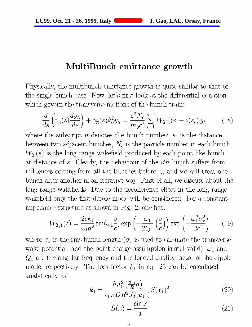
MultiBunch emittance growth

Physically, the multibunch emittance growth is quite similar to that of

the single bunch case. Now, let's �rst look at the di�erential equation

which govern the transverse motions of the bunch train:

d

ds

0@ n(s)dyn

ds

1A + n(s)k

2nyn =

e2Ne

m0c2

n�1Xi=1

WT ((n� i)sb) yi (18)

where the subscript n denotes the bunch number, sb is the distance

between two adjacent bunches, Ne is the particle number in each bunch,

WT (s) is the long range wake�eld produced by each point like bunch

at distance of s. Clearly, the behaviour of the ith bunch su�ers from

in uences coming from all the bunches before it, and we will treat one

bunch after another in an iterative way. First of all, we discuss about the

long range wake�elds. Due to the decoherence e�ect in the long range

wake�eld only the �rst dipole mode will be considered. For a constant

impedance structure as shown in Fig. 2, one has:

WT;1(s) =2ck1!1a2

sin(!1

s

c) exp

0@� !1

2Q1

sc

!1A exp0B@�!

21�

2z

2c2

1CA (19)

where �z is the rms bunch length (�z is used to calculate the transverse

wake potential, and the point charge assumption is still valid), !1 and

Q1 are the angular frequency and the loaded quality factor of the dipole

mode, respectively. The loss factor k1 in eq. 23 can be calculated

analytically as:

k1 =hJ2

1

�u11Ra�

�0�DR2J22 (u11)

S(x1)2 (20)

S(x) =sin x

x(21)

8


x1 =hu11

2R(22)

where R is the cavity radius, a is the iris radius, h is the cavity hight as

shown in Fig. 2, and u11 = 3:832 is the �rst root of the �rst order Bessel

function. To reduce the long range wake�eld one can detune and damp

the concerned dipole mode. The resultant long range wake�eld of the

detuned and damped structure (DDS) can be expressed as:

WT;DDS(s) =1

Nc

NcXi=1

2ck1;i!1;ia

2i

sin(!1;i

s

c) exp

0B@� !1;i

2Q1;i

sc

!1CA exp0B@�!

21;i�

2z

2c2

1CA

(23)

where Nc is the number of the cavities in the structure. When Nc is

very large one can use following formulae to describe ideal uniform and

Gaussian detuning structures:

1) Uniform detuning:

WT;1;U = 2 < K > sin

0@2� < f1 > s

c

1A sin(�s�f1=c)

(�s�f1=c)exp

0@�� < f1 > s

< Q >1 c

1A

(24)

2) Gaussian detuning:

WT;1;G = 2 < K > sin

0@2� < f > s

c

1A e�2(��fs=c)2 exp

0@�� < f > s

< Q >1 c

1A(25)

where K =ck1;i!1;ia

2i, f1 =

!12�, �f1 is full range the synchronous frequency

spread due to the detuning e�ect, �f is the rms width in Gaussian

frequency distribution.

Once the long range wake�eld is known one can use eq. ?? to estimate

< y2i > in an iterative way, and the emittance of the whole bunch can

be calculated accordingly as we will show later. For example, if a bunch

train is injected on axis (yn = 0) into the main linac of a linear collider

with structure rms misalignment �y, at the end of the linac one has:

< y21 >= 0 (26)

9


h

2a 2R

D

Figure 2: A disk-loaded accelerating structure.

< y22 >=(s(�2y +

<y21>

2)e2NejWT (sb)j)2(sb)ls

2 (s) (0)Gk2n(s)(m0c2)2(27)

< y23 >=

0@s(�2y +

<y21>

2)e2NejWT (2sb)j +

s(�2y +

<y22>

2)e2NejWT (sb)j

1A2 ls

2 (s) (0)Gk2n(s)(m0c2)2

(28)

and in a general way, one has:

< y2i >=

�Pi�1j=1

r(�2y +

12< y2j >)e

2NejWT ((i� j)sb)j�2ls

2 (s) (0)Gk2n(s)(m0c2)2(29)

Finally, one can use the following formula to estimate the projected

emittance of the bunch train:

�trainn;rms = (s)k(s)

Nb

NbXi=1

< y2i > (30)

where k(s) = kn(s) (since the bunch to bunch energy spread has been

ignored), and k(s) is the average over the linac.

3 Comparison with numerical simulation results

In this section we apply the analytical formulae established in section

3 to SBLC, TESLA and NLC linear collider projects where enormous

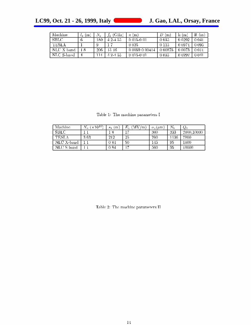
numerical simulations have been done. The machine parameters are

given in Tables 1 to 4 which have been used in the analytical calculation

in this paper. Firstly, we look at SBLC. Fig. 3 shows the \kick factor"

10


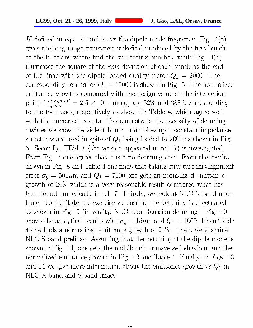
K de�ned in eqs. 24 and 25 vs the dipole mode frequency. Fig. 4(a)

gives the long range transverse wake�eld produced by the �rst bunch

at the locations where �nd the succeeding bunches, while Fig. 4(b)

illustrates the square of the rms deviation of each bunch at the end

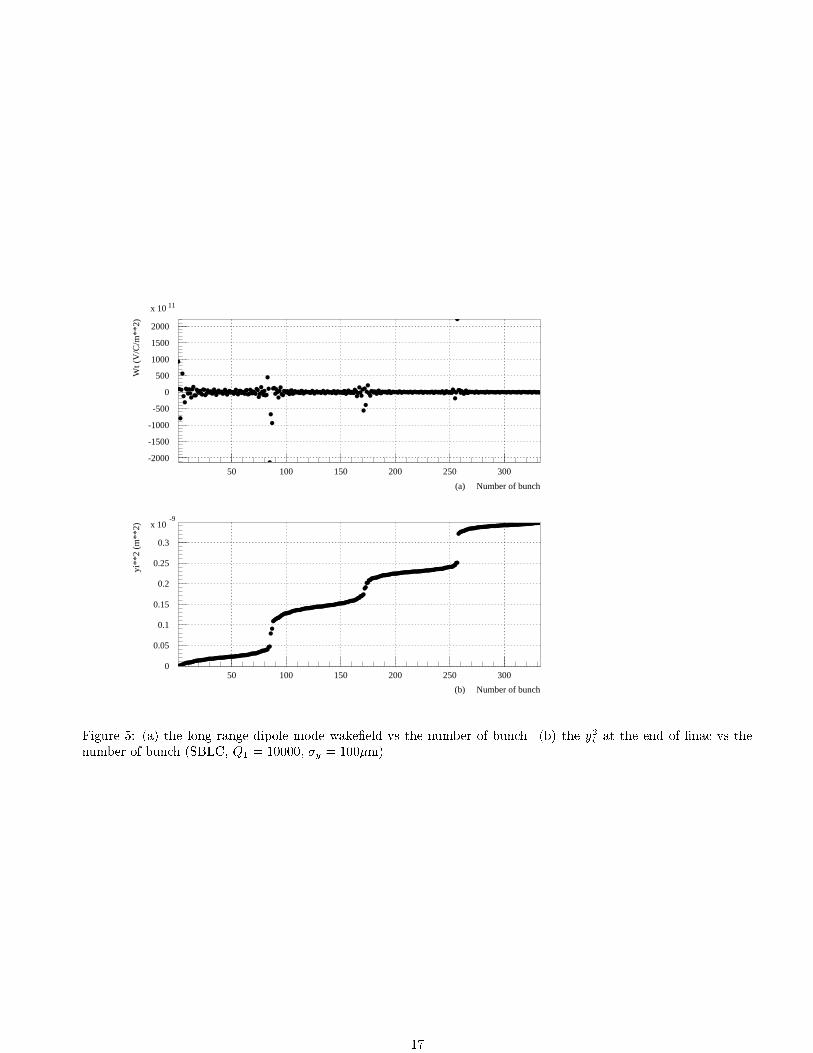
of the linac with the dipole loaded quality factor Q1 = 2000. The

corresponding results for Q1 = 10000 is shown in Fig. 5. The normalized

emittance growths compared with the design value at the interaction

point (�design;IPn;rms = 2:5 � 10�7 mrad) are 32% and 388% corresponding

to the two cases, respectively as shown in Table 4, which agree well

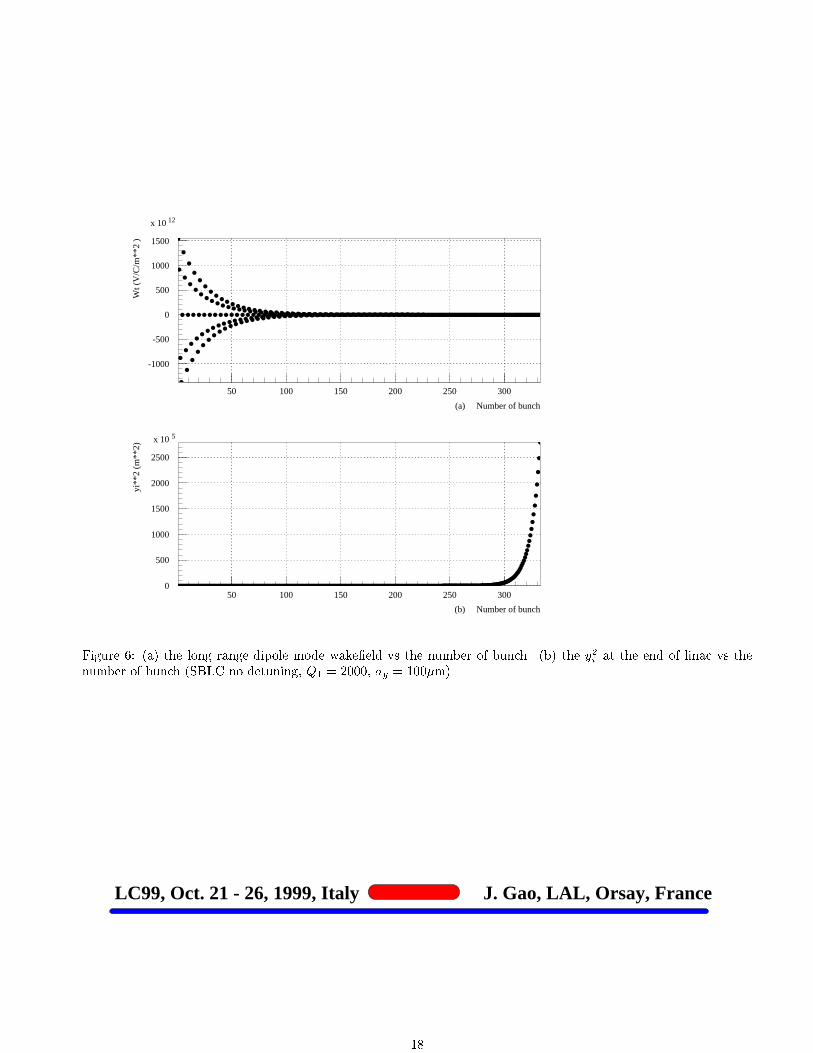
with the numerical results. To demonstrate the necessity of detuning

cavities we show the violent bunch train blow up if constant impedance

structures are used in spite of Q1 being loaded to 2000 as shown in Fig.

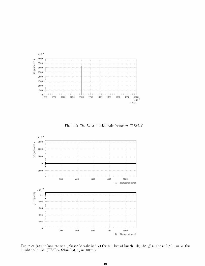
6. Secondly, TESLA (the version appeared in ref. 7) is investigated.

From Fig. 7 one agrees that it is a no detuning case. From the results

shown in Fig. 8 and Table 4 one �nds that taking structure misalignment

error �y = 500�m and Q1 = 7000 one gets an normalized emittance

growth of 24% which is a very reasonable result compared what has

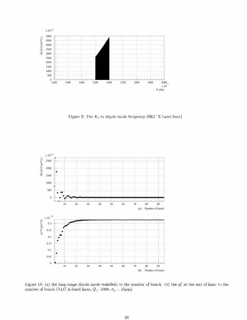
been found numerically in ref. 7. Thirdly, we look at NLC X-band main

linac. To facilitate the exercise we assume the detuning is e�ectuated

as shown in Fig. 9 (in reality, NLC uses Gaussian detuning). Fig. 10

shows the analytical results with �y = 15�m and Q1 = 1000. From Table

4 one �nds a normalized emittance growth of 21%. Then, we examine

NLC S-band prelinac. Assuming that the detuning of the dipole mode is

shown in Fig. 11, one gets the multibunch transverse behaviour and the

normalized emittance growth in Fig. 12 and Table 4. Finally, in Figs. 13

and 14 we give more information about the emittance growth vs Q1 in

NLC X-band and S-band linacs.

11


Y’

Y

Summary

Single bunch:

�n;rms =�2yls

2 (0)Gk(s; z)

0B@e

2NeW?(z)

m0c2

1CA2

(31)

�bunchn;rms =

R1�1

�(z0)�n;rms(z0)dz0R

1�1

�(z0)dz0(32)

Multibunch:

< y2i >=

�Pi�1j=1

r(�2y +

12< y2j >)e

2NejWT ((i� j)sb)j�2ls

2 (s) (0)Gk2n(s)(m0c2)2(33)

�trainn;rms = (s)k(s)

Nb

NbXi=1

< y2i > (34)

12


Conclusions

The single and multibunch emittance growths in the linacs of linear

colliders have been treated in analogy to the Brownian motions of

molecules. Analytical formulae for the emittance growth due to

accelerating structure mislaignements are established and compared with

the numerical simulation results. These formulae serve as powerful tools

parallel to the numerical ones in the optimal design of linear colliders.

13


Machine ls (m) Nc f1 (GHz) a (m) D (m) h (m) R (m)

SBLC 6 180 4.2-4.55 0.015-0.01 0.035 0.0292 0.041

TESLA 1 9 1.7 0.035 0.115 0.0974 0.095

NLC X-band 1.8 206 15-16 0.0059-0.00414 0.00875 0.0073 0.011

NLC S-band 4 114 4.2-4.55 0.015-0.01 0.035 0.0292 0.041

Table 1: The machine parameters I.

Machine Ne (�1010) sb (m) Ez (MV/m) �z(�m) Nb Q1

SBLC 1.1 1.8 17 300 333 2000,10000

TESLA 3.63 212 25 700 1136 7000

NLC X-band 1.1 0.84 50 145 95 1000

NLC S-band 1.1 0.84 17 500 95 10000

Table 2: The machine parameters II.

14


Machine (0) (GeV/MeV) (GeV/MeV) k(s) (1/m) �y (�m)

SBLC 3/0.511 250/0.511 1/90 100

TESLA 3/0.511 250/0.511 1/90 500

NLC X-band 10/0.511 250/0.511 1/50 15

NLC S-band 20/0.511 10/0.5111 1/20 50

Table 3: The machine parameters III.

Machine �train;numeri:n;rms (mrad) �train;analy:n;rms (mrad) �IP;designn;rms (mrad)

SBLC 2.3�10�8; 8:8� 10�7 8.�10�8; 9:7� 10�7 2.5�10�7

TESLA �2.5�10�8 5.9�10�8 2.5�10�7

NLC X-band - 3�10�8 1.4�10�7

NLC S-band - 1.2�10�8 1.4�10�7

Table 4: The normalized train emittance growth.

15

f (Hz)

Ki (

V/C

/m**

2)

0

200

400

600

800

1000

1200

1400

x 1012

4000 4100 4200 4300 4400 4500 4600 4700 4800 4900x 10

6

Figure 3: The Ki vs dipole mode frequency (SBLC).

(a) Number of bunch

Wt (

V/C

/m**

2)

(b) Number of bunch

yi**

2 (m

**2)

-6000

-4000

-2000

0

2000

4000

6000

8000

x 1010

50 100 150 200 250 300

0

0.02

0.04

0.06

0.08

0.1

0.12

0.14

0.16

x 10-10

50 100 150 200 250 300

Figure 4: (a) the long range dipole mode wake�eld vs the number of bunch. (b) the y2i at the end of linac vs thenumber of bunch (SBLC, Q1 = 2000, �y = 100�m).

16

(a) Number of bunch

Wt (

V/C

/m**

2)

(b) Number of bunch

yi**

2 (m

**2)

-2000

-1500

-1000

-500

0

500

1000

1500

2000

x 1011

50 100 150 200 250 300

0

0.05

0.1

0.15

0.2

0.25

0.3

x 10-9

50 100 150 200 250 300

Figure 5: (a) the long range dipole mode wake�eld vs the number of bunch. (b) the y2i at the end of linac vs thenumber of bunch (SBLC, Q1 = 10000, �y = 100�m).

17

(a) Number of bunch

Wt (

V/C

/m**

2)

(b) Number of bunch

yi**

2 (m

**2)

-1000

-500

0

500

1000

1500

x 1012

50 100 150 200 250 300

0

500

1000

1500

2000

2500

x 10 5

50 100 150 200 250 300

Figure 6: (a) the long range dipole mode wake�eld vs the number of bunch. (b) the y2i at the end of linac vs thenumber of bunch (SBLC no detuning, Q1 = 2000, �y = 100�m).


18

f1 (Hz)

Ki (

V/C

/m**

2)

0

500

1000

1500

2000

2500

3000

3500

4000

x 1010

1500 1550 1600 1650 1700 1750 1800 1850 1900 1950 2000x 10

6

Figure 7: The Ki vs dipole mode frequency (TESLA).

(a) Number of bunch

Wt (

V/C

/m**

2)

(b) Number of bunch

yi**

2 (m

**2)

-1000

0

1000

2000

3000

x 1010

200 400 600 800 1000

0

0.02

0.04

0.06

0.08

0.1

x 10-10

200 400 600 800 1000

Figure 8: (a) the long range dipole mode wake�eld vs the number of bunch. (b) the y2i at the end of linac vs thenumber of bunch (TESLA, Q1=7000, �y = 500�m).

19

f1 (Hz)

Ki (

V/C

/m**

2)

0

500

1000

1500

2000

2500

3000

3500

4000

4500

5000

x 1013

1200 1300 1400 1500 1600 1700 1800 1900 2000x 10

7

Figure 9: The Ki vs dipole mode frequency (NLC X-band linac).

(a) Number of bunch

Wt (

V/C

/m**

2)

(b) Number of bunch

yi**

2 (m

**2)

0

500

1000

1500

2000

2500

x 1012

10 20 30 40 50 60 70 80 90

0

0.05

0.1

0.15

0.2

0.25

0.3

x 10-11

10 20 30 40 50 60 70 80 90

Figure 10: (a) the long range dipole mode wake�eld vs the number of bunch. (b) the y2i at the end of linac vs thenumber of bunch (NLC X-band linac, Q1=1000, �y = 15�m).

20

f1 (Hz)

Ki (

V/C

/m**

2)

0

200

400

600

800

1000

1200

1400

x 1012

4000 4100 4200 4300 4400 4500 4600 4700 4800 4900x 10

6

Figure 11: The Ki vs dipole mode frequency (NLC S-band prelinac).

(a) Number of bunch

Wt (

V/C

/m**

2)

(b) Number of bunch

yi**

2 (m

**2)

-3000

-2000

-1000

0

1000

2000

3000

4000

x 1010

10 20 30 40 50 60 70 80 90

0

0.05

0.1

0.15

0.2

0.25

x 10-10

10 20 30 40 50 60 70 80 90

Figure 12: (a) the long range dipole mode wake�eld vs the number of bunch. (b) the y2i at the end of linac vs thenumber of bunch (NLC S-band prelinac, Q1=10000, �y = 50�m).


21

0

5 10-8

1 10-7

1.5 10-7

2 10-7

2.5 10-7

3 10-7

0 2000 4000 6000 8000 1 104

NLC X-band linac

Nor

mal

ized

em

itta

nce

(m r

ad)

Q1

Design value

Figure 13: The normalized emittance growth vs Q1 with �y = 15�m (NLC X-band linac).

0

2 10-8

4 10-8

6 10-8

8 10-8

1 10-7

1.2 10-7

1.4 10-7

0 2000 4000 6000 8000 1 104

NLC S-band prelinac

Nor

mal

ized

em

itta

nce

(m r

ad)

Q1

Design value

Figure 14: The normalized emittance growth vs Q1 with �y = 50�m (NLC S-band linac).


22

Documents

LC99, Oct. 21 - 26, 1999, Italy J. Gao, LAL, Orsay, France fileLC99, Oct. 21 - 26, 1999, Italy J. Gao, LAL, Orsay, France In tro duction T o ac hiev e the required luminosit y in a