Embed Size (px)
Citation preview

LEADING EDGE STALL
A thesis submitted to the University of Manchester
for the degree of Doctor of Philosophy
in the Faculty of Engineering and Physical Sciences
2011
Kwan Yee Chan
School of Mathematics
Contents
Abstract 15
Declaration 16
Copyright Statement 17
Acknowledgements 19
1 Introduction 20
1.1 A Brief Introduction to the Thesis . . . . . . . . . . . . . . . . . . . . 20
1.2 The Navier-Stokes Equations . . . . . . . . . . . . . . . . . . . . . . . 24
1.3 Laminar Self-Induced Separation . . . . . . . . . . . . . . . . . . . . 26
1.4 Marginal Separation . . . . . . . . . . . . . . . . . . . . . . . . . . . 31
1.5 Steady Flow on a Downstream-Moving Surface . . . . . . . . . . . . . 36
1.6 Unsteady Marginal Separation & Dynamic Stall . . . . . . . . . . . . 39
2 Boundary Layer Analysis 45
2.1 The External Inviscid Flow Region . . . . . . . . . . . . . . . . . . . 45
2.2 The Boundary Layer . . . . . . . . . . . . . . . . . . . . . . . . . . . 47
2.3 Ψ0(x, Y ) Solution . . . . . . . . . . . . . . . . . . . . . . . . . . . . . 51
2.3.1 f01(η) Solution . . . . . . . . . . . . . . . . . . . . . . . . . . 52
2.3.2 f02(η) Solution . . . . . . . . . . . . . . . . . . . . . . . . . . 53
2.3.3 Confluent Hypergeometric Functions . . . . . . . . . . . . . . 54
2.3.4 Goldstein’s Singularity . . . . . . . . . . . . . . . . . . . . . . 55
2
2.3.5 The Steady Airfoil General Solution . . . . . . . . . . . . . . . 62
2.4 Ψ1(x, Y, T ) Solution . . . . . . . . . . . . . . . . . . . . . . . . . . . . 65
2.5 Ψ0(x, Y, T ) & Ψ1(x, Y, T ) Solutions by Region . . . . . . . . . . . . . 67
2.6 Ψ2(x, Y, T ) Solution . . . . . . . . . . . . . . . . . . . . . . . . . . . . 69
2.6.1 a1(T )η Particular Solution by Frobenius Method . . . . . . . . 72
2.6.2 a2(T )η2 Particular Solution . . . . . . . . . . . . . . . . . . . 75
2.7 The Viscous Sublayer . . . . . . . . . . . . . . . . . . . . . . . . . . . 77
2.8 The Main Boundary Layer . . . . . . . . . . . . . . . . . . . . . . . . 79
3 The Interaction Region 81
3.1 Induced Pressure Gradient . . . . . . . . . . . . . . . . . . . . . . . . 83
3.2 The Middle Layer . . . . . . . . . . . . . . . . . . . . . . . . . . . . . 89
3.3 The Lower Layer . . . . . . . . . . . . . . . . . . . . . . . . . . . . . 91
3.3.1 Ψ∗1(x
∗, Y ∗, T ) Solution . . . . . . . . . . . . . . . . . . . . . . 92
3.3.2 Ψ∗2(x
∗, Y ∗, T ) Solution & the A1(x∗, T ) Function . . . . . . . . 93
3.3.3 The Fourier Transformation Boundary Value Problem . . . . . 95
3.3.4 Bessel Functions of the First Kind . . . . . . . . . . . . . . . . 99
3.3.5 General Solution . . . . . . . . . . . . . . . . . . . . . . . . . 100
3.3.6 The A(x, T ) Solvability Condition from Inverse Fourier Trans-
formation . . . . . . . . . . . . . . . . . . . . . . . . . . . . . 101
3.4 The Upper Layer . . . . . . . . . . . . . . . . . . . . . . . . . . . . . 107
4 A(x, T ) Solvability Condition Analysis 109
4.1 A(x, T ) Equation Numerical Treatment . . . . . . . . . . . . . . . . . 112
4.2 Newton’s Method for a System of Nonlinear Equations . . . . . . . . 121
4.3 Smith & Elliott (1985) Algorithm Test . . . . . . . . . . . . . . . . . 125
4.4 A(x, T ) Algorithm Test . . . . . . . . . . . . . . . . . . . . . . . . . . 143
4.4.1 The Initial Conditions . . . . . . . . . . . . . . . . . . . . . . 144
4.5 Solutions Close To The Critical Angle . . . . . . . . . . . . . . . . . . 157
4.5.1 Streamlines & Velocities . . . . . . . . . . . . . . . . . . . . . 165
3
4.5.2 Singularity & Skin Friction . . . . . . . . . . . . . . . . . . . . 172
5 The Nonlinear Breakdown 174
5.1 The Quasi-Steady Second Interactive Stage . . . . . . . . . . . . . . . 175
5.1.1 Second Interactive Flow Configuration . . . . . . . . . . . . . 180
5.1.2 The Boundary Conditions for A(X) . . . . . . . . . . . . . . . 185
5.1.3 A(X) Boundary Eigenvalue β Problem . . . . . . . . . . . . . 186
5.2 A(X) Equation Numerical Treatment . . . . . . . . . . . . . . . . . . 188
5.2.1 The Minimising Function Φ , Eigenvalue β & Boundary Value
Constant λ2 . . . . . . . . . . . . . . . . . . . . . . . . . . . . 195
5.2.2 Numerical Shooting Method . . . . . . . . . . . . . . . . . . . 196
5.2.3 Discontinuous A(x, T ) & A(X) Analysis . . . . . . . . . . . . 198
5.2.4 Newton’s Method with Minimising Function Φ . . . . . . . . . 205
5.3 A(X) Algorithm Test . . . . . . . . . . . . . . . . . . . . . . . . . . . 208
5.3.1 Numerical Shooting Method Test . . . . . . . . . . . . . . . . 209
5.3.2 Newton’s Method Test . . . . . . . . . . . . . . . . . . . . . . 217
5.3.3 The Initial Conditions . . . . . . . . . . . . . . . . . . . . . . 217
5.3.4 Comparison of the Shooting Method & Newton’s Method with Φ231
5.4 Second Interactive Stage Solutions . . . . . . . . . . . . . . . . . . . . 236
6 Leading Edge Stall 241
6.1 The Unsteady Boundary Layer . . . . . . . . . . . . . . . . . . . . . 241
6.2 The Interaction Region . . . . . . . . . . . . . . . . . . . . . . . . . . 244
6.3 An Unsteady Interactive Structure . . . . . . . . . . . . . . . . . . . 245
6.4 The Finite-Time Breakdown Problem . . . . . . . . . . . . . . . . . . 248
7 Summary & Conclusions 252
7.1 Boundary Layer Analysis & the Interaction Region . . . . . . . . . . 253
7.2 A(x,T) Solvability Condition Analysis & the Nonlinear Breakdown . . 258
7.3 Leading Edge Stall & Inviscid Euler Structure . . . . . . . . . . . . . 269
4
7.4 Further Work . . . . . . . . . . . . . . . . . . . . . . . . . . . . . . . 270
Bibliography 272
A Derivation of the Navier-Stokes Equations 280
B The Integral of Small Perturbation Theory 283
Word count: 69399
5
List of Tables
4.1 Grids and step sizes for implementing the Smith & Elliott (1985) test
in either domain x ∈ [−20, 20] or x ∈ [−40, 40]. . . . . . . . . . . . . . 126
4.2 Errors E from IC0, IC1 and IC2; domain x ∈ [−40, 40]; grid 2; at
T1000 = 0.999 to calculate A(x, T ) at T1001 = 1.0 . . . . . . . . . . . . 128
4.3 Errors E from IC3; domain x ∈ [−40, 40]; grid 2; at T1 = 0 to calculate
A(x, T ) at T2 = 0.001 and at T495 = 0.496 to calculate A(x, T ) at
Tend = 0.497. . . . . . . . . . . . . . . . . . . . . . . . . . . . . . . . . 128
4.4 Initial condition IC3 end time points Tend, by domain and grid. . . . . 128
4.5 Grids and step sizes for implementing the A(x, T ) algorithm test in
domain x ∈ [−40, 40]. . . . . . . . . . . . . . . . . . . . . . . . . . . . 144
4.6 Initial condition end times Tend, by grid. . . . . . . . . . . . . . . . . 146
4.7 Errors E from IC0, IC1, IC2 and IC3; grid 2; at T1 = 0 to calculate
A(x, T ) at T2 = 0.001. . . . . . . . . . . . . . . . . . . . . . . . . . . 147
4.8 Errors E from IC0, IC1; grid 2; at Tend − DT to calculate A(x, T ) at
Tend. . . . . . . . . . . . . . . . . . . . . . . . . . . . . . . . . . . . . 147
4.9 Errors E from IC2, IC3; grid 2; at Tend − DT to calculate A(x, T ) at
Tend. . . . . . . . . . . . . . . . . . . . . . . . . . . . . . . . . . . . . 148
4.10 Initial condition end times Tend, by grids; repeated from Table 4.6. . . 158
5.1 The second interactive stage test domains in X and grid step sizes DX .208
6
5.2 Numerical shooting method: Minimising function Φ; eigenvalue β and
boundary condition constant λ2 (both written to 4 significant figures),
by step size DX and domain. . . . . . . . . . . . . . . . . . . . . . . 210
5.3 Smith & Elliott (1985) step size DX and eigenvalue β results, for initial
distribution IC01. . . . . . . . . . . . . . . . . . . . . . . . . . . . . . 218
5.4 Newton’s method without Φ: Errors E from IC00; β(0) = β(1) = 1.20;
domain X ∈ [−50, 50]; and step size DX = 0.4. . . . . . . . . . . . . 219
5.5 Newton’s method with Φ: Errors E from IC00; β(0) = 1.20; domain
X ∈ [−50, 50]; step size DX = 0.4. . . . . . . . . . . . . . . . . . . . 220
5.6 Newton’s method with Φ: Errors E from IC00; β(0) = 1.22; domain
X ∈ [−250, 250]; step size DX = 0.05. . . . . . . . . . . . . . . . . . . 220
5.7 Newton’s method with Φ: Eigenvalue β(k) and boundary value con-
stant λ(k)2 at iterations k from IC00; domain X ∈ [−50, 50]; step size
DX = 0.4. . . . . . . . . . . . . . . . . . . . . . . . . . . . . . . . . . 221
5.8 Newton’s method with Φ: Eigenvalue β and boundary value constant
λ2 (written to 4 significant figures) from IC00, by domain and step size
DX . . . . . . . . . . . . . . . . . . . . . . . . . . . . . . . . . . . . . 222
5.9 Newton’s method with Φ: Minimising function Φ from IC00; domain
X ∈ [−50, 50]; step size DX = 0.05. . . . . . . . . . . . . . . . . . . . 228
5.10 Shooting method (S) and Newton’s method with Φ (N): Eigenvalue β
and boundary value constant λ2 (written to 4 significant figures), by
step size DX and domain. . . . . . . . . . . . . . . . . . . . . . . . . 231
7
List of Figures
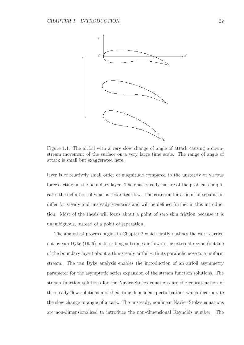
1.1 The airfoil with a very slow change of angle of attack causing a down-
stream movement of the surface on a very large time scale. The range
of angle of attack is small but exaggerated here. . . . . . . . . . . . . 22
1.2 Goldstein’s main boundary layer 2 and viscous sublayer 3 of combined
thickness O(Re12 ) about a point of separation xs = 0. The external
inviscid flow 1 has velocity Ue(x). . . . . . . . . . . . . . . . . . . . . 29
1.3 The triple-deck interaction region for steady subsonic flow: I, II, III;
viscous sublayer: 3, 3’; external inviscid region: 1; main boundary
layer: 2, 2’. There is a bubble about the point of separation xs = 0. . 31
1.4 The flow around an airfoil at angle of attack α with a short bubble, a
long bubble, and an extended separation zone (from top to bottom).
There is a stagnation point at O. . . . . . . . . . . . . . . . . . . . . 33
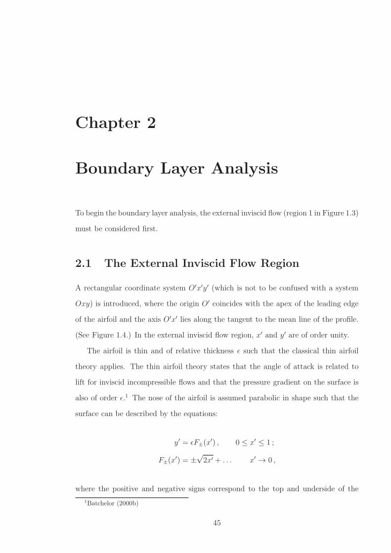
2.1 The parabolic nose of the airfoil with Cartesian coordinate system
O′X ′Y ′ for the leading edge; and orthogonal curvilinear coordinate
system Oxy for the boundary layer. . . . . . . . . . . . . . . . . . . . 46
2.2 The flow structure consists of the external inviscid region 1; the viscous
sublayers: 3 and 3’, upstream and downstream of the point of zero skin
friction x = 0; and the main boundary layers: 2 and 2’. . . . . . . . . 55
2.3 The hierarchical matching process to find solutions for the main bound-
ary layer 2 and viscous sublayer 3 upstream of the point of zero skin
friction, and the analogous regions 2’ and 3’ downstream. . . . . . . . 58
8
2.4 The triple-deck interaction region: I, II, III; viscous sublayer: 3, 3’;
external inviscid region: 1; main boundary layer: 2, 2’. . . . . . . . . 61
2.5 The flow structure consists of the external inviscid region 1; the viscous
sublayers: 3 and 3’, upstream and downstream of the point of zero skin
friction x = 0; and the main boundary layers: 2 and 2’. . . . . . . . . 69
3.1 Asymptotic structure of characteristic flow regions: the external in-
viscid region 1; main boundary layer 2; viscous sublayer 3, near a
stationary body contour AOB with small turning angle θ0. . . . . . . 83
3.2 The triple-deck interaction region: I, II, III; viscous sublayer: 3, 3’;
external inviscid region: 1; main boundary layer: 2, 2’. . . . . . . . . 87
3.3 The hierarchical matching procedure to find stream functions series
expansions for boundary layers and interaction regions. . . . . . . . . 88
3.4 Contour integration on the k-plane. . . . . . . . . . . . . . . . . . . . 103
4.1 The airfoil angle of attack law (4.3): a(T ) = 1.331 − 1.332e−T , for
T = [0, 6]. . . . . . . . . . . . . . . . . . . . . . . . . . . . . . . . . . 111
4.2 The uniform space x and time T grid, where the points x1 and xm+1 are
the start and end of the computational domain. An example integral
with some integrand [] for i = 1: I2, at x = 2 and time level T2, is shown.114
4.3 The contour in the complex plane for the integralx1∫
−∞
∂A∂T
(ξ, T ) dξ
(xi+1−ξ)14. 118
4.4 The schematic for Newton’s method to solve f(x) = 0. . . . . . . . . 122
4.5 Boundary condition BC andA(x, T ) from IC0, at T = 0.0, 0.1, . . . , 1.0,
by domain and grid. . . . . . . . . . . . . . . . . . . . . . . . . . . . 130
4.6 Boundary condition BC and A(x, T ) from IC1. See Figure 4.5. . . . . 130
4.7 Boundary condition BC and A(x, T ) from IC2. See Figure 4.5. . . . . 131
4.8 Boundary condition BC and A(x, T ) from IC3, at sample time levels
at intervals of ∆T = 0.1 until Tend, by domain and grid. . . . . . . . . 131
4.9 Boundary condition BC and A(x, T ) from IC0 at T = 0.0, 0.1, . . . , 1.0,
by domain and grid. . . . . . . . . . . . . . . . . . . . . . . . . . . . 132
9
4.10 A(x, T ) from IC1 at T = 0.6, by domain and grid. . . . . . . . . . . . 133
4.11 Smith & Elliott (1985) Figure 1(a), p. 8; A(x, T ) from initial condition
1 at T = 0.6; and from initial condition 2 at T = 0.9; also with
boundary condition A = (X2 + 1)12 , where X = x. . . . . . . . . . . . 133
4.12 A(x, T ) from IC2 at T = 0.9, by domain and grid. . . . . . . . . . . . 134
4.13 A(x, T ) from IC2, grid 2 at T = 0.9. . . . . . . . . . . . . . . . . . . . 135
4.14 Smith & Elliott (1985); see Figure 4.11. . . . . . . . . . . . . . . . . . 135
4.15 A(x, T ) from IC3 at T = 0.1, by domain and grid. . . . . . . . . . . . 136
4.16 A(x, T ) from IC3 at T = 0.2, by domain and grid. . . . . . . . . . . . 137
4.17 A(x, T ) from IC3 at T = 0.3, by domain and grid. . . . . . . . . . . . 137
4.18 A(x, T ) from IC3, grid 2 at T = 0.1, 0, 2, 0.3. . . . . . . . . . . . . . 138
4.19 Smith & Elliott (1985) Figure 1(b), p. 8; A(x, T ) from initial condition
3 at T = 0.0, 0.1, 0.2, 0.3. . . . . . . . . . . . . . . . . . . . . . . . . 138
4.20 A(x, T ) from IC3 at T = 0.45, by domain and grid. . . . . . . . . . . 140
4.21 A(x, T ) from IC3, grid 1 at T = 0.45. . . . . . . . . . . . . . . . . . . 141
4.22 Smith & Elliott (1985) Figure 1(c), p. 9; A(x, T ) from initial conditions
3 at T = 0.45. . . . . . . . . . . . . . . . . . . . . . . . . . . . . . . . 142
4.23 Boundary condition BC and A(x, T ) from IC0 at T = 0.0, 0.5, . . . , 5.0,
by grid, for domain x ∈ [−40, 40]. . . . . . . . . . . . . . . . . . . . . 149
4.24 Boundary condition BC and A(x, T ) from IC1. See Figure 4.23. . . . 150
4.25 Boundary condition BC and A(x, T ) from IC2. See Figure 4.23. . . . 150
4.26 Boundary condition BC and A(x, T ) from IC3 at T = 0.0, 0.1, . . . , 0.7,
by grid, for domain x ∈ [−40, 40]. . . . . . . . . . . . . . . . . . . . . 151
4.27 A(x, T ) from IC0 at T = 0.0, 1.0, . . . , 5.0, by grid, for domain x ∈
[−40, 40]. . . . . . . . . . . . . . . . . . . . . . . . . . . . . . . . . . . 152
4.28 A(x, T ) from IC1 at T = 0.0, 1.0, . . . , 5.0, by grid. . . . . . . . . . . . 153
4.29 A(x, T ) from IC2 at T = 0.0, 1.0, . . . , 5.0, by grid. . . . . . . . . . . . 153
4.30 A(x, T ) from IC3 at T = 0.0, 0.2, 0.4, 0.6, by grid. . . . . . . . . . . . 154
4.31 A(x, T ) from IC0 at T = 0.0, 0.5, . . . , 4.0. . . . . . . . . . . . . . . . 159
10
4.32 A(x, T ) from IC0 at T = 4.0, 4.5, 5.0 . . . . . . . . . . . . . . . . . . 159
4.33 A(x, T ) from IC1 at T = 0.0, 0.2, . . . , 1.0. . . . . . . . . . . . . . . . 160
4.34 A(x, T ) from IC1 at T = 1.2, 1.4, . . . , 2.0. . . . . . . . . . . . . . . . 160
4.35 A(x, T ) from IC1 at T = 2.5, 3.0, . . . , 5.0. . . . . . . . . . . . . . . . 161
4.36 A(x, T ) from IC2 at T = 0.0, 0.5, . . . , 3.0. . . . . . . . . . . . . . . . 163
4.37 A(x, T ) from IC2 at T = 3.0, 3.5, . . . , 5.0. . . . . . . . . . . . . . . . 163
4.38 A(x, T ) from IC3 at T = 0.0, 0.1, . . . , 0.5. . . . . . . . . . . . . . . . 164
4.39 A(x, T ) from IC3 at T = 0.5, 0.6, 0.7. . . . . . . . . . . . . . . . . . . 164
4.40 Streamlines Ψ(x, Y, T ) and tangential velocity u(x, Y, T ) from IC1 at
T = 0.0; at increments of ∆Ψ = ∆u = 2.0; starting from Ψ = u = 2.0. 166
4.41 Ψ(x, Y, T ) and u(x, Y, T ) from IC1 at T = 1.0. See Figure 4.40. . . . . 167
4.42 Ψ(x, Y, T ) and u(x, Y, T ) from IC1 at T = 2.0. See Figure 4.40. . . . . 168
4.43 Ψ(x, Y, T ) and u(x, Y, T ) from IC1 at T = 3.0. See Figure 4.40. . . . . 169
4.44 Ψ(x, Y, T ) and u(x, Y, T ) from IC1 at T = 4.0. See Figure 4.40. . . . . 170
4.45 Ψ(x, Y, T ) and u(x, Y, T ) from IC1 at T = 5.0. See Figure 4.40. . . . . 171
5.1 The point of zero skin friction x = xs and flow structure travelling
towards the point of singularity x = XS, when β ≥ α > 0. . . . . . . 177
5.2 A discontinuous A(x, T ) wave for amplitude parameter C = 1 at T =
0.0, 0.2, . . . , 1.0. . . . . . . . . . . . . . . . . . . . . . . . . . . . . . 204
5.3 A discontinuous A(x, T ) wave for C = 1 at T = 0.0 then T =
1.0, 2.0, . . . , 6.0. . . . . . . . . . . . . . . . . . . . . . . . . . . . . . 204
5.4 Numerical shooting method: Eigenvalue β versus minimising function
Φ for step sizes DX = 0.05, 0.1, by domain. . . . . . . . . . . . . . . 211
5.5 Numerical shooting method: Eigenvalue β versus step size DX , by
domain. . . . . . . . . . . . . . . . . . . . . . . . . . . . . . . . . . . 211
5.6 Numerical shooting method: Boundary condition constant λ2 versus
step size DX , by domain. . . . . . . . . . . . . . . . . . . . . . . . . 212
11
5.7 Numerical shooting method: A(X) for domain X ∈ [−50, 50], by step
size DX . . . . . . . . . . . . . . . . . . . . . . . . . . . . . . . . . . . 213
5.8 Numerical shooting method: A(X) for X ∈ [−100, 100], by step size
DX . . . . . . . . . . . . . . . . . . . . . . . . . . . . . . . . . . . . . 214
5.9 Numerical shooting method: A(X) for X ∈ [−150, 150], by step size
DX . . . . . . . . . . . . . . . . . . . . . . . . . . . . . . . . . . . . . 214
5.10 Numerical shooting method: A(X) for X ∈ [−200, 200], by step size
DX . . . . . . . . . . . . . . . . . . . . . . . . . . . . . . . . . . . . . 215
5.11 Numerical shooting method: A(X) for X ∈ [−250, 250], by step size
DX . . . . . . . . . . . . . . . . . . . . . . . . . . . . . . . . . . . . . 215
5.12 Numerical shooting method: A(X) and boundary condition BC (5.63)
for step size DX = 0.05, boundary condition constant λ2 = 0.96 and
eigenvalue β = 1.227, by domain. . . . . . . . . . . . . . . . . . . . . 216
5.13 Newton’s method with Φ: Eigenvalue β versus step size DX from IC00,
by domain. . . . . . . . . . . . . . . . . . . . . . . . . . . . . . . . . 223
5.14 Newton’s method with Φ: Boundary value constant λ2 versus step size
DX from IC00, by domain. . . . . . . . . . . . . . . . . . . . . . . . . 223
5.15 Newton’s method with Φ: A(X) for IC00; domain X ∈ [−50, 50];
step sizes DX = 0.40, 0.20, 0.10, 0.05 and respective eigenvalues β =
1.207, 1.216, 1.223, 1.226. . . . . . . . . . . . . . . . . . . . . . . . . 224
5.16 Newton’s method with Φ: A(X) for IC00; X ∈ [−100, 100]; DX =
0.40, 0.20, 0.10, 0.05 and respective β = 1.207, 1.216, 1.223, 1.226. . . 225
5.17 Newton’s method with Φ: A(X) for IC00; X ∈ [−150, 150]; DX =
0.40, 0.20, 0.10, 0.05 and respective β = 1.206, 1.216, 1.223, 1.226. . . 225
5.18 Newton’s method with Φ: A(X) for IC00; X ∈ [−200, 200]; DX =
0.40, 0.20, 0.10, 0.05 and respective β = 1.206, 1.216, 1.223, 1.226. . . 226
5.19 Newton’s method with Φ: A(X) for IC00; X ∈ [−250, 250]; DX =
0.40, 0.20, 0.10, 0.05 and respective β = 1.206, 1.216, 1.223, 1.226. . . 226
12
5.20 Newton’s method with Φ A(X) and boundary condition BC (5.63)
from IC00; step size DX = 0.05; and eigenvalue β = 1.226, by domain. 227
5.21 Newton’s method with Φ: Functions A(X) for IC01; X ∈ [−50, 50];
DX = 0.4, 0.2, 0.1, 0.05 and respective β(0) = 1.20, 1.21, 1.22, 1, 22. . 228
5.22 Newton’s method with Φ: Functions A(X) for IC01; X ∈ [−50, 50];
DX = 0.4, 0.2, 0.1, 0.05 and respective β(0) = 0.45, 0.51, 0.55, 0.58. . 229
5.23 Newton’s method with Φ: Functions A(X)(1000) for IC1; X ∈ [−50, 50];
DX = 0.4, 0.2, 0.1, 0.05 and respective β(0) = 1.20, 1.21, 1.22, 1, 22. . 230
5.24 Eigenvalue β versus step size DX by shooting method (S) and New-
ton’s method with Φ (N) from IC00, by domain. . . . . . . . . . . . . 232
5.25 Boundary value constant λ2 versus eigenvalue β by shooting method
(S) and Newton’s method with Φ (N) from IC00, by domain. . . . . . 232
5.26 A(X) by shooting method (S) and Newton’s method with Φ (N) from
IC00; X ∈ [−50, 50], by step size DX and eigenvalue β. . . . . . . . . 233
5.27 A(X) by shooting method (S) and Newton’s method with Φ (N) from
IC00; X ∈ [−100, 100], by step size DX and eigenvalue β. . . . . . . . 234
5.28 A(X) by shooting method (S) and Newton’s method with Φ (N) from
IC00; X ∈ [−150, 150], by step size DX and eigenvalue β. . . . . . . . 234
5.29 A(X) by shooting method (S) and Newton’s method (N) from IC00;
X ∈ [−200, 200], by step size DX and eigenvalue β. . . . . . . . . . . 235
5.30 A(X) by shooting method (S) and Newton’s method with Φ (N) from
IC00; X ∈ [−250, 250], by step size DX and eigenvalue β. . . . . . . . 235
5.31 Smith & Elliott (1985), Figure 3, p. 18: “Numerical solutions... show-
ing the shock-like (abrupt reattachment) trend near the origin.” . . . 236
5.32 The point of zero skin friction x = xs and flow structure travelling
towards the point of singularity x = XS, when 0 < α ≤ 1.23. . . . . . 237
5.33 A(X) for domain X ∈ [−250, 250], step size DX = 0.05; eigenvalue
β = 1.226; boundary value constant λ2 = 0.96, as shown in regions
X ∈ [−250, 250] and X ∈ [−25, 25]. . . . . . . . . . . . . . . . . . . . 239
13
5.33 A(X), as shown in region X ∈ [−2.5, 2.5]. See Figures 7.7a and 7.7b. 240
7.1 The airfoil with a very slow change of angle of attack causing a down-
stream movement of the surface on a very large time scale. The range
of angle of attack is small but exaggerated here. . . . . . . . . . . . . 253
7.2 The triple-deck interaction region: I, II, III; viscous sublayer: 3, 3’;
external inviscid region: 1; main boundary layer: 2, 2’. . . . . . . . . 255
7.3 A(x, T ) from IC1 at T = 0.0, 0.2, . . . , 1.0. . . . . . . . . . . . . . . . 260
7.4 A(x, T ) from IC1 at T = 1.2, 1.4, . . . , 2.0. . . . . . . . . . . . . . . . 261
7.5 A(x, T ) from IC1 at T = 2.5, 3.0, . . . , 5.0. . . . . . . . . . . . . . . . 261
7.6 The point of zero skin friction x = xs and flow structure travelling
towards the point of singularity x = XS, when β ≥ α > 0. . . . . . . 263
7.7 A(X) for domain X ∈ [−250, 250], step size DX = 0.05; eigenvalue
β = 1.226; boundary value constant λ2 = 0.96, as shown in regions
X ∈ [−250, 250] and X ∈ [−25, 25]. . . . . . . . . . . . . . . . . . . . 266
7.7 A(X), as shown in region X ∈ [−2.5, 2.5]. See Figures 5.33a and 5.33b. 267
7.8 Smith & Elliott (1985), Figure 3, p. 18: “Numerical solutions... show-
ing the shock-like (abrupt reattachment) trend near the origin.” . . . 268
14
The University of Manchester
Kwan Yee ChanDoctor of PhilosophyLeading Edge StallSeptember 8, 2011
An airfoil is placed in a high Reynolds number but subsonic fluid flow and issubject to very slow perturbations of its angle of attack compared to the time scaleof the flow. Asymptotic solutions for the Navier-Stokes equations are obtained forthe boundary layer and interaction region flow structure on the airfoil. The viscous-inviscid interaction between the boundary layer and external inviscid flow is on a timescale sufficiently large such that the induced pressure gradient from the displacementof the boundary layer from the surface is negligible. Numerical solutions are found forthe solvability condition from the method of matched asymptotic expansions, whichensures flow structure consistency. A short bubble of reversed recirculating flow formson the surface of the airfoil. As time progresses, the angle of attack approaches acritical angle for a skin friction singularity and nonlinear breakdown. Discontinuousskin friction solutions are obtained for a second interactive stage equation. An erup-tion process from the bubble thickens the boundary layer and terminates the secondinteractive stage, resulting in a vortex, or eddy, spanning the boundary layer. Theejection of the vortex from the surface is the process of leading edge stall.
15

Declaration
No portion of the work referred to in this thesis has been
submitted in support of an application for another degree
or qualification of this or any other university or other
institute of learning.
16

Copyright Statement
i. The author of this thesis (including any appendices and/or schedules to this
thesis) owns certain copyright or related rights in it (the “Copyright”) and s/he
has given The University of Manchester certain rights to use such Copyright,
including for administrative purposes.
ii. Copies of this thesis, either in full or in extracts and whether in hard or elec-
tronic copy, may be made only in accordance with the Copyright, Designs and
Patents Act 1988 (as amended) and regulations issued under it or, where appro-
priate, in accordance with licensing agreements which the University has from
time to time. This page must form part of any such copies made.
iii. The ownership of certain Copyright, patents, designs, trade marks and other
intellectual property (the “Intellectual Property”) and any reproductions of
copyright works in the thesis, for example graphs and tables (“Reproductions”),
which may be described in this thesis, may not be owned by the author and may
be owned by third parties. Such Intellectual Property and Reproductions can-
not and must not be made available for use without the prior written permission
of the owner(s) of the relevant Intellectual Property and/or Reproductions.
iv. Further information on the conditions under which disclosure, publication and
commercialisation of this thesis, the Copyright and any Intellectual Property
and/or Reproductions described in it may take place is available in the Univer-
sity IP Policy (see http://www.campus.manchester.ac.uk/medialibrary/
policies/intellectual-property.pdf), in any relevant Thesis restriction
17

declarations deposited in the University Library, The University Librarys regu-
lations (see http://www.manchester.ac.uk/library/aboutus/regulations)
and in The Universitys policy on presentation of Theses.
18

Acknowledgements
Thank you:
Prof. Jitesh S. B. Gajjar
Prof. Anatoly I. Ruban
The University of Manchester
Engineering and Physical Sciences Research Council
Dr Dmitry Yumashev
My mother & my father
P. A. V.
19
Chapter 1
Introduction
Flow separation from the surface of a solid body and the flow that develops as a
result of this separation is an intriguing and complex phenomenon of fluid dynamics.
Its occurrence is known to be potentially dangerous. Detached fluid flow from the
surface of an airfoil limits its lift force and can lead to stalling during flight.1 Hence,
understanding the theoretical basis and properties of flow separation, and predicting
whether it will occur or not, is desirable.
1.1 A Brief Introduction to the Thesis
High speed and low viscosity fluid flow separation from a surface of a solid body, like
all phenomenon of fluid dynamics, is governed by the Navier-Stokes equations. A
historical account follows of the introduction of the boundary layer and the methods
used to find solutions to the equations.
The introduction of the Prandtl (1904) boundary layer and the Prandtl (1935)
hierarchical principal of constructing asymptotic expansion solutions leads to the
Goldstein (1948) singularity; self-induced separation, in which there is an induced
pressure gradient by the displacement effect of the boundary layer; the triple-deck
1See Jones (1933), Jones (1934) and Tani (1964).
20
CHAPTER 1. INTRODUCTION 21
interaction region structure about a point of zero skin friction on the surface; viscous-
inviscid interaction between the boundary layer and the external part of the flow; and
bubbles of reversed recirculating flow.
In application to flight, the solid body is a thin airfoil. The angle of attack of the
airfoil, its range of values and its rate of change are important factors because they
affect the pitch, roll and yaw of an aircraft. The range of angle of attack is assumed
small. If the angle of attack of the airfoil is such that the fluid is attached to its
surface then the angle can be incrementally increased so that the steady attached
flow is forced to gradually detach from the surface. The resulting flow separation
is called marginal separation. A solvability condition resulting from the method
of matched asymptotic expansions between the regions of the triple-deck must be
satisfied for the flow structure to be consistent.
Marginal separation can be extended to quasi-steady and unsteady flows where the
angle of attack is increasing with time such that steady flow is now over a downstream-
moving surface. (See Figure 1.1.) The solvability condition is an unsteady, nonlinear,
partial integro-differential equation which relates skin (surface) friction on the airfoil
to the angle of attack. It requires numerical solution and several types of flow config-
uration are described depending on the far away boundary conditions and the initial
distribution. After a finite time, a critical limit of angle of attack is reached where
a nonlinear breakdown singularity occurs, leading to Smith (1982a) dynamic stall on
the leading edge of the airfoil.
The thesis aims to bridge the work on marginal separation with that on steady
flow over a downstream-moving surface, unsteady marginal separation and dynamic
stall. In particular, the focus is on the quasi-steady flow structure which develops
over a very large time scale when there are very slow perturbations to the otherwise
steady stream functions. The slow perturbations are from a slow change in angle of
attack over a small range as it gradually approaches the critical angle where stream
function solutions become complex and nonlinear breakdown occurs. The time scale
is sufficiently large such that the induced pressure gradient by the displaced boundary
CHAPTER 1. INTRODUCTION 22
y’
O’ x’T
Figure 1.1: The airfoil with a very slow change of angle of attack causing a down-stream movement of the surface on a very large time scale. The range of angle ofattack is small but exaggerated here.
layer is of relatively small order of magnitude compared to the unsteady or viscous
forces acting on the boundary layer. The quasi-steady nature of the problem compli-
cates the definition of what is separated flow. The criterion for a point of separation
differ for steady and unsteady scenarios and will be defined further in this introduc-
tion. Most of the thesis will focus about a point of zero skin friction because it is
unambiguous, instead of a point of separation.
The analytical process begins in Chapter 2 which firstly outlines the work carried
out by van Dyke (1956) in describing subsonic air flow in the external region (outside
of the boundary layer) about a thin steady airfoil with its parabolic nose to a uniform
stream. The van Dyke analysis enables the introduction of an airfoil asymmetry
parameter for the asymptotic series expansion of the stream function solutions. The
stream function solutions for the Navier-Stokes equations are the concatenation of
the steady flow solutions and their time-dependent perturbations which incorporate
the slow change in angle of attack. The unsteady, nonlinear Navier-Stokes equations
are non-dimensionalised to introduce the non-dimensional Reynolds number. The
CHAPTER 1. INTRODUCTION 23
Reynolds number is the ratio of the orders of magnitude of inertial and viscous forces.
The flow in the boundary layer is then characterised by a limit process of when the
Reynolds number tends to infinity.
Substituting the asymptotic expansion of the stream function into the Navier-
Stokes equations, the triple-deck regions about the point of zero skin friction can be
constructed by the hierarchical process. Boundary value problems are derived for
each term of the stream function for say, the viscous sublayer of the boundary layer.
The solutions lead to a stream function series expansion for the main boundary layer
by the method of matched asymptotic expansions.
The analysis fails when either attempts to match the boundary layer solutions
upstream of the point of zero skin friction with those downstream come to a con-
tradiction as in Goldstein’s singularity, or when the perturbations in the asymptotic
expansions becomes the same order of magnitude as the steady flow and hence are
no longer negligible. There is another region about the point of zero skin friction
with a new limit process. The interaction region is introduced in Chapter 3 and the
same hierarchical process in Chapter 2 is used to determine stream function solutions
there. The stream function solutions and triple-deck structure are consistent by the
method of matched asymptotic expansions if a solvability condition is satisfied.
Chapter 4 is on the construction of the initial-boundary value problem for the
solvability condition and its numerical solution, based on the methods set out by
Smith & Elliott (1985). Several types of initial flow configuration, from the Smith &
Elliott attached flow steady state solution to a bubble of reversed flow, lead to un-
bounded growth in skin friction after some finite time. With the numerical solutions,
stream function and velocity contours can be found. Analytical solutions are difficult
if not impossible to find.
Chapter 5 follows from the evidence of a skin friction singularity and is the analysis
as the nonlinear breakdown is approached. The unbounded skin friction can be
modelled as a discontinuous wave in the fluid. The discontinuous wave is theorised to
travel along the surface in a second interactive region. Depending on the travelling
CHAPTER 1. INTRODUCTION 24
speed of the wave, the triple-deck structure either remains intact and moves with the
point of zero skin friction, or is destroyed. A boundary value problem is solved to
describe the flow there.
Descriptions of the numerical algorithms for the solvability condition problem,
the algorithms for the second interactive stage problem, and their tests are given
in Sections 4.3, 4.4 and 5.3. The tests are for satisfaction of boundary conditions;
convergence; domain and grid size independence.
Chapter 6 describes the end of the second interactive stage based on the Elliott
& Smith (1987) dynamic stall. As the angle of attack increases, the flow continues to
develop with time. After a finite time, the second interactive stage transforms into
a third interactive stage where a vortex spans the boundary layer and is eventually
ejected. The third interactive stage is beyond the scope of the thesis since it is
characteristic of fully unsteady flow.
Summaries and conclusions from the boundary layer analysis (Chapter 2) to the
leading edge stall (Chapter 6) are given in Chapter 7.
1.2 The Navier-Stokes Equations
The Navier-Stokes equations are derived in Appendix A. The Navier-Stokes equations
for incompressible, Newtonian fluids, in the two-dimensional Cartesian coordinate
system (x, y) with time t, are:
∂u
∂t+ u
∂u
∂x+ v
∂u
∂y= fx −
1
ρ
∂p
∂x+ ν
(
∂2u
∂x2+∂2u
∂y2
)
,
∂v
∂t+ u
∂v
∂x+ v
∂v
∂y= fy −
1
ρ
∂p
∂y+ ν
(
∂2v
∂x2+∂2v
∂y2
)
,
∂u
∂x+∂v
∂y= 0 .
The variables are the tangential and normal velocity components u and v; body
forces fx, fy; pressure p; density ρ; constant kinetic viscosity ν = µ
ρ; and constant
CHAPTER 1. INTRODUCTION 25
dynamic viscosity µ. Each of the terms of the equations represent the forces of the
fluid dynamics system. Using the first, x-momentum equation as an example, the
unsteady forces are represented by the term ∂u∂t; the inertial forces by u∂u
∂x+v ∂u
∂y; body
forces by fx; pressure forces by 1ρ
∂p
∂x; and viscous forces by ν
(
∂2u∂x2 +
∂2u∂y2
)
.
For simplicity, the body forces fx and fy in the airfoil problem, such as gravity,
are neglected. The governing equations of the airfoil problem are:
∂u
∂t+ u
∂u
∂x+ v
∂u
∂y= ν
(
∂2u
∂x2+∂2u
∂y2
)
− 1
ρ
∂p
∂x,
∂v
∂t+ u
∂v
∂x+ v
∂v
∂y= ν
(
∂2v
∂x2+∂2v
∂y2
)
− 1
ρ
∂p
∂y,
∂u
∂x+∂v
∂y= 0 .
The equations may be non-dimensionalised using the variables: x = Lx, y = Ly,
t = LU∞
t, u = U∞u, v = U∞v, p = ρU2∞p, where L is the length of the airfoil chord
and U∞ is the unperturbed flow speed far away from the airfoil at infinity. The
non-dimensionalised equations (after removing the tilde notation) are:
∂u
∂t+ u
∂u
∂x+ v
∂u
∂y=
1
Re
(
∂2u
∂x2+∂2u
∂y2
)
− ∂p
∂x, (1.1)
∂v
∂t+ u
∂v
∂x+ v
∂v
∂y=
1
Re
(
∂2v
∂x2+∂2v
∂y2
)
− ∂p
∂y, (1.2)
∂u
∂x+∂v
∂y= 0 . (1.3)
The Reynolds number
Re =U∞L
ν,
is the remaining parameter. Flow at high Reynolds number concerns most natural
gas and liquid flows where there is relatively small kinetic viscosity ν compared to
unperturbed speed U∞ or length scale L. Mathematically, it is a ratio of the orders
of magnitude of inertial and viscous forces. Where fluid flow is of high speed and low
CHAPTER 1. INTRODUCTION 26
viscosity, the limit as Re→∞ is taken.
By the mass continuity equation (1.3), the velocity components u, v are written
in terms of the stream function ψ where
u =∂ψ
∂y, v = −∂ψ
∂x. (1.4)
The Navier-Stokes equations (1.1), (1.2) and (1.3) and the required two boundary
conditions and one initial condition is the basic set of equations of which the solution
describes fluid flow. There are some exact analytical solutions2 but where there is
none, the problem can be solved using the hierarchical boundary layer theory intro-
duced in the twentieth century, and the principle of matched asymptotic expansion
solutions.
1.3 Laminar Self-Induced Separation
A history of fluid dynamics in relation to flight has been written by Anderson (1997)
and Anderson (2008) and an introduction to the asymptotic solution of the Navier-
Stokes equations is presented by Sychev, Ruban, Sychev & Korolev (1998a).
In the early twentieth century, Prandtl (1904) proposed the concept of the laminar
boundary layer (as opposed to turbulent flow) to describe separation of high Reynolds
number fluid flow from the surface of solid body. Prandtl theorised that the effects
of surface skin friction are experienced only in a thin viscous boundary layer near the
surface and that the fluid particles adjacent to the surface adhered to it.3 Outside the
boundary layer, the external flow is essentially inviscid. If the type of external flow
promotes an adverse positive pressure gradient in the direction of flow then the result
is flow separation. The fluid particles with their kinetic energy dissipated in a region
where the pressure is increasing are lifted off the surface at a point of separation
2See for example, Poiseuille flow through a circular pipe, as discussed in Batchelor (2000a).3Details on the development of the boundary layer with an aerodynamic background and with
regards to vorticity is given by Lighthill (1963).
CHAPTER 1. INTRODUCTION 27
x = xs where skin friction has been driven to zero. The point of zero skin friction
coincides with the point of separation for steady cases. This is the Prandtl criterion
for flow separation.
Taking the limit as Re → ∞ results in a very small viscosity coefficient of the
highest order derivative of the Navier-Stokes equations (1.1), (1.2) such that the Euler
system of equations:
∂u
∂t+ u
∂u
∂x+ v
∂u
∂y= −∂p
∂x,
∂v
∂t+ u
∂v
∂x+ v
∂v
∂y= −∂p
∂y
are obtained (for negligible body forces fx and fy). Hence, the two boundary condi-
tions required for the equations cannot both be satisfied and so, the problem becomes
singular. The Euler equations do not account for frictional, viscous effects and so ap-
ply to the external flow. Prandtl’s boundary layer allows for viscous forces and so
the Navier-Stokes equations apply there. Nevertheless, Prandtl’s theory does not ac-
count for flow beyond the point of separation because of the adverse pressure gradient
ahead of it.
A solution to the Navier-Stokes equations was proposed by Goldstein (1930) for
steady, incompressible fluid flow in the boundary layer upstream of the point of
separation x = xs, where x < xs is considered the upstream region before separation
takes place and x > xs is considered the downstream region. The solutions for
velocity and pressure are asymptotic series expansions and are formulated assuming
there is a constant adverse pressure gradient in a finite neighbourhood of the point of
separation. Prandtl (1935) goes on to show the hierarchical principal of constructing
asymptotic expansions according to the external flow and the boundary layer regions,
and the iterative procedure of building the regions alternately whilst refining the
solutions term by term.4
Goldstein (1948), knowing the work by Landau & Lifshitz (1944), carried out a
rigorous analysis of the boundary layer close to the point of separation (which for
4See van Dyke (1975) for example.
CHAPTER 1. INTRODUCTION 28
convenience is chosen as the origin of coordinates xs = 0) and immediately ahead of it
using the method of matched asymptotic expansions. There is unbounded growth of
the transverse velocity component v inversely proportional to |∆x| 12 = |x−xs|12 whilst
the pressure gradient ratio ∆p
∆xis inversely proportional to (∆x)
13 . Numerical analysis
by Howarth (1938) and Hartree (1939) indicated singular behaviour of the solution
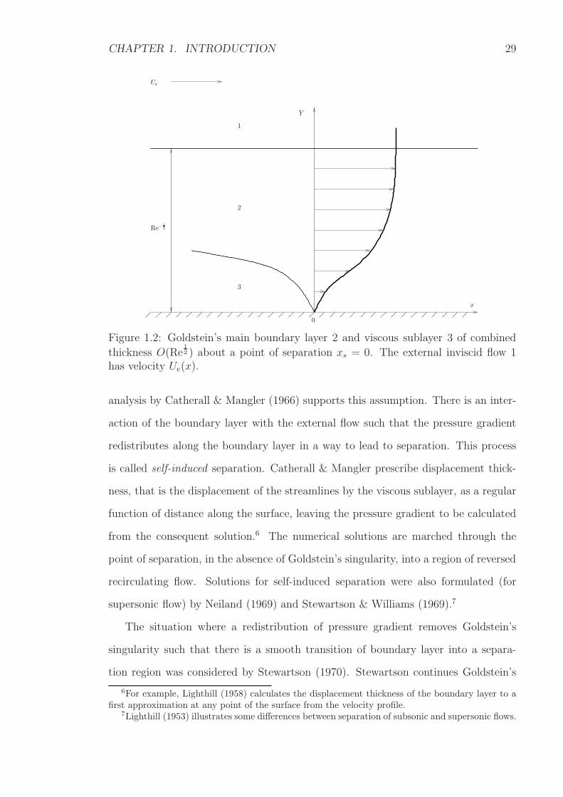
at the point of separation. Goldstein found that the boundary layer immediately
upstream of the point of separation is in fact divided into a main boundary layer
(region 2 in Figure 1.2) and a viscous sublayer (region 3) adjacent to the surface. The
viscous sublayer ensures the fluid velocity is dissipated to zero on the surface whilst
decreasing in thickness according to the rule Y → (−x) 14 as x → −0. However, the
viscous sublayer stream function solution grows exponentially as its normal coordinate
Y → ∞. The viscous sublayer solution cannot match the external region solution,
hence there is a main boundary layer in between.
Goldstein showed that the solutions cannot be constructed past the point of sepa-
ration. There is a contradiction in the terms of the asymptotic expansions as x→ +0
which results in the downstream solution for the viscous sublayer being imaginary.
Beyond the point of separation, it would seem the boundary layer ceases to exist be-
cause of the prescribed adverse pressure gradient and in the wake, the entire Navier-
Stokes equations come into action. Goldstein’s singularity implies that Prandtl’s
boundary layer hypothesis is not valid in the vicinity of the point of separation and
so cannot be a complete account of the flow structure.5 Indeed, Lighthill (1951)
renders a uniformly valid fluid speed on the aerofoil (with leading edge of radius
of curvature ρL) surface but only if a part singular like x−1 is subtracted and the
remainder is multiplied by
[
x
(x+ 12ρL)
]
.
Logarithmic term and singular term modifications were introduced into Gold-
stein’s asymptotic expansions by Stewartson (1958) and Messiter & Enlow (1973).
Each term is singular at the point of separation and it is suggested that the boundary
layer must somehow adjust itself so that these terms cannot appear. The numerical
5The evidence of Goldstein’s singularity is expanded upon in Section 2.3.4.
CHAPTER 1. INTRODUCTION 29
1
2
3
0
Re−12
Ue
Y
x
Figure 1.2: Goldstein’s main boundary layer 2 and viscous sublayer 3 of combined
thickness O(Re12 ) about a point of separation xs = 0. The external inviscid flow 1
has velocity Ue(x).
analysis by Catherall & Mangler (1966) supports this assumption. There is an inter-
action of the boundary layer with the external flow such that the pressure gradient
redistributes along the boundary layer in a way to lead to separation. This process
is called self-induced separation. Catherall & Mangler prescribe displacement thick-
ness, that is the displacement of the streamlines by the viscous sublayer, as a regular
function of distance along the surface, leaving the pressure gradient to be calculated
from the consequent solution.6 The numerical solutions are marched through the
point of separation, in the absence of Goldstein’s singularity, into a region of reversed
recirculating flow. Solutions for self-induced separation were also formulated (for
supersonic flow) by Neiland (1969) and Stewartson & Williams (1969).7
The situation where a redistribution of pressure gradient removes Goldstein’s
singularity such that there is a smooth transition of boundary layer into a separa-
tion region was considered by Stewartson (1970). Stewartson continues Goldstein’s
6For example, Lighthill (1958) calculates the displacement thickness of the boundary layer to afirst approximation at any point of the surface from the velocity profile.
7Lighthill (1953) illustrates some differences between separation of subsonic and supersonic flows.
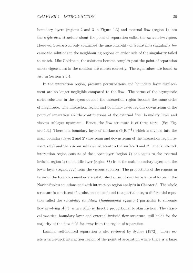
CHAPTER 1. INTRODUCTION 30
boundary layers (regions 2 and 3 in Figure 1.3) and external flow (region 1) into
the triple-deck structure about the point of separation called the interaction region.
However, Stewartson only confirmed the unavoidability of Goldstein’s singularity be-
cause the solutions in the neighbouring regions on either side of the singularity failed
to match. Like Goldstein, the solutions become complex past the point of separation
unless eigenvalues in the solution are chosen correctly. The eigenvalues are found in
situ in Section 2.3.4.
In the interaction region, pressure perturbations and boundary layer displace-
ment are no longer negligible compared to the flow. The terms of the asymptotic
series solutions in the layers outside the interaction region become the same order
of magnitude. The interaction region and boundary layer regions downstream of the
point of separation are the continuations of the external flow, boundary layer and
viscous sublayer upstream. Hence, the flow structure is of three tiers. (See Fig-
ure 1.3.) There is a boundary layer of thickness O(Re−12 ) which is divided into the
main boundary layer 2 and 2′ (upstream and downstream of the interaction region re-
spectively) and the viscous sublayer adjacent to the surface 3 and 3′. The triple-deck
interaction region consists of the upper layer (region I) analogous to the external
inviscid region 1; the middle layer (region II) from the main boundary layer; and the
lower layer (region III) from the viscous sublayer. The proportions of the regions in
terms of the Reynolds number are established in situ from the balance of forces in the
Navier-Stokes equations and with interaction region analysis in Chapter 3. The whole
structure is consistent if a solution can be found to a partial integro-differential equa-
tion called the solvability condition (fundamental equation) particular to subsonic
flow involving A(x), where A(x) is directly proportional to skin friction. The classi-
cal two-tier, boundary layer and external inviscid flow structure, still holds for the
majority of the flow field far away from the region of separation.
Laminar self-induced separation is also reviewed by Sychev (1972). There ex-
ists a triple-deck interaction region of the point of separation where there is a large
CHAPTER 1. INTRODUCTION 31
1
2
2’
3’
0
3
II
I
III
y
x
Re−12
Figure 1.3: The triple-deck interaction region for steady subsonic flow: I, II, III;viscous sublayer: 3, 3’; external inviscid region: 1; main boundary layer: 2, 2’. Thereis a bubble about the point of separation xs = 0.
self-induced pressure gradient. The fluid velocity being relatively slow in the vis-
cous sublayer compared to the rest of the boundary layer is sensitive to pressure
fluctuations. Any deceleration of fluid particles from an adverse pressure gradient
causes the sublayer to become thicker such that streamlines are displaced from the
surface. The displacement, or the slope of the streamlines, is transmitted through
the main boundary layer to the external flow where the pressure perturbations feed-
back to the viscous sublayer to induce more displacement. The feedback is termed
viscous-inviscid interaction and continues until the perturbations are so large that
the streamline detaches from the wall. Upon detachment, a region of reversed recir-
culating flow is formed called the separation bubble. When the bubble erupts, there
is a wake downstream of the point of separation.
1.4 Marginal Separation
Marginal separation at the leading edge of a thin airfoil is reviewed by Sychev, Ruban,
Sychev & Korolev (1998b).
CHAPTER 1. INTRODUCTION 32
Goldstein’s singularity is associated with strong boundary layer separation and
its strength can be reduced by varying a parameter controlling the adverse pressure
gradient acting on the layer. The parameter is the angle of attack (angle of incidence)
of a slender airfoil with a parabolic leading edge.8 When the attached flow on the
airfoil is forced to gradually approach separation by increasing the angle of attack
then the eventual detachment is called marginal separation.
In experimental observations,9 the air flow around the airfoil is attached to the
surface when the angle of attack is small and below a critical value. When the angle
of attack is above the critical value (but within a small range), there is the formation
of a closed region of recirculating flow, a so-called “short bubble”. The length of the
bubble does not usually exceed 1% of the airfoil chord and its presence has little effect
upon the aerodynamic forces acting on the airfoil. With increase in angle of attack,
the bubble eventually bursts to form either a so-called “long bubble” or a stagnation
zone. (See Figure 1.4.) Accompanying the change in flow field is a decrease in lift
and an increase in drag acting on the airfoil. In the application of flight, a sudden
increase in drag acting on an airfoil performing a relatively slow oscillation through
a large angle past the critical angle of attack can lead to stalling.10
Werle & Davis (1972) detail a numerical solution to the boundary layer problem
consisting of Prandtl’s classical equation (for the boundary layer normal coordinate
Y ):11
∂Ψ
∂Y
∂2Ψ
∂x∂Y− ∂Ψ
∂x
∂2Ψ
∂Y 2=∂3Ψ
∂Y 3− ∂pe∂x
;
the no-slip condition; a matching condition with the external inviscid region; an initial
condition at the flow stagnation point O; and Bernoulli’s equation for the external
8Stewartson, Smith & Kaups (1982) and Smith & Elliott (1985) respectively define a slender
airfoil as having a thickness ratio less than Re−1
16 or a thickness to chord ratio comparable to asufficiently small angle of attack.
9See for example, the review by Tani (1964).10See Crabtree (1959) and Smith (1982a).11A quasi-steady version of Prandtl’s classical equation (2.14) is derived later from the Navier-
Stokes equation (1.1) and streamfunction (1.4) in Chapter 2.
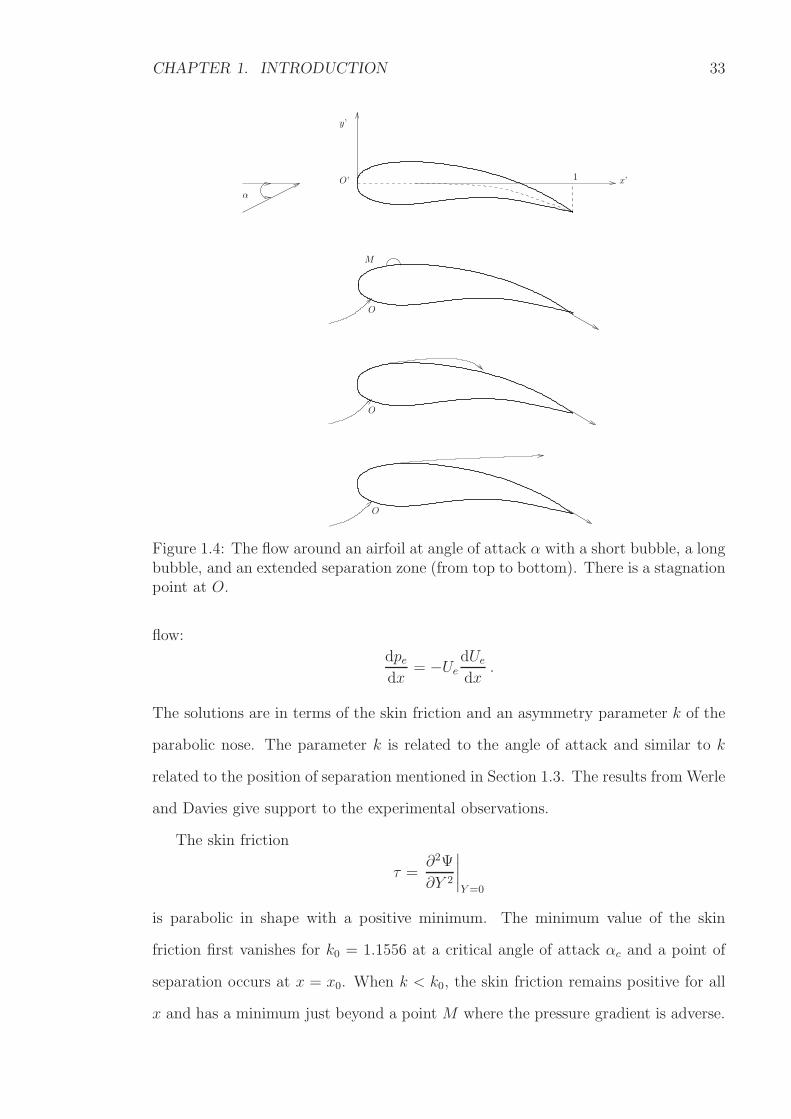
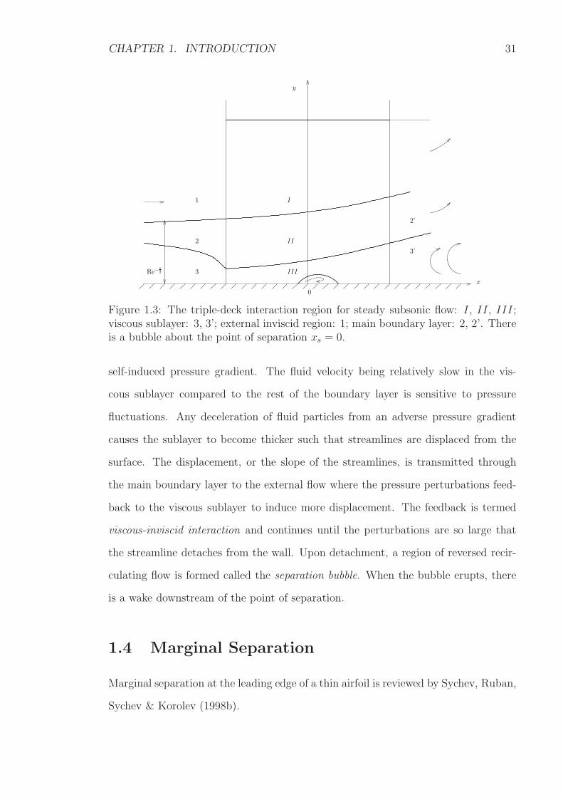
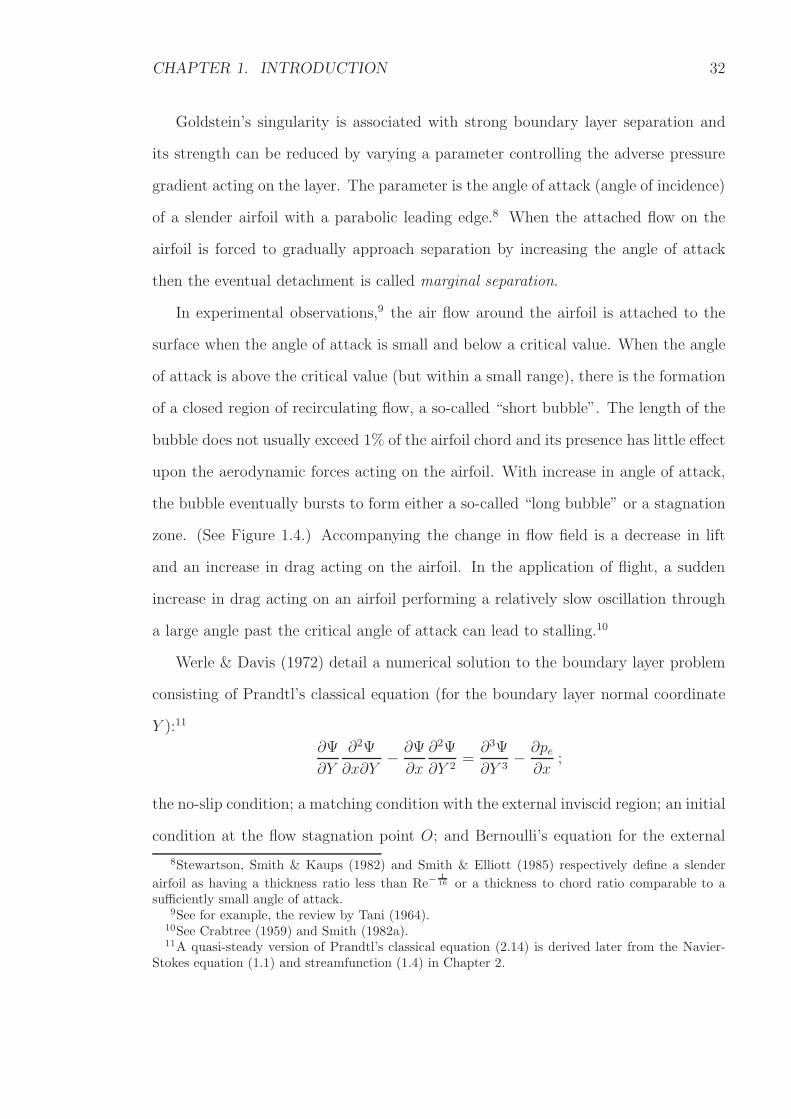
CHAPTER 1. INTRODUCTION 33
1
O
O
O
M
O’
y’
x’
α
Figure 1.4: The flow around an airfoil at angle of attack α with a short bubble, a longbubble, and an extended separation zone (from top to bottom). There is a stagnationpoint at O.
flow:
dpedx
= −Ue
dUe
dx.
The solutions are in terms of the skin friction and an asymmetry parameter k of the
parabolic nose. The parameter k is related to the angle of attack and similar to k
related to the position of separation mentioned in Section 1.3. The results from Werle
and Davies give support to the experimental observations.
The skin friction
τ =∂2Ψ
∂Y 2
∣
∣
∣
∣
Y=0
is parabolic in shape with a positive minimum. The minimum value of the skin
friction first vanishes for k0 = 1.1556 at a critical angle of attack αc and a point of
separation occurs at x = x0. When k < k0, the skin friction remains positive for all
x and has a minimum just beyond a point M where the pressure gradient is adverse.
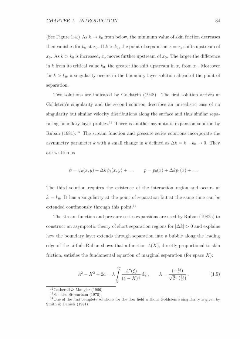
CHAPTER 1. INTRODUCTION 34
(See Figure 1.4.) As k → k0 from below, the minimum value of skin friction decreases
then vanishes for k0 at x0. If k > k0, the point of separation x = xs shifts upstream of
x0. As k > k0 is increased, xs moves further upstream of x0. The larger the difference
in k from its critical value k0, the greater the shift upstream in xs from x0. Moreover
for k > k0, a singularity occurs in the boundary layer solution ahead of the point of
separation.
Two solutions are indicated by Goldstein (1948). The first solution arrives at
Goldstein’s singularity and the second solution describes an unrealistic case of no
singularity but similar velocity distributions along the surface and thus similar sepa-
rating boundary layer profiles.12 There is another asymptotic expansion solution by
Ruban (1981).13 The stream function and pressure series solutions incorporate the
asymmetry parameter k with a small change in k defined as ∆k = k− k0 → 0. They
are written as
ψ = ψ0(x, y) + ∆kψ1(x, y) + . . . p = p0(x) + ∆kp1(x) + . . .
The third solution requires the existence of the interaction region and occurs at
k = k0. It has a singularity at the point of separation but at the same time can be
extended continuously through this point.14
The stream function and pressure series expansions are used by Ruban (1982a) to
construct an asymptotic theory of short separation regions for |∆k| > 0 and explains
how the boundary layer extends through separation into a bubble along the leading
edge of the airfoil. Ruban shows that a function A(X), directly proportional to skin
friction, satisfies the fundamental equation of marginal separation (for space X):
A2 −X2 + 2a = λ
∞∫
X
A′′(ξ)
(ξ −X)12
dξ , λ =(−1
4!)√
2 · (14!). (1.5)
12Catherall & Mangler (1966)13See also Stewartson (1970).14One of the first complete solutions for the flow field without Goldstein’s singularity is given by
Smith & Daniels (1981).
CHAPTER 1. INTRODUCTION 35
The integral on the right hand side stems from the pressure-displacement relationship
and the viscous-inviscid interaction between the viscous sublayer and the external
inviscid region. The parameter a, like k, is a constant directly proportional to the
departure of the angle of attack from its critical marginal value: |α− αc|.
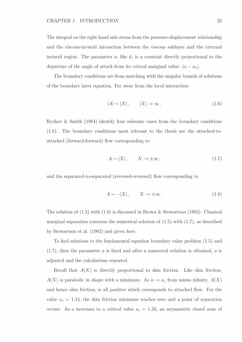
The boundary conditions are from matching with the singular branch of solutions
of the boundary layer equation. Far away from the local interaction:
|A| ∼ |X| , |X| → ∞ . (1.6)
Ryzhov & Smith (1984) identify four subsonic cases from the boundary conditions
(1.6). The boundary conditions most relevant to the thesis are the attached-to-
attached (forward-forward) flow corresponding to
A ∼ |X| , X → ±∞ ; (1.7)
and the separated-to-separated (reversed-reversed) flow corresponding to
A ∼ −|X| , X → ±∞ . (1.8)
The solution of (1.5) with (1.8) is discussed in Brown & Stewartson (1983). Classical
marginal separation concerns the numerical solution of (1.5) with (1.7), as described
by Stewartson et al. (1982) and given here.
To find solutions to the fundamental equation boundary value problem (1.5) and
(1.7), then the parameter a is fixed and after a numerical solution is obtained, a is
adjusted and the calculations repeated.
Recall that A(X) is directly proportional to skin friction. Like skin friction,
A(X) is parabolic in shape with a minimum. As a → as from minus infinity, A(X)
and hence skin friction, is all positive which corresponds to attached flow. For the
value as = 1.14, the skin friction minimum reaches zero and a point of separation
occurs. As a increases to a critical value ac = 1.33, an asymmetric closed zone of
CHAPTER 1. INTRODUCTION 36
recirculating flow grows in length and thickness, which coincides with negative skin
friction. For a > ac, there is only a complex solution.15 The assumption is that
the complex solution corresponds to short-bubble bursting and the formation of an
extended separation zone.
Stewartson et al. (1982) developed marginal separation theory independently; con-
firmed Ruban’s results but showed that the flow may assume various configurations
since there is non-uniqueness of solution. Quasi-steady hysteresis is shown to occur
when the roles of parameter a and A(X = 0) are interchanged.16 There is a lower
branch of solutions as ac → as which corresponds to either unseparated flow or a
local zone of separation. Brown & Stewartson (1983) refine the numerical solution
further to find for 0.60 < a < 0.68, there is a loop on the lower branch and there
are in fact four solutions. One solution is unseparated flow and the remaining three
solutions correspond to local zones of separation with the primary difference between
them being the length of the zone. The jump from one regime of flow to another is
known from experiments as the process that accompanies short-bubble bursting. As
a→ +0, where a = 0 is found to be a singular point on the lower branch, the point
of separation approaches x = 0 and the reattachment point of the bubble recedes
downstream to infinity.
1.5 Steady Flow on a Downstream-Moving Sur-
face
The theory of unsteady separation is reviewed by Sychev, Ruban, Sychev & Korolev
(1998c) and that of unsteady flows along moving walls by Sears & Telionis (1975).17
The appearance of Goldstein’s singularity on the surface and thus vanishing skin
15Chernyshenko (1985)16See also work by Kuryanov, Stolyarov & Steinberg (1979).17Care must be taken over terminology when switching between discussions on steady flows and
steady flows over downstream-moving surfaces. For example, Stewartson (1960) on the theory ofunsteady laminar boundary layers uses the term “separation” to denote vanishing wall shear and“breakdown” to denote separation.
CHAPTER 1. INTRODUCTION 37
friction, or wall shear stress, is adopted as the most general definition of separation
in the case of steady flow past fixed walls. However, “vanishing wall shear and
accompanying flow reversal near the wall, do not, in general denote separation in any
meaningful sense in unsteady flows.”18
An example of unsteady flow is the Blasius (1908) problem of flow past a circular
cylinder set into motion instantaneously from rest. At the first instant, the flow is
potential and is described by the solution for unseparated steady flow past a cylinder
with zero circulation. At the body surface, the no-slip condition is imposed. There
arises the process of vorticity diffusion and convection which leads to the formation of
a boundary layer.19 At a certain instant, the point of zero skin friction starts moving
upstream along the body surface from the rear stagnation point. The solution of the
unsteady boundary layer equations is regular although a point of zero skin friction
is located. At the point of vanishing wall shear, there is a region of reversed flow
direction within the boundary layer.
In contrast to steady flow problems, the appearance of reverse flow does not
lead to the violation of Prandtl’s hierarchical concept. Unsteady effects make it
possible for flow direction to reverse without the termination of the boundary layer
and the beginning of a wake, which produces global effects such as drag or buffeting.
Therefore, the appearance of a point of zero skin friction in an unsteady boundary
layer is not to be identified with the occurrence of flow separation. The circumstance
was first noted by Rott (1956), Sears (1956) and Moore (1958) when accounting
the flows produced when two-dimensional stagnation point flow is combined with
unsteady movement of the wall parallel to itself.
Prandtl’s separation criterion to encompass both unsteady flow and flow moving
past walls was generalised by Moore (1958). The criterion for unsteady separation
is best illustrated by an analogy between steady boundary layer separation from the
surface of a moving body and the separation of an unsteady boundary layer. Moore
18Rott (1956)19Lighthill (1963)
CHAPTER 1. INTRODUCTION 38
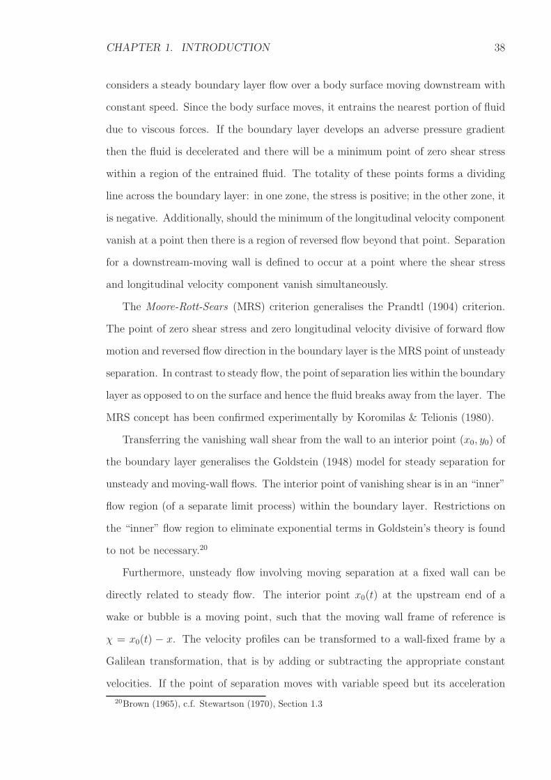
considers a steady boundary layer flow over a body surface moving downstream with
constant speed. Since the body surface moves, it entrains the nearest portion of fluid
due to viscous forces. If the boundary layer develops an adverse pressure gradient
then the fluid is decelerated and there will be a minimum point of zero shear stress
within a region of the entrained fluid. The totality of these points forms a dividing
line across the boundary layer: in one zone, the stress is positive; in the other zone, it
is negative. Additionally, should the minimum of the longitudinal velocity component
vanish at a point then there is a region of reversed flow beyond that point. Separation
for a downstream-moving wall is defined to occur at a point where the shear stress
and longitudinal velocity component vanish simultaneously.
The Moore-Rott-Sears (MRS) criterion generalises the Prandtl (1904) criterion.
The point of zero shear stress and zero longitudinal velocity divisive of forward flow
motion and reversed flow direction in the boundary layer is the MRS point of unsteady
separation. In contrast to steady flow, the point of separation lies within the boundary
layer as opposed to on the surface and hence the fluid breaks away from the layer. The
MRS concept has been confirmed experimentally by Koromilas & Telionis (1980).
Transferring the vanishing wall shear from the wall to an interior point (x0, y0) of
the boundary layer generalises the Goldstein (1948) model for steady separation for
unsteady and moving-wall flows. The interior point of vanishing shear is in an “inner”
flow region (of a separate limit process) within the boundary layer. Restrictions on
the “inner” flow region to eliminate exponential terms in Goldstein’s theory is found
to not be necessary.20
Furthermore, unsteady flow involving moving separation at a fixed wall can be
directly related to steady flow. The interior point x0(t) at the upstream end of a
wake or bubble is a moving point, such that the moving wall frame of reference is
χ = x0(t) − x. The velocity profiles can be transformed to a wall-fixed frame by a
Galilean transformation, that is by adding or subtracting the appropriate constant
velocities. If the point of separation moves with variable speed but its acceleration
20Brown (1965), c.f. Stewartson (1970), Section 1.3
CHAPTER 1. INTRODUCTION 39
is not large then this should not lead to qualitative changes in the flow structure in
comparison with that of a point of separation moving with constant speed.
Like self-induced and marginal separation, solutions of the unsteady boundary
layer equations are known to develop generic separation singularities in regions where
the pressure gradient is prescribed and adverse. The first interactive stage, governed
by the classical boundary layer equations, is where the solutions terminate in a singu-
larity. As the boundary layer starts to separate from the surface, the external pressure
distribution is altered though large-scale viscous-inviscid interaction just prior to the
formation of the singularity. This is referred to as the second interactive stage by
Cassel (2000). A numerical solution for the second interactive stage in unsteady
boundary layer separation has been obtained by Cassel, Smith & Walker (1996). As
an eruption develops, the boundary layer thickens and leads to the third interactive
stage of vortex-sheet formation. The solutions of the Navier-Stokes equations for
interaction in unsteady separation at large but finite Reynolds number, described by
Cassel (2000), support a sequence of events for flow induced by a “thick-core” vortex.
Unsteady boundary layer separation is discussed by Sears & Telionis (1971).
Boundary layer solution from a downstream-moving surface and subsequent singular-
ity analysis is given by Elliott, Smith & Cowley (1983). Furthermore, boundary layer
separation from a parabolic cylinder at an angle of incidence having a downstream-
moving surface is analysed by Telionis & Werle (1973). There is evidence of break-
down of the boundary layer equations well downstream of vanishing wall shear.
1.6 UnsteadyMarginal Separation & Dynamic Stall
Marginal separation theory can be extended to quasi-steady and unsteady fluid mo-
tion. Smith & Elliott (1985) consider the subcritical case where the angle of attack
is static, like in classical marginal separation theory, but flow is allowed to develop
on a very large time scale T compared to the boundary layer time scale t. The gov-
erning equation is the (normalised) unsteady fundamental equation for skin friction
CHAPTER 1. INTRODUCTION 40
parameter A(X, T ) and angle of attack parameter 2a = −1:
A2 −X2 + 2a =
X∫
−∞
∂A
∂T(ξ, T )
dξ
(X − ξ) 14
. (1.9)
The viscous-inviscid interaction integral on the right hand side of (1.5) is replaced
by the unsteady effects integral on the right hand side of (1.9). The marginal sepa-
ration and attached-to-attached flow motion case has the boundary conditions (1.7).
Solutions can be obtained from various initial conditions. A steady state solution:
A = (X2 + 1)12
appears to be approached as time becomes large, if the initial condition is sufficiently
smooth and close to the boundary conditions treated as a function of X :
A ∼ |X| , ∀X . (1.10)
In short, steady state streamlined flow can be preserved in some cases. Other initial
conditions not sufficiently close to the boundary conditions function (1.10) lead to a
singularity after a finite time.
Furthermore, Smith (1982a) introduces the concept of dynamic stall where there
is a relatively slow oscillation of the airfoil through a large angle of attack. The
change in angle of attack can cause the onset of the third interactive stage. Vortices
form at the leading edge of the airfoil which then travel along the airfoil towards
the trailing edge. When the vortices are eventually shed from the airfoil, the lift is
reduced and stall occurs.
The flow motion far away from the region of separation is taken to vary slowly with
time compared to the local interaction. The unsteady interaction region is of a triple-
deck structure with length scale x−xs of order Re−15 whilst the time scale is initially
long and of order Re−120 . The unsteady flow response is initially a small deviation
CHAPTER 1. INTRODUCTION 41
from the steady separation profile but is governed by the fully unsteady equation
of marginal separation, which is an unsteady, nonlinear, partial integro-differential
equation for skin friction parameter A(X, T ):
A2 −X2 + 2a =
∞∫
X
∂2A
∂ξ2(ξ, T )
dξ
(ξ −X)12
−X∫
−∞
∂A
∂T(ξ, T )
dξ
(X − ξ) 12
. (1.11)
Its derivation is adapted from Stewartson (1970) and is determined by the solvabil-
ity condition for the stream function, like the derivation of the steady fundamental
equation of marginal separation (1.5).
Smith (1982a), Ruban (1982b), Ryzhov & Smith (1984) and Elliott & Smith
(1987) study the Cauchy problem of (1.11) and the effect of instabilities. The main
result is that the perturbations of the steady solution are not damped with time.
The boundary layer displacement is progressively shifted upstream and increasing in
thickness. There is local behaviour of reversed flow, which is faster than the initial
response, on a shorter time scale of order Re−17 . Eventually, the displacement becomes
enormously accentuated and asymmetric. Accompanying the massive displacement
and reversed flow is wave-like behaviour, multiple vortices and their shedding from the
surface of the airfoil. Smith suggests a finite-time nonlinear breakdown is encountered
as T → Ts, when displacement becomes unbounded at a finite point of separation.
Furthermore, the dynamic stall process and nonlinear breakdown can occur in
subcritical conditions, when the angle of attack is less than the critical angle for the
steady fundamental equation (1.5). This is because any reversed flow encountered is
unstable to short-wavelength disturbances.21
The next stage in dynamic stall due to unsteady marginal separation is studied
by Elliott & Smith (1987). There is a new flow regime governed by a shortened
length scale of order Re−27 and time scale of order Re−
17 where the dimensions of the
recirculating vortex becomes comparable to the original boundary layer thickness.
The evolution of the vortex is a third interactive stage vortex-sheet problem.
21See Ruban (1982b) and Ryzhov & Smith (1984).
CHAPTER 1. INTRODUCTION 42
Recent Works
Work on marginal separation and steady flow over a moving surface has been extended
(post-1990) to three-dimensional flows, flows over obstacles, local suction flows and/or
all of the mentioned in order to control the flow, by Braun & Kluwick (2002), Braun
& Kluwick (2004), Braun & Kluwick (2005) and Hackmuller & Kluwick (1990a),
Hackmuller & Kluwick (1990b), and is reviewed by Braun (2006).
Detailed reviews on laminar separation flows including: compressible flows, flows
with suction and injection of fluid, flows with severe pressure gradients, boundary
layer interactions with shock waves, and wake studies are given by Brown & Stew-
artson (1969); boundary layer separation at supersonic speeds, supersonic ramp and
base flows, incompressible trailing edge flows, and turbulent flows are given by Mes-
siter (1979); high Reynolds number flows in channels and pipes by Smith (1982b);
breakdown of boundary layers on moving surfaces in unsteady flow by Elliott et al.
(1983); and boundary layer interaction theory on the trailing edge by Messiter (1983).
Work by Duck (1990) (and also Samad (2004)) extends the unsteady problem
to include three-dimensional effects; McCroskey (1982) studies unsteady oscillating
airfoils and their effects; Degani, Li & Walker (1996) (and also Stavrou (2004)) is
concerned with an abruptly-started airfoil and goes on to suggest localised control
measures such as suction to inhibit separation.
More recent work by Scheichl, Braun & Kluwick (2008) presents numerical com-
putation of the solutions leading to the finite-time breakdown, displacement thickness
and wall shear stress characteristics of the bubble bursting process.
Elliott & Smith (1987) on dynamic stall due to unsteady marginal separation
ends with a vortex-sheet problem spanning the boundary layer. Numerical solutions
of the Navier-Stokes equations for unsteady separation induced by a vortex are given
by Obabko & Cassel (2002b). The vortices eventually merge before being lifted away
from the surface. Obabko & Cassel (2002a) extends the problem to detachment of the
dynamic-stall vortex above a moving surface where it is found that increasing the wall
CHAPTER 1. INTRODUCTION 43
speed close to a critical value can supress unsteady separation and the detachment
of the vortex.
Another branch of research is the instability analysis of unsteady boundary layer
separation. Further work on the instability of Navier-Stokes solutions of unsteady
boundary layer separation has been done by Cassel et al. (1996); and on instability
caused by the vortex ejection has been done by Obabko & Cassel (2005) and Cassel
& Obabko (2010).
Objectives of the Thesis
The aim of the thesis is mentioned in Section 1.1 and is expanded upon here.
The thesis aims to bridge the work on marginal separation with that on steady
flow over a downstream-moving surface, unsteady marginal separation and dynamic
stall. In particular, the focus is on the quasi-steady flow structure about a point of
zero skin friction which develops over a very large time scale when there are very slow
perturbations to the otherwise steady stream functions. The slow perturbations are
from a slow change in angle of attack causing a downstream movement of the surface
only observable on the large time scale. (See Figure 1.1.) The angle of attack is over
a small range and it gradually approaches the critical angle where stream function
solutions become complex and nonlinear breakdown occurs. Furthermore, the time
scale is sufficiently large such that the induced pressure gradient by the displaced
boundary layer is of relatively small order of magnitude compared to the unsteady
or viscous forces acting on the boundary layer. The induced pressure gradient is
somewhat removed by the slow perturbations on the large time scale much like how
the strength of Goldstein’s singularity (and adverse pressure gradient) is reduced by
marginal separation theory.
The unsteady equation of marginal separation and solvability condition to be
solved is like (1.9) but the angle of attack parameter a is a function of the large
time scale. If the large time scale approaches a smaller asymptotic scale where the
induced pressure gradient is no longer negligible then the dynamic stall equation
CHAPTER 1. INTRODUCTION 44
(1.11) takes effect. If the induced pressure gradient is significant and the angle of
attack is static (and subcritical) then the flow is governed by the classical marginal
separation equation (1.5).
Chapter 2
Boundary Layer Analysis
To begin the boundary layer analysis, the external inviscid flow (region 1 in Figure 1.3)
must be considered first.
2.1 The External Inviscid Flow Region
A rectangular coordinate system O′x′y′ (which is not to be confused with a system
Oxy) is introduced, where the origin O′ coincides with the apex of the leading edge
of the airfoil and the axis O′x′ lies along the tangent to the mean line of the profile.
(See Figure 1.4.) In the external inviscid flow region, x′ and y′ are of order unity.
The airfoil is thin and of relative thickness ǫ such that the classical thin airfoil
theory applies. The thin airfoil theory states that the angle of attack is related to
lift for inviscid incompressible flows and that the pressure gradient on the surface is
also of order ǫ.1 The nose of the airfoil is assumed parabolic in shape such that the
surface can be described by the equations:
y′ = ǫF±(x′) , 0 ≤ x′ ≤ 1 ;
F±(x′) = ±
√2x′ + . . . x′ → 0 ,
where the positive and negative signs correspond to the top and underside of the
1Batchelor (2000b)
45
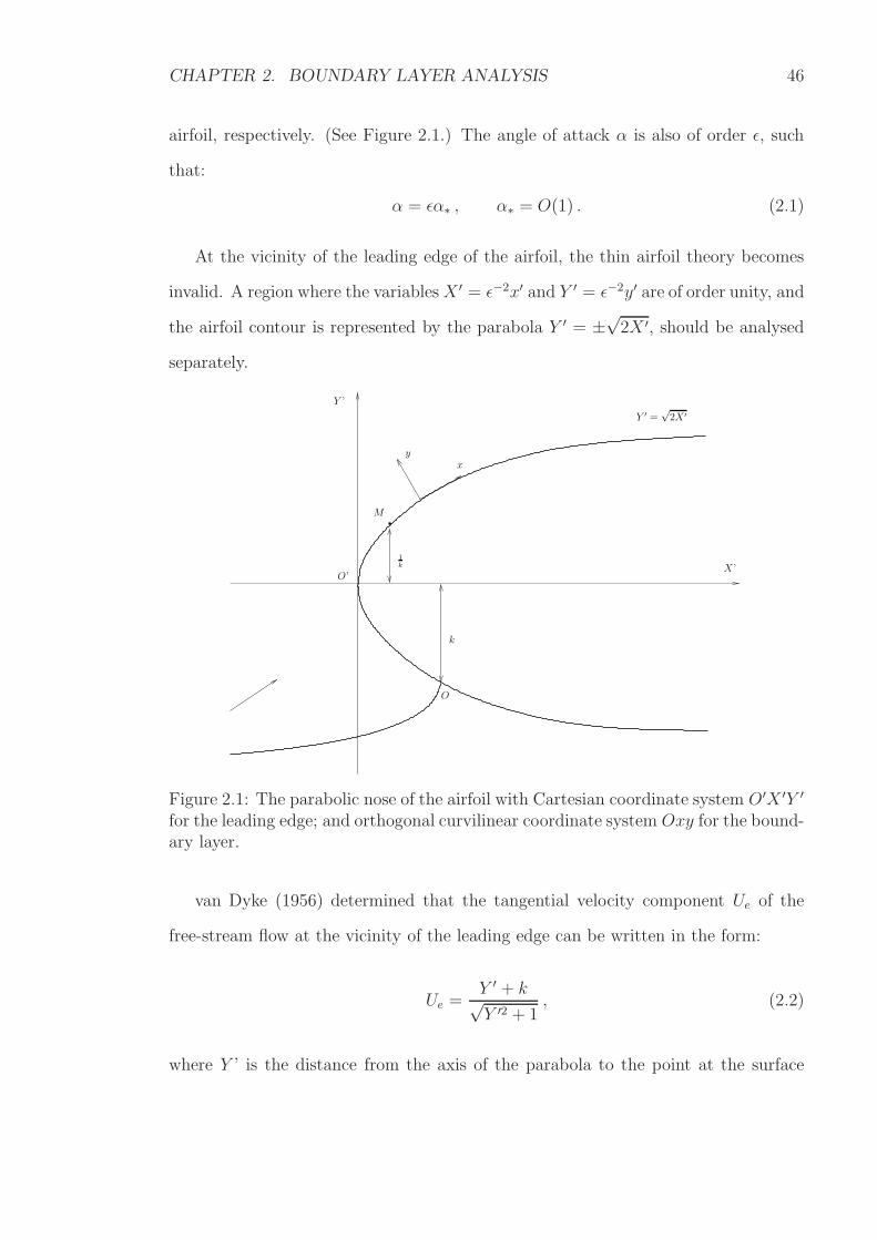
CHAPTER 2. BOUNDARY LAYER ANALYSIS 46
airfoil, respectively. (See Figure 2.1.) The angle of attack α is also of order ǫ, such
that:
α = ǫα∗ , α∗ = O(1) . (2.1)
At the vicinity of the leading edge of the airfoil, the thin airfoil theory becomes
invalid. A region where the variablesX ′ = ǫ−2x′ and Y ′ = ǫ−2y′ are of order unity, and
the airfoil contour is represented by the parabola Y ′ = ±√2X ′, should be analysed
separately.
1k
x
Y ′ =√2X ′
X ’
k
O
O’
M
y
Y ’
Figure 2.1: The parabolic nose of the airfoil with Cartesian coordinate system O′X ′Y ′
for the leading edge; and orthogonal curvilinear coordinate system Oxy for the bound-ary layer.
van Dyke (1956) determined that the tangential velocity component Ue of the
free-stream flow at the vicinity of the leading edge can be written in the form:
Ue =Y ′ + k√Y ′2 + 1
, (2.2)
where Y ’ is the distance from the axis of the parabola to the point at the surface
CHAPTER 2. BOUNDARY LAYER ANALYSIS 47
where the speed is to be calculated. The parameter k, where
k =√2
α∗ +1
π
1∫
0
G(x′)√
x′(1− x′)dx′
, (2.3)
G = −12
(
dF+
dx′+
dF−
dx′
)
,
is a representation of the flow asymmetry near the leading edge in terms of the angle
of attack α∗ (2.1). The stagnation point is given by Y ′ = −k and for example, when
k = 0, the stagnation point is at the parabola vertex.
2.2 The Boundary Layer
The orthogonal curvilinear coordinate system Oxy (which is not to be confused with
the external inviscid flow region Cartesian coordinate system O′x′y′), where x lies
along the upper surface of the airfoil from stagnation point O and y is normal to
the surface, is preferable when examining the boundary layer at the vicinity of the
leading edge of the airfoil. (See Figure 2.1.)
The non-dimensionalised Navier-Stokes equations in two-dimensional orthogonal
curvilinear coordinates x and y, are:
∂u
∂t+u
h
∂u
∂x+ v
∂u
∂y+κvu
h=
1
Re
∂
∂y
(
1
h
[
∂(hu)
∂y− ∂v
∂x
])
− 1
h
∂p
∂x, (2.4)
∂v
∂t+u
h
∂v
∂x+ v
∂v
∂y+κu2
h= − 1
Re
1
h
∂
∂x
(
1
h
[
∂(hu)
∂y− ∂v
∂x
])
− ∂p
∂y, (2.5)
∂u
∂x+∂(hv)
∂y= 0 , (2.6)
where
h = 1 + κ(x)y .
The dimensionless curvature κ(x) of the body surface is defined as positive for a
CHAPTER 2. BOUNDARY LAYER ANALYSIS 48
convex wall when the centre of curvature is located on the side y < 0.2 Similarly,
the stream function equations in two-dimensional orthogonal curvilinear coordinates
x and y, are:
u =∂ψ
∂y, (1 + κ(x)y)v = −∂ψ
∂x. (2.7)
To leading order, the equations in orthogonal curvilinear coordinates (2.4), (2.5),
(2.6) and (2.7) return to the equations in Cartesian coordinates (1.1), (1.2), (1.3)
and (1.4).
The boundary layer extends along the surface of the airfoil and hence the longi-
tudinal coordinate x and velocity component u are of order unity. From the balance
of inertial and viscous terms in the first, x-momentum equation (1.1):
u∂u
∂x+ v
∂u
∂y∼ 1
Re
(
∂2u
∂x2+∂2u
∂y2
)
.
Hence, to leading order, the thickness of the boundary layer is of order Re12 such that
the normal coordinate to the surface is
Y = Re12y = O(1) ; (2.8)
the normal velocity component is
V = Re12 v = O(1) ; (2.9)
and the stream function is:
Ψ = Re12ψ = O(1) . (2.10)
As the air flow is of high speed and low viscosity, the limit as Re → ∞ may be
taken. A viscous term: ∂2u∂x2 cannot be balanced with the O(1) terms. However, the
term: ∂2u∂Y 2 is present and the x-momentum equation is not singular.
The conditions to be satisfied are:
2Rosenhead (1963)
CHAPTER 2. BOUNDARY LAYER ANALYSIS 49
1. the no-slip conditions on the surface:
Ψ =∂Ψ
∂Y= 0 , Y = 0 ; (2.11)
2. the condition of matching of the boundary layer with the external inviscid
region. The stream function Ψ must not grow exponentially as Y →∞.
Only a local region of the point of zero skin friction x = xs is considered and so
the variable:
s = x− xs = O(1) (2.12)
is introduced. It is noted that (−s) is positive for the region upstream of the point
of zero skin friction.
The Time Scale
The airfoil is subject to a very slow perturbation only observable on a very large time
scale T compared to the external region time scale t, such that
T = σ−1t = O(1) , σ →∞ . (2.13)
The perturbation is a slow change in angle of attack of the airfoil causing a downstream-
movement of the surface. (See Figure 1.1.) The change in angle of attack is charac-
terised by k (2.3), which is now a function of time T . (See Figure 2.1.) At the critical
value k = k0 is the first appearance of a point of zero skin friction x = xs. The small
variable:
∆k = k(T )− k0 → 0
is introduced to represent the small change in angle of attack. On the external region
time scale t is steady flow over a fixed surface such that the no-slip conditions (2.11)
apply. Meanwhile, on the boundary layer time scale T , there are slow and small
O(∆k) perturbations to the steady flow caused by the slow and small change in angle
CHAPTER 2. BOUNDARY LAYER ANALYSIS 50
of attack.
Taking the limits as Re → ∞, σ → ∞, s = O(1) and ∆k → 0 in the boundary
layer (regions 2 and 3 in Figure 1.3), the x-momentum equation to leading order
becomes the boundary layer equation:
1
σ
∂2Ψ
∂T∂Y+∂Ψ
∂Y
∂2Ψ
∂x∂Y− ∂Ψ
∂x
∂2Ψ
∂Y 2=∂3Ψ
∂Y 3− ∂pe∂x
, (2.14)
where pe is the pressure at the outer edge of the boundary layer.
When the parameter k differs slightly from its critical value k0, the asymptotic
series expansion of the tangential velocity about k = k0 in the external inviscid region
is:
Ue(x, k) = Ue(x, k0) + ∆k∂Ue
∂k
∣
∣
∣
∣
k=k0
+ . . .
By Bernoulli’s equation, there is a similar series expansion for pressure, that is
pe = p0(x, Y ) + ∆kp1(x, Y, T ) +∆k
σp2(x, Y, T ) + . . .
where p0(x, Y ) is the pressure for flow over a static airfoil. The series expansion of
the pressure gradient is
∂pe∂x
= λ0 + λ1s+ . . . (2.15)
for s (2.12). The corresponding series expansion of the stream function Ψ(x, Y, T ) is
defined as:
Ψ = Re12ψ = Ψ0(x, Y ) + ∆kΨ1(x, Y, T ) +
∆k
σΨ2(x, Y, T ) + . . . (2.16)
The steady flow is represented by the term: Ψ0(x, Y ). The flow perturbation is
represented by the term: ∆kΨ1(x, Y, T ). The unsteady perturbation effects on the
flow are exhibited by the forcing term: ∆kσΨ2(x, Y, T ).
To allow for quasi-steady flow, the constants arising from the stream function
perturbation solutions Ψ1(x, Y, T ) and Ψ2(x, Y, T ) become functions of time T . Their
CHAPTER 2. BOUNDARY LAYER ANALYSIS 51
effects are only perceived on this large time scale and not on the external inviscid
region time scale t.
2.3 Ψ0(x, Y ) Solution
From the boundary layer equation (2.14), stream function (2.16) and pressure gradi-
ent (2.15) series expansions, and the no-slip conditions (2.11):
∂3Ψ0
∂Y 3
∣
∣
∣
∣
Y=0
=dpedx
= λ0 .
At the point of zero skin friction, by definition:
τ =∂2Ψ0
∂Y 2
∣
∣
∣
∣
Y=0
= 0 . (2.17)
Hence, the leading term of the asymptotic representation of the stream function at
the vicinity of the point of zero skin friction is
Ψ0 =1
6λ0Y
3 + . . . = O(Y 3) . (2.18)
The length scales of the viscous flow region are determined by the stream function
(2.18), and the balance of the orders of magnitude of viscous and inertia terms in the
boundary layer equation (2.14):
∂Ψ0
∂Y
∂2Ψ0
∂x∂Y∼ ∂3Ψ0
∂Y 3.
Hence, the longitudinal scale decreases according to Y = O[(−s) 14 ] as s→ −0 and a
similarity variable of the viscous flow region can be defined as:
η =Y
(−s) 14
= O(1) . (2.19)
CHAPTER 2. BOUNDARY LAYER ANALYSIS 52
The stream function (2.18) becomes
Ψ0 = (−s)− 341
6λ0η
3 + . . .
The asymptotic expansion for the steady stream function Ψ0(x, Y ) is sought in the
form
Ψ0 = (−s) 341
6λ0η
3 + (−s)αf01(η) + (−s)2α− 34 f02(η) + . . . (2.20)
where the second term is an eigenfunction with an unknown eigenvalue α and the
third term is a forcing term arising from the square of the second term. The forcing
term appears in the expansion due to the nonlinearity of the boundary layer equation
(2.14). Substituting the expansion into the boundary layer equation and taking the
limit as s→ −0, then differential equations for f01(η) and f02(η) are obtained.
2.3.1 f01(η) Solution
The f01(η) equation is
f ′′′01 −
1
8λ0η
3f ′′01 +
1
2λ0
(
α+1
4
)
η2f ′01 − λ0αηf01 = 0 (2.21)
with the no-slip conditions:
f01(η) = f ′01(η) = 0 , η = 0 .
Three linearly independent solutions can be constructed for (2.21) in such a way that
their Taylor series expansions about the point η = 0 start with either 1, η or η2.
However, only the solution starting with η2 satisfies the no-slip conditions. Hence, a
non-trivial solution of (2.21) for any eigenvalue α is
f01(η) =1
2a0η
2 . (2.22)
CHAPTER 2. BOUNDARY LAYER ANALYSIS 53
The arbitrary constant a0 depends on the external inviscid flow, Ue.
2.3.2 f02(η) Solution
The f02(η) equation is
f ′′′02 −
1
8λ0η
3f ′′02 + λ0
(
α− 1
4
)
η2f ′02 − λ0
(
2α− 3
4
)
ηf02 =1
4(1− 2α) a20η
2 (2.23)
with the no-slip conditions:
f02(η) = f ′02(η) = 0 , η = 0
and the matching condition with the external inviscid region. The solution should
not grow exponentially as η → ∞. The general solution is the linear concatenation
of the contemporary solution for the homogeneous form of (2.23) and the particular
solution. The contemporary solution for the homogeneous equation is
f c02(η) =
1
2b0η
2
from the same reasons as in Section 2.3.1, where b0 is an arbitrary constant. A
description of the Frobenius method to find the particular solution of an equation
similar to (2.23) is described in Sections 2.6.1 and 2.6.2. The particular solution is
f p02(η) =
1
2
a20λ0
(η − hα(η))
where
hα(η) = η − η2η∫
0
η−21
[
1F1
(
1− 2α;5
4;λ032η41
)
− 1
]
dη1 (2.24)
and 1F1
(
1− 2α; 54; λ0
32η4)
is a confluent hypergeometric function. The general solution
is therefore
f02(η) =1
2b0η
2 +1
2
a20λ0
(η − hα(η)) (2.25)
CHAPTER 2. BOUNDARY LAYER ANALYSIS 54
with hα (2.24).3
2.3.3 Confluent Hypergeometric Functions
The confluent hypergeometric function 1F1(a; b; z) is defined4 throughout the entire
complex plane z, as
1F1(a; b; z) =∞∑
n=0
(a)n(b)n
zn
n!(2.26)
where the Pochhammer symbol (a)n is defined as:
(a)n = (a)(a+ 1) . . . (a+ n− 1) , (a)0 = 1 . (2.27)
When |z| is large and a and b are fixed, then
1F1(a; b; z) = e±iπaz−a Γ(b)
Γ(b− a)
R−1∑
n=0
(a)n(1 + a− b)nn!
(−z)−n +O(
|z|−R)
+ ezza−b Γ(b)
Γ(a)
S−1∑
n=0
(b− a)n(1− a)nn!
z−n +O(
|z|−S)
(2.28)
where the upper sign is taken if −12π < arg z < 3
2π, the lower sign is −3
2π < arg z ≤
−12π. The Gamma function Γ is defined as
Γ(b) = (b− 1)! =
∞∫
0
tb−1e−t dt , ℜ(t) > 0 . (2.29)
The behaviour of the the general solution (2.25) can be determined as the point
of zero skin friction is approached or when the outer edge of the boundary layer is
approached, that is as η → ∞. To match at the outer edge of the boundary layer,
the general solution, and consequently the confluent hypergeometric function from
(2.24), cannot grow exponentially as η →∞. When
1− 2α = −m, m = 0, 1, 2, . . . (2.30)
3Sychev et al. (1998b)4See, for example, Abramovich & Stegun (1972).
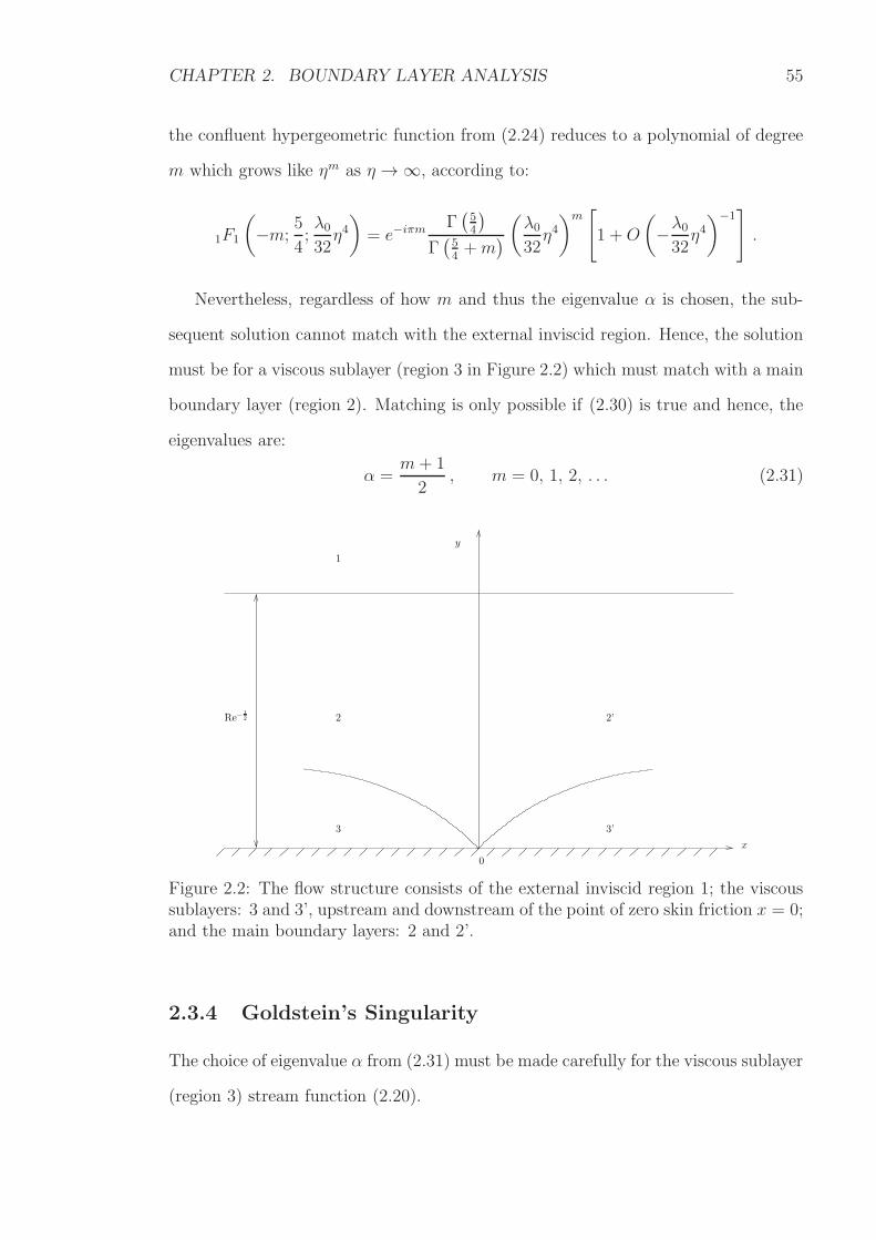
CHAPTER 2. BOUNDARY LAYER ANALYSIS 55
the confluent hypergeometric function from (2.24) reduces to a polynomial of degree
m which grows like ηm as η →∞, according to:
1F1
(
−m;5
4;λ032η4)
= e−iπmΓ(
54
)
Γ(
54+m
)
(
λ032η4)m[
1 +O
(
−λ032η4)−1
]
.
Nevertheless, regardless of how m and thus the eigenvalue α is chosen, the sub-
sequent solution cannot match with the external inviscid region. Hence, the solution
must be for a viscous sublayer (region 3 in Figure 2.2) which must match with a main
boundary layer (region 2). Matching is only possible if (2.30) is true and hence, the
eigenvalues are:
α =m+ 1
2, m = 0, 1, 2, . . . (2.31)
2
3
1
2’
3’
0
y
x
Re−12
Figure 2.2: The flow structure consists of the external inviscid region 1; the viscoussublayers: 3 and 3’, upstream and downstream of the point of zero skin friction x = 0;and the main boundary layers: 2 and 2’.
2.3.4 Goldstein’s Singularity
The choice of eigenvalue α from (2.31) must be made carefully for the viscous sublayer
(region 3) stream function (2.20).
CHAPTER 2. BOUNDARY LAYER ANALYSIS 56
For α = 12(m = 0), (2.20) becomes
Ψ0 = (−s) 341
6λ0η
3 + (−s) 12 f01(η) + (−s)− 1
4 f02(η) + . . .
where each successive term is of a smaller order of magnitude then the preceding
term. This does not make sense by definition of the asymptotic expansion.
For α = 1 (m = 1), (2.20) becomes
Ψ0 = (−s) 341
6λ0η
3 + (−s)f01(η) + (−s) 54f02(η) + . . . (2.32)
with f01(η) and f02(η) given by (2.22) and (2.25) respectively. In particular,
f01(η) =1
2a0η
2 , f02(η) =1
2b0η
2 − 1
2 · 5!a20η
5 + . . .
The subsequent hierarchical analysis (as illustrated in Figure 2.3), for the viscous
sublayer (region 3 in Figure 2.2) to the main boundary layer (region 2) and the regions
3’ and 2’ downstream of the point of zero skin friction, leads to a contradiction and
Goldstein’s singularity.5
To determine a solution for the main boundary layer (region 2) where Y = O(1), a
change of variables from η (2.19) to (−s)− 14Y is made in the viscous sublayer (region
3) stream function Ψ0 (2.32). Collecting terms of the same order of magnitude as
s→ −0 then gives
Ψ0 =1
6λ0Y
3 + (−s) 121
2a0Y
2 + . . .
Hence, the series expansion solution for the main boundary layer (region 2) should
be sought in the form
Ψ0 = Ψ00(Y ) + (−s) 12Ψ01(Y ) + . . . (2.33)
The solution should match with the outer edge of the viscous sublayer (region 3), of
5See Hartree (1939) and Goldstein (1948).
CHAPTER 2. BOUNDARY LAYER ANALYSIS 57
which the stream function components (2.32) when η = (−s)− 14Y , are:
Ψ00 =1
6λ0Y
3 − 1
2 · 5!a20Y
5 + . . . , Ψ01 =1
2a0Y
2 + . . . , Y → 0 . (2.34)
Substituting (2.33) into the boundary layer equation (2.14) and taking into account
the conditions of matching (2.34), then
Ψ01 =a0λ0
dΨ00
dY
and hence,
Ψ0 = Ψ00(Y ) + (−s) 12a0λ0
dΨ00
dY+ . . .
The transverse velocity component
V = Re12 v = (−s)− 1
21
2
a0λ0
dΨ00
dY+ . . . (2.35)
exhibits singular behaviour as s → −0, that is as the point of zero skin friction is
approached from upstream. The skin friction:
τ =∂2Ψ
∂Y 2
∣
∣
∣
∣
Y=0
= (−s) 12a0 + . . .
The transverse velocity component V = O[(−s)− 12 ] exhibits Goldstein’s singularity.
For a non-zero coefficient a0, the solution cannot be extended beyond the point of
zero skin friction. The argument for this is by contradiction.
Suppose that the solution can be extended continuously through the point of zero
skin friction. By continuity of the boundary layer (region 2), the leading term of the
series expansion for the boundary layer (region 2’) downstream of the point of zero
skin friction coincides with (2.33):
Ψ0 = Ψ00(Y ) + . . . s→ +0 . (2.36)
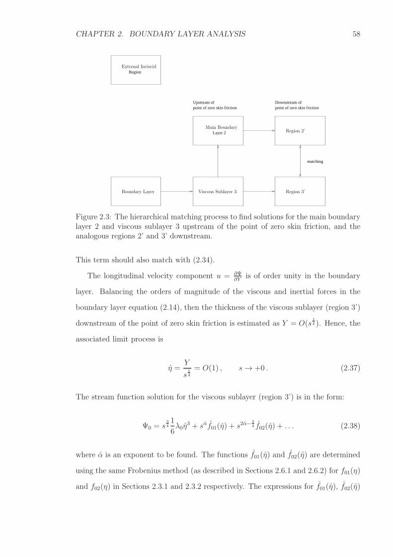
CHAPTER 2. BOUNDARY LAYER ANALYSIS 58
Downstream of
matching
Upstream of
Layer 2
point of zero skin friction point of zero skin friction
Region
Boundary Layer
Main BoundaryRegion 2’
Region 3’Viscous Sublayer 3
External Inviscid
Figure 2.3: The hierarchical matching process to find solutions for the main boundarylayer 2 and viscous sublayer 3 upstream of the point of zero skin friction, and theanalogous regions 2’ and 3’ downstream.
This term should also match with (2.34).
The longitudinal velocity component u = ∂Ψ∂Y
is of order unity in the boundary
layer. Balancing the orders of magnitude of the viscous and inertial forces in the
boundary layer equation (2.14), then the thickness of the viscous sublayer (region 3’)
downstream of the point of zero skin friction is estimated as Y = O(s14 ). Hence, the
associated limit process is
η =Y
s14
= O(1) , s→ +0 . (2.37)
The stream function solution for the viscous sublayer (region 3’) is in the form:
Ψ0 = s341
6λ0η
3 + sαf01(η) + s2α−34 f02(η) + . . . (2.38)
where α is an exponent to be found. The functions f01(η) and f02(η) are determined
using the same Frobenius method (as described in Sections 2.6.1 and 2.6.2) for f01(η)
and f02(η) in Sections 2.3.1 and 2.3.2 respectively. The expressions for f01(η), f02(η)
CHAPTER 2. BOUNDARY LAYER ANALYSIS 59
are
f01 =1
2a0η
2 ,
f02 =1
2b0η
2 +1
2
a0λ0
(η2 − hα) ,
where
hα = η − η2η∫
0
η−21
[
1F1
(
1− 2α;5
4;−λ0
32η41
)
− 1
]
dη1 ;
a0, b0 are arbitrary constants; and 1F1
(
1− 2α; 54;−λ0
32η4)
is a confluent hypergeomet-
ric function. The behaviour of the confluent hypergeometric function is described in
Section 2.3.3.
As the outer edge of region 3’ is approached from below and η → ∞, the hyper-
geometric function behaves like
1F1
(
1− 2α;5
4;−λ0
32η4)
= e−iπmΓ(
54
)
Γ(
14+ 2α
)
(
−λ032η4)−1+2α
[
1 +O
(
λ032η4)−1
]
and hence, the function:
f02 =1
2
a20λ0
Γ(
54
)
Γ(
14+ 2α
)
(
λ032
)−1+2αη8α−3
8α− 5+ . . .
Therefore, the stream function (2.38) at the outer edge of region 3’, with the change
of variable from η (2.37) to s−14Y , is
Ψ0 =1
6λ0Y
3 +1
2
a20λ0
Γ(
54
)
Γ(
14+ 2α
)
(
λ032
)−1+2αY 8α−3
8α− 5+ . . . (2.39)
As the inner edge of region 2’ is approached from above, the series expansion
(2.36) by condition of matching (2.34) becomes:
Ψ0 =1
6λ0Y
3 − 1
2 · 5!a20Y
5 + . . . , Y → 0 . (2.40)
According to the principle of matched asymptotic expansions, the expression
CHAPTER 2. BOUNDARY LAYER ANALYSIS 60
(2.34) for main boundary layer (region 2) upstream of the point of zero skin fric-
tion should match with the downstream (region 2’) expression (2.40). Therefore,
α = 1
and the region 3’ expression (2.39) becomes:
Ψ0 =1
6λ0Y
3 +1
2 · 5! a20Y
5 + . . . (2.41)
Crucially, matching the region 3’ expression (2.41) with the region 2’ expression (2.40)
gives
a20 = −a20 . (2.42)
The constant a0 is found from the process of solving the boundary layer equations
with an initial upstream cross section x = 0 up to the point of zero skin friction. The
constant (2.42) determines a0 for the solution downstream, which is imaginary. This
means that a real solution ahead of the point of zero skin friction is impossible. A
real solution is only obtained when a0 = 0 and the first eigenfunction is absent. For
a0 6= 0, the transverse velocity component (2.35) grows without bound as s → ±0
and the boundary layer hypothesis ceases to be valid.
A triple-deck interaction region in the neighbourhood of the point of zero skin
friction is created where the displacement of streamlines from the surface no longer
has a negligible effect on the external flow and leads to a redistribution of pressure
along the boundary layer. (See Figure 2.4.) The middle layer (region II) is analogous
to the main boundary layer (region 2). If Goldstein’s singularity is true then solutions
for the interaction region cease to exist since the flow profile in region 2’ must match
with that of the interaction region II. A change in longitudinal velocity component
u is small in high Reynolds number flow, that is
∆u→ 0 , Re→∞
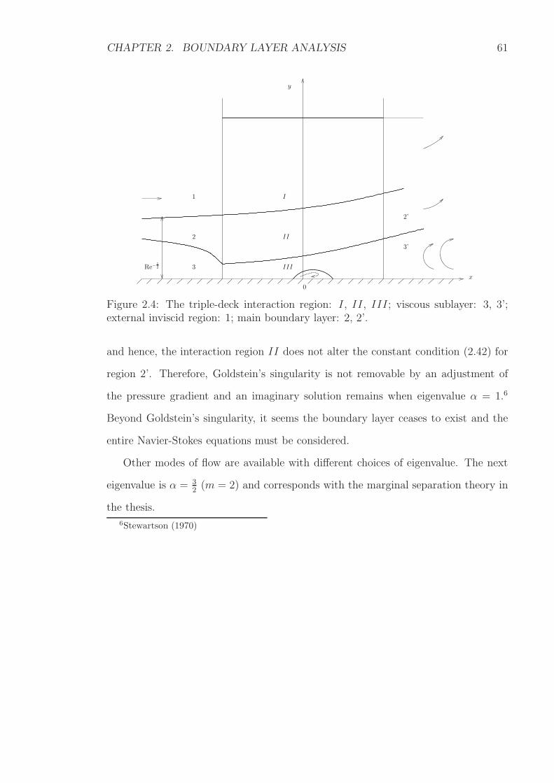
CHAPTER 2. BOUNDARY LAYER ANALYSIS 61
1
2
2’
3’
0
3
II
I
III
y
x
Re−12
Figure 2.4: The triple-deck interaction region: I, II, III; viscous sublayer: 3, 3’;external inviscid region: 1; main boundary layer: 2, 2’.
and hence, the interaction region II does not alter the constant condition (2.42) for
region 2’. Therefore, Goldstein’s singularity is not removable by an adjustment of
the pressure gradient and an imaginary solution remains when eigenvalue α = 1.6
Beyond Goldstein’s singularity, it seems the boundary layer ceases to exist and the
entire Navier-Stokes equations must be considered.
Other modes of flow are available with different choices of eigenvalue. The next
eigenvalue is α = 32(m = 2) and corresponds with the marginal separation theory in
the thesis.
6Stewartson (1970)
CHAPTER 2. BOUNDARY LAYER ANALYSIS 62
2.3.5 The Steady Airfoil General Solution
The eigenvalue is α = 32and the steady stream function Ψ0(x, Y ) in the viscous
sublayer (region 3) is
Ψ0 = (−s) 341
6λ0η
3 + (−s) 321
2a0η
2
+ (−s) 74
[
−16λ1η
3 +2
7!λ0λ1η
7
]
+ (−s) 94
[
1
2b0η
2 − 1
5!a20η
5 +1
8!λ0a
20η
9
]
+ . . . (2.43)
where the second term (−s) 3212a0η
2 is the first eigenfunction; λ0, λ1 are the coefficients
for the leading terms in expansion of the pressure gradient (2.15); and a0, b0 are
constants.7 The solution (2.43) can be extended continuously through the point of
zero skin friction unlike the solution for eigenvalue α = 1: (2.32), and the proof is by
the following regional construction. (See Figure 2.3.)
By the same method as in the previous Section 2.3.4, the steady stream function
(2.43) is written in the variables η = (−s)− 14Y and hence, the stream function in the
main boundary layer (region 2) is of the form:
Ψ0 = Ψ00(Y ) + (−s)Ψ01(Y ) + . . . s→ −0 , (2.44)
which should match with (2.43) as Y → 0. Substituting (2.44) into the boundary
layer equation (2.14) and gathering the O(1) terms then
−Ψ′00Ψ
′01 +Ψ01Ψ
′′00 = −λ0 +Ψ′′′
00 , (2.45)
with the notation:
Ψ′00 =
dΨ00
dY, Ψ′′′
00 =d3Ψ00
dY 3.
The region 2 Ψ01 equation (2.45), divided by (Ψ′00)
2 and integrated with respect to
7For an airfoil with a parabolic leading edge then a0 = 0.0085 by Sychev et al. (1998b).
CHAPTER 2. BOUNDARY LAYER ANALYSIS 63
Y , becomes the solution:
Ψ01 = Ψ′00
c0 +
Y∫
0
λ0 −Ψ′′′00
(Ψ′00)
2dY
(2.46)
where, from the condition of matching between (2.43) and (2.44), the constant of
integration is
c0 =a0λ0
; (2.47)
and
Ψ00 =1
6λ0Y
3 +2
7!λ0λ1Y
7 +1
8!λ0a
20Y
9 + . . . Y → 0 . (2.48)
Next, the solutions ahead of the point of zero skin friction are constructed. By
the previous method, the solution for region 2’ (as shown in Figure 2.2) is sought in
the form:
Ψ0 = Ψ00(Y ) + sΨ01(Y ) + . . . s→ +0 . (2.49)
The region 2’ Ψ01 equation is obtained from substitution of (2.49) into the boundary
layer equation, in a similar fashion for (2.45). Like (2.46), the equation is satisfied if
Ψ01 = Ψ′00
c0 +
Y∫
0
λ0 −Ψ′′′00
(Ψ′00)
2dY
(2.50)
where
c0 =a0λ0.
Matching with the main boundary layer (region 2) implies Ψ00 (2.48) still applies.
Finally, the solution for region 3’ is sought in the form:
Ψ0 = s341
6λ0η
3 + s34 f01(η) + s
74 F01(η) + s
94 f02(η) + . . . s→ +0 . (2.51)
Substituting (2.51) into the boundary layer equation and taking into account the
CHAPTER 2. BOUNDARY LAYER ANALYSIS 64
no-slip conditions gives
f01 =1
2a0η
2 ,
F01 =1
6λ1η
3 +2
7!λ0λ1η
7 ,
f02 =1
2b0η
2 +1
5!a20η
5 +1
8!λ0a
20η
9 .
The solutions for regions 2’ (2.49) and 3’ (2.51) can match because the constant
relation
a20 = a20 (2.52)
is found to admit real solutions for these regions downstream of the point of zero skin
friction.
One region 3’ expression, given by a0 = a0, is
Ψ0 = Ψ00(Y ) + Ψ′00
a0λ0|s|+ s
Y∫
0
Ψ′′′00 − λ0(Ψ′
00)2
dY
+O(s2) .
The angle of inclination θ of the streamlines in the boundary layer is given by
Re12θ = −
∂Ψ0
∂x∂Ψ0
∂Y
= −a0λ0
sign(s) +
Y∫
0
Ψ′′′00 − λ0(Ψ′
00)2
dY +O(s) (2.53)
and undergoes a discontinuity when passing through the point of zero skin friction
at s = 0. The skin friction behaves as
τ =∂2Ψ0
∂Y 2
∣
∣
∣
∣
Y=0
= a0|s|+O(
s2)
, s→ 0 .
Hence, the a0 = a0 expression is singular.
When a0 = −a0, there is the region 3’ solution:
Ψ0 = Ψ00(Y ) + Ψ′00
−a0λ0s+ s
Y∫
0
Ψ′′′00 − λ0(Ψ′
00)2
dY
+O(s2) (2.54)
CHAPTER 2. BOUNDARY LAYER ANALYSIS 65
which can be continued smoothly through the point of zero skin friction. The skin
friction behaves as
τ = −a0s+O(s2) , s→ 0
and becomes negative past the point of zero skin friction, when s becomes positive.
This is evidence of a region of reverse flow downstream.8 Again, matching with the
viscous sublayer (region 3) implies Ψ00 (2.48) still applies.
2.4 Ψ1(x, Y, T ) Solution
When ∆k 6= 0 and the parameter k differs slightly from its critical value k0, there
are perturbations Ψ1 to the steady flow Ψ0. The Ψ1 analysis is given in Sychev et al.
(1998b).
Substituting the stream function series expansion (2.16) into the boundary layer
equation (2.14) and collecting terms of order ∆k then the Ψ1 equation:
∂Ψ0
∂Y
∂2Ψ1
∂x∂Y+∂2Ψ0
∂x∂Y
∂Ψ1
∂Y− ∂Ψ0
∂x
∂2Ψ1
∂Y 2− ∂2Ψ0
∂Y 2
∂Ψ1
∂x= −dp1
dx+∂3Ψ1
∂Y 3(2.55)
is obtained. The solution is subject to the no-slip conditions:
Ψ1 =∂Ψ1
∂Y= 0 , Y = 0
and the condition of no exponential growth as Y →∞.
The solutions for (2.55) in the viscous sublayer (region 3) and main boundary
layer (region 2) are constructed, in that order, using the same methods as shown in
Section 2.3. The region 3 Ψ0 terms are from (2.43).
For the viscous sublayer (region 3), the perturbation Ψ1 is sought in the form:
Ψ1 = (−s)βf11(η) + (−s)β+ 14f12(η) + . . . s→ −0 (2.56)
8Ruban (1981)
CHAPTER 2. BOUNDARY LAYER ANALYSIS 66
where β is the eigenvalue to be found. Substituting (2.56) into (2.55) and solving
using the Frobenius method then
f11 =1
2a1η
2 ,
f12 =1
2b1η
2 +a0a1λ0
(η − hβ)
where
hβ = η − η2η∫
0
η−21
[
1F1
(
−(
β +1
2
)
;5
4;λ032η41
)
− 1
]
dη1 .
The confluent hypergeometric function 1F1
(
−(
β + 12
)
; 54; λ0
32η4)
and hence hβ do not
grow exponentially as η →∞ when
β = m− 1
2, m = 0, 1, 2, . . .
The function hβ = η with the smallest eigenvalue β = 12. Therefore, the Ψ1 solution
for the region 3 is
Ψ1 = (−s)− 121
2a1η
2 + (−s) 141
2b1η
2 + . . . (2.57)
The arbitrary constants a1 and b1 are determined by conditions of matching with
the outer edge of the boundary layer as Y →∞ and matching with the initial cross
section as x→ −∞.
Taking into account the viscous sublayer (region 3) solution (2.57), then by the
method of matched asymptotic expansions, the main boundary layer (region 2) stream
function is
Ψ1 = (−s)−1 a1λ0a1
dΨ00
dY+O
[
(−s)− 14
]
, s→ −0 . (2.58)
The condition of matching (2.48) implies
Ψ00 =1
6λ0Y
3 +2
7!λ0λ1Y
7 +1
8!λ0a
20Y
9 + . . . Y → 0 .
CHAPTER 2. BOUNDARY LAYER ANALYSIS 67
The solution (2.58) grows without bound as the point of zero skin friction is ap-
proached. Hence, a neighbourhood about the point must be analysed separately as
the interaction region in Chapter 3.
2.5 Ψ0(x, Y, T ) & Ψ1(x, Y, T ) Solutions by Region
The stream function (2.16) solutions
Ψ = Re12ψ = Ψ0(x, Y ) + ∆kΨ1(x, Y, T ) +
∆k
σΨ2(x, Y, T ) + . . .
by regions in Figure 2.5, are summarised.
1. The leading viscous sublayer (region 3) stream function components are Ψ0
(2.43):
Ψ0 = (−s) 341
6λ0η
3 + (−s) 321
2a0η
2
+ (−s) 74
[
−16λ1η
3 +2
7!λ0λ1η
7
]
+ (−s) 94
[
1
2b0η
2 − 1
5!a20η
5 +1
8!λ0a
20η
9
]
+ . . .
and Ψ1 (2.57):
Ψ1 = (−s)− 121
2a1η
2 + (−s) 141
2b1η
2 + . . .
for similarity variable (2.19):
η =Y
(−s) 14
= O(1) .
2. The leading main boundary layer (region 2) stream function components are
Ψ0 (2.44) and Ψ1 (2.58). The Ψ0 component is
Ψ0 = Ψ00(Y ) + (−s)Ψ01(Y ) + . . . s→ −0
CHAPTER 2. BOUNDARY LAYER ANALYSIS 68
where from matching with the viscous sublayer (region 3), (2.48):
Ψ00 =1
6λ0Y
3 +2
7!λ0λ1Y
7 +1
8!λ0a
20Y
9 + . . . Y → 0 (2.59)
and (2.46):
Ψ01 = Ψ′00
a0λ0
+
Y∫
0
λ0 −Ψ′′′00
(Ψ′00)
2dY
.
The Ψ1 component is
Ψ1 = (−s)−1 a1λ0a1
dΨ00
dY+O
[
(−s)− 14
]
, s→ −0 .
3. The leading region 2’ stream function component is Ψ0 (2.49):
Ψ0 = Ψ00(Y ) + sΨ01(Y ) + . . . s→ +0 .
where (2.50):
Ψ01 = Ψ′00
−a0λ0
+
Y∫
0
λ0 −Ψ′′′00
(Ψ′00)
2dY
and matching with the main boundary layer (region 2) implies Ψ00(Y ) is (2.59).
4. The leading region 3’ stream function component is Ψ0 (2.51):
Ψ0 = s341
6λ0η
3 + s341
2a0η
2
+ s74
[
1
6λ1η
3 +2
7!λ0λ1η
7
]
+ s94
[
1
2b0η
2 +1
5!a20η
5 +1
8!λ0a
20η
9
]
+ . . . s→ +0
for similarity variable (2.37):
η =Y
s14
= O(1) .
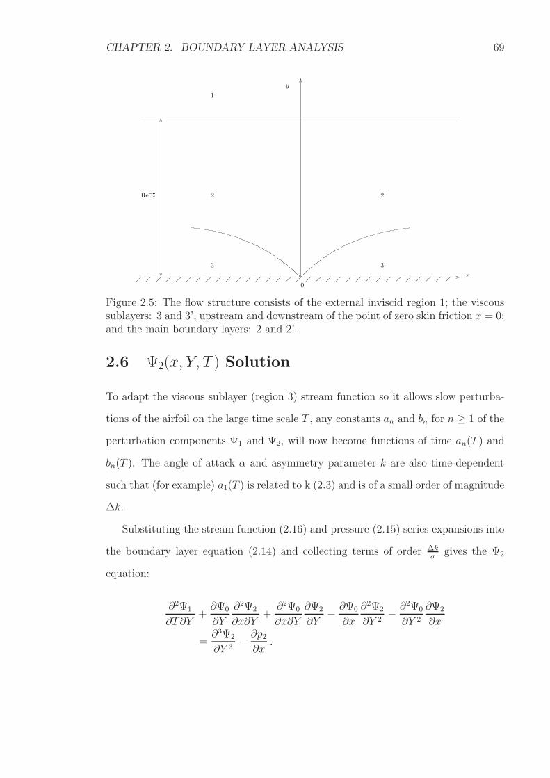
CHAPTER 2. BOUNDARY LAYER ANALYSIS 69
2
3
1
2’
3’
0
y
x
Re−12
Figure 2.5: The flow structure consists of the external inviscid region 1; the viscoussublayers: 3 and 3’, upstream and downstream of the point of zero skin friction x = 0;and the main boundary layers: 2 and 2’.
2.6 Ψ2(x, Y, T ) Solution
To adapt the viscous sublayer (region 3) stream function so it allows slow perturba-
tions of the airfoil on the large time scale T , any constants an and bn for n ≥ 1 of the
perturbation components Ψ1 and Ψ2, will now become functions of time an(T ) and
bn(T ). The angle of attack α and asymmetry parameter k are also time-dependent
such that (for example) a1(T ) is related to k (2.3) and is of a small order of magnitude
∆k.
Substituting the stream function (2.16) and pressure (2.15) series expansions into
the boundary layer equation (2.14) and collecting terms of order ∆kσ
gives the Ψ2
equation:
∂2Ψ1
∂T∂Y+∂Ψ0
∂Y
∂2Ψ2
∂x∂Y+∂2Ψ0
∂x∂Y
∂Ψ2
∂Y− ∂Ψ0
∂x
∂2Ψ2
∂Y 2− ∂2Ψ0
∂Y 2
∂Ψ2
∂x
=∂3Ψ2
∂Y 3− ∂p2∂x
.
CHAPTER 2. BOUNDARY LAYER ANALYSIS 70
Next, substituting for the region 3 terms Ψ0 (2.43) and Ψ1 (2.57) gives the Ψ2 equa-
tion:
∂3Ψ2
∂Y 3+
1
2λ0(−s)
12 η2
∂2Ψ2
∂x∂Y− a0(−s)
14η∂Ψ2
∂Y
+1
2a0(−s)
12 η2
∂2Ψ2
∂Y 2− λ0(−s)
14 η∂Ψ2
∂x
= (−s)− 34 a1η −
∂p2∂x
, (2.60)
with the notation:
a1(T ) ≡da
dT.
The no-slip conditions:
Ψ2 =∂Ψ2
∂Y= 0 , Y = 0 (2.61)
and the condition of no exponential growth at the outer edge of the viscous sublayer
apply. It is necessary to impose a condition at the initial cross section x = 0 but the
specific form of this condition is unimportant for the analysis at this stage. Addition-
ally, the pressure perturbation p2 will not balance in the analysis, like the pressure
term p1 in the Ψ1 analysis.
The asymptotic expansion for Ψ2 is sought in a similar form to the series expan-
sions (2.20) and (2.56) for Ψ0 and Ψ1, such that
Ψ2 = (−s)γf21(η, T ) + (−s)γ+ 34 f22(η, T ) + . . . (2.62)
where η is the similarity variable (2.19). The exponents are chosen in such a way to
include the unsteady term a1(T ) in the solution; and γ 6= 0 is the eigenvalue to be
found.
f21(x, Y, T ) Solution
Substitution of (2.62) and viscous sublayer terms Ψ0 (2.43) and Ψ1 (2.57) into the Ψ2
equation (2.60), then gathering terms of the same order of magnitude as (−s) → 0,
CHAPTER 2. BOUNDARY LAYER ANALYSIS 71
gives the f21(η, T ) equation:
f ′′′21 −
1
8λ0η
3f ′′21 +
1
2λ0η
2
(
γ +1
4
)
f ′21 − λ0ηγf21 = 0 .
From (2.61), the appropriate no-slip conditions are
f21(0, T ) = f ′21(0, T ) = 0 , ∀T .
The general solution is:
f21 =1
2a2(T )η
2 , ∀ γ (2.63)
where a2(T ) remains arbitrary until an initial profile condition is imposed.
f22(x, Y, T ) Solution
To determine the eigenvalue γ, it is necessary to consider the f22(η, T ) equation:
(−s)γ[
f ′′′22 −
1
8λ0η
3f ′′22 +
1
2(γ + 1)λ0η
2f ′22 −
(
γ +3
4
)
λ0ηf22
]
= (−s)− 34 a1η + (−s)γ
[
3
4a0η
2f ′′21 − a0(γ + 1)ηf ′
21 − a0γf21]
.
Setting the eigenvalue
γ = −34
(2.64)
ensures that the equation captures the unsteady effects of a1(T ) and hence:
f ′′′22 −
1
8λ0η
3f ′′22 +
1
8λ0η
2f ′22 = a1η +
7
8a0a2η
2 . (2.65)
The conditions are
f22(0, T ) = f ′22(0, T ) = 0 , ∀T (2.66)
and that f22(η, T ) does not grow exponentially as η →∞.
For a complimentary solution of (2.65), note that the equation is third order and
CHAPTER 2. BOUNDARY LAYER ANALYSIS 72
so three linearly independent Taylor series solutions can be constructed about the
point η = 0 which begin with either 1, η or η2. However, only the solution like η2 is
non-trivial after applying (2.66). Therefore, the complimentary solution is:
f c22 =
1
2b2(T )η
2 , (2.67)
where b2(T ) remains arbitrary until an initial condition is imposed.
The particular solution of (2.65) is the linear combination of the particular solu-
tions of the equations:
f ′′′22 −
1
8λ0η
3f ′′22 +
1
8λ0η
2f ′22 = a1η (2.68)
f ′′′22 −
1
8λ0η
3f ′′22 +
1
8λ0η
2f ′22 =
7
8a0a2η
2 . (2.69)
2.6.1 a1(T )η Particular Solution by Frobenius Method
The behaviour of the particular solution f p122 (η, T ) for (2.68) can be found from the
balance of the orders of magnitude of the viscous and unsteady forces in the Ψ2
equation (2.60), where
∂3Ψ2
∂Y 3∼ (−s)− 3
4 a1η = (−s)−1a1Y .
Only a small vicinity of the point of zero skin friction is considered, hence:
∆Ψ2
∆Y 3∼ (−s)−1a1Y
which implies
Ψ2 ∼ (−s)−1a1Y4 = a1η
4 .
CHAPTER 2. BOUNDARY LAYER ANALYSIS 73
In fact, if the f ′′′22(η, T ) term of (2.68) is balanced with the term on the right hand
side then the behaviour of the particular solution is also expected to be of the form:
f p122 ∼ a1η
4 .
If instead, the f ′22(η, T ) term is balanced with the term on the right hand side then
the particular solution has logarithmic behaviour and is expected to behave like:
f p122 ∼
8
λ0a1 ln η , η →∞ .
When η is of order unity, η = 0 is a regular point and hence the particular solution
can be obtained in the form of a Frobenius series:
f p122 =
∞∑
i=0
ci(T )ηi+α , (2.70)
where α is an unknown exponent (which is not to be confused with the eigenvalue
from Section 2.3). The functions of time ci(T ) are analogous to b2(T ) in (2.67) and
by definition, c0(T ) 6= 0. Substituting (2.70) into (2.68) and making an index shift
of i to i− 4 in the second and third term on the left hand side, gives the equation:
∞∑
i=0
ci(i+ α)(i+ α− 1)(i+ α− 2)ηi+α−3
− 1
8λ0
∞∑
i=4
ci−4(i+ α− 4)(i+ α− 6)ηi+α−3
= a1η .
For i = 0:
c0α(α− 1)(α− 2)ηα−3 = ηa1 .
To satisfy the definition c0(T ) 6= 0 then the exponent is
α = 4
CHAPTER 2. BOUNDARY LAYER ANALYSIS 74
and
c0 =1
4!a1 .
For i = 1:
c1(α + 1)α(α− 1)ηα−2 = ηa1
and with α = 4 then c1(T ) = 0. Analogously, c2(T ) = c3(T ) = 0. For i = 4m,
m = 1, 2, 3, . . . and noting the change of subscript for all ci(T ):
[
cm(i+ 4)(i+ 3)(i+ 2)− 1
8λ0i(i− 2)cm−1
]
ηi+1 = ηa1 .
Upon rearrangement, there is a recurrence relation for cm(T ):
cm =λ032
m(m− 12)
(m+ 1)(m+ 34)(m+ 2
4)cm−1 , c0 =
1
4!a1 .
Hence, for all m ≥ 1:
cm =
(
λ032
)m m(m− 12)
(m+ 1)(m+ 34)(m+ 2
4)
(m− 1)(m− 32)
m(m− 14)(m− 2
4). . .
1 · 12
2 · 74· 64
1
4!a1 ,
and after cancelation of terms, cm(T ) can be written:
cm =1
2 · 4!(1)m(74)m
(
λ032
)m1
m! · (m+ 1)(m+ 12)a1 ,
with the Pochhammer symbol (a)m defined as (2.27).
Therefore, (2.70) is:
f p122 =
1
2 · 4! a1η4
∞∑
m=0
(1)m(74)m
(λ0
32η4)m
m!
1
(m+ 1)(m+ 12)
or in terms of confluent hypergeometric functions:
f p122 =
1
3a1
η∫
0
η2
η2∫
0
η1 1F1
(
1;7
4;λ032η41
)
dη1 dη2 .
CHAPTER 2. BOUNDARY LAYER ANALYSIS 75
The confluent hypergeometric function 1F1
(
1; 74; λ0
32η41)
is defined as (2.26):
1F1
(
1;7
4;λ032η41
)
=∞∑
n=0
(1)n(74)n
(
λ0
32η41)n
n!.
Therefore, the particular solution is:
f p122 =
1
3a1
[
1
8η4 +
1
84
(
λ032
)
η8 + . . .
]
, η = O(1) (2.71)
with the expected O(a1η4) behaviour. Additionally, (2.71) satisfies the no-slip con-
ditions (2.66).
As η →∞, the confluent hypergeometric function behaves like
1F1
(
1;7
4;λ032η4)
= −Γ(74)
Γ(34)
(
32
λ0η−4
)
·[
R−1∑
m=0
(−1)m(
1
4
)
m
(
λ032η4)−m
+O
(
∣
∣
∣
λ032η4∣
∣
∣
−R)
]
, η →∞ (2.72)
and satisfies the condition of no exponential growth. Hence, the particular solution
(2.71) also satisfies the condition. The expected logarithmic behaviour is seen in
Section 2.7 with matching at the outer edge of the viscous sublayer with the inner
edge of the main boundary layer.
2.6.2 a2(T )η2 Particular Solution
A particular solution f p222 (η, T ) for (2.69) can be found from balancing the f ′
22(η, T )
term and the right hand side term. A particular solution is:
f p222 =
7
λ0a0a2η . (2.73)
Nevertheless, upon application of the no-slip conditions (2.66) then
a2(T ) = 0 (2.74)
CHAPTER 2. BOUNDARY LAYER ANALYSIS 76
since a0 6= 0 to avoid a non-trivial steady solution Ψ0.
If a2 6= 0 then another particular solution for (2.69) is found using the Frobenius
method analogous to that described for finding (2.71). Beginning with the Frobenius
series:
f p222 =
∞∑
j=0
dj(T )ηj+β , d0(T ) 6= 0
(where the exponent β is not to be confused with the eigenvalue from Section 2.4)
then
β = 5
so that
d0 =7
4 · 5!a0a2 .
For n = 1, 2, . . .
dn =7
16 · 4!(34)n
(74)n
(
λ032
)n1
n! · (n+ 1)(n+ 54)a0a2 , d0 =
7
4 · 5!a0a2 .
Hence, the solution is:
f p222 =
7
4!a0a2
η∫
0
η2∫
0
η31 1F1
(
3
4;7
4;λ032η41
)
dη1 dη2 .
The confluent hypergeometric function:
1F1
(
3
4;7
4;λ032η4)
= −Γ(74)
Γ(34)e
λ032
η4(
32
λ0η−4
)
·[
S−1∑
n=0
(
1
4
)
n
(
λ032η4)−n
+O
(
∣
∣
∣
λ032η4∣
∣
∣
−S)
]
, η →∞
grows exponentially without bound. To satisfy the condition of no exponential growth
and thus, to ensure matching with the external region as η →∞ then the confluent
hypergeometric function must be removed by making a2(T ) = 0.
CHAPTER 2. BOUNDARY LAYER ANALYSIS 77
2.7 The Viscous Sublayer
The general solution for the f22 equation (2.65), from combining the complimentary
(2.67) and non-trivial particular (2.71) solutions, is
f22 =1
2b2(T )η
2 +1
3a1
[
1
8η4 +
1
84
(
λ032
)
η8 + . . .
]
. (2.75)
The Ψ2 stream function (2.62); from (2.63), (2.64), (2.74) and (2.75); is also:
Ψ2 =1
2b2(T )η
2 +1
3a1
[
1
8η4 +
1
84
(
λ032
)
η8 + . . .
]
+ . . . (2.76)
Hence, the stream function (2.16) for the viscous sublayer is
Ψ =
(−s) 341
6λ0η
3 + (−s) 321
2a0η
2 + (−s) 74
[
−16λ1η
3 +2
7!λ0λ1η
7
]
+ (−s) 94
[
1
2b0η
2 − 1
5!a20η
5 +1
8!λ0a
20η
9
]
+ . . .
+∆k
(−s)− 121
2a1η
2 + (−s) 141
2b1η
2 + . . .
+∆k
σ
1
2b2(T )η
2 +1
3a1
[
1
8η4 +
1
84
(
λ032
)
η8 + . . .
]
+ . . . (2.77)
which is valid for η = O(1) by (2.19), with (−s) given by (2.12). When ∆k 6= 0
and as σ → ∞, there is a slow O(∆k) perturbation to the steady stream function
(2.43) as the angle of attack changes with a1(T ) ∼ ∆k. Perturbations of O(∆kσ) are
proportional to rate of change of angle of attack with respect to time as parameterised
by a1(T ). The larger the angle of attack and the faster its increase then the greater
the perturbations.
As the point of zero skin friction is approached and (−s)→ 0, there seems to be a
singularity caused by the O(∆kσ) perturbation. Further analysis of the flow structure
must incorporate the interaction region in Chapter 3.
CHAPTER 2. BOUNDARY LAYER ANALYSIS 78
Matching at the Outer Viscous Sublayer
As η →∞, the main boundary layer is approached from the viscous sublayer below.
Upon substitution of the confluent hypergeometric function (2.72) into the Ψ2 solution
(2.76), then
Ψ2 =1
2b2η
2 − 1
3a1
Γ(74)
Γ(34)
(
32
λ0
)
η∫
0
η2
η2∫
0
η−31 dη1 dη2
− 1
3a1
Γ(74)
Γ(34)
(
32
λ0
) R−1∑
m=1
(−1)m(
1
4
)
m
(
32
λ0
)m
·
η∫
0
η2
η2∫
0
η−4m−31 dη1 dη2
+ . . . (2.78)
The first integral:
1
3a1
Γ(74)
Γ(34)
(
32
λ0
)
η∫
0
η2
η2∫
0
η−31 dη1 dη2
=1
3!
Γ(74)
Γ(34)
(
32
λ0
)
a1 ln η ,
and the second integral:
1
3a1
Γ(74)
Γ(34)
(
32
λ0
) R−1∑
m=1
(−1)m(
1
4
)
m
(
32
λ0
)m
η∫
0
η2
η2∫
0
η−31 dη1 dη2
=1
3a1
Γ(74)
Γ(34)
(
32
λ0
) R−1∑
m=1
(−1)m(
1
4
)
m
(
32
λ0
)m [1
(−4m+ 2)(−4m)η−4m
]
.
Therefore, the most significant terms of (2.78) are from the first integral which have
the expected logarithmic behaviour. As η →∞:
Ψ2 =1
2b2η
2 +1
3a1
[
1
2
Γ(74)
Γ(34)
32
λ0ln η + . . .
]
+ . . . (2.79)
CHAPTER 2. BOUNDARY LAYER ANALYSIS 79
The stream function expansion for the viscous sublayer as η →∞, to match with the
main boundary layer, is:
Ψ =
(−s) 341
6λ0η
3 + (−s) 321
2a0η
2 + . . .
+ (−s) 94
[
1
2b0η
2 − 1
5!a20η
5 +1
8!λ0a
20η
9
]
+ . . .
+∆k
(−s)− 121
2a1η
2 + (−s) 141
2b1η
2 + . . .
+∆k
σ
1
2b2η
2 +1
3a1
[
1
2
Γ(74)
Γ(34)
32
λ0ln η + . . .
]
+ . . .
+ . . . (2.80)
2.8 The Main Boundary Layer
The main boundary layer (region 2) corresponds to the simple displacement of the
boundary layer by the viscous sublayer (region 3), whilst the sublayer exists to ensure
that the no-slip conditions are satisfied at the wall. It is of the same limit process as
the viscous sublayer as given by (2.8), (2.12) and (2.13). A change of variables η =
(−s)− 14Y is made in (2.79) then terms of the same order of magnitude as (−s) → 0
are gathered to obtain the Ψ2 stream function perturbation for the main boundary
layer:
Ψ2 =1
3!
Γ(74)
Γ(34)
32
λ0a1 lnY −
1
4!
Γ(74)
Γ(34)
32
λ0a1 ln(−s) + (−s)− 1
21
2b2Y
2 + . . .
CHAPTER 2. BOUNDARY LAYER ANALYSIS 80
From the principle of matched asymptotic expansions and (2.80), the main boundary
layer stream function as Y → 0 is like:
Ψ =1
6λ0Y
3
+
(−s)[
1
2a0Y
2 − 1
2 · 5!a20Y
5 + . . .
]
+ (−s) 74
[
1
2b0Y
2 + . . .
]
+ . . .
+∆k
(−s)−11
2a1Y
2 + (−s)− 141
2b1Y
2 + . . .
+∆k
σ
(−s)− 241
2b2Y
2 +1
3!
Γ(74)
Γ(34)
(
32
λ0
)
a1
[
lnY − 1
4ln(−s)
]
+ . . .
+ . . . (2.81)
Hence, the rate of change in angle of attack a1(T ) has a logarithmic perturbing effect
on the main boundary layer close to the point of zero skin friction.
Chapter 3
The Interaction Region
Further analysis of the flow structure must incorporate another region about the point
of zero skin friction with a new limit process. There is an interaction region (regions I,
II, III in Figure 2.4) where the boundary layer analysis fails. The displacement of the
streamlines from the boundary layer no longer have a negligible effect on the external
inviscid flow and eigenfunctions (2.43), (2.57), (2.76) in the series expansion (2.77)
for the viscous sublayer become the same order of magnitude. The same hierarchical
process in Chapter 2 is used to determine stream function solutions there. The stream
function solutions and triple-deck structure are consistent by the method of matched
asymptotic expansions if a solvability condition is satisfied.
Furthermore, there are small perturbations due to a slow change in angle of attack
of the airfoil on a large time scale T compared to the external region time scale t,
such that (2.13):
T = σ−1t = O(1) , σ →∞ .
The change in angle of attack is characterised by an asymmetry parameter k(T ) (2.3)
(See Figure 2.1.) At the critical value k = k0 is the first appearance of a point of zero
skin friction x = xs. The small variable:
∆k = k(T )− k0 → 0
81
CHAPTER 3. THE INTERACTION REGION 82
represents the small change in angle of attack.
The stream function of the form (2.16):
Ψ = Re12ψ = Ψ0(x, Y ) + ∆kΨ1(x, Y, T ) +
∆k
σΨ2(x, Y, T ) + . . .
for the viscous sublayer (2.77) is :
Ψ =
(−s) 341
6λ0η
3 + (−s) 321
2a0η
2 + (−s) 74
[
−16λ1η
3 +2
7!λ0λ1η
7
]
+ (−s) 94
[
1
2b0η
2 − 1
5!a20η
5 +1
8!λ0a
20η
9
]
+ . . .
+∆k
(−s)− 121
2a1η
2 + (−s) 141
2b1η
2 + . . .
+∆k
σ
1
2b2(T )η
2 +1
3a1
[
1
8η4 +
1
84
(
λ032
)
η8 + . . .
]
+ . . .
The first eigenfunctions of the first, steady series Ψ0 and the second, perturbation
series ∆kΨ1, which are the second term of Ψ0: (−s) 3212a0η
2 and the first term of
∆kΨ1: ∆k(−s)−1212a1η
2, become the same order of magnitude in a region where
(−s) = O(
|∆k| 12)
. (3.1)
The second eigenfunction term of the perturbation series ∆kΨ1: ∆k(−s)1412b1η
2 and
the first eigenfunction of the third, forcing series (∆kσ)Ψ2: (
∆kσ)12b2η
2 become the same
order of magnitude in a region where
(−s) = O(
σ−4)
. (3.2)
The boundary layer stream function collapses to an interaction region stream function
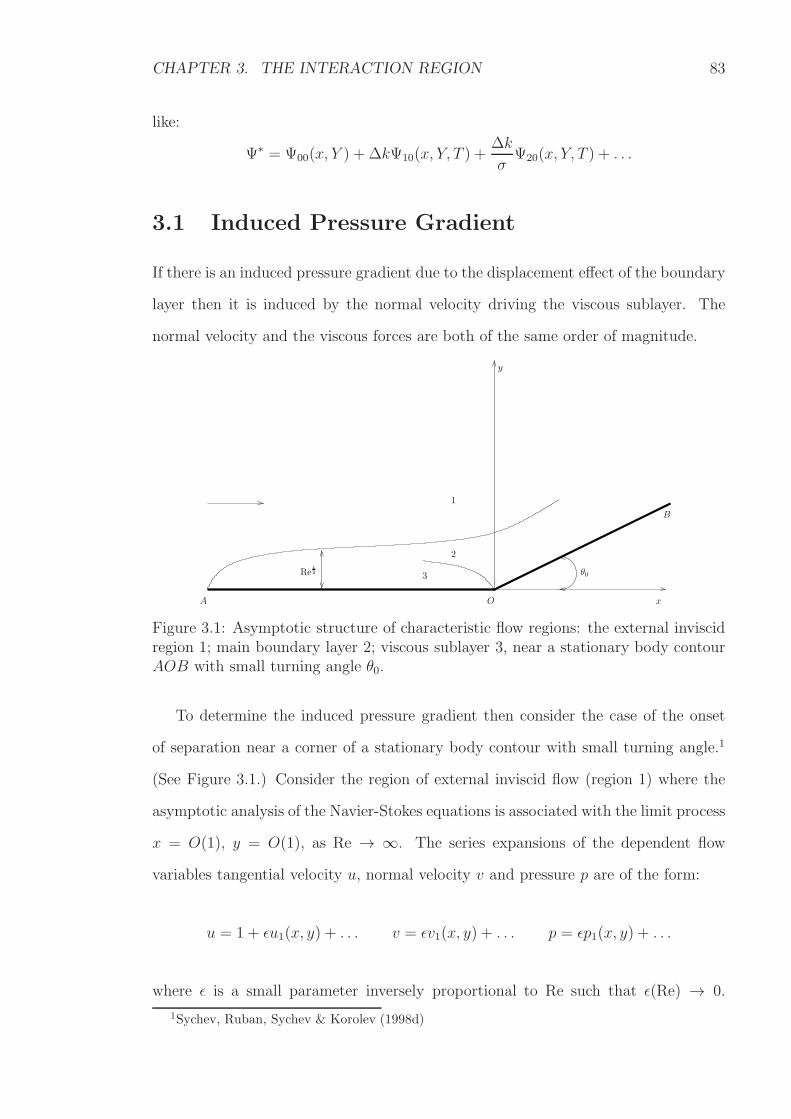
CHAPTER 3. THE INTERACTION REGION 83
like:
Ψ∗ = Ψ00(x, Y ) + ∆kΨ10(x, Y, T ) +∆k
σΨ20(x, Y, T ) + . . .
3.1 Induced Pressure Gradient
If there is an induced pressure gradient due to the displacement effect of the boundary
layer then it is induced by the normal velocity driving the viscous sublayer. The
normal velocity and the viscous forces are both of the same order of magnitude.
3
y
xOA
B
2
1
Re12 θ0
Figure 3.1: Asymptotic structure of characteristic flow regions: the external inviscidregion 1; main boundary layer 2; viscous sublayer 3, near a stationary body contourAOB with small turning angle θ0.
To determine the induced pressure gradient then consider the case of the onset
of separation near a corner of a stationary body contour with small turning angle.1
(See Figure 3.1.) Consider the region of external inviscid flow (region 1) where the
asymptotic analysis of the Navier-Stokes equations is associated with the limit process
x = O(1), y = O(1), as Re → ∞. The series expansions of the dependent flow
variables tangential velocity u, normal velocity v and pressure p are of the form:
u = 1 + ǫu1(x, y) + . . . v = ǫv1(x, y) + . . . p = ǫp1(x, y) + . . .
where ǫ is a small parameter inversely proportional to Re such that ǫ(Re) → 0.
1Sychev, Ruban, Sychev & Korolev (1998d)
CHAPTER 3. THE INTERACTION REGION 84
From the Navier-Stokes equations, the linearised Euler equations for u1, v1 and p1
are obtained. It follows that the complex velocity
w1(z) = u1 − iv1 , z = x+ iy
is an analytic function and the pressure perturbation satisfies the linearised Bernoulli
equation
p1 = −u1 .
The flow regime is such that separation is either absent or is localised within a small
neighbourhood of the corner. The boundary condition at the surface of the solid
body is the condition of no normal flow:
v1(x, 0) = 0 , −1 < x < 0 ;
v1(x, 0) = θ0 , 0 < x < l
where l is the dimensionless length of the plate OB and θ0 is the small turning angle
of the contour. (See Figure (3.1).) The condition uniquely determines the leading
series expansion term of the function w1 in the vicinity of the corner:
w1 =θ0πln z + d− iθ + o(1) , |z| → 0 .
The constant d can only be determined by solving the flow problem for the entire
external inviscid flow taking into account all the boundary conditions.
The real part of the complex velocity w1 is the tangential velocity u1. By the lin-
earised Bernoulli’s equation p1 = −u1, the pressure at the outer edge of the boundary
layer has a logarithmic singularity:
p1 = −θ0πln |x| − d+ o(1) , |x| → 0 .
CHAPTER 3. THE INTERACTION REGION 85
Hence, the pressure gradient behaves as
dp1dx
= −θ0π
1
x+O(1) , |x| → 0 .
Using the body contour corner analogy, the pressure perturbation induced by the
displacement effect of the boundary layer on the airfoil is
pi ∼ U20 · −
θ0πln |x− xs|+O(1) , x→ xs .
The pressure perturbation comes from the Bernoulli principle:
pi ∼ −U20 .
The tangential velocity U0 is the value of the longitudinal velocity Ue at the outer edge
of the boundary layer evaluated at the point of zero skin friction x = xs for k = k0.
When passing through the point of zero skin friction, the slope of the streamlines θ
(by analogy to the angle of inclination (2.53)) changes by
θ0 = Re−12 · −2a0
λ0.
Therefore, the induced pressure is
pi ∼ Re−122a0U
20
πλ0ln |x− xs|+O(1) , x→ xs
and the induced pressure gradient is
dpidx∼ O
(
Re−12
x− xs
)
, x→ xs . (3.3)
The pressure gradient is induced by the normal velocity of the same order of
magnitude as the viscous forces. Hence, balancing the first eigenfunction from the
CHAPTER 3. THE INTERACTION REGION 86
viscous sublayer stream function:
∂3Ψ0
∂Y 3= (−s) 3
21
2a20η
2 + . . . s = x− xs , η = O(1)
with the induced pressure gradient, then:
O(
(−s) 32
)
∼ O
(
Re−12
s
)
.
Therefore, an interaction region develops of the size:
(−s) = O(
Re−15
)
(3.4)
where the pressure perturbations induced by the displacement effect of the boundary
layer influence flow in the boundary layer itself. By (3.1) and (3.4), the asymmetry
parameter:
|∆k| 12 = O(
Re−15
)
. (3.5)
Combining (3.4) and (3.2), the time parameter of a flow regime with an induced
pressure gradient is:
σ = O(
Re120
)
.
such that the time scale is:
T = Re−120 t . (3.6)
On this time scale, the induced pressure gradient exists.
Interaction Region Discussion
A restriction is placed on the asymmetry parameter ∆k and time parameter σ such
that the strength of the induced pressure gradient is negligible, in particular:
O(
σ−4)
= O(
|∆k| 12)
> O(
Re−15
)
. (3.7)
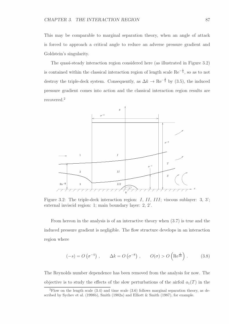
CHAPTER 3. THE INTERACTION REGION 87
This may be comparable to marginal separation theory, when an angle of attack
is forced to approach a critical angle to reduce an adverse pressure gradient and
Goldstein’s singularity.
The quasi-steady interaction region considered here (as illustrated in Figure 3.2)
is contained within the classical interaction region of length scale Re−15 , so as to not
destroy the triple-deck system. Consequently, as ∆k → Re−25 by (3.5), the induced
pressure gradient comes into action and the classical interaction region results are
recovered.2
1
2
2’
3’
0
III
II
I
σ−4
y
Re−12 3
σ−1
σ−4
x
Figure 3.2: The triple-deck interaction region: I, II, III; viscous sublayer: 3, 3’;external inviscid region: 1; main boundary layer: 2, 2’.
From hereon in the analysis is of an interactive theory when (3.7) is true and the
induced pressure gradient is negligible. The flow structure develops in an interaction
region where
(−s) = O(
σ−4)
, ∆k = O(
σ−8)
, O(σ) > O(
Re120
)
. (3.8)
The Reynolds number dependence has been removed from the analysis for now. The
objective is to study the effects of the slow perturbations of the airfoil a1(T ) in the
2Flow on the length scale (3.4) and time scale (3.6) follows marginal separation theory, as de-scribed by Sychev et al. (1998b), Smith (1982a) and Elliott & Smith (1987), for example.
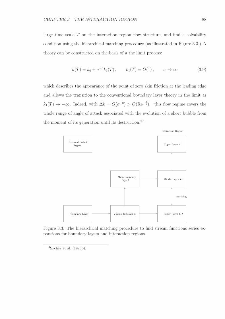
CHAPTER 3. THE INTERACTION REGION 88
large time scale T on the interaction region flow structure, and find a solvability
condition using the hierarchical matching procedure (as illustrated in Figure 3.3.) A
theory can be constructed on the basis of a the limit process:
k(T ) = k0 + σ−8k1(T ) , k1(T ) = O(1) , σ →∞ (3.9)
which describes the appearance of the point of zero skin friction at the leading edge
and allows the transition to the conventional boundary layer theory in the limit as
k1(T ) → −∞. Indeed, with ∆k = O(σ−8) > O(Re−25 ), “this flow regime covers the
whole range of angle of attack associated with the evolution of a short bubble from
the moment of its generation until its destruction.”3
Layer 2
Region
Boundary Layer
Main Boundary
matching
Viscous Sublayer 3
External Inviscid
Interaction Region
Lower Layer III
Middle Layer II
Upper Layer I
Figure 3.3: The hierarchical matching procedure to find stream functions series ex-pansions for boundary layers and interaction regions.
3Sychev et al. (1998b).
CHAPTER 3. THE INTERACTION REGION 89
3.2 The Middle Layer
The middle layer (region II in Figure 3.2) of the interaction region continues from
the main boundary layer (region 2) and has a similar limit process:
s∗ = x∗ − xs = σ4s = O(1) , Y = O(1) , σ →∞ . (3.10)
The main boundary layer stream function (2.81) in middle layer variables (3.9) and
(3.10), is:
Ψ =1
6λ0Y
3 +
σ−4s∗[
1
2a0Y
2 − 1
2 · 5!a20Y
5 + . . .
]
+ . . .
+ σ−8k1
σ4s∗−11
2a1Y
2 + . . .
+ . . .
that is
Ψ =1
6λ0Y
3 + σ−4
s∗[
1
2a0Y
2 − 1
2 · 5!a20Y
5 + . . .
]
+ k1s∗−11
2a1Y
2 + . . .
+ . . .
Hence, the middle layer stream function is assumed to be of the form:
Ψ = Ψ00(Y ) + σ−4Ψ∗1(x
∗, Y, T ) + . . . Ψ00(Y ) =1
6λ0Y
3 (3.11)
and the condition of matching with the main boundary layer is
Ψ∗1(x
∗, Y, T ) = s∗[
1
2a0Y
2 − 1
2 · 5!a20Y
5 + . . .
]
+ k1s∗−11
2a1Y
2 + . . . (3.12)
s∗ → −∞ .
The middle layer equation, from the boundary layer equation (2.14) with (3.10), is:
1
σ
∂2Ψ
∂T∂Y+ σ4 ∂Ψ
∂Y
∂2Ψ
∂x∗∂Y− σ4 ∂Ψ
∂x∗∂2Ψ
∂Y 2=∂3Ψ
∂Y 3− σ4 ∂p
∂x∗.
CHAPTER 3. THE INTERACTION REGION 90
The pressure gradient is the superposition of the original Taylor series expansion
(2.15) and the induced pressure gradient: ∂P ∗
∂x∗, from (3.3):
σ4 ∂p
∂x∗= λ0 + σ−4s∗λ1 + . . .+ Re−
12σ4∂P
∗
∂x∗+ . . . (3.13)
Recall that the induced pressure gradient is negligible in this regime with scales (3.8).
Substituting (3.11) and (3.13) into the middle layer equation, and gathering the
O(1) terms, gives the Ψ∗1(x
∗, Y, T ) equation:
∂Ψ00
∂Y
∂2Ψ∗1
∂x∗∂Y− ∂2Ψ00
∂Y 2
∂Ψ∗1
∂x∗=∂3Ψ00
∂Y 3− λ0 .
Rearranging the Ψ∗1(x
∗, Y, T ) equation gives a solution for Ψ∗1(x
∗, Y, T ) in the form:
Ψ∗1 = Ψ′
00
A1(x∗, T )
λ0+ s∗
Y∫
0
Ψ′′′00 − λ0(Ψ′
00)2
dY
(3.14)
where, by (3.11):
Ψ00(Y ) =1
6λ0Y
3 . (3.15)
The A1(x∗, T ) term is arbitrary except the condition of matching (3.12) to the main
boundary layer requires that
A1(x∗, T ) = k1s
∗−1a1 + s∗[
a0 −1
5!a0Y
3 + . . .
]
+ . . . s∗ → 0 (3.16)
Moreover, substituting the middle layer stream function (3.11) and the pressure
gradient (3.13) into the second, y-momentum equation (1.2) for the boundary layer
then gathering O(Re12 ) terms, gives:
∂p
∂Y= 0 .
CHAPTER 3. THE INTERACTION REGION 91
Differentiating with respect to x∗ indicates that
∂
∂Y
(
∂P ∗
∂x∗
)
= 0 . (3.17)
The induced pressure gradient, although negligible in this regime, would remain un-
changed across the middle layer of the classical interaction region.
3.3 The Lower Layer
The lower layer (region III in Figure 3.2) of the interaction region continues from
the viscous sublayer (region 3) and hence, has the limit process:
s∗ = x∗ − xs = σ4s = O(1) , Y ∗ = σY = O(1) , η∗ =Y ∗
(s∗)14
, σ →∞ . (3.18)
The viscous sublayer stream function (2.77) in lower layer variables (3.9) and (3.18),
is:
Ψ =
σ−3 1
6λ0Y
∗3 + σ−6s∗321
2a0η
∗2 + . . .
+ σ−9s∗94
[
1
2b0η
∗2 − 1
5!a20η
∗5 +1
8!λ0a
20η
∗9
]
+ . . .
+ σ−8k1
σ2s∗−121
2a1η
∗2 + σ−1s∗141
2b1η
∗2 + . . .
+ σ−9k1
1
2b2η
∗2 + . . .
+ . . .
CHAPTER 3. THE INTERACTION REGION 92
that is
Ψ = σ−31
6λ0Y
∗3 + σ−6
s∗1
2a0Y
∗2 + k1s∗−1 1
2a1Y
∗2 + . . .
+ σ−9
s∗741
2b0Y
∗2 − s∗ 15!a20Y
∗5 +1
8!λ0a
20Y
∗9
+ s∗−14k1
1
2b1Y
∗2 + s∗−12k1
1
2b2Y
∗2 + . . .
+ . . . (3.19)
Hence, the lower layer stream function is assumed to be of the form:
Ψ = σ−3Ψ∗00(Y
∗) + σ−6Ψ∗1(x
∗, Y ∗, T ) + σ−9Ψ∗2(x
∗, Y ∗, T ) + . . . (3.20)
Ψ∗00 =
1
6λ0Y
∗3
The lower layer equation, from the boundary layer equation (2.14) with (3.18), is:
∂2Ψ
∂T∂Y ∗+ σ6 ∂Ψ
∂Y ∗
∂2Ψ
∂x∗∂Y ∗− σ6 ∂Ψ
∂x∗∂2Ψ
∂Y ∗2= σ3 ∂
3Ψ
∂Y ∗3− σ4 ∂p
∂x∗
3.3.1 Ψ∗1(x∗, Y ∗, T ) Solution
Substituting (3.20) and pressure gradient (3.13) into the lower layer equation, and
gathering the O(σ−3) terms, gives the Ψ∗1 equation:
1
2λ0Y
∗2 ∂2Ψ∗1
∂x∗∂Y ∗− λ0Y ∗2∂Ψ
∗1
∂x∗=∂3Ψ∗
1
∂Y ∗3. (3.21)
The boundary conditions are
Ψ∗1 =
∂Ψ∗1
∂Y ∗= 0 , Y ∗ = 0 . (3.22)
CHAPTER 3. THE INTERACTION REGION 93
The condition of matching with the middle layer (region II) and the viscous sublayer
(region 3) is that
Ψ∗1 =
1
2A1(x
∗, T )Y ∗2 + . . . Y ∗ →∞ , x∗ → −∞ . (3.23)
The solution of the boundary value problem (3.21), (3.22), (3.23) is:
Ψ∗1 =
1
2A1(x
∗, T )Y ∗2 , (3.24)
where the function A1(x∗, T ) remains arbitrary in this layer.
3.3.2 Ψ∗2(x∗, Y ∗, T ) Solution & the A1(x
∗, T ) Function
To determine the function A1(x∗, T ), the Ψ∗
2 boundary value problem must also be
considered. The Ψ∗2 equation is sought in a similar way to (3.21) but comes from
collecting the O(σ−6) terms instead. The Ψ∗2 equation is
∂A1
∂TY ∗ +
1
2A1∂A1
∂x∗Y ∗2 +
1
2λ0Y
∗2 ∂2Ψ∗2
∂x∗∂Y ∗− λ0Y ∗∂Ψ
∗2
∂x∗=∂3Ψ∗
2
∂Y ∗3. (3.25)
The induced pressure gradient from (3.13): ∂P ∗
∂x∗, does not balance with the O(σ−6)
terms since O(σ−6) > O(Re−12σ4), as discussed in Section 3.1. The boundary condi-
tions are
Ψ∗2 =
∂Ψ∗2
∂Y ∗= 0 , Y ∗ = 0 . (3.26)
The condition of matching with the viscous sublayer (3.19) is
Ψ∗2 =
1
8!λ0a
20Y
∗9 + s∗1
5!a20Y
∗5 +1
2A2(x
∗, T )Y ∗2 + . . . x∗ → −∞
where
A2 = s∗74 b0 + s∗−
14 b1 + s∗−
24 b2 + . . . = O(s∗
74 ) , x∗ → −∞ . (3.27)
CHAPTER 3. THE INTERACTION REGION 94
The condition of matching with the middle layer (3.14) and (3.16), is constructed so
that it is of the same order of magnitude as (3.27). By (3.16):
A21 − x∗2a20 − 2k1a0a1 = x∗−2k21a
21 + . . . = O(s∗−2)
and by the similarity variable (3.18): Y ∗ = O(s∗14 ). Hence, the condition of matching
with the middle layer is
Ψ∗2 =
1
2λ0
[
A21(x
∗, T )− a20x∗2 − 2k1a0a1]
Y ∗ + . . . = O(s∗74 ) , Y ∗ →∞
The combined condition of matching to the viscous sublayer and middle layer is:
Ψ∗2 =
1
8!λ0a
20Y
∗9 + s∗1
5!a20Y
∗5 +1
2A2(x
∗, T )Y ∗2
+1
2λ0
[
A21(x
∗, T )− a20x∗2 − 2k1a0a1]
Y ∗ + o(1) ,
Y ∗ →∞ , x∗ → −∞ (3.28)
with A2(x∗, T ) (3.27).4 The A1(x
∗, T ) function is to be determined.
A Change Of Variable & Affine Transformation
Analogous to Ruban (1982b), a change of variable:
Ψ∗2 = Ψ2 +
λ08!a20Y
∗9 +1
5!a20x
∗Y ∗5 +1
2λ0
[
A21 − a20x∗2 − 2k1a0a1
]
Y ∗
is made, to simplify the problem. The Ψ∗2 equation (3.25) becomes:
∂A1
∂TY ∗ +
1
2λ0Y
∗2 ∂2Ψ2
∂x∗∂Y ∗− λ0Y ∗∂Ψ2
∂x∗=∂3Ψ2
∂Y ∗3
4Ruban (1982a)
CHAPTER 3. THE INTERACTION REGION 95
with the boundary conditions (3.26):
Ψ2 = 0 ,∂Ψ2
∂Y ∗=
1
2λ0
[
A21 − a20x∗2 − 2k1a0a1
]
, Y ∗ = 0
and condition of matching (3.28):
Ψ2 =1
2A2(x
∗, T )Y ∗2 , Y ∗ →∞ , x∗ → −∞ .
Next, the affine transformations:
Ψ2 = a11100 U
9500λ
− 1710
0 Ψ2 , x∗ = a− 2
50 U
4500λ
− 15
0 x , T = a− 9
100 U
− 15
00 λ3100 T ,
y∗ = a− 1
100 U
1500λ
− 310
0 y , A1 = a350U
4500λ
− 15
0 A1 , a = k1(−a1)a− 1
50 U
− 85
00 λ250 (3.29)
are applied, to reduce the number of parameters in the system. The equation be-
comes:
1
2Y 2 ∂
2Ψ2
∂x∂Y− Y ∂Ψ2
∂x=∂3Ψ2
∂Y 3− ∂A1
∂TY (3.30)
with the boundary conditions:
Ψ2 = 0 ,∂Ψ2
∂Y= g(x, T ) = −1
2
(
A21 − x2 + 2a
)
, Y = 0 (3.31)
and the conditions of matching to the middle layer and viscous sublayer:
Ψ2 = O(Y 2) , Y →∞ ; Ψ2 = o(1) , x→ −∞ . (3.32)
3.3.3 The Fourier Transformation Boundary Value Problem
A Fourier transformation is applied to the boundary value problem (3.30), (3.31) and
(3.32), where by definition:
Φ(k, Y , T ) =1√2π
∞∫
−∞
Ψ2(x, Y , T )e−ikx dx .
CHAPTER 3. THE INTERACTION REGION 96
Hence, the equation becomes
d3Φ
dY 3− 1
2ikY 2 dΦ
dY+ ikY Φ = Y R(k, T ) , (3.33)
where R(k, T ) is the Fourier transform of ∂A1
∂Tsuch that
R(k, T ) =1√2π
∞∫
−∞
∂A1
∂T(x, T )eikx dx .
The boundary conditions become
Φ = 0 ;dΦ
dY= G(k, T ) , Y = 0 , (3.34)
where G(k, T ) is the Fourier transform of g(x, T ) such that
G(k, T ) =1√2π
∞∫
−∞
g(x, T )eikx dx .
The condition of matching is
Φ = O(1) , Y →∞ . (3.35)
The general solution of the problem (3.33), (3.34) and (3.35) is
Φ = C1Φ1 + C2Φ2 + C3Φ3 +R(k, T )Φ∗ ,
where Φ1(Y , T ), Φ2(Y , T ), Φ3(Y , T ) are complimentary solutions of the homogeneous
equation and Φ∗(Y , T ) is the particular integral.
Complimentary Solutions
The complimentary solutions Φ1, Φ2 and Φ3 are linearly independent solutions of
the homogeneous form of (3.33). They can be chosen so that their Taylor series
CHAPTER 3. THE INTERACTION REGION 97
expansions about the point Y = 0 begin with 1, Y or Y 2, respectively. The boundary
conditions at Y = 0:
Φ1 = 1 ,dΦ1
dY= 0 ,
d2Φ1
dY 2= 0 ;
Φ2 = 0 ,dΦ2
dY= 1 ,
d2Φ2
dY 2= 0 ; (3.36)
Φ3 = 0 ,dΦ3
dY= 0 ,
d2Φ3
dY 2= 1
require that
C1 = 0 , C2 = G(k, T ) , C3 = C (3.37)
where C is an arbitrary constant. Indeed, by observation:
Φ3 =1
2Y 2 .
The complimentary solution Φ2(Y , T ) may be found using the Frobenius method:
Φ2 =
∞∑
m=0
Dm(T )Y4m+β , D0(T ) 6= 0
where Dm(T ) are functions of time to be found from initial conditions. For m = 0:
dΦ2
dY= D0βY
β−1 = 1⇒ D0 = 1 , β = 1
by the boundary conditions (3.36). Upon substitution into homogeneous form of
(3.33), then:
∞∑
m=0
Dm(4m+ 1)(4m)(4m− 1)Y 4m−2 − 1
2ik
∞∑
m=1
Dm−1(4m− 5)Y 4m−2 = 0 .
For m = 0, there is the trivially true: D0 · 0 = 0.
CHAPTER 3. THE INTERACTION REGION 98
For all m ≥ 1, there is the recurrence relation for Dm(T ):
Dm =
(
ik
32
)
(m− 54)
(m+ 14)(m)(m− 1
4)Dm−1 , D0 = 1 .
For example, for m = 1:
D1 =
(
ik
32
) −14
54· 34
.
The functions for m ≥ 1 can be written:
Dm = −Γ(
5
4
)(
ik
32
)m1
m! · Γ(m+ 14+ 1) · (4m− 1)
.
Hence, the complimentary solution is:5
Φ2 = Y − Γ
(
5
4
) ∞∑
m=1
(
ik
32
)m1
m! · Γ(m+ 14+ 1) · (4m− 1)
Y 4m+1 ,
or, in terms of Bessel functions of the first kind:
Φ2 = −2Γ(5
4)
Ω14 e
iπ4
− 1
Γ(54)
(
ξ
2
)12
+ξ
8
ξ∫
0
(
ξ12
)− 32
[
(
ξ12
)− 14
J 14(ξ1)−
1
Γ(54)
]
dξ1
(3.38)
where
Ω =ik
2, ξ =
iΩ12 Y 2
2. (3.39)
Bessel functions of the first kind are defined in Section 3.3.4.
Particular Solution
A particular solution of (3.33) which satisfies the condition of matching (3.35) can
be determined from observation:
Φ∗ =1
ik,
5Ruban (1982a)
CHAPTER 3. THE INTERACTION REGION 99
which is also the first term in an asymptotic series solution. Analogous to the Frobe-
nius method for finding the complimentary solution (3.38), the particular solution,
in terms of Bessel functions of the first kind, is:6
Φ∗ =Γ(3
4)
4Ω
(
ξ
2
)
ξ∫
0
(
ξ12
)− 74
[
J− 14(ξ1)−
1
Γ(34)
(
ξ12
)− 14
]
dξ1 (3.40)
with Ω and ξ as (3.39).
3.3.4 Bessel Functions of the First Kind
The Bessel function of the first kind is defined7 for fixed real parameter ν (which is
not to be confused with the kinematic viscosity in Chapter 1) and real z ≥ 0, as:
Jν(z) =
∞∑
m=0
(−1)mm! · Γ(m+ ν + 1)
(
1
2|z|2m+ν
)
. (3.41)
The behaviour of (3.41) for ν = ±14ensures that the complimentary (3.38) and
particular (3.40) solutions converge to finite values as ξ → 0.
Furthermore, as z →∞, the Bessel function of the first kind behaves like:
Jν(z) =
√
2
(πz)
cos
(
z − 1
2νπ − 1
4π
)
+ e|∮z|O(
|z|−1)
, | arg z| < π . (3.42)
6Ruban (1982a)7See for example, Abramovich & Stegun (1972).
CHAPTER 3. THE INTERACTION REGION 100
3.3.5 General Solution
To summarise, the general solution of the boundary value problem (3.33), (3.34) and
(3.35) is
Φ =1
2CY 2
−G · 2Γ(54)
Ω14 e
iπ4
− 1
Γ(54)
(
ξ
2
)12
+ξ
8
ξ∫
0
(
ξ12
)− 32
[
(
ξ12
)− 14
J 14(ξ1)−
1
Γ(54)
]
dξ1
+R · Γ(34)
4Ω
(
ξ
2
)
ξ∫
0
(
ξ12
)− 74
[
J− 14(ξ1)−
1
Γ(34)
(
ξ12
)− 14
]
dξ1 (3.43)
where (3.39):
Ω =ik
2, ξ =
iΩ12 Y 2
2.
Matching At The Outer Lower Layer
As the outer edge of the lower layer is approached and ξ → ∞ then by (3.42), the
complimentary solution (3.38) changes to
Φ2 = −Γ(5
4)
2√πΩ
14 e
iπ4
(
ξ
2
)− 54
sin
(
ξ − 3
8π
)
+ . . .
and the particular solution (3.40) becomes
Φ∗ =Γ(3
4)
4√πΩ
(
ξ
2
)− 54
sin
(
ξ − 1
8π
)
+ . . .
CHAPTER 3. THE INTERACTION REGION 101
Hence, as ξ →∞, the lower layer general solution (3.43) behaves like
Φ =1
2CY 2
−G · Γ(54)
2√πΩ
14
(
ξ
2
)− 54
e−iπ4 sin
(
ξ − 3
8π
)
+R · Γ(34)
4√πΩ
(
ξ
2
)− 54
sin
(
ξ − 1
8π
)
+ . . .
The trigonometric terms sin(
ξ − 38π)
and sin(
ξ − 18π)
behave like complex hyperbolic
functions since ξ (3.39) is complex. As ξ →∞, they grow unbounded. The condition
of no exponential growth as ξ →∞ is satisfied when:8
R(k, T )(ik)−34 = G(k, T )
Γ(54)
Γ(34)2
14 (3.44)
and the trigonometric terms are removed. The relation (3.44) completes the matching
between the lower layer and the middle layer. When true, the interaction region flow
structure, with a negligible induced pressure gradient, is consistent.
3.3.6 The A(x, T ) Solvability Condition from Inverse Fourier
Transformation
Recall from (3.33) and (3.34) that R(k, T ) and G(k, T ) are the Fourier transforms of
∂A1
∂T(x, T ) and g(x, T ) = −1
2
(
A21 − x2 + 2a
)
. Applying the inverse Fourier transfor-
mation to (3.44) results in:
1√2π
∞∫
−∞
R(k, T )(ik)−34 eixk dk =
[
Γ(54)
Γ(34)2
14
]
1√2π
∞∫
−∞
G(k, T )eixk dk (3.45)
8A similar result for marginal separation with induced pressure gradient is found by Ruban(1982b). See also Samad (2004) and Stavrou (2004).
CHAPTER 3. THE INTERACTION REGION 102
and hence:9
[
Γ(54)
Γ(34)2
14
]
g(x, T ) =1
2π
x∫
−∞
dξ
∞∫
−∞
∂A1
∂T(ξ, T )(ik)−
34 ei(x−ξ)k dk .
By rewriting (x− ξ) = p, then:
[
Γ(54)
Γ(34)2
14
]
g(x, T ) =1
2π
x∫
−∞
∂A1
∂T(ξ, T )
∞∫
−∞
(ik)−34 eipk dk
dξ .
Let the integral:10
I =
∞∫
−∞
(ik)−34 eipk dk .
In the k-plane, as illustrated in Figure 3.4:
eipk = eip(kr+iki) = e−pkieipkr .
For all p > 0, the contour of integration may be closed in the upper-half k-plane with
a branch cut along the positive imaginary axis. Therefore,
I =
∮
C1
−∫
C11
−∫
C12
+
∮
C2
−∫
C21
−∫
C22
(ik)−34 eipk dk .
Cauchy’s residue theorem states:
∮
C
f(k) dk = 2πi
n∑
j=1
Res(f, aj)
where
1. the contour C is a simple closed curve in the anti-clockwise direction;
2. the term Res(f, aj) denotes the residue of f at the point k = aj for j =
9The integral term ξ is not the parameter ξ from the Fourier transform boundary value problemsolution in Section 3.3.3 of the lower layer analysis.
10See also work by Samad (2004) and Stavrou (2004).
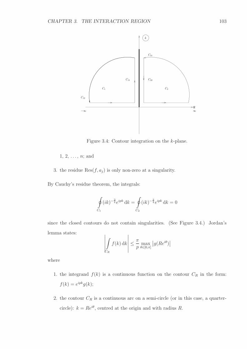
CHAPTER 3. THE INTERACTION REGION 103
−∞
C2C1
C12
C22C11
C21
k
∞ℜ
Figure 3.4: Contour integration on the k-plane.
1, 2, . . . , n; and
3. the residue Res(f, aj) is only non-zero at a singularity.
By Cauchy’s residue theorem, the integrals:
∮
C1
(ik)−34 eipk dk =
∮
C2
(ik)−34 eipk dk = 0
since the closed contours do not contain singularities. (See Figure 3.4.) Jordan’s
lemma states:∣
∣
∣
∣
∣
∣
∫
CR
f(k) dk
∣
∣
∣
∣
∣
∣
≤ π
pmaxθ∈[0,π]
∣
∣g(Reiθ)∣
∣
where
1. the integrand f(k) is a continuous function on the contour CR in the form:
f(k) = eipkg(k);
2. the contour CR is a continuous arc on a semi-circle (or in this case, a quarter-
circle): k = Reiθ, centred at the origin and with radius R.
CHAPTER 3. THE INTERACTION REGION 104
By Jordan’s lemma, the upper bound of the integral on the quarter-circle arc C12:
∣
∣
∣
∣
∣
∣
∫
C12
(ik)−34 eipk dk
∣
∣
∣
∣
∣
∣
≤ π
2pmax
θ∈[π2 ,π]
∣
∣
∣
(
iReiθ)− 3
4
∣
∣
∣→ 0 , R→∞ .
Analogously, the integral on the quarter-circle arc: C21 = 0.
For all p < 0 where the integration is performed in the lower-half k-plane, the
integrand is analytic and the contribution to the integral is also zero.
The remaining non-zero integrals are therefore:
I =
−∫
C11
−∫
C22
(ik)−34 eipk dk ,
of which∞∫
0
(ik)−34 eipk dk = −
∫
C22
(ik)−34 eipk dk , (3.46)
0∫
−∞
(ik)−34 eipk dk = −
∫
C11
(ik)−34 eipk dk . (3.47)
For (3.46), the contour can be parameterized by:
k = eiπ2 y = iy ;
hence∞∫
0
(ik)−34 eipk dk = e−iπ
4
∞∫
0
y−34 e−py dy ,
and with a change of variable from y to t such that y =(
1p
)
t, then:
∞∫
0
(ik)−34 eipk dk = e−iπ
4 p−14
∞∫
0
t−34 e−t dt .
CHAPTER 3. THE INTERACTION REGION 105
By definition of the Gamma function (2.29), then
∞∫
0
(ik)−34 eipk dk = e−iπ
4 p−14Γ
(
1
4
)
.
Analogously, for (3.47):
0∫
−∞
(ik)−34 eipk dk = e−i 3π
4 p−14Γ
(
1
4
)
.
Therefore, the integral is
I =
√πΓ(
14
)
(x− s) 14
.
Overall, (3.45) with integral I is
A21(x, T )− x2 + 2a = − 2
34
Γ(54)
x∫
−∞
∂A1
∂T(ξ, T )
dξ
(x− ξ) 14
. (3.48)
The A1(x, T ) equation (3.48) is the necessary and sufficient solvability condition for
the interaction region flow structure, with a negligible induced pressure gradient, to
be consistent and hence, for solutions to exist. The solvability condition is a result
of the condition of matching (3.28) between the middle layer and the lower layer of
the interaction region; a change of variables and affine transformation (3.29); the
subsequent Fourier transformation boundary value problem in Section 3.3.3; and the
inverse Fourier transformation of the condition (3.45). It is a part of the hierarchical
process for determining stream functions by region, as illustrated in Figure 3.3.
Abel Integral Transformation of the A(x, T ) Solvability Condition
The Abel integral transform for a “sufficiently well behaved function u” is
f(x) =1
Γ(α)
x∫
a
(x− t)α−1u(t) dt
CHAPTER 3. THE INTERACTION REGION 106
for a < x < b, −∞ ≤ a < b ≤ ∞ and real α ∈ (0, 1).11 The inverse Abel integral
transform for a sufficiently well behaved f(x) is
u(x) =1
Γ(1− α)d
dx
x∫
a
(x− t)−αf(t) dt .
Hence, the solvability condition (3.48) may be transformed to the conservative form:
∂A1
∂T(x, T ) = −Γ(
54)
254π
∂
∂x
x∫
−∞
[
A21(s, T )− s2 + 2a(T )
] ds
(x− s) 34
, (3.49)
with use of the Gamma multiplication theorem:
Γ(z)Γ(
z +1
2
)
= 21−2z√πΓ(2z) ,
and properties of the Gamma function (2.29).
Induced Pressure Gradient Discussion
Recall that if the induced pressure gradient is not negligible in this regime, then it
remains unchanged across the middle layer, as discussed in Section 3.2.
Substituting the lower layer stream function (3.20) and the pressure gradient
(3.13) into the second, y-momentum equation (1.2) for the boundary layer then gath-
ering O(Re12σ) terms, gives:
∂p
∂Y ∗= 0 .
Differentiating with respect to x∗ indicates that
∂
∂Y ∗
(
∂P ∗
∂x∗
)
= 0 .
The induced pressure gradient, although negligible in this regime, would remain un-
changed across the lower layer as well as the middle layer.
11Gorenflo & Vessella (2008)
CHAPTER 3. THE INTERACTION REGION 107
3.4 The Upper Layer
The interaction region problem is closed, with the derivation of the A(x, T ) solvability
condition (3.48), because the induced pressure gradient is negligible. In other words,
there is no need to consider an upper layer (region I in Figure 3.2) of the traditional
triple deck theory for the interaction region.
In contrast, if the induced pressure gradient is not negligible, the ∂P ∗
∂x∗term appears
in the Ψ∗2 equation (3.25) of the lower layer analysis. The induced pressure gradient
then remains undetermined in the lower layer analysis and to close the interaction
region problem, it is necessary to consider the upper layer. The induced pressure
gradient of the lower layer causes a displacement effect of the boundary layer in the
upper layer.
A relationship between the pressure and displacement can be obtained by consid-
ering the classical triple deck interaction region flow regime. The induced pressure
gradient is determined by the curvature of the streamlines in the lower layer adjacent
to the wall and the integral of small perturbation theory (B.6).12
The curvature of the lower layer streamlines can be found from matching with
the middle layer stream function solution (3.11) and (3.14). In the middle layer,
u = Ψ′00(Y ) + . . .
v = −Re− 12Ψ′
00(Y )
A′1(x
∗)
λ0+
Y∫
0
Ψ′′′00 − λ0(Ψ′
00)2
dY
+ . . .
Therefore, the angle of inclination of the velocity vector is
θ =v
u= −Re− 1
2
A′1(x
∗)
λ0+
Y∫
0
Ψ′′′00 − λ0(Ψ′
00)2
dY
+ . . .
12The integral of small perturbation theory is derived in Appendix B.
CHAPTER 3. THE INTERACTION REGION 108
and the curvature of the streamlines is
∂θ
∂x= Re−
12σ−4A
′′1(x
∗)
λ0.
As σ → Re120 by (3.7), the induced pressure gradient becomes significant to the
flow regime and the classical triple deck interaction region comes into action. When
the curvature of the streamlines is substituted into the integral of small perturbation
theory, then the pressure-displacement relation is obtained:
∂P ∗
∂x∗= − U2
0
πλ0−∞∫
−∞
A′′1(ξ)
ξ − x∗ dξ . (3.50)
The pressure-displacement relation closes the interaction region problem when an
induced pressure gradient is present in the flow. It relates the displacement effect of
the boundary layer to the induced pressure gradient.
Chapter 4
A(x, T ) Solvability Condition
Analysis
The construction of the initial-boundary value problem for the solvability condition
(3.48) for the interaction region:
A2(x, T )− x2 + 2a(T ) = − 234
Γ(54)
x∫
−∞
∂A
∂T(ξ, T )
dξ
(x− ξ) 14
(4.1)
and its numerical solution, based on the methods set out by Smith & Elliott (1985),
follows. For simplicity, the bar and subscript notation is removed.
The A(x, T ) term originates from the perturbation solution (3.24):
Ψ∗1 =
1
2A1(x
∗, T )Y ∗2
of the lower layer (region III) stream function (3.20), where it has been manipulated
by the affine transformation (3.29):
A1 = a350U
4500λ
− 15
0 A1 , A1 = A .
109
CHAPTER 4. A(X, T ) SOLVABILITY CONDITION ANALYSIS 110
Hence, the A(x, T ) term is directly proportional to the skin friction, defined as
τ =∂2Ψ
∂Y 2
∣
∣
∣
∣
Y=0
= A(x, T ) + . . . (4.2)
If skin friction is positive then the fluid flow is attached and moving downstream. If
skin friction is negative the flow is moving upstream against the current. Steady flow
separation is deemed to have occurred when skin friction equals zero. Unsteady flow
separation occurs at a point of zero skin friction and zero velocity.
The parameter a(T ) also comes from the affine transformation (3.29):
a = k1(−a1)a− 1
50 U
− 85
00 λ250 .
The function k1(T ) comes from the interaction region asymmetry function (3.9):
k(T ) = k0 + σ−8k1(T ), as σ → ∞. The parameter a1(T ) ∼ ∆k is related to the
change in angle of attack and comes from the first eigenvalue of the viscous sublayer
stream function perturbation Ψ1(x, Y, T ). Its rate of change: a1(T ), which is related
to the rate of change of angle of attack, also appears in the forcing term Ψ2(x, Y, T ).
In classic steady marginal separation theory, skin friction A solutions exist for
large negative values of a up to a critical value ac = 1.33. For larger values of a, no
flow solutions can be obtained, or to be more precise, solutions becomes complex.1
For an airfoil with a slow change in angle of attack on the large time scale T then
a(T ) can be set to sweep through a range of values over some time range T ≥ 0.
Moreover, for an airfoil close to stall then a(T ) can be set to start close to but below
the critical value ac = 1.33, which then gently approaches the point of no real solution
at a = ac. For example:
a(T ) = 1.331− (1.331 + 0.001)e−T , T ≥ 0 , (4.3)
1c.f. Stewartson et al. (1982) and the review by Sychev et al. (1998b) on marginal separation, inSection 1.4.
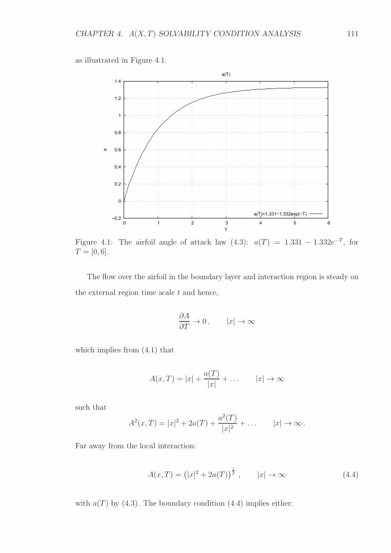
CHAPTER 4. A(X, T ) SOLVABILITY CONDITION ANALYSIS 111
as illustrated in Figure 4.1.
−0.2
0
0.2
0.4
0.6
0.8
1
1.2
1.4
0 1 2 3 4 5 6
a
T
a(T)
a(T)=1.331−1.332exp(−T)
Figure 4.1: The airfoil angle of attack law (4.3): a(T ) = 1.331 − 1.332e−T , forT = [0, 6].
The flow over the airfoil in the boundary layer and interaction region is steady on
the external region time scale t and hence,
∂A
∂T→ 0 , |x| → ∞
which implies from (4.1) that
A(x, T ) = |x|+ a(T )
|x| + . . . |x| → ∞
such that
A2(x, T ) = |x|2 + 2a(T ) +a2(T )
|x|2 + . . . |x| → ∞ .
Far away from the local interaction:
A(x, T ) =(
|x|2 + 2a(T )) 1
2 , |x| → ∞ (4.4)
with a(T ) by (4.3). The boundary condition (4.4) implies either:
CHAPTER 4. A(X, T ) SOLVABILITY CONDITION ANALYSIS 112
1. the flow is attached to the surface; the skin friction is positive far away from
the local interaction such that
A(x, T ) =∣
∣
∣
(
|x|2 + 2a(T ))
12
∣
∣
∣, |x| → ∞
(c.f. the boundary condition (1.7) from Ryzhov & Smith (1984) and Stewartson
et al. (1982) on marginal separation), or
2. the flow direction is reversed far away from the interaction region and the
negative root is taken such that
A(x, T ) = −∣
∣
∣
(
|x|2 + 2a(T ))
12
∣
∣
∣, |x| → ∞
(c.f. the boundary condition (1.8) from Ryzhov & Smith (1984) and Brown &
Stewartson (1983)).
The thesis follows the theory of marginal separation from Stewartson et al. (1982).
Hence, the class of far away attached flows is considered and the positive root of the
boundary condition (4.4) is taken. Boundary conditions are important here because if
they are not imposed, the solution is not unique. For example, if a = 0, the solvability
condition (4.1) allows two solutions A = x and A = −x besides the solution(s) that
meets the condition.
Initial conditions at T = 0: A(x, 0), are discussed in Section 4.4.1.
4.1 A(x, T ) Equation Numerical Treatment
Solutions for the A(x, T ) equation (4.1):
A2(x, T )− x2 + 2a(T ) = − 234
Γ(54)
x∫
−∞
∂A
∂T(ξ, T )
dξ
(x− ξ) 14
CHAPTER 4. A(X, T ) SOLVABILITY CONDITION ANALYSIS 113
are found based on the following numerical treatment described by Smith & Elliott
(1985). This numerical treatment is chosen because Smith & Elliott use the method
to acquire solutions for a normalised quasi-steady version (4.5) of (4.1) where 2a(T )
is a constant Γ:
A2(x, T )− x2 + Γ =
x∫
−∞
∂A
∂T(ξ, T )
dξ
(x− ξ) 14
. (4.5)
The Smith & Elliott (1985) equation (4.5) is derived in a similar manner to (4.1).2
The treatment is tested in the Sections 4.3 and 4.4.
Equation (4.1) is to be reformulated as a system of nonlinear equations on a
uniform space x and time T grid. (See Figure 4.2.) Ultimately, the nonlinear system of
equations will be solved numerically using Newton’s method described in Section 4.2.
The computational spatial x-range is finite. It is discretised with a uniform step
size Dx into m+ 1 grid points, where x1 is the large and negative (but not negative
infinity) starting point of the computational domain; xm+1 is the large and positive
end point; and the subscript i denotes evaluation at an internal grid point xi =
x1 + (i − 1)Dx for i = 1, 2, . . . , m + 1. There are m steps from x1 to xm+1. The
notation Ai denotes A(xi, T ).
The forward time T -range is similarly discretised with a uniform step size DT into
n+1 grid points where the time steps are Tk = T1+(k−1)DT for k = 1, 2, . . . , n+1.3
There are n steps from T1 to Tn+1.
If k = 1 and T = 0, then the value A(0)i at all xi for i = 1, 2, . . . , m+ 1 is known
from an initial condition given in Section 4.4.1. The solutions A1 and Am+1 for all
time T are known from boundary conditions (4.4), now reformulated as
A(x, T ) =(
|x|2 + 2a(T ))
12 ; x = x1, xm+1 ; ∀T . (4.6)
Furthermore, the superscripts (0) and (1) are introduced to denote iteration levels
2See also Smith (1982a).3The start point T1 = 0 has subscript 1 and not 0 because it denotes the first entry into a vector
in MATLAB.
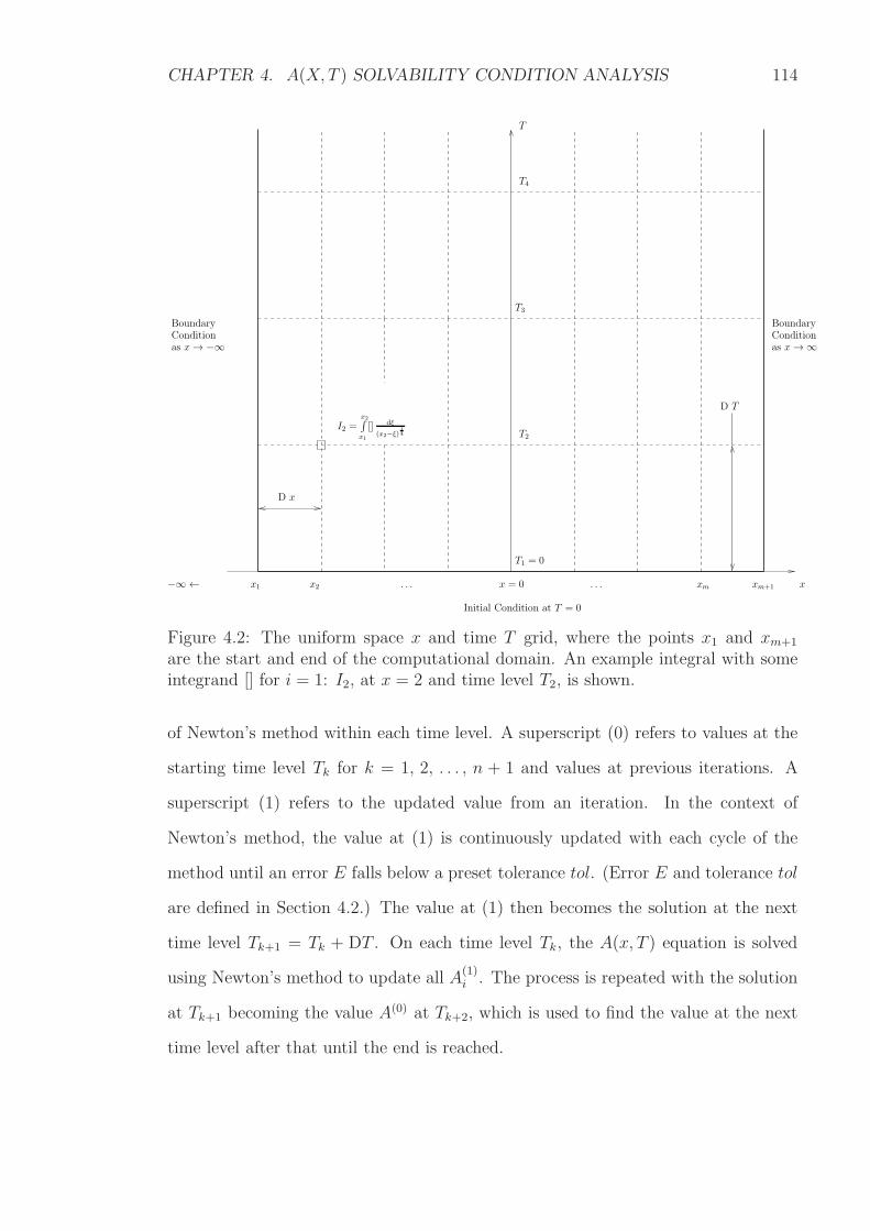
CHAPTER 4. A(X, T ) SOLVABILITY CONDITION ANALYSIS 114
ConditionBoundaryCondition
Boundary
−∞ ← x2 . . . x = 0
Initial Condition at T = 0
. . . xm
T1 = 0
D x
T3
T2
T4
D T
as x→∞
xm+1 xx1
T
as x→ −∞
I2 =x2∫
x1
[] dξ
(x2−ξ)14
Figure 4.2: The uniform space x and time T grid, where the points x1 and xm+1
are the start and end of the computational domain. An example integral with someintegrand [] for i = 1: I2, at x = 2 and time level T2, is shown.
of Newton’s method within each time level. A superscript (0) refers to values at the
starting time level Tk for k = 1, 2, . . . , n + 1 and values at previous iterations. A
superscript (1) refers to the updated value from an iteration. In the context of
Newton’s method, the value at (1) is continuously updated with each cycle of the
method until an error E falls below a preset tolerance tol. (Error E and tolerance tol
are defined in Section 4.2.) The value at (1) then becomes the solution at the next
time level Tk+1 = Tk + DT . On each time level Tk, the A(x, T ) equation is solved
using Newton’s method to update all A(1)i . The process is repeated with the solution
at Tk+1 becoming the value A(0) at Tk+2, which is used to find the value at the next
time level after that until the end is reached.
CHAPTER 4. A(X, T ) SOLVABILITY CONDITION ANALYSIS 115
Centring
“[C]entring at x = xi+ 12, T = T + 1
2DT reflects the implicit elliptic nature of the
problem.”4 The half-subscript i+ 12for space means
xi+ 12=
1
2(xi + xi+1) , i = 1, 2, . . . , m .
Centring in time and space is demonstrated on the left hand side of the (i+1)-th
equation for i = 1, 2, . . . , m, which is discretised as
A2(x, T )− x2 + 2a(T ) =1
4
(
A(1) 2i + A
(1) 2i+1 + A
(0) 2i + A
(0) 2i+1
)
− x2i+ 1
2+(
a(0) + a(1))
(4.7)
The(
a(0) + a(1))
term replaces 2a(T ) because of centring in time, where a(0) is the
value of a at the current time level: a(T ), and a(1) is the value of a at the next
time level: a(T + DT ). Similarly, the first term on the right hand side is so because
A2(x, T ) is centred in both time and space. This left hand side (4.7) will match with
the (i+ 1)-th integral on the right hand side (4.9) later.
Therefore, the A(x, T ) equation (4.1) is reformulated into a system of m nonlinear
equations to solve for Ai and Ai+1 on each time level. On the other hand, there
are only m − 1 unknowns from m + 1 total Ai values minus two known boundary
conditions. On each time level, there are m equations because the method involves
centring. Although the equations are solved for one of the boundary conditions at
each time level Tk, there is the clear condition which states that the solutions should
match with the other boundary condition. The boundary conditions test appears in
the Sections 4.3 and 4.4.
Each (i+1)-th equation uses information at the spatial point x = xi+1 and at all
the points leading up to it from the start of the domain x = x1. Hence, the x term
in the integrand and the upper limit of the (i+1)-th integral becomes x = xi+1. The
4Smith & Elliott (1985)
CHAPTER 4. A(X, T ) SOLVABILITY CONDITION ANALYSIS 116
information at x = xi+1 is the value of Ai+1, known the initial distribution A(0)i+1.
The Integral
The integral on the right hand side of the (i+ 1)-th equation is written as
x∫
−∞
∂A
∂T(ξ, T )
dξ
(x− ξ) 14
=
x1∫
−∞
+
x2∫
x1
+ . . .+
xi+1∫
xi
∂A
∂T(ξ, T )
dξ
(xi+1 − ξ)14
(4.8)
where it is noted that the upper limit of the integral and the x term in the integrand
stop at the specific spatial point x = xi+1. Also, x1 is large and negative with
xi+1 > x1, as in Figure 4.2.
The contribution from the integral with limits from minus infinity to large and
negative x1, calculated at x = xi+1:
x1∫
−∞
∂A
∂T(ξ, T )
dξ
(xi+1 − ξ)14
≃ 0 ,
which can be shown by using the boundary conditions (4.4) and introducing an anti-
clockwise semi-circular contour in the complex plane, as illustrated in Figure 4.3,
such that
x1∫
−∞
=
∮
C
−∫
C1
∂A
∂T(ξ, T )
dξ
(xi+1 − ξ)14
.
By the boundary conditions (4.4), then
∂A
∂T(x, T ) =
da
dT
(
|x|2 + 2a(T ))− 1
2 , |x| → ∞
and from (4.3):
da
dT= 1.332e−T , T ≥ 0 .
CHAPTER 4. A(X, T ) SOLVABILITY CONDITION ANALYSIS 117
Hence, the integral is
1.332e−T ·
x1∫
−∞
=
∮
C
−∫
C1
dξ
(|ξ|2 + 2a(T ))12 (xi+1 − ξ)
14
.
By Cauchy’s residue theorem, as defined in Section 3.3.5, the first integral:
∮
C
dξ
(|ξ|2 + 2a(T ))12 (xi+1 − ξ)
14
= 0
since a(T ) > 0 by (4.3) and there are no singularities of the integrand within the
contour. Additionally, the estimation lemma states:
∣
∣
∣
∣
∣
∣
∫
CR
f(k) dk
∣
∣
∣
∣
∣
∣
≤ l(CR) maxk∈CR
|f(k)|
where
1. the integrand f(k) is a continuous function on the contour CR;
2. the contour CR is a continuous arc;
3. the term l(CR) is the arc length of CR.
Hence, the upper bound of the second integral:
∣
∣
∣
∣
∣
∣
∫
C1
dξ
(|ξ|2 + 2a(T ))12 (xi+1 − ξ)
14
∣
∣
∣
∣
∣
∣
= πR maxθ∈[0,π]
∣
∣
∣
∣
∣
1
(|Reiθ|2 + 2a(T ))12 (xi+1 −Reiθ)
14
∣
∣
∣
∣
∣
→ 0 ,
as R→∞. Therefore, the contribution:5
x1∫
−∞
∂A
∂T(ξ, T )
dξ
(xi+1 − ξ)14
≃ 0
5The contribution does not take into account the next order term of the integrand from theboundary condition (4.4). The contribution is mentioned again in Section 7.4 on further work.
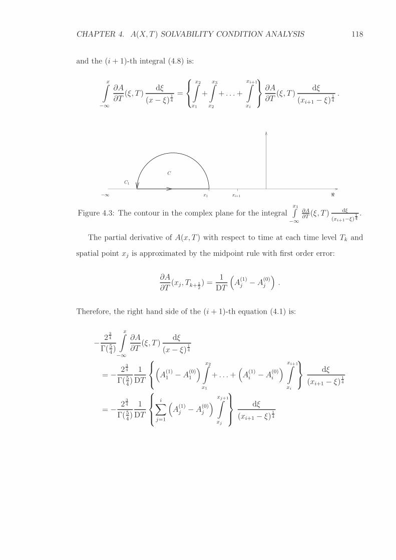
CHAPTER 4. A(X, T ) SOLVABILITY CONDITION ANALYSIS 118
and the (i+ 1)-th integral (4.8) is:
x∫
−∞
∂A
∂T(ξ, T )
dξ
(x− ξ) 14
=
x2∫
x1
+
x3∫
x2
+ . . .+
xi+1∫
xi
∂A
∂T(ξ, T )
dξ
(xi+1 − ξ)14
.
C1
C
ℜ−∞ xi+1x1
Figure 4.3: The contour in the complex plane for the integralx1∫
−∞
∂A∂T
(ξ, T ) dξ
(xi+1−ξ)14.
The partial derivative of A(x, T ) with respect to time at each time level Tk and
spatial point xj is approximated by the midpoint rule with first order error:
∂A
∂T(xj , Tk+ 1
2) =
1
DT
(
A(1)j − A
(0)j
)
.
Therefore, the right hand side of the (i+ 1)-th equation (4.1) is:
− 234
Γ(54)
x∫
−∞
∂A
∂T(ξ, T )
dξ
(x− ξ) 14
= − 234
Γ(54)
1
DT
(
A(1)1 − A
(0)1
)
x2∫
x1
+ . . .+(
A(1)i −A
(0)i
)
xi+1∫
xi
dξ
(xi+1 − ξ)14
= − 234
Γ(54)
1
DT
i∑
j=1
(
A(1)j − A
(0)j
)
xj+1∫
xj
dξ
(xi+1 − ξ)14
CHAPTER 4. A(X, T ) SOLVABILITY CONDITION ANALYSIS 119
which can be solved to give
− 234
Γ(54)
1
DT
i∑
j=1
(
A(1)j − A
(0)j
)
xj+1∫
xj
dξ
(xi+1 − ξ)14
= − 234
Γ(54)
1
DT
i∑
j=1
(
A(1)j −A
(0)j
)
· −43
[
(xi+1 − ξ)34
]xj+1
xj
= − 234
Γ(54)
3
4DT
i∑
j=1
(
A(1)j −A
(0)j
)
·[
(xi+1 − xj)34 − (xi+1 − xj+1)
34
]
= − 234
Γ(54)
3(Dx)34
4DT
i∑
j=1
(
A(1)j −A
(0)j
)
·[
(i+ 1− j) 34 − (i− j) 3
4
]
(4.9)
where Dx and DT are the spatial and time grid steps. This right hand side integral
(4.9) will match with the left hand side term (4.7).
Numerical Treatment
On each time level, the A(x, T ) equation (4.1) becomes a system of m nonlinear
equations of second order accuracy:6
1
4
(
A(1) 2i + A
(1) 2i+1 + A
(0) 2i + A
(0) 2i+1
)
− x2i+ 1
2+(
a(0) + a(1))
= − 234
Γ(54)
3(Dx)34
4DT
i∑
j=1
(
A(1)j −A
(0)j
)
·[
(i+ 1− j) 34 − (i− j) 3
4
]
,
i = 1, 2 . . . , m. (4.10)
The system is regarded as a set of equations of quadratic form for A(1)i which can be
written F(A) = 0 for vectors A = (A1, A2, . . . , Am+1) and 0 = (0, 0, . . . , 0) of m+ 1
components. A component Fi(A) of the system F(A) is
Fi =1
4A
(1) 2i + bA
(1)i + c = 0 (4.11)
6Smith & Elliott (1985)
CHAPTER 4. A(X, T ) SOLVABILITY CONDITION ANALYSIS 120
where
b =2
34
Γ(54)
4(Dx)34
3DT(4.12)
and
c =1
4
(
A(1) 2i+1 + A
(0) 2i + A
(0) 2i+1
)
− x2i+ 1
2+(
a(1) + a(0))
+2
34
Γ(54)
4(Dx)34
3DT·
i−1∑
j=1
(
A(1)j + A
(0)j
) [
(i+ 1− j) 34 − (i− j) 3
4
]
− 234
Γ(54)
4(Dx)34
3DTA
(0)i . (4.13)
The terms bA(1)i and 4(Dx)
34
3DTA
(0)i in c come from the solved integral summation (4.9)
when j = i. For i = 1:
F1
(
A(1))
=1
4A
(1) 21 +
234
Γ(54)
4(Dx)34
3DTA
(1)1
+
1
4
(
A(1) 22 + A
(0) 21 + A
(0) 22
)
−(
x1 + x22
)2
+(
a(1) + a(0))
− 234
Γ(54)
4(Dx)34
3DTA
(0)1
= 0 ; (4.14)
for i = 2:
F2
(
A(1))
=1
4A
(1) 22 +
234
Γ(54)
4(Dx)34
3DTA
(1)2
+
1
4
(
A(1) 23 + A
(0) 22 + A
(0) 23
)
−(
x2 + x32
)2
+(
a(1) + a(0))
+2
34
Γ(54)
4(Dx)34
3DT
(
A(1)1 + A
(0)1
) [
234 − 1
34
]
− 234
Γ(54)
4(Dx)34
3DTA
(0)2
= 0 (4.15)
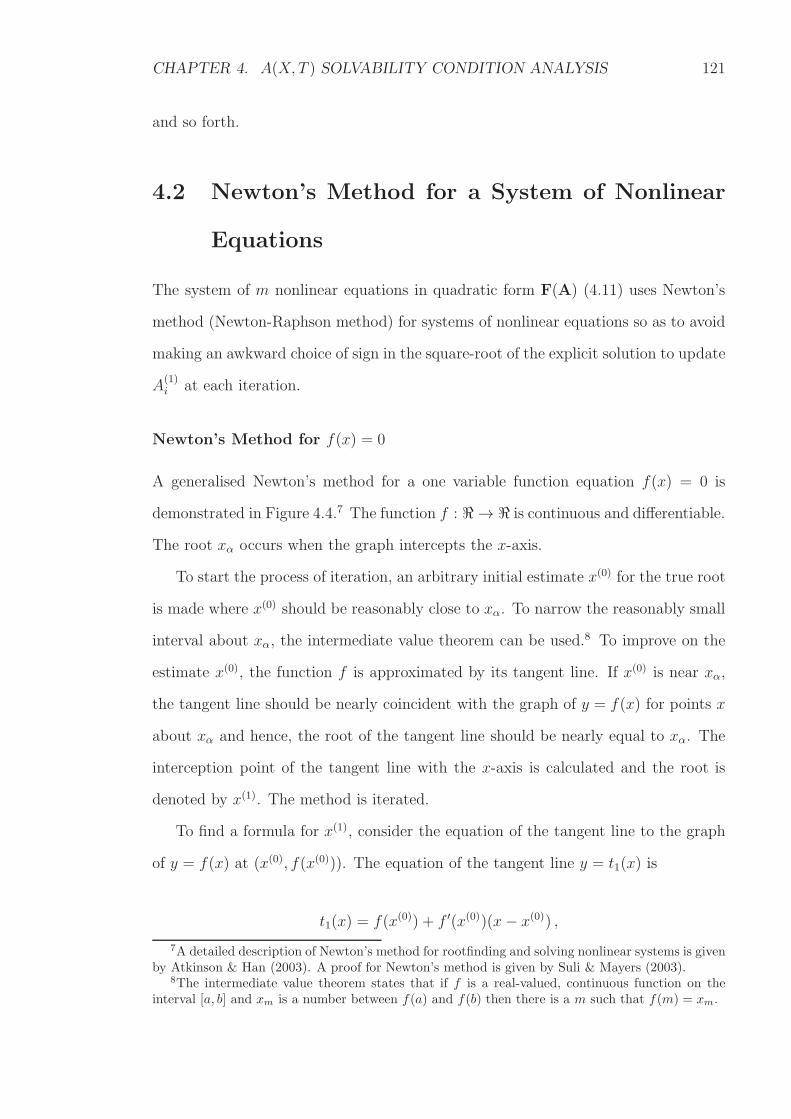
CHAPTER 4. A(X, T ) SOLVABILITY CONDITION ANALYSIS 121
and so forth.
4.2 Newton’s Method for a System of Nonlinear
Equations
The system of m nonlinear equations in quadratic form F(A) (4.11) uses Newton’s
method (Newton-Raphson method) for systems of nonlinear equations so as to avoid
making an awkward choice of sign in the square-root of the explicit solution to update
A(1)i at each iteration.
Newton’s Method for f(x) = 0
A generalised Newton’s method for a one variable function equation f(x) = 0 is
demonstrated in Figure 4.4.7 The function f : ℜ → ℜ is continuous and differentiable.
The root xα occurs when the graph intercepts the x-axis.
To start the process of iteration, an arbitrary initial estimate x(0) for the true root
is made where x(0) should be reasonably close to xα. To narrow the reasonably small
interval about xα, the intermediate value theorem can be used.8 To improve on the
estimate x(0), the function f is approximated by its tangent line. If x(0) is near xα,
the tangent line should be nearly coincident with the graph of y = f(x) for points x
about xα and hence, the root of the tangent line should be nearly equal to xα. The
interception point of the tangent line with the x-axis is calculated and the root is
denoted by x(1). The method is iterated.
To find a formula for x(1), consider the equation of the tangent line to the graph
of y = f(x) at (x(0), f(x(0))). The equation of the tangent line y = t1(x) is
t1(x) = f(x(0)) + f ′(x(0))(x− x(0)) ,7A detailed description of Newton’s method for rootfinding and solving nonlinear systems is given
by Atkinson & Han (2003). A proof for Newton’s method is given by Suli & Mayers (2003).8The intermediate value theorem states that if f is a real-valued, continuous function on the
interval [a, b] and xm is a number between f(a) and f(b) then there is a m such that f(m) = xm.
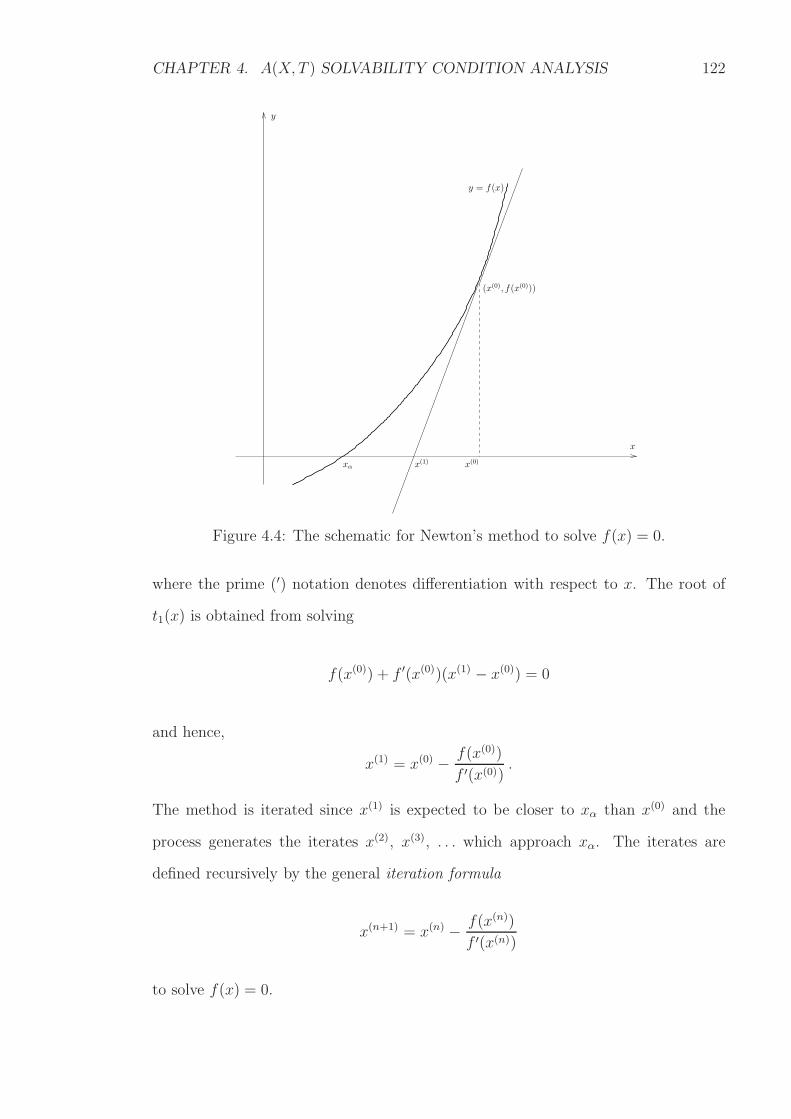
CHAPTER 4. A(X, T ) SOLVABILITY CONDITION ANALYSIS 122
y
x
x(0)xα x(1)
(x(0), f(x(0)))
y = f(x)
Figure 4.4: The schematic for Newton’s method to solve f(x) = 0.
where the prime (′) notation denotes differentiation with respect to x. The root of
t1(x) is obtained from solving
f(x(0)) + f ′(x(0))(x(1) − x(0)) = 0
and hence,
x(1) = x(0) − f(x(0))
f ′(x(0)).
The method is iterated since x(1) is expected to be closer to xα than x(0) and the
process generates the iterates x(2), x(3), . . . which approach xα. The iterates are
defined recursively by the general iteration formula
x(n+1) = x(n) − f(x(n))
f ′(x(n))
to solve f(x) = 0.
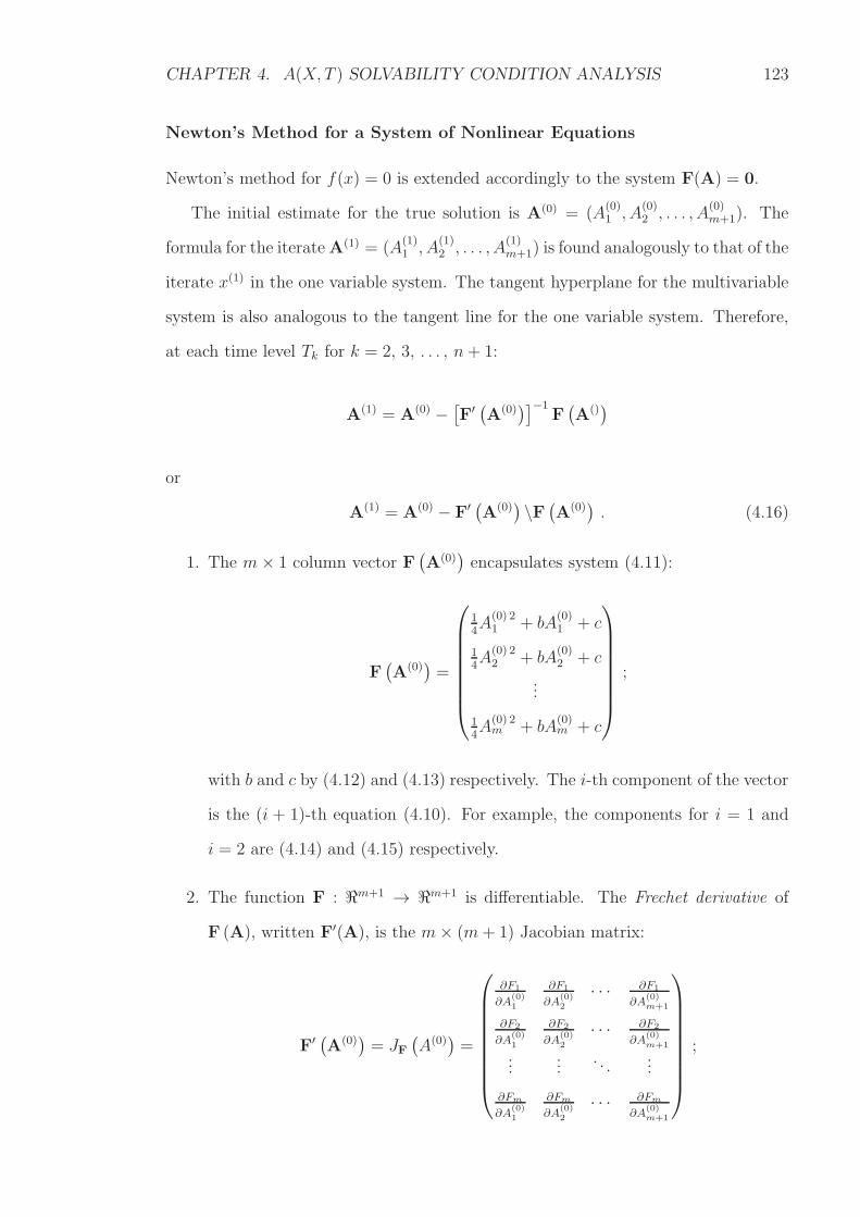
CHAPTER 4. A(X, T ) SOLVABILITY CONDITION ANALYSIS 123
Newton’s Method for a System of Nonlinear Equations
Newton’s method for f(x) = 0 is extended accordingly to the system F(A) = 0.
The initial estimate for the true solution is A(0) = (A(0)1 , A
(0)2 , . . . , A
(0)m+1). The
formula for the iterateA(1) = (A(1)1 , A
(1)2 , . . . , A
(1)m+1) is found analogously to that of the
iterate x(1) in the one variable system. The tangent hyperplane for the multivariable
system is also analogous to the tangent line for the one variable system. Therefore,
at each time level Tk for k = 2, 3, . . . , n+ 1:
A(1) = A(0) −[
F′(
A(0))]−1
F(
A())
or
A(1) = A(0) − F′(
A(0))
\F(
A(0))
. (4.16)
1. The m× 1 column vector F(
A(0))
encapsulates system (4.11):
F(
A(0))
=
14A
(0) 21 + bA
(0)1 + c
14A
(0) 22 + bA
(0)2 + c
...
14A
(0) 2m + bA
(0)m + c
;
with b and c by (4.12) and (4.13) respectively. The i-th component of the vector
is the (i + 1)-th equation (4.10). For example, the components for i = 1 and
i = 2 are (4.14) and (4.15) respectively.
2. The function F : ℜm+1 → ℜm+1 is differentiable. The Frechet derivative of
F (A), written F′(A), is the m× (m+ 1) Jacobian matrix:
F′(
A(0))
= JF(
A(0))
=
∂F1
∂A(0)1
∂F1
∂A(0)2
· · · ∂F1
∂A(0)m+1
∂F2
∂A(0)1
∂F2
∂A(0)2
· · · ∂F2
∂A(0)m+1
......
. . ....
∂Fm
∂A(0)1
∂Fm
∂A(0)2
· · · ∂Fm
∂A(0)m+1
;
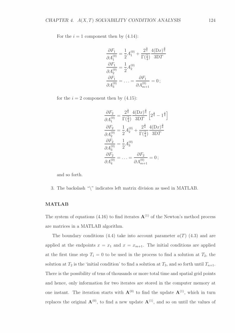
CHAPTER 4. A(X, T ) SOLVABILITY CONDITION ANALYSIS 124
For the i = 1 component then by (4.14):
∂F1
∂A(0)1
=1
2A
(0)1 +
234
Γ(54)
4(Dx)34
3DT
∂F1
∂A(0)2
=1
2A
(0)2
∂F1
∂A(0)3
= . . . =∂F1
∂A(0)m+1
= 0 ;
for the i = 2 component then by (4.15):
∂F2
∂A(0)1
=2
34
Γ(54)
4(Dx)34
3DT
[
234 − 1
34
]
∂F2
∂A(0)2
=1
2A
(0)2 +
234
Γ(54)
4(Dx)34
3DT
∂F2
∂A(0)3
=1
2A
(0)3
∂F2
∂A(0)4
= . . . =∂F2
∂A(0)m+1
= 0 ;
and so forth.
3. The backslash “\” indicates left matrix division as used in MATLAB.
MATLAB
The system of equations (4.16) to find iterates A(1) of the Newton’s method process
are matrices in a MATLAB algorithm.
The boundary conditions (4.4) take into account parameter a(T ) (4.3) and are
applied at the endpoints x = x1 and x = xm+1. The initial conditions are applied
at the first time step T1 = 0 to be used in the process to find a solution at T2, the
solution at T2 is the ‘initial condition’ to find a solution at T3, and so forth until Tn+1.
There is the possibility of tens of thousands or more total time and spatial grid points
and hence, only information for two iterates are stored in the computer memory at
one instant. The iteration starts with A(0) to find the update A(1), which in turn
replaces the original A(0), to find a new update A(1), and so on until the values of
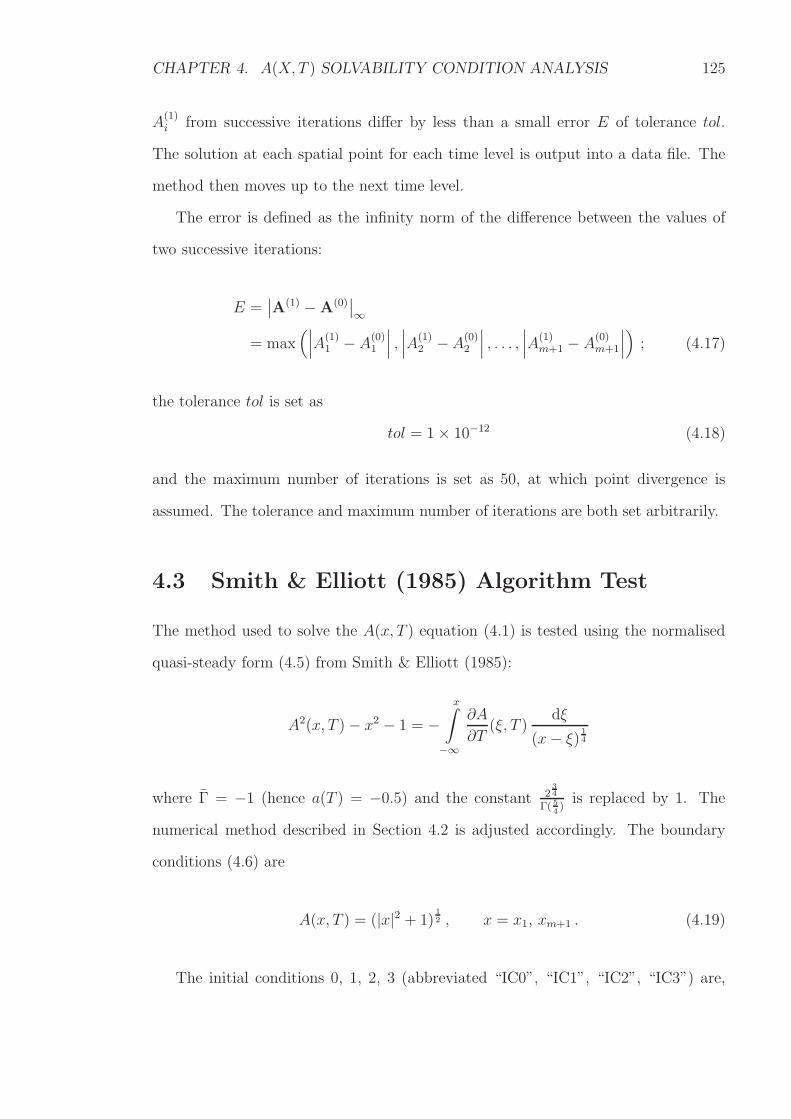
CHAPTER 4. A(X, T ) SOLVABILITY CONDITION ANALYSIS 125
A(1)i from successive iterations differ by less than a small error E of tolerance tol.
The solution at each spatial point for each time level is output into a data file. The
method then moves up to the next time level.
The error is defined as the infinity norm of the difference between the values of
two successive iterations:
E =∣
∣A(1) −A(0)∣
∣
∞
= max(∣
∣
∣A
(1)1 − A
(0)1
∣
∣
∣,∣
∣
∣A
(1)2 −A
(0)2
∣
∣
∣, . . . ,
∣
∣
∣A
(1)m+1 − A
(0)m+1
∣
∣
∣
)
; (4.17)
the tolerance tol is set as
tol = 1× 10⁻¹² (4.18)
and the maximum number of iterations is set as 50, at which point divergence is
assumed. The tolerance and maximum number of iterations are both set arbitrarily.
4.3 Smith & Elliott (1985) Algorithm Test
The method used to solve the A(x, T ) equation (4.1) is tested using the normalised
quasi-steady form (4.5) from Smith & Elliott (1985):
A2(x, T )− x2 − 1 = −x∫
−∞
∂A
∂T(ξ, T )
dξ
(x− ξ) 14
where Γ = −1 (hence a(T ) = −0.5) and the constant 234
Γ( 54)is replaced by 1. The
numerical method described in Section 4.2 is adjusted accordingly. The boundary
conditions (4.6) are
A(x, T ) = (|x|2 + 1)12 , x = x1, xm+1 . (4.19)
The initial conditions 0, 1, 2, 3 (abbreviated “IC0”, “IC1”, “IC2”, “IC3”) are,
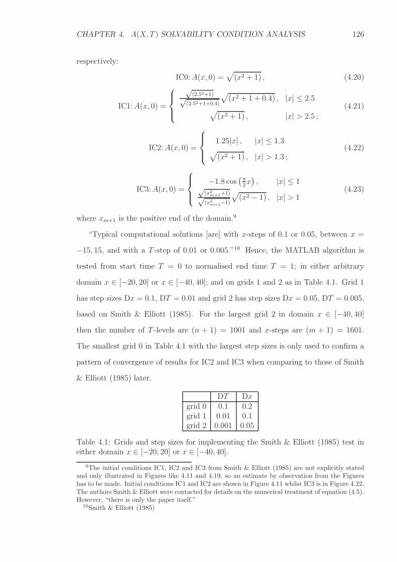
CHAPTER 4. A(X, T ) SOLVABILITY CONDITION ANALYSIS 126
respectively:
IC0:A(x, 0) =√
(x2 + 1) , (4.20)
IC1:A(x, 0) =
√(2.52+1)√
(2.52+1+0.4)
√
(x2 + 1 + 0.4) , |x| ≤ 2.5
√
(x2 + 1) , |x| > 2.5 ;
(4.21)
IC2:A(x, 0) =
1.25|x| , |x| ≤ 1.3√
(x2 + 1) , |x| > 1.3 ;(4.22)
IC3:A(x, 0) =
−1.8 cos(
π2x)
, |x| ≤ 1√(x2
m+1+1)√(x2
m+1−1)
√
(x2 − 1) , |x| > 1(4.23)
where xm+1 is the positive end of the domain.9
“Typical computational solutions [are] with x-steps of 0.1 or 0.05, between x =
−15, 15, and with a T -step of 0.01 or 0.005.”10 Hence, the MATLAB algorithm is
tested from start time T = 0 to normalised end time T = 1; in either arbitrary
domain x ∈ [−20, 20] or x ∈ [−40, 40]; and on grids 1 and 2 as in Table 4.1. Grid 1
has step sizes Dx = 0.1, DT = 0.01 and grid 2 has step sizes Dx = 0.05, DT = 0.005,
based on Smith & Elliott (1985). For the largest grid 2 in domain x ∈ [−40, 40]
then the number of T -levels are (n + 1) = 1001 and x-steps are (m + 1) = 1601.
The smallest grid 0 in Table 4.1 with the largest step sizes is only used to confirm a
pattern of convergence of results for IC2 and IC3 when comparing to those of Smith
& Elliott (1985) later.
DT Dxgrid 0 0.1 0.2grid 1 0.01 0.1grid 2 0.001 0.05
Table 4.1: Grids and step sizes for implementing the Smith & Elliott (1985) test ineither domain x ∈ [−20, 20] or x ∈ [−40, 40].
9The initial conditions IC1, IC2 and IC3 from Smith & Elliott (1985) are not explicitly statedand only illustrated in Figures like 4.11 and 4.19, so an estimate by observation from the Figureshas to be made. Initial conditions IC1 and IC2 are shown in Figure 4.11 whilst IC3 is in Figure 4.22.The authors Smith & Elliott were contacted for details on the numerical treatment of equation (4.5).However, “there is only the paper itself.”
10Smith & Elliott (1985)
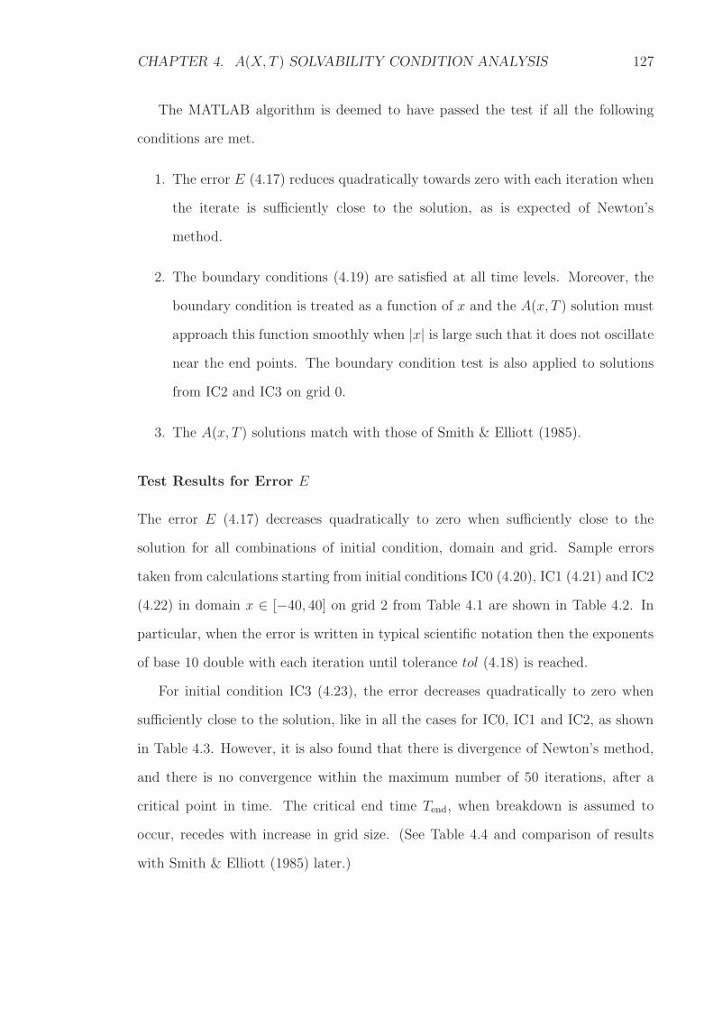
CHAPTER 4. A(X, T ) SOLVABILITY CONDITION ANALYSIS 127
The MATLAB algorithm is deemed to have passed the test if all the following
conditions are met.
1. The error E (4.17) reduces quadratically towards zero with each iteration when
the iterate is sufficiently close to the solution, as is expected of Newton’s
method.
2. The boundary conditions (4.19) are satisfied at all time levels. Moreover, the
boundary condition is treated as a function of x and the A(x, T ) solution must
approach this function smoothly when |x| is large such that it does not oscillate
near the end points. The boundary condition test is also applied to solutions
from IC2 and IC3 on grid 0.
3. The A(x, T ) solutions match with those of Smith & Elliott (1985).
Test Results for Error E
The error E (4.17) decreases quadratically to zero when sufficiently close to the
solution for all combinations of initial condition, domain and grid. Sample errors
taken from calculations starting from initial conditions IC0 (4.20), IC1 (4.21) and IC2
(4.22) in domain x ∈ [−40, 40] on grid 2 from Table 4.1 are shown in Table 4.2. In
particular, when the error is written in typical scientific notation then the exponents
of base 10 double with each iteration until tolerance tol (4.18) is reached.
For initial condition IC3 (4.23), the error decreases quadratically to zero when
sufficiently close to the solution, like in all the cases for IC0, IC1 and IC2, as shown
in Table 4.3. However, it is also found that there is divergence of Newton’s method,
and there is no convergence within the maximum number of 50 iterations, after a
critical point in time. The critical end time Tend, when breakdown is assumed to
occur, recedes with increase in grid size. (See Table 4.4 and comparison of results
with Smith & Elliott (1985) later.)
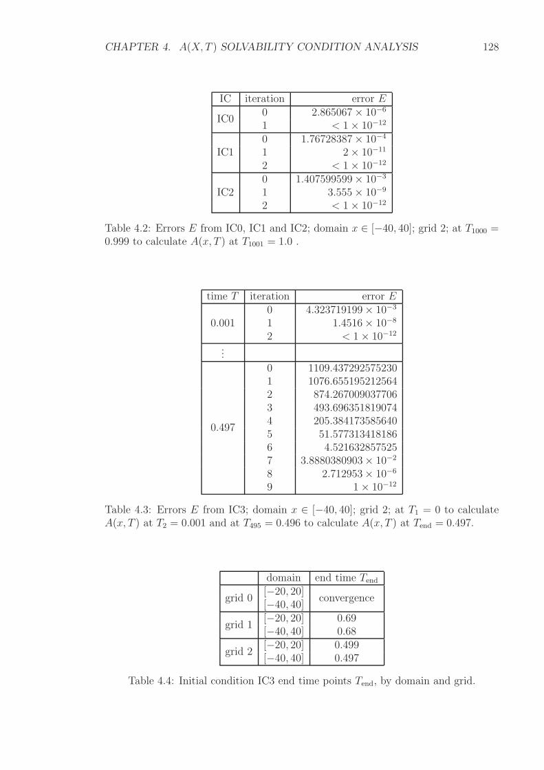
CHAPTER 4. A(X, T ) SOLVABILITY CONDITION ANALYSIS 128
IC iteration error E
IC00 2.865067× 10⁻⁶
1 < 1× 10⁻¹²
IC10 1.76728387× 10⁻⁴
1 2× 10⁻¹¹
2 < 1× 10⁻¹²
IC20 1.407599599× 10⁻³
1 3.555× 10⁻⁹
2 < 1× 10⁻¹²
Table 4.2: Errors E from IC0, IC1 and IC2; domain x ∈ [−40, 40]; grid 2; at T1000 =0.999 to calculate A(x, T ) at T1001 = 1.0 .
time T iteration error E
0.0010 4.323719199× 10⁻³
1 1.4516× 10⁻⁸
2 < 1× 10⁻¹²
...
0.497
0 1109.4372925752301 1076.6551952125642 874.2670090377063 493.6963518190744 205.3841735856405 51.5773134181866 4.5216328575257 3.8880380903× 10⁻²
8 2.712953× 10⁻⁶
9 1× 10⁻¹²
Table 4.3: Errors E from IC3; domain x ∈ [−40, 40]; grid 2; at T1 = 0 to calculateA(x, T ) at T2 = 0.001 and at T495 = 0.496 to calculate A(x, T ) at Tend = 0.497.
domain end time Tend
grid 0[−20, 20]
convergence[−40, 40]
grid 1[−20, 20] 0.69[−40, 40] 0.68
grid 2[−20, 20] 0.499[−40, 40] 0.497
Table 4.4: Initial condition IC3 end time points Tend, by domain and grid.
CHAPTER 4. A(X, T ) SOLVABILITY CONDITION ANALYSIS 129
Test Results for Boundary Conditions
For all possible combinations of initial condition, domain and grid, the solutions
matched the boundary conditions (4.19) for all time. The boundary condition func-
tion and the solutions are shown at sample time points as coinciding lines in the
regions outside a small neighbourhood of the origin x = 0 in Figures 4.5 to 4.8.
Indeed for the steady state initial condition IC0 (4.20), which coincides with the
boundary condition, there is no deviation from the start such that the solutions
remain the same for all time. (See Figure 4.5.)
For initial condition IC3 (4.23), there is no convergence of Newton’s method after
the end time Tend. (See test results for error E and end times in Table 4.4.) However,
the boundary conditions are still satisfied up to the end time.
Note that solutions near the origin in Figures 4.5 to 4.8, which can appear like
oscillations, can be ignored here since the Figures intend to show that solutions satisfy
the boundary conditions at the ends of the computational domain.
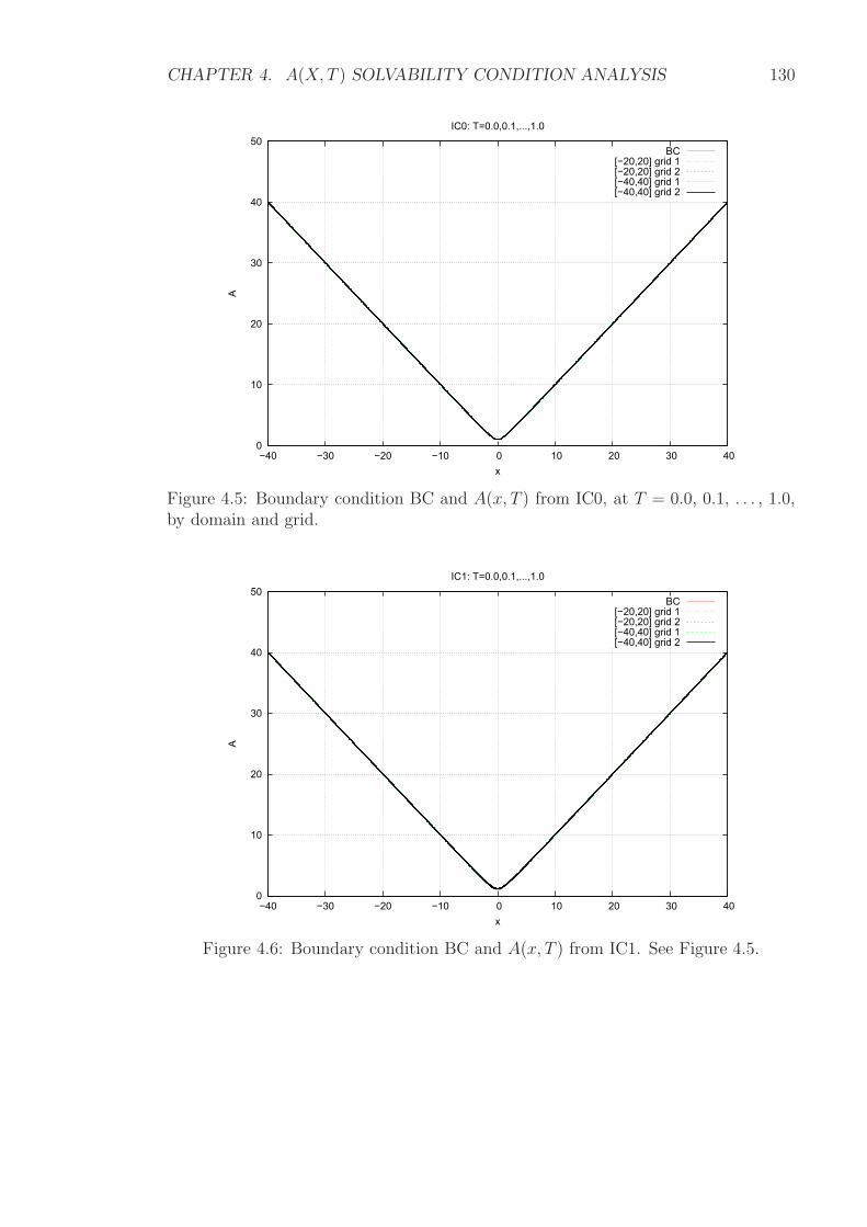
CHAPTER 4. A(X, T ) SOLVABILITY CONDITION ANALYSIS 130
0
10
20
30
40
50
−40 −30 −20 −10 0 10 20 30 40
A
x
IC0: T=0.0,0.1,...,1.0
BC[−20,20] grid 1[−20,20] grid 2[−40,40] grid 1[−40,40] grid 2
Figure 4.5: Boundary condition BC and A(x, T ) from IC0, at T = 0.0, 0.1, . . . , 1.0,by domain and grid.
0
10
20
30
40
50
−40 −30 −20 −10 0 10 20 30 40
A
x
IC1: T=0.0,0.1,...,1.0
BC[−20,20] grid 1[−20,20] grid 2[−40,40] grid 1[−40,40] grid 2
Figure 4.6: Boundary condition BC and A(x, T ) from IC1. See Figure 4.5.
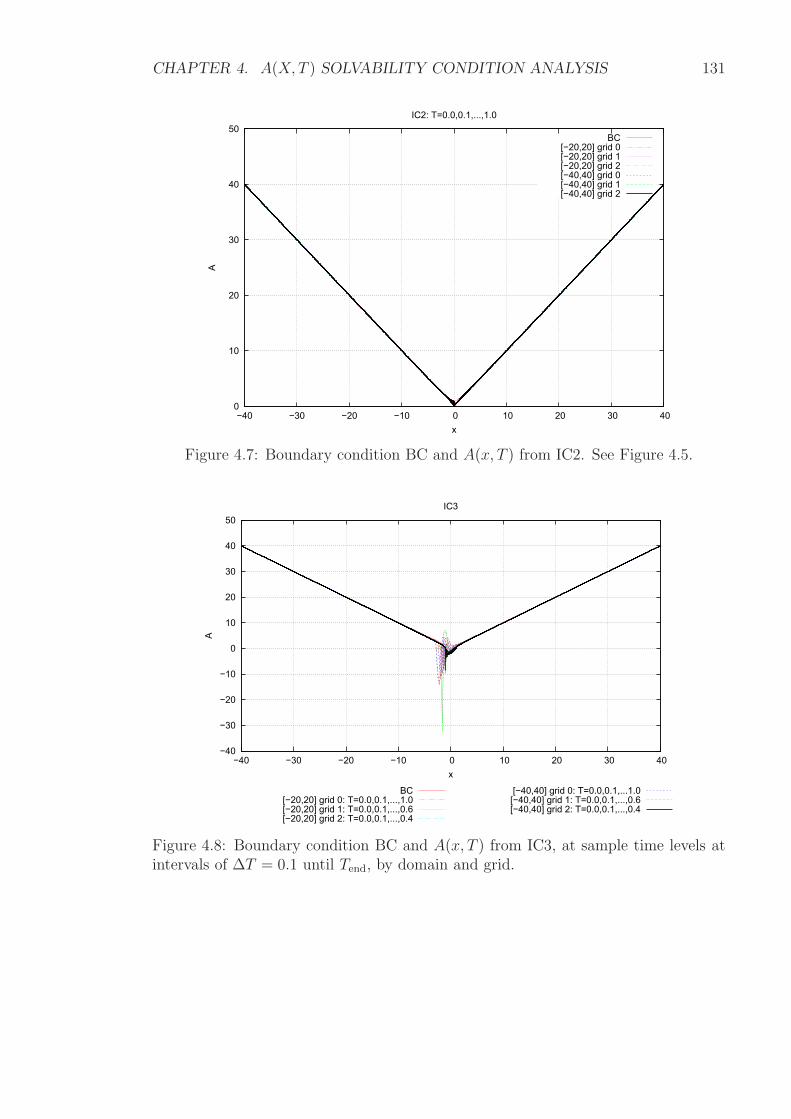
CHAPTER 4. A(X, T ) SOLVABILITY CONDITION ANALYSIS 131
0
10
20
30
40
50
−40 −30 −20 −10 0 10 20 30 40
A
x
IC2: T=0.0,0.1,...,1.0
BC[−20,20] grid 0[−20,20] grid 1[−20,20] grid 2[−40,40] grid 0[−40,40] grid 1[−40,40] grid 2
Figure 4.7: Boundary condition BC and A(x, T ) from IC2. See Figure 4.5.
−40
−30
−20
−10
0
10
20
30
40
50
−40 −30 −20 −10 0 10 20 30 40
A
x
IC3
BC[−20,20] grid 0: T=0.0,0.1,...,1.0[−20,20] grid 1: T=0.0,0.1,...,0.6[−20,20] grid 2: T=0.0,0.1,...,0.4
[−40,40] grid 0: T=0.0,0.1,...1.0[−40,40] grid 1: T=0.0,0.1,...,0.6[−40,40] grid 2: T=0.0,0.1,...,0.4
Figure 4.8: Boundary condition BC and A(x, T ) from IC3, at sample time levels atintervals of ∆T = 0.1 until Tend, by domain and grid.
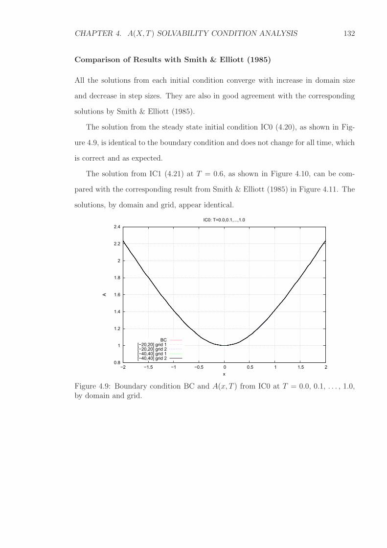
CHAPTER 4. A(X, T ) SOLVABILITY CONDITION ANALYSIS 132
Comparison of Results with Smith & Elliott (1985)
All the solutions from each initial condition converge with increase in domain size
and decrease in step sizes. They are also in good agreement with the corresponding
solutions by Smith & Elliott (1985).
The solution from the steady state initial condition IC0 (4.20), as shown in Fig-
ure 4.9, is identical to the boundary condition and does not change for all time, which
is correct and as expected.
The solution from IC1 (4.21) at T = 0.6, as shown in Figure 4.10, can be com-
pared with the corresponding result from Smith & Elliott (1985) in Figure 4.11. The
solutions, by domain and grid, appear identical.
0.8
1
1.2
1.4
1.6
1.8
2
2.2
2.4
−2 −1.5 −1 −0.5 0 0.5 1 1.5 2
A
x
IC0: T=0.0,0.1,...,1.0
BC[−20,20] grid 1[−20,20] grid 2[−40,40] grid 1[−40,40] grid 2
Figure 4.9: Boundary condition BC and A(x, T ) from IC0 at T = 0.0, 0.1, . . . , 1.0,by domain and grid.
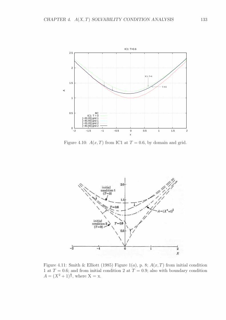
CHAPTER 4. A(X, T ) SOLVABILITY CONDITION ANALYSIS 133
0
0.5
1
1.5
2
2.5
−2 −1.5 −1 −0.5 0 0.5 1 1.5 2
A
x
IC1: T=0.6
BCIC1: T = 0
[−20,20] grid 1[−40,40] grid 1[−20,20] grid 2[−40,40] grid 2
IC1: T=0
T=0.6
Figure 4.10: A(x, T ) from IC1 at T = 0.6, by domain and grid.
Figure 4.11: Smith & Elliott (1985) Figure 1(a), p. 8; A(x, T ) from initial condition1 at T = 0.6; and from initial condition 2 at T = 0.9; also with boundary conditionA = (X2 + 1)
12 , where X = x.
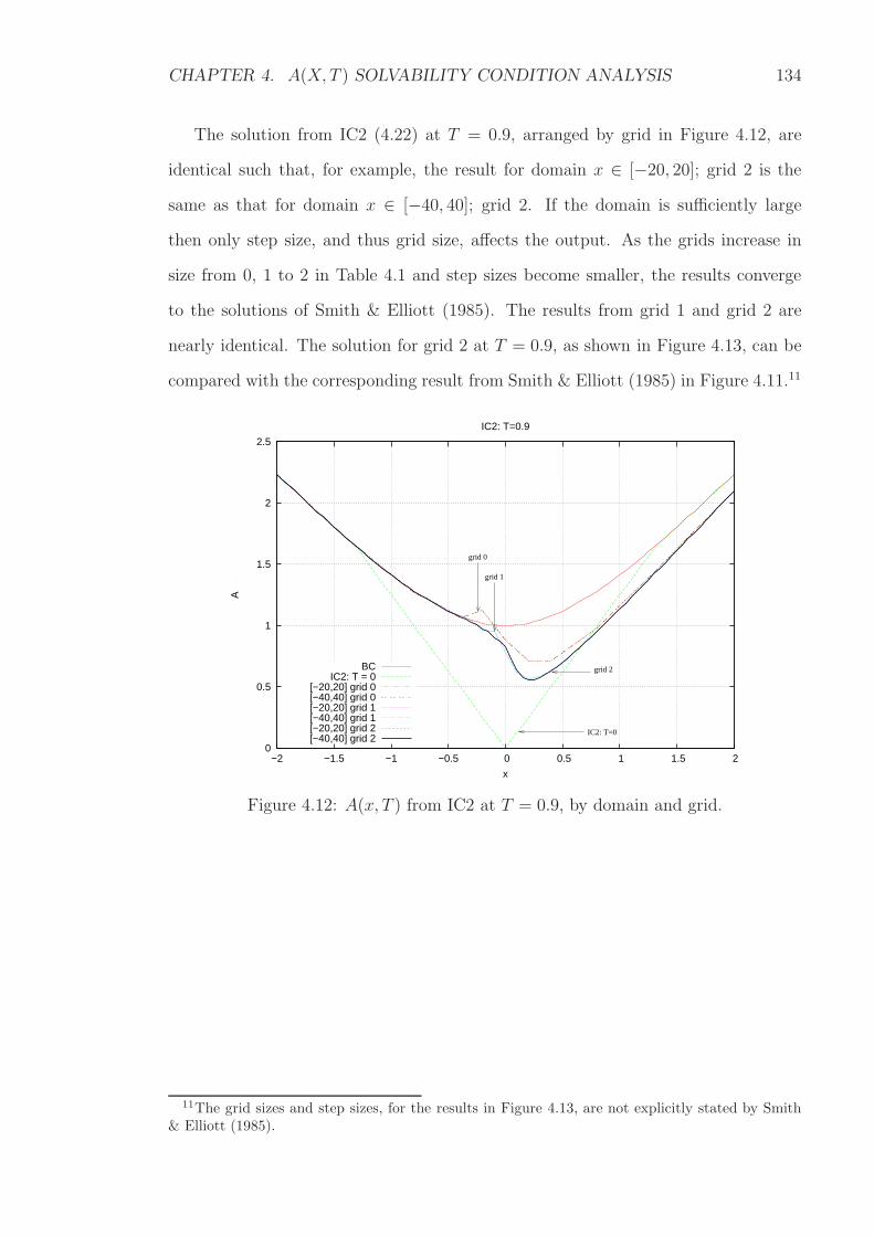
CHAPTER 4. A(X, T ) SOLVABILITY CONDITION ANALYSIS 134
The solution from IC2 (4.22) at T = 0.9, arranged by grid in Figure 4.12, are
identical such that, for example, the result for domain x ∈ [−20, 20]; grid 2 is the
same as that for domain x ∈ [−40, 40]; grid 2. If the domain is sufficiently large
then only step size, and thus grid size, affects the output. As the grids increase in
size from 0, 1 to 2 in Table 4.1 and step sizes become smaller, the results converge
to the solutions of Smith & Elliott (1985). The results from grid 1 and grid 2 are
nearly identical. The solution for grid 2 at T = 0.9, as shown in Figure 4.13, can be
compared with the corresponding result from Smith & Elliott (1985) in Figure 4.11.11
0
0.5
1
1.5
2
2.5
−2 −1.5 −1 −0.5 0 0.5 1 1.5 2
A
x
IC2: T=0.9
BCIC2: T = 0
[−20,20] grid 0[−40,40] grid 0[−20,20] grid 1[−40,40] grid 1[−20,20] grid 2[−40,40] grid 2
grid 0
grid 1
IC2: T=0
grid 2
Figure 4.12: A(x, T ) from IC2 at T = 0.9, by domain and grid.
11The grid sizes and step sizes, for the results in Figure 4.13, are not explicitly stated by Smith& Elliott (1985).
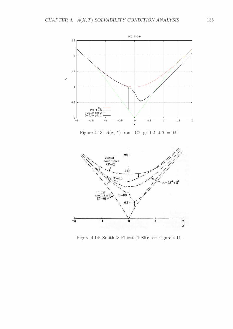
CHAPTER 4. A(X, T ) SOLVABILITY CONDITION ANALYSIS 135
0
0.5
1
1.5
2
2.5
−2 −1.5 −1 −0.5 0 0.5 1 1.5 2
A
x
IC2: T=0.9
BCIC2: T = 0
[−20,20] grid 2[−40,40] grid 2
Figure 4.13: A(x, T ) from IC2, grid 2 at T = 0.9.
Figure 4.14: Smith & Elliott (1985); see Figure 4.11.
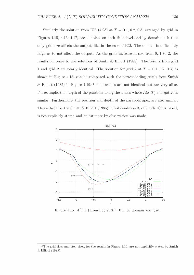
CHAPTER 4. A(X, T ) SOLVABILITY CONDITION ANALYSIS 136
Similarly the solution from IC3 (4.23) at T = 0.1, 0.2, 0.3, arranged by grid in
Figures 4.15, 4.16, 4.17, are identical on each time level and by domain such that
only grid size affects the output, like in the case of IC2. The domain is sufficiently
large as to not affect the output. As the grids increase in size from 0, 1 to 2, the
results converge to the solutions of Smith & Elliott (1985). The results from grid
1 and grid 2 are nearly identical. The solution for grid 2 at T = 0.1, 0.2, 0.3, as
shown in Figure 4.18, can be compared with the corresponding result from Smith
& Elliott (1985) in Figure 4.19.12 The results are not identical but are very alike.
For example, the length of the parabola along the x-axis where A(x, T ) is negative is
similar. Furthermore, the position and depth of the parabola apex are also similar.
This is because the Smith & Elliott (1985) initial condition 3, of which IC3 is based,
is not explicitly stated and an estimate by observation was made.
−3
−2
−1
0
1
2
3
−1.5 −1 −0.5 0 0.5 1 1.5
A
x
IC3: T=0.1
BCIC3: T = 0
[−20,20] grid 0[−40,40] grid 0[−20,20] grid 1[−40,40] grid 1[−20,20] grid 2[−40,40] grid 2
grid 0
grid 1
IC3: T=0grid 2
Figure 4.15: A(x, T ) from IC3 at T = 0.1, by domain and grid.
12The grid sizes and step sizes, for the results in Figure 4.19, are not explicitly stated by Smith& Elliott (1985).
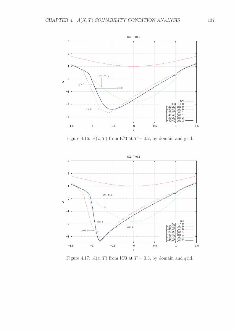
CHAPTER 4. A(X, T ) SOLVABILITY CONDITION ANALYSIS 137
−3
−2
−1
0
1
2
3
−1.5 −1 −0.5 0 0.5 1 1.5
A
x
IC3: T=0.2
BCIC3: T = 0
[−20,20] grid 0[−40,40] grid 0[−20,20] grid 1[−40,40] grid 1[−20,20] grid 2[−40,40] grid 2
grid 0
grid 1
grid 2
IC3: T=0
Figure 4.16: A(x, T ) from IC3 at T = 0.2, by domain and grid.
−3
−2
−1
0
1
2
3
−1.5 −1 −0.5 0 0.5 1 1.5
A
x
IC3: T=0.3
BCIC3: T = 0
[−20,20] grid 0[−40,40] grid 0[−20,20] grid 1[−40,40] grid 1[−20,20] grid 2[−40,40] grid 2
grid 0
grid 1
grid 2
IC3: T=0
Figure 4.17: A(x, T ) from IC3 at T = 0.3, by domain and grid.
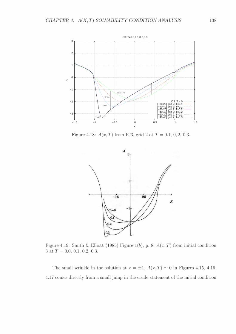
CHAPTER 4. A(X, T ) SOLVABILITY CONDITION ANALYSIS 138
−3
−2
−1
0
1
2
3
−1.5 −1 −0.5 0 0.5 1 1.5
A
x
IC3: T=0.0,0.1,0.2,0.3
IC3: T = 0[−20,20] grid 2: T=0.1[−40,40] grid 2: T=0.1[−20,20] grid 2: T=0.2[−40,40] grid 2: T=0.2[−20,20] grid 2: T=0.3[−40,40] grid 2: T=0.3
T=0.1
T=0.2
T=0.3
IC3: T=0
Figure 4.18: A(x, T ) from IC3, grid 2 at T = 0.1, 0, 2, 0.3.
Figure 4.19: Smith & Elliott (1985) Figure 1(b), p. 8; A(x, T ) from initial condition3 at T = 0.0, 0.1, 0.2, 0.3.
The small wrinkle in the solution at x = ±1, A(x, T ) ≃ 0 in Figures 4.15, 4.16,
4.17 comes directly from a small jump in the crude statement of the initial condition
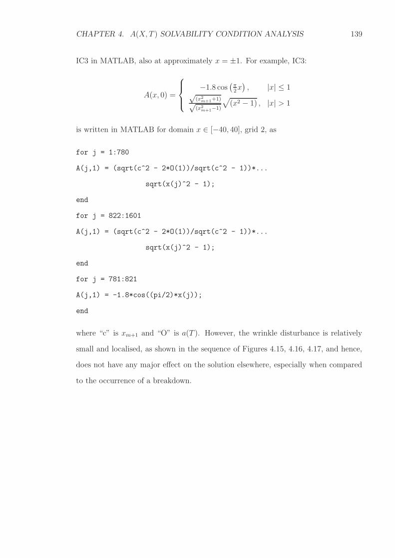
CHAPTER 4. A(X, T ) SOLVABILITY CONDITION ANALYSIS 139
IC3 in MATLAB, also at approximately x = ±1. For example, IC3:
A(x, 0) =
−1.8 cos(
π2x)
, |x| ≤ 1√(x2
m+1+1)√(x2
m+1−1)
√
(x2 − 1) , |x| > 1
is written in MATLAB for domain x ∈ [−40, 40], grid 2, as
for j = 1:780
A(j,1) = (sqrt(c^2 - 2*O(1))/sqrt(c^2 - 1))*...
sqrt(x(j)^2 - 1);
end
for j = 822:1601
A(j,1) = (sqrt(c^2 - 2*O(1))/sqrt(c^2 - 1))*...
sqrt(x(j)^2 - 1);
end
for j = 781:821
A(j,1) = -1.8*cos((pi/2)*x(j));
end
where “c” is xm+1 and “O” is a(T ). However, the wrinkle disturbance is relatively
small and localised, as shown in the sequence of Figures 4.15, 4.16, 4.17, and hence,
does not have any major effect on the solution elsewhere, especially when compared
to the occurrence of a breakdown.
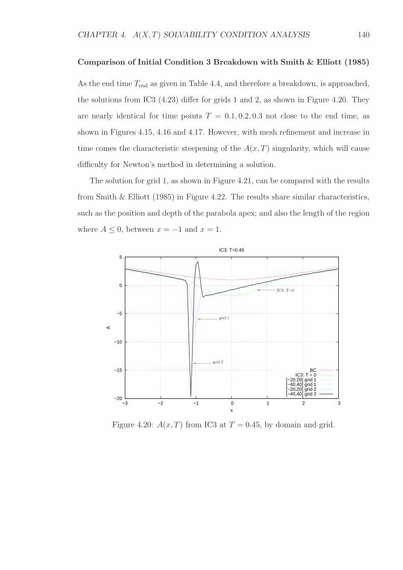
CHAPTER 4. A(X, T ) SOLVABILITY CONDITION ANALYSIS 140
Comparison of Initial Condition 3 Breakdown with Smith & Elliott (1985)
As the end time Tend as given in Table 4.4, and therefore a breakdown, is approached,
the solutions from IC3 (4.23) differ for grids 1 and 2, as shown in Figure 4.20. They
are nearly identical for time points T = 0.1, 0.2, 0.3 not close to the end time, as
shown in Figures 4.15, 4.16 and 4.17. However, with mesh refinement and increase in
time comes the characteristic steepening of the A(x, T ) singularity, which will cause
difficulty for Newton’s method in determining a solution.
The solution for grid 1, as shown in Figure 4.21, can be compared with the results
from Smith & Elliott (1985) in Figure 4.22. The results share similar characteristics,
such as the position and depth of the parabola apex; and also the length of the region
where A ≤ 0, between x = −1 and x = 1.
−20
−15
−10
−5
0
5
−3 −2 −1 0 1 2 3
A
x
IC3: T=0.45
BCIC3: T = 0
[−20,20] grid 1[−40,40] grid 1[−20,20] grid 2[−40,40] grid 2
grid 1
grid 2
IC3: T=0
Figure 4.20: A(x, T ) from IC3 at T = 0.45, by domain and grid.
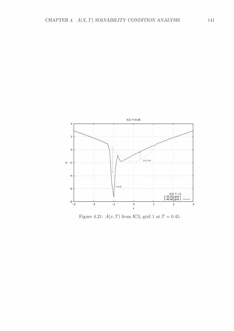
CHAPTER 4. A(X, T ) SOLVABILITY CONDITION ANALYSIS 141
−8
−6
−4
−2
0
2
4
−3 −2 −1 0 1 2 3
A
x
IC3: T=0.45
IC3: T = 0[−20,20] grid 1[−40,40] grid 1
IC3: T=0
T=0.45
Figure 4.21: A(x, T ) from IC3, grid 1 at T = 0.45.
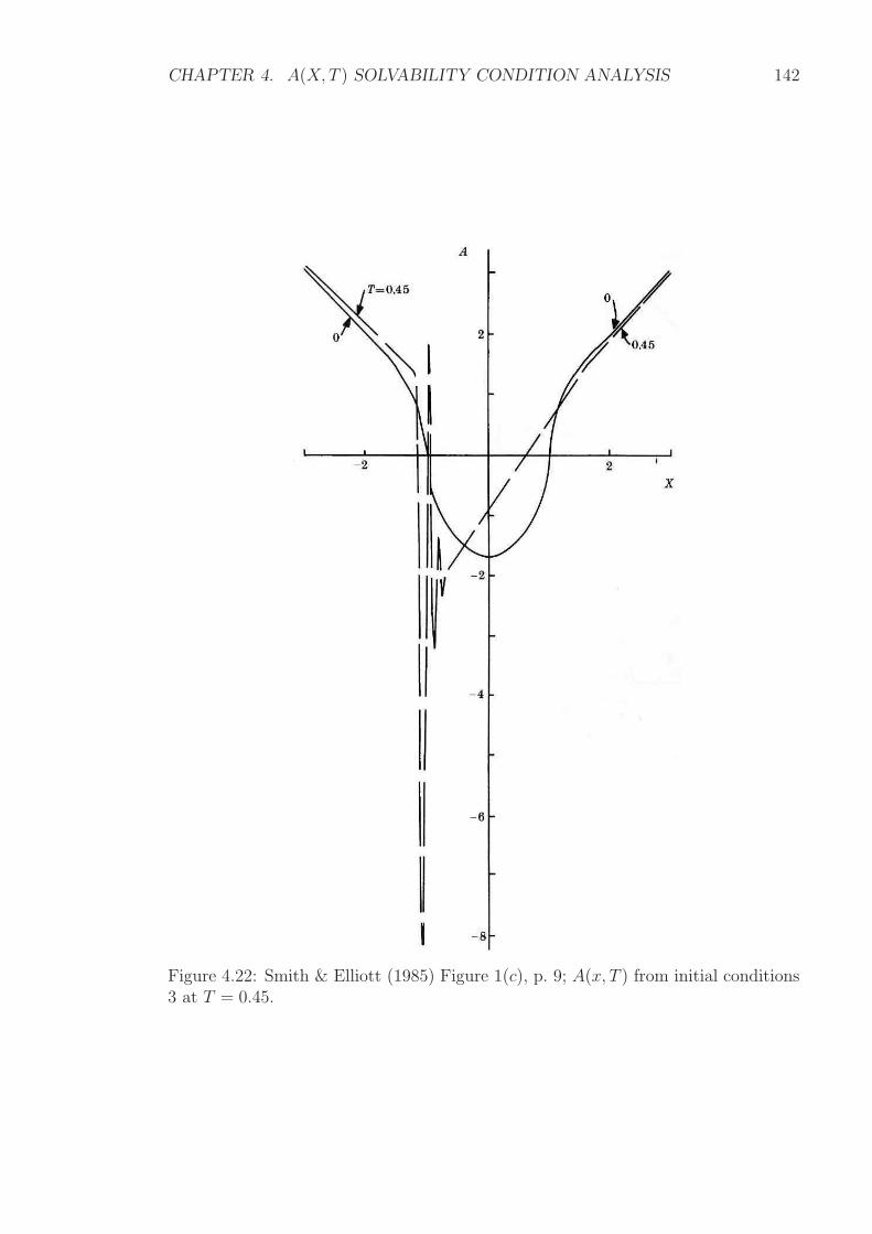
CHAPTER 4. A(X, T ) SOLVABILITY CONDITION ANALYSIS 142
Figure 4.22: Smith & Elliott (1985) Figure 1(c), p. 9; A(x, T ) from initial conditions3 at T = 0.45.
CHAPTER 4. A(X, T ) SOLVABILITY CONDITION ANALYSIS 143
Smith & Elliott (1985) Test Summary
The MATLAB algorithm is working correctly.
1. The error decreases quadratically to zero with each iteration when the iterate
is close to the true solution.
2. The A(x, T ) solutions satisfy the boundary conditions at x = x1, xm+1 and do
not oscillate as the end points are approached.
3. The results from each of the initial conditions IC0, IC1, IC2, IC3 converge to
their A(x, T ) solutions as the number of grid points are increased and step sizes
are decreased. The domains x ∈ [−20, 20] and x ∈ [−40, 40] are sufficiently
large such that the results are also domain independent and depend only on
grid size. However, the results from initial condition IC3 for grid 1 and grid 2
are grid dependent as a breakdown at end time Tend is approached.13
4. The A(x, T ) solutions match those from Smith & Elliott (1985).
4.4 A(x, T ) Algorithm Test
The method used to solve the A(x, T ) equation (4.1) is tested using similar bench-
marks from Section 4.3 such that the MATLAB algorithm for (4.1) is deemed to have
passed the test if all the following conditions are met.
1. The error E (4.17) reduces quadratically towards zero with each iteration when
the iterate is sufficiently close to the solution.
2. The boundary condition (4.6):
A(x, T ) = (|x|2 + 2a(T ))12 , x = x1, xm+1
13The breakdown is discussed in Section 4.5 and investigated further in Chapter 5.
CHAPTER 4. A(X, T ) SOLVABILITY CONDITION ANALYSIS 144
with the angle of attack law (4.3):
a(T ) = 1.331− 1.332e−T ,
is satisfied at all time levels. Moreover, the boundary condition is treated as
a function of x and T and the solution must approach this function smoothly
such that it does not oscillate near the end points.
3. The results converge to true A(x, T ) solutions as the step sizes Dx and DT de-
crease towards zero. Following from Section 4.3, the test grids and the step sizes
are those in Table 4.5. Furthermore, the test spatial domain is x ∈ [−40, 40]
since the size of the domain is sufficiently large such that only the grid affects
the output.
DT Dxgrid 1 0.01 0.1grid 2 0.001 0.05
Table 4.5: Grids and step sizes for implementing the A(x, T ) algorithm test in domainx ∈ [−40, 40].
4.4.1 The Initial Conditions
Initial conditions applied at the start time T = 0 are based on but not identical to the
initial conditions IC0 (4.20), IC1 (4.21), IC2 (4.22) and IC3 (4.23) from the Smith &
Elliott (1985) test in Section 4.3. They take into account a(T ) 6= −0.5 for all time T
but a(T ) is a parameter for the angle of attack law (4.3) between a(0) = −0.001 and
a value slightly above the critical value ac = 1.33 as T →∞.
Initial conditions are directly related to skin friction by (4.2) and represent phys-
ical flow distributions. Thus:
1. Initial condition 0 (abbreviated “IC0”) is
A(x, 0) =√
(x2 − 2a(0)) ; (4.24)
CHAPTER 4. A(X, T ) SOLVABILITY CONDITION ANALYSIS 145
such that skin friction A(x, T ) is initially positive and continuous for all x and
hence, the fluid flow is initially attached along the surface of the airfoil. It
is similar to the boundary condition (4.6). The Smith & Elliott (1985) test
analogy for a(T ) = −0.5 in Section 4.3 leads to a steady state solution.
2. Initial condition 1 (“IC1”) is a small deviation from IC0 (4.24):
A(x, 0) =
√(2.52−2a(0))√
(2.52−2a(0)+0.4)·√
(x2 − 2a(0) + 0.4) , |x| ≤ 2.5
√
(x2 − 2a(0)) , |x| > 2.5 ;
(4.25)
and like IC0, the fluid flow is initially attached along the airfoil.
3. Initial condition 2 (“IC2”) is
A(x, 0) =
1.25|x| , |x| ≤ 0.1√
(x2 − 2a(0)) , |x| > 0.1 ;(4.26)
such that there is point of zero skin friction on the surface. It is similar to the
skin friction for the Ruban (1981) singular solution.
4. Initial condition 3 (“IC3”) is
A(x, 0) =
−1.8 cos(
π2x)
, |x| ≤ 1√(x2
m+1−2a(0))√(x2
m+1−1)·√
(x2 − 1) , |x| > 1 ;(4.27)
where xm+1 is the positive end of the domain. A bubble of reversed flow is
assumed to have formed on the surface where A(x, 0) ≤ 0.
Test Results for Error E
The maximum time for calculations to take place is T = 6. In fact, a breakdown in
the solution is approached as a(T )→ 1.33+ and there is no convergence of Newton’s
method within the maximum number of 50 iterations after a critical point in time
Tend. (See Table 4.6.) Furthermore, the singularity affects Newton’s method. As the
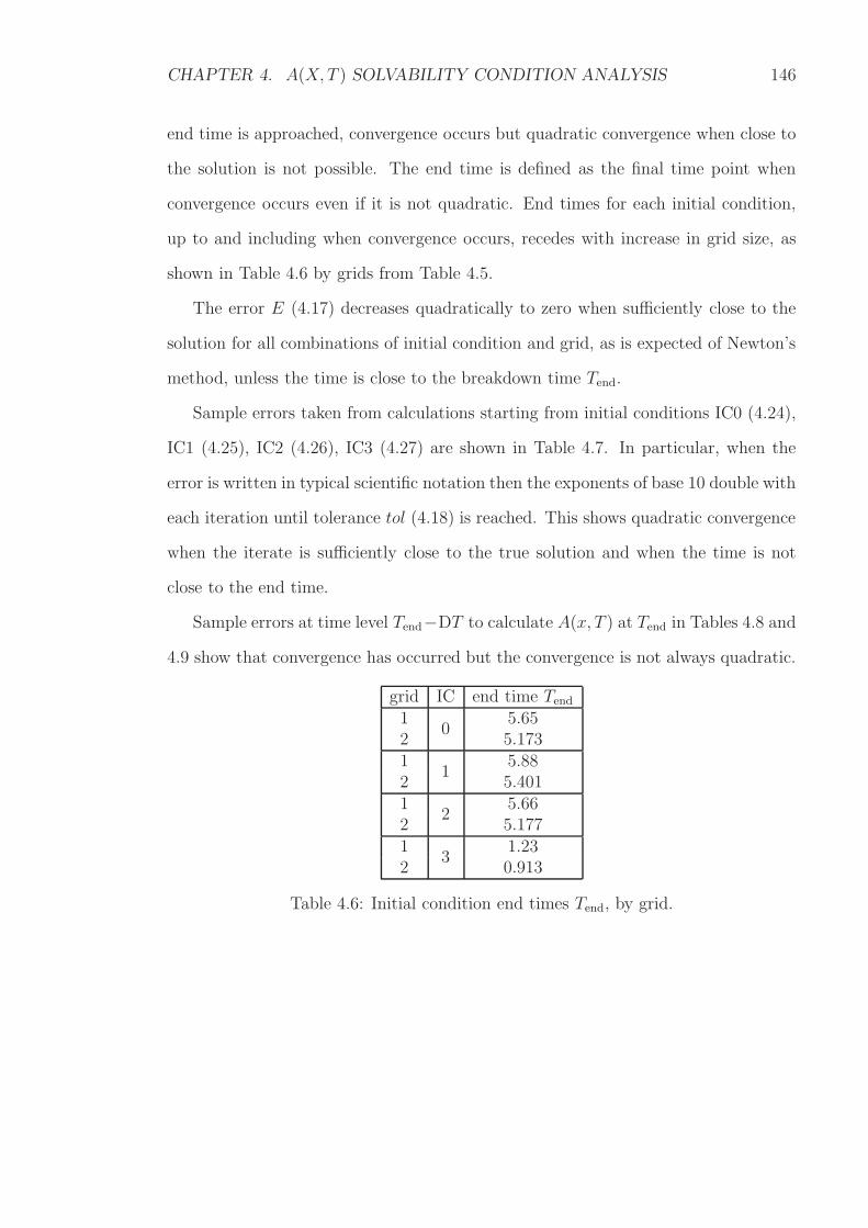
CHAPTER 4. A(X, T ) SOLVABILITY CONDITION ANALYSIS 146
end time is approached, convergence occurs but quadratic convergence when close to
the solution is not possible. The end time is defined as the final time point when
convergence occurs even if it is not quadratic. End times for each initial condition,
up to and including when convergence occurs, recedes with increase in grid size, as
shown in Table 4.6 by grids from Table 4.5.
The error E (4.17) decreases quadratically to zero when sufficiently close to the
solution for all combinations of initial condition and grid, as is expected of Newton’s
method, unless the time is close to the breakdown time Tend.
Sample errors taken from calculations starting from initial conditions IC0 (4.24),
IC1 (4.25), IC2 (4.26), IC3 (4.27) are shown in Table 4.7. In particular, when the
error is written in typical scientific notation then the exponents of base 10 double with
each iteration until tolerance tol (4.18) is reached. This shows quadratic convergence
when the iterate is sufficiently close to the true solution and when the time is not
close to the end time.
Sample errors at time level Tend−DT to calculate A(x, T ) at Tend in Tables 4.8 and
4.9 show that convergence has occurred but the convergence is not always quadratic.
grid IC end time Tend1
05.65
2 5.1731
15.88
2 5.4011
25.66
2 5.1771
31.23
2 0.913
Table 4.6: Initial condition end times Tend, by grid.
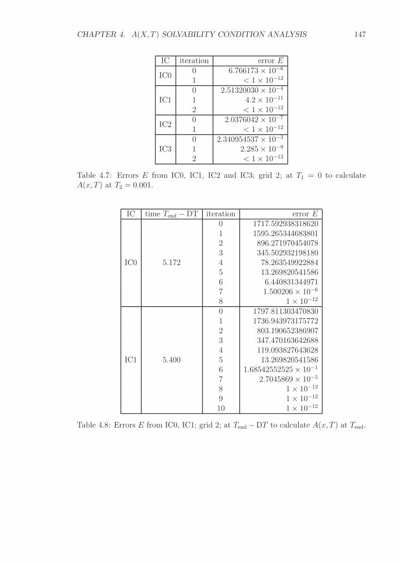
CHAPTER 4. A(X, T ) SOLVABILITY CONDITION ANALYSIS 147
IC iteration error E
IC00 6.766173× 10⁻⁶
1 < 1× 10⁻¹²
IC10 2.51320030× 10⁻⁴
1 4.2× 10⁻¹¹
2 < 1× 10⁻¹²
IC20 2.0376042× 10⁻⁷
1 < 1× 10⁻¹²
IC30 2.340954537× 10⁻³
1 2.285× 10⁻⁹
2 < 1× 10⁻¹²
Table 4.7: Errors E from IC0, IC1, IC2 and IC3; grid 2; at T1 = 0 to calculateA(x, T ) at T2 = 0.001.
IC time Tend −DT iteration error E
IC0 5.172
0 1717.5929383186201 1595.2653446838012 896.2719704540783 345.5029321981804 78.2635499228845 13.2698205415866 6.4408313449717 1.500206× 10⁻⁶
8 1× 10⁻¹²
IC1 5.400
0 1797.8113034708301 1736.9439731757722 803.1906523869073 347.4701636426884 119.0938276436285 13.2698205415866 1.68542552525× 10⁻¹
7 2.7045869× 10⁻⁵
8 1× 10⁻¹²
9 1× 10⁻¹²
10 1× 10⁻¹²
Table 4.8: Errors E from IC0, IC1; grid 2; at Tend−DT to calculate A(x, T ) at Tend.
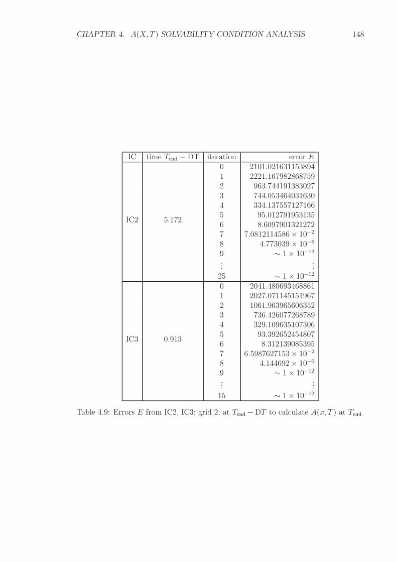
CHAPTER 4. A(X, T ) SOLVABILITY CONDITION ANALYSIS 148
IC time Tend − DT iteration error E
IC2 5.172
0 2101.0216311538941 2221.1679828687592 963.7441913830273 744.0534640316304 334.1375571271665 95.0127919531356 8.60979013212727 7.0812114586× 10⁻²
8 4.773039× 10⁻⁶
9 ∼ 1× 10⁻¹²
......
25 ∼ 1× 10⁻¹²
IC3 0.913
0 2041.4806934688611 2027.0711451519672 1061.9639656063523 736.4260772687894 329.1096351073065 93.3926524548076 8.3121390853957 6.5987627153× 10⁻²
8 4.144692× 10⁻⁶
9 ∼ 1× 10⁻¹²
......
15 ∼ 1× 10⁻¹²
Table 4.9: Errors E from IC2, IC3; grid 2; at Tend−DT to calculate A(x, T ) at Tend.
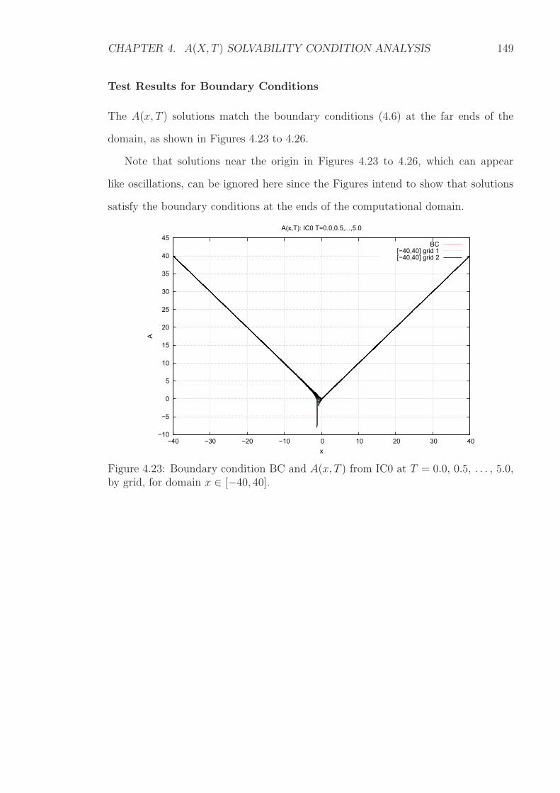
CHAPTER 4. A(X, T ) SOLVABILITY CONDITION ANALYSIS 149
Test Results for Boundary Conditions
The A(x, T ) solutions match the boundary conditions (4.6) at the far ends of the
domain, as shown in Figures 4.23 to 4.26.
Note that solutions near the origin in Figures 4.23 to 4.26, which can appear
like oscillations, can be ignored here since the Figures intend to show that solutions
satisfy the boundary conditions at the ends of the computational domain.
−10
−5
0
5
10
15
20
25
30
35
40
45
−40 −30 −20 −10 0 10 20 30 40
A
x
A(x,T): IC0 T=0.0,0.5,...,5.0
BC[−40,40] grid 1[−40,40] grid 2
Figure 4.23: Boundary condition BC and A(x, T ) from IC0 at T = 0.0, 0.5, . . . , 5.0,by grid, for domain x ∈ [−40, 40].
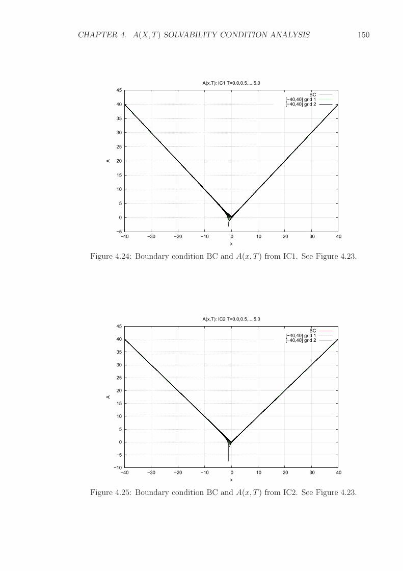
CHAPTER 4. A(X, T ) SOLVABILITY CONDITION ANALYSIS 150
−5
0
5
10
15
20
25
30
35
40
45
−40 −30 −20 −10 0 10 20 30 40
A
x
A(x,T): IC1 T=0.0,0.5,...,5.0
BC[−40,40] grid 1[−40,40] grid 2
Figure 4.24: Boundary condition BC and A(x, T ) from IC1. See Figure 4.23.
−10
−5
0
5
10
15
20
25
30
35
40
45
−40 −30 −20 −10 0 10 20 30 40
A
x
A(x,T): IC2 T=0.0,0.5,...,5.0
BC[−40,40] grid 1[−40,40] grid 2
Figure 4.25: Boundary condition BC and A(x, T ) from IC2. See Figure 4.23.
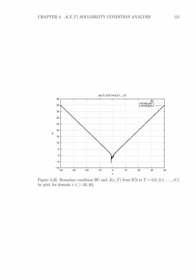
CHAPTER 4. A(X, T ) SOLVABILITY CONDITION ANALYSIS 151
−10
−5
0
5
10
15
20
25
30
35
40
45
−40 −30 −20 −10 0 10 20 30 40
A
x
A(x,T): IC3 T=0.0,0.1,...,0.7
BC[−40,40] grid 1[−40,40] grid 2
Figure 4.26: Boundary condition BC and A(x, T ) from IC3 at T = 0.0, 0.1, . . . , 0.7,by grid, for domain x ∈ [−40, 40].
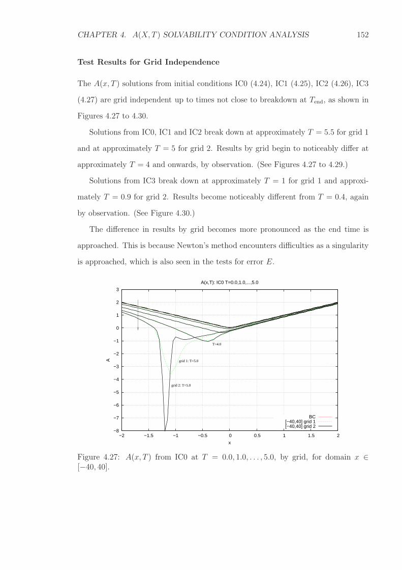
CHAPTER 4. A(X, T ) SOLVABILITY CONDITION ANALYSIS 152
Test Results for Grid Independence
The A(x, T ) solutions from initial conditions IC0 (4.24), IC1 (4.25), IC2 (4.26), IC3
(4.27) are grid independent up to times not close to breakdown at Tend, as shown in
Figures 4.27 to 4.30.
Solutions from IC0, IC1 and IC2 break down at approximately T = 5.5 for grid 1
and at approximately T = 5 for grid 2. Results by grid begin to noticeably differ at
approximately T = 4 and onwards, by observation. (See Figures 4.27 to 4.29.)
Solutions from IC3 break down at approximately T = 1 for grid 1 and approxi-
mately T = 0.9 for grid 2. Results become noticeably different from T = 0.4, again
by observation. (See Figure 4.30.)
The difference in results by grid becomes more pronounced as the end time is
approached. This is because Newton’s method encounters difficulties as a singularity
is approached, which is also seen in the tests for error E.
−8
−7
−6
−5
−4
−3
−2
−1
0
1
2
3
−2 −1.5 −1 −0.5 0 0.5 1 1.5 2
A
x
A(x,T): IC0 T=0.0,1.0,...,5.0
BC[−40,40] grid 1[−40,40] grid 2
grid 1: T=5.0
T=4.0
grid 2: T=5.0
Figure 4.27: A(x, T ) from IC0 at T = 0.0, 1.0, . . . , 5.0, by grid, for domain x ∈[−40, 40].
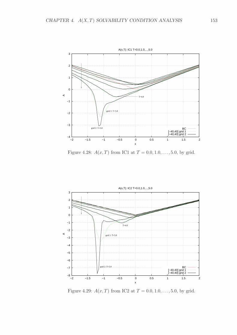
CHAPTER 4. A(X, T ) SOLVABILITY CONDITION ANALYSIS 153
−4
−3
−2
−1
0
1
2
3
−2 −1.5 −1 −0.5 0 0.5 1 1.5 2
A
x
A(x,T): IC1 T=0.0,1.0,...,5.0
BC[−40,40] grid 1[−40,40] grid 2
grid 2: T=5.0
grid 1: T=5.0
T=4.0
Figure 4.28: A(x, T ) from IC1 at T = 0.0, 1.0, . . . , 5.0, by grid.
−8
−7
−6
−5
−4
−3
−2
−1
0
1
2
3
−2 −1.5 −1 −0.5 0 0.5 1 1.5 2
A
x
A(x,T): IC2 T=0.0,1.0,...,5.0
BC[−40,40] grid 1[−40,40] grid 2
grid 2: T=5.0
grid 1: T=5.0
T=4.0
Figure 4.29: A(x, T ) from IC2 at T = 0.0, 1.0, . . . , 5.0, by grid.
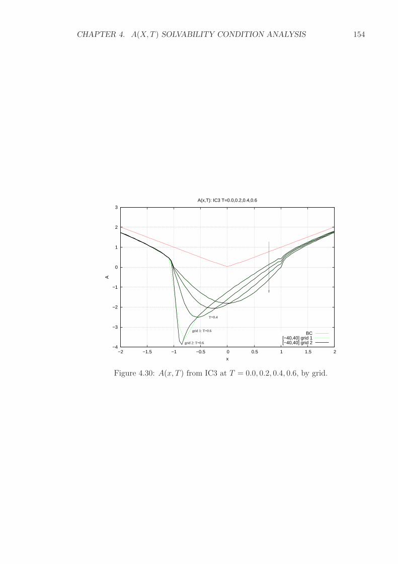
CHAPTER 4. A(X, T ) SOLVABILITY CONDITION ANALYSIS 154
−4
−3
−2
−1
0
1
2
3
−2 −1.5 −1 −0.5 0 0.5 1 1.5 2
A
x
A(x,T): IC3 T=0.0,0.2,0.4,0.6
BC[−40,40] grid 1[−40,40] grid 2grid 2: T=0.6
grid 1: T=0.6
T=0.4
Figure 4.30: A(x, T ) from IC3 at T = 0.0, 0.2, 0.4, 0.6, by grid.
CHAPTER 4. A(X, T ) SOLVABILITY CONDITION ANALYSIS 155
A(x, T ) Algorithm Test Summary
The A(x, T ) algorithm test results are similar to those for the Smith & Elliott (1985)
test in Section 4.3. The MATLAB algorithm is working correctly.
1. The error decreases quadratically to zero with each iteration when the iterate is
close to the true solution until a singularity at the end time Tend is approached.
The steepening singularity causes difficulties for Newton’s method.14
2. The A(x, T ) solutions satisfy the boundary conditions and they do no oscillate
as the end points x = x1 and x = xm+1 are approached.
3. The results from each of the initial conditions IC0, IC1, IC2, IC3 converge to
true solutions for A(x, T ) as the number of grid points are increased and step
sizes are decreased. The domain x ∈ [−40, 40] is sufficiently large such that the
results are dependent only on grid size. In fact, the results for grid 1 and grid 2
are grid independent except until a breakdown at end time Tend is approached.
This is also reflected in the test results for error E.
Similar to the jump in initial condition 3 (4.23) in Section 4.3 and thus the small
wrinkles in solution from the Smith & Elliott (1985) test results, there are also small
wrinkles in the solutions from IC2 (4.26) and from IC3 (4.27) as seen in the grid
independence test Figures 4.29 and 4.30. For IC2, the small wrinkle at x = −2.5
comes directly from a small jump in the crude statement of the initial condition in
MATLAB. For example, IC2:
A(x, 0) =
1.25|x| , |x| ≤ 0.1√
(x2 − 2a(0)) , |x| > 0.1 ;
is written in MATLAB for domain x ∈ [−40, 40], grid 2, as
for j = 2:797;
14The breakdown is discussed in Section 4.5 and investigated further in Chapter 5.
CHAPTER 4. A(X, T ) SOLVABILITY CONDITION ANALYSIS 156
A(j,1) = sqrt(x(j)^2 - 2*O(1));
end
for j = 798:802;
A(j,1) = 1.25*abs(x(j));
end
for j = 803:1600;
A(j,1) = sqrt(x(j)^2 - 2*O(1));
end
where “O” is a(T ). For IC3, the small wrinkle at x = ±1 comes directly from a small
jump in the crude statement of the initial condition in MATLAB. Again, for domain
x ∈ [−40, 40], grid 2, then IC3:
A(x, 0) =
−1.8 cos(
π2x)
, |x| ≤ 1√(x2
m+1−2a(0))√(x2
m+1−1)·√
(x2 − 1) , |x| > 1
is written in MATLAB as
for j = 1:780
A(j,1) = (sqrt(c^2 - 2*O(1))/sqrt(c^2 - 1))*...
sqrt(x(j)^2 - 1);
end
for j = 822:1601
A(j,1) = (sqrt(c^2 - 2*O(1))/sqrt(c^2 - 1))*...
sqrt(x(j)^2 - 1);
end
for j = 781:821
A(j,1) = -1.8*cos((pi/2)*x(j));
end
where “c” is xm+1. However, the wrinkle disturbances from the crude statements of
IC2 and IC3 in MATLAB are small and localised, as shown in Figures 4.29 and 4.30.
CHAPTER 4. A(X, T ) SOLVABILITY CONDITION ANALYSIS 157
Hence, they do not have any significant effect on the solution elsewhere, especially
when compared to the major effects of approaching a breakdown.
4.5 Solutions Close To The Critical Angle
The A(x, T ) solutions for all initial conditions IC0 (4.24), IC1 (4.25) , IC2 (4.26) and
IC3 (4.27) are shown within a region of interest x ∈ [−2, 2] in the Figures.
Solutions for Initial Conditions 0 & 1
From IC0, where the fluid flow is initially attached along the surface of the airfoil in a
similar configuration to the boundary condition (4.6), A(x, T ) has a positive minimum
that is decreasing with time, as shown at intervals of ∆T = 0.5 in Figures 4.31 and
4.32. The A(x, T ) solution becomes very large and negative upstream of x = −0.1
and accelerates to a breakdown at the end time Tend. (See Table 4.10)
From IC1, where the fluid flow is initially attached along the surface but slightly
perturbed from IC0, A(x, T ) has a positive minimum which increases as T → 1 and
shifts downstream from the origin to x ≃ 0.1, as shown at intervals of ∆T = 0.2
in Figure 4.33. The flow structure is attempting to stabilise to a configuration with
no separation. Figure 4.34 shows that between T = 1.2 and T = 1.6, the positive
minimum levels out at x ≃ 0.1 where A ≃ 0.45. From T = 1.6, A(x, T ) decreases
and shifts upstream until the minimum reaches zero at x ≃ −0.1, T ≃ 3.0, as shown
at intervals of ∆T = 0.5 in Figure 4.35. From thereon, A(x, T ) becomes negative
and a closed bubble of reversed flow forms on the surface. The region of reversed
flow becomes more accentuated upstream towards x = −1 with time T until there is
breakdown at end time Tend ≃ 5.5.
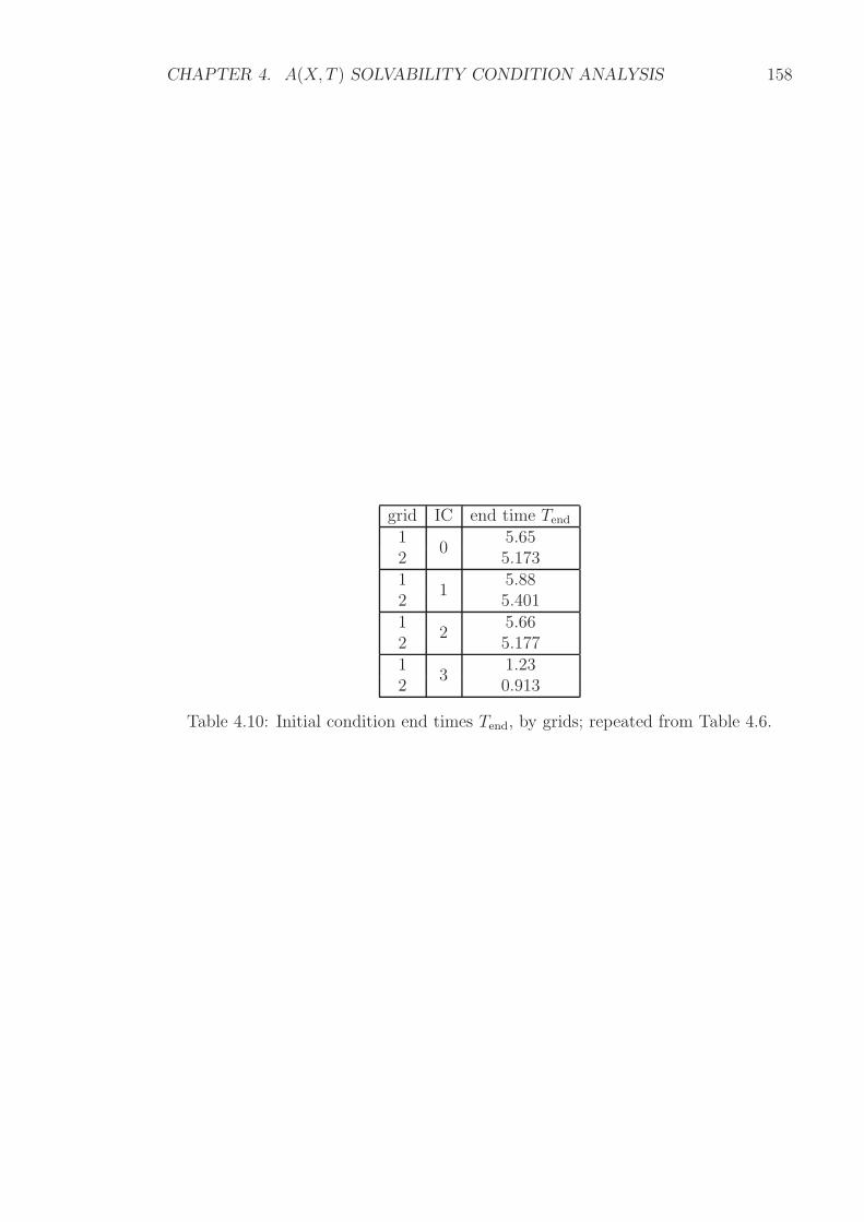
CHAPTER 4. A(X, T ) SOLVABILITY CONDITION ANALYSIS 158
grid IC end time Tend1
05.65
2 5.1731
15.88
2 5.4011
25.66
2 5.1771
31.23
2 0.913
Table 4.10: Initial condition end times Tend, by grids; repeated from Table 4.6.
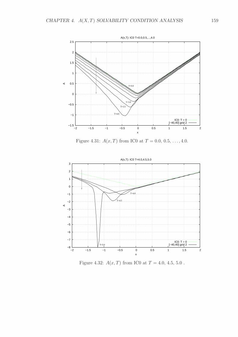
CHAPTER 4. A(X, T ) SOLVABILITY CONDITION ANALYSIS 159
−1.5
−1
−0.5
0
0.5
1
1.5
2
2.5
−2 −1.5 −1 −0.5 0 0.5 1 1.5 2
A
x
A(x,T): IC0 T=0.0,0.5,...,4.0
IC0: T = 0[−40,40] grid 2
T=0.0
T=3.0
T=3.5
T=4.0
Figure 4.31: A(x, T ) from IC0 at T = 0.0, 0.5, . . . , 4.0.
−8
−7
−6
−5
−4
−3
−2
−1
0
1
2
3
−2 −1.5 −1 −0.5 0 0.5 1 1.5 2
A
x
A(x,T): IC0 T=4.0,4.5,5.0
IC0: T = 0[−40,40] grid 2T=5.0
T=4.0
T=4.5
Figure 4.32: A(x, T ) from IC0 at T = 4.0, 4.5, 5.0 .
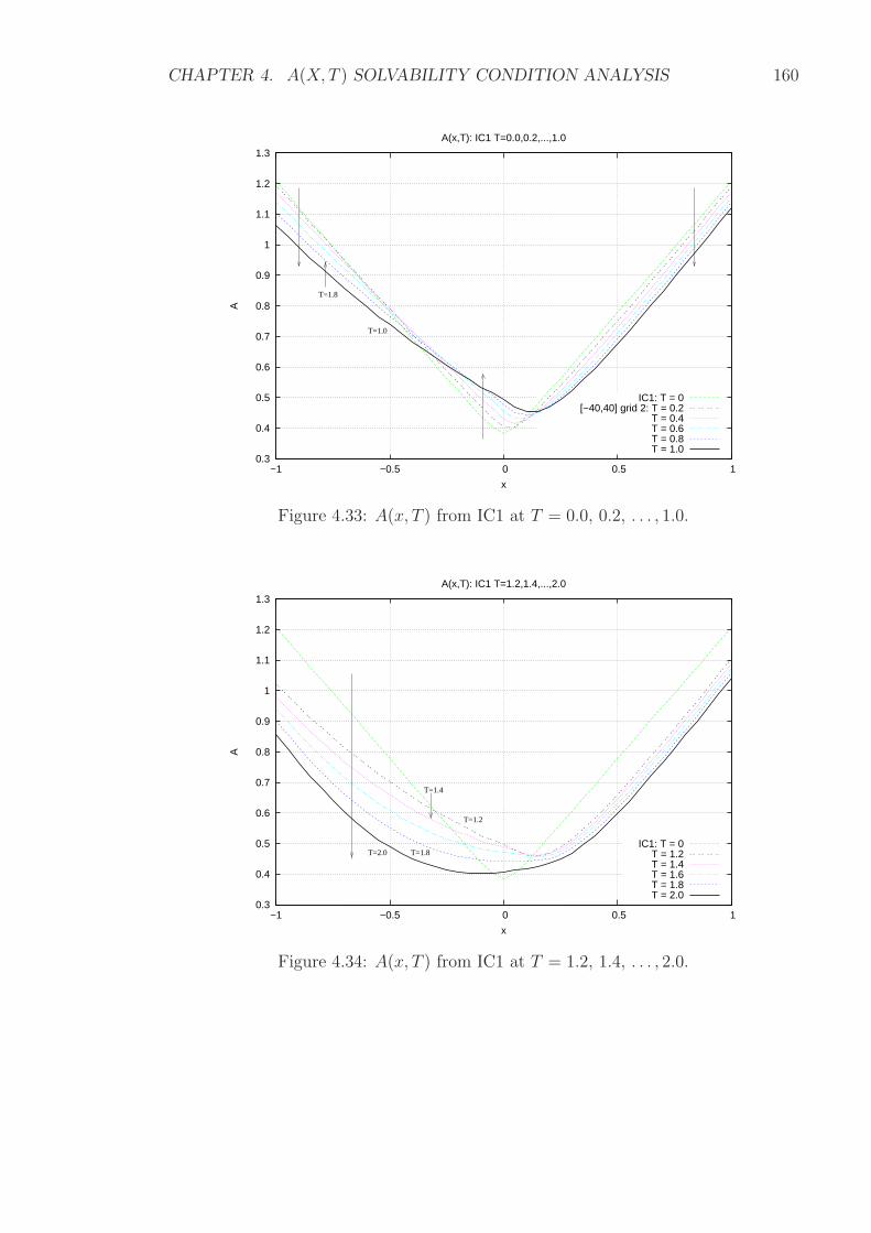
CHAPTER 4. A(X, T ) SOLVABILITY CONDITION ANALYSIS 160
0.3
0.4
0.5
0.6
0.7
0.8
0.9
1
1.1
1.2
1.3
−1 −0.5 0 0.5 1
A
x
A(x,T): IC1 T=0.0,0.2,...,1.0
IC1: T = 0[−40,40] grid 2: T = 0.2
T = 0.4T = 0.6T = 0.8T = 1.0
T=1.8
T=1.0
Figure 4.33: A(x, T ) from IC1 at T = 0.0, 0.2, . . . , 1.0.
0.3
0.4
0.5
0.6
0.7
0.8
0.9
1
1.1
1.2
1.3
−1 −0.5 0 0.5 1
A
x
A(x,T): IC1 T=1.2,1.4,...,2.0
IC1: T = 0T = 1.2T = 1.4T = 1.6T = 1.8T = 2.0
T=1.2
T=1.4
T=1.8T=2.0
Figure 4.34: A(x, T ) from IC1 at T = 1.2, 1.4, . . . , 2.0.
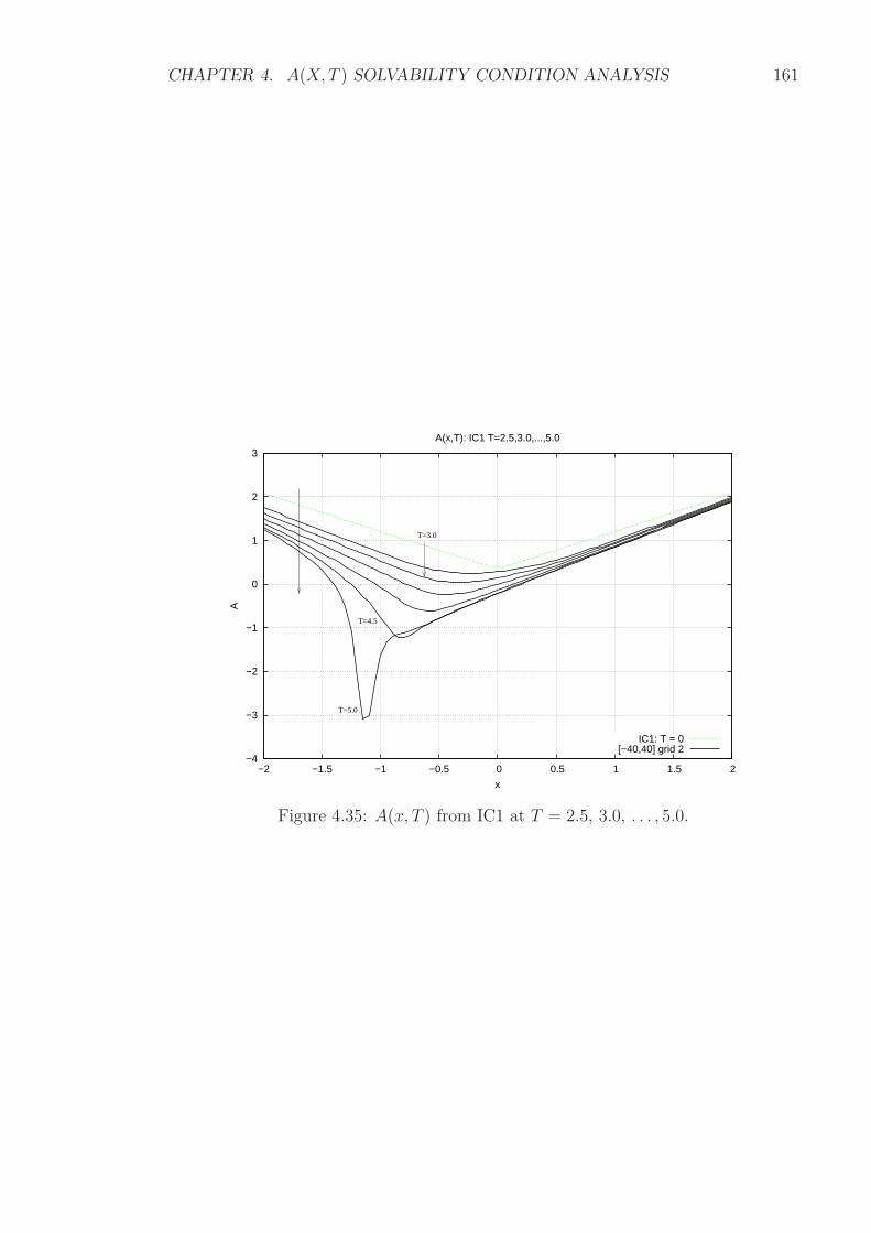
CHAPTER 4. A(X, T ) SOLVABILITY CONDITION ANALYSIS 161
−4
−3
−2
−1
0
1
2
3
−2 −1.5 −1 −0.5 0 0.5 1 1.5 2
A
x
A(x,T): IC1 T=2.5,3.0,...,5.0
IC1: T = 0[−40,40] grid 2
T=5.0
T=4.5
T=3.0
Figure 4.35: A(x, T ) from IC1 at T = 2.5, 3.0, . . . , 5.0.
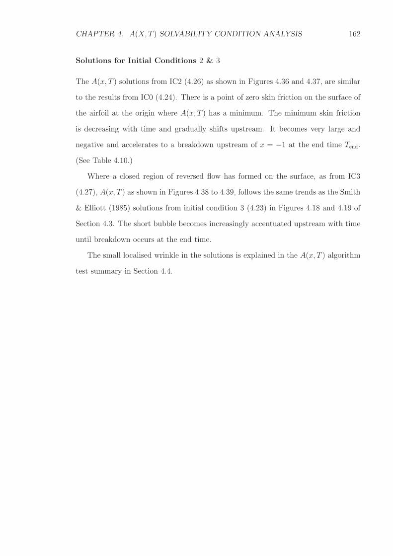
CHAPTER 4. A(X, T ) SOLVABILITY CONDITION ANALYSIS 162
Solutions for Initial Conditions 2 & 3
The A(x, T ) solutions from IC2 (4.26) as shown in Figures 4.36 and 4.37, are similar
to the results from IC0 (4.24). There is a point of zero skin friction on the surface of
the airfoil at the origin where A(x, T ) has a minimum. The minimum skin friction
is decreasing with time and gradually shifts upstream. It becomes very large and
negative and accelerates to a breakdown upstream of x = −1 at the end time Tend.
(See Table 4.10.)
Where a closed region of reversed flow has formed on the surface, as from IC3
(4.27), A(x, T ) as shown in Figures 4.38 to 4.39, follows the same trends as the Smith
& Elliott (1985) solutions from initial condition 3 (4.23) in Figures 4.18 and 4.19 of
Section 4.3. The short bubble becomes increasingly accentuated upstream with time
until breakdown occurs at the end time.
The small localised wrinkle in the solutions is explained in the A(x, T ) algorithm
test summary in Section 4.4.
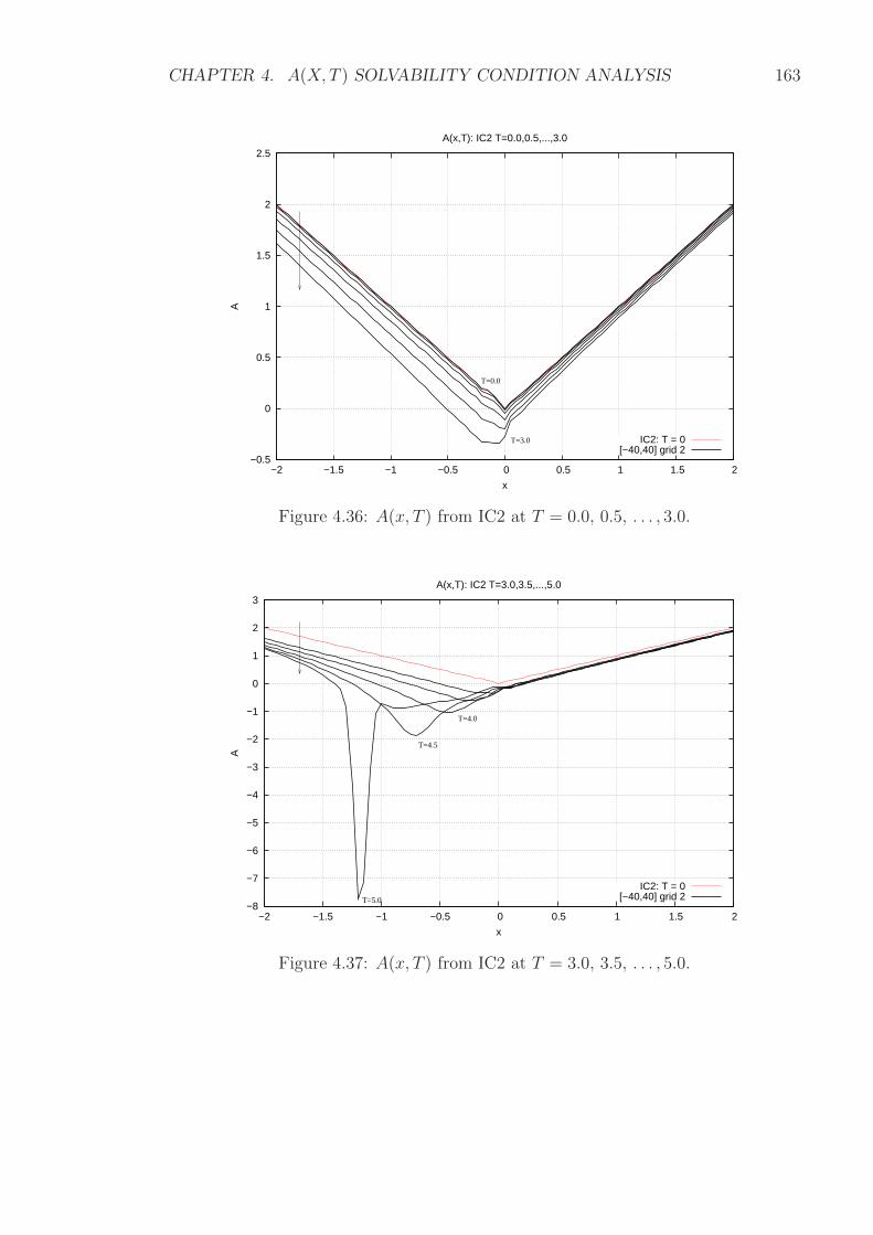
CHAPTER 4. A(X, T ) SOLVABILITY CONDITION ANALYSIS 163
−0.5
0
0.5
1
1.5
2
2.5
−2 −1.5 −1 −0.5 0 0.5 1 1.5 2
A
x
A(x,T): IC2 T=0.0,0.5,...,3.0
IC2: T = 0[−40,40] grid 2
T=0.0
T=3.0
Figure 4.36: A(x, T ) from IC2 at T = 0.0, 0.5, . . . , 3.0.
−8
−7
−6
−5
−4
−3
−2
−1
0
1
2
3
−2 −1.5 −1 −0.5 0 0.5 1 1.5 2
A
x
A(x,T): IC2 T=3.0,3.5,...,5.0
IC2: T = 0[−40,40] grid 2
T=4.0
T=4.5
T=5.0
Figure 4.37: A(x, T ) from IC2 at T = 3.0, 3.5, . . . , 5.0.
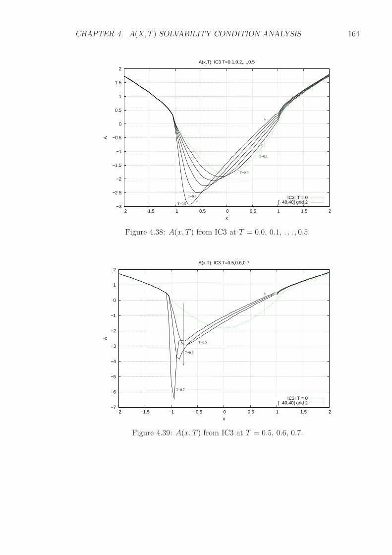
CHAPTER 4. A(X, T ) SOLVABILITY CONDITION ANALYSIS 164
−3
−2.5
−2
−1.5
−1
−0.5
0
0.5
1
1.5
2
−2 −1.5 −1 −0.5 0 0.5 1 1.5 2
A
x
A(x,T): IC3 T=0.1,0.2,...,0.5
IC3: T = 0[−40,40] grid 2
T=0.1
T=0.0
T=0.4
T=0.5
Figure 4.38: A(x, T ) from IC3 at T = 0.0, 0.1, . . . , 0.5.
−7
−6
−5
−4
−3
−2
−1
0
1
2
−2 −1.5 −1 −0.5 0 0.5 1 1.5 2
A
x
A(x,T): IC3 T=0.5,0.6,0.7
IC3: T = 0[−40,40] grid 2
T=0.7
T=0.6
T=0.5
Figure 4.39: A(x, T ) from IC3 at T = 0.5, 0.6, 0.7.
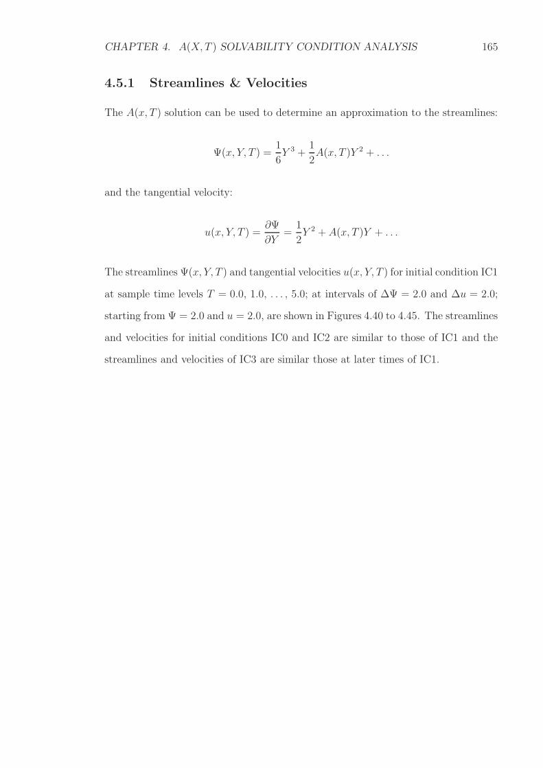
CHAPTER 4. A(X, T ) SOLVABILITY CONDITION ANALYSIS 165
4.5.1 Streamlines & Velocities
The A(x, T ) solution can be used to determine an approximation to the streamlines:
Ψ(x, Y, T ) =1
6Y 3 +
1
2A(x, T )Y 2 + . . .
and the tangential velocity:
u(x, Y, T ) =∂Ψ
∂Y=
1
2Y 2 + A(x, T )Y + . . .
The streamlines Ψ(x, Y, T ) and tangential velocities u(x, Y, T ) for initial condition IC1
at sample time levels T = 0.0, 1.0, . . . , 5.0; at intervals of ∆Ψ = 2.0 and ∆u = 2.0;
starting from Ψ = 2.0 and u = 2.0, are shown in Figures 4.40 to 4.45. The streamlines
and velocities for initial conditions IC0 and IC2 are similar to those of IC1 and the
streamlines and velocities of IC3 are similar those at later times of IC1.
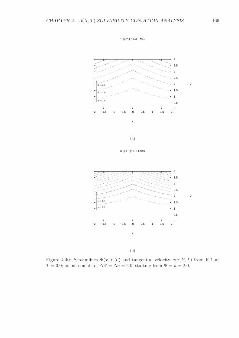
CHAPTER 4. A(X, T ) SOLVABILITY CONDITION ANALYSIS 166
−2 −1.5 −1 −0.5 0 0.5 1 1.5 2 0
0.5
1
1.5
2
2.5
3
3.5
4
Ψ (x,Y,T): IC1 T=0.0
x
Y
Ψ = 2.0
Ψ = 4.0
Ψ = 6.0
(a)
−2 −1.5 −1 −0.5 0 0.5 1 1.5 2 0
0.5
1
1.5
2
2.5
3
3.5
4
u (x,Y,T): IC1 T=0.0
x
Y
u = 4.0
u = 2.0
(b)
Figure 4.40: Streamlines Ψ(x, Y, T ) and tangential velocity u(x, Y, T ) from IC1 atT = 0.0; at increments of ∆Ψ = ∆u = 2.0; starting from Ψ = u = 2.0.

CHAPTER 4. A(X, T ) SOLVABILITY CONDITION ANALYSIS 167
−2 −1.5 −1 −0.5 0 0.5 1 1.5 2 0
0.5
1
1.5
2
2.5
3
3.5
4
Ψ (x,Y,T): IC1 T=1.0
x
Y
Ψ = 2.0
Ψ = 4.0
Ψ = 6.0
(a)
−2 −1.5 −1 −0.5 0 0.5 1 1.5 2 0
0.5
1
1.5
2
2.5
3
3.5
4
u (x,Y,T): IC1 T=1.0
x
Y
u = 2.0
u = 4.0
(b)
Figure 4.41: Ψ(x, Y, T ) and u(x, Y, T ) from IC1 at T = 1.0. See Figure 4.40.

CHAPTER 4. A(X, T ) SOLVABILITY CONDITION ANALYSIS 168
−2 −1.5 −1 −0.5 0 0.5 1 1.5 2 0
0.5
1
1.5
2
2.5
3
3.5
4
Ψ (x,Y,T): IC1 T=2.0
x
YΨ = 6.0
Ψ = 4.0
Ψ = 2.0
(a)
−2 −1.5 −1 −0.5 0 0.5 1 1.5 2 0
0.5
1
1.5
2
2.5
3
3.5
4
u (x,Y,T): IC1 T=2.0
x
Y
u = 2.0
u = 4.0
(b)
Figure 4.42: Ψ(x, Y, T ) and u(x, Y, T ) from IC1 at T = 2.0. See Figure 4.40.

CHAPTER 4. A(X, T ) SOLVABILITY CONDITION ANALYSIS 169
−2 −1.5 −1 −0.5 0 0.5 1 1.5 2 0
0.5
1
1.5
2
2.5
3
3.5
4
Ψ (x,Y,T): IC1 T=3.0
x
Y
Ψ = 2.0
Ψ = 4.0
(a)
−2 −1.5 −1 −0.5 0 0.5 1 1.5 2 0
0.5
1
1.5
2
2.5
3
3.5
4
u (x,Y,T): IC1 T=3.0
x
Y
u = 2.0
u = 4.0
(b)
Figure 4.43: Ψ(x, Y, T ) and u(x, Y, T ) from IC1 at T = 3.0. See Figure 4.40.
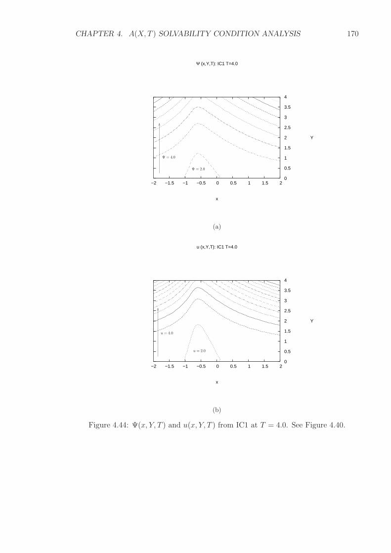
CHAPTER 4. A(X, T ) SOLVABILITY CONDITION ANALYSIS 170
−2 −1.5 −1 −0.5 0 0.5 1 1.5 2 0
0.5
1
1.5
2
2.5
3
3.5
4
Ψ (x,Y,T): IC1 T=4.0
x
Y
Ψ = 2.0
Ψ = 4.0
(a)
−2 −1.5 −1 −0.5 0 0.5 1 1.5 2 0
0.5
1
1.5
2
2.5
3
3.5
4
u (x,Y,T): IC1 T=4.0
x
Y
u = 2.0
u = 4.0
(b)
Figure 4.44: Ψ(x, Y, T ) and u(x, Y, T ) from IC1 at T = 4.0. See Figure 4.40.
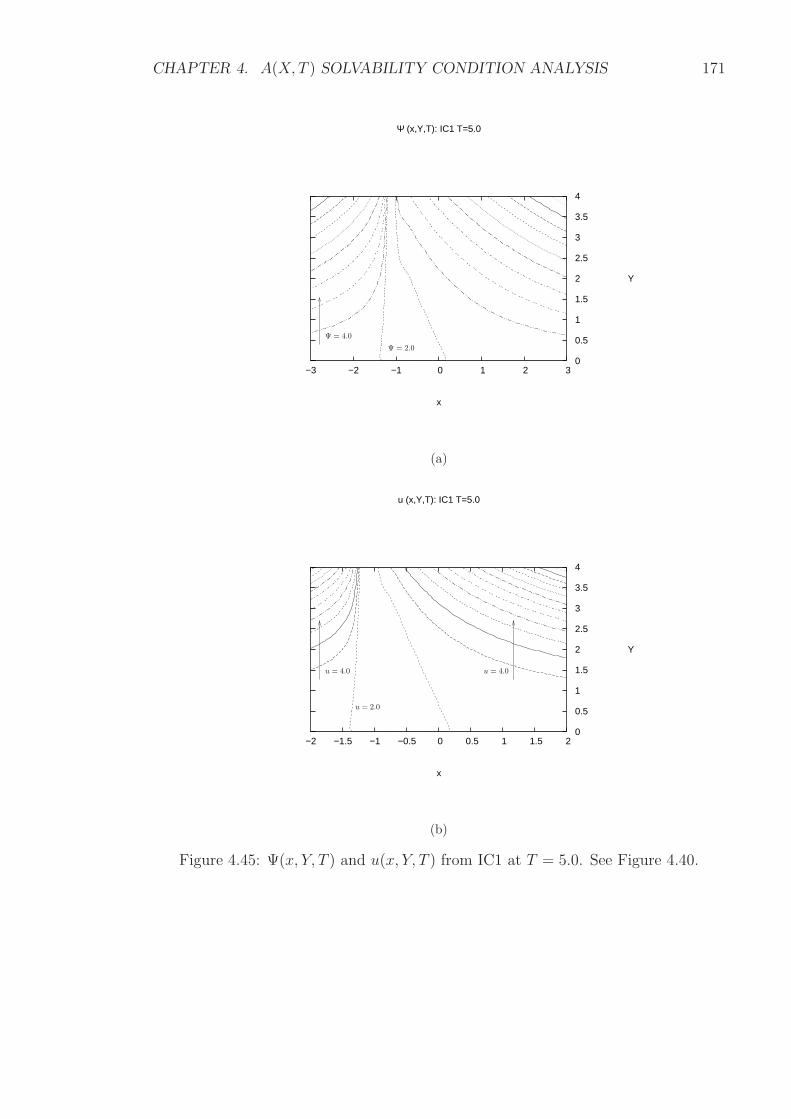
CHAPTER 4. A(X, T ) SOLVABILITY CONDITION ANALYSIS 171
−3 −2 −1 0 1 2 3 0
0.5
1
1.5
2
2.5
3
3.5
4
Ψ (x,Y,T): IC1 T=5.0
x
Y
Ψ = 2.0
Ψ = 4.0
(a)
−2 −1.5 −1 −0.5 0 0.5 1 1.5 2 0
0.5
1
1.5
2
2.5
3
3.5
4
u (x,Y,T): IC1 T=5.0
x
Y
u = 2.0
u = 4.0u = 4.0
(b)
Figure 4.45: Ψ(x, Y, T ) and u(x, Y, T ) from IC1 at T = 5.0. See Figure 4.40.
CHAPTER 4. A(X, T ) SOLVABILITY CONDITION ANALYSIS 172
4.5.2 Singularity & Skin Friction
The flow starting from any type of initial condition, whether the flow is initially
attached along the entire surface of the airfoil, as in IC0 (4.24) and IC1 (4.25); the
flow has a point of zero skin friction on the airfoil, as in IC2 (4.26); or there is a short
bubble of reversed flow on the surface of the airfoil, as in IC3 (4.27); is unstable. The
angle of attack of the airfoil is changing slowly on the large time scale T according to
the law (4.3), as shown in Figure 4.1, so a steady state flow configuration is counter
intuitive.
A singularity is approached as time increases. The singularity is a physical phe-
nomenon as opposed to being a solely numerical method breakdown because it ap-
pears across all grids in Table 4.5, within a small neighbourhood about the point
x = −1 and at approximately the same end time Tend in Table 4.10 for attached flow
and point of zero skin friction initial conditions IC0, IC1 and IC2.
A short bubble of reversed flow will eventually form on the surface of the airfoil
at approximately T = 1.5 from IC0, T = 2.0 from IC1 and almost immediately from
IC2. Recall that when A > 0, the skin friction defined by (4.2) is positive and hence
the fluid is travelling in the direction of the current along the surface of the airfoil.
Analogously, when A < 0, the skin friction is negative and the fluid is travelling
against the current. A point of zero skin friction, when A = 0, first occurs at the
upstream end of the bubble and will recede upstream with time. The downstream
end of the bubble, also where A = 0, is a closing point of the bubble of reversed flow.
The bubble grows in length and volume until a singularity in reached at the end time
Tend, when it bursts. When a bubble has already formed, as in initial condition IC3,
the end time occurs sooner than those for IC0, IC1 and IC2 because the bubble is
already accelerating in growth towards the breakdown.
From all initial conditions, the flow accelerates towards the breakdown despite the
fact that change in angle of attack of the airfoil decelerates with time. This suggests
the breakdown is a runaway process, occurring on even shorter time and length scales,

CHAPTER 4. A(X, T ) SOLVABILITY CONDITION ANALYSIS 173
and the flow configurations are unstable.

Chapter 5
The Nonlinear Breakdown
The slow perturbations, from the small change in angle of attack, to the stream
function solutions of the boundary layer occur on a larger time scale (2.13):
T = σ−1t = O(1) , σ →∞
than the external inviscid flow time scale t. The small change in angle of attack is
represented by asymmetry parameter:
∆k = k(T )− k0 → 0 .
The boundary layer is of length scale (2.12):
s = x− xs = O(1) .
On shorter length and time scales (3.8):
(−s) = O(
σ−4)
, ∆k = O(
σ−8)
, O(σ) > O(
Re120
)
; Re , σ →∞
is the interaction region where induced pressure gradient is negligible. Any viscous-
inviscid interaction between the boundary layer and the external inviscid flow, and the
174
CHAPTER 5. THE NONLINEAR BREAKDOWN 175
subsequent formation of the interaction region can be considered as a first interactive
stage.
The flow structure of the interaction region holds for true skin friction A(x, T )
solutions of the solvability condition. As time increases, there is the formation a short
bubble containing reversed recirculating flow, where skin friction A(x, T ) ≤ 0. The
bubble growth accelerates with time, which is indicated by A(x, T ) also growing large
and negative. The bubble erupts after a finite terminal time Tend and a singularity
of A(x, T ) is reached.
Prior to the singularity, nonlinear breakdown occurs. Nonlinear breakdown can be
considered as a second interactive stage on an even smaller and faster time scale than
the first interactive stage. The second interactive stage is the developing eruption of
the bubble of reversed flow, which causes the boundary layer to thicken.1 Analysis
of the second interactive stage shows that discontinuous skin friction solutions in the
style of Heaviside function waves exist.
On even shorter time and length scales than the nonlinear breakdown, as T →
Tend, a fully unsteady third interactive stage comes into action. The third interactive
stage is the creation and unsteady development of a vortex spanning the thickened
boundary layer at the leading edge, that is eventually shed from the airfoil. Dynamic
stall occurs as the vortex travels from leading edge of the airfoil to the trailing edge
and is then ejected.2 Thus, nonlinear breakdown initiates leading edge stall.
5.1 The Quasi-Steady Second Interactive Stage
The singularity is assumed to occur at the end time Tend = Ts at the point x = Xs
(which is not to be confused with the point of zero skin friction x = xs). Furthermore,
there is a region X of the quasi-steady second interactive stage about the point of
singularity. It is contained within the first interactive stage interaction region such
1A numerical solution of the second interactive stage for fully unsteady boundary layer separationin Lagrangian coordinates is found by Cassel et al. (1996).
2See for example, Cassel (2000); where also, the terminology originates for interactive stages.The third interactive stage is beyond the thesis.
CHAPTER 5. THE NONLINEAR BREAKDOWN 176
that the coordinate x for the interaction region is written as3
x = Xs + (Ts − T )βX , X = O(1) , T → Ts , β > 0 . (5.1)
The second interactive region decays at a rate of order of magnitude (Ts − T )β as
T → Ts and then, on an even shorter time scale before the singularity at Ts, the third
interactive stage of vortex formation and shedding takes over. The second interactive
region is described by the similarity variable
X =(x−Xs)
(Ts − T )β= O(1) , T → Ts , β > 0 (5.2)
where the origin of the second interactive region X = 0 coincides with the point of
singularity x = Xs. The eigenvalue β (which is not to be confused with the eigenvalue
from Section 2.4 or the exponent from Section 2.6.2), is to be found in the analysis.
The point of zero skin friction x = xs is assumed to be travelling within the second
interactive region towards the point of singularity, at a rate of order of magnitude
(Ts − T )α, such that
Xs = xs + C(Ts − T )α , T → Ts , α > 0 . (5.3)
The constant C is arbitrary but related to the speed of travel of the point of zero skin
friction and the direction of travel, depending on its sign. The constant α (which
is not to be confused with the eigenvalue from Section 2.3 or the exponent from
Section 2.6.1) is also arbitrary except 0 < α ≤ β such that the point of zero skin
friction is travelling towards the point of singularity at a slower rate than the second
interactive region is decaying about it. The second interactive region is then an intact
structure which does not destroy the interaction region from Chapters 3 and 4. (See
Figure 5.1.)
Therefore, the first interactive stage interaction region with coordinate x (5.1)
3See also for example, Cassel et al. (1996).
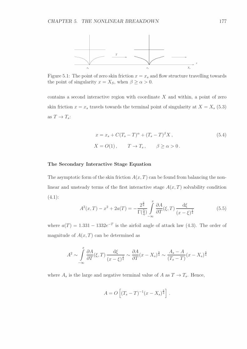
CHAPTER 5. THE NONLINEAR BREAKDOWN 177
Xs
x
xs xs
T
Figure 5.1: The point of zero skin friction x = xs and flow structure travelling towardsthe point of singularity x = XS, when β ≥ α > 0.
contains a second interactive region with coordinate X and within, a point of zero
skin friction x = xs travels towards the terminal point of singularity at X = Xs (5.3)
as T → Ts:
x = xs + C(Ts − T )α + (Ts − T )βX , (5.4)
X = O(1) , T → Ts , β ≥ α > 0 .
The Secondary Interactive Stage Equation
The asymptotic form of the skin friction A(x, T ) can be found from balancing the non-
linear and unsteady terms of the first interactive stage A(x, T ) solvability condition
(4.1):
A2(x, T )− x2 + 2a(T ) = − 234
Γ(54)
x∫
−∞
∂A
∂T(ξ, T )
dξ
(x− ξ) 14
(5.5)
where a(T ) = 1.331 − 1332e−T is the airfoil angle of attack law (4.3). The order of
magnitude of A(x, T ) can be determined as
A2 ∼x∫
−∞
∂A
∂T(ξ, T )
dξ
(x− ξ) 14
∼ ∂A
∂T(x−Xs)
34 ∼ As − A
(Ts − T )(x−Xs)
34
where As is the large and negative terminal value of A as T → Ts. Hence,
A = O[
(Ts − T )−1(x−Xs)34
]
.
CHAPTER 5. THE NONLINEAR BREAKDOWN 178
Therefore, taking into account the x and T relation 5.4 where x−Xs = (Ts − T )βX
and Xs = xs + C(Ts − T )α, the skin friction A(x, T ) series expansion of the second
interactive region arises in the form:
A(x, T ) = (Ts − T )34n−1A(X) + . . . A(X) = O(1) . (5.6)
The exponent and eigenvalue n(α, β) is a function of α and β with
0 < n <4
3(5.7)
in order for 34n − 1 < 0 and |A(x, T )| to be large during the nonlinear breakdown
process. The eigenvalue n is to be determined during the analysis.
Additionally, as A(x, T ) becomes large compared to x and a(T ) then by (5.5):
A2 ∼(
−x2 + 2a(T ))−1
. (5.8)
The Taylor series expansion of −x2 + 2a(T ) about x = Xs and T = Ts is:
− x2 + 2a(T ) = −X2s + 2a(Ts) + 2(Ts − T )
da
dT(Ts) + (Ts − T )2
d2a
dT 2(Ts) + . . .
then by the order of magnitude of A(x, T ) from (5.6):
− x2 + 2a(T ) = (Ts − T )2−32n(−X2
s + 2a(Ts)) + . . .
The −x2 + 2a(T ) term cannot be balanced with A2 in the second interactive region,
that is the change in angle of attack a(T ) is no longer relevant once A(x, T ) is growing
large and negative towards the nonlinear breakdown. This confirms the runaway
process of nonlinear breakdown and leading edge stall, as first mentioned in Section
4.5.2
The analysis of the second interactive region proceeds. Substitution of the A(x, T )
CHAPTER 5. THE NONLINEAR BREAKDOWN 179
series expansion (5.6) into the A(x, T ) equation (5.5) gives the terms:
A(x, T )2 = (Ts − T )32n−2A2(X) ;
∂A
∂T(x, T ) = (Ts − T )
34n−2
[
−(
3
4n− 1
)]
A(X) + (Ts − T )34n−1 dA
dX(X)
∂X
∂T
= (Ts − T )34n−2
[
−(
3
4n− 1
)]
A(X) + (Ts − T )34n−2 dA
dX(X)βX
+ (Ts − T )34n+α−β−2 dA
dX(X)αC .
By (5.4):
X = (x− xs − C(Ts − T )α) (Ts − T )−β
then
∂X
∂T= αC(Ts − T )α−1 · (Ts − T )−β
+ (x− xs − C(Ts − T )α) · −β(Ts − T )−β−1
= (Ts − T )α−β−1αC
− (x− xs − C(Ts − T )α) (Ts − T )−β · β(Ts − T )−1
= (Ts − T )−1βX + (Ts − T )α−β−1αC ;
and
dx = (Ts − T )βdX ⇒ dξ = (Ts − T )βdX .
Hence, the integral:
x∫
−∞
· dξ
(x− ξ) 14
⇒ (Ts − T )34β
X∫
−∞
· dξ
(X − ξ) 14
CHAPTER 5. THE NONLINEAR BREAKDOWN 180
Therefore, the second interactive region A(X) equation is
(Ts − T )34nA2(X)
= (Ts − T )34β · − 2
34
Γ(54)
X∫
−∞
[
−(
3
4n− 1
)
A(ξ) + βξdA
dξ(ξ)
]
dξ
(X − ξ) 14
+ (Ts − T )α−14β · − 2
34
Γ(54)
X∫
−∞
[
αCdA
dξ(ξ)
]
dξ
(X − ξ) 14
. (5.9)
5.1.1 Second Interactive Flow Configuration
There are three physical flow cases, of which two cases (5.10) and (5.15) arise from
the balance of terms in the second interactive region A(X) equation (5.9), that can
be described by one nonlinear breakdown equation (5.16).
Firstly, if the order of magnitude of the nonlinear term of (5.9) is the same as
that of both integrals on the right hand side, then
3
4n = α− 1
4β =
3
4β ⇐⇒ n = β = α . (5.10)
The point of zero skin friction x = xs is travelling at the same rate at which the
second interactive region is decaying, such that
x = xs + C(Ts − T )β + (Ts − T )βX = xs + (Ts − T )β[X + C] , (5.11)
X = O(1)
and the asymptotic structure of A(x, T ) is:
A(x, T ) = (Ts − T )34β−1A(X) + . . . (5.12)
CHAPTER 5. THE NONLINEAR BREAKDOWN 181
Hence, the second interactive region A(X) equation (5.9) becomes:
A2(X) = − 234
Γ(54)
X∫
−∞
[
−(
3
4β − 1
)
A(ξ) + β(ξ + C)dA
dξ(ξ)
]
dξ
(X − ξ) 14
.
With the Galilean transformation of the variables:
X → X + C , ξ → ξ + C (5.13)
then
x = xs + (Ts − T )βX , X = O(1) (5.14)
and the equation becomes
A2(X) = − 234
Γ(54)
X∫
−∞
[
−(
3
4β − 1
)
A(ξ) + βξdA
dξ(ξ)
]
dξ
(X − ξ) 14
.
The limits of the integral remain unchanged by the linear transformation since X is
arbitrary and the positive end of the computational domain for the numerical method
is expected to be a large and extended towards infinity.
On the other hand, setting C = 0 such that the point of skin friction is stationary
within the observer’s frame of reference also gives the same governing equation.
Secondly, if the order of magnitude of the nonlinear term is the same as that of
the first integral on the right hand side of (5.9) whilst larger in order of magnitude
than the second integral, then
3
4n =
3
4β > α− 1
4β ⇐⇒ n = β > α . (5.15)
The point of zero skin friction is travelling at a slower rate than the second interactive
region is decaying, such that
x = xs + C(Ts − T )α + (Ts − T )βX , X = O(1) .
CHAPTER 5. THE NONLINEAR BREAKDOWN 182
The interaction region flow structure is assumed to remain intact and moves with the
point of zero skin friction, as shown in Figure 5.1. The structure of A(x, T ) is the
same as that for the previous case when n = β = α such that
A(x, T ) = (Ts − T )34β−1A(X) + . . .
Indeed, by the similarity variable (5.2):
X =(x−Xs)
(Ts − T )β=
[x− xs − C(Ts − T )α](Ts − T )β
= O(1) ,
the denominator with eigenvalue β, that is the rate of decay of the region, is the dom-
inant factor as opposed to the travelling speed of the point. The second interactive
region A(X) equation (5.9) becomes
A2(X) = − 234
Γ(54)
X∫
−∞
[
−(
3
4β − 1
)
A(ξ) + βξdA
dξ(ξ)
]
dξ
(X − ξ) 14
+ (Ts − T )(α−β)
− 234
Γ(54)
X∫
−∞
[
αCdA
dξ(ξ)
]
dξ
(X − ξ) 14
As T → Ts, the second integral cannot be balanced with the rest of equation since
the exponent α− β > 0. Hence, the equation is
A2(X) = − 234
Γ(54)
X∫
−∞
[
−(
3
4β − 1
)
A(ξ) + βξdA
dξ(ξ)
]
dξ
(X − ξ) 14
,
which is identical to the equation for the first case when n = β = α and the additional
case of a fixed point of zero skin friction, when C = 0.
The flow involving a moving point of zero skin friction along a wall is closely
related to steady flow when the point of zero skin friction is fixed. The velocity
profiles are transformed to a wall-fixed frame by the Galilean transformation (5.13),
that is by adding or subtracting the constant velocity C. If the point of zero skin
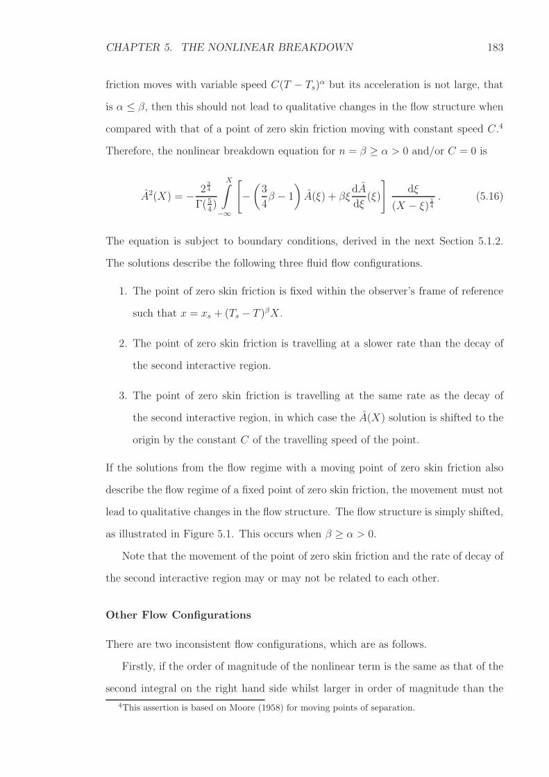
CHAPTER 5. THE NONLINEAR BREAKDOWN 183
friction moves with variable speed C(T − Ts)α but its acceleration is not large, that
is α ≤ β, then this should not lead to qualitative changes in the flow structure when
compared with that of a point of zero skin friction moving with constant speed C.4
Therefore, the nonlinear breakdown equation for n = β ≥ α > 0 and/or C = 0 is
A2(X) = − 234
Γ(54)
X∫
−∞
[
−(
3
4β − 1
)
A(ξ) + βξdA
dξ(ξ)
]
dξ
(X − ξ) 14
. (5.16)
The equation is subject to boundary conditions, derived in the next Section 5.1.2.
The solutions describe the following three fluid flow configurations.
1. The point of zero skin friction is fixed within the observer’s frame of reference
such that x = xs + (Ts − T )βX .
2. The point of zero skin friction is travelling at a slower rate than the decay of
the second interactive region.
3. The point of zero skin friction is travelling at the same rate as the decay of
the second interactive region, in which case the A(X) solution is shifted to the
origin by the constant C of the travelling speed of the point.
If the solutions from the flow regime with a moving point of zero skin friction also
describe the flow regime of a fixed point of zero skin friction, the movement must not
lead to qualitative changes in the flow structure. The flow structure is simply shifted,
as illustrated in Figure 5.1. This occurs when β ≥ α > 0.
Note that the movement of the point of zero skin friction and the rate of decay of
the second interactive region may or may not be related to each other.
Other Flow Configurations
There are two inconsistent flow configurations, which are as follows.
Firstly, if the order of magnitude of the nonlinear term is the same as that of the
second integral on the right hand side whilst larger in order of magnitude than the
4This assertion is based on Moore (1958) for moving points of separation.
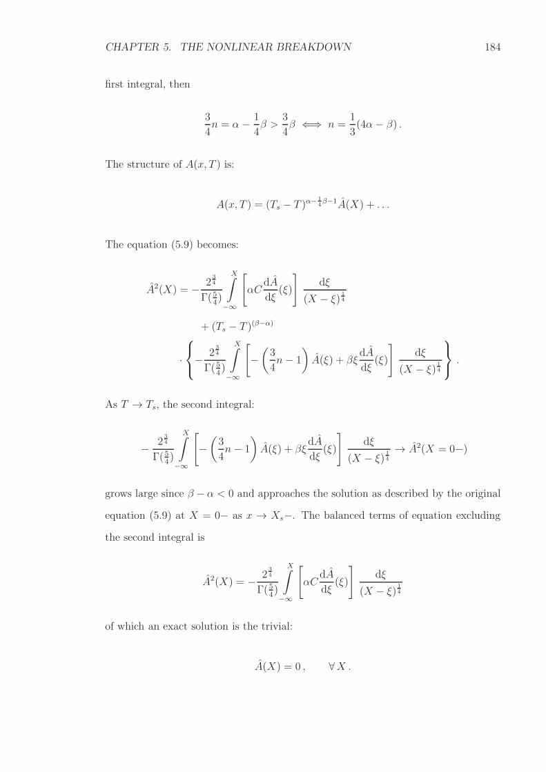
CHAPTER 5. THE NONLINEAR BREAKDOWN 184
first integral, then
3
4n = α− 1
4β >
3
4β ⇐⇒ n =
1
3(4α− β) .
The structure of A(x, T ) is:
A(x, T ) = (Ts − T )α−14β−1A(X) + . . .
The equation (5.9) becomes:
A2(X) = − 234
Γ(54)
X∫
−∞
[
αCdA
dξ(ξ)
]
dξ
(X − ξ) 14
+ (Ts − T )(β−α)
·
− 234
Γ(54)
X∫
−∞
[
−(
3
4n− 1
)
A(ξ) + βξdA
dξ(ξ)
]
dξ
(X − ξ) 14
.
As T → Ts, the second integral:
− 234
Γ(54)
X∫
−∞
[
−(
3
4n− 1
)
A(ξ) + βξdA
dξ(ξ)
]
dξ
(X − ξ) 14
→ A2(X = 0−)
grows large since β − α < 0 and approaches the solution as described by the original
equation (5.9) at X = 0− as x → Xs−. The balanced terms of equation excluding
the second integral is
A2(X) = − 234
Γ(54)
X∫
−∞
[
αCdA
dξ(ξ)
]
dξ
(X − ξ) 14
of which an exact solution is the trivial:
A(X) = 0 , ∀X .
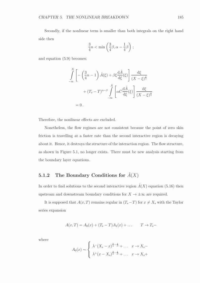
CHAPTER 5. THE NONLINEAR BREAKDOWN 185
Secondly, if the nonlinear term is smaller than both integrals on the right hand
side then
3
4n < min
(
3
4β, α− 1
4β
)
;
and equation (5.9) becomes:
X∫
−∞
[
−(
3
4n− 1
)
A(ξ) + βξdA
dξ(ξ)
]
dξ
(X − ξ) 14
+ (Ts − T )α−β
X∫
−∞
[
αCdA
dξ(ξ)
]
dξ
(X − ξ) 14
= 0 .
Therefore, the nonlinear effects are excluded.
Nonetheless, the flow regimes are not consistent because the point of zero skin
friction is travelling at a faster rate than the second interactive region is decaying
about it. Hence, it destroys the structure of the interaction region. The flow structure,
as shown in Figure 5.1, no longer exists. There must be new analysis starting from
the boundary layer equations.
5.1.2 The Boundary Conditions for A(X)
In order to find solutions to the second interactive region A(X) equation (5.16) then
upstream and downstream boundary conditions for X → ±∞ are required.
It is supposed that A(x, T ) remains regular in (Ts−T ) for x 6= Xs with the Taylor
series expansion
A(x, T ) = A0(x) + (Ts − T )A1(x) + . . . T → Ts−
where
A0(x) ∼
λ−(Xs − x)34− 1
β + . . . x→ Xs−
λ+(x−Xs)34− 1
β + . . . x→ Xs+
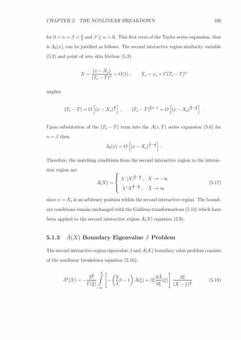
CHAPTER 5. THE NONLINEAR BREAKDOWN 186
for 0 < n = β < 43and β ≥ α > 0. This first term of the Taylor series expansion, that
is A0(x), can be justified as follows. The second interactive region similarity variable
(5.2) and point of zero skin friction (5.3):
X =(x−Xs)
(Ts − T )β= O(1) , Xs = xs + C(Ts − T )α
implies
(Ts − T ) = O[
(x−Xs)1β
]
, (Ts − T )34β−1 = O
[
(x−Xs)34− 1
β
]
.
Upon substitution of the (Ts − T ) term into the A(x, T ) series expansion (5.6) for
n = β then
A0(x) = O[
(x−Xs)34− 1
β
]
.
Therefore, the matching conditions from the second interactive region to the interac-
tion region are
A(X) ∼
λ−|X| 34− 1β , X → −∞
λ+X34− 1
β , X →∞(5.17)
since x = Xs is an arbitrary position within the second interactive region. The bound-
ary conditions remain unchanged with the Galilean transformations (5.13) which have
been applied to the second interactive region A(X) equation (5.9).
5.1.3 A(X) Boundary Eigenvalue β Problem
The second interactive region eigenvalue β and A(X) boundary value problem consists
of the nonlinear breakdown equation (5.16):
A2(X) = − 234
Γ(54)
X∫
−∞
[
−(
3
4β − 1
)
A(ξ) + βξdA
dξ(ξ)
]
dξ
(X − ξ) 14
(5.18)
CHAPTER 5. THE NONLINEAR BREAKDOWN 187
for 0 < n = β < 43and β ≥ α > 0, with the boundary conditions (5.17):
A(X) ∼
λ−|X| 34− 1β , X → −∞
λ+X34− 1
β , X →∞ .(5.19)
Transformation to the Smith & Elliott (1985) Nonlinear Breakdown Prob-
lem
The normalising transformations:
A(X)→(
234
Γ(54)
)1− 34β
A(X) , X →(
234
Γ(54)
)−β
X (5.20)
convert equation (5.18) to the nonlinear breakdown equation by Smith & Elliott
(1985):
A2(X) =
X∫
−∞
[
(
3
4β − 1
)
A(ξ)− βξdAdξ
(ξ)
]
dξ
(X − ξ) 14
. (5.21)
The boundary conditions remain unchanged by the normalising transformations.
The affine transformations:
A(X)→ |λ−| 34βA(X) , X → |λ−|βX (5.22)
convert the boundary conditions (5.19) also to those by Smith & Elliott (1985). When
the affine transformations are applied to the nonlinear breakdown equation, there is
no change. The boundary equations become:
A(X) ∼
λ1|X|34− 1
β , X → −∞
λ2X34− 1
β , X →∞
where λ2 is an arbitrary constant. The boundary value constant λ1 is known to be
either λ1 = +1 for attached forward flow upstream or λ1 = −1 for detached reverse
flow upstream. From Smith & Elliott (1985), where X = X , “it soon became fairly
CHAPTER 5. THE NONLINEAR BREAKDOWN 188
clear that... λ1 = −1 is necessary, since with λ1 = +1 the solution for A always
appeared to blow up eventually in X < 0, in line numerically with the singularity
A ∝ −X1(X1 − X)14 , as X → X1− ,
for X1 negative... This singularity is not removable...” Therefore, the boundary
conditions to solve the nonlinear breakdown equation are:
A(X) ∼
−|X| 34− 1β , X → −∞
λ2X34− 1
β , X →∞(5.23)
where λ2 is a boundary value constant to be found in the course of the solution.
A numerical solution to the boundary eigenvalue β problem for the A(X) equation
(5.21) with boundary conditions (5.23) is given by Smith & Elliott (1985). Neverthe-
less, another numerical solution is found.
5.2 A(X) Equation Numerical Treatment
The boundary eigenvalue problem is solved using the numerical shooting method and
Newton’s method for a system of nonlinear equations with MATLAB. The discreti-
sation of the A(X) equation (5.21) is analogous to the numerical treatment of the
A(x, T ) equation in Section 4.1. From hereon, the notation Xi denotes the value X(i)
of a vector X and Ai denotes A(X(i)) of a vector A.
The computational domain over which the problem is to be solved is discretised
with a uniform grid size DX and m+1 spatial points starting at a large and negative
X1 and extending to a large and positive Xm+1 such that Xi = X1 + (i − 1)DX for
i = 1, 2, . . . , m + 1. The domain is arbitrarily chosen to be large; either [−50, 50],
[−100, 100], [−150, 150], [−200, 200] or [−250, 250]; whilst the step size is one of
DX = 0.4, 0.2, 0.1, 0.05.
The eigenvalue β is an unknown constant except that it is in the range 0 < β < 43
CHAPTER 5. THE NONLINEAR BREAKDOWN 189
and hence, it is reasonable that the problem is solved for each β = 0.01, 0.02, . . . , 1.33,
with the eigenvalue closest to the true value giving the A(X) solution which most
satisfies the criteria for the true solution, as tested in Section 5.3.
A numerical shooting method is used first to determine if solutions exist by solving
for each β = 0.01, 0.02, . . . , 1.33. Secondly, Newton’s method is used to solve the
boundary value problem accurately using the information from the numerical shooting
method as an initial distribution. Both methods are tested in Section 5.3.
Centring
In order to implement either method, the A(X) equation (5.21) is discretised into a
system of m nonlinear equations for m−1 variables from the m+1 total values of Ai
minus the two end point values A1 and Am+1 known from the boundary conditions.
There are m equations for m− 1 variables because there is centring of the A(X)
equation at X = Xi+ 12, where the half-subscript means
Xi+ 12=
1
2(Xi +Xi+1) .
The centring reflects the implicit nature of the problem. Each (i + 1)-th equation
for i = 1, 2, . . . , m solves for Ai and Ai+1 and uses information at the spatial point
X = Xi+1, that is the value of Ai+1 known from an initial distribution, and at all the
points leading up to it from the start of the domain X1. Hence, the X term in the
integrand becomes X = Xi+1.
The left hand side of the (i+ 1)-th equation is centred in space and is discretised
as
A2(X) =1
2
(
A2i + A2
i+1
)
. (5.24)
It is to match with the integral (5.27), with (5.28) and (5.29), on the right hand side
later.
CHAPTER 5. THE NONLINEAR BREAKDOWN 190
The Integral
The integral on the right hand side of the (i+ 1)-th equation is approximated as
X∫
−∞
[
(
3
4β − 1
)
A(ξ)− βξdAdξ
(ξ)
]
dξ
(X − ξ) 14
≃(
3
4β − 1
)
X1∫
−∞
+
X2∫
X1
+ . . .+
Xi+1∫
Xi
A(ξ)dξ
(X − ξ) 14
− β
X1∫
−∞
+
X2∫
X1
+ . . .+
Xi+1∫
Xi
ξdA
dξ(ξ)
dξ
(X − ξ) 14
. (5.25)
The upper limit of the integral and the X term in the integrand stop at the specific
spatial point X = Xi+1. Also, X1 is large and negative, and Xi+1 > X1.
The contribution from the integral between the limits X = −∞ and the large and
negative X = X1, calculated at X = Xi+1, is:
X1∫
−∞
[
(
3
4β − 1
)
A(ξ)− βξdAdξ
(ξ)
]
dξ
(Xi+1 − ξ)14
≃ 0 . (5.26)
This is because the boundary condition (5.23):
A(X) ∼ −|X| 34− 1β , X → −∞ ;
dA
dX(X) ∼ −
(
3
4− 1
β
)
|X|− 14− 1
β , X → −∞
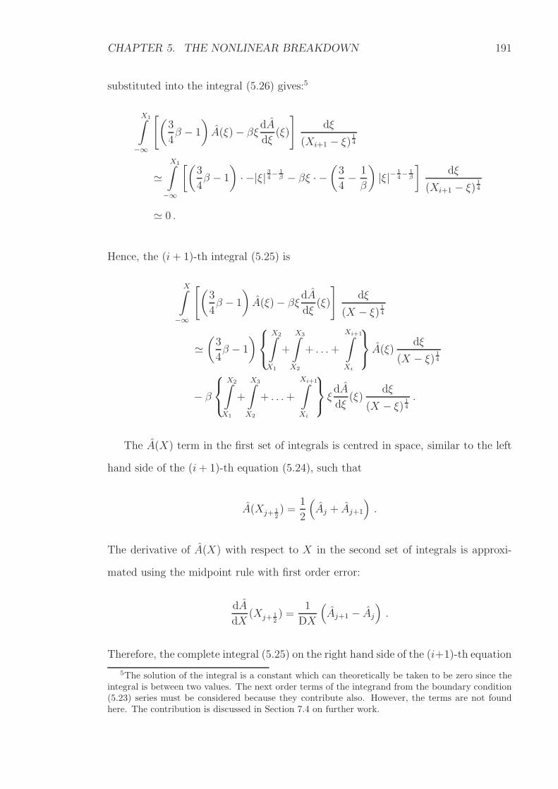
CHAPTER 5. THE NONLINEAR BREAKDOWN 191
substituted into the integral (5.26) gives:5
X1∫
−∞
[
(
3
4β − 1
)
A(ξ)− βξdAdξ
(ξ)
]
dξ
(Xi+1 − ξ)14
≃X1∫
−∞
[(
3
4β − 1
)
· −|ξ| 34− 1β − βξ · −
(
3
4− 1
β
)
|ξ|− 14− 1
β
]
dξ
(Xi+1 − ξ)14
≃ 0 .
Hence, the (i+ 1)-th integral (5.25) is
X∫
−∞
[
(
3
4β − 1
)
A(ξ)− βξdAdξ
(ξ)
]
dξ
(X − ξ) 14
≃(
3
4β − 1
)
X2∫
X1
+
X3∫
X2
+ . . .+
Xi+1∫
Xi
A(ξ)dξ
(X − ξ) 14
− β
X2∫
X1
+
X3∫
X2
+ . . .+
Xi+1∫
Xi
ξdA
dξ(ξ)
dξ
(X − ξ) 14
.
The A(X) term in the first set of integrals is centred in space, similar to the left
hand side of the (i+ 1)-th equation (5.24), such that
A(Xj+ 12) =
1
2
(
Aj + Aj+1
)
.
The derivative of A(X) with respect to X in the second set of integrals is approxi-
mated using the midpoint rule with first order error:
dA
dX(Xj+ 1
2) =
1
DX
(
Aj+1 − Aj
)
.
Therefore, the complete integral (5.25) on the right hand side of the (i+1)-th equation
5The solution of the integral is a constant which can theoretically be taken to be zero since theintegral is between two values. The next order terms of the integrand from the boundary condition(5.23) series must be considered because they contribute also. However, the terms are not foundhere. The contribution is discussed in Section 7.4 on further work.
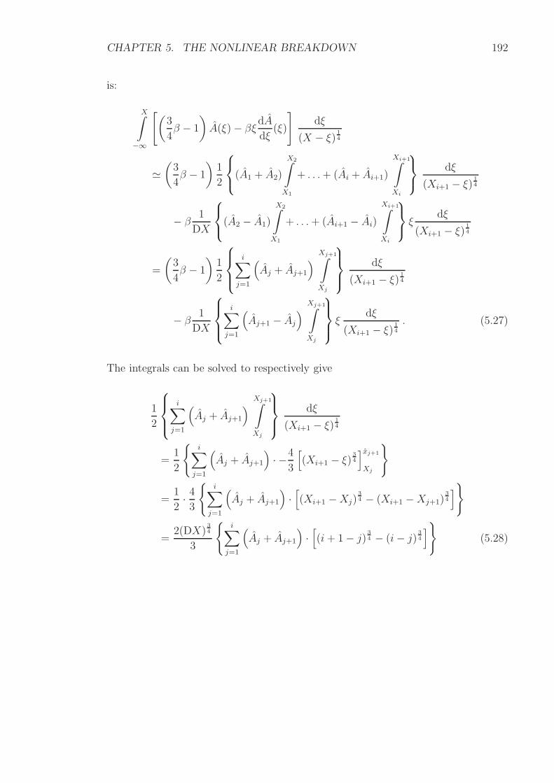
CHAPTER 5. THE NONLINEAR BREAKDOWN 192
is:
X∫
−∞
[
(
3
4β − 1
)
A(ξ)− βξdAdξ
(ξ)
]
dξ
(X − ξ) 14
≃(
3
4β − 1
)
1
2
(A1 + A2)
X2∫
X1
+ . . .+ (Ai + Ai+1)
Xi+1∫
Xi
dξ
(Xi+1 − ξ)14
− β 1
DX
(A2 − A1)
X2∫
X1
+ . . .+ (Ai+1 − Ai)
Xi+1∫
Xi
ξdξ
(Xi+1 − ξ)14
=
(
3
4β − 1
)
1
2
i∑
j=1
(
Aj + Aj+1
)
Xj+1∫
Xj
dξ
(Xi+1 − ξ)14
− β 1
DX
i∑
j=1
(
Aj+1 − Aj
)
Xj+1∫
Xj
ξdξ
(Xi+1 − ξ)14
. (5.27)
The integrals can be solved to respectively give
1
2
i∑
j=1
(
Aj + Aj+1
)
Xj+1∫
Xj
dξ
(Xi+1 − ξ)14
=1
2
i∑
j=1
(
Aj + Aj+1
)
· −43
[
(Xi+1 − ξ)34
]xj+1
Xj
=1
2· 43
i∑
j=1
(
Aj + Aj+1
)
·[
(Xi+1 −Xj)34 − (Xi+1 −Xj+1)
34
]
=2(DX)
34
3
i∑
j=1
(
Aj + Aj+1
)
·[
(i+ 1− j) 34 − (i− j) 3
4
]
(5.28)
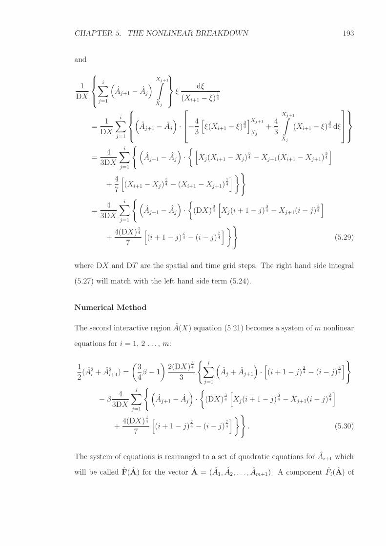
CHAPTER 5. THE NONLINEAR BREAKDOWN 193
and
1
DX
i∑
j=1
(
Aj+1 − Aj
)
Xj+1∫
Xj
ξdξ
(Xi+1 − ξ)14
=1
DX
i∑
j=1
(
Aj+1 − Aj
)
·
−43
[
ξ(Xi+1 − ξ)34
]Xj+1
Xj
+4
3
Xj+1∫
Xj
(Xi+1 − ξ)34 dξ
=4
3DX
i∑
j=1
(
Aj+1 − Aj
)
·
[
Xj(Xi+1 −Xj)34 −Xj+1(Xi+1 −Xj+1)
34
]
+4
7
[
(Xi+1 −Xj)74 − (Xi+1 −Xj+1)
74
]
=4
3DX
i∑
j=1
(
Aj+1 − Aj
)
·
(DX)34
[
Xj(i+ 1− j) 34 −Xj+1(i− j)
34
]
+4(DX)
74
7
[
(i+ 1− j) 74 − (i− j) 7
4
]
(5.29)
where DX and DT are the spatial and time grid steps. The right hand side integral
(5.27) will match with the left hand side term (5.24).
Numerical Method
The second interactive region A(X) equation (5.21) becomes a system of m nonlinear
equations for i = 1, 2 . . . , m:
1
2(A2
i + A2i+1) =
(
3
4β − 1
)
2(DX)34
3
i∑
j=1
(
Aj + Aj+1
)
·[
(i+ 1− j) 34 − (i− j) 3
4
]
− β 4
3DX
i∑
j=1
(
Aj+1 − Aj
)
·
(DX)34
[
Xj(i+ 1− j) 34 −Xj+1(i− j)
34
]
+4(DX)
74
7
[
(i+ 1− j) 74 − (i− j) 7
4
]
. (5.30)
The system of equations is rearranged to a set of quadratic equations for Ai+1 which
will be called F(A) for the vector A = (A1, A2, . . . , Am+1). A component Fi(A) of
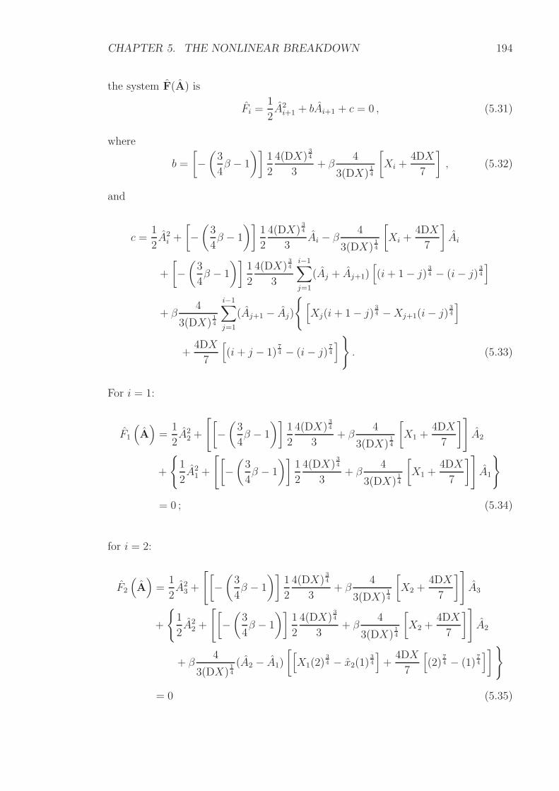
CHAPTER 5. THE NONLINEAR BREAKDOWN 194
the system F(A) is
Fi =1
2A2
i+1 + bAi+1 + c = 0 , (5.31)
where
b =
[
−(
3
4β − 1
)]
1
2
4(DX)34
3+ β
4
3(DX)14
[
Xi +4DX
7
]
, (5.32)
and
c =1
2A2
i +
[
−(
3
4β − 1
)]
1
2
4(DX)34
3Ai − β
4
3(DX)14
[
Xi +4DX
7
]
Ai
+
[
−(
3
4β − 1
)]
1
2
4(DX)34
3
i−1∑
j=1
(Aj + Aj+1)[
(i+ 1− j) 34 − (i− j) 3
4
]
+ β4
3(DX)14
i−1∑
j=1
(Aj+1 − Aj)
[
Xj(i+ 1− j) 34 −Xj+1(i− j)
34
]
+4DX
7
[
(i+ j − 1)74 − (i− j) 7
4
]
. (5.33)
For i = 1:
F1
(
A)
=1
2A2
2 +
[
[
−(
3
4β − 1
)]
1
2
4(DX)34
3+ β
4
3(DX)14
[
X1 +4DX
7
]
]
A2
+
1
2A2
1 +
[
[
−(
3
4β − 1
)]
1
2
4(DX)34
3+ β
4
3(DX)14
[
X1 +4DX
7
]
]
A1
= 0 ; (5.34)
for i = 2:
F2
(
A)
=1
2A2
3 +
[
[
−(
3
4β − 1
)]
1
2
4(DX)34
3+ β
4
3(DX)14
[
X2 +4DX
7
]
]
A3
+
1
2A2
2 +
[
[
−(
3
4β − 1
)]
1
2
4(DX)34
3+ β
4
3(DX)14
[
X2 +4DX
7
]
]
A2
+ β4
3(DX)14
(A2 − A1)
[
[
X1(2)34 − x2(1)
34
]
+4DX
7
[
(2)74 − (1)
74
]
]
= 0 (5.35)
CHAPTER 5. THE NONLINEAR BREAKDOWN 195
and so forth.
5.2.1 The Minimising Function Φ , Eigenvalue β & Boundary
Value Constant λ2
The boundary condition (5.23) at the start of the computational domain X = X1 is
A1 = −|X1|34− 1
β . However, the value of Am+1 at the end of the domain:
Am+1 = λ2X34− 1
β
m+1 (5.36)
remains unknown since λ2 is an arbitrary constant. The boundary condition at X =
Xm+1 can be satisfactorily achieved, with the constant λ2 found, by implementation
of a minimising function. The A(X) solution must satisfy the minimising function
to be a true solution.
Treating the boundary condition (5.36) as a function of X and differentiating,
then:
dA
dX
∣
∣
∣
∣
∣
X=Xm
= A′m = λ2
(
3
4− 1
β
)
X34− 1
β−1
m .
A minimising function Φ (which is not to be confused with the Fourier transformation
in Section 3.3.3) can then be defined from the boundary condition derivative A′m:
Φ(β;Xm; Am, Am+1) =A′
m
12(Am + Am+1)
−(
3
4− 1
β
)
1
Xm
= 0 .
The minimising function is also centred in space atXm+ 12. A first order approximation
of the A′(X) term is
dA
dX
∣
∣
∣
∣
∣
X=Xm
=Am+1 − Am
DX.
A second order approximation to A′(X) is not appropriate since there is a discon-
tinuity along the X-axis according to the analysis in Section 5.2.3. Therefore, the
CHAPTER 5. THE NONLINEAR BREAKDOWN 196
minimising function Φ is
Φ(β;Xm; Am, Am+1) =Am+1 − Am
DX · 12(Am + Am+1)
−(
3
4− 1
β
)
1
Xm
= 0 (5.37)
and the value of the true eigenvalue β is found from rearranging (5.37):
β =
∣
∣
∣
∣
∣
Xm ·(
Am+1 − Am
DX · 12(Am + Am+1)
)
− 3
4
∣
∣
∣
∣
∣
−1
. (5.38)
The minimising function Φ is so-called because it is used to force the iterate
solution towards the boundary condition at X = Xm+1, and thus the true A(X)
solution, with each iteration of Newton’s method. The minimising function is also
used to help determine the true A(X) solution and a narrow neighbourhood of the
true eigenvalue β when using the shooting method.
Furthermore, the value of constant λ2 is found from rearranging the boundary
condition (5.36) at X = Xm+1 :
λ2 =Am+1
X34− 1
β
m+1
(5.39)
using the values for (5.37).
The use of (5.37), (5.38) and (5.39) in situ is shown in Sections 5.2.2 and 5.2.4.
5.2.2 Numerical Shooting Method
The eigenvalue β is known to be in the range 0 < β < 43in order for first interactive
stage A(x, T ) to be large at breakdown and second interactive stage A(X) to be of
order unity. The range of eigenvalue is discretised by uniform increments of ∆β =
0.01, starting at β1 = 0.01 and ending at β133 = 1.33, such that βk = β1 + (k− 1)∆β
for k = 1, 2, . . . , 1.33.
A crude technique is to start at β1 = 0.01 and shoot from the known boundary
condition A1 (5.23) to solve each Ai+1 of the component equation (5.31) in turn
for i = 1, 2, . . . , m. Next, march forward in β by the increment of ∆β = 0.01 to
CHAPTER 5. THE NONLINEAR BREAKDOWN 197
β2 = 0.02 and repeat the shooting, until β = 1.33 is reached.
The Ai+1 solution to each component equation:
Fi =1
2A2
i+1 + bAi+1 + c = 0
is given by the quadratic formula:
Ai+1 =−b±
√b2 − 4ac
2a
where from the numerical treatment in Section 5.2: a = 12and b, c are given by
(5.32), (5.33) respectively. A choice of sign must be made for the solution Ai+1 of the
quadratic formula. The solution is expected to be discontinuous at X = 0, negative
for X < 0 and positive for X > 0 from the work by Smith & Elliott (1985) and the
discontinuous functions analysis in Section 5.2.3. Hence, the corresponding root is
chosen. For i = 1, the A2 solution to the F1(A) equation (5.34) is:
A2 = −[
[
−(
3
4β − 1
)]
1
2
4(DX)34
3+ β
4
3(DX)14
[
X1 +4DX
7
]
]
−[
[
−(
3
4β − 1
)]
1
2
4(DX)34
3+ β
4
3(DX)14
[
X1 +4DX
7
]
]2
− 2
1
2A2
1 +
[
[
−(
3
4β − 1
)]
1
2
4(DX)34
3+ β
4
3(DX)14
[
X1 +4DX
7
]
]
A1
with the negative root chosen because X2 < 0.
Better approximations to the solution and hence the eigenvalue are made by
repeating the same crude technique for a narrower range of β. If at some βk: Φ < 0
and at the adjacent increment βk+∆β: Φ > 0 (or vice versa, βk: Φ > 0 and βk+∆β:
Φ < 0) then by the intermediate value theorem, Φ = 0 at some value of β in the
range (βk, βk + ∆β). The process of discretisation and shooting is repeated for the
range until the true eigenvalue is found to, for example, 3 significant figures.
The true A(X) solution, corresponding with the true eigenvalue β, occurs when
CHAPTER 5. THE NONLINEAR BREAKDOWN 198
the minimising function Φ (5.37) is satisfied. When the true solution is found then
the constant λ2 is given by (5.39).
The shooting method is tested in Section 5.3.1.
5.2.3 Discontinuous A(x, T ) & A(X) Analysis
The A(x, T ) solvability condition (4.1):
A2(x, T )− x2 + 2a(T ) = − 234
Γ(54)
x∫
−∞
∂A
∂T(ξ, T )
dξ
(x− ξ) 14
,
of which the second interactive stage A(X) equation (5.21):
A2(X) = − 234
Γ(54)
X∫
−∞
[
−(
3
4β − 1
)
A(ξ) + βξdA
dξ(ξ)
]
dξ
(X − ξ) 14
originates, can be shown to admit discontinuous forms of A(x, T ) like travelling Heav-
iside function waves (although they are not solved with boundary conditions). If dis-
continuous forms of A(x, T ) can exist for the solvability condition then by the series
expansion (5.6):
A(x, T ) = (Ts − T )34n−1A(X) + . . . A(X) = O(1) ,
discontinuous forms of A(X) can also exist in the second interactive region.
When A(x, T ) becomes large and negative, and the term −x + 2a(T ) becomes
insignificant, then the Abel inverse transform version of the A(x, T ) equation, that is
(3.49) without bar or subscript notation, becomes:
∂A
∂T(x, T ) = −Γ(
54)
254π
∂
∂x
x∫
−∞
A2(ξ, T )dξ
(x− ξ) 34
. (5.40)
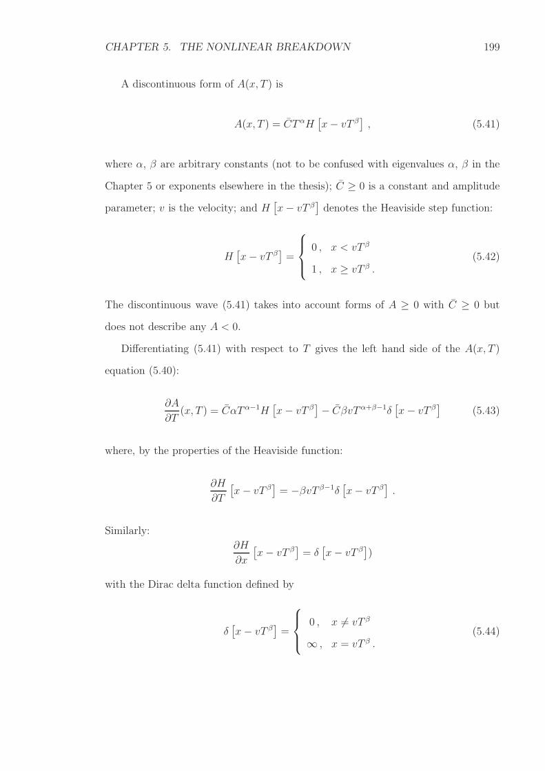
CHAPTER 5. THE NONLINEAR BREAKDOWN 199
A discontinuous form of A(x, T ) is
A(x, T ) = CT αH[
x− vT β]
, (5.41)
where α, β are arbitrary constants (not to be confused with eigenvalues α, β in the
Chapter 5 or exponents elsewhere in the thesis); C ≥ 0 is a constant and amplitude
parameter; v is the velocity; and H[
x− vT β]
denotes the Heaviside step function:
H[
x− vT β]
=
0 , x < vT β
1 , x ≥ vT β .(5.42)
The discontinuous wave (5.41) takes into account forms of A ≥ 0 with C ≥ 0 but
does not describe any A < 0.
Differentiating (5.41) with respect to T gives the left hand side of the A(x, T )
equation (5.40):
∂A
∂T(x, T ) = CαT α−1H
[
x− vT β]
− CβvT α+β−1δ[
x− vT β]
(5.43)
where, by the properties of the Heaviside function:
∂H
∂T
[
x− vT β]
= −βvT β−1δ[
x− vT β]
.
Similarly:
∂H
∂x
[
x− vT β]
= δ[
x− vT β]
)
with the Dirac delta function defined by
δ[
x− vT β]
=
0 , x 6= vT β
∞ , x = vT β .(5.44)
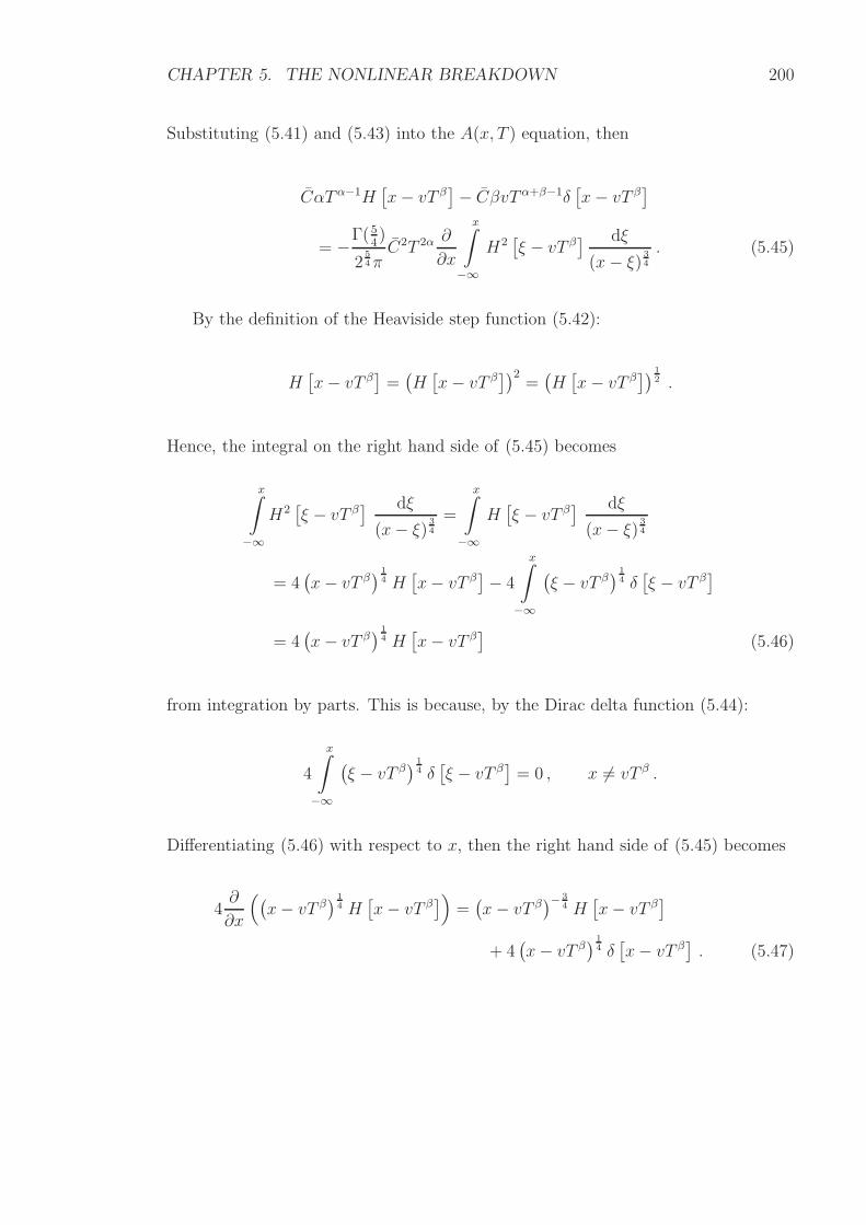
CHAPTER 5. THE NONLINEAR BREAKDOWN 200
Substituting (5.41) and (5.43) into the A(x, T ) equation, then
CαT α−1H[
x− vT β]
− CβvT α+β−1δ[
x− vT β]
= −Γ(54)
254π
C2T 2α ∂
∂x
x∫
−∞
H2[
ξ − vT β] dξ
(x− ξ) 34
. (5.45)
By the definition of the Heaviside step function (5.42):
H[
x− vT β]
=(
H[
x− vT β])2
=(
H[
x− vT β])
12 .
Hence, the integral on the right hand side of (5.45) becomes
x∫
−∞
H2[
ξ − vT β] dξ
(x− ξ) 34
=
x∫
−∞
H[
ξ − vT β] dξ
(x− ξ) 34
= 4(
x− vT β)
14 H
[
x− vT β]
− 4
x∫
−∞
(
ξ − vT β)
14 δ[
ξ − vT β]
= 4(
x− vT β)
14 H
[
x− vT β]
(5.46)
from integration by parts. This is because, by the Dirac delta function (5.44):
4
x∫
−∞
(
ξ − vT β)
14 δ[
ξ − vT β]
= 0 , x 6= vT β .
Differentiating (5.46) with respect to x, then the right hand side of (5.45) becomes
4∂
∂x
(
(
x− vT β)
14 H
[
x− vT β]
)
=(
x− vT β)− 3
4 H[
x− vT β]
+ 4(
x− vT β)
14 δ[
x− vT β]
. (5.47)
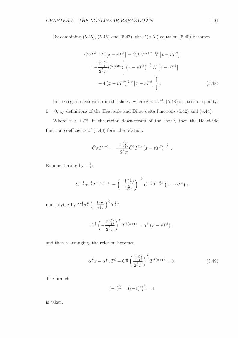
CHAPTER 5. THE NONLINEAR BREAKDOWN 201
By combining (5.45), (5.46) and (5.47), the A(x, T ) equation (5.40) becomes
CαT α−1H[
x− vT β]
− CβvT α+β−1δ[
x− vT β]
= −Γ(54)
254π
C2T 2α
(
x− vT β)− 3
4 H[
x− vT β]
+ 4(
x− vT β)
14 δ[
x− vT β]
. (5.48)
In the region upstream from the shock, where x < vT β, (5.48) is a trivial equality:
0 = 0, by definitions of the Heaviside and Dirac delta functions (5.42) and (5.44).
Where x > vT β, in the region downstream of the shock, then the Heaviside
function coefficients of (5.48) form the relation:
CαT α−1 = −Γ(54)
254π
C2T 2α(
x− vT β)− 3
4 .
Exponentiating by −43:
C− 43α− 4
3T− 43(α−1) =
(
−Γ(54)
254π
)− 43
C− 83T− 8
3α(
x− vT β)
;
multiplying by C83α
43
(
−Γ( 54)
254 π
)43
T83α:
C43
(
−Γ(54)
254π
)
43
T43(α+1) = α
43
(
x− vT β)
;
and then rearranging, the relation becomes
α43x− α 4
3 vT β − C 43
(
Γ(54)
254π
)
43
T43(α+1) = 0 . (5.49)
The branch
(−1) 43 =
(
(−1)4)
13 = 1
is taken.
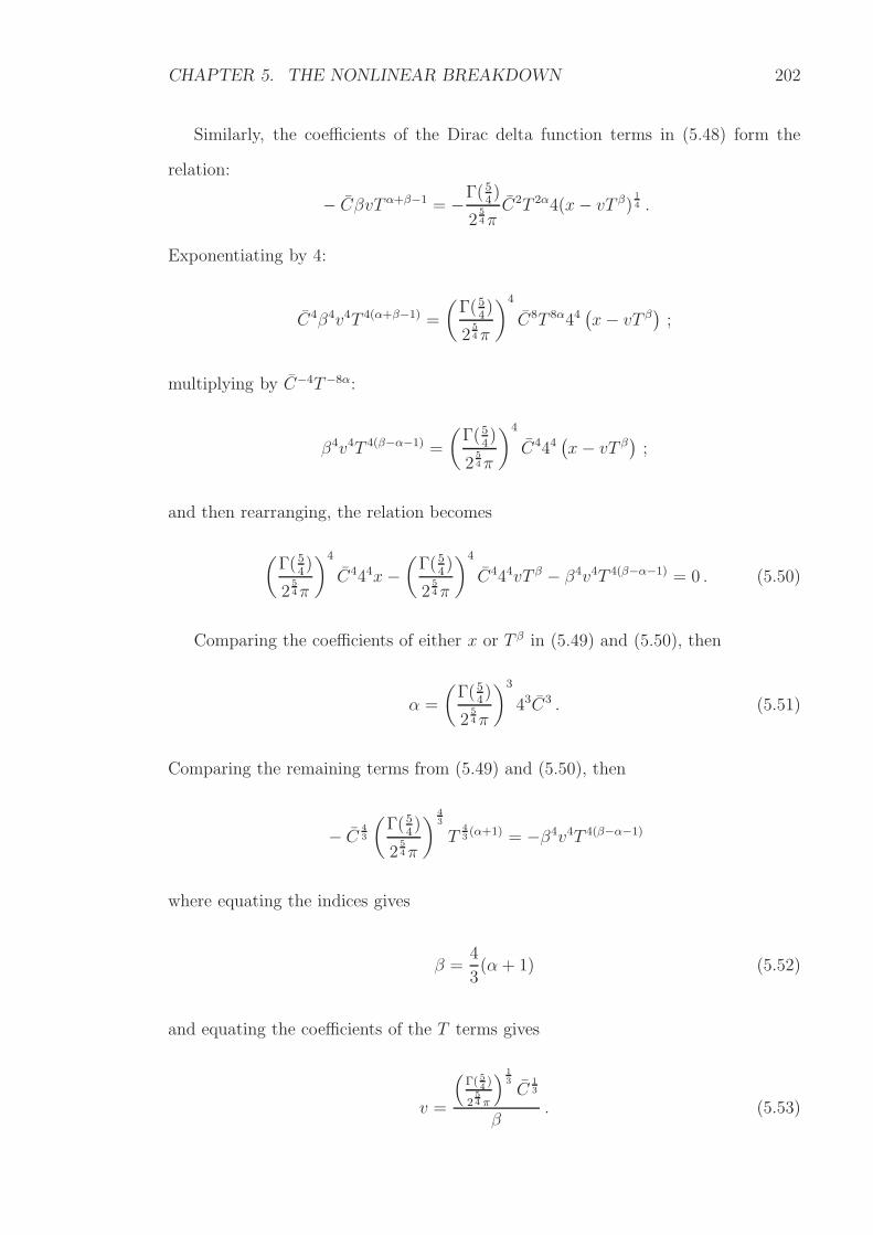
CHAPTER 5. THE NONLINEAR BREAKDOWN 202
Similarly, the coefficients of the Dirac delta function terms in (5.48) form the
relation:
− CβvT α+β−1 = −Γ(54)
254π
C2T 2α4(x− vT β)14 .
Exponentiating by 4:
C4β4v4T 4(α+β−1) =
(
Γ(54)
254π
)4
C8T 8α44(
x− vT β)
;
multiplying by C−4T−8α:
β4v4T 4(β−α−1) =
(
Γ(54)
254π
)4
C444(
x− vT β)
;
and then rearranging, the relation becomes
(
Γ(54)
254π
)4
C444x−(
Γ(54)
254π
)4
C444vT β − β4v4T 4(β−α−1) = 0 . (5.50)
Comparing the coefficients of either x or T β in (5.49) and (5.50), then
α =
(
Γ(54)
254π
)3
43C3 . (5.51)
Comparing the remaining terms from (5.49) and (5.50), then
− C 43
(
Γ(54)
254π
)
43
T43(α+1) = −β4v4T 4(β−α−1)
where equating the indices gives
β =4
3(α + 1) (5.52)
and equating the coefficients of the T terms gives
v =
(
Γ( 54)
254 π
)13
C13
β. (5.53)
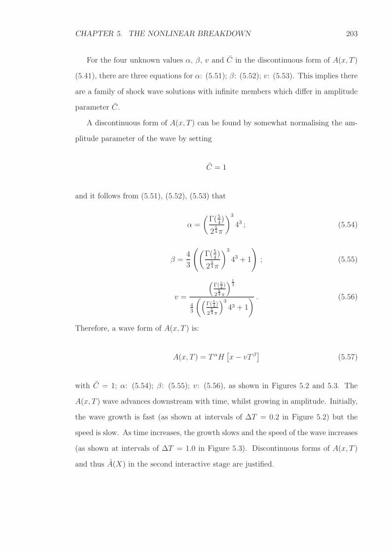
CHAPTER 5. THE NONLINEAR BREAKDOWN 203
For the four unknown values α, β, v and C in the discontinuous form of A(x, T )
(5.41), there are three equations for α: (5.51); β: (5.52); v: (5.53). This implies there
are a family of shock wave solutions with infinite members which differ in amplitude
parameter C.
A discontinuous form of A(x, T ) can be found by somewhat normalising the am-
plitude parameter of the wave by setting
C = 1
and it follows from (5.51), (5.52), (5.53) that
α =
(
Γ(54)
254π
)3
43 ; (5.54)
β =4
3
(
(
Γ(54)
254π
)3
43 + 1
)
; (5.55)
v =
(
Γ( 54)
254 π
)13
43
(
(
Γ( 54)
254 π
)3
43 + 1
) . (5.56)
Therefore, a wave form of A(x, T ) is:
A(x, T ) = T αH[
x− vT β]
(5.57)
with C = 1; α: (5.54); β: (5.55); v: (5.56), as shown in Figures 5.2 and 5.3. The
A(x, T ) wave advances downstream with time, whilst growing in amplitude. Initially,
the wave growth is fast (as shown at intervals of ∆T = 0.2 in Figure 5.2) but the
speed is slow. As time increases, the growth slows and the speed of the wave increases
(as shown at intervals of ∆T = 1.0 in Figure 5.3). Discontinuous forms of A(x, T )
and thus A(X) in the second interactive stage are justified.
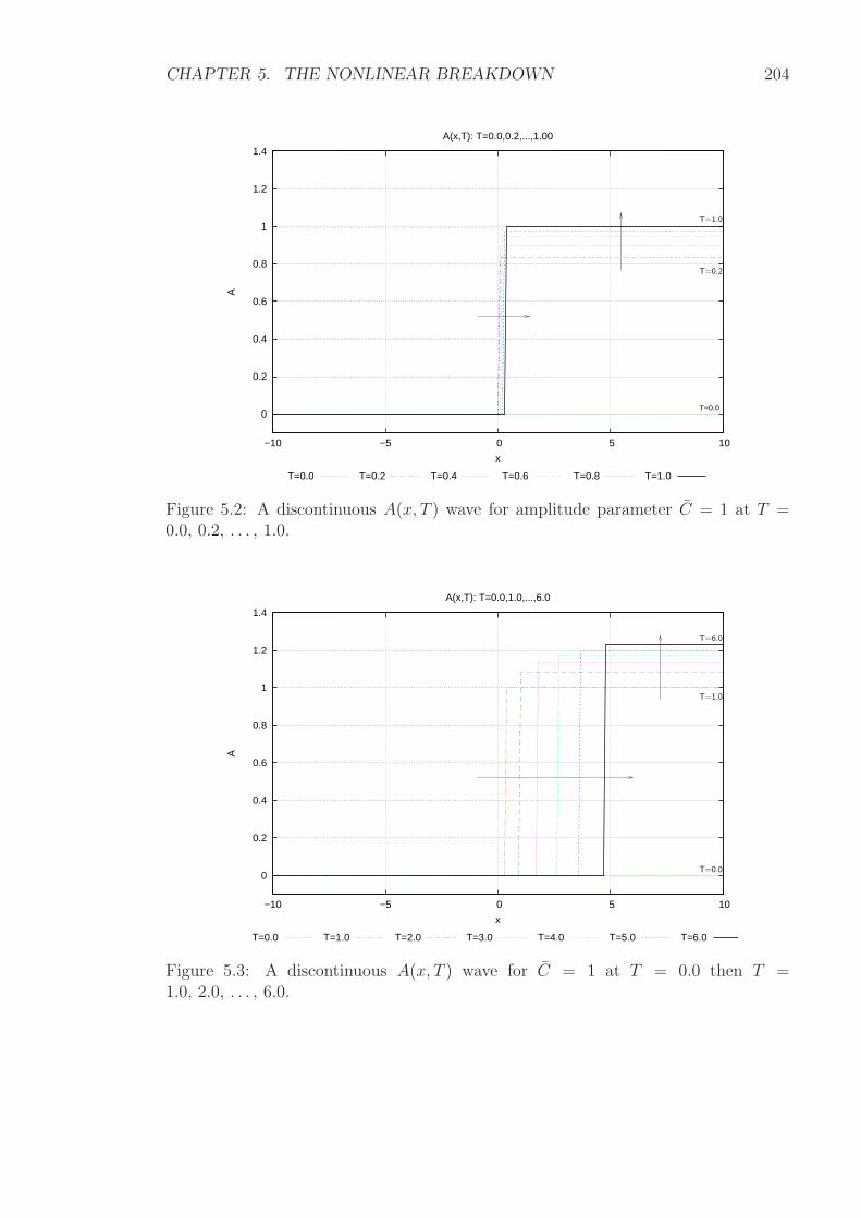
CHAPTER 5. THE NONLINEAR BREAKDOWN 204
0
0.2
0.4
0.6
0.8
1
1.2
1.4
−10 −5 0 5 10
A
x
A(x,T): T=0.0,0.2,...,1.00
T=0.0 T=0.2 T=0.4 T=0.6 T=0.8 T=1.0
T=0.0
T=0.2
T=1.0
Figure 5.2: A discontinuous A(x, T ) wave for amplitude parameter C = 1 at T =0.0, 0.2, . . . , 1.0.
0
0.2
0.4
0.6
0.8
1
1.2
1.4
−10 −5 0 5 10
A
x
A(x,T): T=0.0,1.0,...,6.0
T=0.0 T=1.0 T=2.0 T=3.0 T=4.0 T=5.0 T=6.0
T=0.0
T=1.0
T=6.0
Figure 5.3: A discontinuous A(x, T ) wave for C = 1 at T = 0.0 then T =1.0, 2.0, . . . , 6.0.
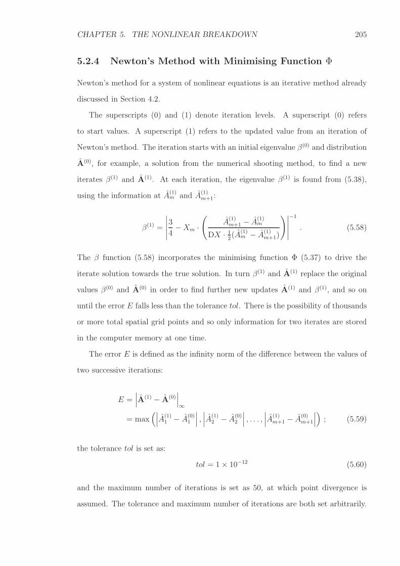
CHAPTER 5. THE NONLINEAR BREAKDOWN 205
5.2.4 Newton’s Method with Minimising Function Φ
Newton’s method for a system of nonlinear equations is an iterative method already
discussed in Section 4.2.
The superscripts (0) and (1) denote iteration levels. A superscript (0) refers
to start values. A superscript (1) refers to the updated value from an iteration of
Newton’s method. The iteration starts with an initial eigenvalue β(0) and distribution
A(0), for example, a solution from the numerical shooting method, to find a new
iterates β(1) and A(1). At each iteration, the eigenvalue β(1) is found from (5.38),
using the information at A(1)m and A
(1)m+1:
β(1) =
∣
∣
∣
∣
∣
3
4−Xm ·
(
A(1)m+1 − A
(1)m
DX · 12(A
(1)m − A(1)
m+1)
)∣
∣
∣
∣
∣
−1
. (5.58)
The β function (5.58) incorporates the minimising function Φ (5.37) to drive the
iterate solution towards the true solution. In turn β(1) and A(1) replace the original
values β(0) and A(0) in order to find further new updates A(1) and β(1), and so on
until the error E falls less than the tolerance tol. There is the possibility of thousands
or more total spatial grid points and so only information for two iterates are stored
in the computer memory at one time.
The error E is defined as the infinity norm of the difference between the values of
two successive iterations:
E =∣
∣
∣A(1) − A(0)
∣
∣
∣
∞
= max(∣
∣
∣A
(1)1 − A
(0)1
∣
∣
∣,∣
∣
∣A
(1)2 − A
(0)2
∣
∣
∣, . . . ,
∣
∣
∣A
(1)m+1 − A
(0)m+1
∣
∣
∣
)
; (5.59)
the tolerance tol is set as:
tol = 1× 10⁻¹² (5.60)
and the maximum number of iterations is set as 50, at which point divergence is
assumed. The tolerance and maximum number of iterations are both set arbitrarily.
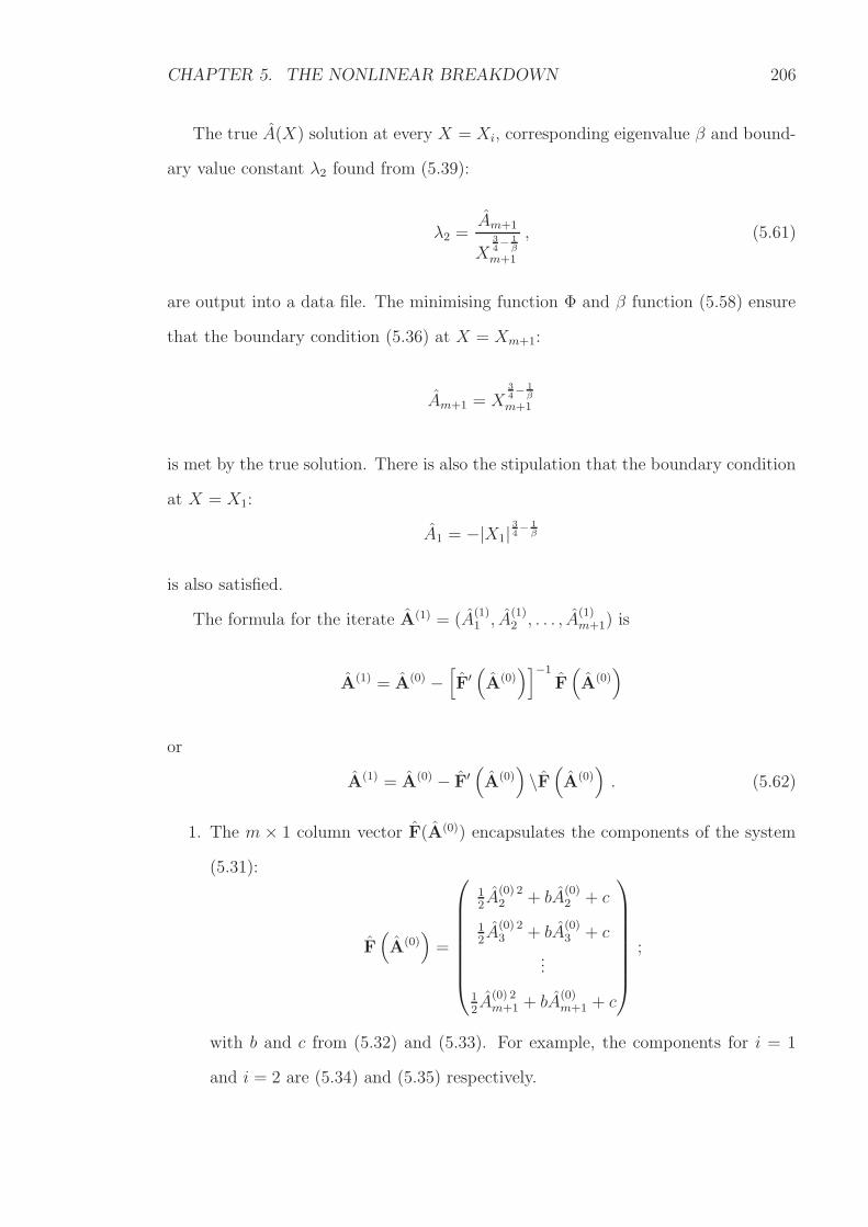
CHAPTER 5. THE NONLINEAR BREAKDOWN 206
The true A(X) solution at every X = Xi, corresponding eigenvalue β and bound-
ary value constant λ2 found from (5.39):
λ2 =Am+1
X34− 1
β
m+1
, (5.61)
are output into a data file. The minimising function Φ and β function (5.58) ensure
that the boundary condition (5.36) at X = Xm+1:
Am+1 = X34− 1
β
m+1
is met by the true solution. There is also the stipulation that the boundary condition
at X = X1:
A1 = −|X1|34− 1
β
is also satisfied.
The formula for the iterate A(1) = (A(1)1 , A
(1)2 , . . . , A
(1)m+1) is
A(1) = A(0) −[
F′(
A(0))]−1
F(
A(0))
or
A(1) = A(0) − F′(
A(0))
\F(
A(0))
. (5.62)
1. The m × 1 column vector F(A(0)) encapsulates the components of the system
(5.31):
F(
A(0))
=
12A
(0) 22 + bA
(0)2 + c
12A
(0) 23 + bA
(0)3 + c
...
12A
(0) 2m+1 + bA
(0)m+1 + c
;
with b and c from (5.32) and (5.33). For example, the components for i = 1
and i = 2 are (5.34) and (5.35) respectively.
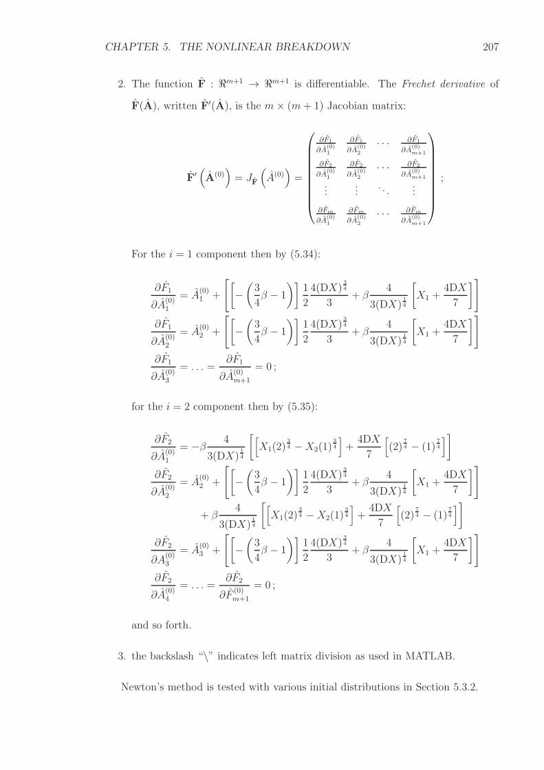
CHAPTER 5. THE NONLINEAR BREAKDOWN 207
2. The function F : ℜm+1 → ℜm+1 is differentiable. The Frechet derivative of
F(A), written F′(A), is the m× (m+ 1) Jacobian matrix:
F′(
A(0))
= JF
(
A(0))
=
∂F1
∂A(0)1
∂F1
∂A(0)2
· · · ∂F1
∂A(0)m+1
∂F2
∂A(0)1
∂F2
∂A(0)2
· · · ∂F2
∂A(0)m+1
......
. . ....
∂Fm
∂A(0)1
∂Fm
∂A(0)2
· · · ∂Fm
∂A(0)m+1
;
For the i = 1 component then by (5.34):
∂F1
∂A(0)1
= A(0)1 +
[
[
−(
3
4β − 1
)]
1
2
4(DX)34
3+ β
4
3(DX)14
[
X1 +4DX
7
]
]
∂F1
∂A(0)2
= A(0)2 +
[
[
−(
3
4β − 1
)]
1
2
4(DX)34
3+ β
4
3(DX)14
[
X1 +4DX
7
]
]
∂F1
∂A(0)3
= . . . =∂F1
∂A(0)m+1
= 0 ;
for the i = 2 component then by (5.35):
∂F2
∂A(0)1
= −β 4
3(DX)14
[
[
X1(2)34 −X2(1)
34
]
+4DX
7
[
(2)74 − (1)
74
]
]
∂F2
∂A(0)2
= A(0)2 +
[
[
−(
3
4β − 1
)]
1
2
4(DX)34
3+ β
4
3(DX)14
[
X1 +4DX
7
]
]
+ β4
3(DX)14
[
[
X1(2)34 −X2(1)
34
]
+4DX
7
[
(2)74 − (1)
74
]
]
∂F2
∂A(0)3
= A(0)3 +
[
[
−(
3
4β − 1
)]
1
2
4(DX)34
3+ β
4
3(DX)14
[
X1 +4DX
7
]
]
∂F2
∂A(0)4
= . . . =∂F2
∂F(0)m+1
= 0 ;
and so forth.
3. the backslash “\” indicates left matrix division as used in MATLAB.
Newton’s method is tested with various initial distributions in Section 5.3.2.
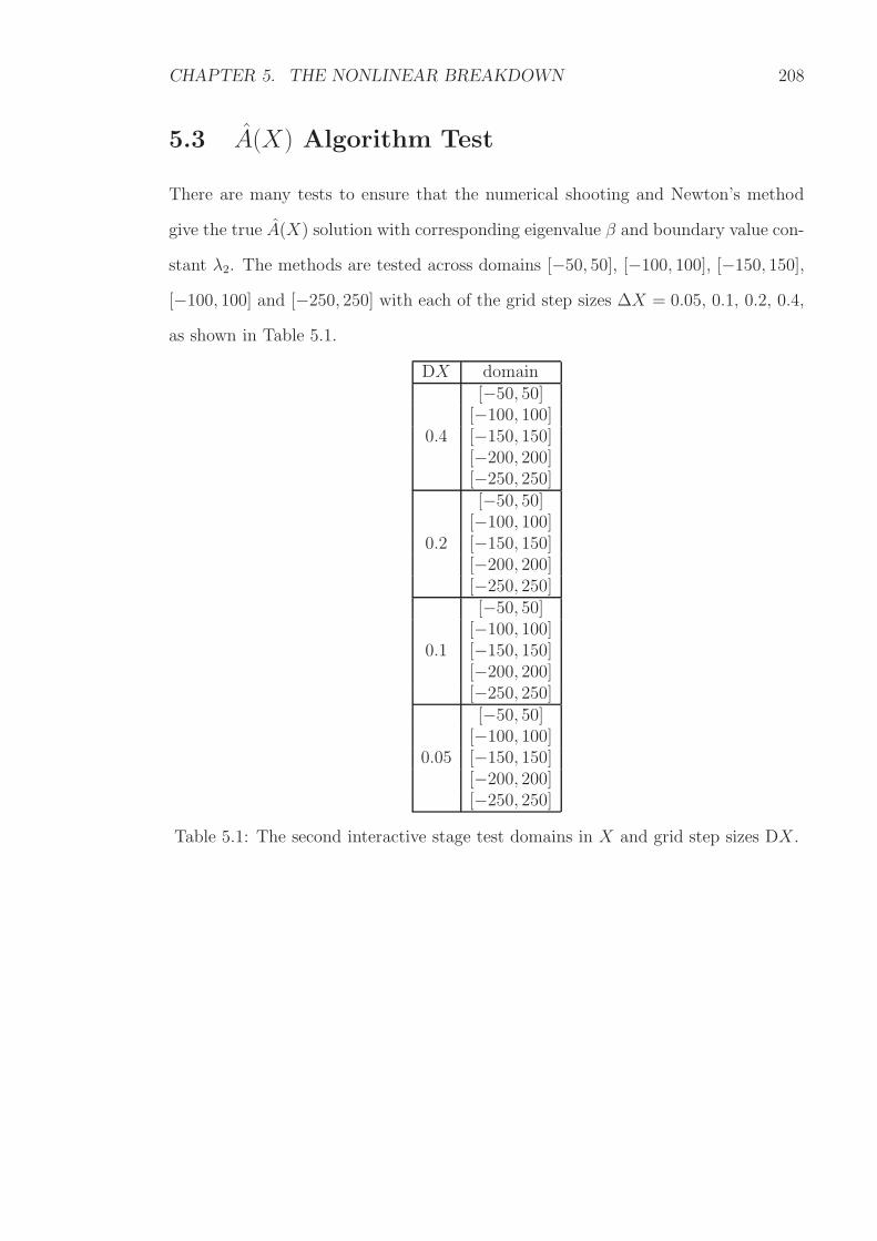
CHAPTER 5. THE NONLINEAR BREAKDOWN 208
5.3 A(X) Algorithm Test
There are many tests to ensure that the numerical shooting and Newton’s method
give the true A(X) solution with corresponding eigenvalue β and boundary value con-
stant λ2. The methods are tested across domains [−50, 50], [−100, 100], [−150, 150],
[−100, 100] and [−250, 250] with each of the grid step sizes ∆X = 0.05, 0.1, 0.2, 0.4,
as shown in Table 5.1.
DX domain
0.4
[−50, 50][−100, 100][−150, 150][−200, 200][−250, 250]
0.2
[−50, 50][−100, 100][−150, 150][−200, 200][−250, 250]
0.1
[−50, 50][−100, 100][−150, 150][−200, 200][−250, 250]
0.05
[−50, 50][−100, 100][−150, 150][−200, 200][−250, 250]
Table 5.1: The second interactive stage test domains in X and grid step sizes DX .
CHAPTER 5. THE NONLINEAR BREAKDOWN 209
5.3.1 Numerical Shooting Method Test
The numerical shooting method is working correctly if the A(X) solutions for domains
and step sizes DX from Table 5.1, corresponding eigenvalue β and boundary condition
constant λ2, converge to their true values as the size of the domain increases and the
step size decreases.
Test Results for Eigenvalue β & Boundary Value Constant λ2
The true eigenvalue β ∈(
0, 43
)
is given when the minimising function Φ = 0, as defined
by (5.37). The adopted “true” eigenvalue β and boundary condition constant λ2 are
those when Φ is closest to zero. The results for eigenvalue β and boundary condition
constant λ2 are displayed in Table 5.2. There appears to be no discernible pattern for
Φ when compared to increase in size of domain and/or decrease in step size except
that it is always small with orders of magnitude between 10−7 and 10−9.
By inspection, the eigenvalue when Φ is closest to zero is independent of domain,
particularly when the step size DX ≤ 0.2. (See Figure 5.4.) The eigenvalue is
dependent on step size, but converges to a constant value β = 1.23 (rounded up to 3
significant figures, because of Figure 5.5) as step size decreases.
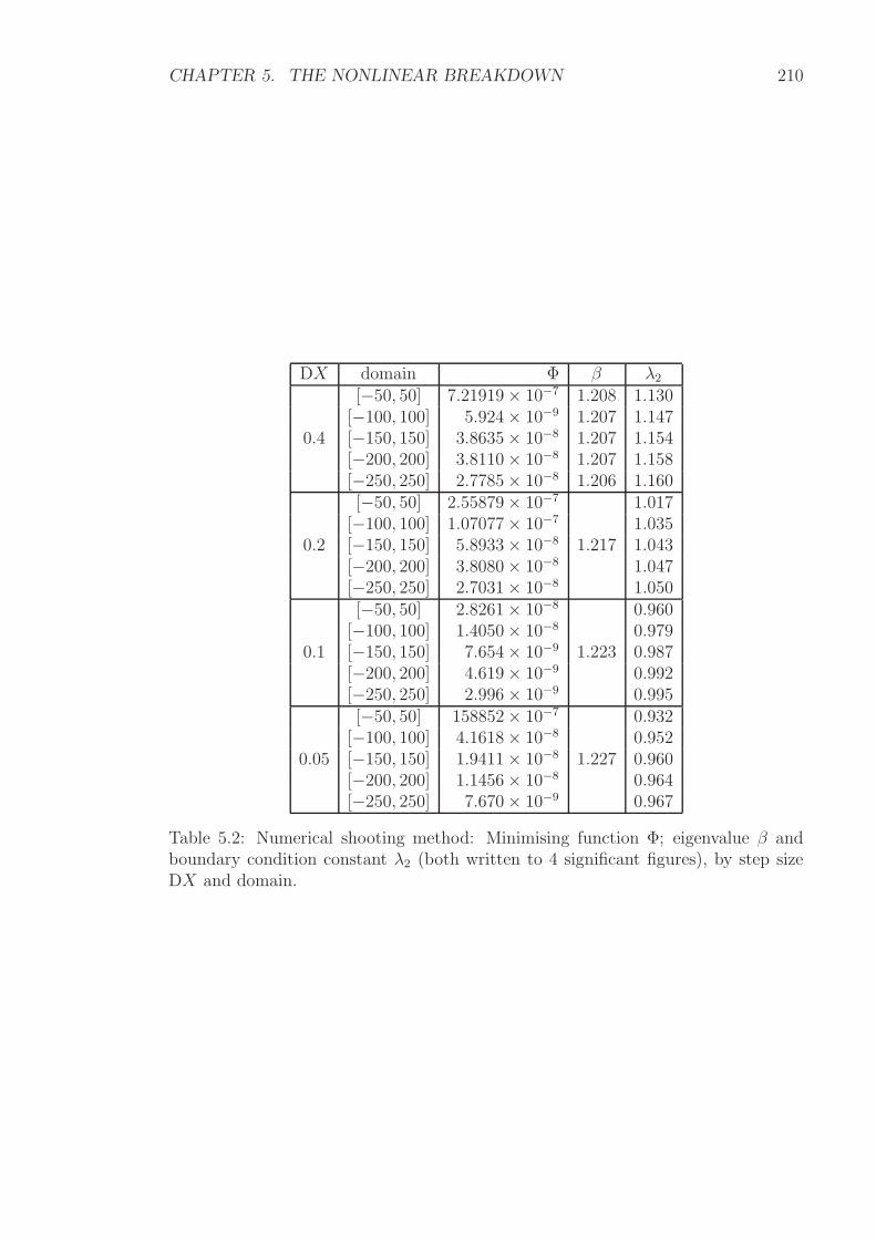
CHAPTER 5. THE NONLINEAR BREAKDOWN 210
DX domain Φ β λ2
0.4
[−50, 50] 7.21919× 10⁻⁷ 1.208 1.130[−100, 100] 5.924× 10⁻⁹ 1.207 1.147[−150, 150] 3.8635× 10⁻⁸ 1.207 1.154[−200, 200] 3.8110× 10⁻⁸ 1.207 1.158[−250, 250] 2.7785× 10⁻⁸ 1.206 1.160
0.2
[−50, 50] 2.55879× 10⁻⁷
1.217
1.017[−100, 100] 1.07077× 10⁻⁷ 1.035[−150, 150] 5.8933× 10⁻⁸ 1.043[−200, 200] 3.8080× 10⁻⁸ 1.047[−250, 250] 2.7031× 10⁻⁸ 1.050
0.1
[−50, 50] 2.8261× 10⁻⁸
1.223
0.960[−100, 100] 1.4050× 10⁻⁸ 0.979[−150, 150] 7.654× 10⁻⁹ 0.987[−200, 200] 4.619× 10⁻⁹ 0.992[−250, 250] 2.996× 10⁻⁹ 0.995
0.05
[−50, 50] 158852× 10−7
1.227
0.932[−100, 100] 4.1618× 10⁻⁸ 0.952[−150, 150] 1.9411× 10⁻⁸ 0.960[−200, 200] 1.1456× 10⁻⁸ 0.964[−250, 250] 7.670× 10⁻⁹ 0.967
Table 5.2: Numerical shooting method: Minimising function Φ; eigenvalue β andboundary condition constant λ2 (both written to 4 significant figures), by step sizeDX and domain.
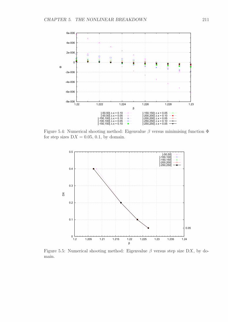
CHAPTER 5. THE NONLINEAR BREAKDOWN 211
-8e-006
-6e-006
-4e-006
-2e-006
0
2e-006
4e-006
6e-006
1.22 1.222 1.224 1.226 1.228 1.23
Φ
β
[-50,50] ∆ x = 0.10[-50,50] ∆ x = 0.05
[-100,100] ∆ x = 0.10[-100,100] ∆ x = 0.05[-150,150] ∆ x = 0.10
[-150,150] ∆ x = 0.05[-200,200] ∆ x = 0.10[-200,200] ∆ x = 0.05[-250,250] ∆ x = 0.10[-250,250] ∆ x = 0.05
Figure 5.4: Numerical shooting method: Eigenvalue β versus minimising function Φfor step sizes DX = 0.05, 0.1, by domain.
0
0.1
0.2
0.3
0.4
0.5
1.2 1.205 1.21 1.215 1.22 1.225 1.23 1.235 1.24
0.05
DX
β
[-50,50][-100,100][-150,150][-200,200][-250,250]
Figure 5.5: Numerical shooting method: Eigenvalue β versus step size DX , by do-main.
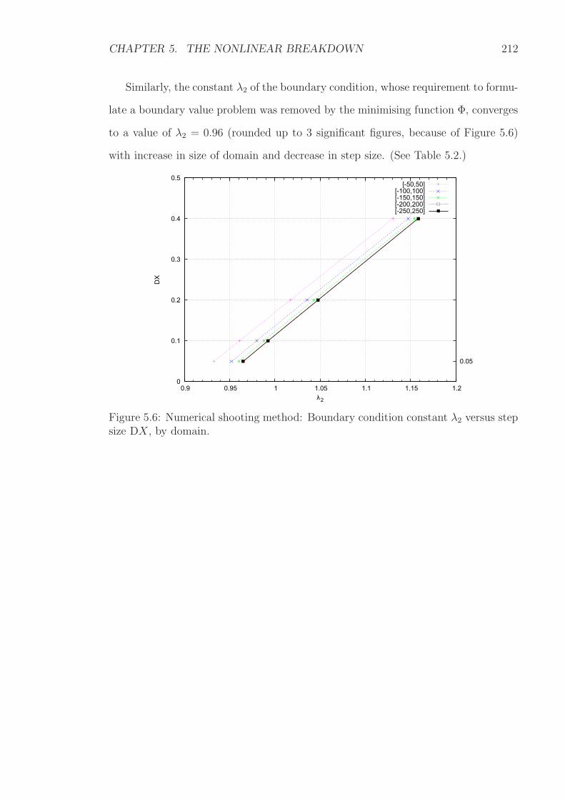
CHAPTER 5. THE NONLINEAR BREAKDOWN 212
Similarly, the constant λ2 of the boundary condition, whose requirement to formu-
late a boundary value problem was removed by the minimising function Φ, converges
to a value of λ2 = 0.96 (rounded up to 3 significant figures, because of Figure 5.6)
with increase in size of domain and decrease in step size. (See Table 5.2.)
0
0.1
0.2
0.3
0.4
0.5
0.9 0.95 1 1.05 1.1 1.15 1.2
0.05
DX
λ2
[-50,50][-100,100][-150,150][-200,200][-250,250]
Figure 5.6: Numerical shooting method: Boundary condition constant λ2 versus stepsize DX , by domain.
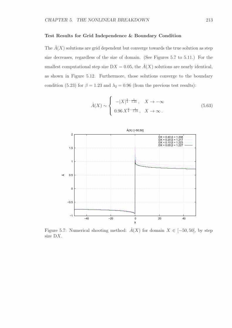
CHAPTER 5. THE NONLINEAR BREAKDOWN 213
Test Results for Grid Independence & Boundary Condition
The A(X) solutions are grid dependent but converge towards the true solution as step
size decreases, regardless of the size of domain. (See Figures 5.7 to 5.11.) For the
smallest computational step size DX = 0.05, the A(X) solutions are nearly identical,
as shown in Figure 5.12. Furthermore, those solutions converge to the boundary
condition (5.23) for β = 1.23 and λ2 = 0.96 (from the previous test results):
A(X) ∼
−|X| 34− 11.23 , X → −∞
0.96X34− 1
1.23 , X →∞ .(5.63)
−1
−0.5
0
0.5
1
1.5
2
−40 −20 0 20 40
Â
X
Â(X): [−50,50]
DX = 0.40 β = 1.208DX = 0.20 β = 1.217DX = 0.10 β = 1.223DX = 0.05 β = 1.227
Figure 5.7: Numerical shooting method: A(X) for domain X ∈ [−50, 50], by stepsize DX .
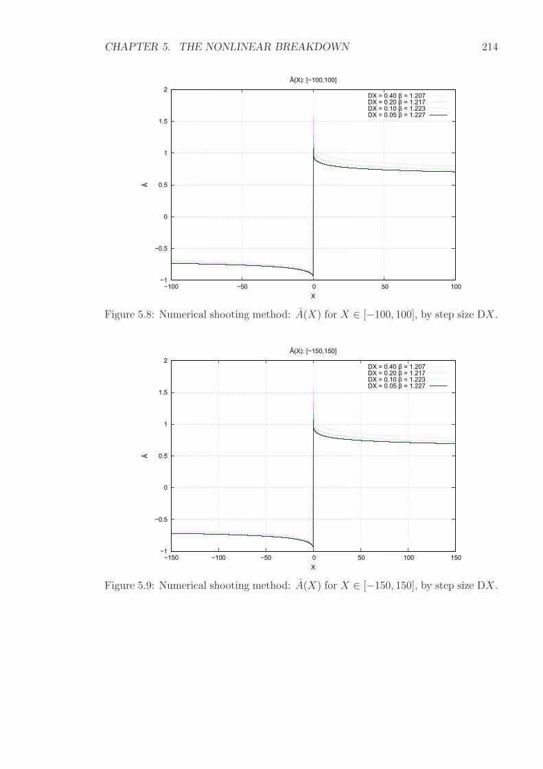
CHAPTER 5. THE NONLINEAR BREAKDOWN 214
−1
−0.5
0
0.5
1
1.5
2
−100 −50 0 50 100
Â
X
Â(X): [−100,100]
DX = 0.40 β = 1.207DX = 0.20 β = 1.217DX = 0.10 β = 1.223DX = 0.05 β = 1.227
Figure 5.8: Numerical shooting method: A(X) for X ∈ [−100, 100], by step size DX .
−1
−0.5
0
0.5
1
1.5
2
−150 −100 −50 0 50 100 150
Â
X
Â(X): [−150,150]
DX = 0.40 β = 1.207DX = 0.20 β = 1.217DX = 0.10 β = 1.223DX = 0.05 β = 1.227
Figure 5.9: Numerical shooting method: A(X) for X ∈ [−150, 150], by step size DX .
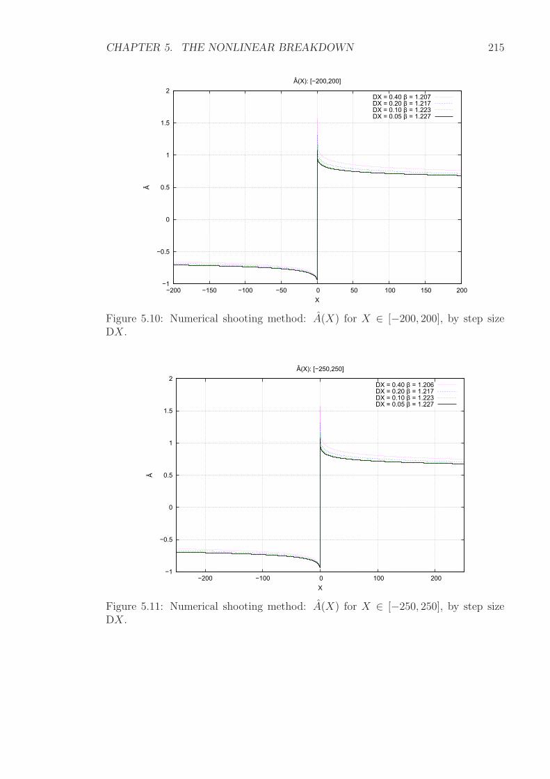
CHAPTER 5. THE NONLINEAR BREAKDOWN 215
−1
−0.5
0
0.5
1
1.5
2
−200 −150 −100 −50 0 50 100 150 200
Â
X
Â(X): [−200,200]
DX = 0.40 β = 1.207DX = 0.20 β = 1.217DX = 0.10 β = 1.223DX = 0.05 β = 1.227
Figure 5.10: Numerical shooting method: A(X) for X ∈ [−200, 200], by step sizeDX .
−1
−0.5
0
0.5
1
1.5
2
−200 −100 0 100 200
Â
X
Â(X): [−250,250]
DX = 0.40 β = 1.206DX = 0.20 β = 1.217DX = 0.10 β = 1.223DX = 0.05 β = 1.227
Figure 5.11: Numerical shooting method: A(X) for X ∈ [−250, 250], by step sizeDX .
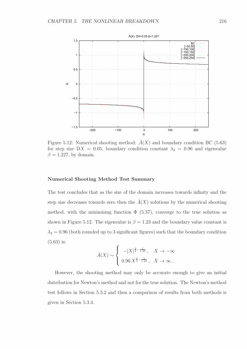
CHAPTER 5. THE NONLINEAR BREAKDOWN 216
−1.5
−1
−0.5
0
0.5
1
1.5
−200 −100 0 100 200
Â
X
Â(X): DX=0.05 β=1.227
BC[−50,50]
[−100,100][−150,150][−200,200][−250,250]
Figure 5.12: Numerical shooting method: A(X) and boundary condition BC (5.63)for step size DX = 0.05, boundary condition constant λ2 = 0.96 and eigenvalueβ = 1.227, by domain.
Numerical Shooting Method Test Summary
The test concludes that as the size of the domain increases towards infinity and the
step size decreases towards zero then the A(X) solutions by the numerical shooting
method, with the minimising function Φ (5.37), converge to the true solution as
shown in Figure 5.12. The eigenvalue is β = 1.23 and the boundary value constant is
λ2 = 0.96 (both rounded up to 3 significant figures) such that the boundary condition
(5.63) is:
A(X) ∼
−|X| 34− 11.23 , X → −∞
0.96X34− 1
1.23 , X →∞ .
However, the shooting method may only be accurate enough to give an initial
distribution for Newton’s method and not for the true solution. The Newton’s method
test follows in Section 5.3.2 and then a comparison of results from both methods is
given in Section 5.3.4.
CHAPTER 5. THE NONLINEAR BREAKDOWN 217
5.3.2 Newton’s Method Test
Newton’s method with the minimising function Φ (5.37) is tested based on the New-
ton’s method test in Section 4.4 and is deemed to be working correctly if all the
following conditions are met.
1. The error E (5.59) reduces quadratically towards zero with each iteration when
the iterate is sufficiently close to the true solution but only if there is no inter-
ference from the minimising function driving the iterate solution towards the
boundary condition at X = Xm+1 with each iteration. The initial value of
β(0) = β(1) is static with each iteration.
2. The boundary conditions (5.23):
A(X) ∼
−|X| 34− 1β , X = X1
λ2X34− 1
β , X = Xm+1
are satisfied. The constant λ2 is to be found. Moreover, the solution must
approach the boundary condition smoothly as |X| becomes large such that the
solution does not oscillate near the end points.
3. The A(X) solution converges to the true solution whilst the eigenvalue β and
boundary value constant λ2 converge to their respective true values as the size
of domain increases towards infinity and the step size DX decreases towards
zero. The test domains and step sizes are in Table 5.1.
4. The true A(X) solution, eigenvalue β and boundary value constant λ2 are
similar to their respective values from the numerical shooting method. A com-
parison of results is given in Section 5.3.4.
5.3.3 The Initial Conditions
There are three types of initial distribution A(0) and initial eigenvalue β(0) for testing
Newton’s method with the minimising function.
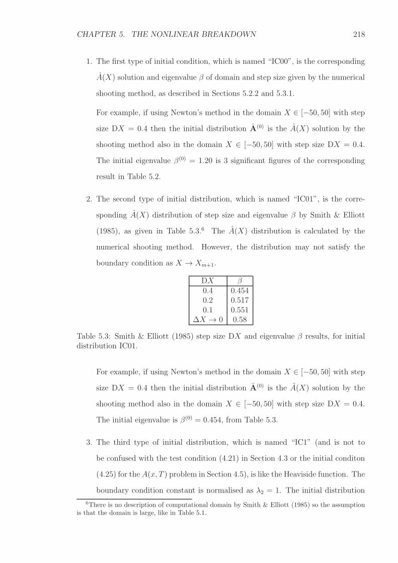
CHAPTER 5. THE NONLINEAR BREAKDOWN 218
1. The first type of initial condition, which is named “IC00”, is the corresponding
A(X) solution and eigenvalue β of domain and step size given by the numerical
shooting method, as described in Sections 5.2.2 and 5.3.1.
For example, if using Newton’s method in the domain X ∈ [−50, 50] with step
size DX = 0.4 then the initial distribution A(0) is the A(X) solution by the
shooting method also in the domain X ∈ [−50, 50] with step size DX = 0.4.
The initial eigenvalue β(0) = 1.20 is 3 significant figures of the corresponding
result in Table 5.2.
2. The second type of initial distribution, which is named “IC01”, is the corre-
sponding A(X) distribution of step size and eigenvalue β by Smith & Elliott
(1985), as given in Table 5.3.6 The A(X) distribution is calculated by the
numerical shooting method. However, the distribution may not satisfy the
boundary condition as X → Xm+1.
DX β0.4 0.4540.2 0.5170.1 0.551
∆X → 0 0.58
Table 5.3: Smith & Elliott (1985) step size DX and eigenvalue β results, for initialdistribution IC01.
For example, if using Newton’s method in the domain X ∈ [−50, 50] with step
size DX = 0.4 then the initial distribution A(0) is the A(X) solution by the
shooting method also in the domain X ∈ [−50, 50] with step size DX = 0.4.
The initial eigenvalue is β(0) = 0.454, from Table 5.3.
3. The third type of initial distribution, which is named “IC1” (and is not to
be confused with the test condition (4.21) in Section 4.3 or the initial conditon
(4.25) for theA(x, T ) problem in Section 4.5), is like the Heaviside function. The
boundary condition constant is normalised as λ2 = 1. The initial distribution
6There is no description of computational domain by Smith & Elliott (1985) so the assumptionis that the domain is large, like in Table 5.1.
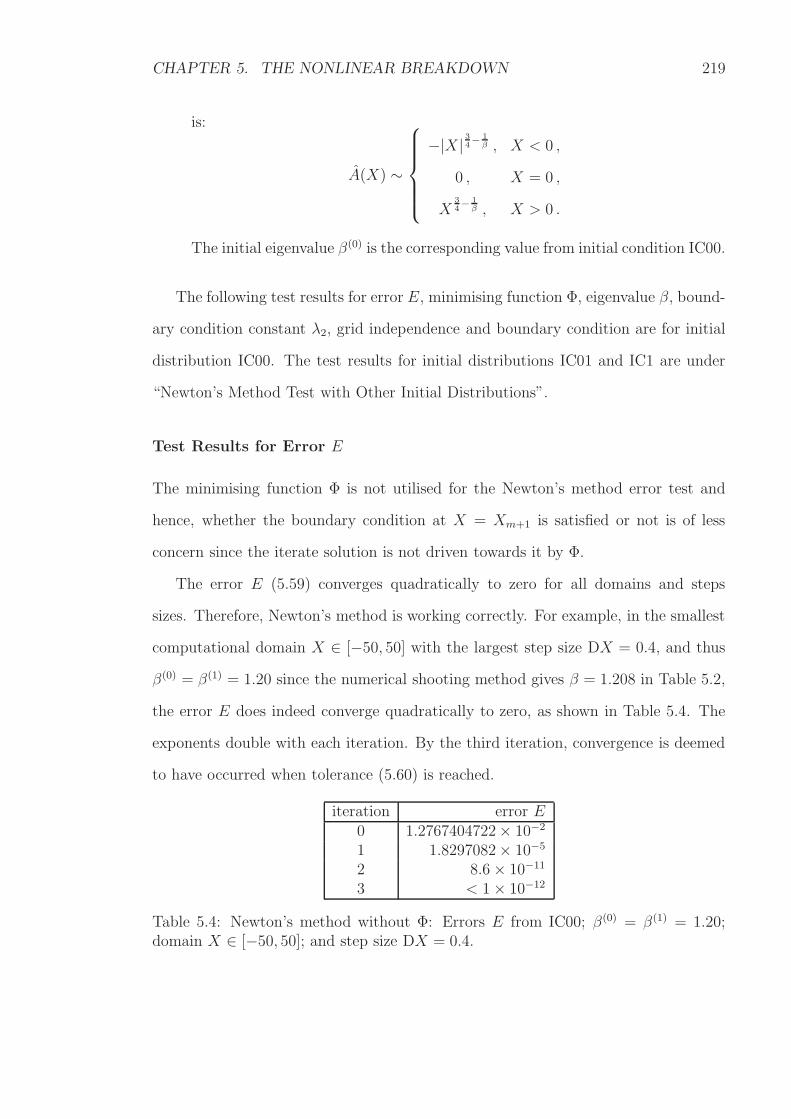
CHAPTER 5. THE NONLINEAR BREAKDOWN 219
is:
A(X) ∼
−|X| 34− 1β , X < 0 ,
0 , X = 0 ,
X34− 1
β , X > 0 .
The initial eigenvalue β(0) is the corresponding value from initial condition IC00.
The following test results for error E, minimising function Φ, eigenvalue β, bound-
ary condition constant λ2, grid independence and boundary condition are for initial
distribution IC00. The test results for initial distributions IC01 and IC1 are under
“Newton’s Method Test with Other Initial Distributions”.
Test Results for Error E
The minimising function Φ is not utilised for the Newton’s method error test and
hence, whether the boundary condition at X = Xm+1 is satisfied or not is of less
concern since the iterate solution is not driven towards it by Φ.
The error E (5.59) converges quadratically to zero for all domains and steps
sizes. Therefore, Newton’s method is working correctly. For example, in the smallest
computational domain X ∈ [−50, 50] with the largest step size DX = 0.4, and thus
β(0) = β(1) = 1.20 since the numerical shooting method gives β = 1.208 in Table 5.2,
the error E does indeed converge quadratically to zero, as shown in Table 5.4. The
exponents double with each iteration. By the third iteration, convergence is deemed
to have occurred when tolerance (5.60) is reached.
iteration error E0 1.2767404722× 10⁻²
1 1.8297082× 10⁻⁵
2 8.6× 10⁻¹¹
3 < 1× 10⁻¹²
Table 5.4: Newton’s method without Φ: Errors E from IC00; β(0) = β(1) = 1.20;domain X ∈ [−50, 50]; and step size DX = 0.4.
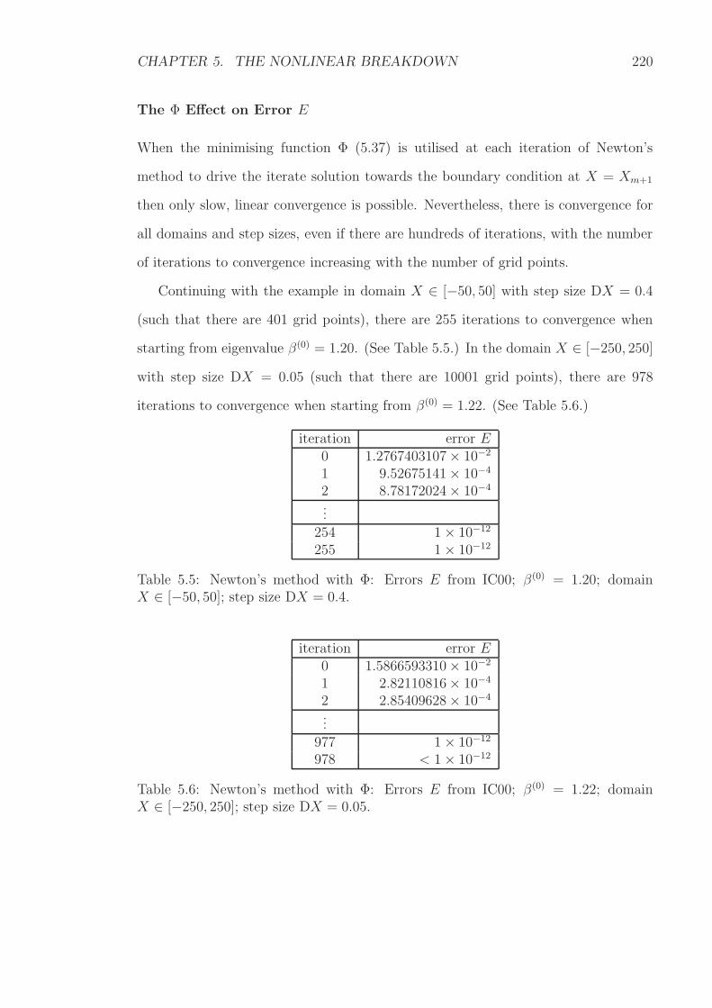
CHAPTER 5. THE NONLINEAR BREAKDOWN 220
The Φ Effect on Error E
When the minimising function Φ (5.37) is utilised at each iteration of Newton’s
method to drive the iterate solution towards the boundary condition at X = Xm+1
then only slow, linear convergence is possible. Nevertheless, there is convergence for
all domains and step sizes, even if there are hundreds of iterations, with the number
of iterations to convergence increasing with the number of grid points.
Continuing with the example in domain X ∈ [−50, 50] with step size DX = 0.4
(such that there are 401 grid points), there are 255 iterations to convergence when
starting from eigenvalue β(0) = 1.20. (See Table 5.5.) In the domain X ∈ [−250, 250]
with step size DX = 0.05 (such that there are 10001 grid points), there are 978
iterations to convergence when starting from β(0) = 1.22. (See Table 5.6.)
iteration error E0 1.2767403107× 10⁻²
1 9.52675141× 10⁻⁴
2 8.78172024× 10⁻⁴
...254 1× 10⁻¹²
255 1× 10⁻¹²
Table 5.5: Newton’s method with Φ: Errors E from IC00; β(0) = 1.20; domainX ∈ [−50, 50]; step size DX = 0.4.
iteration error E0 1.5866593310× 10⁻²
1 2.82110816× 10⁻⁴
2 2.85409628× 10⁻⁴
...977 1× 10⁻¹²
978 < 1× 10⁻¹²
Table 5.6: Newton’s method with Φ: Errors E from IC00; β(0) = 1.22; domainX ∈ [−250, 250]; step size DX = 0.05.
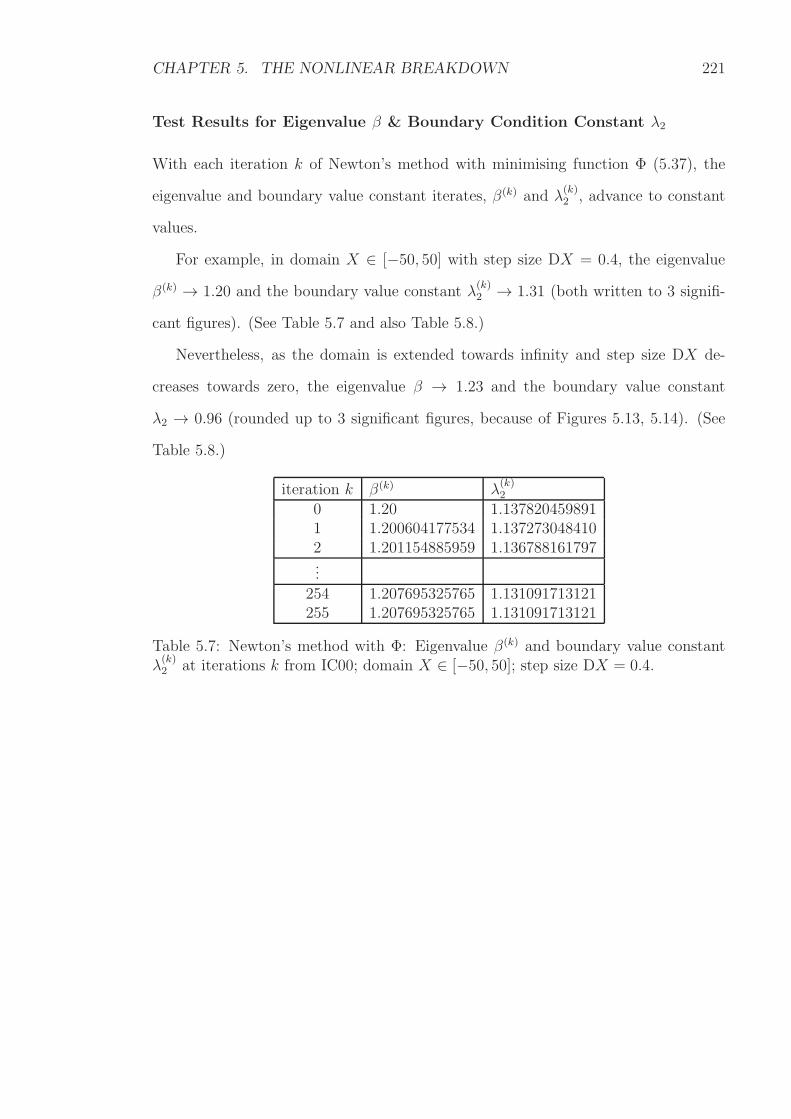
CHAPTER 5. THE NONLINEAR BREAKDOWN 221
Test Results for Eigenvalue β & Boundary Condition Constant λ2
With each iteration k of Newton’s method with minimising function Φ (5.37), the
eigenvalue and boundary value constant iterates, β(k) and λ(k)2 , advance to constant
values.
For example, in domain X ∈ [−50, 50] with step size DX = 0.4, the eigenvalue
β(k) → 1.20 and the boundary value constant λ(k)2 → 1.31 (both written to 3 signifi-
cant figures). (See Table 5.7 and also Table 5.8.)
Nevertheless, as the domain is extended towards infinity and step size DX de-
creases towards zero, the eigenvalue β → 1.23 and the boundary value constant
λ2 → 0.96 (rounded up to 3 significant figures, because of Figures 5.13, 5.14). (See
Table 5.8.)
iteration k β(k) λ(k)2
0 1.20 1.1378204598911 1.200604177534 1.1372730484102 1.201154885959 1.136788161797...
254 1.207695325765 1.131091713121255 1.207695325765 1.131091713121
Table 5.7: Newton’s method with Φ: Eigenvalue β(k) and boundary value constantλ(k)2 at iterations k from IC00; domain X ∈ [−50, 50]; step size DX = 0.4.
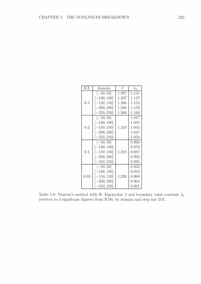
CHAPTER 5. THE NONLINEAR BREAKDOWN 222
DX domain β λ2
0.4
[−50, 50] 1.207 1.131[−100, 100] 1.207 1.147[−150, 150] 1.206 1.154[−200, 200] 1.206 1.159[−250, 250] 1.206 1.160
0.2
[−50, 50]
1.216
1.017[−100, 100] 1.035[−150, 150] 1.043[−200, 200] 1.047[−250, 250] 1.050
0.1
[−50, 50]
1.223
0.960[−100, 100] 0.979[−150, 150] 0.987[−200, 200] 0.992[−250, 250] 0.995
0.05
[−50, 50]
1.226
0.932[−100, 100] 0.952[−150, 150] 0.960[−200, 200] 0.964[−250, 250] 0.967
Table 5.8: Newton’s method with Φ: Eigenvalue β and boundary value constant λ2(written to 4 significant figures) from IC00, by domain and step size DX .
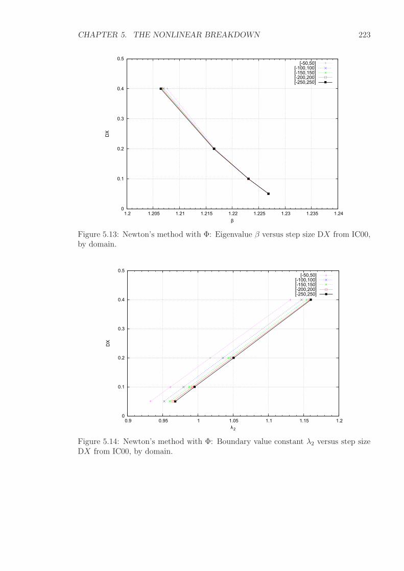
CHAPTER 5. THE NONLINEAR BREAKDOWN 223
0
0.1
0.2
0.3
0.4
0.5
1.2 1.205 1.21 1.215 1.22 1.225 1.23 1.235 1.24
DX
β
[-50,50][-100,100][-150,150][-200,200][-250,250]
Figure 5.13: Newton’s method with Φ: Eigenvalue β versus step size DX from IC00,by domain.
0
0.1
0.2
0.3
0.4
0.5
0.9 0.95 1 1.05 1.1 1.15 1.2
DX
λ2
[-50,50][-100,100][-150,150][-200,200][-250,250]
Figure 5.14: Newton’s method with Φ: Boundary value constant λ2 versus step sizeDX from IC00, by domain.
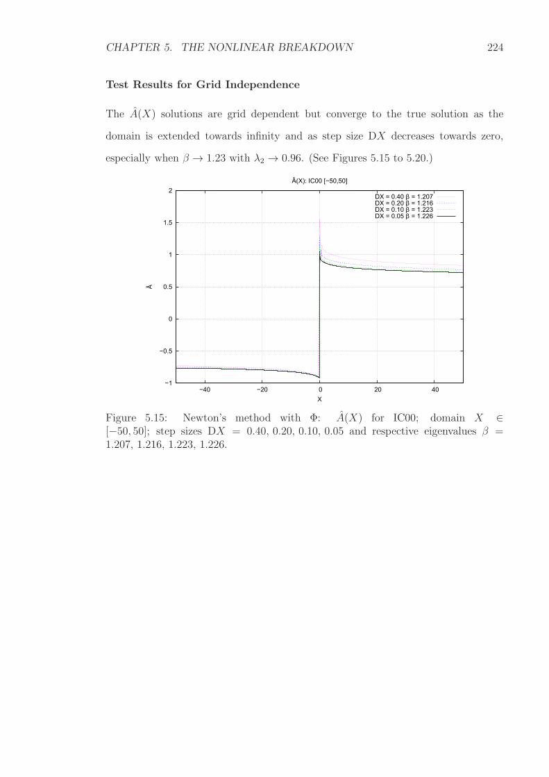
CHAPTER 5. THE NONLINEAR BREAKDOWN 224
Test Results for Grid Independence
The A(X) solutions are grid dependent but converge to the true solution as the
domain is extended towards infinity and as step size DX decreases towards zero,
especially when β → 1.23 with λ2 → 0.96. (See Figures 5.15 to 5.20.)
−1
−0.5
0
0.5
1
1.5
2
−40 −20 0 20 40
Â
X
Â(X): IC00 [−50,50]
DX = 0.40 β = 1.207DX = 0.20 β = 1.216DX = 0.10 β = 1.223DX = 0.05 β = 1.226
Figure 5.15: Newton’s method with Φ: A(X) for IC00; domain X ∈[−50, 50]; step sizes DX = 0.40, 0.20, 0.10, 0.05 and respective eigenvalues β =1.207, 1.216, 1.223, 1.226.
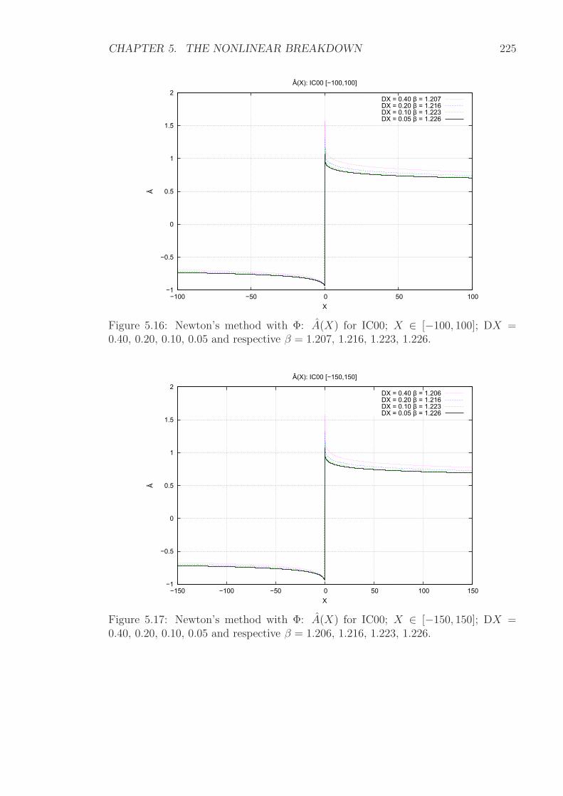
CHAPTER 5. THE NONLINEAR BREAKDOWN 225
−1
−0.5
0
0.5
1
1.5
2
−100 −50 0 50 100
Â
X
Â(X): IC00 [−100,100]
DX = 0.40 β = 1.207DX = 0.20 β = 1.216DX = 0.10 β = 1.223DX = 0.05 β = 1.226
Figure 5.16: Newton’s method with Φ: A(X) for IC00; X ∈ [−100, 100]; DX =0.40, 0.20, 0.10, 0.05 and respective β = 1.207, 1.216, 1.223, 1.226.
−1
−0.5
0
0.5
1
1.5
2
−150 −100 −50 0 50 100 150
Â
X
Â(X): IC00 [−150,150]
DX = 0.40 β = 1.206DX = 0.20 β = 1.216DX = 0.10 β = 1.223DX = 0.05 β = 1.226
Figure 5.17: Newton’s method with Φ: A(X) for IC00; X ∈ [−150, 150]; DX =0.40, 0.20, 0.10, 0.05 and respective β = 1.206, 1.216, 1.223, 1.226.
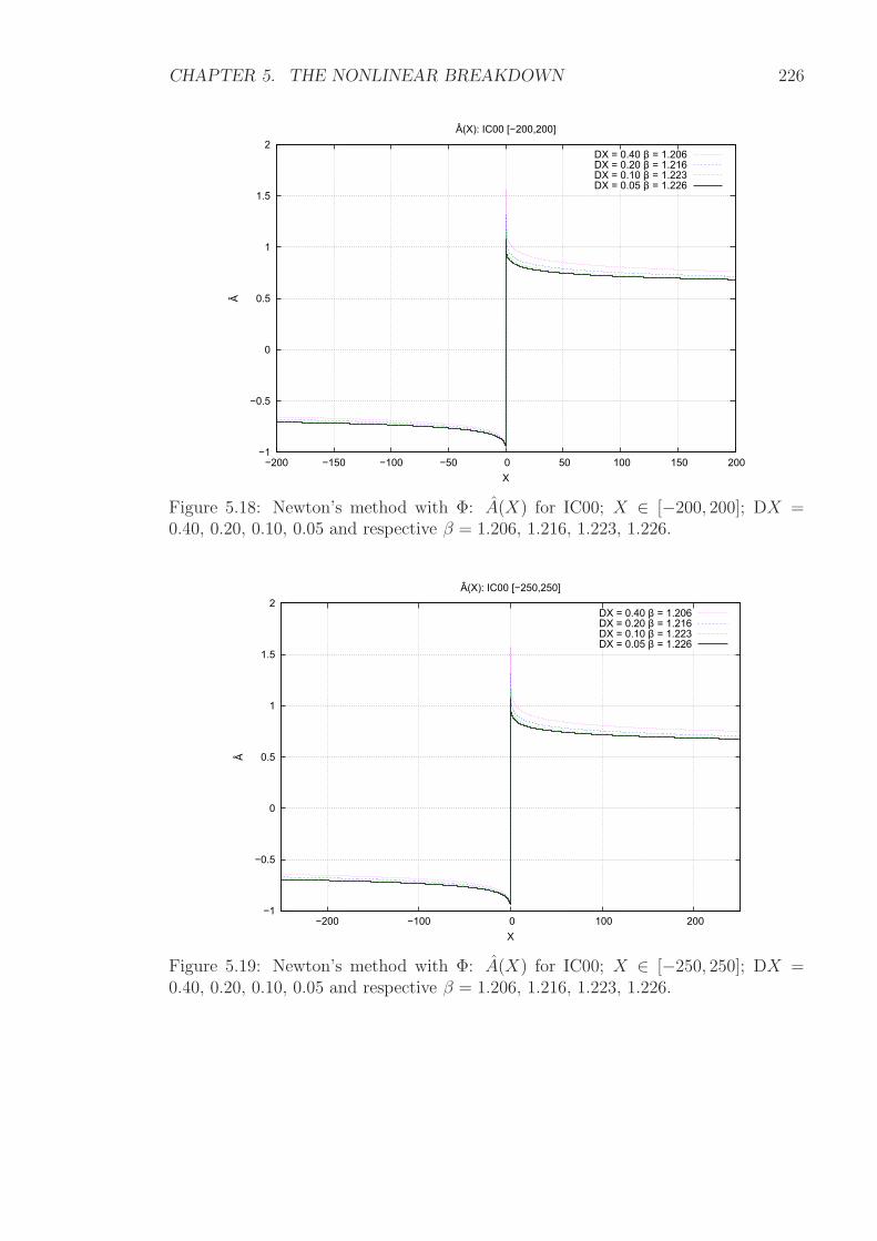
CHAPTER 5. THE NONLINEAR BREAKDOWN 226
−1
−0.5
0
0.5
1
1.5
2
−200 −150 −100 −50 0 50 100 150 200
Â
X
Â(X): IC00 [−200,200]
DX = 0.40 β = 1.206DX = 0.20 β = 1.216DX = 0.10 β = 1.223DX = 0.05 β = 1.226
Figure 5.18: Newton’s method with Φ: A(X) for IC00; X ∈ [−200, 200]; DX =0.40, 0.20, 0.10, 0.05 and respective β = 1.206, 1.216, 1.223, 1.226.
−1
−0.5
0
0.5
1
1.5
2
−200 −100 0 100 200
Â
X
Â(X): IC00 [−250,250]
DX = 0.40 β = 1.206DX = 0.20 β = 1.216DX = 0.10 β = 1.223DX = 0.05 β = 1.226
Figure 5.19: Newton’s method with Φ: A(X) for IC00; X ∈ [−250, 250]; DX =0.40, 0.20, 0.10, 0.05 and respective β = 1.206, 1.216, 1.223, 1.226.
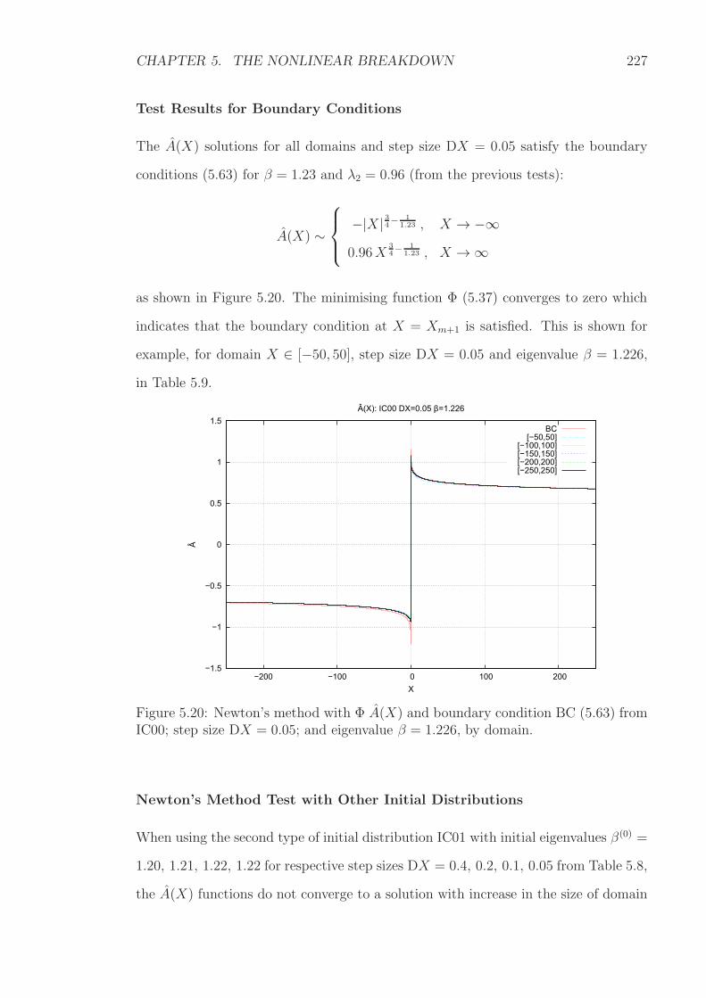
CHAPTER 5. THE NONLINEAR BREAKDOWN 227
Test Results for Boundary Conditions
The A(X) solutions for all domains and step size DX = 0.05 satisfy the boundary
conditions (5.63) for β = 1.23 and λ2 = 0.96 (from the previous tests):
A(X) ∼
−|X| 34− 11.23 , X → −∞
0.96X34− 1
1.23 , X →∞
as shown in Figure 5.20. The minimising function Φ (5.37) converges to zero which
indicates that the boundary condition at X = Xm+1 is satisfied. This is shown for
example, for domain X ∈ [−50, 50], step size DX = 0.05 and eigenvalue β = 1.226,
in Table 5.9.
−1.5
−1
−0.5
0
0.5
1
1.5
−200 −100 0 100 200
Â
X
Â(X): IC00 DX=0.05 β=1.226
BC[−50,50]
[−100,100][−150,150][−200,200][−250,250]
Figure 5.20: Newton’s method with Φ A(X) and boundary condition BC (5.63) fromIC00; step size DX = 0.05; and eigenvalue β = 1.226, by domain.
Newton’s Method Test with Other Initial Distributions
When using the second type of initial distribution IC01 with initial eigenvalues β(0) =
1.20, 1.21, 1.22, 1.22 for respective step sizes DX = 0.4, 0.2, 0.1, 0.05 from Table 5.8,
the A(X) functions do not converge to a solution with increase in the size of domain
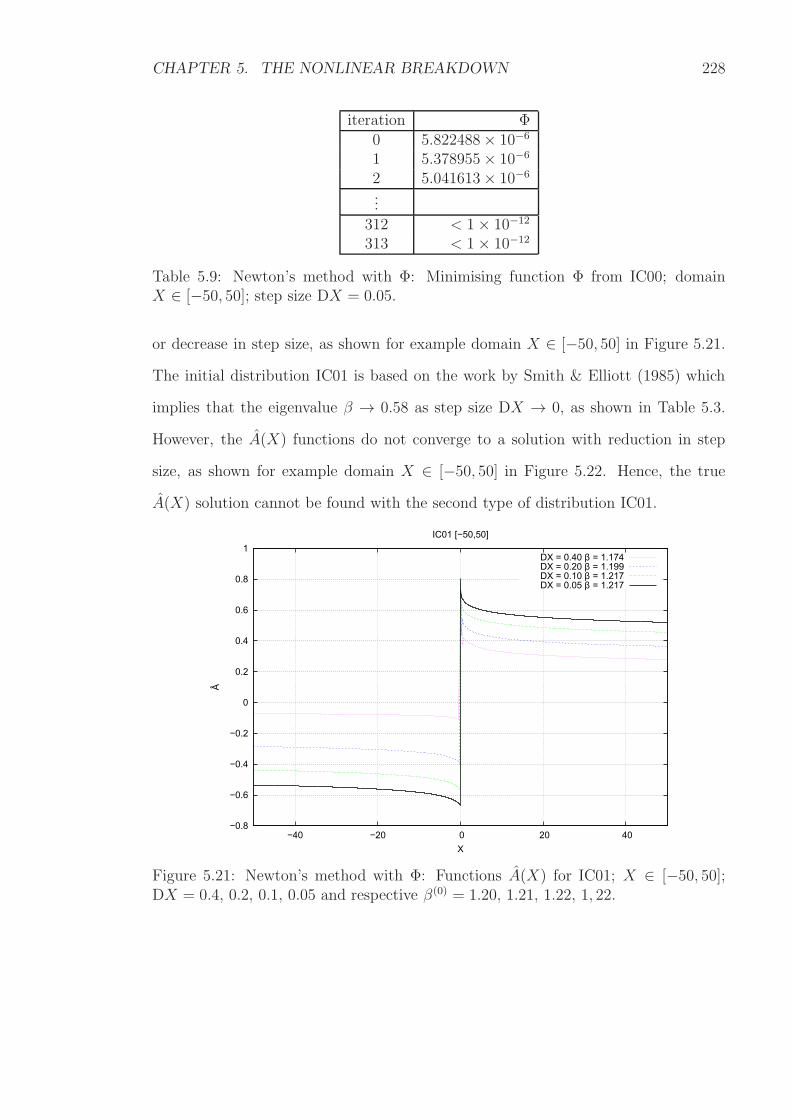
CHAPTER 5. THE NONLINEAR BREAKDOWN 228
iteration Φ0 5.822488× 10⁻⁶
1 5.378955× 10⁻⁶
2 5.041613× 10⁻⁶
...312 < 1× 10⁻¹²
313 < 1× 10⁻¹²
Table 5.9: Newton’s method with Φ: Minimising function Φ from IC00; domainX ∈ [−50, 50]; step size DX = 0.05.
or decrease in step size, as shown for example domain X ∈ [−50, 50] in Figure 5.21.
The initial distribution IC01 is based on the work by Smith & Elliott (1985) which
implies that the eigenvalue β → 0.58 as step size DX → 0, as shown in Table 5.3.
However, the A(X) functions do not converge to a solution with reduction in step
size, as shown for example domain X ∈ [−50, 50] in Figure 5.22. Hence, the true
A(X) solution cannot be found with the second type of distribution IC01.
−0.8
−0.6
−0.4
−0.2
0
0.2
0.4
0.6
0.8
1
−40 −20 0 20 40
Â
X
IC01 [−50,50]
DX = 0.40 β = 1.174DX = 0.20 β = 1.199DX = 0.10 β = 1.217DX = 0.05 β = 1.217
Figure 5.21: Newton’s method with Φ: Functions A(X) for IC01; X ∈ [−50, 50];DX = 0.4, 0.2, 0.1, 0.05 and respective β(0) = 1.20, 1.21, 1.22, 1, 22.
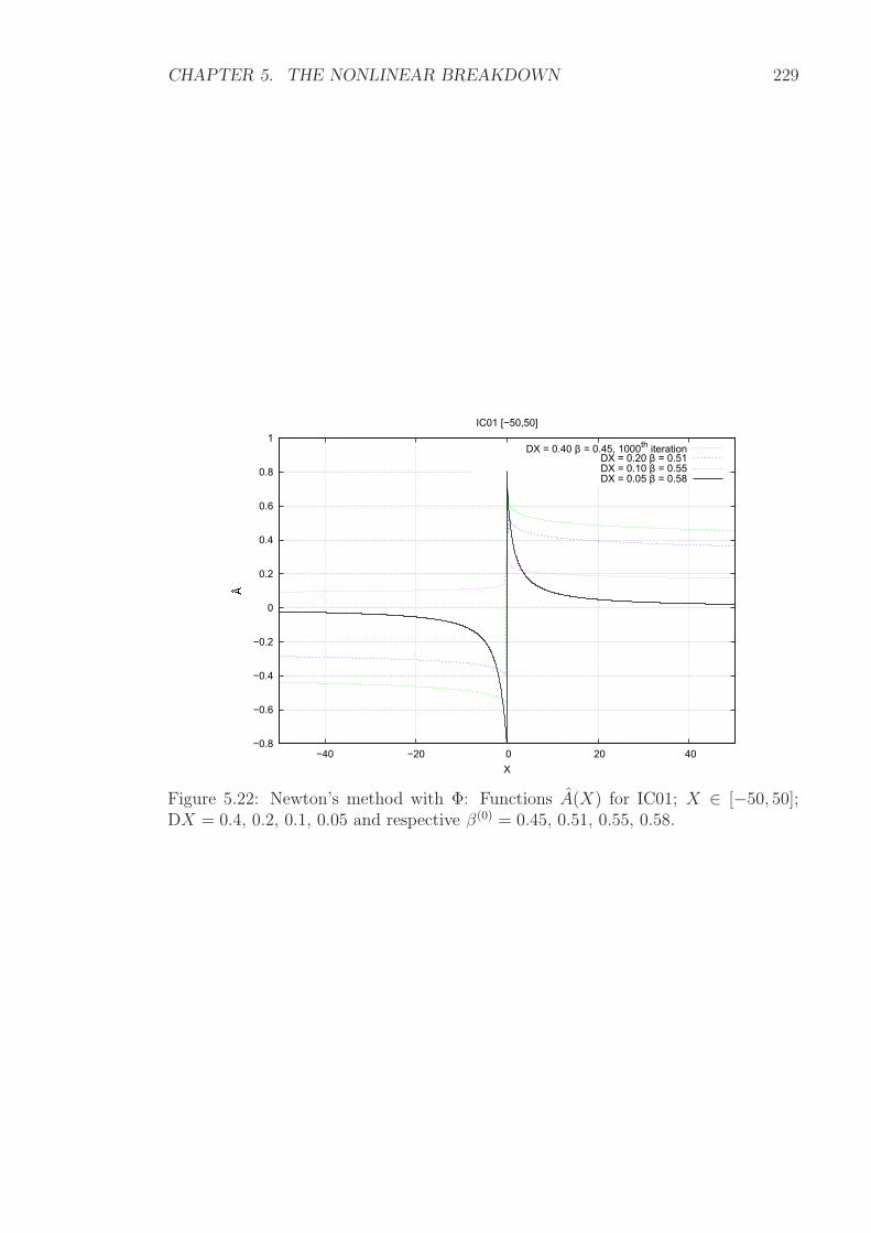
CHAPTER 5. THE NONLINEAR BREAKDOWN 229
−0.8
−0.6
−0.4
−0.2
0
0.2
0.4
0.6
0.8
1
−40 −20 0 20 40
X
IC01 [−50,50]
DX = 0.40 β = 0.45, 1000thiteration
DX = 0.20 β = 0.51DX = 0.10 β = 0.55DX = 0.05 β = 0.58
Figure 5.22: Newton’s method with Φ: Functions A(X) for IC01; X ∈ [−50, 50];DX = 0.4, 0.2, 0.1, 0.05 and respective β(0) = 0.45, 0.51, 0.55, 0.58.
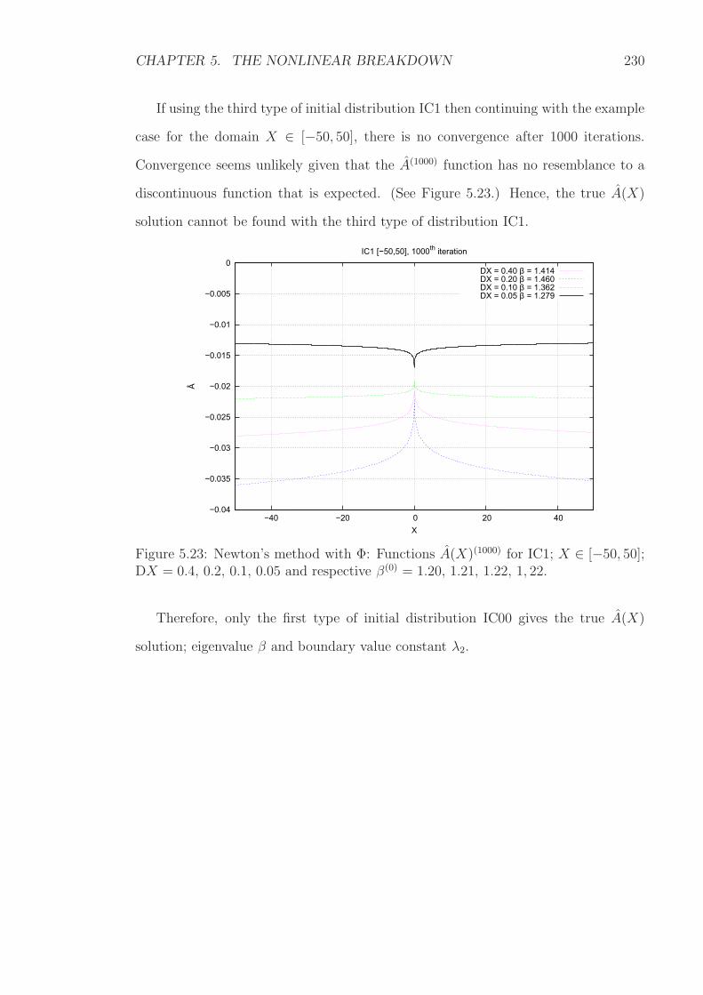
CHAPTER 5. THE NONLINEAR BREAKDOWN 230
If using the third type of initial distribution IC1 then continuing with the example
case for the domain X ∈ [−50, 50], there is no convergence after 1000 iterations.
Convergence seems unlikely given that the A(1000) function has no resemblance to a
discontinuous function that is expected. (See Figure 5.23.) Hence, the true A(X)
solution cannot be found with the third type of distribution IC1.
−0.04
−0.035
−0.03
−0.025
−0.02
−0.015
−0.01
−0.005
0
−40 −20 0 20 40
Â
X
IC1 [−50,50], 1000th iteration
DX = 0.40 β = 1.414DX = 0.20 β = 1.460DX = 0.10 β = 1.362DX = 0.05 β = 1.279
Figure 5.23: Newton’s method with Φ: Functions A(X)(1000) for IC1; X ∈ [−50, 50];DX = 0.4, 0.2, 0.1, 0.05 and respective β(0) = 1.20, 1.21, 1.22, 1, 22.
Therefore, only the first type of initial distribution IC00 gives the true A(X)
solution; eigenvalue β and boundary value constant λ2.
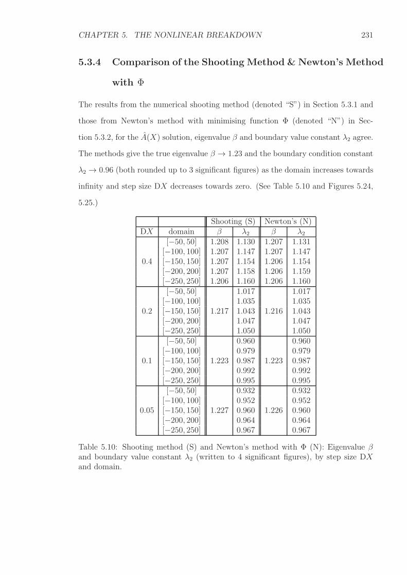
CHAPTER 5. THE NONLINEAR BREAKDOWN 231
5.3.4 Comparison of the Shooting Method & Newton’s Method
with Φ
The results from the numerical shooting method (denoted “S”) in Section 5.3.1 and
those from Newton’s method with minimising function Φ (denoted “N”) in Sec-
tion 5.3.2, for the A(X) solution, eigenvalue β and boundary value constant λ2 agree.
The methods give the true eigenvalue β → 1.23 and the boundary condition constant
λ2 → 0.96 (both rounded up to 3 significant figures) as the domain increases towards
infinity and step size DX decreases towards zero. (See Table 5.10 and Figures 5.24,
5.25.)
Shooting (S) Newton’s (N)DX domain β λ2 β λ2
0.4
[−50, 50] 1.208 1.130 1.207 1.131[−100, 100] 1.207 1.147 1.207 1.147[−150, 150] 1.207 1.154 1.206 1.154[−200, 200] 1.207 1.158 1.206 1.159[−250, 250] 1.206 1.160 1.206 1.160
0.2
[−50, 50]
1.217
1.017
1.216
1.017[−100, 100] 1.035 1.035[−150, 150] 1.043 1.043[−200, 200] 1.047 1.047[−250, 250] 1.050 1.050
0.1
[−50, 50]
1.223
0.960
1.223
0.960[−100, 100] 0.979 0.979[−150, 150] 0.987 0.987[−200, 200] 0.992 0.992[−250, 250] 0.995 0.995
0.05
[−50, 50]
1.227
0.932
1.226
0.932[−100, 100] 0.952 0.952[−150, 150] 0.960 0.960[−200, 200] 0.964 0.964[−250, 250] 0.967 0.967
Table 5.10: Shooting method (S) and Newton’s method with Φ (N): Eigenvalue βand boundary value constant λ2 (written to 4 significant figures), by step size DXand domain.
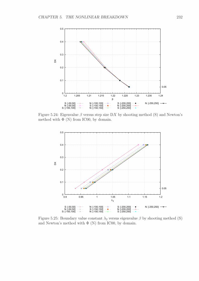
CHAPTER 5. THE NONLINEAR BREAKDOWN 232
0
0.1
0.2
0.3
0.4
0.5
1.2 1.205 1.21 1.215 1.22 1.225 1.23 1.235 1.24
0.05
DX
β
S: [-50,50]N: [-50,50]
S: [-100,100]
N: [-100,100]S: [-150,150]N: [-150,150]
S: [-200,200]N: [-200,200]S: [-250,250]
N: [-250,250]
Figure 5.24: Eigenvalue β versus step size DX by shooting method (S) and Newton’smethod with Φ (N) from IC00, by domain.
0
0.1
0.2
0.3
0.4
0.5
0.9 0.95 1 1.05 1.1 1.15 1.2
0.05
DX
λ2
S: [-50,50]N: [-50,50]
S: [-100,100]
N: [-100,100]S: [-150,150]N: [-150,150]
S: [-200,200]N: [-200,200]S: [-250,250]
N: [-250,250]
Figure 5.25: Boundary value constant λ2 versus eigenvalue β by shooting method (S)and Newton’s method with Φ (N) from IC00, by domain.
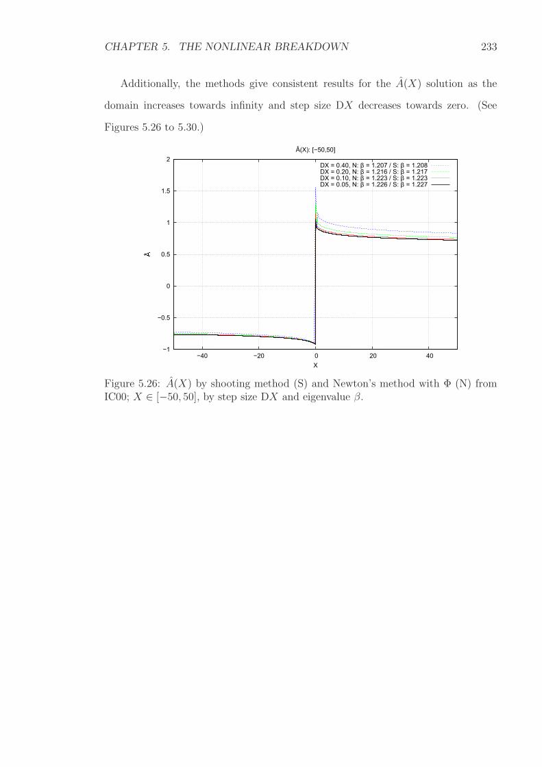
CHAPTER 5. THE NONLINEAR BREAKDOWN 233
Additionally, the methods give consistent results for the A(X) solution as the
domain increases towards infinity and step size DX decreases towards zero. (See
Figures 5.26 to 5.30.)
−1
−0.5
0
0.5
1
1.5
2
−40 −20 0 20 40
X
Â(X): [−50,50]
DX = 0.40, N: β = 1.207 / S: β = 1.208DX = 0.20, N: β = 1.216 / S: β = 1.217DX = 0.10, N: β = 1.223 / S: β = 1.223DX = 0.05, N: β = 1.226 / S: β = 1.227
Figure 5.26: A(X) by shooting method (S) and Newton’s method with Φ (N) fromIC00; X ∈ [−50, 50], by step size DX and eigenvalue β.
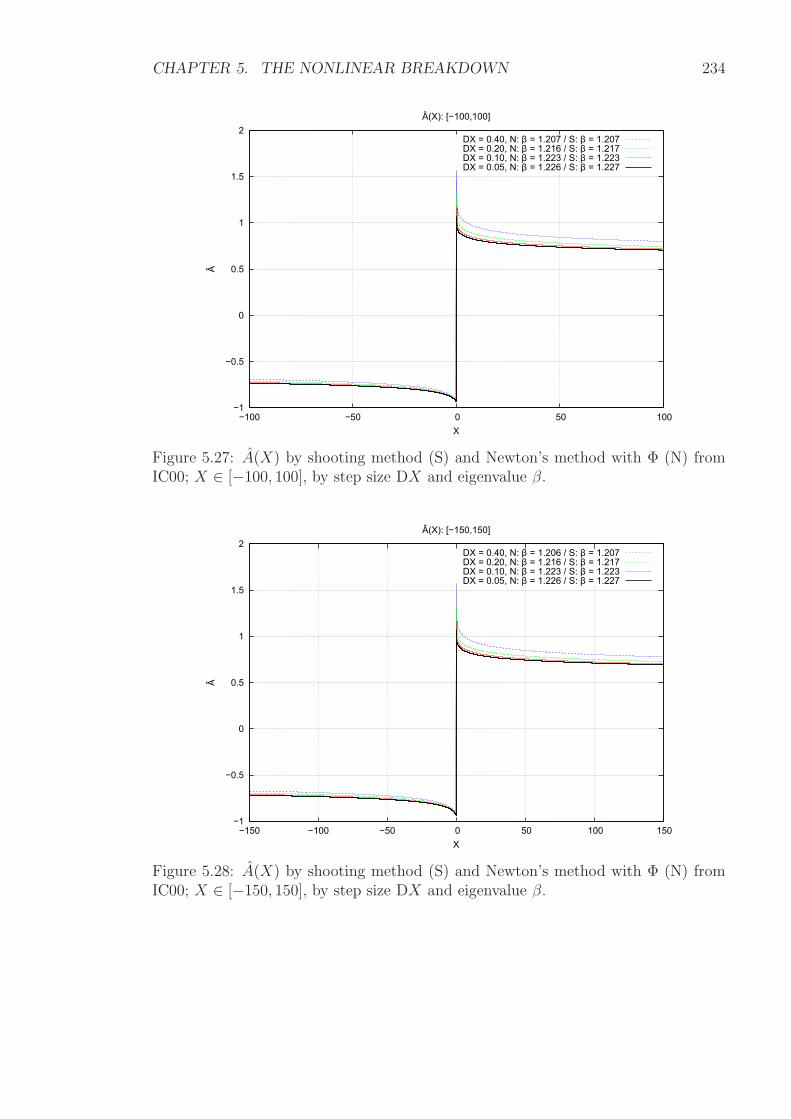
CHAPTER 5. THE NONLINEAR BREAKDOWN 234
−1
−0.5
0
0.5
1
1.5
2
−100 −50 0 50 100
Â
X
Â(X): [−100,100]
DX = 0.40, N: β = 1.207 / S: β = 1.207DX = 0.20, N: β = 1.216 / S: β = 1.217DX = 0.10, N: β = 1.223 / S: β = 1.223DX = 0.05, N: β = 1.226 / S: β = 1.227
Figure 5.27: A(X) by shooting method (S) and Newton’s method with Φ (N) fromIC00; X ∈ [−100, 100], by step size DX and eigenvalue β.
−1
−0.5
0
0.5
1
1.5
2
−150 −100 −50 0 50 100 150
Â
X
Â(X): [−150,150]
DX = 0.40, N: β = 1.206 / S: β = 1.207DX = 0.20, N: β = 1.216 / S: β = 1.217DX = 0.10, N: β = 1.223 / S: β = 1.223DX = 0.05, N: β = 1.226 / S: β = 1.227
Figure 5.28: A(X) by shooting method (S) and Newton’s method with Φ (N) fromIC00; X ∈ [−150, 150], by step size DX and eigenvalue β.
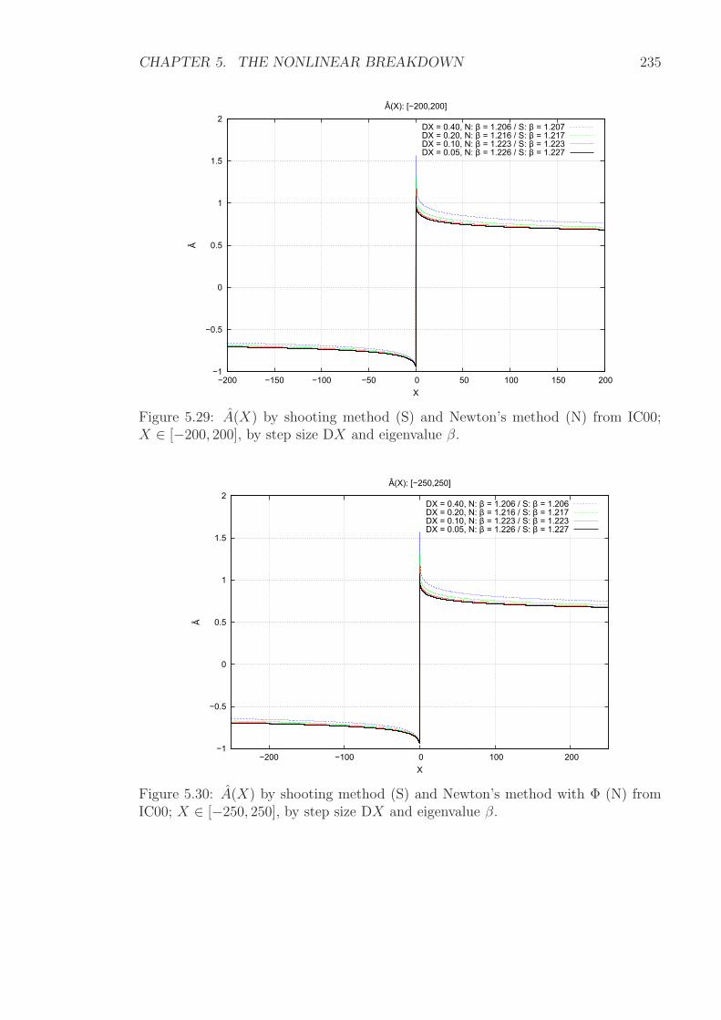
CHAPTER 5. THE NONLINEAR BREAKDOWN 235
−1
−0.5
0
0.5
1
1.5
2
−200 −150 −100 −50 0 50 100 150 200
Â
X
Â(X): [−200,200]
DX = 0.40, N: β = 1.206 / S: β = 1.207DX = 0.20, N: β = 1.216 / S: β = 1.217DX = 0.10, N: β = 1.223 / S: β = 1.223DX = 0.05, N: β = 1.226 / S: β = 1.227
Figure 5.29: A(X) by shooting method (S) and Newton’s method (N) from IC00;X ∈ [−200, 200], by step size DX and eigenvalue β.
−1
−0.5
0
0.5
1
1.5
2
−200 −100 0 100 200
Â
X
Â(X): [−250,250]
DX = 0.40, N: β = 1.206 / S: β = 1.206DX = 0.20, N: β = 1.216 / S: β = 1.217DX = 0.10, N: β = 1.223 / S: β = 1.223DX = 0.05, N: β = 1.226 / S: β = 1.227
Figure 5.30: A(X) by shooting method (S) and Newton’s method with Φ (N) fromIC00; X ∈ [−250, 250], by step size DX and eigenvalue β.
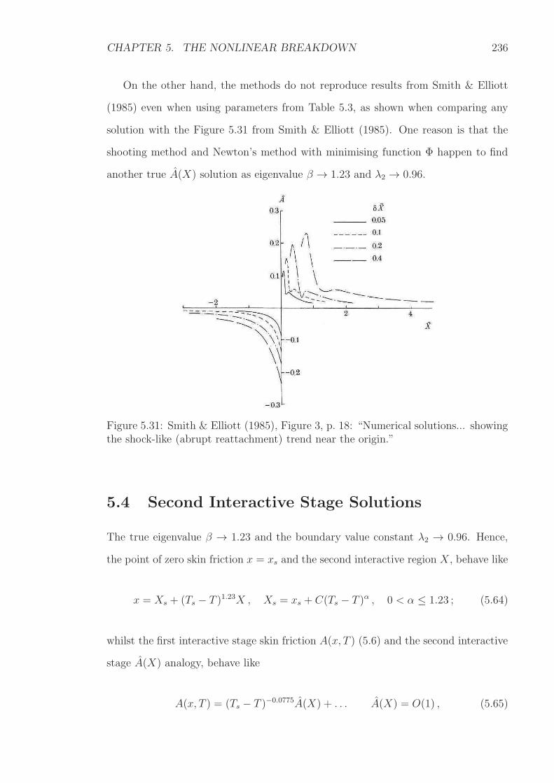
CHAPTER 5. THE NONLINEAR BREAKDOWN 236
On the other hand, the methods do not reproduce results from Smith & Elliott
(1985) even when using parameters from Table 5.3, as shown when comparing any
solution with the Figure 5.31 from Smith & Elliott (1985). One reason is that the
shooting method and Newton’s method with minimising function Φ happen to find
another true A(X) solution as eigenvalue β → 1.23 and λ2 → 0.96.
Figure 5.31: Smith & Elliott (1985), Figure 3, p. 18: “Numerical solutions... showingthe shock-like (abrupt reattachment) trend near the origin.”
5.4 Second Interactive Stage Solutions
The true eigenvalue β → 1.23 and the boundary value constant λ2 → 0.96. Hence,
the point of zero skin friction x = xs and the second interactive region X , behave like
x = Xs + (Ts − T )1.23X , Xs = xs + C(Ts − T )α , 0 < α ≤ 1.23 ; (5.64)
whilst the first interactive stage skin friction A(x, T ) (5.6) and the second interactive
stage A(X) analogy, behave like
A(x, T ) = (Ts − T )−0.0775A(X) + . . . A(X) = O(1) , (5.65)
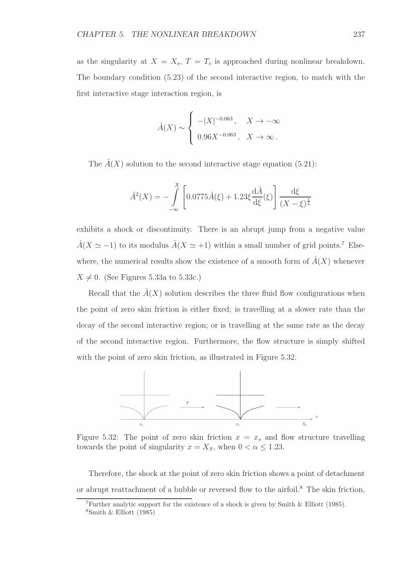
CHAPTER 5. THE NONLINEAR BREAKDOWN 237
as the singularity at X = Xs, T = Ts is approached during nonlinear breakdown.
The boundary condition (5.23) of the second interactive region, to match with the
first interactive stage interaction region, is
A(X) ∼
−|X|−0.063 , X → −∞
0.96X−0.063 , X →∞ .
The A(X) solution to the second interactive stage equation (5.21):
A2(X) = −X∫
−∞
[
0.0775A(ξ) + 1.23ξdA
dξ(ξ)
]
dξ
(X − ξ) 14
exhibits a shock or discontinuity. There is an abrupt jump from a negative value
A(X ≃ −1) to its modulus A(X ≃ +1) within a small number of grid points.7 Else-
where, the numerical results show the existence of a smooth form of A(X) whenever
X 6= 0. (See Figures 5.33a to 5.33c.)
Recall that the A(X) solution describes the three fluid flow configurations when
the point of zero skin friction is either fixed; is travelling at a slower rate than the
decay of the second interactive region; or is travelling at the same rate as the decay
of the second interactive region. Furthermore, the flow structure is simply shifted
with the point of zero skin friction, as illustrated in Figure 5.32.
Xs
x
xs xs
T
Figure 5.32: The point of zero skin friction x = xs and flow structure travellingtowards the point of singularity x = XS, when 0 < α ≤ 1.23.
Therefore, the shock at the point of zero skin friction shows a point of detachment
or abrupt reattachment of a bubble or reversed flow to the airfoil.8 The skin friction,
7Further analytic support for the existence of a shock is given by Smith & Elliott (1985).8Smith & Elliott (1985)
CHAPTER 5. THE NONLINEAR BREAKDOWN 238
being negative for X < 0, shows forward attached flow; and being positive for X >
0, shows reversed flow in the closed bubble. The shock can either be stationary
or travelling along the airfoil towards a point of singularity. Coinciding with the
decay of the second interactive region is the increasing accentuation of the bubble
which thickens the boundary layer. Eventually, the flow scale returns to that of the
boundary layer as the bubble spans the entire layer. This is analysed in Chapter 6
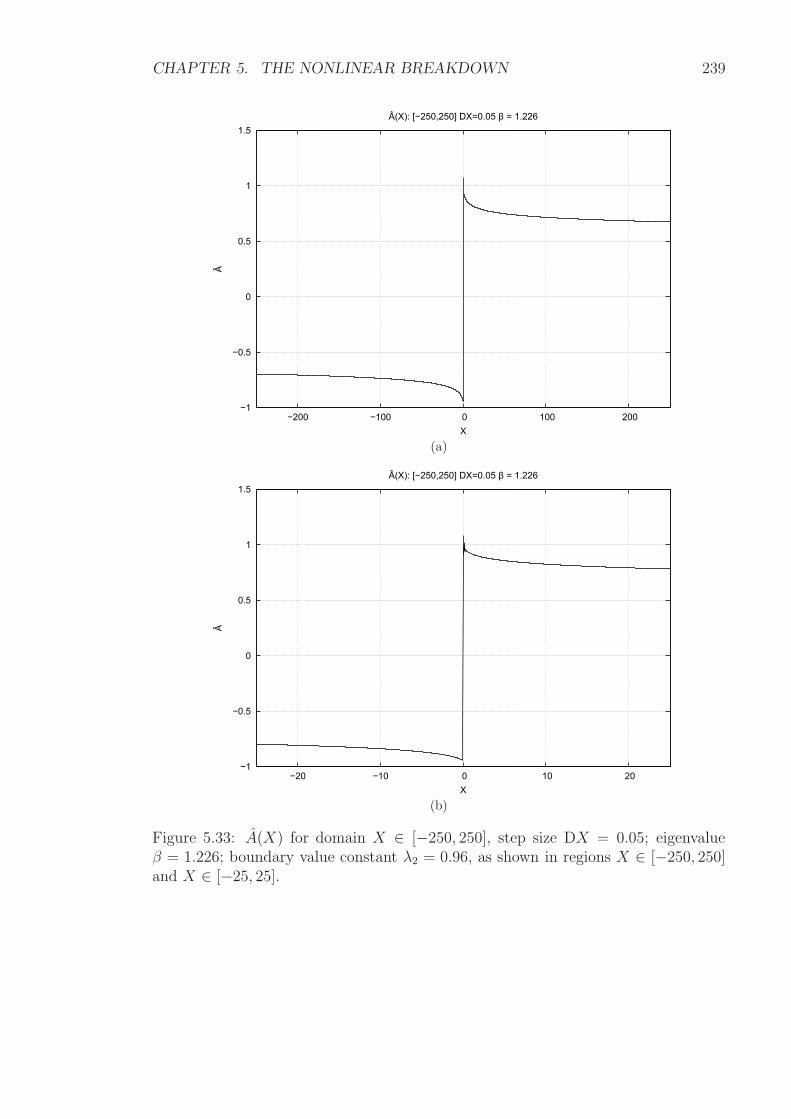
CHAPTER 5. THE NONLINEAR BREAKDOWN 239
−1
−0.5
0
0.5
1
1.5
−200 −100 0 100 200
Â
X
Â(X): [−250,250] DX=0.05 β = 1.226
(a)
−1
−0.5
0
0.5
1
1.5
−20 −10 0 10 20
Â
X
Â(X): [−250,250] DX=0.05 β = 1.226
(b)
Figure 5.33: A(X) for domain X ∈ [−250, 250], step size DX = 0.05; eigenvalueβ = 1.226; boundary value constant λ2 = 0.96, as shown in regions X ∈ [−250, 250]and X ∈ [−25, 25].
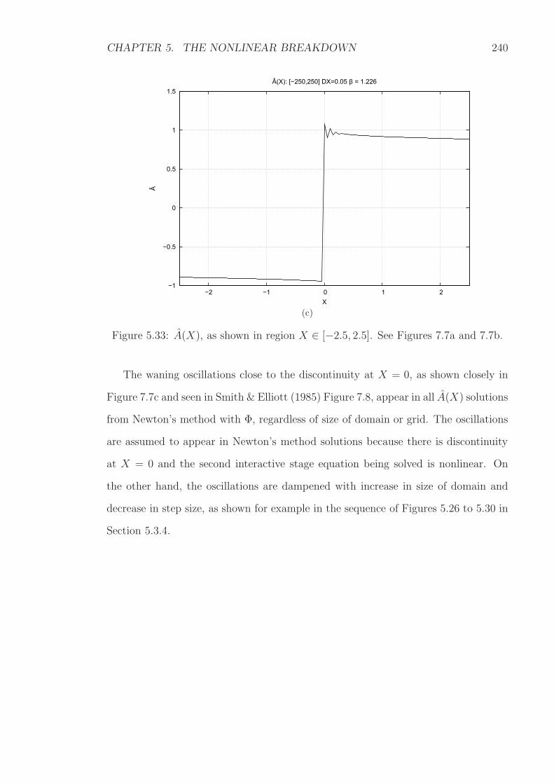
CHAPTER 5. THE NONLINEAR BREAKDOWN 240
−1
−0.5
0
0.5
1
1.5
−2 −1 0 1 2
Â
X
Â(X): [−250,250] DX=0.05 β = 1.226
(c)
Figure 5.33: A(X), as shown in region X ∈ [−2.5, 2.5]. See Figures 7.7a and 7.7b.
The waning oscillations close to the discontinuity at X = 0, as shown closely in
Figure 7.7c and seen in Smith & Elliott (1985) Figure 7.8, appear in all A(X) solutions
from Newton’s method with Φ, regardless of size of domain or grid. The oscillations
are assumed to appear in Newton’s method solutions because there is discontinuity
at X = 0 and the second interactive stage equation being solved is nonlinear. On
the other hand, the oscillations are dampened with increase in size of domain and
decrease in step size, as shown for example in the sequence of Figures 5.26 to 5.30 in
Section 5.3.4.
Chapter 6
Leading Edge Stall
The process of leading edge stall continues from the second interactive stage nonlinear
breakdown (Chapter 5), where there is runaway growth of a bubble of reversed flow
and discontinuous skin friction advancing towards a singularity. The induced pressure
gradient (Section 3.1), that was made negligible in the interaction region by the slow
perturbations to the airfoil on a large time scale T , exists in the unsteady interactive
structure, regardless of the time scale on which the structure exists. Ultimately, the
flow regime is that where time and length scales shorten to the scale of boundary
layer thickness. The flow reaches a nonlinear Euler stage where the growth of the
bubble spans the boundary layer. Evidence for the terminal flow is from analysis of
the leading edge, starting with the boundary layer and its governing equations. The
analysis follows from that of dynamic stall due to unsteady marginal separation by
Elliott & Smith (1987), which has been adapted here.
6.1 The Unsteady Boundary Layer
The boundary layer has the normal coordinate (2.8):
Y = Re12y = O(1) , (6.1)
241
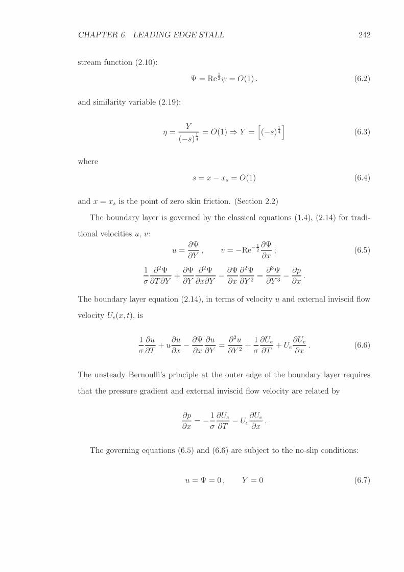
CHAPTER 6. LEADING EDGE STALL 242
stream function (2.10):
Ψ = Re12ψ = O(1) . (6.2)
and similarity variable (2.19):
η =Y
(−s) 14
= O(1)⇒ Y =[
(−s) 14
]
(6.3)
where
s = x− xs = O(1) (6.4)
and x = xs is the point of zero skin friction. (Section 2.2)
The boundary layer is governed by the classical equations (1.4), (2.14) for tradi-
tional velocities u, v:
u =∂Ψ
∂Y, v = −Re− 1
2∂Ψ
∂x; (6.5)
1
σ
∂2Ψ
∂T∂Y+∂Ψ
∂Y
∂2Ψ
∂x∂Y− ∂Ψ
∂x
∂2Ψ
∂Y 2=∂3Ψ
∂Y 3− ∂p
∂x.
The boundary layer equation (2.14), in terms of velocity u and external inviscid flow
velocity Ue(x, t), is
1
σ
∂u
∂T+ u
∂u
∂x− ∂Ψ
∂x
∂u
∂Y=∂2u
∂Y 2+
1
σ
∂Ue
∂T+ Ue
∂Ue
∂x. (6.6)
The unsteady Bernoulli’s principle at the outer edge of the boundary layer requires
that the pressure gradient and external inviscid flow velocity are related by
∂p
∂x= −1
σ
∂Ue
∂T− Ue
∂Ue
∂x.
The governing equations (6.5) and (6.6) are subject to the no-slip conditions:
u = Ψ = 0 , Y = 0 (6.7)
CHAPTER 6. LEADING EDGE STALL 243
and the condition of matching with the external inviscid region:
Ψ ∼ Ue(x, t)[Y − δ∗] , u =∂Ψ
∂Y→ Ue(x, t) , Y →∞ (6.8)
where
δ∗ = Re−12 δ(x, t) (6.9)
is the boundary layer displacement. Given a suitable initial condition, the problem
(6.6), (6.7), (6.8) can be solved.
Length Scales
A nonlinear-unsteady-viscous balance of forces in the boundary layer equation (6.6)
gives
u∂u
∂x∼ ∂p
∂x⇒ p = O(u2) , (6.10)
u∂u
∂x∼ ∂2u
∂Y 2⇒ u = O
[
(−s)Y 2
]
, (6.11)
1
σ
∂u
∂T∼ ∂2u
∂Y 2⇒ Y = O
[
(σT )12
]
. (6.12)
The boundary layer solution of (6.6) has a well-known tangential velocity profile
at separation with the behaviour (2.43):
u = u0(Y ) ∼1
2λ0Y
2 = O(Y 2) , Y → 0 , (6.13)
u0(Y )→ Ue(xs) , Y →∞ .
The boundary layer profile is assumed to be simply displaced which then rides
over the viscous sublayer. This is because any induced pressure gradient, from the
displacement of the boundary layer, is simply transmitted across the middle layer of
the interaction region, according to (3.17). The boundary layer displacement in Y is
CHAPTER 6. LEADING EDGE STALL 244
a small change to the separation profile u = u0(Y ), like
∆u = O[
(−s) 14
]
(6.14)
due to a small change in similarity variable (6.3): ∆Y = O[(−s) 14 ]. Similarly, the
boundary layer displacement gives rise to a normal velocity v at the outer edge of the
boundary layer (Y →∞), which behaves like:1
v = O[
Re−12 (−s)− 3
4
]
. (6.15)
Therefore, by combining (6.13) and (6.3):
u = O[
(−s) 12
]
; (6.16)
by combining (6.10) and (6.3):
p = O [(−s)] ; (6.17)
and by combining (6.12) and (6.16):
T = O
[
(−s)σ
]
, (6.18)
for length scale s (6.4) and time parameter σ →∞.
6.2 The Interaction Region
As the point of zero skin friction x = xs is approached and (−s)→ 0, the boundary
layer theory breaks down and there is an interaction region where displacement of the
boundary layer becomes the same order of magnitude as the boundary layer itself.
1See also Elliott & Smith (1987).
CHAPTER 6. LEADING EDGE STALL 245
The interaction region has time and length scales:
t− σT = O(1) , (−s) = O(
σ−4)
, O(σ) > O(
Re120
)
; Re , σ →∞ (6.19)
such that induced pressure gradient from the displacement of the boundary layer is
negligible. (Chapter 3) In particular, the length scale (3.10) or (3.18) is
s∗ = x∗ − xs = σ4s = O(1) . (6.20)
If O(σ)→ O(
Re120
)
, the induced pressure gradient returns to the flow.
Recall that the flow structure of the interaction region is consistent if the solv-
ability condition (4.1) for skin friction A(x, T ):
A2(x, T )− x2 + 2a(T ) = − 234
Γ(54)
x∫
−∞
∂A
∂T(ξ, T )
dξ
(x− ξ) 14
is satisfied. (Chapter 4) Furthermore, a second interactive stage nonlinear breakdown
occurs on a faster time scale and shorter length scale like (5.64) and (5.65) as a
singularity in A(x, T ) is approached. (Chapter 5)
There is an unsteady interactive region coinciding with the nonlinear breakdown
and the runaway growth of bubble of reversed flow from the solutions of the A(x, T )
equation.
6.3 An Unsteady Interactive Structure
An interactive structure may be constructed, to smooth the singular behaviour in
normal velocity (6.15). The pressure induced by the normal velocity must be com-
parable to the pressure needed to drive the viscous sublayer. Any induced pressure
gradient which perturbs the separation profile and the normal velocity must be of
CHAPTER 6. LEADING EDGE STALL 246
the same order. Hence, from (6.17) and (6.15):
(−s) = O(
Re−27
)
. (6.21)
Therefore, there is an interactive structure of length scale (6.21):
x− xs − σ−4x∗ = Re−27 X , (6.22)
spanning the boundary layer (6.4) and interaction region (6.20) length scales. The
normal coordinate (6.1), similarity variable (6.3) and length scale (6.21) imply y =
Re−12− 1
4· 27 Y . Hence, the normal coordinate of the new region is
y = Re−47 Y , Y = Re−
114 Y . (6.23)
By combining (6.18), (6.19) and (6.21), the time scale in which the new region exists
is
t = σT , T = Re−17 · σ−1T (6.24)
such that
t− σT = Re−17 T . (6.25)
The profile at separation (6.13) implies Ψ = O(Y 3) then combining with (6.3)
and (6.21) gives Ψ = Re34·− 2
7 Ψ. Hence,
ψ = Re−12Ψ Ψ = Re−
314 Ψ . (6.26)
Similarly, (6.16) and (6.21) combine to give
u = Re−17 U . (6.27)
CHAPTER 6. LEADING EDGE STALL 247
Finally, (6.17) and (6.21) combine to give
p = Re−27 P . (6.28)
The boundary layer displacement (6.9) is assumed to have an asymptotic series
expansion of the form:2
δ∗(x, t) = Re−12 δ0 − Re−
47 A(X, T ) + . . .
and hence,
δ∗(x, t) = Re−12 [δ0 − Re−
114 A(X, T ) + . . .] . (6.29)
The A(X, T ) term is the displacement correlation in Y of the same order of magnitude
as the perturbation to the boundary layer ∆Y (6.23). It is analogous to the skin
friction which determines the size of the bubble of reversed flow on the airfoil.
Thus, there is an unsteady interactive structure with the variables X (6.22) and
T (6.25):
x− xs − Re−15x∗ = Re−
27 X , t− σT = Re−
17 T . (6.30)
The boundary layer equation (6.6) becomes:
∂U
∂T+ U
∂U
∂X− ∂Ψ
∂X
∂U
∂Y=∂2U
∂Y 2− ∂P
∂X. (6.31)
It is subject to the no-slip conditions:
U = Ψ = 0 , Y = 0 ;
the condition of matching of the viscous flow to the displaced flow:3
Ψ ∼ 1
6λ0[
Y + A(X, T )]3
+ . . . Y →∞ , (6.32)
2See also Elliott & Smith (1987).3See also Elliott & Smith (1987).
CHAPTER 6. LEADING EDGE STALL 248
and the condition of matching to the attached boundary layer upstream and down-
stream:
U → 1
2λ0Y
2 ,∂P
∂X→ λ0 , |X| → ∞ . (6.33)
The condition of matching (6.32) is obtained from the profile at separation (6.13)
in the variables (6.30), assuming there is simple displacement A(X, T ) in Y of the
unsteady region. The condition (6.33) matches the pressure gradient to the classical
boundary layer pressure gradient λ0 (2.15).
Finally, there is also the subsonic pressure-displacement relation:4
∂P
∂X(X, T ) =
1
π−∞∫
−∞
∂2A
∂ξ2(ξ, T )
dξ
(X − ξ) . (6.34)
Without it, the problem is not closed since the pressure term on the right hand
side of (6.31) remains unknown. The subsonic pressure-displacement relation is due
to the interaction between the boundary layer and external inviscid potential flow.
Importantly, it signifies the existence of an induced pressure gradient on the length
and time scales (6.30) which was otherwise removed from the interaction region by
a slow change in angle of attack on a large time scale (6.19). The interaction region
without an induced pressure gradient does not have an upper layer, as discussed in
Section 3.4. Therefore, with the existence of the induced pressure gradient is the
return to classical triple deck theory.
6.4 The Finite-Time Breakdown Problem
Ultimately, the bubble of reversed flow spans the boundary layer such that the time
and length scales shorten to the scale of boundary layer thickness. The flow reaches
a nonlinear Euler stage.
Assuming that the displacement A(X, T ) of the boundary layer becomes large,
4A subsonic pressure-displacement relation (3.50) obtained in Section 3.4 is derived from theintegral of small perturbation theory (B.6) in Appendix B.
CHAPTER 6. LEADING EDGE STALL 249
then balancing terms from the condition of matching (6.32) of the viscous flow to the
displaced flow, the variables are of order:
Y = O(A) , Ψ = O(A3) , U = O(A2) , Y →∞ . (6.35)
The balance of unsteady-inertial-pressure forces in the governing equation (6.31)
reveals:
∂U
∂T∼ U
∂U
∂X⇒ T ∼ X · A−2 (6.36)
∂U
∂T∼ ∂Ψ
∂X
∂U
∂Y⇒ T ∼ X · A−2 (6.37)
∂U
∂T∼ ∂P
∂X⇒ T ∼ X · P−1 · A−2 . (6.38)
In order for (6.36), (6.37) and (6.38) to be consistent, then
P = O(A4) . (6.39)
Furthermore, if |X| and |T | are chosen to be5
X = O(A−3) , T = O(A−5) (6.40)
such that (6.36), (6.37) and (6.38) remain true and that there is a runaway effect on
the time and length scales as displacement parameter A grows large, then the O(1)
viscous term: ∂2U∂Y 2 cannot be balanced.
Therefore, to leading order, there is an inviscid structure with a fast time scale
and length scale:
X = O(T− 35 ) , Y = O(T− 1
5 ) . (6.41)
Furthermore, there is a bursting effect of the viscous sublayer as T → 0. The gov-
erning equations are
U =∂Ψ
∂Y; (6.42)
5See also Elliott & Smith (1987).
CHAPTER 6. LEADING EDGE STALL 250
∂U
∂T+ U
∂U
∂X− ∂Ψ
∂X
∂U
∂Y= − ∂P
∂X, (6.43)
subject to the inviscid constraint of tangential flow:
Ψ = O(Y ) , Y → 0 ;
the condition of matching to the external inviscid flow:
Ψ ∼ 1
6λ0[
Y + A(X, T )]3
+ . . . Y →∞ ;
and the pressure displacement law: (6.34). The finite-time breakdown problem, con-
sisting of equations (6.42), (6.43) and their conditions, holds as long as a viscous
sublayer exists which brings the fluid flow velocity to rest at the surface. The prob-
lem continues from the analogous problem by Smith (1982a) such that there is a
continuing increase of reversed flow associated with increase in A.
According to the analysis, there is a short-scale breakdown with |X − X0| ∼
|T − T0|35 , and with the viscous flow splitting into two.6 There is an external inviscid
part which erupts like Y ∼ |T − T0|−15 and a diminishing inner viscous region with
Y ∼ |T− T0|−12 (derived from the nonlinear-unsteady-viscous balance in the unsteady
boundary layer equation (6.31); similar to (6.12)). Eventually the external region will
be indistinguishable from the majority of the boundary layer of thickness O(Re−12 ).
This occurs when the Eulerian scalings:
t− σT − Re−17 T0 = O
(
Re−12
)
(6.44)
x− xs − Re15x∗ − Re−
27 X0 = O
(
Re−12
)
are true. The velocity and pressure disturbances become increased to order unity
and so the Euler equations come into operation across the entire boundary layer. A
vortex starts to span the boundary layer and its evolution becomes a vortex sheet
6See also Elliott & Smith (1987).

CHAPTER 6. LEADING EDGE STALL 251
problem.
The effects described in this Chapter mark the end of the second interactive stage
of the thickening of the boundary layer and the start of a third interactive stage where
there is unsteady vortex development and ejection. The third interactive stage is the
process of leading edge stall.
Chapter 7
Summary & Conclusions
The thesis aimed to bridge the work on marginal separation with that on steady flow
over a downstream-moving surface, unsteady marginal separation and dynamic stall.
In particular, the focus was on the quasi-steady flow structure which develops over a
very large time scale when there are very slow perturbations to the otherwise steady
stream functions. The slow perturbations are from a slow change in angle of attack
over a small range as it gradually approaches the critical angle where stream function
solutions become complex and nonlinear breakdown occurs. (See Figure 7.1.)
The original work comprises of manipulating marginal separation theory, where
the angle of attack is altered to reduce the strength of an adverse pressure gradient
and Goldstein’s singularity, to include the effects of slow perturbations and change
in angle of attack on a large time scale as to render induced pressure gradient neg-
ligible in the interaction region. In short, the fundamental equation of unsteady
marginal separation (1.11) for skin friction loses the term representing the pressure-
displacement relation from the induced pressure gradient and notably, gains an un-
steady term representing the slow change in angle of attack. The unsteady term
ultimately comes from making the first constant in the largest perturbation of the
steady stream function solution, a function of the large time scale and assigning the
change in angle of attack to it. Solutions to the equation are found. The subsequent
finite-time, nonlinear breakdown equation is shown to allow another discontinuous
252
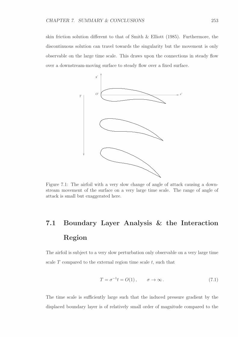
CHAPTER 7. SUMMARY & CONCLUSIONS 253
skin friction solution different to that of Smith & Elliott (1985). Furthermore, the
discontinuous solution can travel towards the singularity but the movement is only
observable on the large time scale. This draws upon the connections in steady flow
over a downstream-moving surface to steady flow over a fixed surface.
y’
O’ x’T
Figure 7.1: The airfoil with a very slow change of angle of attack causing a down-stream movement of the surface on a very large time scale. The range of angle ofattack is small but exaggerated here.
7.1 Boundary Layer Analysis & the Interaction
Region
The airfoil is subject to a very slow perturbation only observable on a very large time
scale T compared to the external region time scale t, such that
T = σ−1t = O(1) , σ →∞ . (7.1)
The time scale is sufficiently large such that the induced pressure gradient by the
displaced boundary layer is of relatively small order of magnitude compared to the
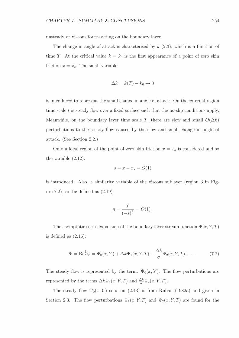
CHAPTER 7. SUMMARY & CONCLUSIONS 254
unsteady or viscous forces acting on the boundary layer.
The change in angle of attack is characterised by k (2.3), which is a function of
time T . At the critical value k = k0 is the first appearance of a point of zero skin
friction x = xs. The small variable:
∆k = k(T )− k0 → 0
is introduced to represent the small change in angle of attack. On the external region
time scale t is steady flow over a fixed surface such that the no-slip conditions apply.
Meanwhile, on the boundary layer time scale T , there are slow and small O(∆k)
perturbations to the steady flow caused by the slow and small change in angle of
attack. (See Section 2.2.)
Only a local region of the point of zero skin friction x = xs is considered and so
the variable (2.12):
s = x− xs = O(1)
is introduced. Also, a similarity variable of the viscous sublayer (region 3 in Fig-
ure 7.2) can be defined as (2.19):
η =Y
(−s) 14
= O(1) .
The asymptotic series expansion of the boundary layer stream function Ψ(x, Y, T )
is defined as (2.16):
Ψ = Re12ψ = Ψ0(x, Y ) + ∆kΨ1(x, Y, T ) +
∆k
σΨ2(x, Y, T ) + . . . (7.2)
The steady flow is represented by the term: Ψ0(x, Y ). The flow perturbations are
represented by the terms ∆kΨ1(x, Y, T ) and∆kσΨ2(x, Y, T ).
The steady flow Ψ0(x, Y ) solution (2.43) is from Ruban (1982a) and given in
Section 2.3. The flow perturbations Ψ1(x, Y, T ) and Ψ2(x, Y, T ) are found for the
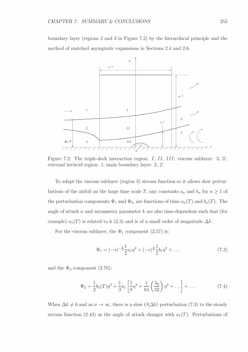
CHAPTER 7. SUMMARY & CONCLUSIONS 255
boundary layer (regions 2 and 3 in Figure 7.2) by the hierarchical principle and the
method of matched asymptotic expansions in Sections 2.4 and 2.6.
1
2
2’
3’
0
III
II
I
σ−4
y
Re−12 3
σ−1
σ−4
x
Figure 7.2: The triple-deck interaction region: I, II, III; viscous sublayer: 3, 3’;external inviscid region: 1; main boundary layer: 2, 2’.
To adapt the viscous sublayer (region 3) stream function so it allows slow pertur-
bations of the airfoil on the large time scale T , any constants an and bn for n ≥ 1 of
the perturbation components Ψ1 and Ψ2, are functions of time an(T ) and bn(T ). The
angle of attack α and asymmetry parameter k are also time-dependent such that (for
example) a1(T ) is related to k (2.3) and is of a small order of magnitude ∆k.
For the viscous sublayer, the Ψ1 component (2.57) is:
Ψ1 = (−s)− 121
2a1η
2 + (−s) 141
2b1η
2 + . . . (7.3)
and the Ψ2 component (2.76):
Ψ2 =1
2b2(T )η
2 +1
3a1
[
1
8η4 +
1
84
(
λ032
)
η8 + . . .
]
+ . . . (7.4)
When ∆k 6= 0 and as σ →∞, there is a slow O(∆k) perturbation (7.3) to the steady
stream function (2.43) as the angle of attack changes with a1(T ). Perturbations of
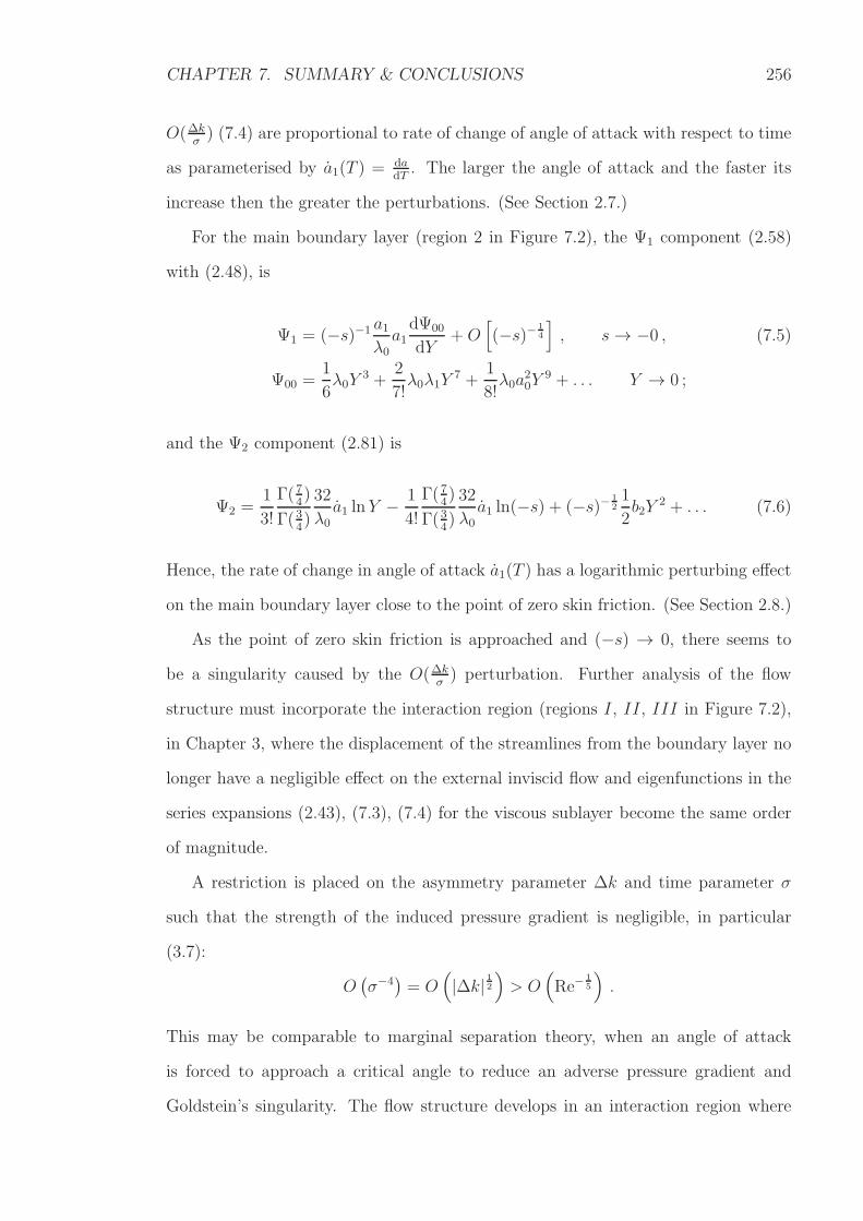
CHAPTER 7. SUMMARY & CONCLUSIONS 256
O(∆kσ) (7.4) are proportional to rate of change of angle of attack with respect to time
as parameterised by a1(T ) = dadT
. The larger the angle of attack and the faster its
increase then the greater the perturbations. (See Section 2.7.)
For the main boundary layer (region 2 in Figure 7.2), the Ψ1 component (2.58)
with (2.48), is
Ψ1 = (−s)−1 a1λ0a1
dΨ00
dY+O
[
(−s)− 14
]
, s→ −0 , (7.5)
Ψ00 =1
6λ0Y
3 +2
7!λ0λ1Y
7 +1
8!λ0a
20Y
9 + . . . Y → 0 ;
and the Ψ2 component (2.81) is
Ψ2 =1
3!
Γ(74)
Γ(34)
32
λ0a1 lnY −
1
4!
Γ(74)
Γ(34)
32
λ0a1 ln(−s) + (−s)− 1
21
2b2Y
2 + . . . (7.6)
Hence, the rate of change in angle of attack a1(T ) has a logarithmic perturbing effect
on the main boundary layer close to the point of zero skin friction. (See Section 2.8.)
As the point of zero skin friction is approached and (−s) → 0, there seems to
be a singularity caused by the O(∆kσ) perturbation. Further analysis of the flow
structure must incorporate the interaction region (regions I, II, III in Figure 7.2),
in Chapter 3, where the displacement of the streamlines from the boundary layer no
longer have a negligible effect on the external inviscid flow and eigenfunctions in the
series expansions (2.43), (7.3), (7.4) for the viscous sublayer become the same order
of magnitude.
A restriction is placed on the asymmetry parameter ∆k and time parameter σ
such that the strength of the induced pressure gradient is negligible, in particular
(3.7):
O(
σ−4)
= O(
|∆k| 12)
> O(
Re−15
)
.
This may be comparable to marginal separation theory, when an angle of attack
is forced to approach a critical angle to reduce an adverse pressure gradient and
Goldstein’s singularity. The flow structure develops in an interaction region where
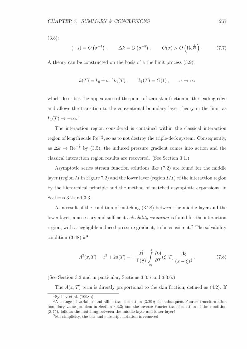
CHAPTER 7. SUMMARY & CONCLUSIONS 257
(3.8):
(−s) = O(
σ−4)
, ∆k = O(
σ−8)
, O(σ) > O(
Re120
)
. (7.7)
A theory can be constructed on the basis of a the limit process (3.9):
k(T ) = k0 + σ−8k1(T ) , k1(T ) = O(1) , σ →∞
which describes the appearance of the point of zero skin friction at the leading edge
and allows the transition to the conventional boundary layer theory in the limit as
k1(T )→ −∞.1
The interaction region considered is contained within the classical interaction
region of length scale Re−15 , so as to not destroy the triple-deck system. Consequently,
as ∆k → Re−25 by (3.5), the induced pressure gradient comes into action and the
classical interaction region results are recovered. (See Section 3.1.)
Asymptotic series stream function solutions like (7.2) are found for the middle
layer (region II in Figure 7.2) and the lower layer (region III) of the interaction region
by the hierarchical principle and the method of matched asymptotic expansions, in
Sections 3.2 and 3.3.
As a result of the condition of matching (3.28) between the middle layer and the
lower layer, a necessary and sufficient solvability condition is found for the interaction
region, with a negligible induced pressure gradient, to be consistent.2 The solvability
condition (3.48) is3
A2(x, T )− x2 + 2a(T ) = − 234
Γ(54)
x∫
−∞
∂A
∂T(ξ, T )
dξ
(x− ξ) 14
. (7.8)
(See Section 3.3 and in particular, Sections 3.3.5 and 3.3.6.)
The A(x, T ) term is directly proportional to the skin friction, defined as (4.2). If
1Sychev et al. (1998b).2A change of variables and affine transformation (3.29); the subsequent Fourier transformation
boundary value problem in Section 3.3.3; and the inverse Fourier transformation of the condition(3.45), follows the matching between the middle layer and lower layer!
3For simplicity, the bar and subscript notation is removed.
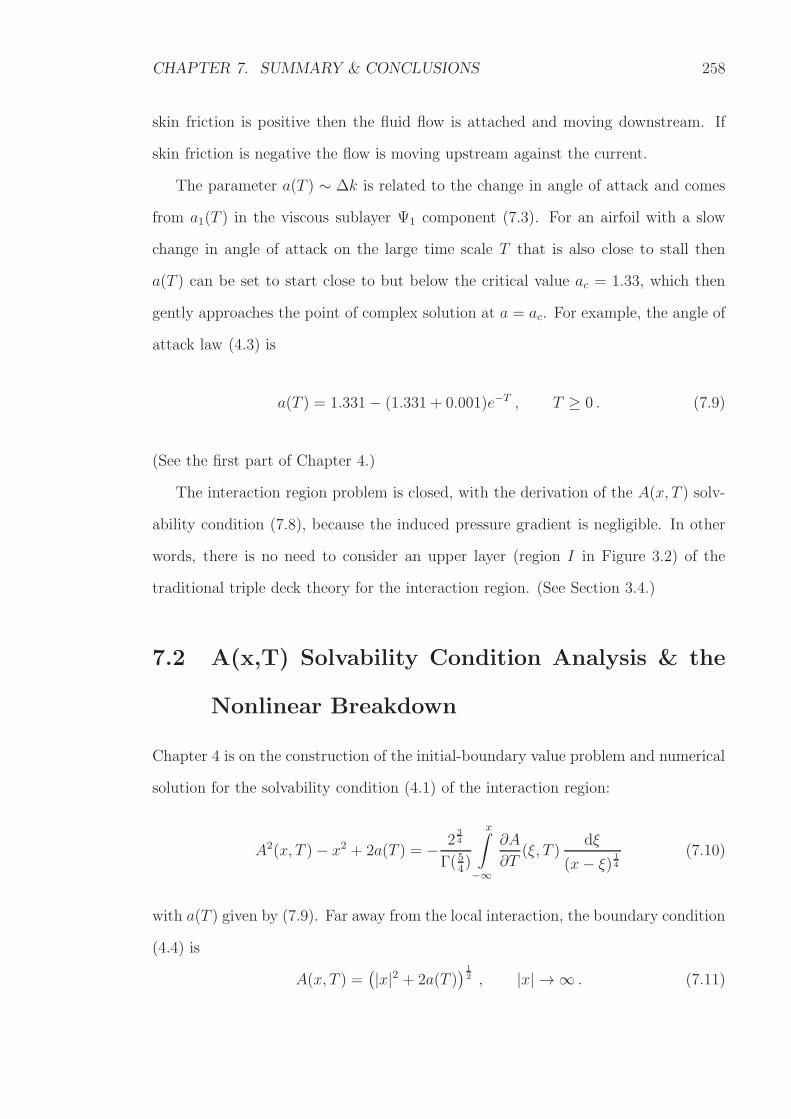
CHAPTER 7. SUMMARY & CONCLUSIONS 258
skin friction is positive then the fluid flow is attached and moving downstream. If
skin friction is negative the flow is moving upstream against the current.
The parameter a(T ) ∼ ∆k is related to the change in angle of attack and comes
from a1(T ) in the viscous sublayer Ψ1 component (7.3). For an airfoil with a slow
change in angle of attack on the large time scale T that is also close to stall then
a(T ) can be set to start close to but below the critical value ac = 1.33, which then
gently approaches the point of complex solution at a = ac. For example, the angle of
attack law (4.3) is
a(T ) = 1.331− (1.331 + 0.001)e−T , T ≥ 0 . (7.9)
(See the first part of Chapter 4.)
The interaction region problem is closed, with the derivation of the A(x, T ) solv-
ability condition (7.8), because the induced pressure gradient is negligible. In other
words, there is no need to consider an upper layer (region I in Figure 3.2) of the
traditional triple deck theory for the interaction region. (See Section 3.4.)
7.2 A(x,T) Solvability Condition Analysis & the
Nonlinear Breakdown
Chapter 4 is on the construction of the initial-boundary value problem and numerical
solution for the solvability condition (4.1) of the interaction region:
A2(x, T )− x2 + 2a(T ) = − 234
Γ(54)
x∫
−∞
∂A
∂T(ξ, T )
dξ
(x− ξ) 14
(7.10)
with a(T ) given by (7.9). Far away from the local interaction, the boundary condition
(4.4) is
A(x, T ) =(
|x|2 + 2a(T ))
12 , |x| → ∞ . (7.11)
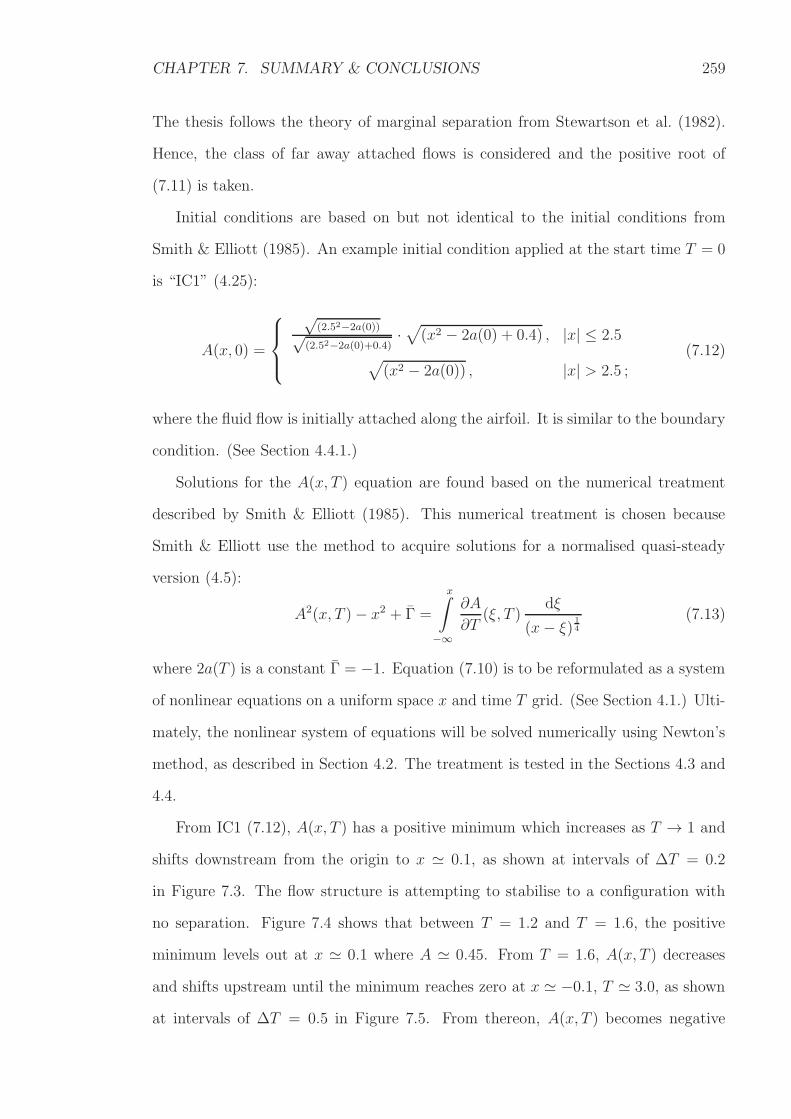
CHAPTER 7. SUMMARY & CONCLUSIONS 259
The thesis follows the theory of marginal separation from Stewartson et al. (1982).
Hence, the class of far away attached flows is considered and the positive root of
(7.11) is taken.
Initial conditions are based on but not identical to the initial conditions from
Smith & Elliott (1985). An example initial condition applied at the start time T = 0
is “IC1” (4.25):
A(x, 0) =
√(2.52−2a(0))√
(2.52−2a(0)+0.4)·√
(x2 − 2a(0) + 0.4) , |x| ≤ 2.5
√
(x2 − 2a(0)) , |x| > 2.5 ;
(7.12)
where the fluid flow is initially attached along the airfoil. It is similar to the boundary
condition. (See Section 4.4.1.)
Solutions for the A(x, T ) equation are found based on the numerical treatment
described by Smith & Elliott (1985). This numerical treatment is chosen because
Smith & Elliott use the method to acquire solutions for a normalised quasi-steady
version (4.5):
A2(x, T )− x2 + Γ =
x∫
−∞
∂A
∂T(ξ, T )
dξ
(x− ξ) 14
(7.13)
where 2a(T ) is a constant Γ = −1. Equation (7.10) is to be reformulated as a system
of nonlinear equations on a uniform space x and time T grid. (See Section 4.1.) Ulti-
mately, the nonlinear system of equations will be solved numerically using Newton’s
method, as described in Section 4.2. The treatment is tested in the Sections 4.3 and
4.4.
From IC1 (7.12), A(x, T ) has a positive minimum which increases as T → 1 and
shifts downstream from the origin to x ≃ 0.1, as shown at intervals of ∆T = 0.2
in Figure 7.3. The flow structure is attempting to stabilise to a configuration with
no separation. Figure 7.4 shows that between T = 1.2 and T = 1.6, the positive
minimum levels out at x ≃ 0.1 where A ≃ 0.45. From T = 1.6, A(x, T ) decreases
and shifts upstream until the minimum reaches zero at x ≃ −0.1, T ≃ 3.0, as shown
at intervals of ∆T = 0.5 in Figure 7.5. From thereon, A(x, T ) becomes negative
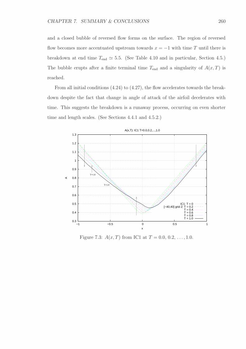
CHAPTER 7. SUMMARY & CONCLUSIONS 260
and a closed bubble of reversed flow forms on the surface. The region of reversed
flow becomes more accentuated upstream towards x = −1 with time T until there is
breakdown at end time Tend ≃ 5.5. (See Table 4.10 and in particular, Section 4.5.)
The bubble erupts after a finite terminal time Tend and a singularity of A(x, T ) is
reached.
From all initial conditions (4.24) to (4.27), the flow accelerates towards the break-
down despite the fact that change in angle of attack of the airfoil decelerates with
time. This suggests the breakdown is a runaway process, occurring on even shorter
time and length scales. (See Sections 4.4.1 and 4.5.2.)
0.3
0.4
0.5
0.6
0.7
0.8
0.9
1
1.1
1.2
1.3
−1 −0.5 0 0.5 1
A
x
A(x,T): IC1 T=0.0,0.2,...,1.0
IC1: T = 0[−40,40] grid 2: T = 0.2
T = 0.4T = 0.6T = 0.8T = 1.0
T=1.8
T=1.0
Figure 7.3: A(x, T ) from IC1 at T = 0.0, 0.2, . . . , 1.0.
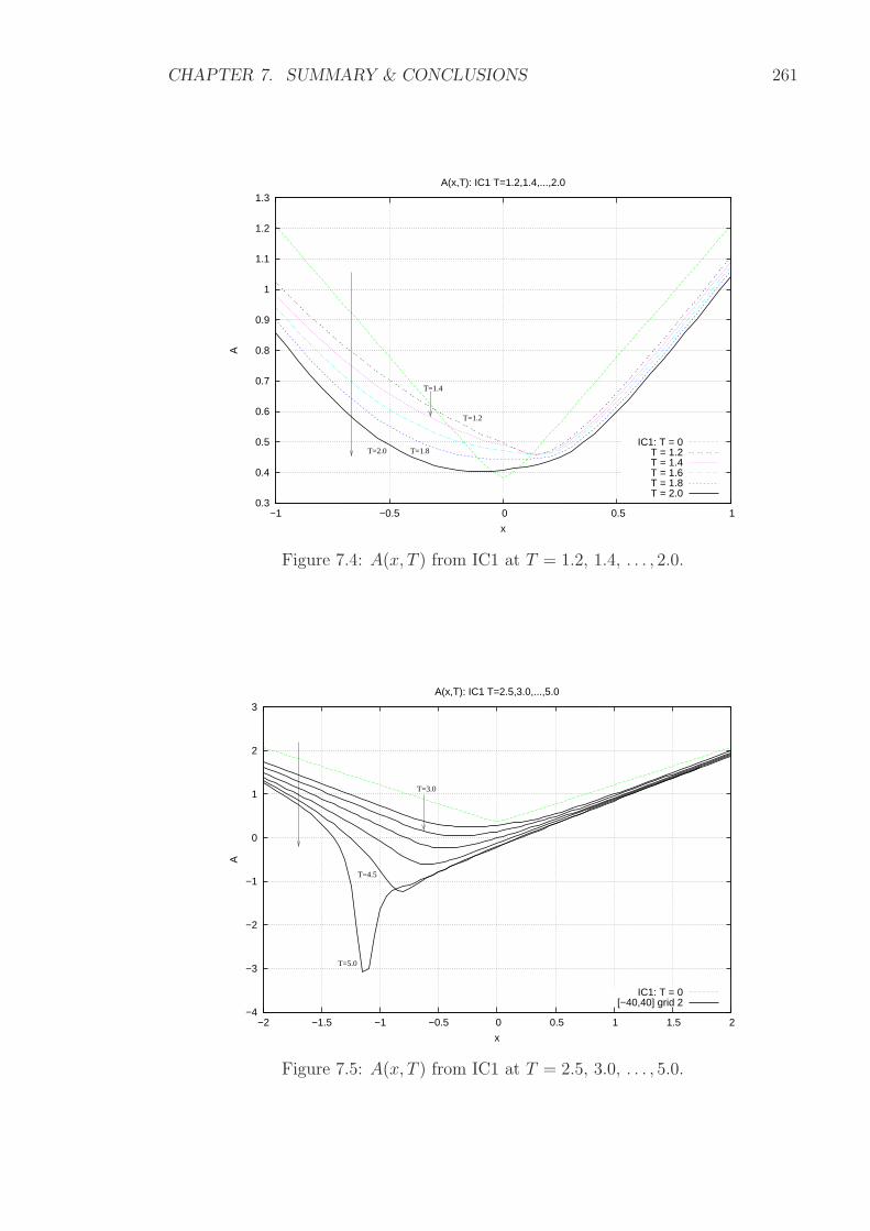
CHAPTER 7. SUMMARY & CONCLUSIONS 261
0.3
0.4
0.5
0.6
0.7
0.8
0.9
1
1.1
1.2
1.3
−1 −0.5 0 0.5 1
A
x
A(x,T): IC1 T=1.2,1.4,...,2.0
IC1: T = 0T = 1.2T = 1.4T = 1.6T = 1.8T = 2.0
T=1.2
T=1.4
T=1.8T=2.0
Figure 7.4: A(x, T ) from IC1 at T = 1.2, 1.4, . . . , 2.0.
−4
−3
−2
−1
0
1
2
3
−2 −1.5 −1 −0.5 0 0.5 1 1.5 2
A
x
A(x,T): IC1 T=2.5,3.0,...,5.0
IC1: T = 0[−40,40] grid 2
T=5.0
T=4.5
T=3.0
Figure 7.5: A(x, T ) from IC1 at T = 2.5, 3.0, . . . , 5.0.
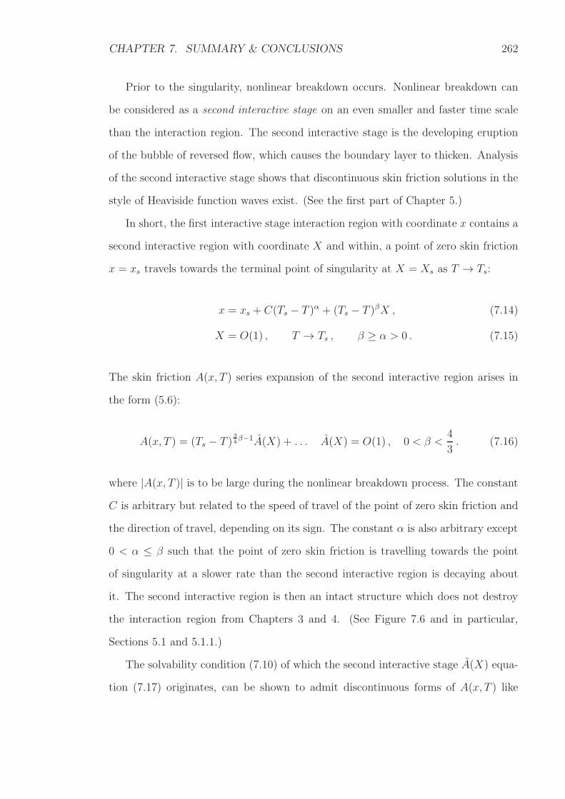
CHAPTER 7. SUMMARY & CONCLUSIONS 262
Prior to the singularity, nonlinear breakdown occurs. Nonlinear breakdown can
be considered as a second interactive stage on an even smaller and faster time scale
than the interaction region. The second interactive stage is the developing eruption
of the bubble of reversed flow, which causes the boundary layer to thicken. Analysis
of the second interactive stage shows that discontinuous skin friction solutions in the
style of Heaviside function waves exist. (See the first part of Chapter 5.)
In short, the first interactive stage interaction region with coordinate x contains a
second interactive region with coordinate X and within, a point of zero skin friction
x = xs travels towards the terminal point of singularity at X = Xs as T → Ts:
x = xs + C(Ts − T )α + (Ts − T )βX , (7.14)
X = O(1) , T → Ts , β ≥ α > 0 . (7.15)
The skin friction A(x, T ) series expansion of the second interactive region arises in
the form (5.6):
A(x, T ) = (Ts − T )34β−1A(X) + . . . A(X) = O(1) , 0 < β <
4
3. (7.16)
where |A(x, T )| is to be large during the nonlinear breakdown process. The constant
C is arbitrary but related to the speed of travel of the point of zero skin friction and
the direction of travel, depending on its sign. The constant α is also arbitrary except
0 < α ≤ β such that the point of zero skin friction is travelling towards the point
of singularity at a slower rate than the second interactive region is decaying about
it. The second interactive region is then an intact structure which does not destroy
the interaction region from Chapters 3 and 4. (See Figure 7.6 and in particular,
Sections 5.1 and 5.1.1.)
The solvability condition (7.10) of which the second interactive stage A(X) equa-
tion (7.17) originates, can be shown to admit discontinuous forms of A(x, T ) like
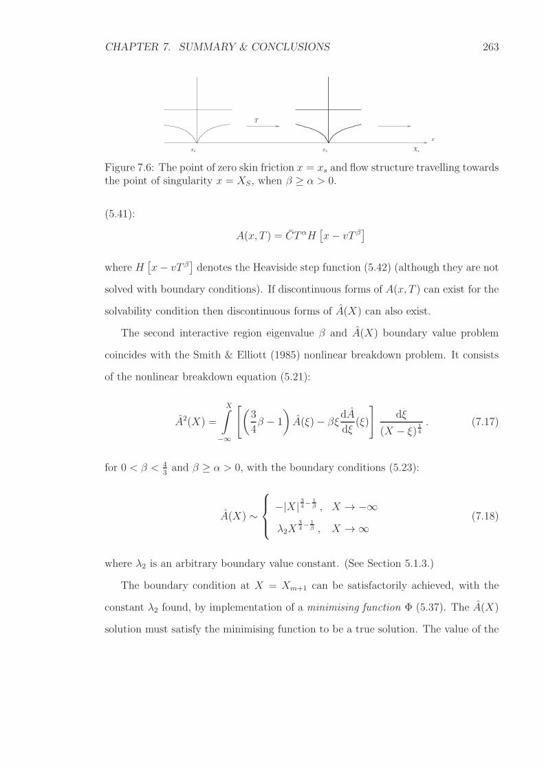
CHAPTER 7. SUMMARY & CONCLUSIONS 263
Xs
x
xs xs
T
Figure 7.6: The point of zero skin friction x = xs and flow structure travelling towardsthe point of singularity x = XS, when β ≥ α > 0.
(5.41):
A(x, T ) = CT αH[
x− vT β]
where H[
x− vT β]
denotes the Heaviside step function (5.42) (although they are not
solved with boundary conditions). If discontinuous forms of A(x, T ) can exist for the
solvability condition then discontinuous forms of A(X) can also exist.
The second interactive region eigenvalue β and A(X) boundary value problem
coincides with the Smith & Elliott (1985) nonlinear breakdown problem. It consists
of the nonlinear breakdown equation (5.21):
A2(X) =
X∫
−∞
[
(
3
4β − 1
)
A(ξ)− βξdAdξ
(ξ)
]
dξ
(X − ξ) 14
. (7.17)
for 0 < β < 43and β ≥ α > 0, with the boundary conditions (5.23):
A(X) ∼
−|X| 34− 1β , X → −∞
λ2X34− 1
β , X →∞(7.18)
where λ2 is an arbitrary boundary value constant. (See Section 5.1.3.)
The boundary condition at X = Xm+1 can be satisfactorily achieved, with the
constant λ2 found, by implementation of a minimising function Φ (5.37). The A(X)
solution must satisfy the minimising function to be a true solution. The value of the
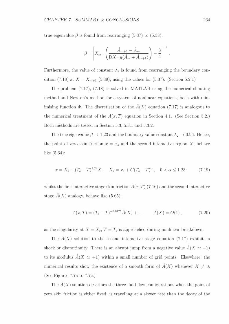
CHAPTER 7. SUMMARY & CONCLUSIONS 264
true eigenvalue β is found from rearranging (5.37) to (5.38):
β =
∣
∣
∣
∣
∣
Xm ·(
Am+1 − Am
DX · 12(Am + Am+1)
)
− 3
4
∣
∣
∣
∣
∣
−1
.
Furthermore, the value of constant λ2 is found from rearranging the boundary con-
dition (7.18) at X = Xm+1 (5.39), using the values for (5.37). (Section 5.2.1)
The problem (7.17), (7.18) is solved in MATLAB using the numerical shooting
method and Newton’s method for a system of nonlinear equations, both with min-
imising function Φ. The discretisation of the A(X) equation (7.17) is analogous to
the numerical treatment of the A(x, T ) equation in Section 4.1. (See Section 5.2.)
Both methods are tested in Section 5.3, 5.3.1 and 5.3.2.
The true eigenvalue β → 1.23 and the boundary value constant λ2 → 0.96. Hence,
the point of zero skin friction x = xs and the second interactive region X , behave
like (5.64):
x = Xs + (Ts − T )1.23X , Xs = xs + C(Ts − T )α , 0 < α ≤ 1.23 ; (7.19)
whilst the first interactive stage skin friction A(x, T ) (7.16) and the second interactive
stage A(X) analogy, behave like (5.65):
A(x, T ) = (Ts − T )−0.0775A(X) + . . . A(X) = O(1) , (7.20)
as the singularity at X = Xs, T = Ts is approached during nonlinear breakdown.
The A(X) solution to the second interactive stage equation (7.17) exhibits a
shock or discontinuity. There is an abrupt jump from a negative value A(X ≃ −1)
to its modulus A(X ≃ +1) within a small number of grid points. Elsewhere, the
numerical results show the existence of a smooth form of A(X) whenever X 6= 0.
(See Figures 7.7a to 7.7c.)
The A(X) solution describes the three fluid flow configurations when the point of
zero skin friction is either fixed; is travelling at a slower rate than the decay of the
CHAPTER 7. SUMMARY & CONCLUSIONS 265
second interactive region; or is travelling at the same rate as the decay of the second
interactive region.4 Furthermore, the flow structure is simply shifted with the point
of zero skin friction, as illustrated in Figure 7.6. (See Section 5.1.1.)
Therefore, the shock at the point of zero skin friction shows a point of detachment
or abrupt reattachment of a bubble or reversed flow to the airfoil.5 The skin friction,
being negative for X < 0, shows forward attached flow; and being positive for X > 0,
shows reversed flow in the closed bubble. The shock can either be stationary or
travelling along the airfoil towards a point of singularity. Coinciding with the decay
of the second interactive region is the increasing accentuation of the bubble which
thickens the boundary layer. Eventually, the flow regime returns to that of boundary
layer thickness, as analysed in Chapter 6. (See Section 5.4.)
4This assertion is based on Moore (1958) for moving points of separation.5Smith & Elliott (1985)
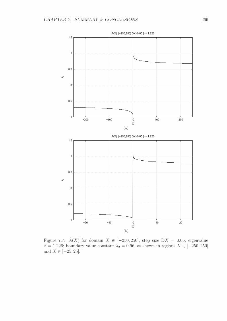
CHAPTER 7. SUMMARY & CONCLUSIONS 266
−1
−0.5
0
0.5
1
1.5
−200 −100 0 100 200
Â
X
Â(X): [−250,250] DX=0.05 β = 1.226
(a)
−1
−0.5
0
0.5
1
1.5
−20 −10 0 10 20
Â
X
Â(X): [−250,250] DX=0.05 β = 1.226
(b)
Figure 7.7: A(X) for domain X ∈ [−250, 250], step size DX = 0.05; eigenvalueβ = 1.226; boundary value constant λ2 = 0.96, as shown in regions X ∈ [−250, 250]and X ∈ [−25, 25].
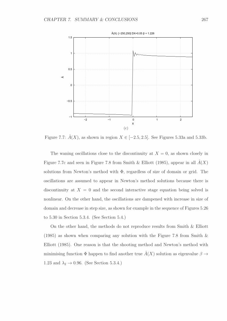
CHAPTER 7. SUMMARY & CONCLUSIONS 267
−1
−0.5
0
0.5
1
1.5
−2 −1 0 1 2
Â
X
Â(X): [−250,250] DX=0.05 β = 1.226
(c)
Figure 7.7: A(X), as shown in region X ∈ [−2.5, 2.5]. See Figures 5.33a and 5.33b.
The waning oscillations close to the discontinuity at X = 0, as shown closely in
Figure 7.7c and seen in Figure 7.8 from Smith & Elliott (1985), appear in all A(X)
solutions from Newton’s method with Φ, regardless of size of domain or grid. The
oscillations are assumed to appear in Newton’s method solutions because there is
discontinuity at X = 0 and the second interactive stage equation being solved is
nonlinear. On the other hand, the oscillations are dampened with increase in size of
domain and decrease in step size, as shown for example in the sequence of Figures 5.26
to 5.30 in Section 5.3.4. (See Section 5.4.)
On the other hand, the methods do not reproduce results from Smith & Elliott
(1985) as shown when comparing any solution with the Figure 7.8 from Smith &
Elliott (1985). One reason is that the shooting method and Newton’s method with
minimising function Φ happen to find another true A(X) solution as eigenvalue β →
1.23 and λ2 → 0.96. (See Section 5.3.4.)
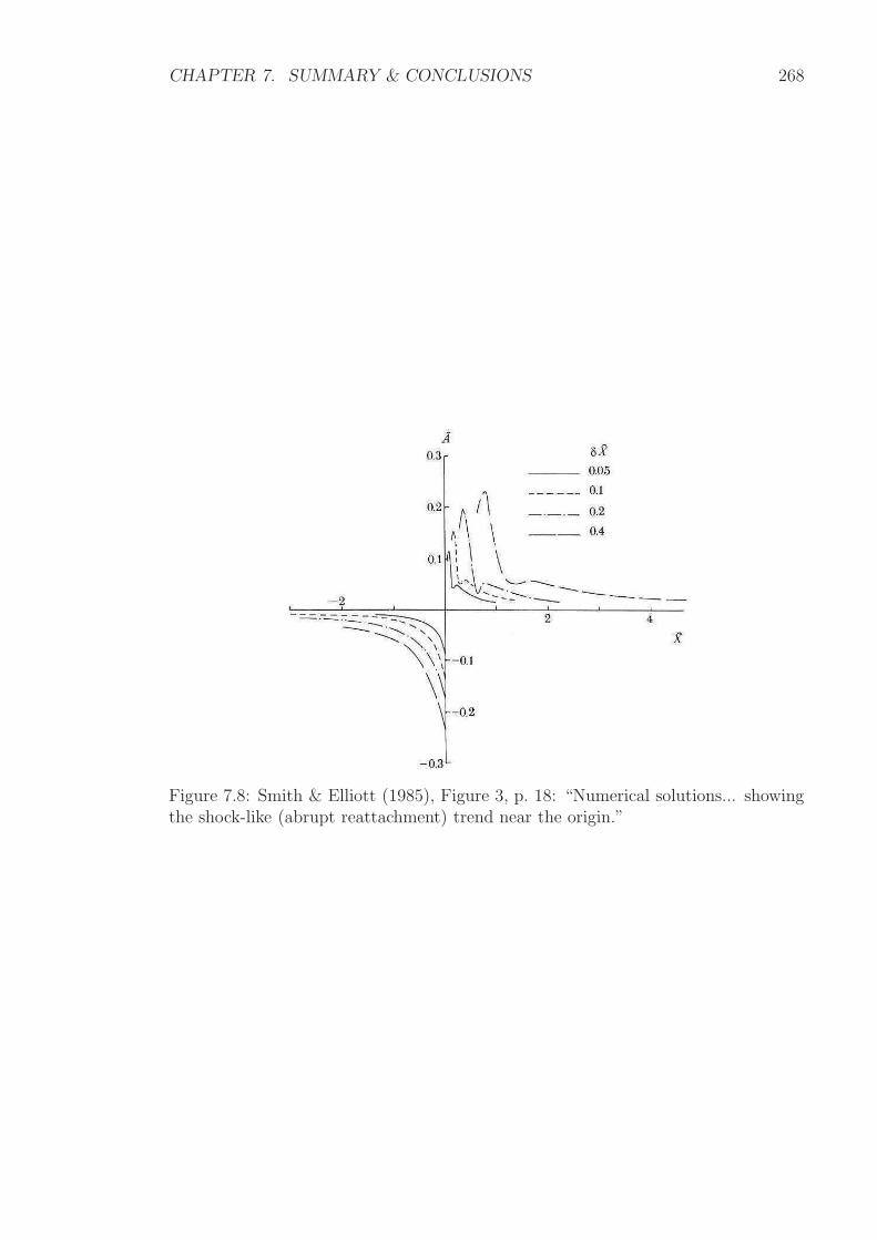
CHAPTER 7. SUMMARY & CONCLUSIONS 268
Figure 7.8: Smith & Elliott (1985), Figure 3, p. 18: “Numerical solutions... showingthe shock-like (abrupt reattachment) trend near the origin.”
CHAPTER 7. SUMMARY & CONCLUSIONS 269
7.3 Leading Edge Stall & Inviscid Euler Structure
The process of leading edge stall continues from the second interactive stage nonlinear
breakdown (Chapter 5), where there is runaway growth of a bubble of reversed flow
and discontinuous skin friction advancing towards a singularity. The induced pressure
gradient (Section 3.1), that was made negligible in the interaction region by the slow
perturbations to the airfoil on a large time scale T , exists in the unsteady interactive
structure, regardless of the time scale on which the structure exists. Ultimately, the
flow regime is that where time and length scales shorten to the scale of boundary
layer thickness. The flow reaches a nonlinear Euler stage where the growth of the
bubble spans the boundary layer. Evidence for the terminal flow is from analysis of
the leading edge, starting with the boundary layer and its governing equations. The
analysis follows from that of dynamic stall due to unsteady marginal separation by
Elliott & Smith (1987), which has been adapted in Chapter 6.
According to the analysis, the terminal Euler flow regime is a short-scale break-
down with |X− X0| ∼ |T − T0|35 , and with the viscous flow splitting into two.6 There
is an external inviscid part which erupts like Y ∼ |T − T0|−15 and a diminishing inner
viscous region with Y ∼ |T − T0|−12 . Eventually the external region will be indistin-
guishable from the majority of the boundary layer of thickness O(Re−12 ). This occurs
when the Eulerian scalings:
t− σT − Re−17 T0 = O
(
Re−12
)
(7.21)
x− xs − Re15x∗ − Re−
27 X0 = O
(
Re−12
)
are true. The velocity and pressure disturbances become increased to order unity
and so the Euler equations come into operation across the entire boundary layer. A
vortex starts to span the boundary layer and its evolution becomes a vortex sheet
problem. (See Section 6.4.)
6See also Elliott & Smith (1987).
CHAPTER 7. SUMMARY & CONCLUSIONS 270
The effects described in Chapter 6 mark the end of the second interactive stage of
the thickening of the boundary layer and the start of a third interactive stage where
there is unsteady vortex development and ejection. The third interactive stage is the
process of leading edge stall.
7.4 Further Work
Firstly, some further calculations need to be done to confirm error contributions from
the integral (4.8) with the limits minus infinity to x1 in the numerical treatment
of the solvability condition A(x, T ) equation in Section 4.1 and from the analogous
integral (5.25) with limits minus infinity to X1 the second interactive stage nonlinear
breakdown A(X) equation in Section 5.2.
The error contributions are found from the solution of the integrals with the next
order terms of the integrands. The integral (4.8) for the A(x, T ) equation uses the
derivative with respect to time T of the boundary condition (4.4):
A(x, T ) =(
|x|2 + 2a(T ))
12 , |x| → ∞
as part of the integrand. The boundary condition itself is derived from (4.4):
A2(x, T ) = |x|2 + 2a(T ) +a2(T )
|x|2 + . . . |x| → ∞
and hence, the next order term of the integrand involves the third term on the right
hand side. The integral (5.25) for the A(X) equation also involves the boundary
condition (5.23):
A(X) ∼ −|X| 34− 1β , X → −∞ ;
however, its next order terms are not considered in the thesis and requires more work.
The original aim of the thesis was to bridge work on marginal separation with
that steady flow over a downstream-moving surface, unsteady marginal separation
CHAPTER 7. SUMMARY & CONCLUSIONS 271
and dynamic stall. Slow perturbations from a slow change in angle of attack on a
very large time scale are applied to the airfoil so as to weaken the induced pressure
gradient in the interaction region. The slow perturbations can be applied to any airfoil
problem mentioned in Recent Works (Chapter 1), for example, three-dimensional
marginal separation theory, flows over obstacles, local suction flows, flows with severe
pressure gradients or abruptly-started airfoils.
Bibliography
Abramovich, M. and Stegun, I. A. (1972). Handbook of Mathematical Functions with
Formulas, Graphs, and Mathematical Tables, National Bureau of Standards, 9
edn, Wiley-Interscience.
Anderson, Jr, J. D. (1997). The History of Aerodynamics and its Impact on Flying
Machines, Cambridge University Press.
Anderson, Jr, J. D. (2008). Introduction to Flight, 6 edn, New York: McGraw-Hill
Higher Education.
Atkinson, K. and Han, W. (2003). Elementary Numerical Analysis, 3 edn, Wiley.
Batchelor, G. K. (2000a). An Introduction to Fluid Dynamics, Cambridge University
Press, chapter 4.
Batchelor, G. K. (2000b). An Introduction to Fluid Dynamics, Cambridge University
Press, chapter 6.
Batchelor, G. K. (2000c). An Introduction to Fluid Dynamics, Cambridge University
Press, chapter 3.
Blasius, H. (1908). Grenzschichten in flussigkeiten mit kleiner reibung., Z. Math.
Phys. 56(1): 1–37. English translation NACA TM 1256.
Braun, S. (2006). Recent developments in the asymptotic theory of separated
flows. levenshulme lectures - lecture notes., Manchester Institute of Mathematics
EPrints 2006.226. http://eprints.ma.man.ac.uk/656/.
272
BIBLIOGRAPHY 273
Braun, S. and Kluwick, A. (2002). The effect of three-dimensional obstacles on
marginally separated laminar boundary layer flows., Journal of Fluid Mechanics
406: 57–82.
Braun, S. and Kluwick, A. (2004). Unsteady three-dimensional marginal separa-
tion caused by surface-mounted obstacles and/or local suction., Journal of Fluid
Mechanics 514: 121–152.
Braun, S. and Kluwick, A. (2005). Blow-up and control of marginally separated
boundary layer flows., 363: 1057–1067.
Brown, S. N. (1965). Singularities associated with separating boundary layers., Philo-
sophical Transactions of the Royal Society London A 257: 409–444.
Brown, S. N. and Stewartson, K. (1969). Laminar separation., Annual Review of
Fluid Mechanics 1: 45–79.
Brown, S. N. and Stewartson, K. (1983). On an integral equation of marginal sepa-
ration., SIAM Journal of Applied Mathematics 43(5): 1119–1126.
Cassel, K. W. (2000). A comparison of navier-stokes solutions with the theoreti-
cal description of unsteady separation., Philosophical Transactions of the Royal
Society London A 358: 3207–3227.
Cassel, K. W. and Obabko, A. V. (2010). A rayleigh instability in vortex-induced
unsteady boundary layer., Physica Scripta T142: 1–14.
Cassel, K. W., Smith, F. T. and Walker, J. D. A. (1996). The onset of stability in
unsteady boundary-layer separation., Journal of Fluid Mechanics 315: 223–256.
Catherall, D. and Mangler, K. W. (1966). The integration of the two-dimensional lam-
inar boundary-layer equations past the point of vanishing skin friction., Journal
of Fluid Mechanics 26(1): 163–182.
BIBLIOGRAPHY 274
Chernyshenko, S. I. (1985). On the asymptotics of stationary solutions of the
navier-stokes equations at large reynolds numbers., Dokl. Akad. Nauk SSSR
285(6): 1353–1355. English translation.
Crabtree, L. F. (1959). The formation of regions of separated flow on wing sur-
faces. part i. low-speed tests on a two-dimensional unswept wing with a 10 per
cent thick rae 101 section., Reports and Memoranda, Part I 3122, Aeronautical
Research Council.
Degani, A. T., Li, Q. and Walker, J. D. A. (1996). Unsteady separation from the
leading edge of a thin airfoil., Physics of Fluids 8(3): 489–512.
Duck, P. W. (1990). Unsteady three-dimensional marginal separation including break-
down., Journal of Fluid Mechanics 220: 85–98.
Elliott, J. W. and Smith, F. T. (1987). Dynamic stall due to unsteady marginal
separation., Journal of Fluid Mechanics 179: 489–512.
Elliott, J. W., Smith, F. T. and Cowley, S. J. (1983). Breakdown of boundary layers:
(i) on moving surfaces; (ii) in semi-similar unsteady flow; (iii) in fully unsteady
flow., Geophysical and Astrophysical Fluid Dynamics 25: 77–138.
Goldstein, S. (1930). Concerning some solutions of the boundary layer equations in
hydrodynamics., Proceedings of the Cambridge Philosophical Society 26(1): 1–30.
Goldstein, S. (1948). On laminar boundary-layer flow near a position of separation.,
Quarterly Journal of Mechanics and Applied Mathematics 1(1): 43–69.
Gorenflo, R. and Vessella, S. (2008). Abel Integral Equations: Analysis and Applica-
tions, Lecture Notes In Mathematics, Springer-Verlag New York.
Hackmuller, G. and Kluwick, A. (1990a). Effects of surface geometry and suc-
tion/blowing on marginal separation., in A. H. Nayfeh and A. Mobarak (eds),
Proc. 3rd Intl Congre. of Fluid Mechanics, Cairo, Vol. 1, Cairo University, pp. 1–
6.
BIBLIOGRAPHY 275
Hackmuller, G. and Kluwick, A. (1990b). Effects of three-dimensional surface
mounted obstacles on marginal separation., in V. V. Kozlov and A. V. Dov-
gal (eds), Separated Flows and Jets, Springer, pp. 55–65.
Hartree, D. R. (1939). A solution of the laminar boundary-layer equation for retarded
flow., A. R. C. R. & M. 2426.
Howarth, L. (1938). On the solution of the laminar boundary layer equations., Pro-
ceedings of the Royal Society, London, A 164: 547–579.
Jones, B. M. (1933). An experimental study of the stalling of wings., A. R. C. R. &
M. 1588.
Jones, B. M. (1934). Stalling., Journal of the Royal Aeronautical Society 38: 753–770.
Koromilas, C. A. and Telionis, D. P. (1980). Unsteady laminar separation: an exper-
imental study., Journal of Fluid Mechanics 97(2): 347–384.
Kuryanov, A. I., Stolyarov, G. I. and Steinberg, R. I. (1979). On the hysteresis of
aerodynamic characteristics., Uch. Zap. TsAGI 10(3): 12–15. in Russian.
Landau, L. D. and Lifshitz, E. M. (1944). Mechanics of Continuous Media, Gostekhiz-
dat Moscow. English translation.
Lighthill, M. J. (1951). A new approach to thin airfoil theory., Aeronautical Quarterly
3(3): 193–210.
Lighthill, M. J. (1953). On boundary layers and upstream influence. i. a compar-
ison between subsonic and supersonic flows., Proceedings of the Royal Society,
London, A 217: 344–357.
Lighthill, M. J. (1958). On displacement thickness., Journal of Fluid Mechanics
4(4): 383–392.
Lighthill, M. J. (1963). Introduction: Boundary layer theory, in L. Rosenhead (ed.),
Laminar Boundary Layers, Oxford University Press, chapter 2.
BIBLIOGRAPHY 276
McCroskey, W. J. (1982). Annual review of unsteady airfoils, Fluid Mechanics
14: 285–311.
Messiter, A. F. (1979). Boundary-layer separation., Proc. 8th U.S. Natl. Congr. Appl.
Mech. pp. 157–179. Western Periodicals, North Hollywood, CA.
Messiter, A. F. (1983). Boundary-layer interaction theory., ASME Journal of Applied
Mechanics 50(4b): 1104–1115.
Messiter, A. F. and Enlow, R. L. (1973). A model for laminar boundary-layer flow
near a separation point., SIAM Journal of Applied Mathematics 25(3): 655–670.
Moore, F. K. (1958). On the separation of the unsteady boundary layer., in H. Gortler
(ed.), Boundary Layer Research, Springer Berlin, pp. 296–311.
Muskhelishvili, N. I. (1953). Singular Integral Equations: Boundary problems of
function theory and their application to mathematical physics., 2 edn, Groningen:
P. Noordhoff. Translation from the Russian edited by J. R. M. Radok.
Neiland, V. Y. (1969). Theory of laminar boundary-layer separation in supersonic
flow., Fluid Dynamics 4(4): 33–35. English translation.
Obabko, A. V. and Cassel, K. W. (2002a). Detachment of the dynamic stall above a
moving surface., AIAA Journal 40(9): 1811–1822.
Obabko, A. V. and Cassel, K. W. (2002b). Navier-stokes solutions of unsteady sep-
aration induced by a vortex., Journal of Fluid Mechanics 465: 99–130.
Obabko, A. V. and Cassel, K. W. (2005). On the ejection induced instability in
navier-stokes solutions of unsteady separation., Philosophical Transactions of
the Royal Society London A 363: 1189–1198.
Prandtl, L. (1904). Motion of fluids with very little viscosity., NACA Technical
Memorandum 452. English translation.
BIBLIOGRAPHY 277
Prandtl, L. (1935). The mechanics of viscous fluids, in W. F. Durand (ed.), Aerody-
namic Theory, Vol. 3, Springer Berlin, pp. 34–208.
Rosenhead, L. (1963). Laminar Boundary Layers, Calrendon Press, Oxford, chap-
ter 3.
Rott, N. (1956). Unsteady viscous flow in the vicinity of a stagnation point., The
Quarterly Journal of Mechanics and Applied Mathematics 13: 444–451.
Ruban, A. I. (1981). Singular solution of boundary layer equations which can be
extended continuously through the point of zero surface friction., Fluid Dynamics
16(6): 835–843.
Ruban, A. I. (1982a). Asymptotic theory of short separation regions on the leading
edge of a slender airfoil., Fluid Dynamics 17(1): 33–41.
Ruban, A. I. (1982b). Stability of preseparation boundary layer on the leading edge
of a thin airfoil., Fluid Dynamics 17(6): 860–867. English translation.
Ryzhov, O. S. and Smith, F. T. (1984). Short-length instabilities, breakdown and
initial value problems in dynamic stall., Mathematika: a Journal of Pure and
Applied Mathematics 31(2): 163–177.
Samad, M. A. (2004). Three Dimensional Marginal Separation Theory, PhD thesis,
University of Manchester, School of Mathematics.
Scheichl, S., Braun, S. and Kluwick, A. (2008). On a similarity solution in the theory
of unsteady marginal separation., Acta Mechanica 201: 153–170.
Sears, W. R. (1956). Some recent developments in airfoil theory., Journal of Aero-
nautical Sciences 23(5): 490–499.
Sears, W. R. and Telionis, D. P. (1971). Unsteady boundary layer separation., in
E. Eichelbrenner (ed.), Recent Research on Unsteady Boundary Layers, Vol. 1 of
Proc. Symposium of I. U. T. A. M., Laval University Press, Quebec, pp. 404–407.
BIBLIOGRAPHY 278
Sears, W. R. and Telionis, D. P. (1975). Boundary-layer separation in unsteady flow.,
SIAM Journal of Applied Mathematics 28(1): 215–235.
Smith, F. T. (1982a). Concerning dynamic stall., Aeronautical Quarterly 33(4): 331–
352.
Smith, F. T. (1982b). On the high reynolds number theory of laminar flows., IMA
Journal of Applied Mathematics 28: 207–281.
Smith, F. T. and Daniels, P. G. (1981). Removal of goldstein’s singularity at separa-
tion, in flow past obstacles in wall layers., Journal of Fluid Mechanics 110: 1–37.
Smith, F. T. and Elliott, J. W. (1985). On the abrupt reattachment downstream
of leading-edge laminar separation., Proceedings of the Royal Society, London A
401(1820): 1–27.
Stavrou, S. (2004). Boundary Layer Separation Control and Receptivity Aspects in
Marginal Separation Theory., PhD thesis, University of Manchester, School of
Mathematics.
Stewartson, K. (1958). On goldstein’s theory of laminar separation., Quarterly Jour-
nal of Mechanics and Applied Mathematics 11(4): 391–410.
Stewartson, K. (1960). The theory of unsteady laminar boundary layers., Advances
in Applied Mechanics 6, Academic Press, New York, pp. 1–37.
Stewartson, K. (1970). Is the singularity at separation removable?, Journal of Fluid
Mechanics 44(2): 347–364.
Stewartson, K., Smith, F. T. and Kaups, K. (1982). Marginal separation., Studies in
Applied Mathematics 67(1): 45–61.
Stewartson, K. and Williams, P. G. (1969). Self-induced separation., Proceedings of
the Royal Society, London A 312: 181–206.
BIBLIOGRAPHY 279
Suli, E. and Mayers, D. (2003). An Introduction to Numerical Analysis, Cambridge
University Press.
Sychev, V. V. (1972). Laminar separation., Fluid Dynamics 7(3): 407–417. English
translation.
Sychev, V. V., Ruban, A. I., Sychev, V. V. and Korolev, G. L. (1998a). Asymptotic
Theory of Separated Flows, Cambridge University Press, chapter 1.
Sychev, V. V., Ruban, A. I., Sychev, V. V. and Korolev, G. L. (1998b). Asymptotic
Theory of Separated Flows, Cambridge University Press, chapter 4.
Sychev, V. V., Ruban, A. I., Sychev, V. V. and Korolev, G. L. (1998c). Asymptotic
Theory of Separated Flows, Cambridge University Press, chapter 5.
Sychev, V. V., Ruban, A. I., Sychev, V. V. and Korolev, G. L. (1998d). Asymptotic
Theory of Separated Flows, Cambridge University Press, chapter 2.
Tani, I. (1964). Low speed flows involving bubble separations., Progress in Aerospace
Sciences 5: 70–103.
Telionis, D. P. and Werle, M. J. (1973). Boundary layer separation from downstream-
moving boundaries., Journal of Applied Mechanics 40(2): 369–374.
van Dyke, M. D. (1956). Second-order subsonic airfoil theory including edge effects.,
NACA Technical Memorandum 1274.
van Dyke, M. D. (1975). Perturbation Methods in Fluid Mechanics, Parabolic Press.
Werle, M. J. and Davis, R. T. (1972). Incompressible laminar boundary layers on a
parabola at an angle of attack: a study of the separation point., ASME Journal
Of Applied Mechanics 39(1): 7–12.
White, F. M. (2006). Viscous Fluid Flow, 3 edn, McGraw-Hill.
Appendix A
Derivation of the Navier-Stokes
Equations
The Navier-Stokes equations are named after Claude-Louis Navier and George Gabriel
Stokes who first derived the equations in the nineteenth century in accordance with
the continuum hypothesis of fluids, Newton’s Second Law and the principles of con-
servation of mass, momentum and energy.1
The fluid is assumed to be Newtonian in the thesis. The fluid motion is subsonic
and within the framework of the traditional two-dimensional Cartesian coordinate
system (x, y) with time t. Hence, the equations are described in this system also.
Newton’s Second Law, when applied to a solid body is written as
ma = f
for the mass of the body m, acceleration a and the force applied to the body f ,
such as gravity. When Newton’s Second Law is formulated for fluid dynamics, the
momentum equation
ρDv
Dt= ρf +∇ ·Σ (A.1)
holds for density ρ, velocity vector of the fluid v = (u, v) with tangential and normal
1See White (2006) and Batchelor (2000c) for more detailed derivations.
280
APPENDIX A. DERIVATION OF THE NAVIER-STOKES EQUATIONS 281
velocity components u and v; body force f ; and surface force stress tensor Σ. The
material derivative is defined as
D
Dt=
∂
∂t+ u
∂
∂x+ v
∂
∂y.
The divergence of stress tensor Σ is
(∇ ·Σ)i =∂Σji
∂xj, i = 1, 2 (A.2)
in traditional tensor notation.2 3
The principles of conservation require that the sum of changes of a property such
as mass, momentum or energy over a controlled volume must be equal to what is
gained or lost through the boundaries of the volume plus what is created or destroyed
by sources or sinks respectively inside the volume. The conservation of mass density
ρ can be written as:
∂ρ
∂t+∇ · (ρv) = 0
and in an incompressible fluid where ρ is a constant quantity, then
∇ · v =∂u
∂x+∂v
∂y= 0 . (A.3)
2Equation (A.2) can be written as
(∇ ·Σ)i =
2∑
j=1
∂Σji
∂xj
, i = 1, 2
where indices i, j = 1, 2 are representative of the components of the two-dimensional Cartesiancoordinate system x, y respectively. For i = 1:
(∇ ·Σ)x =∂Σxx
∂x+
∂Σyx
∂y
and for i = 2:
(∇ ·Σ)y =∂Σxy
∂x+
∂Σyy
∂y
3The component Σji is the stress on the j-th plane in the i-th direction. For example, for i, j = 1both corresponding to the x coordinate then Σxx is the stress on the x-plane of an infinitesimal(cuboid) volume of fluid in the direction parallel to the x-axis.
APPENDIX A. DERIVATION OF THE NAVIER-STOKES EQUATIONS 282
A consequence of (A.3) for a Newtonian fluid is that the body forces and stress tensors
are related by the constitutive equation:
Σji = −pδji + µ
(
∂vj∂xi
+∂vi∂xj
)
(A.4)
for pressure p, constant dynamic viscosity µ and the Kronecker delta δji:
δji =
1 , j = i
0 , j 6= i .
The combination of Newton’s Second Law (A.1), stress tensor (A.2), mass conser-
vation law (A.3) and the constitutive equation (A.4) gives the Navier-Stokes equations
for incompressible, Newtonian fluids (in coordinate decomposition):
∂u
∂t+ u
∂u
∂x+ v
∂u
∂y= fx −
1
ρ
∂p
∂x+ ν
(
∂2u
∂x2+∂2u
∂y2
)
,
∂v
∂t+ u
∂v
∂x+ v
∂v
∂y= fy −
1
ρ
∂p
∂y+ ν
(
∂2v
∂x2+∂2v
∂y2
)
,
∂u
∂x+∂v
∂y= 0 ,
with constant kinetic viscosity ν = µ
ρ.
Appendix B
The Integral of Small Perturbation
Theory
The subsonic pressure-displacement relation (3.50) or (6.34) is obtained from the
integral of small perturbation theory. The integral can be sought by considering the
theory of separation from a smooth surface, adapted from Sychev, Ruban, Sychev
and Korolev (1998a).
The independent variables and the stream function solutions for the boundary
layer and interaction region in high Reynolds number flow across a smooth surface
are found using the hierarchical process, similar to that for the boundary layer and
interaction region in Chapters 2 and 3. The independent variables of the lower layer
(region III) of the interaction region are
x∗ = Re38x = O(1) , Y ∗ = Re
58 y = Re
18Y = O(1)
where x, Y are the classical boundary layer coordinates and y is the normal coor-
dinate of the external inviscid region. The displacement effect of the lower layer
from flow over a smooth surface is transmitted across the middle layer (region II) of
the interaction region without change, by (3.17). The angle of inclination θ of the
283
APPENDIX B. THE INTEGRAL OF SMALL PERTURBATION THEORY 284
displaced streamlines is defined by the asymptotic expression:
θ = Re−14G (x∗) + . . . , G (x∗) = lim
Y ∗→∞
−∂Ψ∗0
∂x∗/∂Ψ∗
0
∂Y ∗
. (B.1)
The flow of the upper layer (region I) of the interaction region is determined
by the method of small perturbations. From the order of magnitude of θ (B.1), a
solution is sought in the form:
u = 1 + Re−14u1 (x
∗, y∗) + . . . , v = Re−14 v1 (x
∗, y∗) + . . . ,
p = p00 + Re−14p1 (x
∗, y∗) + . . .
The independent variables of the upper layer are
x∗ = Re38x , y∗ = Re
38y . (B.2)
If the longitudinal and transverse scales are not the same, degenerate equations are
formed. The Navier-Stokes equations become a system of linearised Euler equations:
∂u1∂x∗
+∂p1∂x∗
= 0 ,∂v1∂x∗
+∂p1∂y∗
= 0 ,∂u1∂x∗
+∂v1∂y∗
= 0 . (B.3)
The streamline solutions must satisfy the Brillouin-Villat condition of smooth sep-
aration to define a unique solution and hence, the upper layer flow solution must
match to the curvature of the free streamline:
κ = −kx− 12 + κ0 +O(x
12 ) , x→ +0
where k is related to the point of zero skin friction and separation. The pressure
gradient along the body surface is:
dpedx
= k(−x)− 12 +
16
3k2 +O
[
(−x) 12
]
, x→ −0 ,
APPENDIX B. THE INTEGRAL OF SMALL PERTURBATION THEORY 285
dpedx
= 0 , x > 0 .
The solution is obtained using the classical small-disturbance theory by introducing
the analytic function:
w(z) = p1 + iv1
of the complex variable z = x∗+ iy∗. The analytic function can be represented in the
form:
w(z) = Φ(z) + i2c1z12 .
The condition of matching with that of the main external inviscid flow (region 1) as
|z| → ∞, is
Φ→ 0 , |z| → ∞ .
On the real axis:
ℑΦ|y∗=0 = −2c1x∗12H (x∗) +G (x∗) ,
where H (x∗) is the Heaviside function. The analytic function Φ(z) in the upper
half-plane under the matching conditions has the form:
Φ(z) =1
π−∞∫
−∞
G(t)− 2c1t12H(t)
(t− z) dt . (B.4)
Using the Plemelj-Sokhotsky formula1 and separating the real and imaginary parts,
the pressure distribution is given (without the bookwork) as:
p1 (x∗, 0) = P ∗
0 (x∗) = −2c1 |x∗|
12 H (−x∗) + 1
π−∞∫
−∞
G(t)− 2c1t12H(t)
(t− x∗) dt . (B.5)
1The Plemelj-Sokhotsky formulae are used to solve singular integral equations, as shown inMuskhelishvili (1953).
APPENDIX B. THE INTEGRAL OF SMALL PERTURBATION THEORY 286
Therefore, the formula for the pressure gradient has the form:
∂p1∂x∗
∣
∣
∣
∣
y∗=0
=dP ∗
0
dx∗=
1
π−∞∫
−∞
G′(t)
(t− x∗) dt . (B.6)
This is the integral of small-perturbation theory.