Embed Size (px)
Citation preview
Learning 0
Learning !! !Basic principles !
Suggested reading:!
• Chapter 8 in Dayan, P. & Abbott, L., Theoretical Neuroscience, MIT Press, 2001.!
Learning 1
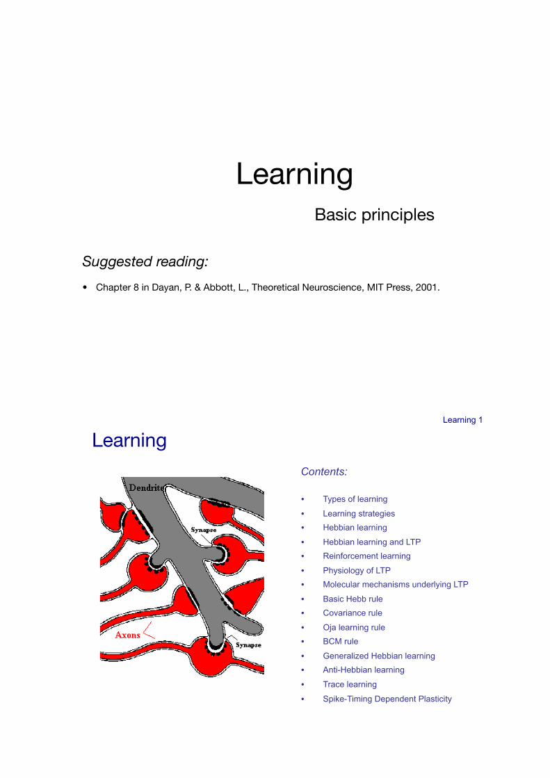
Contents:
• Was is lerning?
• Zellulärer Mechanismus der LTP • Unüberwachtes Lernen
• Überwachtes Lernen • Delta-Lernregel
• Fehlerfunktion • Gradientenabstiegsverfahren
• Reinforcement Lernen
Learning!
Contents:
• Types of learning
• Learning strategies • Hebbian learning
• Hebbian learning and LTP • Reinforcement learning
• Physiology of LTP • Molecular mechanisms underlying LTP
• Basic Hebb rule • Covariance rule
• Oja learning rule • BCM rule
• Generalized Hebbian learning • Anti-Hebbian learning
• Trace learning
• Spike-Timing Dependent Plasticity
Learning 2
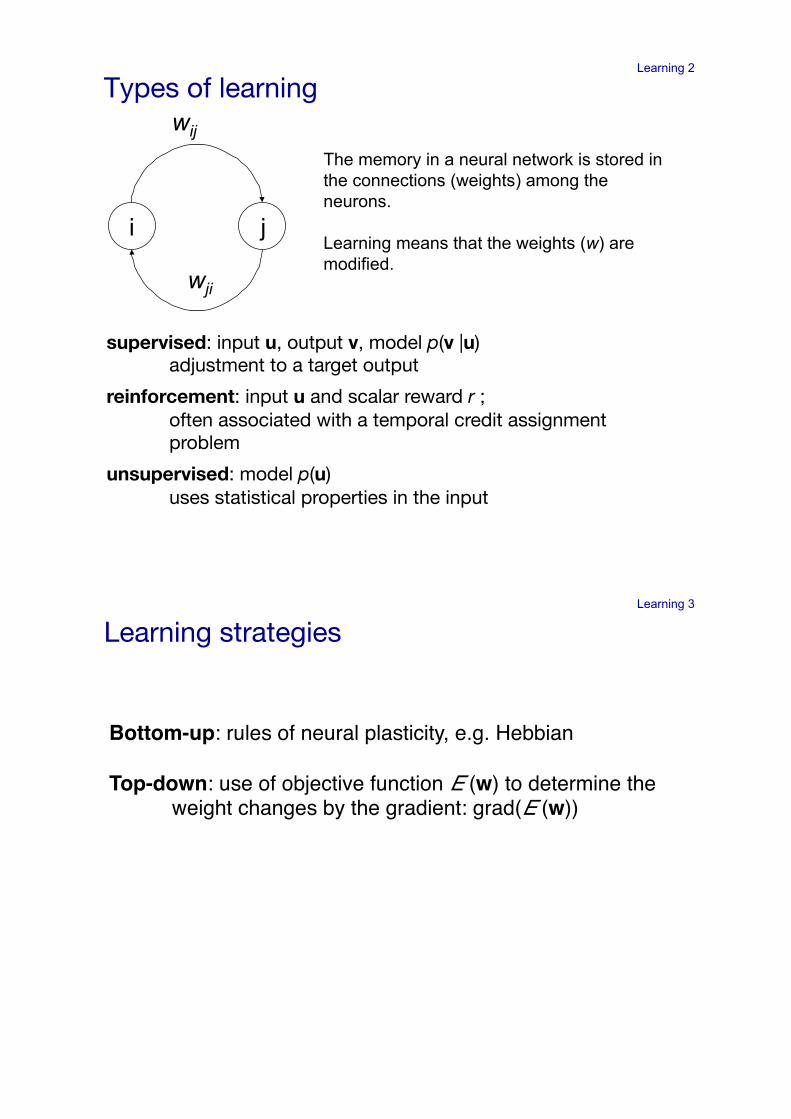
The memory in a neural network is stored in the connections (weights) among the neurons.
Learning means that the weights (w) are modified.
j i
wij
wji
supervised: input u, output v, model p(v |u) !!adjustment to a target output!
reinforcement: input u and scalar reward r ; !!often associated with a temporal credit assignment !!problem !
unsupervised: model p(u)!!uses statistical properties in the input!
Types of learning!
Learning 3
Bottom-up: rules of neural plasticity, e.g. Hebbian "
Top-down: use of objective function E (w) to determine the "weight changes by the gradient: grad(E (w)) "
Learning strategies!
Learning 4
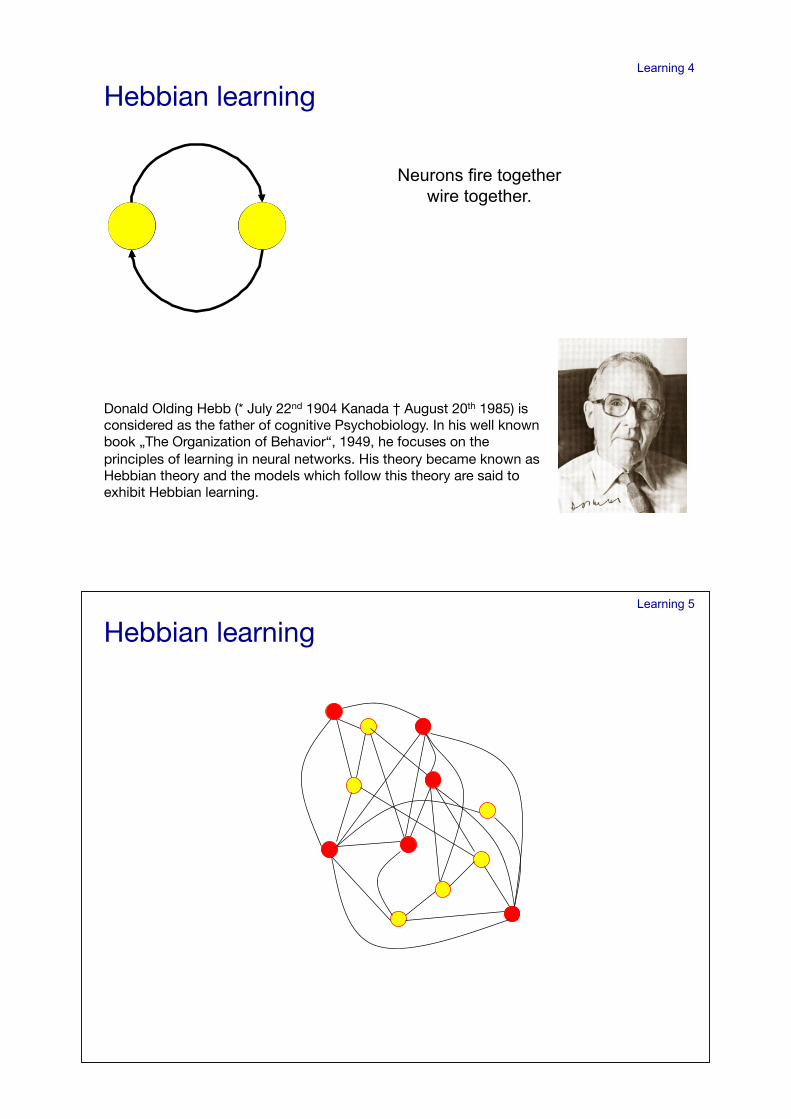
Donald Olding Hebb (* July 22nd 1904 Kanada † August 20th 1985) is considered as the father of cognitive Psychobiology. In his well known book „The Organization of Behavior“, 1949, he focuses on the principles of learning in neural networks. His theory became known as Hebbian theory and the models which follow this theory are said to exhibit Hebbian learning."
Neurons that fire together!wire together!
Hebbian learning!
Neurons fire together wire together.
Learning 5
Hebbian learning!
Learning 6
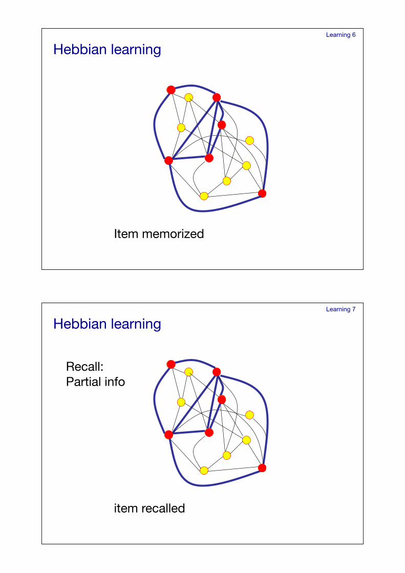
Item memorized!
Hebbian learning!
Learning 7
item recalled!
Recall:!Partial info!
Hebbian learning!
Learning 8
pre j
post i
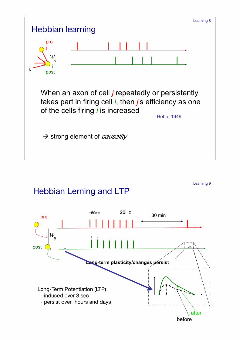
When an axon of cell j repeatedly or persistently takes part in firing cell i, then j’s efficiency as one of the cells firing i is increased
Hebb, 1949
k
Hebbian learning!
! strong element of causality "
Learning 9
pre j
post i
Long-Term Potentiation (LTP) ! - induced over 3 sec! - persist over hours and days!
+50ms 20Hz
Long-term plasticity/changes persist
30 min
before after
Hebbian Lerning and LTP!
Learning 10
pre post
i j
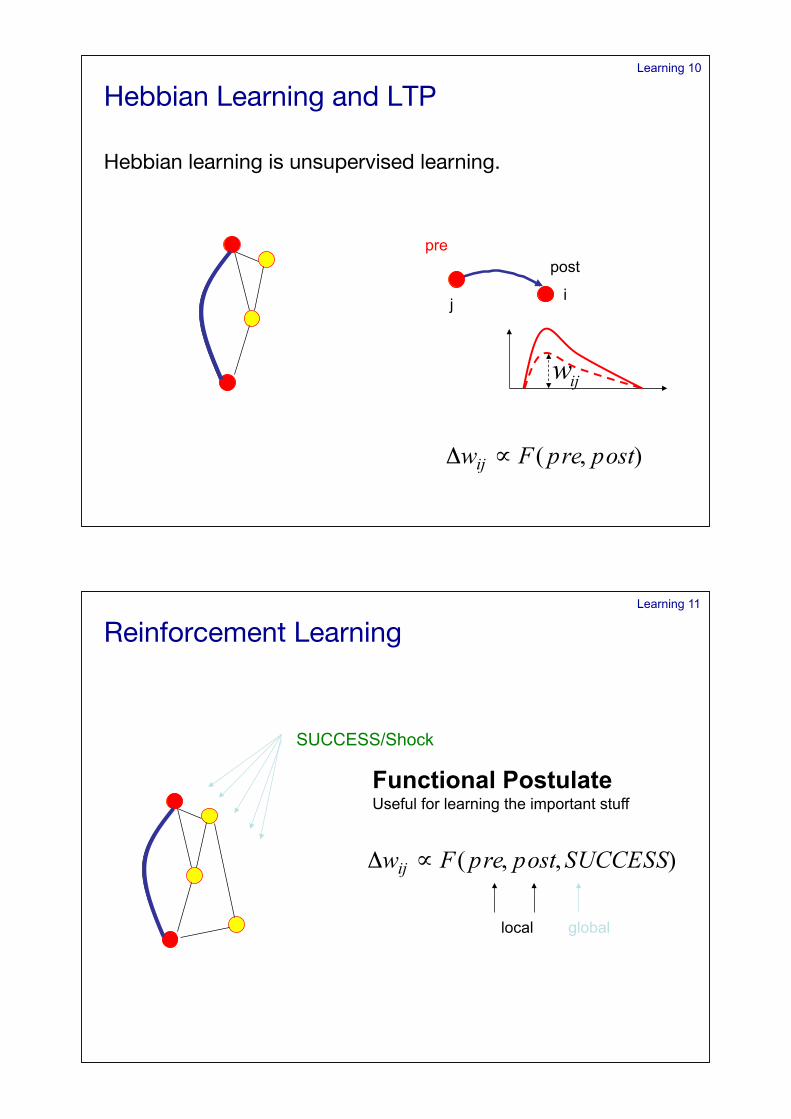
Hebbian Learning and LTP!
Hebbian learning is unsupervised learning.!
Learning 11
SUCCESS/Shock
local global
Functional Postulate Useful for learning the important stuff
Reinforcement Learning!
Learning 12
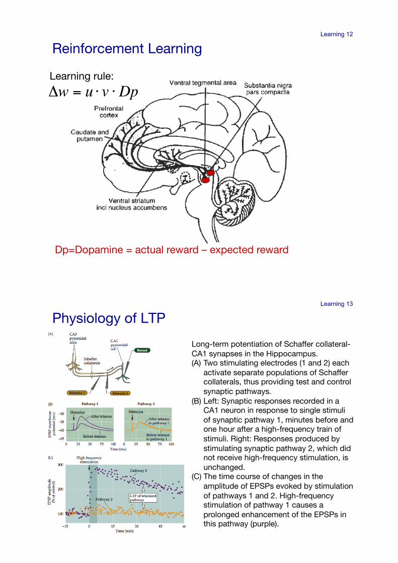
Dp=Dopamine = actual reward – expected reward!
Learning rule:!
!
"w = u # v #Dp
Reinforcement Learning!Reinforcement Learning!
Learning 13
Long-term potentiation of Schaffer collateral-CA1 synapses in the Hippocampus. !(A) Two stimulating electrodes (1 and 2) each
activate separate populations of Schaffer collaterals, thus providing test and control synaptic pathways. !
(B) Left: Synaptic responses recorded in a CA1 neuron in response to single stimuli of synaptic pathway 1, minutes before and one hour after a high-frequency train of stimuli. Right: Responses produced by stimulating synaptic pathway 2, which did not receive high-frequency stimulation, is unchanged.!
(C) The time course of changes in the amplitude of EPSPs evoked by stimulation of pathways 1 and 2. High-frequency stimulation of pathway 1 causes a prolonged enhancement of the EPSPs in this pathway (purple).!
Physiology of LTP!
Learning 14
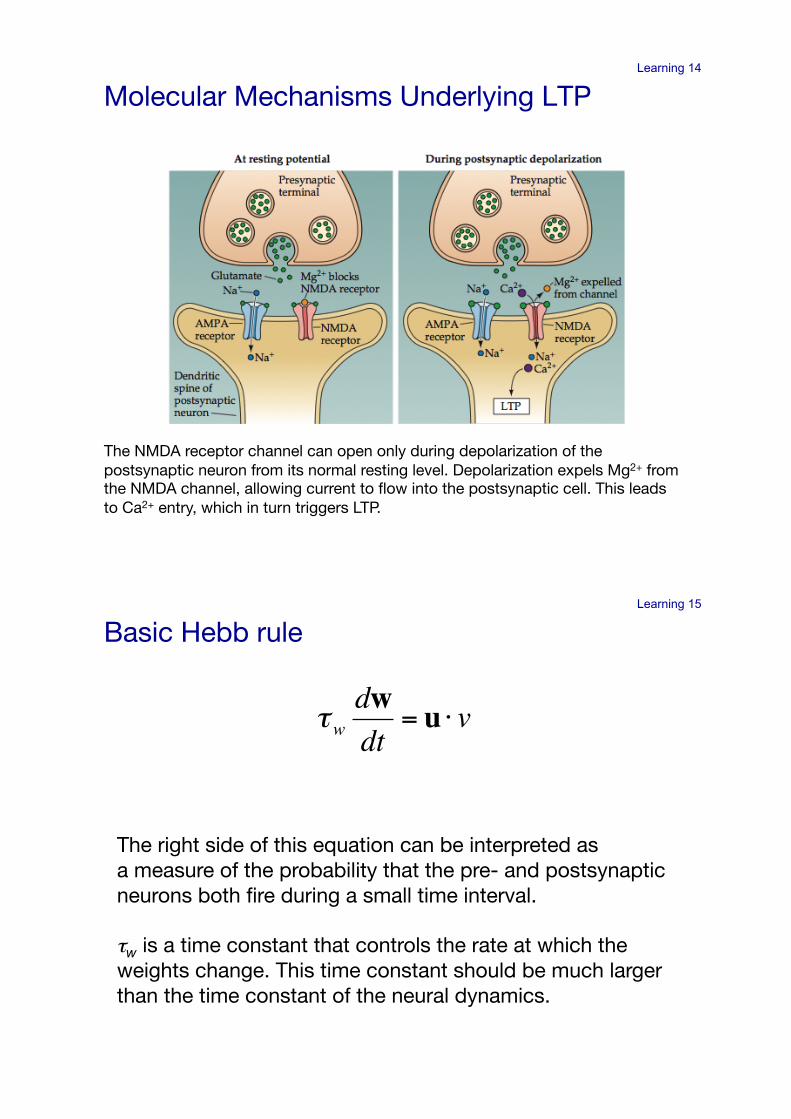
Molecular Mechanisms Underlying LTP !
The NMDA receptor channel can open only during depolarization of the postsynaptic neuron from its normal resting level. Depolarization expels Mg2+ from the NMDA channel, allowing current to flow into the postsynaptic cell. This leads to Ca2+ entry, which in turn triggers LTP.!
Learning 15
The right side of this equation can be interpreted as!a measure of the probability that the pre- and postsynaptic neurons both fire during a small time interval. !
!w is a time constant that controls the rate at which the weights change. This time constant should be much larger than the time constant of the neural dynamics.!
!
"wdwdt
= u # v
Basic Hebb rule!
Learning 16
!
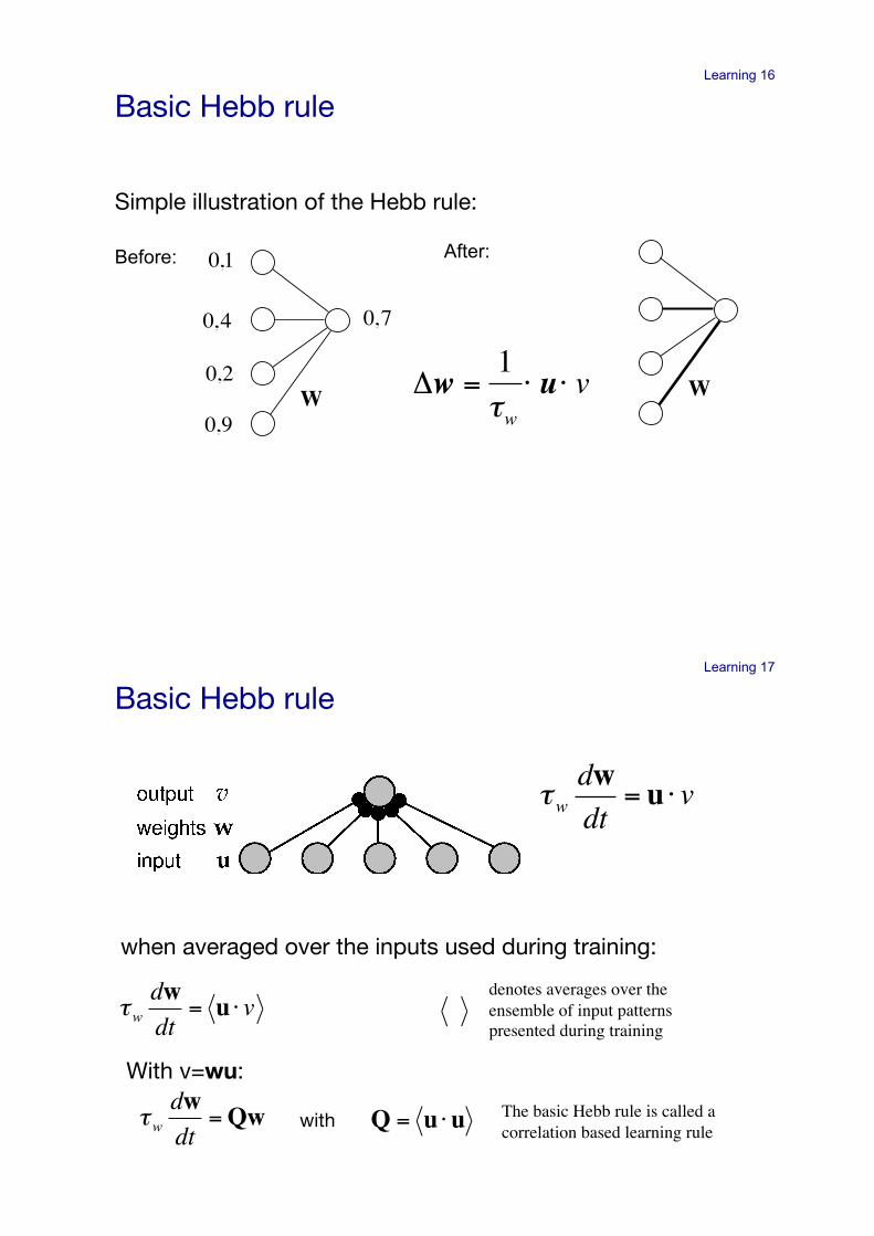
"w =1#w$ u$ v
!
W
!
0,9 !
0,7
!
0,2
!
0,4!
0,1
!
W
After: Before:
Basic Hebb rule!
Simple illustration of the Hebb rule:!
Learning 17
!
"wdwdt
= u # v
when averaged over the inputs used during training: !
!
"wdwdt
= u # v
!
denotes averages over the ensemble of input patterns presented during training!
With v=wu: !
!
"wdwdt
=Qw
!
Q = u "uwith! The basic Hebb rule is called a correlation based learning rule!
Basic Hebb rule!
Learning 18
!
"wdwdt
= v #$v( )u
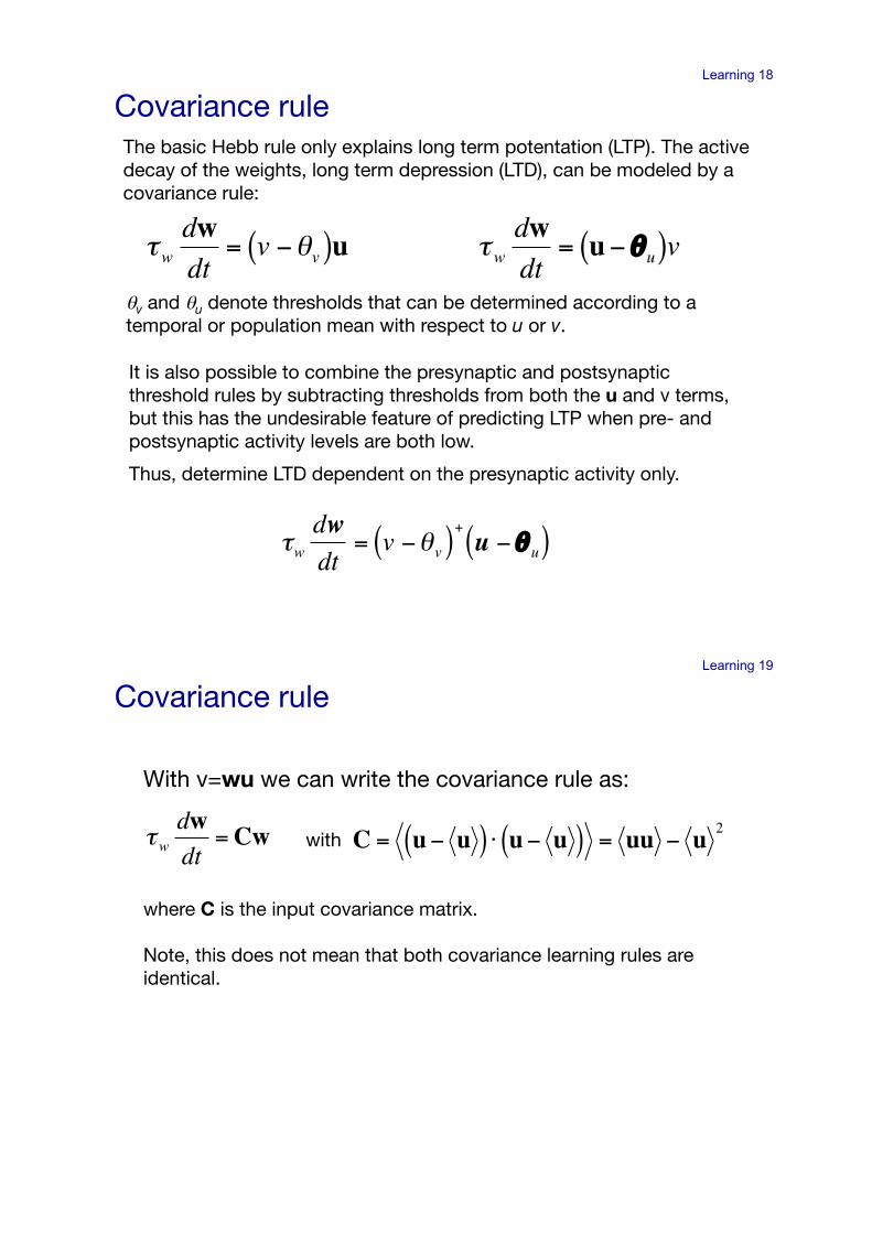
It is also possible to combine the presynaptic and postsynaptic threshold rules by subtracting thresholds from both the u and v terms, but this has the undesirable feature of predicting LTP when pre- and postsynaptic activity levels are both low.!
Thus, determine LTD dependent on the presynaptic activity only.!
The basic Hebb rule only explains long term potentation (LTP). The active decay of the weights, long term depression (LTD), can be modeled by a covariance rule:!
!
"wdwdt
= u#$u( )v
!
"wdwdt
= v #$v( )+u #$ u( )
"v and "u denote thresholds that can be determined according to a temporal or population mean with respect to u or v.!
Covariance rule!
Learning 19
where C is the input covariance matrix. !
Note, this does not mean that both covariance learning rules are identical.!
With v=wu we can write the covariance rule as:!
!
"wdwdt
=Cw
!
C = u" u( ) # u" u( ) = uu " u 2with!
Covariance rule!
Learning 20
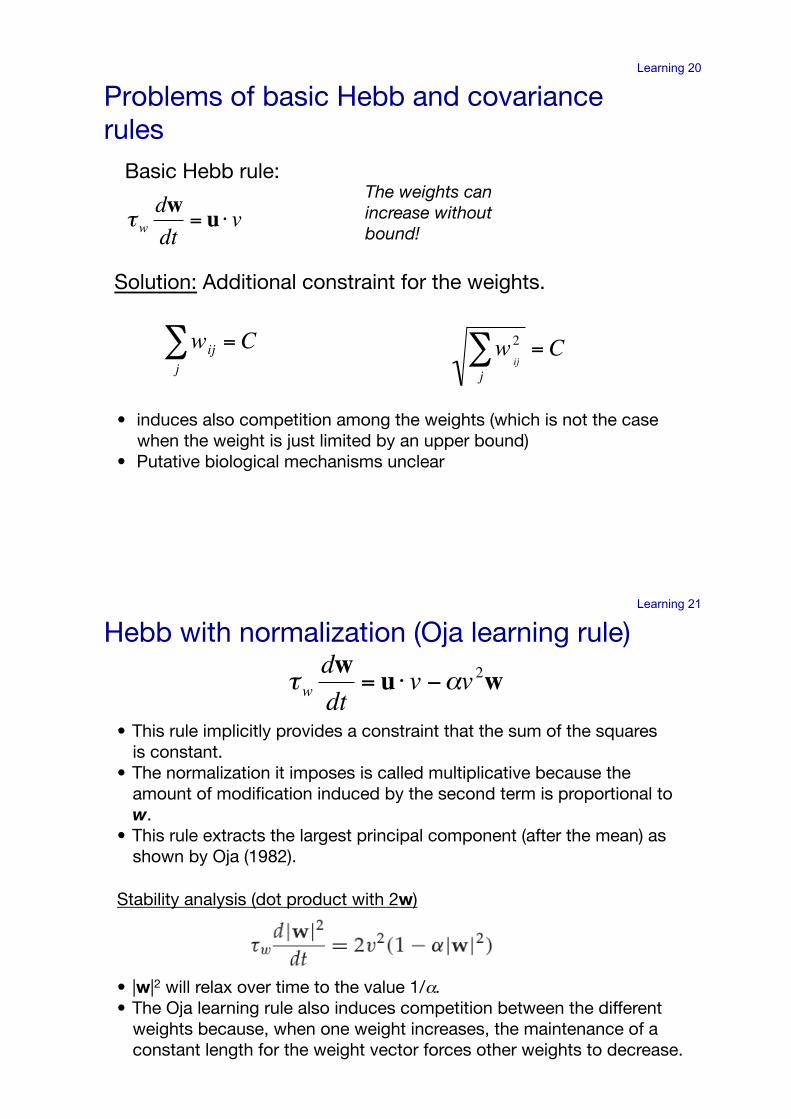
Solution: Additional constraint for the weights.!
!
wij = Cj"
!
wij
2
j" = C
• induces also competition among the weights (which is not the case when the weight is just limited by an upper bound)!
• Putative biological mechanisms unclear!
!
"wdwdt
= u # vThe weights can increase without bound!!
Basic Hebb rule:!
Problems of basic Hebb and covariance rules!
Learning 21
• This rule implicitly provides a constraint that the sum of the squares is constant. !
• The normalization it imposes is called multiplicative because the amount of modification induced by the second term is proportional to w.!
• This rule extracts the largest principal component (after the mean) as shown by Oja (1982).!
!
"wdwdt
= u # v $%v 2w
• |w|2 will relax over time to the value 1/#.!• The Oja learning rule also induces competition between the different
weights because, when one weight increases, the maintenance of a constant length for the weight vector forces other weights to decrease.!
Stability analysis (dot product with 2w)!
Hebb with normalization (Oja learning rule)!
Learning 22
!
"wdwdt
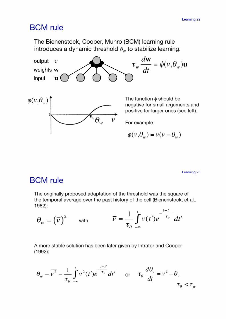
= #(v,$w )u
The Bienenstock, Cooper, Munro (BCM) learning rule introduces a dynamic threshold "w to stabilize learning. !
The function ! should be negative for small arguments and positive for larger ones (see left).!
For example:!
!
"(v,#w ) = v(v $#w )!
"(v,#w )
!
"w
!
v
BCM rule!
Learning 23
The originally proposed adaptation of the threshold was the square of the temporal average over the past history of the cell (Bienenstock, et al., 1982):!
!
"w = v ( )2 with!
!
v = 1"#
v(t$)e%
t% t '"#
%&
t
' dt$
A more stable solution has been later given by Intrator and Cooper (1992):!
!
"w = v 2 =1#"
v 2(t$)e%t% t $#"
%&
t
' dt$ or!
!
"#d#vdt
= v 2 $#v
!
"# < "w
BCM rule!
Learning 24
!
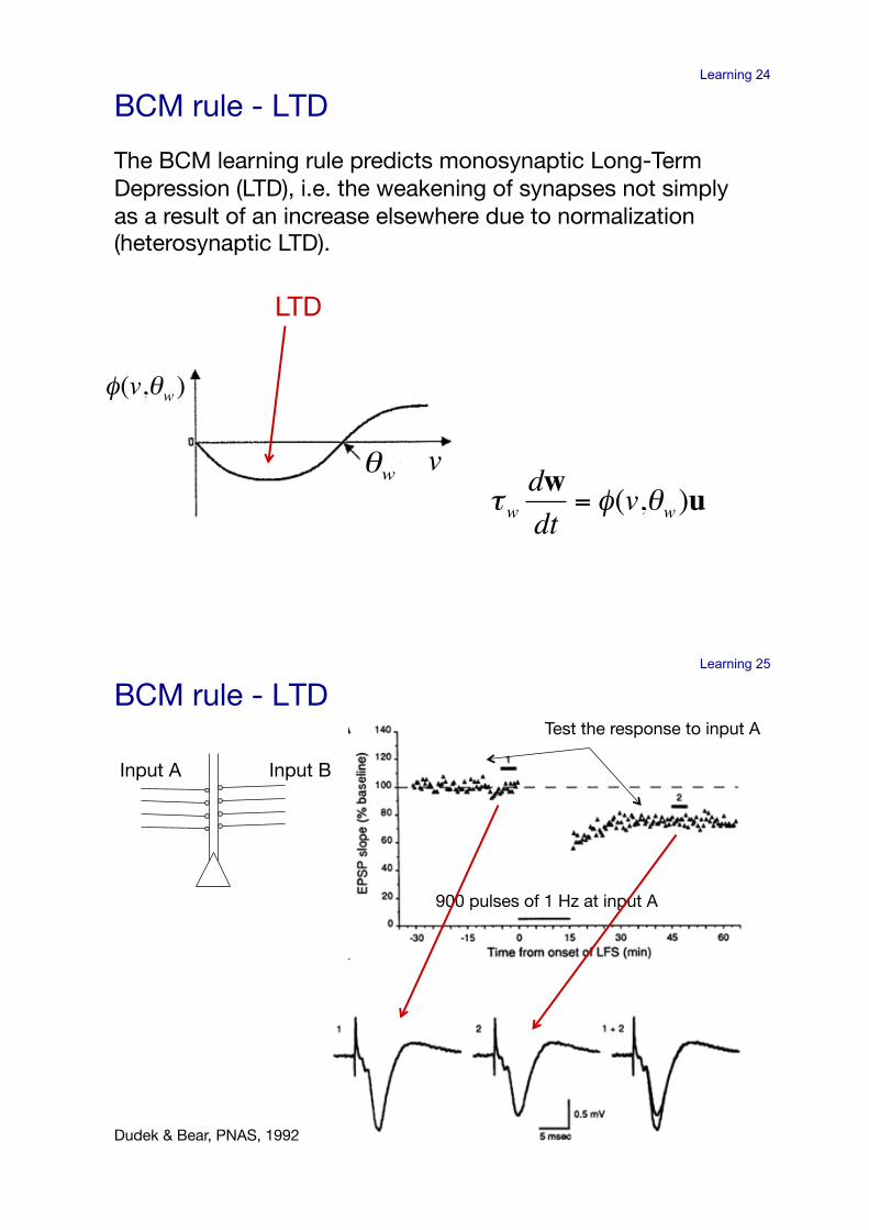
"wdwdt
= #(v,$w )u
The BCM learning rule predicts monosynaptic Long-Term Depression (LTD), i.e. the weakening of synapses not simply as a result of an increase elsewhere due to normalization (heterosynaptic LTD). !
!
"(v,#w )
!
"w
!
v
BCM rule - LTD!
LTD!
Learning 25
BCM rule - LTD!
Input A! Input B!
900 pulses of 1 Hz at input A!
Test the response to input A!
Dudek & Bear, PNAS, 1992!
Learning 26
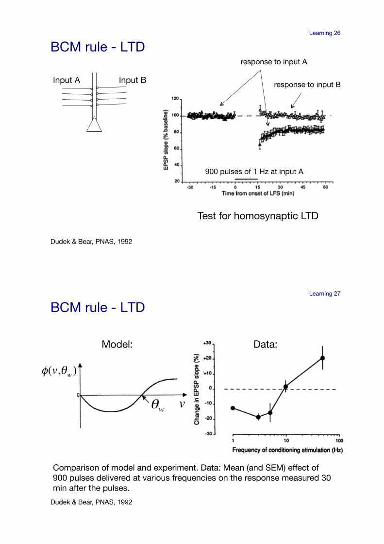
BCM rule - LTD!
Input A! Input B!
response to input A!
Dudek & Bear, PNAS, 1992!
900 pulses of 1 Hz at input A!
response to input B!
Test for homosynaptic LTD!
Learning 27
BCM rule - LTD!
Dudek & Bear, PNAS, 1992!
Comparison of model and experiment. Data: Mean (and SEM) effect of 900 pulses delivered at various frequencies on the response measured 30 min after the pulses.!
!
"(v,#w )
!
"w
!
v
Model:! Data:!
Learning 28
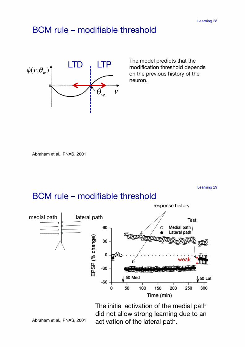
BCM rule – modifiable threshold!
Abraham et al., PNAS, 2001!
The model predicts that the modification threshold depends on the previous history of the neuron.!
!
"(v,#w )
!
"w
!
v
LTP!LTD!
Learning 29
BCM rule – modifiable threshold!
medial path!
response history!
Test!
The initial activation of the medial path did not allow strong learning due to an activation of the lateral path.!Abraham et al., PNAS, 2001!
weak!
lateral path!
Learning 30
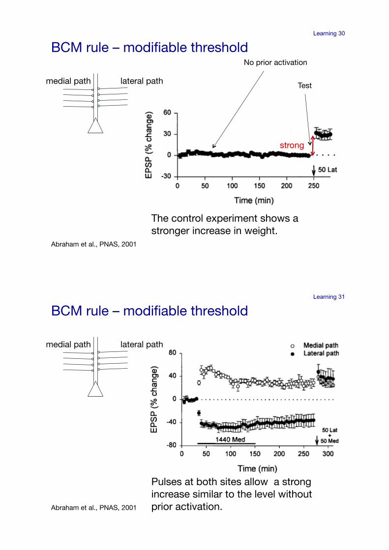
BCM rule – modifiable threshold!
medial path! lateral path!
No prior activation!
Test!
The control experiment shows a stronger increase in weight.!
Abraham et al., PNAS, 2001!
strong!
Learning 31
BCM rule – modifiable threshold!
medial path! lateral path!
Pulses at both sites allow a strong increase similar to the level without prior activation.!Abraham et al., PNAS, 2001!
Learning 32
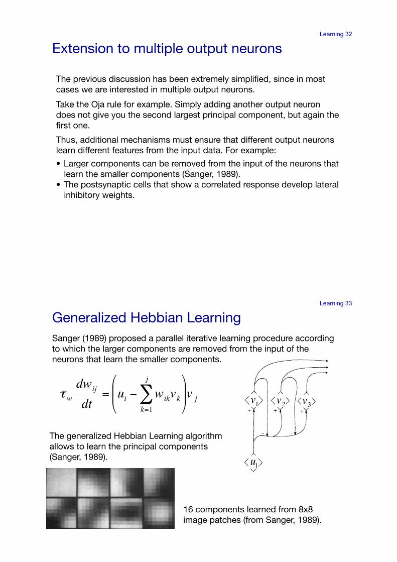
The previous discussion has been extremely simplified, since in most cases we are interested in multiple output neurons.!
Take the Oja rule for example. Simply adding another output neuron does not give you the second largest principal component, but again the first one.!
Thus, additional mechanisms must ensure that different output neurons learn different features from the input data. For example: !
• Larger components can be removed from the input of the neurons that learn the smaller components (Sanger, 1989).!
• The postsynaptic cells that show a correlated response develop lateral inhibitory weights.!
Extension to multiple output neurons!
Learning 33
Sanger (1989) proposed a parallel iterative learning procedure according to which the larger components are removed from the input of the neurons that learn the smaller components.!
!
"wdwij
dt= ui # wik
k=1
j
$ vk%
& '
(
) * v j
!
u1!
v3
!
v2
!
v1
The generalized Hebbian Learning algorithm allows to learn the principal components (Sanger, 1989).!
16 components learned from 8x8 image patches (from Sanger, 1989).!
Generalized Hebbian Learning!
Learning 34
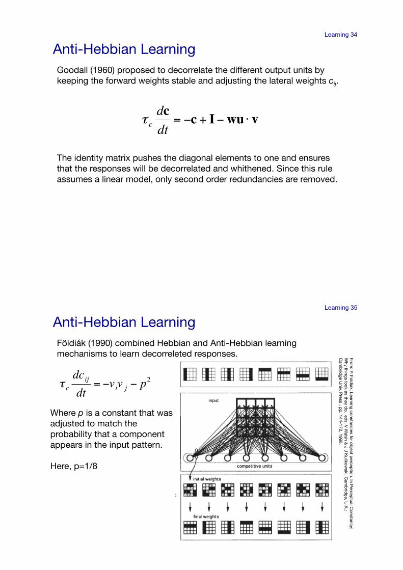
Goodall (1960) proposed to decorrelate the different output units by keeping the forward weights stable and adjusting the lateral weights cij.!
!
" cdcdt
= #c + I#wu $ v
The identity matrix pushes the diagonal elements to one and ensures that the responses will be decorrelated and whithened. Since this rule assumes a linear model, only second order redundancies are removed.!
Anti-Hebbian Learning!
Learning 35
Földiák (1990) combined Hebbian and Anti-Hebbian learning mechanisms to learn decorreleted responses.!
!
" cdcijdt
= #viv j # p2
Where p is a constant that was adjusted to match the probability that a component appears in the input pattern.!
Here, p=1/8!
From: P. Fold
iak, Learning constancies for object p
erception. In P
erceptual C
onstancy: W
hy things look as they do, ed
s. V W
alsh & J J K
ulikowski, C
amb
ridge, U
.K.:
Cam
brid
ge Univ. P
ress , pp
. 144-172, 1998.!
Anti-Hebbian Learning!
Learning 36
Anti-Hebbian learning is a very flexible mechanism that can also be used in non-linear neurons. In this case, higher order dependencies are also considered which will lead to largely independent responses.!
Anti-Hebbian Learning!
Learning 37
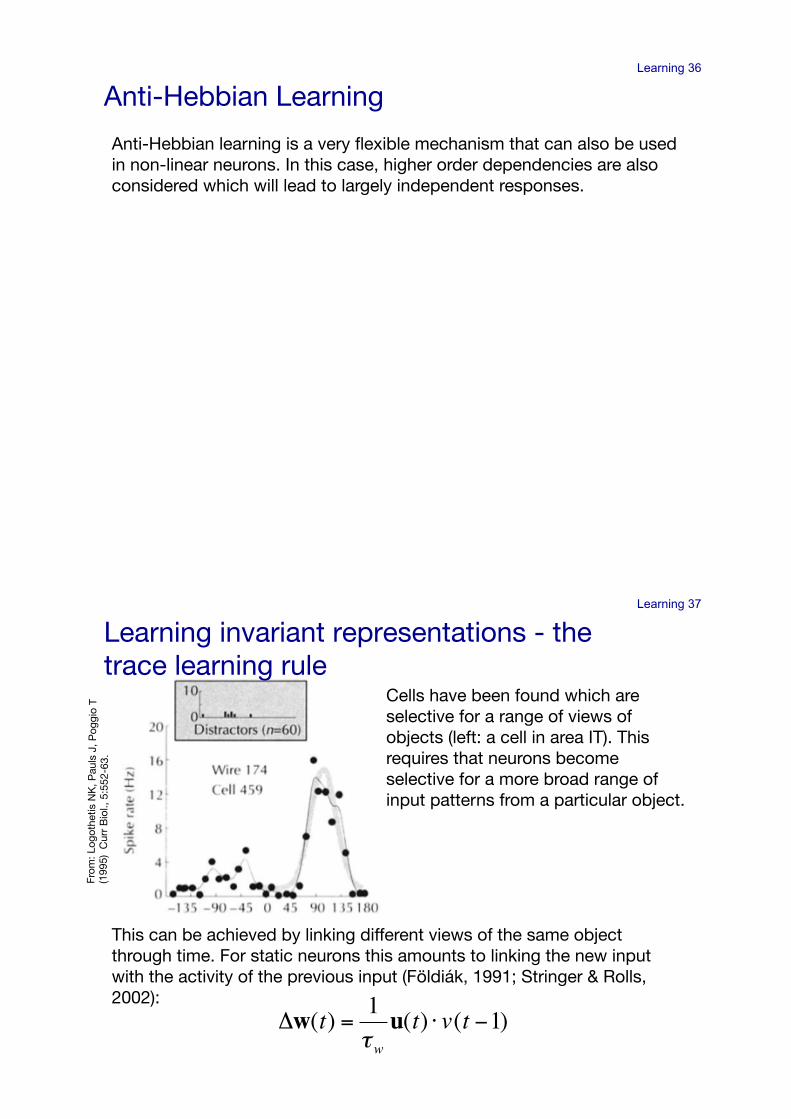
This can be achieved by linking different views of the same object through time. For static neurons this amounts to linking the new input with the activity of the previous input (Földiák, 1991; Stringer & Rolls, 2002):!
!
"w(t) =1#wu(t) $ v(t %1)
Cells have been found which are selective for a range of views of objects (left: a cell in area IT). This requires that neurons become selective for a more broad range of input patterns from a particular object.!
From
: Log
othe
tis N
K, P
auls
J, P
oggi
o T
(199
5) C
urr
Bio
l., 5
:552
-63.!
Learning invariant representations - the trace learning rule!
Learning 38
pre j
post i BPAP
Spike-based Hebbian Learning!
Learning 39
Spike-based Hebbian Learning!
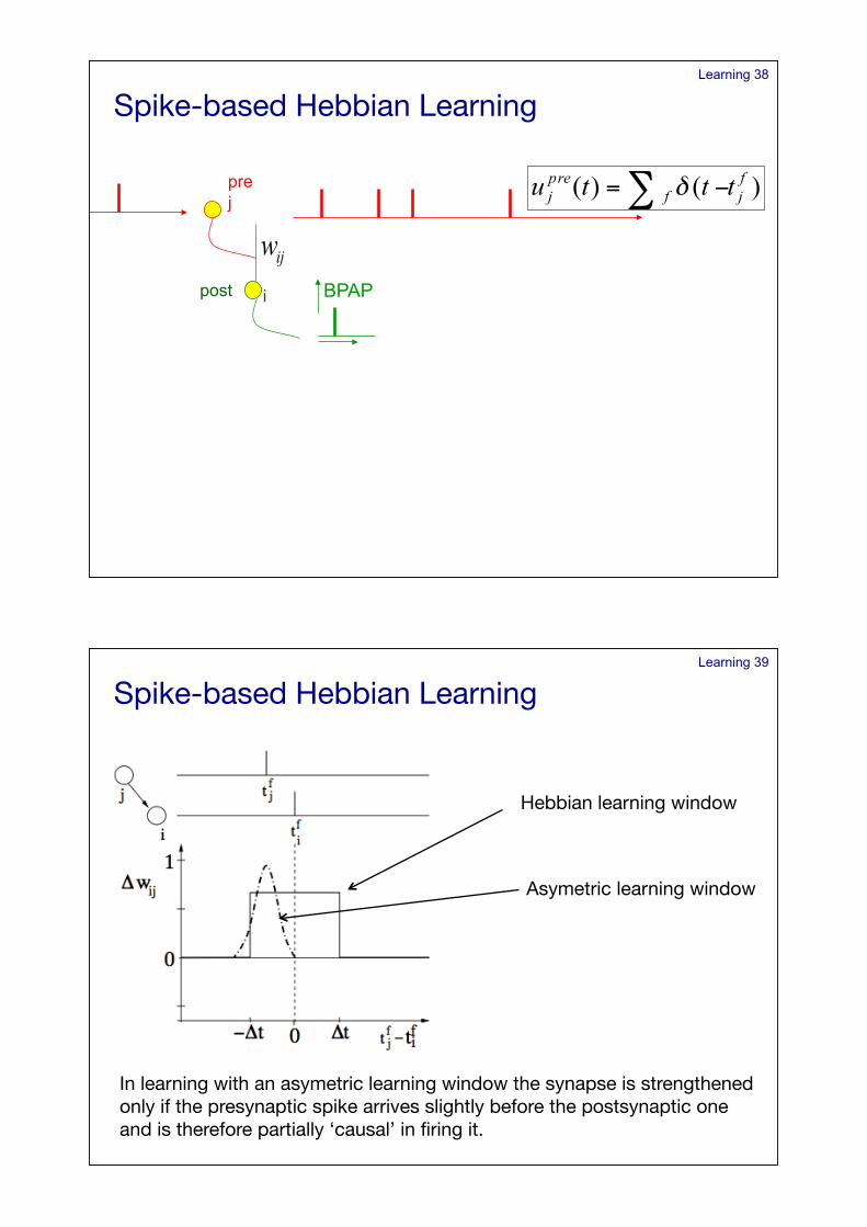
Hebbian learning window!
Asymetric learning window!
In learning with an asymetric learning window the synapse is strengthened only if the presynaptic spike arrives slightly before the postsynaptic one and is therefore partially ‘causal’ in firing it.!
Learning 40
Spike-Timing Dependent Plasticity (STDP)!
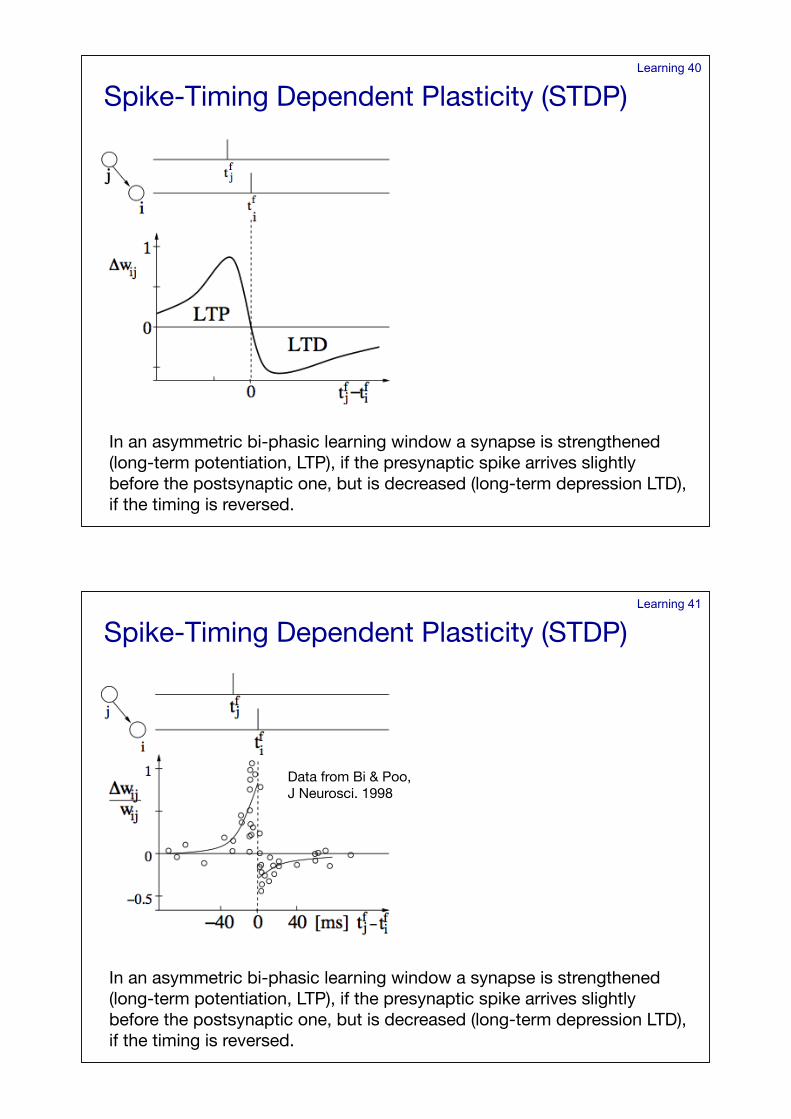
In an asymmetric bi-phasic learning window a synapse is strengthened (long-term potentiation, LTP), if the presynaptic spike arrives slightly before the postsynaptic one, but is decreased (long-term depression LTD), if the timing is reversed.!
Learning 41
Spike-Timing Dependent Plasticity (STDP)!
In an asymmetric bi-phasic learning window a synapse is strengthened (long-term potentiation, LTP), if the presynaptic spike arrives slightly before the postsynaptic one, but is decreased (long-term depression LTD), if the timing is reversed.!
Data from Bi & Poo, !J Neurosci. 1998!
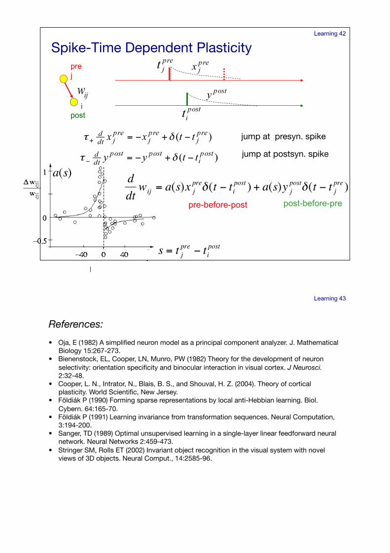
Learning 42
!
s = t jpre " ti
post
!
a(s)
pre j
post i
jump at presyn. spike!
jump at postsyn. spike!
pre-before-post post-before-pre
!
ddtwij = a(s)x j
pre"(t # tipost ) + a(s)y j
post"(t # t jpre )
Spike-Time Dependent Plasticity!
Learning 43
References:!
• Oja, E (1982) A simplified neuron model as a principal component analyzer. J. Mathematical Biology 15:267-273.!
• Bienenstock, EL, Cooper, LN, Munro, PW (1982) Theory for the development of neuron selectivity: orientation specificity and binocular interaction in visual cortex. J Neurosci. 2:32-48.!
• Cooper, L. N., Intrator, N., Blais, B. S., and Shouval, H. Z. (2004). Theory of cortical plasticity. World Scientific, New Jersey.!
• Földiák P (1990) Forming sparse representations by local anti-Hebbian learning. Biol. Cybern. 64:165-70.!
• Földiák P (1991) Learning invariance from transformation sequences. Neural Computation, 3:194-200.!
• Sanger, TD (1989) Optimal unsupervised learning in a single-layer linear feedforward neural network. Neural Networks 2:459-473.!
• Stringer SM, Rolls ET (2002) Invariant object recognition in the visual system with novel views of 3D objects. Neural Comput., 14:2585-96.!