Embed Size (px)
Citation preview

1
Learning Bayesian Networks(part 2)
Mark Craven and David PageComputer Sciences 760
Spring 2018
www.biostat.wisc.edu/~craven/cs760/
Some of the slides in these lectures have been adapted/borrowed from materials developed by Tom Dietterich, Pedro Domingos, Tom Mitchell, David Page, and Jude Shavlik
Goals for the lectureyou should understand the following concepts
• the Chow-Liu algorithm for structure search• structure learning as search• Kullback-Leibler divergence• the Sparse Candidate algorithm

2
Learning structure + parameters
• number of structures is superexponential in the number of variables
• finding optimal structure is NP-complete problem• two common options:
– search very restricted space of possible structures(e.g. networks with tree DAGs)
– use heuristic search (e.g. sparse candidate)
The Chow-Liu algorithm
• learns a BN with a tree structure that maximizes the likelihood of the training data
• algorithm1. compute weight I(Xi, Xj) of each possible edge (Xi, Xj)2. find maximum weight spanning tree (MST)3. assign edge directions in MST
3
The Chow-Liu algorithm
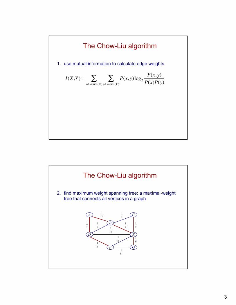
1. use mutual information to calculate edge weights
I(X,Y ) = P(x, y)log2y∈ values(Y )∑ P(x, y)
P(x)P(y)x∈ values(X )∑
The Chow-Liu algorithm
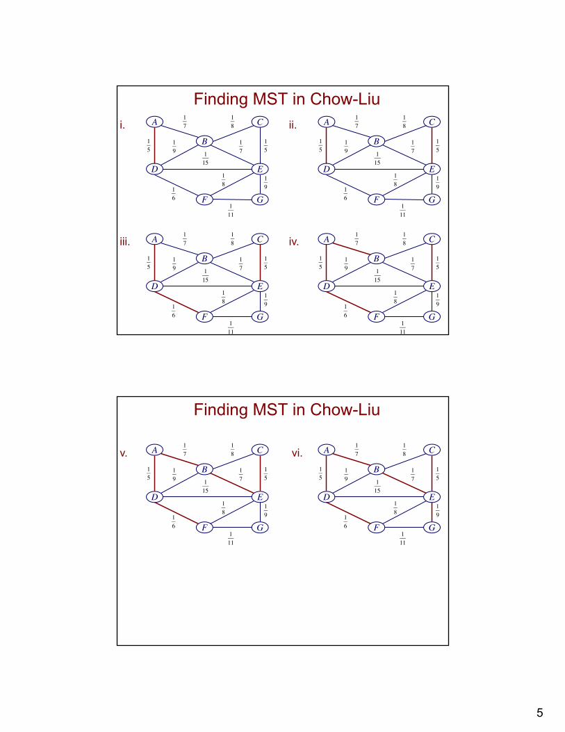
2. find maximum weight spanning tree: a maximal-weight tree that connects all vertices in a graph
A
B
C
D E
F G
15
15
17
18
19
171
15
16
18
19
111
4
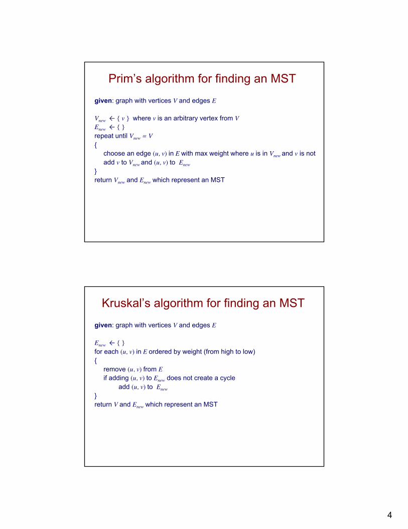
Prim’s algorithm for finding an MSTgiven: graph with vertices V and edges E
Vnew ← { v } where v is an arbitrary vertex from VEnew ← { } repeat until Vnew = V{
choose an edge (u, v) in E with max weight where u is in Vnew and v is notadd v to Vnew and (u, v) to Enew
}return Vnew and Enew which represent an MST
Kruskal’s algorithm for finding an MSTgiven: graph with vertices V and edges E
Enew ← { } for each (u, v) in E ordered by weight (from high to low){
remove (u, v) from Eif adding (u, v) to Enew does not create a cycle
add (u, v) to Enew}return V and Enew which represent an MST
5
Finding MST in Chow-LiuA
B
C
D E
F G
15
15
17
18
19
171
15
16
18
19
111
i. A
B
C
D E
F G
15
15
17
18
19
171
15
16
18
19
111
ii.
A
B
C
D E
F G
15
15
17
18
19
171
15
16
18
19
111
iii. A
B
C
D E
F G
15
15
17
18
19
171
15
16
18
19
111
iv.
Finding MST in Chow-Liu
A
B
C
D E
F G
15
15
17
18
19
171
15
16
18
19
111
v. A
B
C
D E
F G
15
15
17
18
19
171
15
16
18
19
111
vi.
6
Returning directed graph in Chow-Liu
A
B
C
D E
F G
A
B
C
D E
F G
15
15
17
18
19
171
15
16
18
19
111
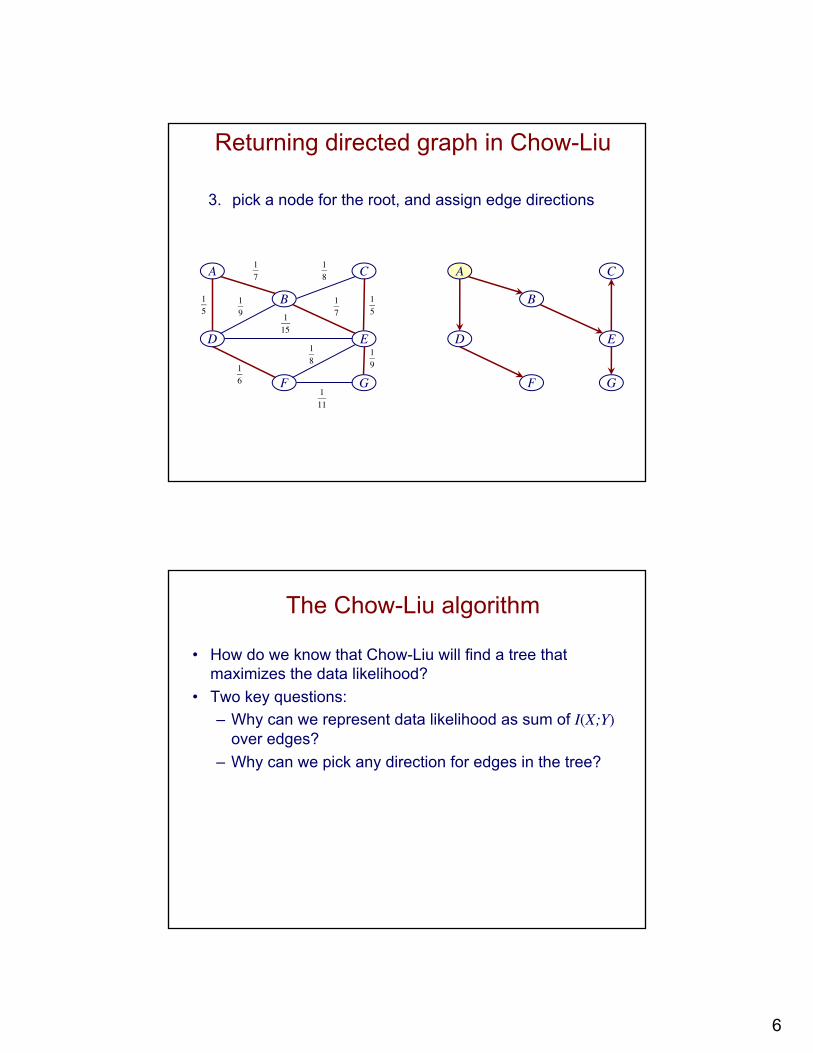
3. pick a node for the root, and assign edge directions
The Chow-Liu algorithm
• How do we know that Chow-Liu will find a tree that maximizes the data likelihood?
• Two key questions:– Why can we represent data likelihood as sum of I(X;Y)
over edges?– Why can we pick any direction for edges in the tree?

7
Why Chow-Liu maximizes likelihood (for a tree)
log2 P(D |G,θG ) = log2 P(xi(d ) | Parents(Xi ))
i∑
d∈D∑
= D I(Xi ,Parents(Xi ))− H (Xi )( )i∑
data likelihood given directed edges
argmaxG log2 P(D |G,θG ) = argmaxG I(Xi ,Parents(Xi ))i∑
we’re interested in finding the graph G that maximizes this
argmaxG log2 P(D |G,θG ) = argmaxG I(Xi ,Xj )(Xi ,X j )∈edges∑
if we assume a tree, each node has at most one parent
I(Xi ,Xj ) = I(Xj ,Xi )edge directions don’t matter for likelihood, because MI is symmetric
Heuristic search for structure learning
• each state in the search space represents a DAG Bayesnet structure
• to instantiate a search approach, we need to specify– scoring function– state transition operators– search algorithm

8
Scoring function decomposability
• when the appropriate priors are used, and all instances in D are complete, the scoring function can be decomposed as follows
score(G, D) = score(Xi
i∑ ,Parents(Xi ) :D)
• thus we can– score a network by summing terms over the nodes in
the network
– efficiently score changes in a local search procedure
Scoring functions for structure learning• Can we find a good structure just by trying to maximize the
likelihood of the data?
argmaxG , θG logP(D |G,θG )
• If we have a strong restriction on the the structures allowed (e.g. a tree), then maybe.
• Otherwise, no! Adding an edge will never decrease likelihood. Overfitting likely.

9
Scoring functions for structure learning• there are many different scoring functions for BN structure
search• one general approach
argmaxG , θG logP(D |G,θG )− f (m)θG
complexity penalty
Akaike Information Criterion (AIC): f (m) = 1
Bayesian Information Criterion (BIC): f (m) =12log(m)
Structure search operators
A
B C
D
A
B C
D
add an edge
A
B C
D
reverse an edge
given the current networkat some stage of the search, we can…
A
B C
D
delete an edge

10
Bayesian network search: hill-climbing
given: data set D, initial network B0
i = 0Bbest ←B0
while stopping criteria not met{
for each possible operator application a{
Bnew ← apply(a, Bi)if score(Bnew) > score(Bbest)
Bbest ← Bnew}++iBi ← Bbest
}return Bi
Bayesian network search: the Sparse Candidate algorithm
[Friedman et al., UAI 1999]
given: data set D, initial network B0, parameter k
i = 0repeat{
++i
// restrict stepselect for each variable Xj a set Cj
i of candidate parents (|Cji| ≤ k)
// maximize stepfind network Bi maximizing score among networks where ∀Xj, Parents(Xj) ⊆Cj
i
} until convergencereturn Bi
11
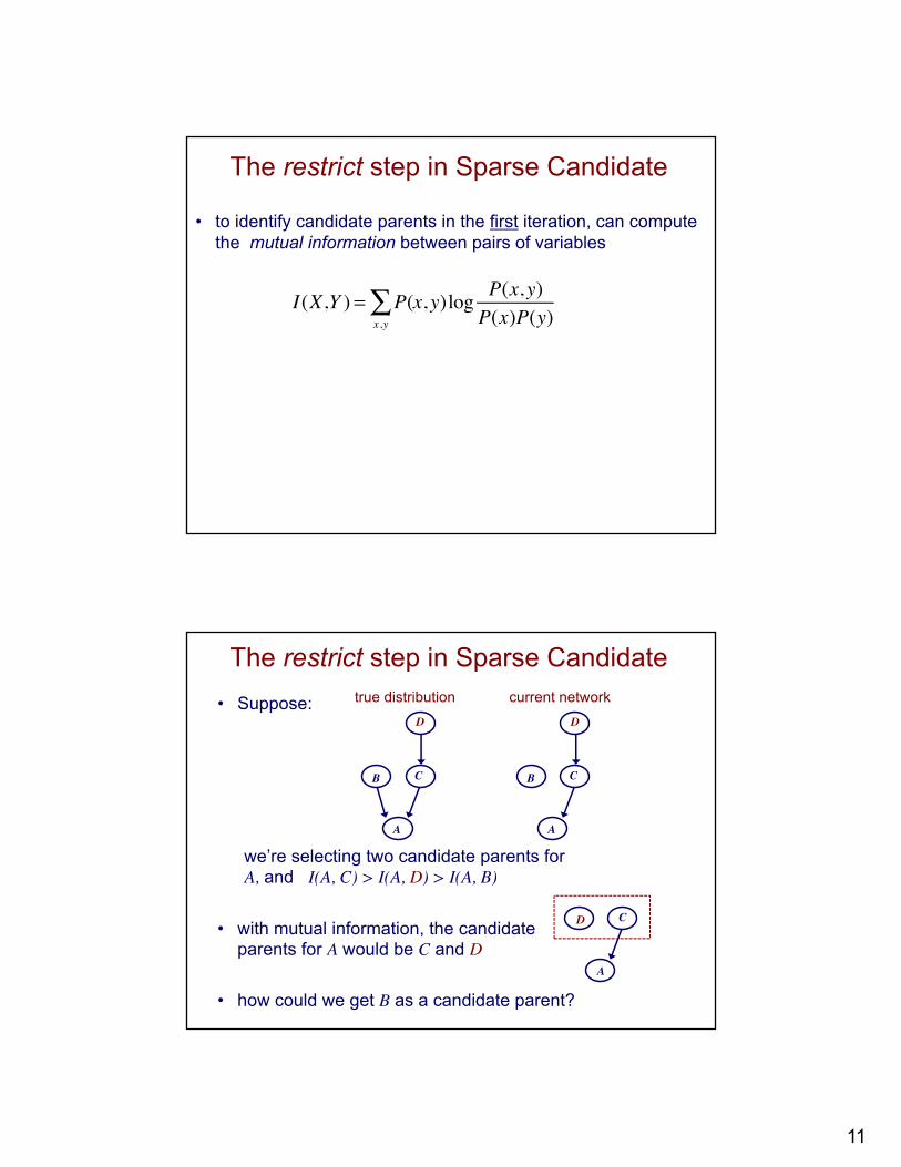
• to identify candidate parents in the first iteration, can compute the mutual information between pairs of variables
The restrict step in Sparse Candidate
I(X,Y ) = P(x,y∑ x, y)log P(x, y)
P(x)P(y)
• Suppose:
we’re selecting two candidate parents for A, and I(A, C) > I(A, D) > I(A, B)
• with mutual information, the candidate parents for A would be C and D
• how could we get B as a candidate parent?
A
B C
D
A
D C
The restrict step in Sparse Candidate
A
B C
D
true distribution current network
12
)()(
log)())(||)((xQxP
xPXQXPDx
KL ∑=
• mutual information can be thought of as the KL divergence between the distributions
• Kullback-Leibler (KL) divergence provides a distance measure between two distributions, P and Q
P(X,Y )
P(X)P(Y ) (assumes X and Y are independent)
The restrict step in Sparse Candidate
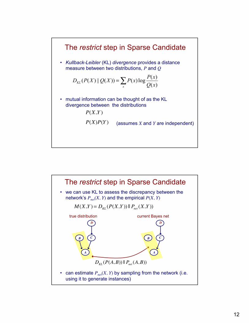
• we can use KL to assess the discrepancy between the network’s Pnet(X, Y) and the empirical P(X, Y)
M (X,Y ) = DKL (P(X,Y )) || Pnet (X,Y ))
A
B C
D
true distribution current Bayes net
DKL (P(A,B)) || Pnet (A,B))
The restrict step in Sparse Candidate
• can estimate Pnet(X, Y) by sampling from the network (i.e. using it to generate instances)
A
B C
D
13
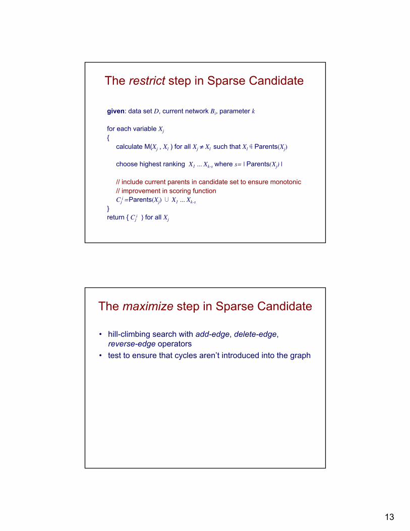
The restrict step in Sparse Candidate
given: data set D, current network Bi, parameter k
for each variable Xj{
calculate M(Xj , Xl ) for all Xj ≠ Xl such that Xl ∉ Parents(Xj)
choose highest ranking X1 ... Xk-s where s= | Parents(Xj) |
// include current parents in candidate set to ensure monotonic// improvement in scoring functionCj
i =Parents(Xj) ∪ X1 ... Xk-s} return { Cj
i } for all Xj
The maximize step in Sparse Candidate
• hill-climbing search with add-edge, delete-edge,reverse-edge operators
• test to ensure that cycles aren’t introduced into the graph
14
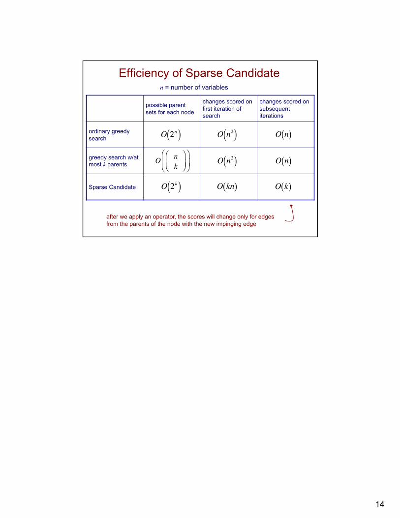
Efficiency of Sparse Candidate
possible parent sets for each node
changes scored on first iteration of search
changes scored on subsequent iterations
ordinary greedy search
greedy search w/at most k parents
Sparse Candidate
�
O 2k( )�
O 2n( )
�
O n2( )
�
O n2( )
�
O kn( )�
O n( )
�
O n( )
�
O k( )
O nk
⎛⎝⎜
⎞⎠⎟
⎛
⎝⎜⎞
⎠⎟
n = number of variables
after we apply an operator, the scores will change only for edges from the parents of the node with the new impinging edge