Embed Size (px)
Citation preview
LM-FL-1
1
Learning Module 3
Fluid Analysis
Title Page Guide
What is a Learning Module?
A Learning Module (LM) is a structured, concise, and self-sufficient learning resource. An
LM provides the learner with the required content in a precise and concise manner, enabling
the learner to learn more efficiently and effectively. It has a number of characteristics that
distinguish it from a traditional textbook or textbook chapter:
An LM is learning objective driven, and its scope is clearly defined and bounded. The
module is compact and precise in presentation, and its core material contains only
contents essential for achieving the learning objectives. Since an LM is inherently
concise, it can be learned relatively quickly and efficiently.
An LM is independent and free-standing. Module-based learning is therefore non-
sequential and flexible, and can be personalized with ease.
Presenting the material in a contained and precise fashion will allow the user to learn
effectively, reducing the time and effort spent and ultimately improving the learning
experience. This is the first module on thermal analysis and provides the user with the
necessary tools to complete a thermal FEM study with different boundary conditions. It goes
through all of the steps necessary to successfully complete an analysis, including geometry
creation, material selection, boundary condition specification, meshing, solution, and
validation. These steps are first covered conceptually and then worked through directly as
they are applied to an example problem.
Estimated Learning Time for This Module
Estimated learning time for this LM is equivalent to three 50-minute lectures, or one week of
study time for a 3 credit hour course.
How to Use This Module
The learning module is organized in sections. Each section contains a short explanation and a
link to where that section can be found. The explanation will give you an idea of what
content is in each section. The link will allow you to complete the parts of the module you
are interested in, while being able to skip any parts that you might already be familiar with.
The modularity of the LM allows for an efficient use of your time.
LM-FL-1
2
Table of Contents
1. Learning Objectives ................................................................................................................ 3 2. Prerequisites ............................................................................................................................ 3 3. Pre-test .................................................................................................................................... 3 4. Tutorial Problem Statements................................................................................................... 4 5. Conceptual Analysis ............................................................................................................... 7 6. Abstract Modeling .................................................................................................................. 8 7. Software-Specific FEM Tutorials ........................................................................................... 8 8. Post-test ................................................................................................................................... 8 9. Practice Problems.................................................................................................................... 8 10. Assessment ............................................................................................................................ 9 Attachment A. Pre-Test ............................................................................................................ 10 Attachment B. Conceptual Analysis ......................................................................................... 12 Attachment C1. SolidWorks-Specific FEM Tutorial 1............................................................. 15 Attachment C2. SolidWorks-Specific FEM Tutorial 2............. Error! Bookmark not defined. Attachment C3. SolidWorks-Specific FEM Tutorial 3............. Error! Bookmark not defined. Attachment D. CoMetSolution-Specific FEM Tutorials .......................................................... 48 Attachment E. Post-Test ........................................................................................................... 71 Attachment F. Practice Problems .............................................................................................. 73 Attachment G. Solutions to Practice Problems ......................................................................... 79 Attachment H. Assessment ....................................................................................................... 85
LM-FL-1
3
1. Learning Objectives
The objective of this module is to introduce the user to the process of fluid flow analysis using
FEM. Upon completion of the module, the user should have a good understanding of the
necessary logical steps of an FEM analysis, and be able to perform the following tasks:
Creating the solid geometry
Assigning material properties
Applying boundary conditions
Meshing
Running the analysis
Verifying model correctness
Processing needed results
2. Prerequisites
In order to complete the learning module successfully, the following prerequisites are required:
By subject area:
o Fluid mechanics
o Flow analysis
By topic:
knowledge of
o fluid boundary layer
o laminar flow
o turbulent flow
o Reynolds number
o volumetric flow rate
o pressure drop
o drag force
o fluid properties
3. Pre-test
The pre-test should be taken before taking other sections of the module. The purpose of the pre-
test is to assess the user's prior knowledge in subject areas relevant to fluid flow analysis.
Questions are focused towards fundamental concepts including types of flow, fluid definitions,
and various boundary conditions.
The pre-test for this module given in Attachment I.
Link to Pre-test
LM-FL-1
4
4. Tutorial Problem Statements
A good tutorial problem should focus on the logical steps in FEM modeling and demonstrate as
many aspects of the FEM software as possible. It should also be simple in mechanics with an
analytical solution available for validation. Three tutorial problems are covered in this learning
module.
Tutorial Problem 1
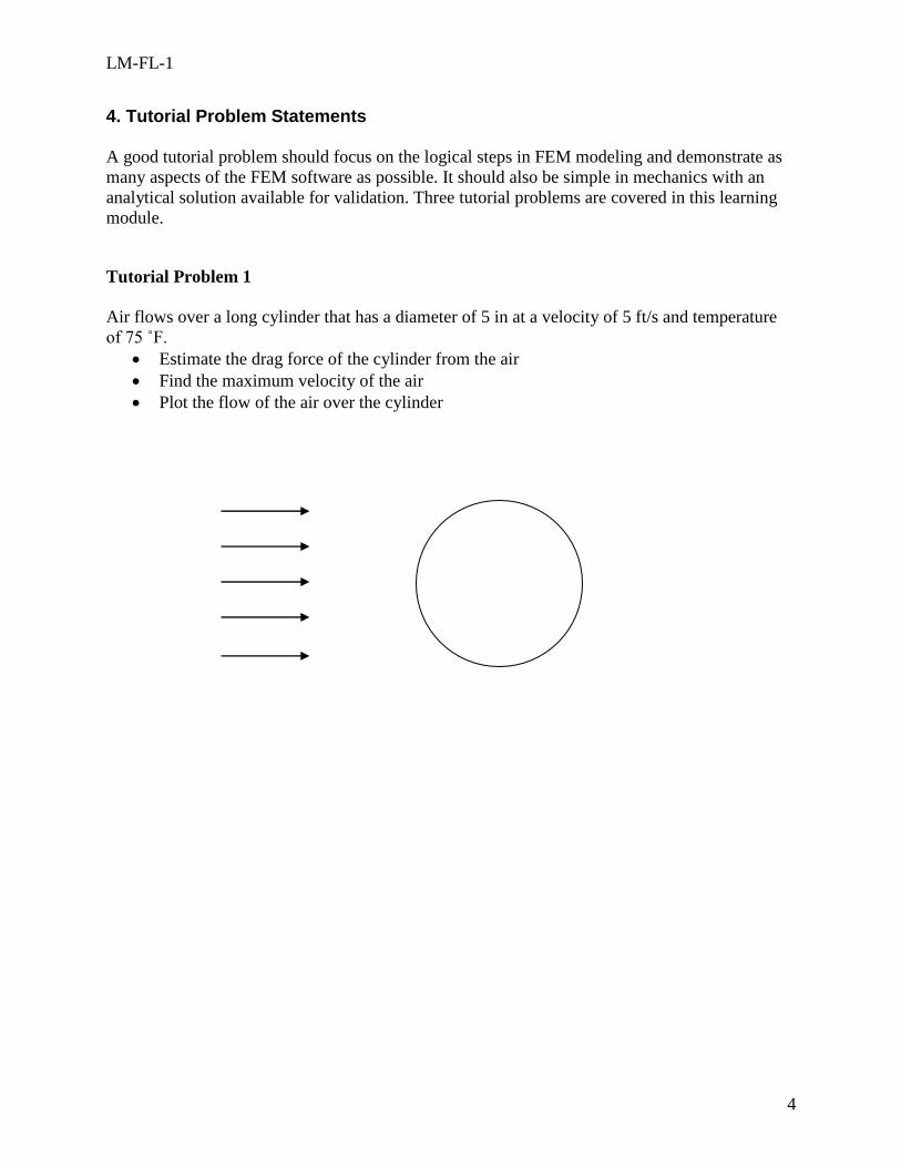
Air flows over a long cylinder that has a diameter of 5 in at a velocity of 5 ft/s and temperature
of 75 ˚F.
Estimate the drag force of the cylinder from the air
Find the maximum velocity of the air
Plot the flow of the air over the cylinder

LM-FL-1
5
Tutorial Problem 2
Air flows through a rectangular duct at 200 cfm into a 10x10x10 room and exits through a
circular duct and releases into the atmosphere as in the figure below. The rectangular duct is
18x6 inches and the circular duct has a diameter of 12 inches.
Graph and animate the flow trajectory of the air
Find the velocity through the rectangular and circular duct sections
LM-FL-1
6
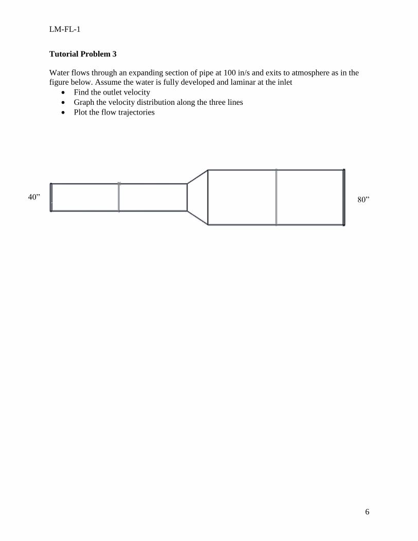
Tutorial Problem 3
Water flows through an expanding section of pipe at 100 in/s and exits to atmosphere as in the
figure below. Assume the water is fully developed and laminar at the inlet
Find the outlet velocity
Graph the velocity distribution along the three lines
Plot the flow trajectories
40” 80”
LM-FL-1
7
5. Conceptual Analysis
Conceptual analysis is the abstraction of the logical steps in performing a task or solving a
problem. Conceptual analysis for FEM simulation is problem type dependent but software-
independent, and is fundamental in understanding and solving the problem.
Conceptual analysis for static structural analysis reveals the following general logical steps:
1. Pre-processing
o Geometry creation
o Material property assignment
o Boundary condition specification
o Mesh generation
2. Solution
3. Post-processing
4. Validation
Attachment II discusses the conceptual analysis for the tutorial problems in this module.
Link to Conceptual Analysis
LM-FL-1
8
6. Abstract Modeling
Abstract modeling is a process pioneered by CometSolutions Inc. Abstract modeling enables all
attributes of an FEM model (such as material properties, constraints, loads, mesh, etc.) to be
defined independently in an abstract fashion, thus reducing model complexity without affecting
model accuracy with respect to the simulation objective. It detaches attributes from one another,
and emphasizes conceptual understanding rather than focusing on software specifics. Evidently,
abstract modeling is independent of the specific software being used. This is a fundamental
departure from the way most FEM packages operate.
Conceptual analysis focuses on the abstraction of steps necessary for an FEM simulation, while
abstract modeling focuses on the abstraction and modularization of attributes that constitute an
FEM model. They are powerful enabling instruments in FEM teaching and learning.
Link to Abstract Modeling
7. Software-Specific FEM Tutorials
In software-specific FEM tutorial section, the tutorial problem is solved step by step in a
particular software package. This section fills in the details of the conceptual analysis as outlined
in previous section. It provides step by step details that correspond to the pre-processing,
solution, post-processing and validation phases using a particular software package.
Two commercial FEM packages are covered in this module: SolidWorks and CometSolution.
Below are the two links:
Link to SolidWorks FEM Tutorial 1
Link to SolidWorks FEM Tutorial 2
Link to SolidWorks FEM Tutorial 3
Link to CometSolution FEM Tutorials
8. Post-test
The post-test will be taken upon completion of the module. The first part of the post-test is from
the pre-test to test knowledge gained by the user, and the second part is focused on the FEM
simulation process covered by the tutorial.
Link to Post-Test
9. Practice Problems
The user should be able to solve practice problems after completing this module. The practice
problems provide a good reinforcement of the knowledge and skills learned in the module, and
LM-FL-1
9
can be assigned as homework problems in teaching or self study problems to enhance learning.
These problems are similar to the tutorial problems worked in the module, but they involve
different geometries and thermal boundary conditions.
Link to Practice Problems
Link to Solutions for Practice Problems
10. Assessment
The assessment is provided as a way to receive feedback about the module. The user evaluates
several categories of the learning experience, including interactive learning, the module format,
its effectiveness and efficiency, the appropriateness of the sections, and the overall learning
experience. There is also the opportunity to give suggestions or comments about the module.
Link to Assessment

LM-FL-1
10
Attachment A. Pre-Test
1. The velocity of a fluid through an opening is dependent on
o Volumetric flow rate
o Cross-sectional area of the opening
o Fluid distance from the surface
o All the above
2. Fully developed flow through a pipe is most likely to be found
o Towards the end of the pipe
o At the beginning of the pipe
o After a turn in the pipe
o After a pump or fan
3. Which of the following is true about the velocity in the boundary layer?
o The velocity is zero at the surface
o The velocity increases when the distance from the surface increases
o The boundary layer thickness is the distance from the surface to the point where the fluid
reaches maximum velocity
o All of the above
4. Which of the following is not a characteristic of turbulent flow?
o Irregular movement of fluid particles
o Eddies and vortices
o High Reynolds number
o Low Reynolds number
5. What scientific principle relates a fluid’s speed, pressure and potential energy?
o Archimedes’s principle
o Bernoulli’s principle
o Le Chatelier’s principle
o Mach’s principle
6. Which branch of physics deals with the forces acting on bodies passing through air and other
gaseous fluids?
o Thermodynamics
o Dynamics

LM-FL-1
11
o Aerodynamics
o Biomechanics
7. Which of the following values are not needed to calculate the drag force of a fluid flowing
towards a flat plate?
o Fluid type
o Fluid velocity
o Area of the plate
o Density of the plate
8. What quantity is used to describe the resistance to fluid flow?
o Lift coefficient
o Mach number
o Drag coefficient
o Reynolds number
9. What dimensionless parameter is used to determine if the flow is laminar, transitional, or
turbulent?
o Reynolds number
o Prandtl number
o Biot number
o Mach number
10. Which of the following is not a boundary condition in flow analysis?
o Inlet volumetric flow rate
o Environmental pressure
o Outlet force
o Outlet velocity
Click to continue
LM-FL-1
12
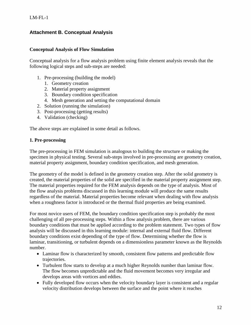
Attachment B. Conceptual Analysis
Conceptual Analysis of Flow Simulation
Conceptual analysis for a flow analysis problem using finite element analysis reveals that the
following logical steps and sub-steps are needed:
1. Pre-processing (building the model)
1. Geometry creation
2. Material property assignment
3. Boundary condition specification
4. Mesh generation and setting the computational domain
2. Solution (running the simulation)
3. Post-processing (getting results)
4. Validation (checking)
The above steps are explained in some detail as follows.
1. Pre-processing
The pre-processing in FEM simulation is analogous to building the structure or making the
specimen in physical testing. Several sub-steps involved in pre-processing are geometry creation,
material property assignment, boundary condition specification, and mesh generation.
The geometry of the model is defined in the geometry creation step. After the solid geometry is
created, the material properties of the solid are specified in the material property assignment step.
The material properties required for the FEM analysis depends on the type of analysis. Most of
the flow analysis problems discussed in this learning module will produce the same results
regardless of the material. Material properties become relevant when dealing with flow analysis
when a roughness factor is introduced or the thermal fluid properties are being examined.
For most novice users of FEM, the boundary condition specification step is probably the most
challenging of all pre-processing steps. Within a flow analysis problem, there are various
boundary conditions that must be applied according to the problem statement. Two types of flow
analysis will be discussed in this learning module: internal and external fluid flow. Different
boundary conditions exist depending of the type of flow. Determining whether the flow is
laminar, transitioning, or turbulent depends on a dimensionless parameter known as the Reynolds
number.
Laminar flow is characterized by smooth, consistent flow patterns and predictable flow
trajectories.
Turbulent flow starts to develop at a much higher Reynolds number than laminar flow.
The flow becomes unpredictable and the fluid movement becomes very irregular and
develops areas with vortices and eddies.
Fully developed flow occurs when the velocity boundary layer is consistent and a regular
velocity distribution develops between the surface and the point where it reaches

LM-FL-1
13
maximum velocity. At the surface, the velocity is zero due to shear forces but as the fluid
moves farther away from the surface the velocity increases to its maximum value.
Other boundary conditions and properties also exist in a flow analysis including:
Volumetric flow rate – the rate (usually expressed in ft3/min or m
3/s) at which the fluid
flows through an enclosed space. The volumetric flow rate is constant through an
enclosed volume and is found by multiplying the velocity by the cross sectional area of
the space.
Drag force – the force of the object moving through a fluid. The drag force points in the
direction of the fluid velocity and can be applied situations such as a car moving though
air or a sphere moving through water. The coefficient of drag can be calculated from this
parameter and relates the drag force with the velocity of the air and other fluid factors to
reduce the number into a comparable dimensionless quantity.
Mesh generation is the process of discretizing the body into finite elements and assembling the
discrete elements into an integral structure that approximates the original body. Most FEM
packages have their own default meshing parameters to mesh the model and run the analysis
while providing ways for the user to refine the mesh.
The computational domain is the area that the simulation software runs the calculations. For
external analysis, the computational domain can be increased or reduced depending on the
amount of data required. Internal flow analysis requires the computational domain to be greater
than the enclosed volume.
2. Solution
The solution is the process of solving the governing equations resulting from the discretized
FEM model. Although the mathematics for the solution process can be quite involved, this step
is transparent to the user and is usually as simple as clicking a solution button or issuing the
solution command.
3. Post-processing
The purpose of an FEM analysis is to obtain wanted results, and this is what the post-processing
step is for. Typically, various components or goals such as flow rate, velocity, or pressure at any
given location in the model are available. The way a quantity is outputted depends on the FEM
software.
4. Validation
Although validation is not a formal part of the FEM analysis, it is important to be included.
Blindly trusting a simulation without checking its correctness can be dangerous. The validation
usually involves comparing FEM results at one or more selected positions with exact or
approximate solutions using classical approaches learned in fluid mechanics courses. Going
through validation strengthens conceptual understanding and enhances learning.

LM-FL-1
14
Conceptual Analysis of a Given Problem
This section will give an example of conceptual analysis that will be applied to the first tutorial
problem. The goal of the FEM simulation is to correctly set up the boundary conditions and then
find the temperature at various nodes. The problem shows a table frame with a given material
and four temperature boundaries applied to the legs. Conceptual analysis of the current problem
is described as follows.
1. Pre-processing (building the model)
The geometry of the structure is first created using the design feature of the FEM package. Next,
a material is assigned to the solid model and the boundary conditions are specified. This problem
is an external analysis and has various initial parameters such as temperature, pressure and
velocity that need to be applied.
The next step is to mesh the solid to discretize it into finite elements. Generally, commercial
FEA software has automatic default meshing parameters such as average element size of the
mesh, quality of the mesh, etc. Here the default parameters provided by the software are used.
2. Solution (running the simulation)
The next step is to run the simulation and obtain a solution. Usually the software provides
several solver options. The default solver usually works well. For some problems, a particular
solver may be faster or give more accurate results.
3. Post-processing (getting results)
After the analysis is complete, the post-processing steps are performed. Results such as velocity,
pressure, force, etc. can be calculated and plotted using the simulation software. Some software
packages will also output wanted information to a spreadsheet and graph the data.
4. Validation (checking)
Validation is the final step in the analysis process. In this step, drag force and maximum velocity
are calculated and compared with the software generated results to check the validity of the
analysis.
This completes the Conceptual Analysis section. Click the link below to continue with the
learning module.
Click to continue

LM-FL-1
15
Attachment C1. SolidWorks-Specific FEM Tutorial 1
Overview: In this section, three tutorial problems will be solved using the commercial FEM
software SolidWorks. Although the underlying principles and logical steps of an FEM simulation
identified in the Conceptual Analysis section are independent of any particular FEM software,
the realization of conceptual analysis steps will be software dependent. The SolidWorks-specific
steps are described in this section.
This is a step-by-step tutorial. However, it is designed such that those who are familiar with the
details in a particular step can skip it and go directly into the next step.
Tutorial Problem 1.
0. Launching SolidWorks
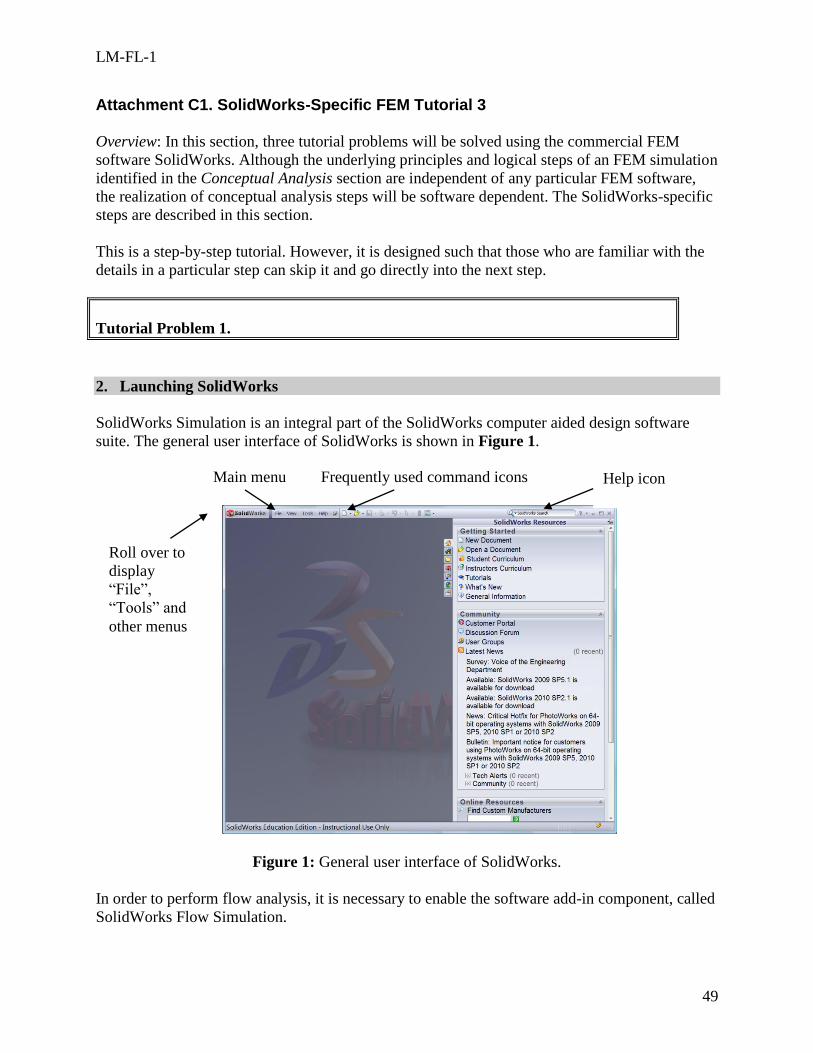
SolidWorks Simulation is an integral part of the SolidWorks computer aided design software
suite. The general user interface of SolidWorks is shown in Figure 1.
Figure 1: General user interface of SolidWorks.
In order to perform flow analysis, it is necessary to enable the software add-in component, called
SolidWorks Flow Simulation.
Main menu Frequently used command icons Help icon
Roll over to
display
“File”,
“Tools” and
other menus

LM-FL-1
16
Step 1: Enabling SolidWorks Flow Simulation
o Click Tools in the main menu and select Add-ins.... The Add-ins dialog window
appears, as shown in Figure 2.
o Check the boxes in both the Active Add-ins and Start Up columns corresponding to
SolidWorks Flow Simulation.
o Checking the Active Add-ins box enables SolidWorks to activate the Flow
Simulation package for the current session. Checking the Start Up box enables the
Flow Simulation package for all future sessions whenever SolidWorks starts up.
Figure 2: Location of the SolidWorks icon and the boxes to be checked for adding it to the
panel.
1. Pre-Processing
Purpose: The purpose of pre-processing is to create an FEM model for use in the next step of the
simulation, Solution. It consists of the following sub-steps:
Geometry creation
Material property assignment
Boundary condition specification
Mesh generation.
LM-FL-1
17
1.1 Geometry Creation
The purpose of Geometry Creation is to create a geometrical representation of the solid object or
structure to be analyzed. In SolidWorks, such a geometric model is called a part. In this tutorial,
the necessary part has already been created in SolidWorks. The following steps will open up the
part for use in the flow analysis.
Step 1: Opening the part for simulation. One of the following two options can be used.
o Option1: Double click the following icon to open the embedded part file,
Cylinder.SLDPRT, in SolidWorks
Click SolidWorks part file icon to open it ==>
o Option 2: Download the part file “Cylinder.SLDPRT” from the web site
http://www.femlearning.org/. Use the File menu in SolidWorks to open the
downloaded part.
The SolidWorks model tree will appear with the given part name at the top. Above the model
tree, there should be various tabs labeled Features, Sketch, etc. If the Flow Simulation tab is
not visible, go back to steps 1 and 2 to enable the SolidWorks
Flow Simulation package. SolidWorks Flow Simulation has two options to create a new project:
using the configuration wizard and creating a new project with default settings. In this situation,
the project configuration will be used to specify the initial conditions. The initial conditions
include temperature and velocity, which is 5 m/s in this situation. The direction of the velocity is
along the z-axis, however the z-axis points in the opposite direction so the velocity needs to be “-
5 m/s” to correctly apply the boundary condition.
Step 2: Using the flow simulation wizard to configure a new project
o Click the tab above the model tree
o Click the icon to create a new flow simulation study
o In the first step of the wizard, select Create new and type “Airflow past cylinder”
next to Configuration name and click Next >
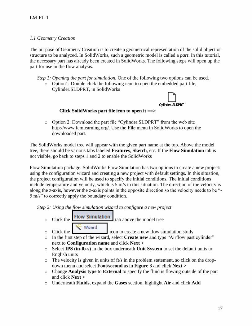
o Select IPS (in-lb-s) in the box underneath Unit System to set the default units to
English units
o The velocity is given in units of ft/s in the problem statement, so click on the drop-
down menu and select Foot/second as in Figure 3 and click Next >
o Change Analysis type to External to specify the fluid is flowing outside of the part
and click Next >
o Underneath Fluids, expand the Gases section, highlight Air and click Add
LM-FL-1
18
o Once Air (Gases) is added to the Project Fluids and the Default Fluid box is
checked, click Next >
o Leave the Default wall thermal condition as “Adiabatic wall” and Roughness at “0
microinch” and click Next >
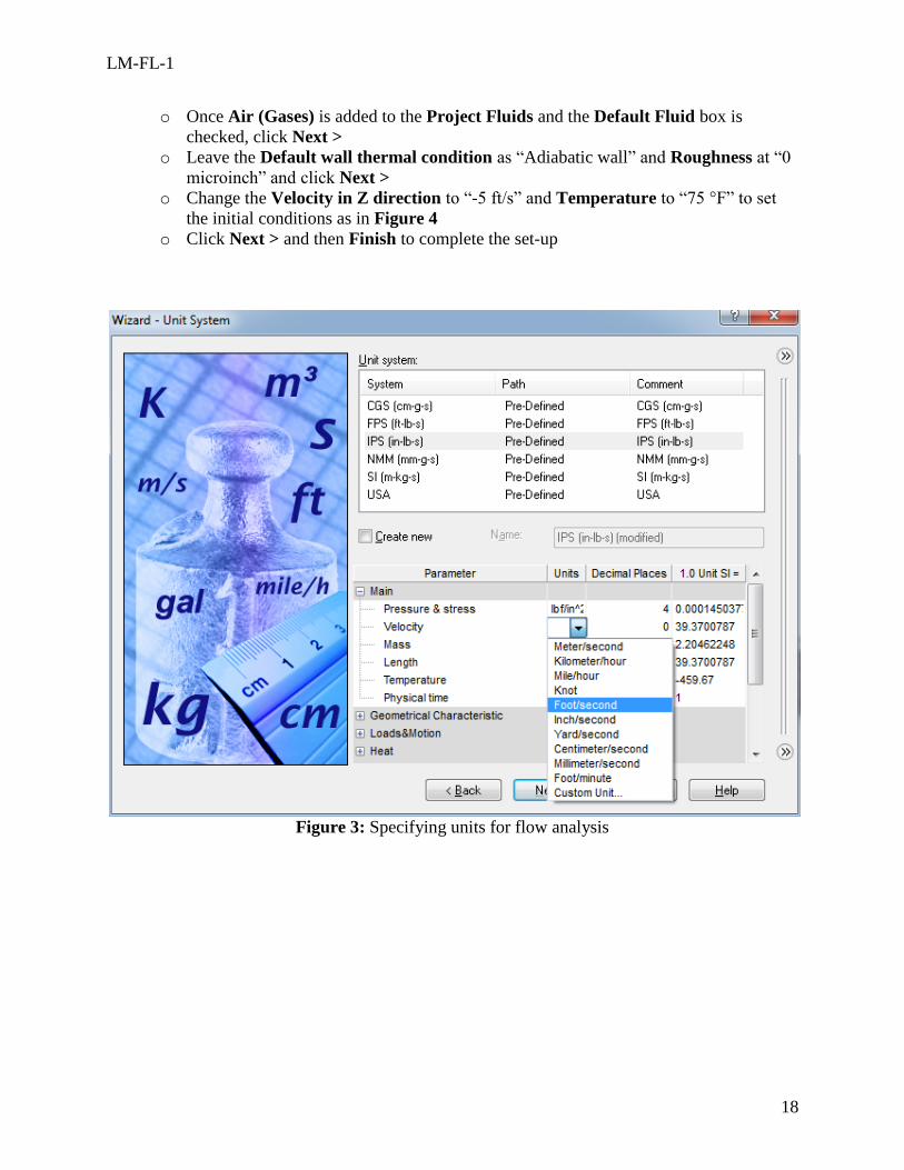
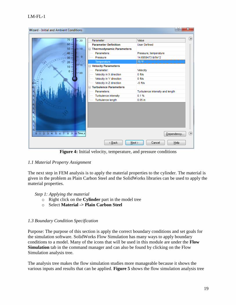
o Change the Velocity in Z direction to “-5 ft/s” and Temperature to “75 °F” to set
the initial conditions as in Figure 4
o Click Next > and then Finish to complete the set-up
Figure 3: Specifying units for flow analysis
LM-FL-1
19
Figure 4: Initial velocity, temperature, and pressure conditions
1.1 Material Property Assignment
The next step in FEM analysis is to apply the material properties to the cylinder. The material is
given in the problem as Plain Carbon Steel and the SolidWorks libraries can be used to apply the
material properties.
Step 1: Applying the material
o Right click on the Cylinder part in the model tree
o Select Material -> Plain Carbon Steel
1.3 Boundary Condition Specification
Purpose: The purpose of this section is apply the correct boundary conditions and set goals for
the simulation software. SolidWorks Flow Simulation has many ways to apply boundary
conditions to a model. Many of the icons that will be used in this module are under the Flow
Simulation tab in the command manager and can also be found by clicking on the Flow
Simulation analysis tree.
The analysis tree makes the flow simulation studies more manageable because it shows the
various inputs and results that can be applied. Figure 5 shows the flow simulation analysis tree
LM-FL-1
20
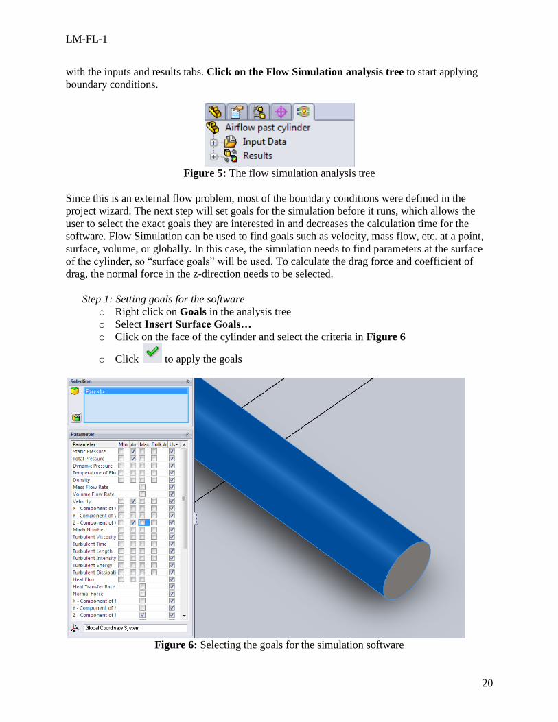
with the inputs and results tabs. Click on the Flow Simulation analysis tree to start applying
boundary conditions.
Figure 5: The flow simulation analysis tree
Since this is an external flow problem, most of the boundary conditions were defined in the
project wizard. The next step will set goals for the simulation before it runs, which allows the
user to select the exact goals they are interested in and decreases the calculation time for the
software. Flow Simulation can be used to find goals such as velocity, mass flow, etc. at a point,
surface, volume, or globally. In this case, the simulation needs to find parameters at the surface
of the cylinder, so “surface goals” will be used. To calculate the drag force and coefficient of
drag, the normal force in the z-direction needs to be selected.
Step 1: Setting goals for the software
o Right click on Goals in the analysis tree
o Select Insert Surface Goals…
o Click on the face of the cylinder and select the criteria in Figure 6
o Click to apply the goals
Figure 6: Selecting the goals for the simulation software
LM-FL-1
21
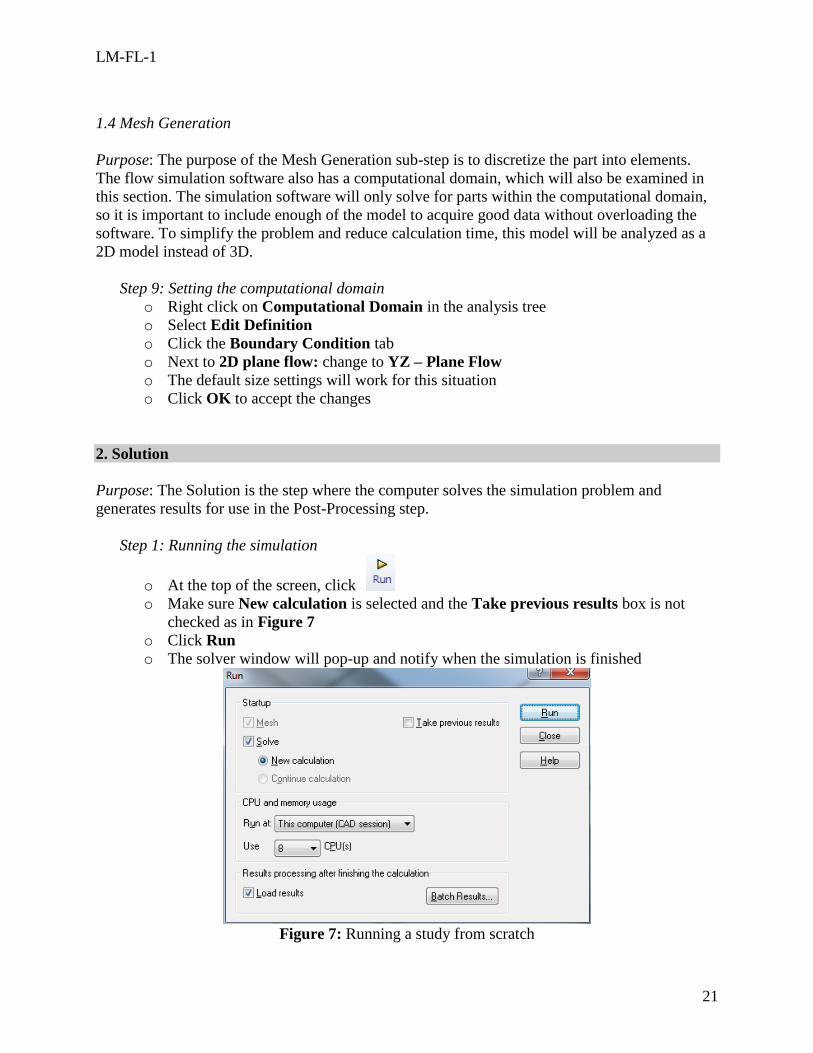
1.4 Mesh Generation
Purpose: The purpose of the Mesh Generation sub-step is to discretize the part into elements.
The flow simulation software also has a computational domain, which will also be examined in
this section. The simulation software will only solve for parts within the computational domain,
so it is important to include enough of the model to acquire good data without overloading the
software. To simplify the problem and reduce calculation time, this model will be analyzed as a
2D model instead of 3D.
Step 9: Setting the computational domain
o Right click on Computational Domain in the analysis tree
o Select Edit Definition
o Click the Boundary Condition tab
o Next to 2D plane flow: change to YZ – Plane Flow
o The default size settings will work for this situation
o Click OK to accept the changes
2. Solution
Purpose: The Solution is the step where the computer solves the simulation problem and
generates results for use in the Post-Processing step.
Step 1: Running the simulation
o At the top of the screen, click
o Make sure New calculation is selected and the Take previous results box is not
checked as in Figure 7
o Click Run
o The solver window will pop-up and notify when the simulation is finished
Figure 7: Running a study from scratch
LM-FL-1
22
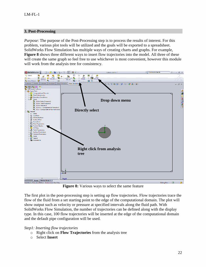
3. Post-Processing
Purpose: The purpose of the Post-Processing step is to process the results of interest. For this
problem, various plot tools will be utilized and the goals will be exported to a spreadsheet.
SolidWorks Flow Simulation has multiple ways of creating charts and graphs. For example,
Figure 8 shows three different ways to insert flow trajectories into the model. All three of these
will create the same graph so feel free to use whichever is most convenient, however this module
will work from the analysis tree for consistency.
Figure 8: Various ways to select the same feature
The first plot in the post-processing step is setting up flow trajectories. Flow trajectories trace the
flow of the fluid from a set starting point to the edge of the computational domain. The plot will
show output such as velocity or pressure at specified intervals along the fluid path. With
SolidWorks Flow Simulation, the number of trajectories can be defined along with the display
type. In this case, 100 flow trajectories will be inserted at the edge of the computational domain
and the default pipe configuration will be used.
Step1: Inserting flow trajectories
o Right click on Flow Trajectories from the analysis tree
o Select Insert
Drop down menu
Directly select
Right click from analysis
tree
LM-FL-1
23
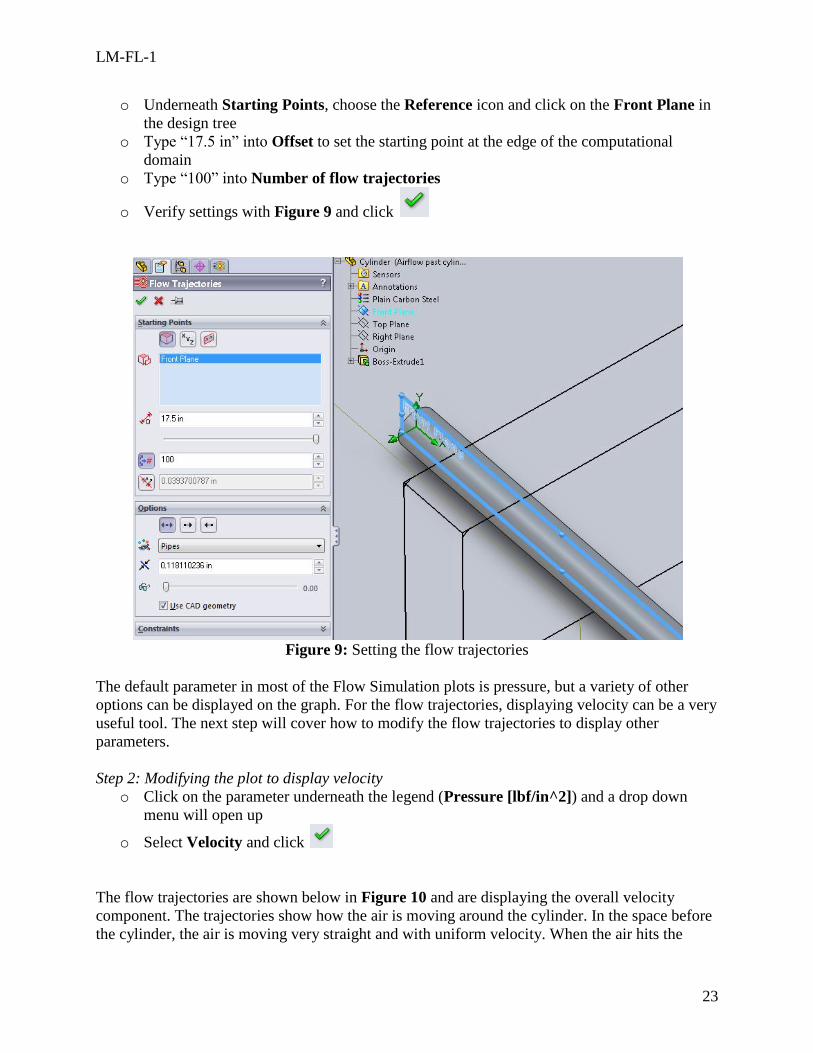
o Underneath Starting Points, choose the Reference icon and click on the Front Plane in
the design tree
o Type “17.5 in” into Offset to set the starting point at the edge of the computational
domain
o Type “100” into Number of flow trajectories
o Verify settings with Figure 9 and click
Figure 9: Setting the flow trajectories
The default parameter in most of the Flow Simulation plots is pressure, but a variety of other
options can be displayed on the graph. For the flow trajectories, displaying velocity can be a very
useful tool. The next step will cover how to modify the flow trajectories to display other
parameters.
Step 2: Modifying the plot to display velocity
o Click on the parameter underneath the legend (Pressure [lbf/in^2]) and a drop down
menu will open up
o Select Velocity and click
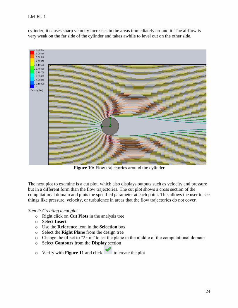
The flow trajectories are shown below in Figure 10 and are displaying the overall velocity
component. The trajectories show how the air is moving around the cylinder. In the space before
the cylinder, the air is moving very straight and with uniform velocity. When the air hits the
LM-FL-1
24
cylinder, it causes sharp velocity increases in the areas immediately around it. The airflow is
very weak on the far side of the cylinder and takes awhile to level out on the other side.
Figure 10: Flow trajectories around the cylinder
The next plot to examine is a cut plot, which also displays outputs such as velocity and pressure
but in a different form than the flow trajectories. The cut plot shows a cross section of the
computational domain and plots the specified parameter at each point. This allows the user to see
things like pressure, velocity, or turbulence in areas that the flow trajectories do not cover.
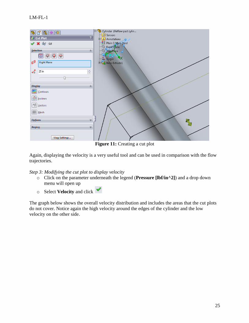
Step 2: Creating a cut plot
o Right click on Cut Plots in the analysis tree
o Select Insert
o Use the Reference icon in the Selection box
o Select the Right Plane from the design tree
o Change the offset to “25 in” to set the plane in the middle of the computational domain
o Select Contours from the Display section
o Verify with Figure 11 and click to create the plot
LM-FL-1
25
Figure 11: Creating a cut plot
Again, displaying the velocity is a very useful tool and can be used in comparison with the flow
trajectories.
Step 3: Modifying the cut plot to display velocity
o Click on the parameter underneath the legend (Pressure [lbf/in^2]) and a drop down
menu will open up
o Select Velocity and click
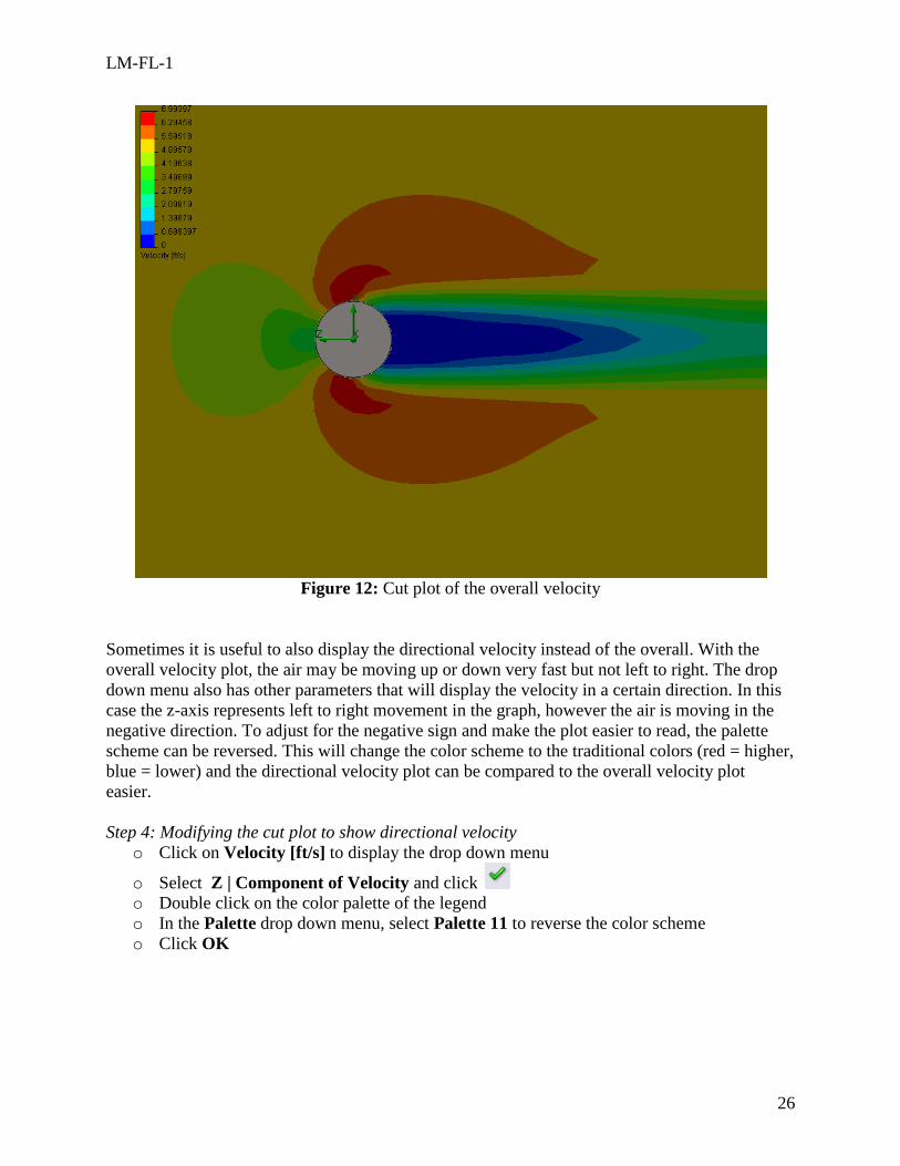
The graph below shows the overall velocity distribution and includes the areas that the cut plots
do not cover. Notice again the high velocity around the edges of the cylinder and the low
velocity on the other side.
LM-FL-1
26
Figure 12: Cut plot of the overall velocity
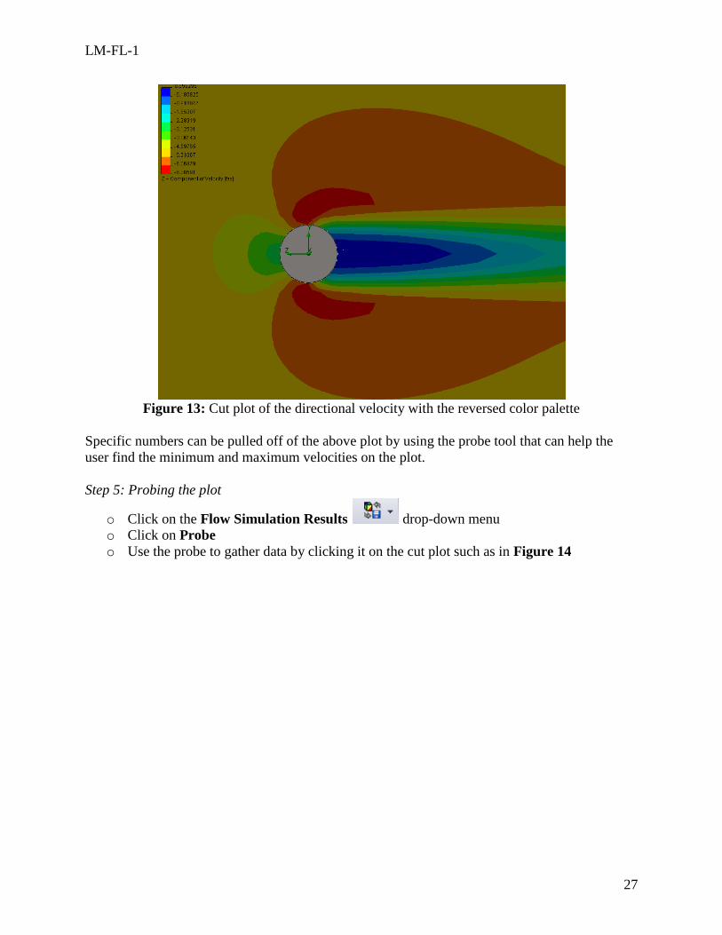
Sometimes it is useful to also display the directional velocity instead of the overall. With the
overall velocity plot, the air may be moving up or down very fast but not left to right. The drop
down menu also has other parameters that will display the velocity in a certain direction. In this
case the z-axis represents left to right movement in the graph, however the air is moving in the
negative direction. To adjust for the negative sign and make the plot easier to read, the palette
scheme can be reversed. This will change the color scheme to the traditional colors (red = higher,
blue = lower) and the directional velocity plot can be compared to the overall velocity plot
easier.
Step 4: Modifying the cut plot to show directional velocity
o Click on Velocity [ft/s] to display the drop down menu
o Select Z | Component of Velocity and click
o Double click on the color palette of the legend
o In the Palette drop down menu, select Palette 11 to reverse the color scheme
o Click OK
LM-FL-1
27
Figure 13: Cut plot of the directional velocity with the reversed color palette
Specific numbers can be pulled off of the above plot by using the probe tool that can help the
user find the minimum and maximum velocities on the plot.
Step 5: Probing the plot
o Click on the Flow Simulation Results drop-down menu
o Click on Probe
o Use the probe to gather data by clicking it on the cut plot such as in Figure 14
LM-FL-1
28
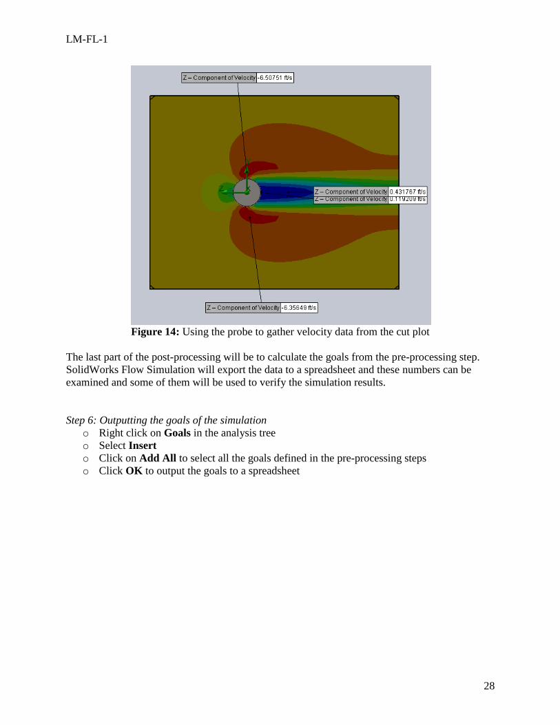
Figure 14: Using the probe to gather velocity data from the cut plot
The last part of the post-processing will be to calculate the goals from the pre-processing step.
SolidWorks Flow Simulation will export the data to a spreadsheet and these numbers can be
examined and some of them will be used to verify the simulation results.
Step 6: Outputting the goals of the simulation
o Right click on Goals in the analysis tree
o Select Insert
o Click on Add All to select all the goals defined in the pre-processing steps
o Click OK to output the goals to a spreadsheet
LM-FL-1
29
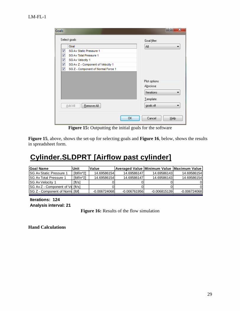
Figure 15: Outputting the initial goals for the software
Figure 15, above, shows the set-up for selecting goals and Figure 16, below, shows the results
in spreadsheet form.
Figure 16: Results of the flow simulation
Hand Calculations
Cylinder.SLDPRT [Airflow past cylinder]
Goal Name Unit Value Averaged Value Minimum Value Maximum Value Progress [%] Use In Convergence Delta Criteria
SG Av Static Pressure 1 [lbf/in 2] 14.69586154 14.69586147 14.69586143 14.69586154 100 Yes 1.04373E-07 2.74449E-06
SG Av Total Pressure 1 [lbf/in 2] 14.69586154 14.69586147 14.69586143 14.69586154 100 Yes 1.04373E-07 2.74449E-06
SG Av Velocity 1 [ft/s] 0 0 0 0 100 Yes 0 0
SG Av Z - Component of Velocity 1 [ft/s] 0 0 0 0 100 Yes 0 0
SG Z - Component of Normal Force 1 [lbf] -0.006724068 -0.006761956 -0.006815139 -0.006724068 100 Yes 9.1071E-05 9.37704E-05
Iterations: 124
Analysis interval: 21

LM-FL-1
30
Attachment C1. SolidWorks-Specific FEM Tutorial 2
Overview: In this section, three tutorial problems will be solved using the commercial FEM
software SolidWorks. Although the underlying principles and logical steps of an FEM simulation
identified in the Conceptual Analysis section are independent of any particular FEM software,
the realization of conceptual analysis steps will be software dependent. The SolidWorks-specific
steps are described in this section.
This is a step-by-step tutorial. However, it is designed such that those who are familiar with the
details in a particular step can skip it and go directly into the next step.
Tutorial Problem 1.
1. Launching SolidWorks
SolidWorks Simulation is an integral part of the SolidWorks computer aided design software
suite. The general user interface of SolidWorks is shown in Figure 1.
Figure 1: General user interface of SolidWorks.
In order to perform flow analysis, it is necessary to enable the software add-in component, called
SolidWorks Flow Simulation.
Main menu Frequently used command icons Help icon
Roll over to
display
“File”,
“Tools” and
other menus

LM-FL-1
31
Step 1: Enabling SolidWorks Flow Simulation
o Click Tools in the main menu and select Add-ins.... The Add-ins dialog window
appears, as shown in Figure 2.
o Check the boxes in both the Active Add-ins and Start Up columns corresponding to
SolidWorks Flow Simulation.
o Checking the Active Add-ins box enables SolidWorks to activate the Flow
Simulation package for the current session. Checking the Start Up box enables the
Flow Simulation package for all future sessions whenever SolidWorks starts up.
Figure 2: Location of the SolidWorks icon and the boxes to be checked for adding it to the
panel.
1. Pre-Processing
Purpose: The purpose of pre-processing is to create an FEM model for use in the next step of the
simulation, Solution. It consists of the following sub-steps:
Geometry creation
Material property assignment
Boundary condition specification
Mesh generation.
LM-FL-1
32
1.1 Geometry Creation
The purpose of Geometry Creation is to create a geometrical representation of the solid object or
structure to be analyzed. In SolidWorks, such a geometric model is called a part. In this tutorial,
the necessary part has already been created in SolidWorks. The following steps will open up the
part for use in the flow analysis.
Step 1: Opening the part for simulation. One of the following two options can be used.
o Option1: Double click the following icon to open the embedded part file,
Room.SLDPRT, in SolidWorks
Click SolidWorks part file icon to open it ==>
o Option 2: Download the part file “Room.SLDPRT” from the web site
http://www.femlearning.org/. Use the File menu in SolidWorks to open the
downloaded part.
The SolidWorks model tree will appear with the given part name at the top. Above the model
tree, there should be various tabs labeled Features, Sketch, etc. If the Flow Simulation tab is
not visible, go back to steps 1 and 2 to enable the SolidWorks Flow Simulation package.
SolidWorks Flow Simulation has two options to create a new project: using the configuration
wizard and creating a new project with default settings. In this situation, the project configuration
will be used to specify the initial conditions.
This tutorial problem is an internal analysis so the set-up is slightly different from the previous
example. The initial velocity and pressure conditions will be specified by using the flow analysis
tree instead of the project wizard.
Step 2: Using the flow simulation wizard to configure a new project
o Click the tab above the model tree
o Click the icon to create a new flow simulation study
o In the first step of the wizard, select Create new and type “Airflow through room”
next to Configuration name and click Next >
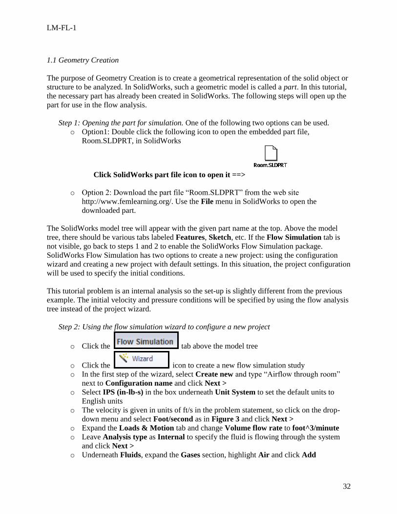
o Select IPS (in-lb-s) in the box underneath Unit System to set the default units to
English units
o The velocity is given in units of ft/s in the problem statement, so click on the drop-
down menu and select Foot/second as in Figure 3 and click Next >
o Expand the Loads & Motion tab and change Volume flow rate to foot^3/minute
o Leave Analysis type as Internal to specify the fluid is flowing through the system
and click Next >
o Underneath Fluids, expand the Gases section, highlight Air and click Add
LM-FL-1
33
o Once Air (Gases) is added to the Project Fluids and the Default Fluid box is
checked, click Next >
o Leave the Default wall thermal condition as “Adiabatic wall” and Roughness at “0
microinch” and click Next >
o Use the default settings for initial conditions and click Next>
o Click Next > and then Finish to complete the set-up
Figure 3: Specifying units for flow analysis
1.2 Material Property Assignment
The next step in FEM analysis is to apply the material properties to the cylinder. For simplicity,
the entire room will be modeled with a 1060 Aluminum alloy.
Step 1: Applying the material
o Right click on the Room part in the model tree
o Select Material -> Edit material
o Expand the Aluminum Alloys section and select 1060
LM-FL-1
34
o Click Apply to accept the changes and Close
1.3 Boundary Condition Specification
Purpose: The purpose of this section is apply the correct boundary conditions and set goals for
the simulation software. SolidWorks Flow Simulation has many ways to apply boundary
conditions to a model. Many of the icons that will be used in this module are under the Flow
Simulation tab in the command manager and can also be found by clicking on the Flow
Simulation analysis tree.
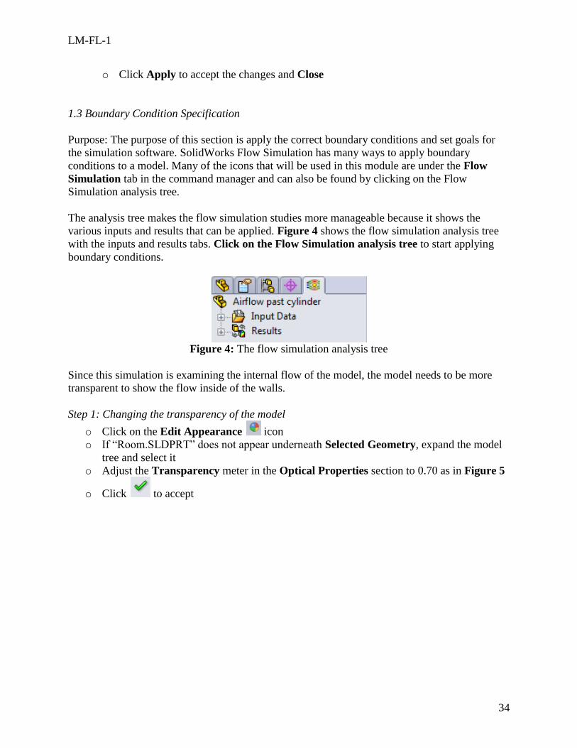
The analysis tree makes the flow simulation studies more manageable because it shows the
various inputs and results that can be applied. Figure 4 shows the flow simulation analysis tree
with the inputs and results tabs. Click on the Flow Simulation analysis tree to start applying
boundary conditions.
Figure 4: The flow simulation analysis tree
Since this simulation is examining the internal flow of the model, the model needs to be more
transparent to show the flow inside of the walls.
Step 1: Changing the transparency of the model
o Click on the Edit Appearance icon
o If “Room.SLDPRT” does not appear underneath Selected Geometry, expand the model
tree and select it
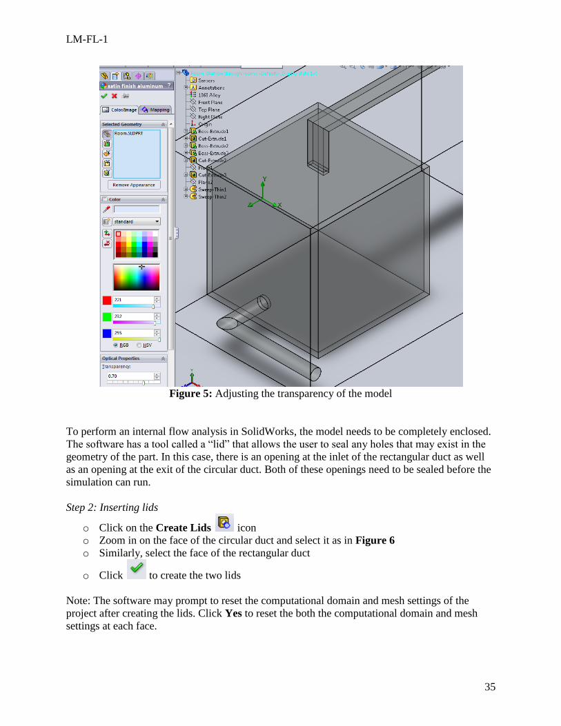
o Adjust the Transparency meter in the Optical Properties section to 0.70 as in Figure 5
o Click to accept
LM-FL-1
35
Figure 5: Adjusting the transparency of the model
To perform an internal flow analysis in SolidWorks, the model needs to be completely enclosed.
The software has a tool called a “lid” that allows the user to seal any holes that may exist in the
geometry of the part. In this case, there is an opening at the inlet of the rectangular duct as well
as an opening at the exit of the circular duct. Both of these openings need to be sealed before the
simulation can run.
Step 2: Inserting lids
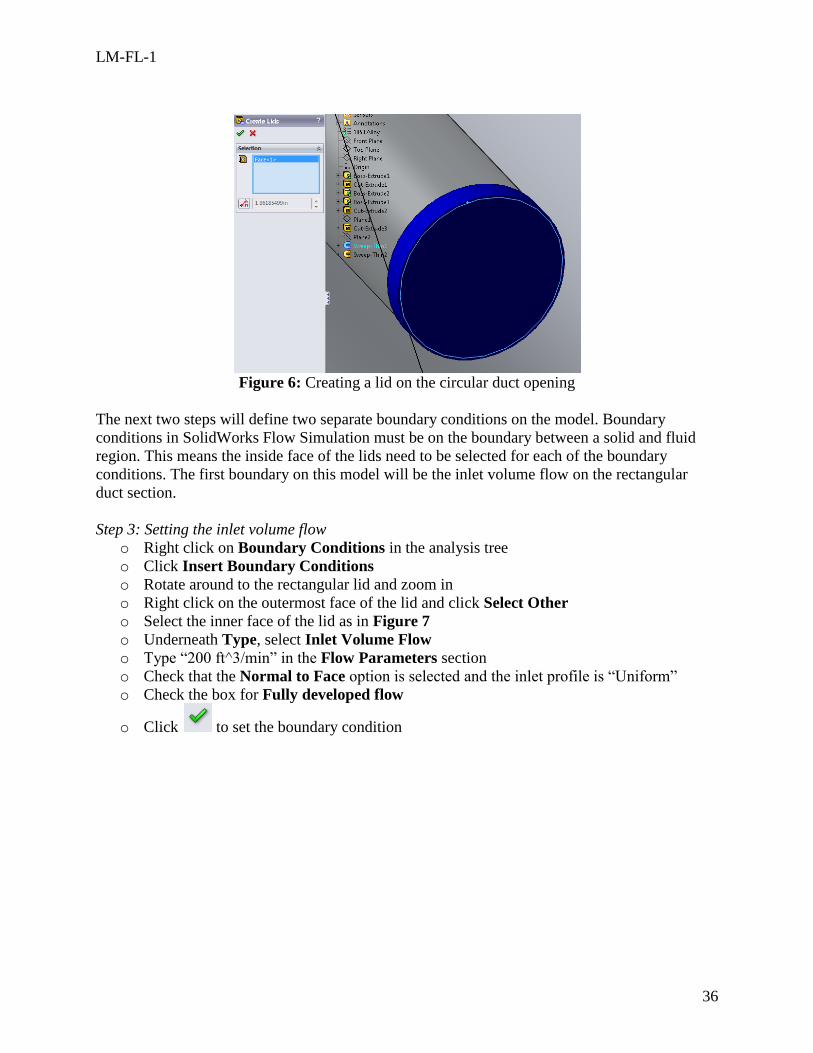
o Click on the Create Lids icon
o Zoom in on the face of the circular duct and select it as in Figure 6
o Similarly, select the face of the rectangular duct
o Click to create the two lids
Note: The software may prompt to reset the computational domain and mesh settings of the
project after creating the lids. Click Yes to reset the both the computational domain and mesh
settings at each face.
LM-FL-1
36
Figure 6: Creating a lid on the circular duct opening
The next two steps will define two separate boundary conditions on the model. Boundary
conditions in SolidWorks Flow Simulation must be on the boundary between a solid and fluid
region. This means the inside face of the lids need to be selected for each of the boundary
conditions. The first boundary on this model will be the inlet volume flow on the rectangular
duct section.
Step 3: Setting the inlet volume flow
o Right click on Boundary Conditions in the analysis tree
o Click Insert Boundary Conditions
o Rotate around to the rectangular lid and zoom in
o Right click on the outermost face of the lid and click Select Other
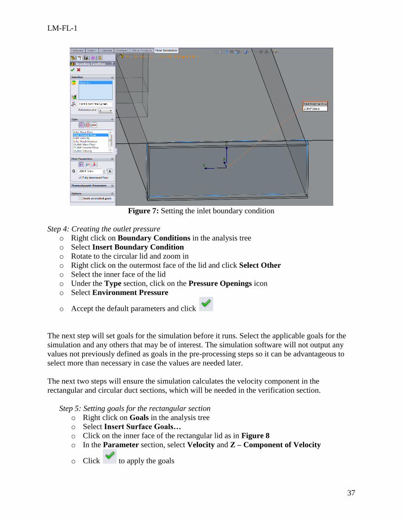
o Select the inner face of the lid as in Figure 7
o Underneath Type, select Inlet Volume Flow
o Type “200 ft^3/min” in the Flow Parameters section
o Check that the Normal to Face option is selected and the inlet profile is “Uniform”
o Check the box for Fully developed flow
o Click to set the boundary condition
LM-FL-1
37
Figure 7: Setting the inlet boundary condition
Step 4: Creating the outlet pressure
o Right click on Boundary Conditions in the analysis tree
o Select Insert Boundary Condition
o Rotate to the circular lid and zoom in
o Right click on the outermost face of the lid and click Select Other
o Select the inner face of the lid
o Under the Type section, click on the Pressure Openings icon
o Select Environment Pressure
o Accept the default parameters and click
The next step will set goals for the simulation before it runs. Select the applicable goals for the
simulation and any others that may be of interest. The simulation software will not output any
values not previously defined as goals in the pre-processing steps so it can be advantageous to
select more than necessary in case the values are needed later.
The next two steps will ensure the simulation calculates the velocity component in the
rectangular and circular duct sections, which will be needed in the verification section.
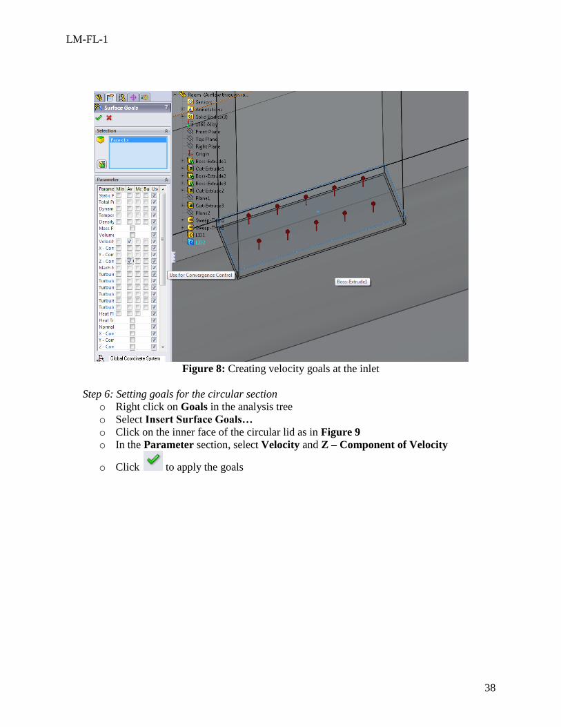
Step 5: Setting goals for the rectangular section
o Right click on Goals in the analysis tree
o Select Insert Surface Goals…
o Click on the inner face of the rectangular lid as in Figure 8
o In the Parameter section, select Velocity and Z – Component of Velocity
o Click to apply the goals
LM-FL-1
38
Figure 8: Creating velocity goals at the inlet
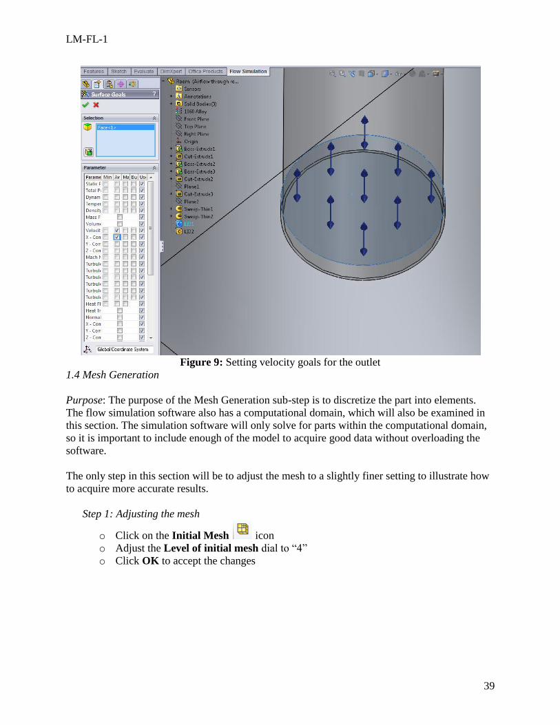
Step 6: Setting goals for the circular section
o Right click on Goals in the analysis tree
o Select Insert Surface Goals…
o Click on the inner face of the circular lid as in Figure 9
o In the Parameter section, select Velocity and Z – Component of Velocity
o Click to apply the goals
LM-FL-1
39
Figure 9: Setting velocity goals for the outlet
1.4 Mesh Generation
Purpose: The purpose of the Mesh Generation sub-step is to discretize the part into elements.
The flow simulation software also has a computational domain, which will also be examined in
this section. The simulation software will only solve for parts within the computational domain,
so it is important to include enough of the model to acquire good data without overloading the
software.
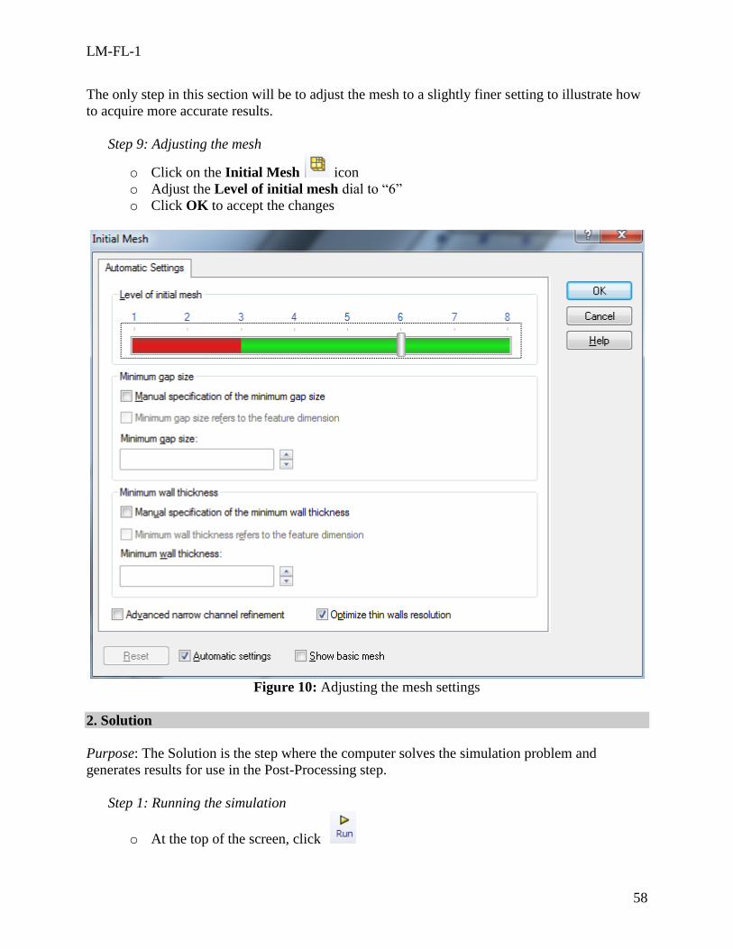
The only step in this section will be to adjust the mesh to a slightly finer setting to illustrate how
to acquire more accurate results.
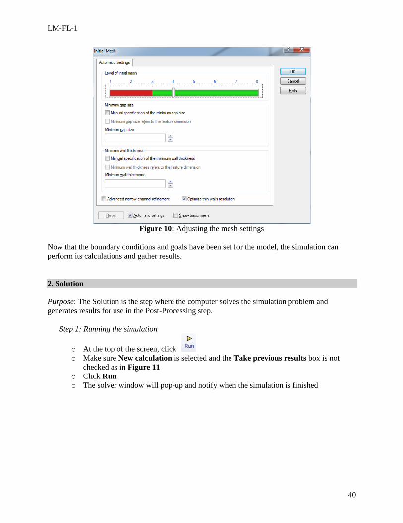
Step 1: Adjusting the mesh
o Click on the Initial Mesh icon
o Adjust the Level of initial mesh dial to “4”
o Click OK to accept the changes
LM-FL-1
40
Figure 10: Adjusting the mesh settings
Now that the boundary conditions and goals have been set for the model, the simulation can
perform its calculations and gather results.
2. Solution
Purpose: The Solution is the step where the computer solves the simulation problem and
generates results for use in the Post-Processing step.
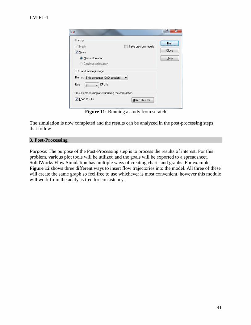
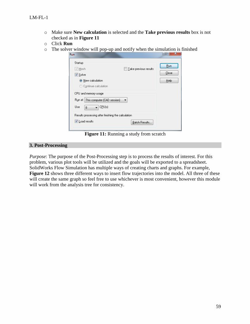
Step 1: Running the simulation
o At the top of the screen, click
o Make sure New calculation is selected and the Take previous results box is not
checked as in Figure 11
o Click Run
o The solver window will pop-up and notify when the simulation is finished
LM-FL-1
41
Figure 11: Running a study from scratch
The simulation is now completed and the results can be analyzed in the post-processing steps
that follow.
3. Post-Processing
Purpose: The purpose of the Post-Processing step is to process the results of interest. For this
problem, various plot tools will be utilized and the goals will be exported to a spreadsheet.
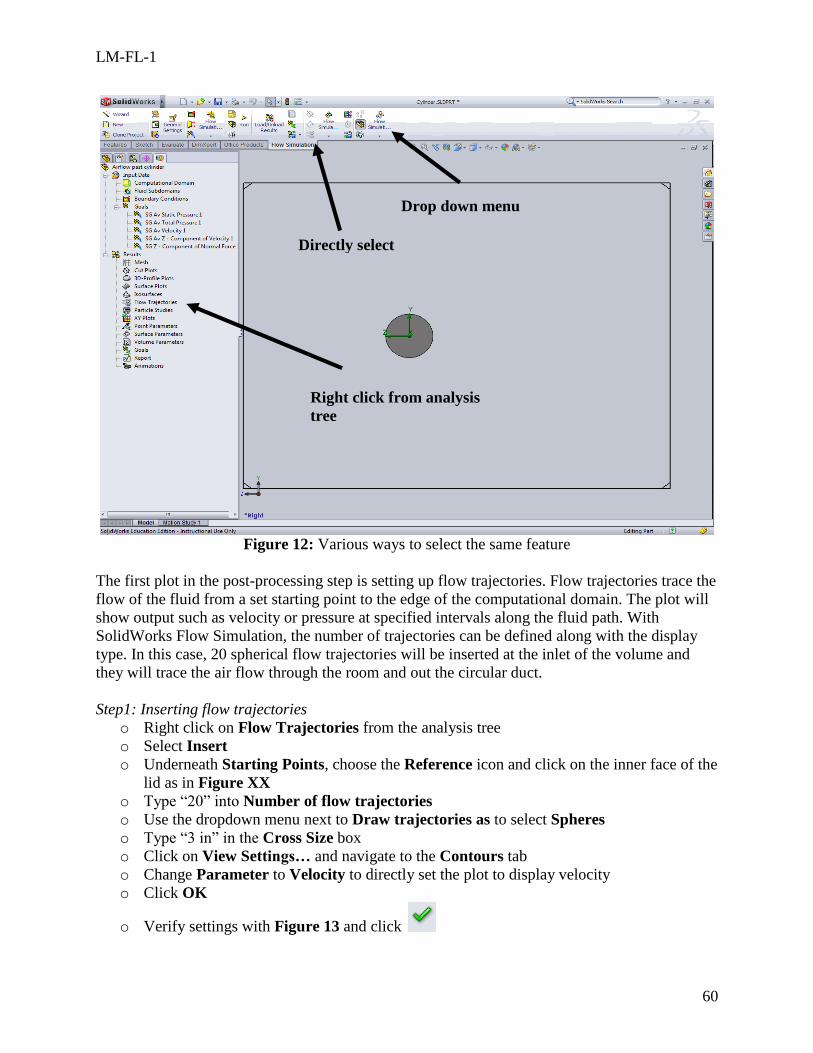
SolidWorks Flow Simulation has multiple ways of creating charts and graphs. For example,
Figure 12 shows three different ways to insert flow trajectories into the model. All three of these
will create the same graph so feel free to use whichever is most convenient, however this module
will work from the analysis tree for consistency.
LM-FL-1
42
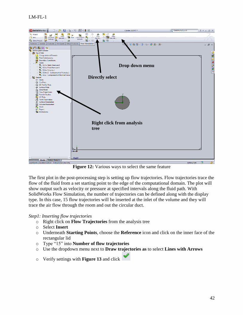
Figure 12: Various ways to select the same feature
The first plot in the post-processing step is setting up flow trajectories. Flow trajectories trace the
flow of the fluid from a set starting point to the edge of the computational domain. The plot will
show output such as velocity or pressure at specified intervals along the fluid path. With
SolidWorks Flow Simulation, the number of trajectories can be defined along with the display
type. In this case, 15 flow trajectories will be inserted at the inlet of the volume and they will
trace the air flow through the room and out the circular duct.
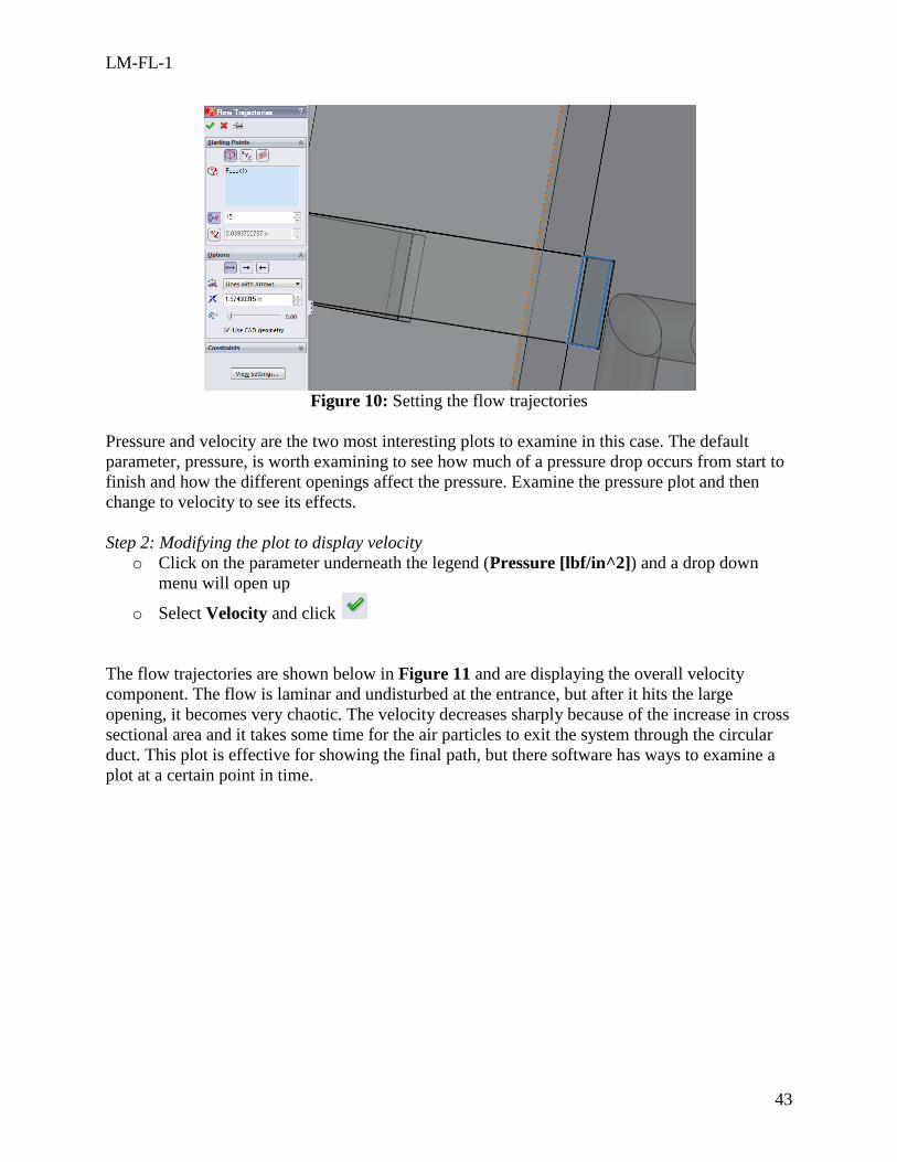
Step1: Inserting flow trajectories
o Right click on Flow Trajectories from the analysis tree
o Select Insert
o Underneath Starting Points, choose the Reference icon and click on the inner face of the
rectangular lid
o Type “15” into Number of flow trajectories
o Use the dropdown menu next to Draw trajectories as to select Lines with Arrows
o Verify settings with Figure 13 and click
Drop down menu
Directly select
Right click from analysis
tree
LM-FL-1
43
Figure 10: Setting the flow trajectories
Pressure and velocity are the two most interesting plots to examine in this case. The default
parameter, pressure, is worth examining to see how much of a pressure drop occurs from start to
finish and how the different openings affect the pressure. Examine the pressure plot and then
change to velocity to see its effects.
Step 2: Modifying the plot to display velocity
o Click on the parameter underneath the legend (Pressure [lbf/in^2]) and a drop down
menu will open up
o Select Velocity and click
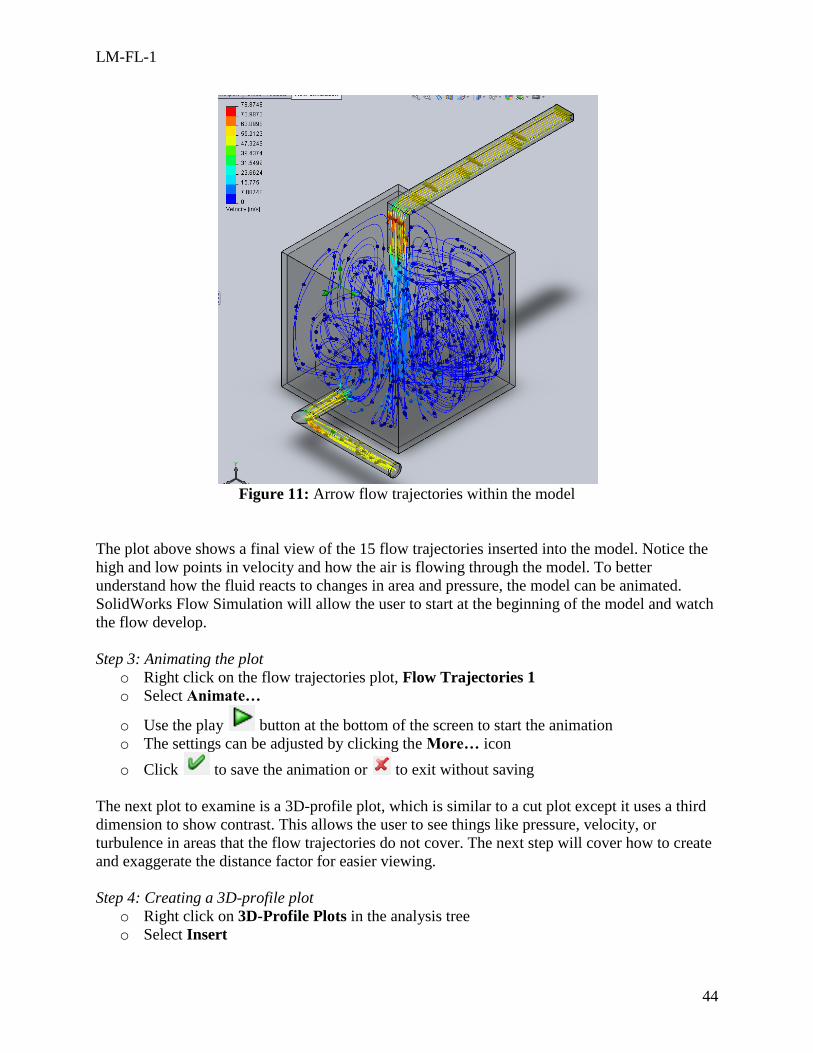
The flow trajectories are shown below in Figure 11 and are displaying the overall velocity
component. The flow is laminar and undisturbed at the entrance, but after it hits the large
opening, it becomes very chaotic. The velocity decreases sharply because of the increase in cross
sectional area and it takes some time for the air particles to exit the system through the circular
duct. This plot is effective for showing the final path, but there software has ways to examine a
plot at a certain point in time.
LM-FL-1
44
Figure 11: Arrow flow trajectories within the model
The plot above shows a final view of the 15 flow trajectories inserted into the model. Notice the
high and low points in velocity and how the air is flowing through the model. To better
understand how the fluid reacts to changes in area and pressure, the model can be animated.
SolidWorks Flow Simulation will allow the user to start at the beginning of the model and watch
the flow develop.
Step 3: Animating the plot
o Right click on the flow trajectories plot, Flow Trajectories 1
o Select Animate…
o Use the play button at the bottom of the screen to start the animation
o The settings can be adjusted by clicking the More… icon
o Click to save the animation or to exit without saving
The next plot to examine is a 3D-profile plot, which is similar to a cut plot except it uses a third
dimension to show contrast. This allows the user to see things like pressure, velocity, or
turbulence in areas that the flow trajectories do not cover. The next step will cover how to create
and exaggerate the distance factor for easier viewing.
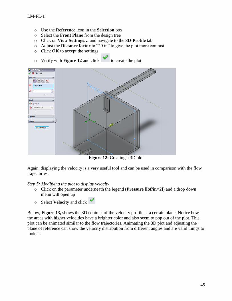
Step 4: Creating a 3D-profile plot
o Right click on 3D-Profile Plots in the analysis tree
o Select Insert
LM-FL-1
45
o Use the Reference icon in the Selection box
o Select the Front Plane from the design tree
o Click on View Settings… and navigate to the 3D-Profile tab
o Adjust the Distance factor to “20 in” to give the plot more contrast
o Click OK to accept the settings
o Verify with Figure 12 and click to create the plot
Figure 12: Creating a 3D plot
Again, displaying the velocity is a very useful tool and can be used in comparison with the flow
trajectories.
Step 5: Modifying the plot to display velocity
o Click on the parameter underneath the legend (Pressure [lbf/in^2]) and a drop down
menu will open up
o Select Velocity and click
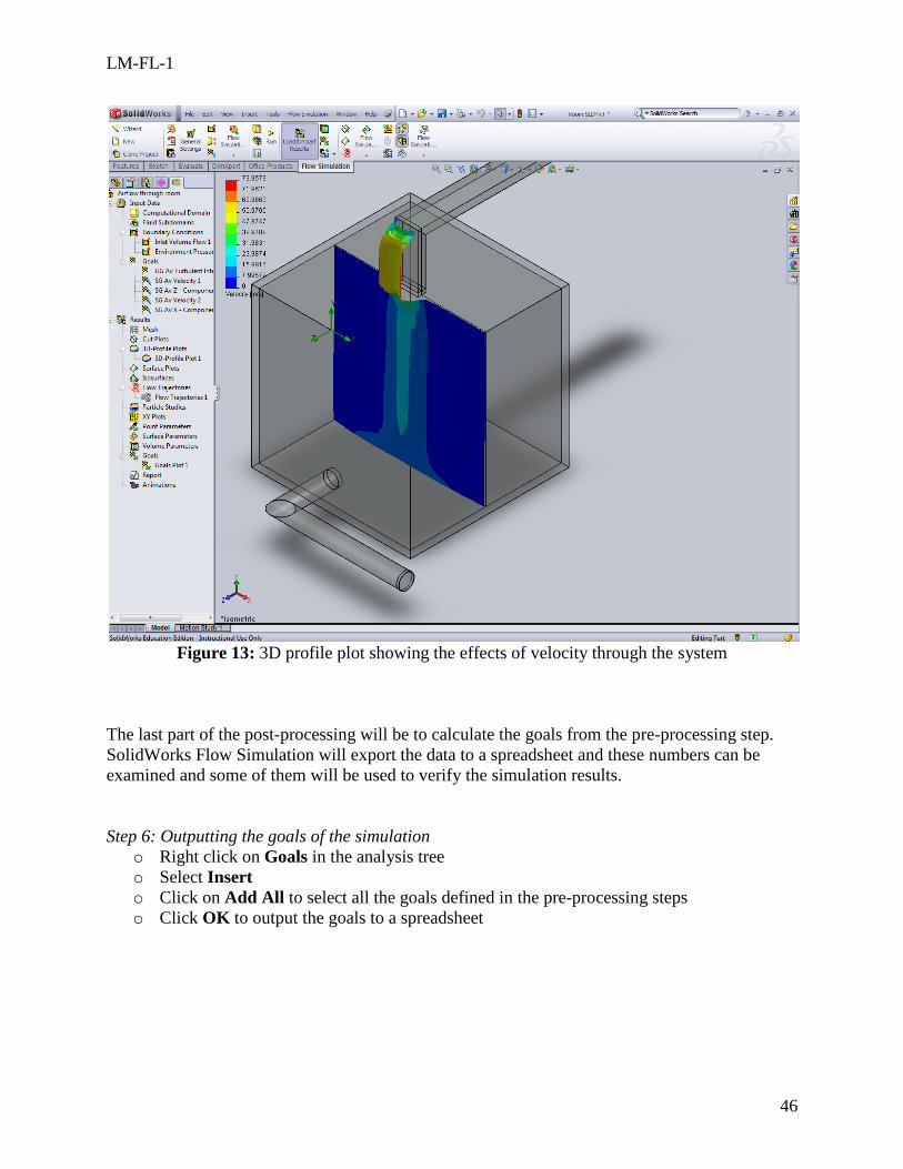
Below, Figure 13, shows the 3D contrast of the velocity profile at a certain plane. Notice how
the areas with higher velocities have a brighter color and also seem to pop out of the plot. This
plot can be animated similar to the flow trajectories. Animating the 3D plot and adjusting the
plane of reference can show the velocity distribution from different angles and are valid things to
look at.
LM-FL-1
46
Figure 13: 3D profile plot showing the effects of velocity through the system
The last part of the post-processing will be to calculate the goals from the pre-processing step.
SolidWorks Flow Simulation will export the data to a spreadsheet and these numbers can be
examined and some of them will be used to verify the simulation results.
Step 6: Outputting the goals of the simulation
o Right click on Goals in the analysis tree
o Select Insert
o Click on Add All to select all the goals defined in the pre-processing steps
o Click OK to output the goals to a spreadsheet
LM-FL-1
47
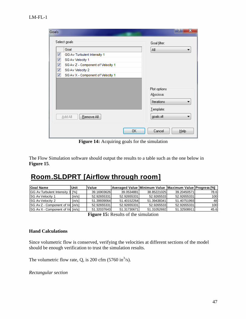
Figure 14: Acquiring goals for the simulation
The Flow Simulation software should output the results to a table such as the one below in
Figure 15.
Figure 15: Results of the simulation
Hand Calculations
Since volumetric flow is conserved, verifying the velocities at different sections of the model
should be enough verification to trust the simulation results.
The volumetric flow rate, Q, is 200 cfm (5760 in3/s).
Rectangular section
Room.SLDPRT [Airflow through room]
Goal Name Unit Value Averaged Value Minimum Value Maximum Value Progress [%]
GG Av Turbulent Intensity 1 [%] 39.16903626 39.0534881 38.85221025 39.20450571 78.6
SG Av Velocity 1 [in/s] 52.92655331 52.92655331 52.9265533 52.92655331 100
SG Av Velocity 2 [in/s] 51.39939064 51.40152264 51.39438341 51.40751993 48
SG Av Z - Component of Velocity 1 [in/s] 52.92655331 52.92655331 52.9265533 52.92655331 100
SG Av X - Component of Velocity 1 [in/s] 51.32037643 51.31730671 51.31052692 51.32508911 45.6
LM-FL-1
48
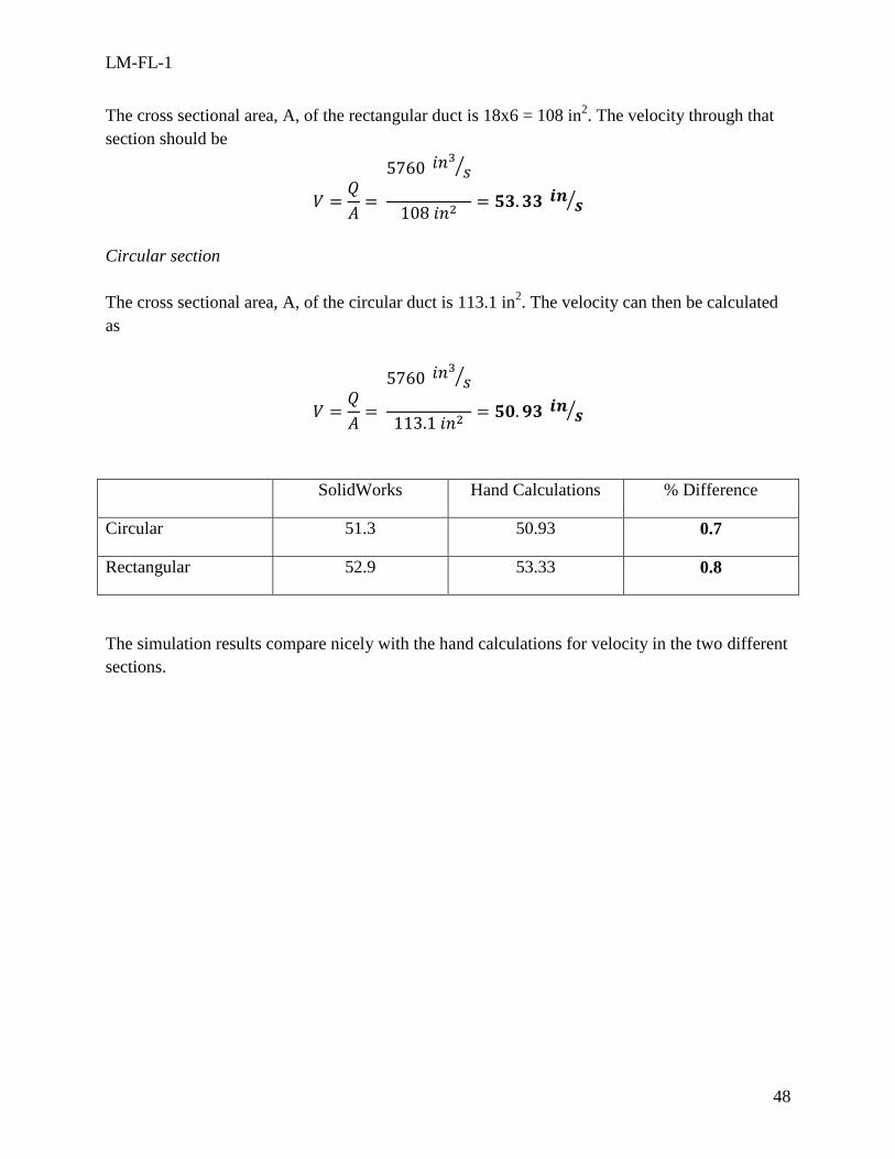
The cross sectional area, A, of the rectangular duct is 18x6 = 108 in2. The velocity through that
section should be
⁄
⁄
Circular section
The cross sectional area, A, of the circular duct is 113.1 in2. The velocity can then be calculated
as
⁄
⁄
SolidWorks Hand Calculations % Difference
Circular 51.3 50.93 0.7
Rectangular 52.9 53.33 0.8
The simulation results compare nicely with the hand calculations for velocity in the two different
sections.
LM-FL-1
49
Attachment C1. SolidWorks-Specific FEM Tutorial 3
Overview: In this section, three tutorial problems will be solved using the commercial FEM
software SolidWorks. Although the underlying principles and logical steps of an FEM simulation
identified in the Conceptual Analysis section are independent of any particular FEM software,
the realization of conceptual analysis steps will be software dependent. The SolidWorks-specific
steps are described in this section.
This is a step-by-step tutorial. However, it is designed such that those who are familiar with the
details in a particular step can skip it and go directly into the next step.
Tutorial Problem 1.
2. Launching SolidWorks
SolidWorks Simulation is an integral part of the SolidWorks computer aided design software
suite. The general user interface of SolidWorks is shown in Figure 1.
Figure 1: General user interface of SolidWorks.
In order to perform flow analysis, it is necessary to enable the software add-in component, called
SolidWorks Flow Simulation.
Main menu Frequently used command icons Help icon
Roll over to
display
“File”,
“Tools” and
other menus
LM-FL-1
50
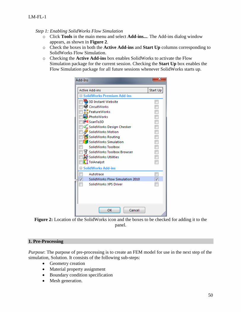
Step 1: Enabling SolidWorks Flow Simulation
o Click Tools in the main menu and select Add-ins.... The Add-ins dialog window
appears, as shown in Figure 2.
o Check the boxes in both the Active Add-ins and Start Up columns corresponding to
SolidWorks Flow Simulation.
o Checking the Active Add-ins box enables SolidWorks to activate the Flow
Simulation package for the current session. Checking the Start Up box enables the
Flow Simulation package for all future sessions whenever SolidWorks starts up.
Figure 2: Location of the SolidWorks icon and the boxes to be checked for adding it to the
panel.
1. Pre-Processing
Purpose: The purpose of pre-processing is to create an FEM model for use in the next step of the
simulation, Solution. It consists of the following sub-steps:
Geometry creation
Material property assignment
Boundary condition specification
Mesh generation.
LM-FL-1
51
1.1 Geometry Creation
The purpose of Geometry Creation is to create a geometrical representation of the solid object or
structure to be analyzed. In SolidWorks, such a geometric model is called a part. In this tutorial,
the necessary part has already been created in SolidWorks. The following steps will open up the
part for use in the flow analysis.
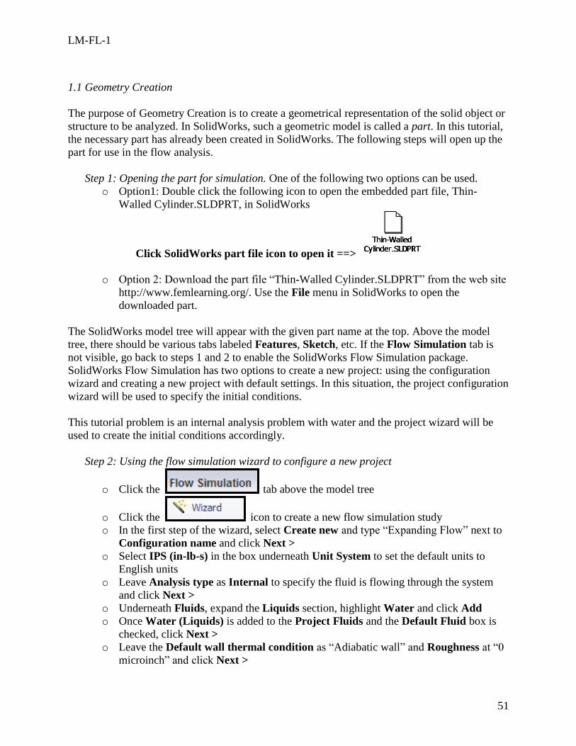
Step 1: Opening the part for simulation. One of the following two options can be used.
o Option1: Double click the following icon to open the embedded part file, Thin-
Walled Cylinder.SLDPRT, in SolidWorks
Click SolidWorks part file icon to open it ==>
o Option 2: Download the part file “Thin-Walled Cylinder.SLDPRT” from the web site
http://www.femlearning.org/. Use the File menu in SolidWorks to open the
downloaded part.
The SolidWorks model tree will appear with the given part name at the top. Above the model
tree, there should be various tabs labeled Features, Sketch, etc. If the Flow Simulation tab is
not visible, go back to steps 1 and 2 to enable the SolidWorks Flow Simulation package.
SolidWorks Flow Simulation has two options to create a new project: using the configuration
wizard and creating a new project with default settings. In this situation, the project configuration
wizard will be used to specify the initial conditions.
This tutorial problem is an internal analysis problem with water and the project wizard will be
used to create the initial conditions accordingly.
Step 2: Using the flow simulation wizard to configure a new project
o Click the tab above the model tree
o Click the icon to create a new flow simulation study
o In the first step of the wizard, select Create new and type “Expanding Flow” next to
Configuration name and click Next >
o Select IPS (in-lb-s) in the box underneath Unit System to set the default units to
English units
o Leave Analysis type as Internal to specify the fluid is flowing through the system
and click Next >
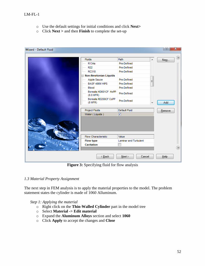
o Underneath Fluids, expand the Liquids section, highlight Water and click Add
o Once Water (Liquids) is added to the Project Fluids and the Default Fluid box is
checked, click Next >
o Leave the Default wall thermal condition as “Adiabatic wall” and Roughness at “0
microinch” and click Next >
LM-FL-1
52
o Use the default settings for initial conditions and click Next>
o Click Next > and then Finish to complete the set-up
Figure 3: Specifying fluid for flow analysis
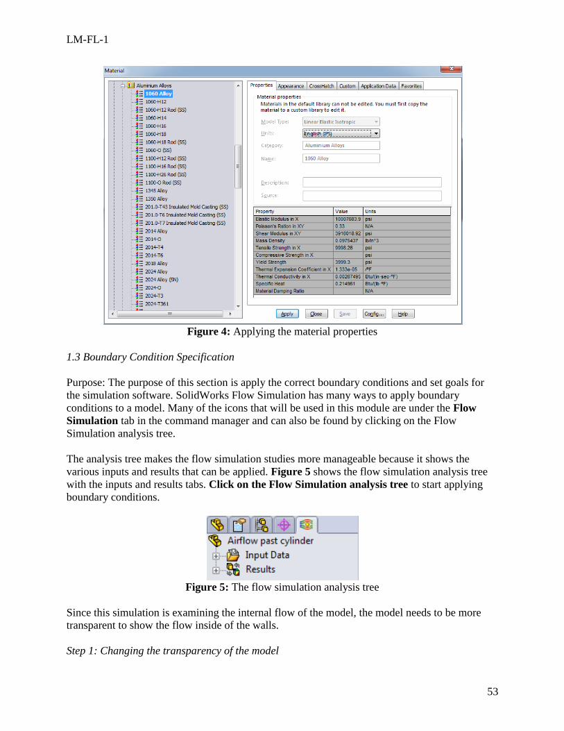
1.3 Material Property Assignment
The next step in FEM analysis is to apply the material properties to the model. The problem
statement states the cylinder is made of 1060 Alluminum.
Step 1: Applying the material
o Right click on the Thin-Walled Cylinder part in the model tree
o Select Material -> Edit material
o Expand the Aluminum Alloys section and select 1060
o Click Apply to accept the changes and Close
LM-FL-1
53
Figure 4: Applying the material properties
1.3 Boundary Condition Specification
Purpose: The purpose of this section is apply the correct boundary conditions and set goals for
the simulation software. SolidWorks Flow Simulation has many ways to apply boundary
conditions to a model. Many of the icons that will be used in this module are under the Flow
Simulation tab in the command manager and can also be found by clicking on the Flow
Simulation analysis tree.
The analysis tree makes the flow simulation studies more manageable because it shows the
various inputs and results that can be applied. Figure 5 shows the flow simulation analysis tree
with the inputs and results tabs. Click on the Flow Simulation analysis tree to start applying
boundary conditions.
Figure 5: The flow simulation analysis tree
Since this simulation is examining the internal flow of the model, the model needs to be more
transparent to show the flow inside of the walls.
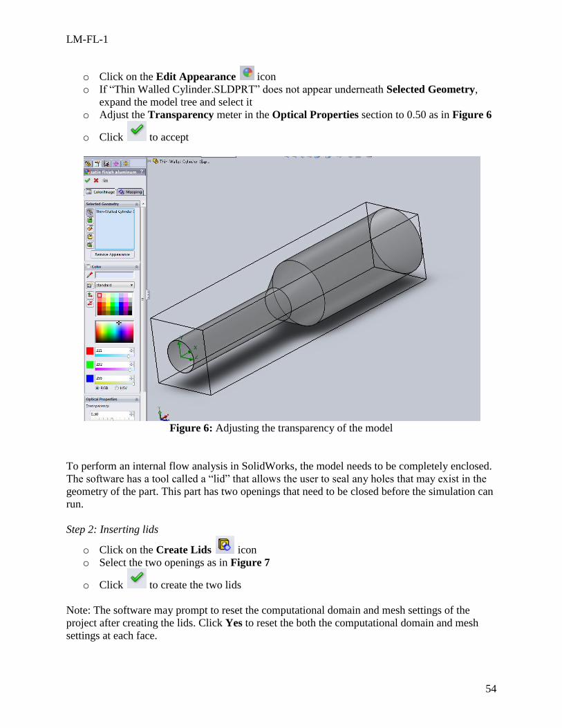
Step 1: Changing the transparency of the model
LM-FL-1
54
o Click on the Edit Appearance icon
o If “Thin Walled Cylinder.SLDPRT” does not appear underneath Selected Geometry,
expand the model tree and select it
o Adjust the Transparency meter in the Optical Properties section to 0.50 as in Figure 6
o Click to accept
Figure 6: Adjusting the transparency of the model
To perform an internal flow analysis in SolidWorks, the model needs to be completely enclosed.
The software has a tool called a “lid” that allows the user to seal any holes that may exist in the
geometry of the part. This part has two openings that need to be closed before the simulation can
run.
Step 2: Inserting lids
o Click on the Create Lids icon
o Select the two openings as in Figure 7
o Click to create the two lids
Note: The software may prompt to reset the computational domain and mesh settings of the
project after creating the lids. Click Yes to reset the both the computational domain and mesh
settings at each face.
LM-FL-1
55
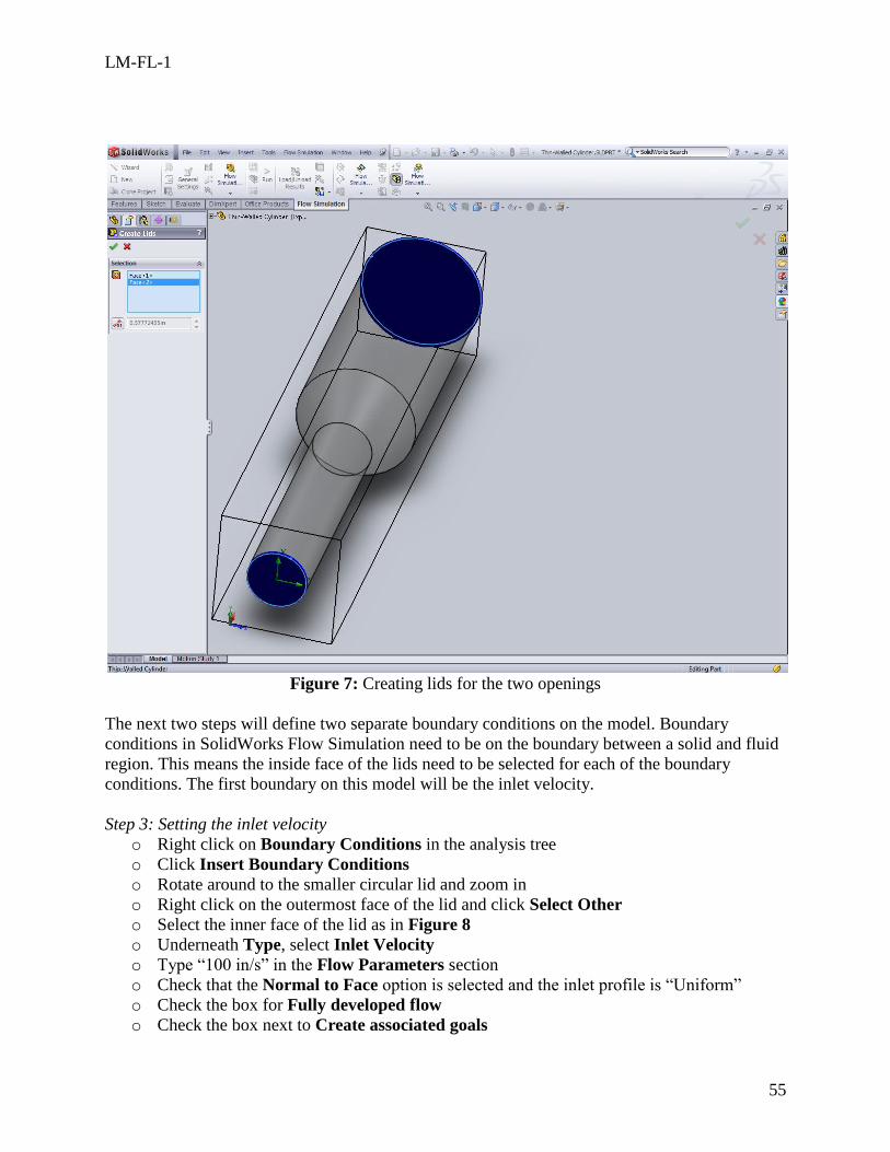
Figure 7: Creating lids for the two openings
The next two steps will define two separate boundary conditions on the model. Boundary
conditions in SolidWorks Flow Simulation need to be on the boundary between a solid and fluid
region. This means the inside face of the lids need to be selected for each of the boundary
conditions. The first boundary on this model will be the inlet velocity.
Step 3: Setting the inlet velocity
o Right click on Boundary Conditions in the analysis tree
o Click Insert Boundary Conditions
o Rotate around to the smaller circular lid and zoom in
o Right click on the outermost face of the lid and click Select Other
o Select the inner face of the lid as in Figure 8
o Underneath Type, select Inlet Velocity
o Type “100 in/s” in the Flow Parameters section
o Check that the Normal to Face option is selected and the inlet profile is “Uniform”
o Check the box for Fully developed flow
o Check the box next to Create associated goals
LM-FL-1
56
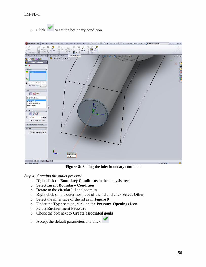
o Click to set the boundary condition
Figure 8: Setting the inlet boundary condition
Step 4: Creating the outlet pressure
o Right click on Boundary Conditions in the analysis tree
o Select Insert Boundary Condition
o Rotate to the circular lid and zoom in
o Right click on the outermost face of the lid and click Select Other
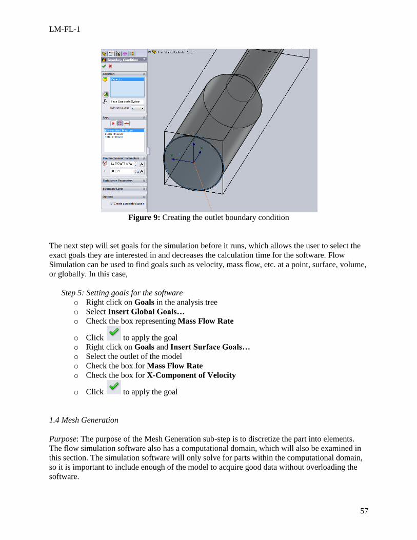
o Select the inner face of the lid as in Figure 9
o Under the Type section, click on the Pressure Openings icon
o Select Environment Pressure
o Check the box next to Create associated goals
o Accept the default parameters and click
LM-FL-1
57
Figure 9: Creating the outlet boundary condition
The next step will set goals for the simulation before it runs, which allows the user to select the
exact goals they are interested in and decreases the calculation time for the software. Flow
Simulation can be used to find goals such as velocity, mass flow, etc. at a point, surface, volume,
or globally. In this case,
Step 5: Setting goals for the software
o Right click on Goals in the analysis tree
o Select Insert Global Goals…
o Check the box representing Mass Flow Rate
o Click to apply the goal
o Right click on Goals and Insert Surface Goals…
o Select the outlet of the model
o Check the box for Mass Flow Rate
o Check the box for X-Component of Velocity
o Click to apply the goal
1.4 Mesh Generation
Purpose: The purpose of the Mesh Generation sub-step is to discretize the part into elements.
The flow simulation software also has a computational domain, which will also be examined in
this section. The simulation software will only solve for parts within the computational domain,
so it is important to include enough of the model to acquire good data without overloading the
software.
LM-FL-1
58
The only step in this section will be to adjust the mesh to a slightly finer setting to illustrate how
to acquire more accurate results.
Step 9: Adjusting the mesh
o Click on the Initial Mesh icon
o Adjust the Level of initial mesh dial to “6”
o Click OK to accept the changes
Figure 10: Adjusting the mesh settings
2. Solution
Purpose: The Solution is the step where the computer solves the simulation problem and
generates results for use in the Post-Processing step.
Step 1: Running the simulation
o At the top of the screen, click
LM-FL-1
59
o Make sure New calculation is selected and the Take previous results box is not
checked as in Figure 11
o Click Run
o The solver window will pop-up and notify when the simulation is finished
Figure 11: Running a study from scratch
3. Post-Processing
Purpose: The purpose of the Post-Processing step is to process the results of interest. For this
problem, various plot tools will be utilized and the goals will be exported to a spreadsheet.
SolidWorks Flow Simulation has multiple ways of creating charts and graphs. For example,
Figure 12 shows three different ways to insert flow trajectories into the model. All three of these
will create the same graph so feel free to use whichever is most convenient, however this module
will work from the analysis tree for consistency.
LM-FL-1
60
Figure 12: Various ways to select the same feature
The first plot in the post-processing step is setting up flow trajectories. Flow trajectories trace the
flow of the fluid from a set starting point to the edge of the computational domain. The plot will
show output such as velocity or pressure at specified intervals along the fluid path. With
SolidWorks Flow Simulation, the number of trajectories can be defined along with the display
type. In this case, 20 spherical flow trajectories will be inserted at the inlet of the volume and
they will trace the air flow through the room and out the circular duct.
Step1: Inserting flow trajectories
o Right click on Flow Trajectories from the analysis tree
o Select Insert
o Underneath Starting Points, choose the Reference icon and click on the inner face of the
lid as in Figure XX
o Type “20” into Number of flow trajectories
o Use the dropdown menu next to Draw trajectories as to select Spheres
o Type “3 in” in the Cross Size box
o Click on View Settings… and navigate to the Contours tab
o Change Parameter to Velocity to directly set the plot to display velocity
o Click OK
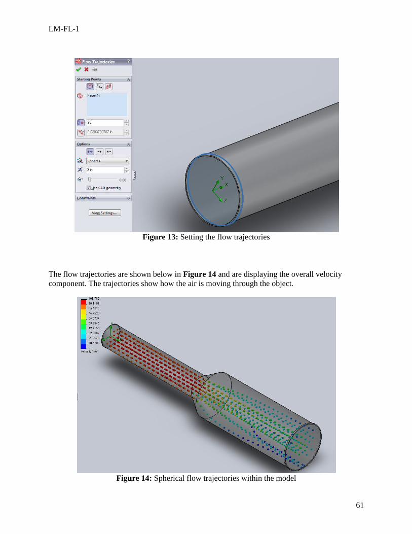
o Verify settings with Figure 13 and click
Drop down menu
Directly select
Right click from analysis
tree
LM-FL-1
61
Figure 13: Setting the flow trajectories
The flow trajectories are shown below in Figure 14 and are displaying the overall velocity
component. The trajectories show how the air is moving through the object.
Figure 14: Spherical flow trajectories within the model
LM-FL-1
62
The plot above shows a final view of the 20 flow trajectories inserted into the model. The
spheres give a different look to the flow trajectories than the arrows or pipes, but the data is the
same. Animating the plot can illustrate how the particles move through the model slightly better.
Step 2: Animating the plot
o Right click on the flow trajectories plot, Flow Trajectories 1
o Select Animate…
o Use the play button at the bottom of the screen to start the animation
o The settings can be adjusted by clicking the More… icon
o Click to save the animation or to exit without saving
The next plot to examine is a cut plot, which will be used to show the velocity all along the
model. This plot can also be animated and can be very useful if animated from different
directions such as from the front, right, and top planes.
Step 3: Creating a cut plot
o Hide the flow trajectories plot by right clicking on it and selecting Hide
o Right click on Cut Plots in the analysis tree
o Select Insert
o Use the Reference icon in the Selection box
o Select the Front Plane from the design tree
o Verify with Figure 15 and click to create the plot
LM-FL-1
63
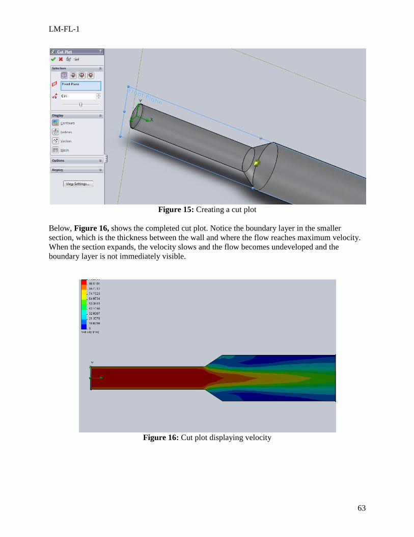
Figure 15: Creating a cut plot
Below, Figure 16, shows the completed cut plot. Notice the boundary layer in the smaller
section, which is the thickness between the wall and where the flow reaches maximum velocity.
When the section expands, the velocity slows and the flow becomes undeveloped and the
boundary layer is not immediately visible.
Figure 16: Cut plot displaying velocity
LM-FL-1
64
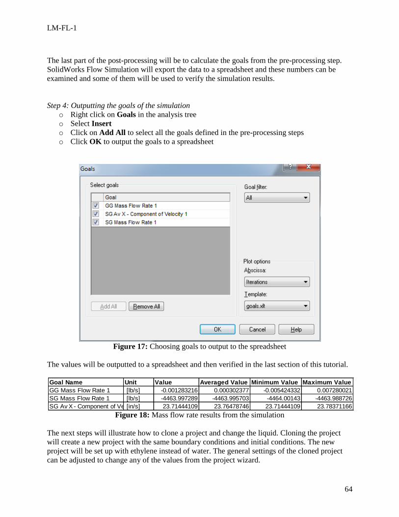
The last part of the post-processing will be to calculate the goals from the pre-processing step.
SolidWorks Flow Simulation will export the data to a spreadsheet and these numbers can be
examined and some of them will be used to verify the simulation results.
Step 4: Outputting the goals of the simulation
o Right click on Goals in the analysis tree
o Select Insert
o Click on Add All to select all the goals defined in the pre-processing steps
o Click OK to output the goals to a spreadsheet
Figure 17: Choosing goals to output to the spreadsheet
The values will be outputted to a spreadsheet and then verified in the last section of this tutorial.
Figure 18: Mass flow rate results from the simulation
The next steps will illustrate how to clone a project and change the liquid. Cloning the project
will create a new project with the same boundary conditions and initial conditions. The new
project will be set up with ethylene instead of water. The general settings of the cloned project
can be adjusted to change any of the values from the project wizard.
Goal Name Unit Value Averaged Value Minimum Value Maximum Value
GG Mass Flow Rate 1 [lb/s] -0.001283216 0.000302377 -0.005424332 0.007280021
SG Mass Flow Rate 1 [lb/s] -4463.997289 -4463.995703 -4464.00143 -4463.988726
SG Av X - Component of Velocity 1 [in/s] 23.71444109 23.76478746 23.71444109 23.78371166

LM-FL-1
65
Step 5: Cloning the project
o Expand Flow Simulation, choose Project, and select Clone Project
o Select the Create new option
o Change configuration name to “Expanding flow with Ethylene”
Step 6: Changing the general settings for a project
o Click to open up the general settings menu
o Click on Fluids in the Navigator section
o Highlight “Water (Liquids)” in the Project Fluids section and click Remove
o Expand the Liquids section and highlight “Ethylene”
o Click Add and verify the settings with Figure 17
o Click OK to accept the settings
Figure 17: Changing the general settings
The boundary conditions and mesh should already be defined from the previous study. Click on
Run to gather the new results. After the simulation is done running, double click on either of the
plots created earlier to re-display them with the new fluid.
The next plot to look at is an XY Plot, which outputs data to a spreadsheet. In this case, the
velocity will be plotted along the vertical lines that intersect the midpoint of the small and large
sections of the model.
Step 7: Creating an XY Plot
o Right click on XY Plots in the analysis tree
LM-FL-1
66
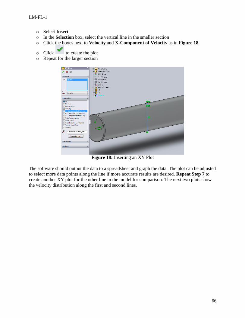
o Select Insert
o In the Selection box, select the vertical line in the smaller section
o Click the boxes next to Velocity and X-Component of Velocity as in Figure 18
o Click to create the plot
o Repeat for the larger section
Figure 18: Inserting an XY Plot
The software should output the data to a spreadsheet and graph the data. The plot can be adjusted
to select more data points along the line if more accurate results are desired. Repeat Step 7 to
create another XY plot for the other line in the model for comparison. The next two plots show
the velocity distribution along the first and second lines.
LM-FL-1
67
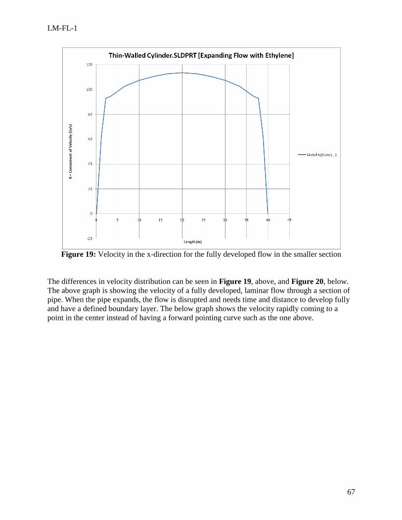
Figure 19: Velocity in the x-direction for the fully developed flow in the smaller section
The differences in velocity distribution can be seen in Figure 19, above, and Figure 20, below.
The above graph is showing the velocity of a fully developed, laminar flow through a section of
pipe. When the pipe expands, the flow is disrupted and needs time and distance to develop fully
and have a defined boundary layer. The below graph shows the velocity rapidly coming to a
point in the center instead of having a forward pointing curve such as the one above.
LM-FL-1
68
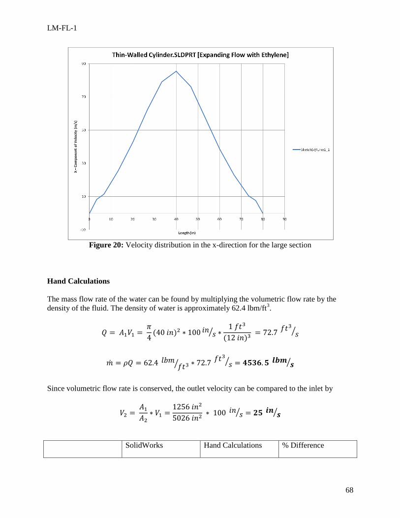
Figure 20: Velocity distribution in the x-direction for the large section
Hand Calculations
The mass flow rate of the water can be found by multiplying the volumetric flow rate by the
density of the fluid. The density of water is approximately 62.4 lbm/ft3.
⁄
⁄
⁄
⁄ ⁄
Since volumetric flow rate is conserved, the outlet velocity can be compared to the inlet by
⁄ ⁄
SolidWorks Hand Calculations % Difference
LM-FL-1
69
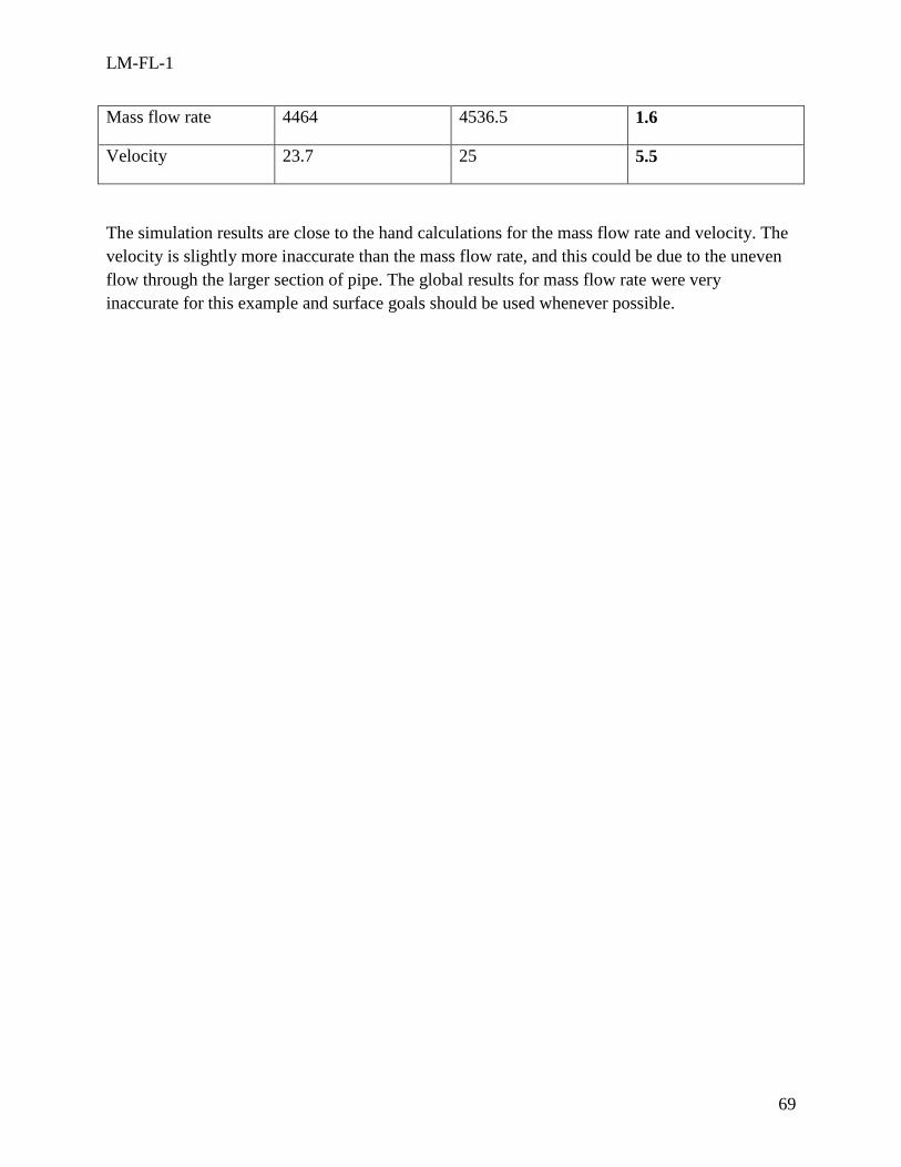
Mass flow rate 4464 4536.5 1.6
Velocity 23.7 25 5.5
The simulation results are close to the hand calculations for the mass flow rate and velocity. The
velocity is slightly more inaccurate than the mass flow rate, and this could be due to the uneven
flow through the larger section of pipe. The global results for mass flow rate were very
inaccurate for this example and surface goals should be used whenever possible.

LM-FL-1
70
Attachment D. CoMetSolution-Specific FEM Tutorials
LM-FL-1
71
Attachment E. Post-Test
1. Which of the following is true about setting goals in Flow Simulation?
o Goals must be defined before the simulation has run to acquire results
o Goals allow the user to acquire specific data from the simulation
o The user can set global goals as well as goals for a surface or point
o All the above
2. If an internal flow analysis has an inlet velocity, what other boundary condition must be
applied for a proper simulation to run?
o Outlet velocity
o Pressure
o Inlet volumetric flow rate
o Outlet mass flow rate
3. Which of the following situations would not be suitable for internal analysis?
o Airflow through a duct system
o Water running though a pipe
o Ethylene passing through a heat exchanger
o Airflow past an airfoil
4. The area in which the flow simulation carries out the calculations is called the
o Computational domain
o Mesh
o Flow space
o Calculation control
5. Which of the following are user-specified initial conditions in an external flow analysis?
o Velocity
o Pressure
o Temperature
o All the above
6. Which of the following is not a boundary condition in flow simulation?
o Environmental pressure
o Mass flow rate
o Static pressure

LM-FL-1
72
o Fluid viscosity
7. What parameter would be adjusted to discretize the model into smaller parts for
computation?
o Computational domain
o Mesh
o Fluid sub-domain
o Initial goals
8. Where can boundary conditions be placed in the model?
o Between a solid and fluid boundary
o At the outer face of a lid
o Along an outer edge
o Outside of the computational domain
9. Which plot is ideal for looking at how the fluid flows through the model?
o Cut plot
o 3-D surface plot
o Flow trajectories plot
o XY plot
10. What tool is used to cover any openings in an internal fluid analysis and create a fully
enclosed volume?
o Computational domain
o Boundary conditions
o Lids
o Mesh
11. Explain how to create and animate a fluid trajectories plot
12. Explain how to create an XY plot from an edge or line

LM-FL-1
73
Attachment F. Practice Problems
Problem 1:
Water passes through a rectangular box at 15 m/s and the flow is fully developed. Calculate the
volumetric flow rate and plot the velocity along the y direction.
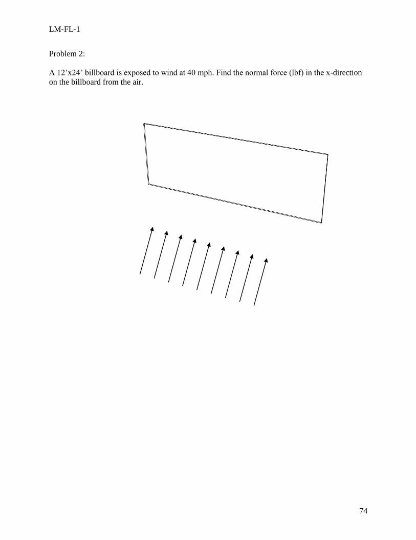
LM-FL-1
74
Problem 2:
A 12’x24’ billboard is exposed to wind at 40 mph. Find the normal force (lbf) in the x-direction
on the billboard from the air.

LM-FL-1
75
Problem 3:
A truck is driving down the highway at 70 mph. Calculate the average drag force on each of the
two surfaces shown below and plot two flow trajectories: one with velocity and one with
pressure.
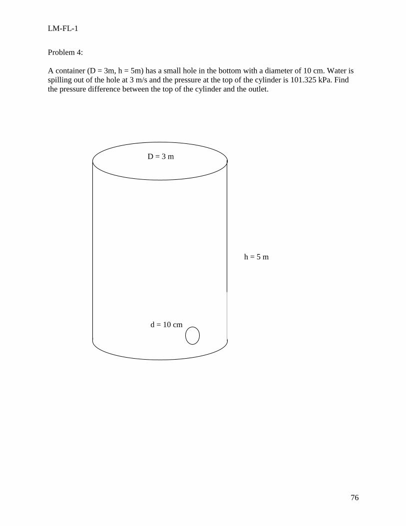
LM-FL-1
76
Problem 4:
A container (D = 3m, h = 5m) has a small hole in the bottom with a diameter of 10 cm. Water is
spilling out of the hole at 3 m/s and the pressure at the top of the cylinder is 101.325 kPa. Find
the pressure difference between the top of the cylinder and the outlet.
d = 10 cm
h = 5 m
D = 3 m
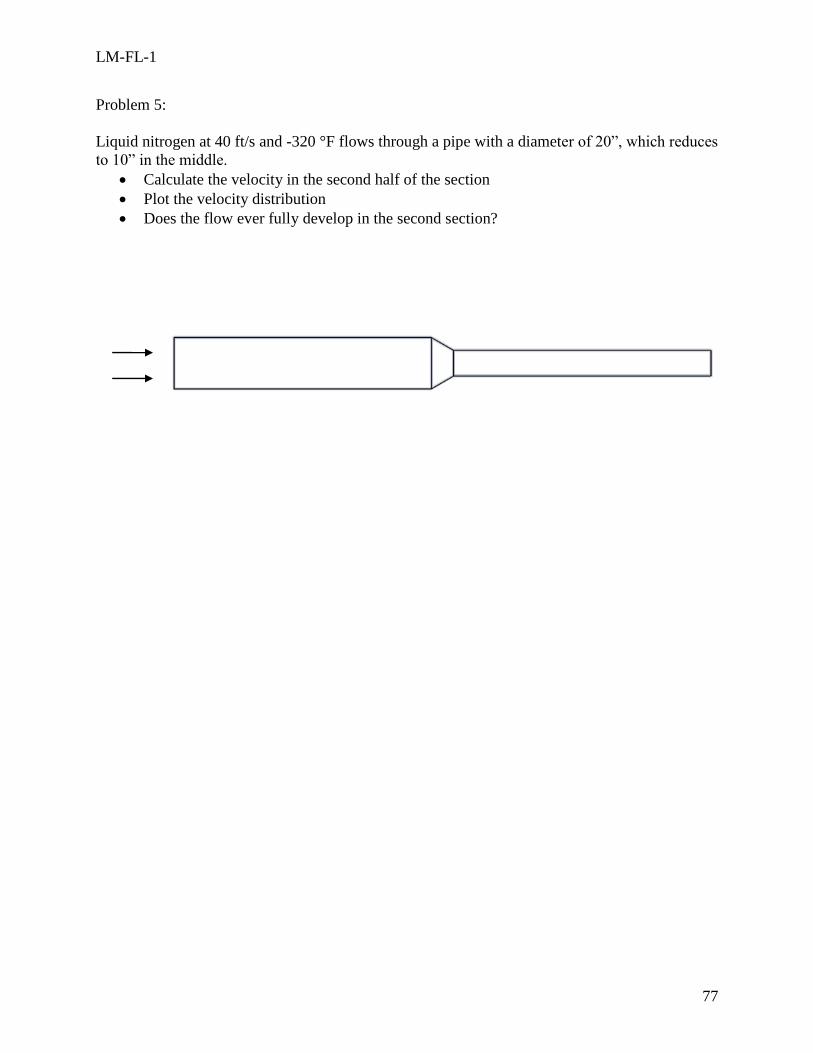
LM-FL-1
77
Problem 5:
Liquid nitrogen at 40 ft/s and -320 °F flows through a pipe with a diameter of 20”, which reduces
to 10” in the middle.
Calculate the velocity in the second half of the section
Plot the velocity distribution
Does the flow ever fully develop in the second section?
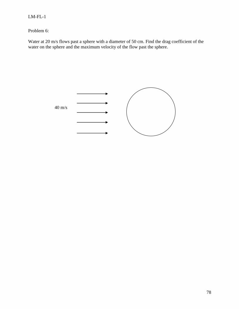
LM-FL-1
78
Problem 6:
Water at 20 m/s flows past a sphere with a diameter of 50 cm. Find the drag coefficient of the
water on the sphere and the maximum velocity of the flow past the sphere.
40 m/s
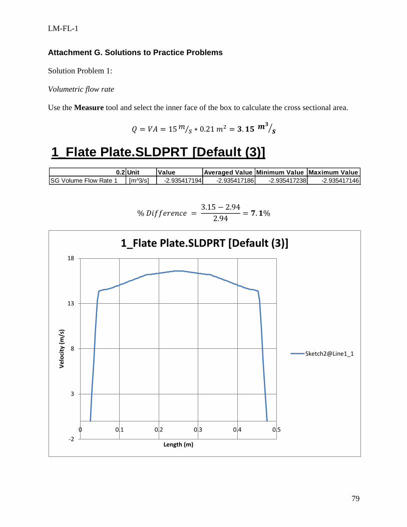
LM-FL-1
79
Attachment G. Solutions to Practice Problems
Solution Problem 1:
Volumetric flow rate
Use the Measure tool and select the inner face of the box to calculate the cross sectional area.
⁄
⁄
1_Flate Plate.SLDPRT [Default (3)]
0.2 Unit Value Averaged Value Minimum Value Maximum Value
SG Volume Flow Rate 1 [m 3/s] -2.935417194 -2.935417186 -2.935417238 -2.935417146
-2
3
8
13
18
0 0.1 0.2 0.3 0.4 0.5
Ve
loci
ty (
m/s
)
Length (m)
1_Flate Plate.SLDPRT [Default (3)]
Sketch2@Line1_1
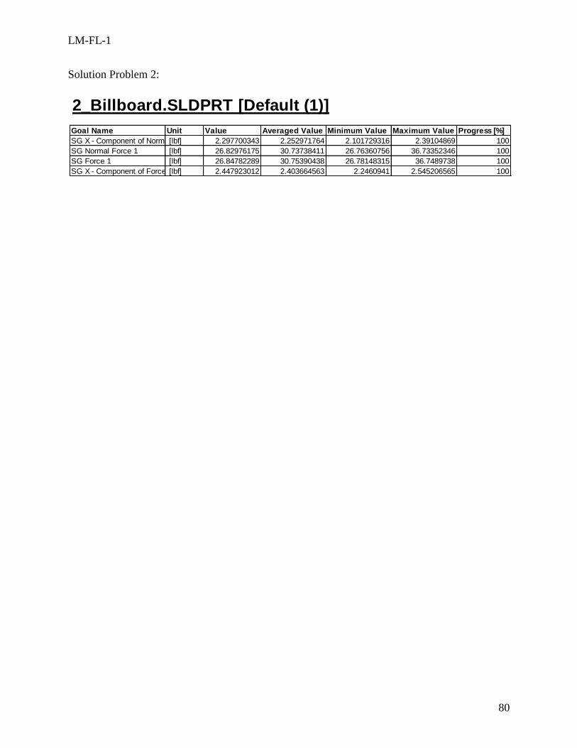
LM-FL-1
80
Solution Problem 2:
2_Billboard.SLDPRT [Default (1)]
Goal Name Unit Value Averaged Value Minimum Value Maximum Value Progress [%]
SG X - Component of Normal Force 1 [lbf] 2.297700343 2.252971764 2.101729316 2.39104869 100
SG Normal Force 1 [lbf] 26.82976175 30.73738411 26.76360756 36.73352346 100
SG Force 1 [lbf] 26.84782289 30.75390438 26.78148315 36.7489738 100
SG X - Component of Force 1 [lbf] 2.447923012 2.403664563 2.2460941 2.545206565 100
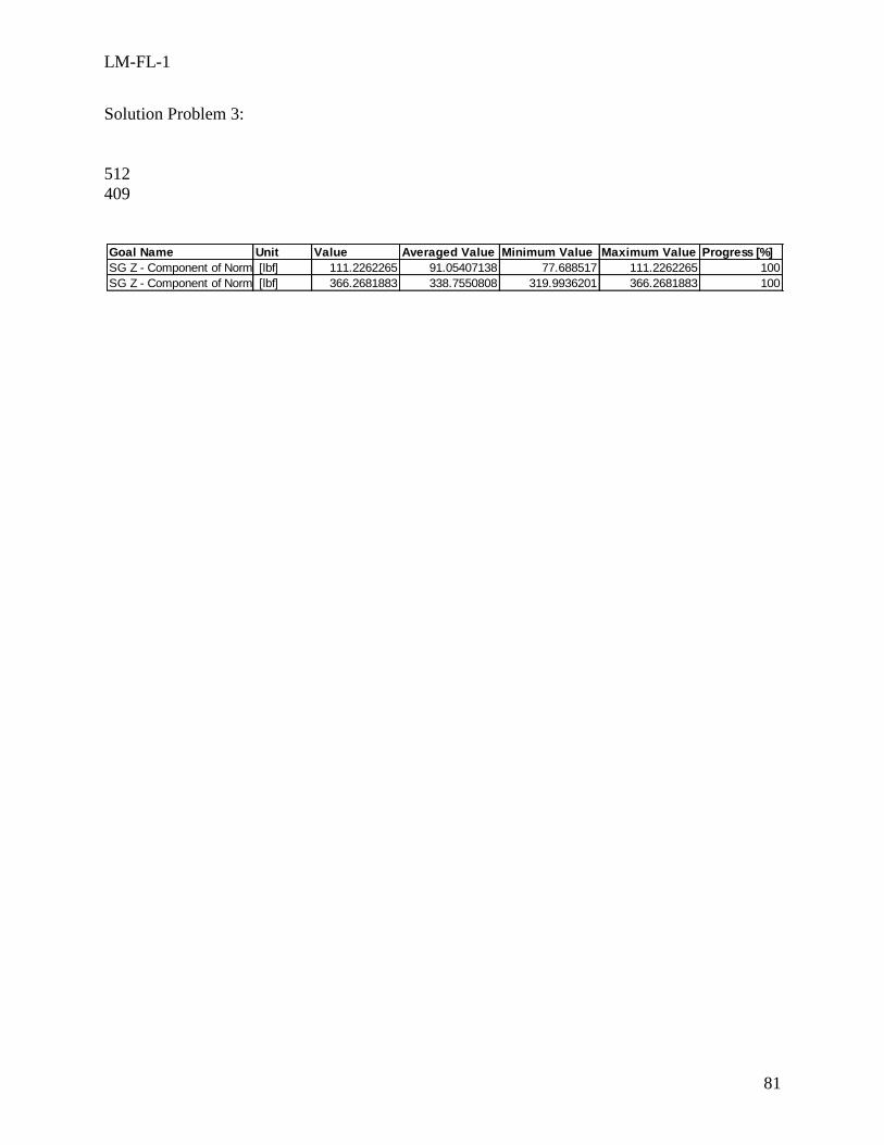
LM-FL-1
81
Solution Problem 3:
512
409
Goal Name Unit Value Averaged Value Minimum Value Maximum Value Progress [%]
SG Z - Component of Normal Force 1 [lbf] 111.2262265 91.05407138 77.688517 111.2262265 100
SG Z - Component of Normal Force 2 [lbf] 366.2681883 338.7550808 319.9936201 366.2681883 100
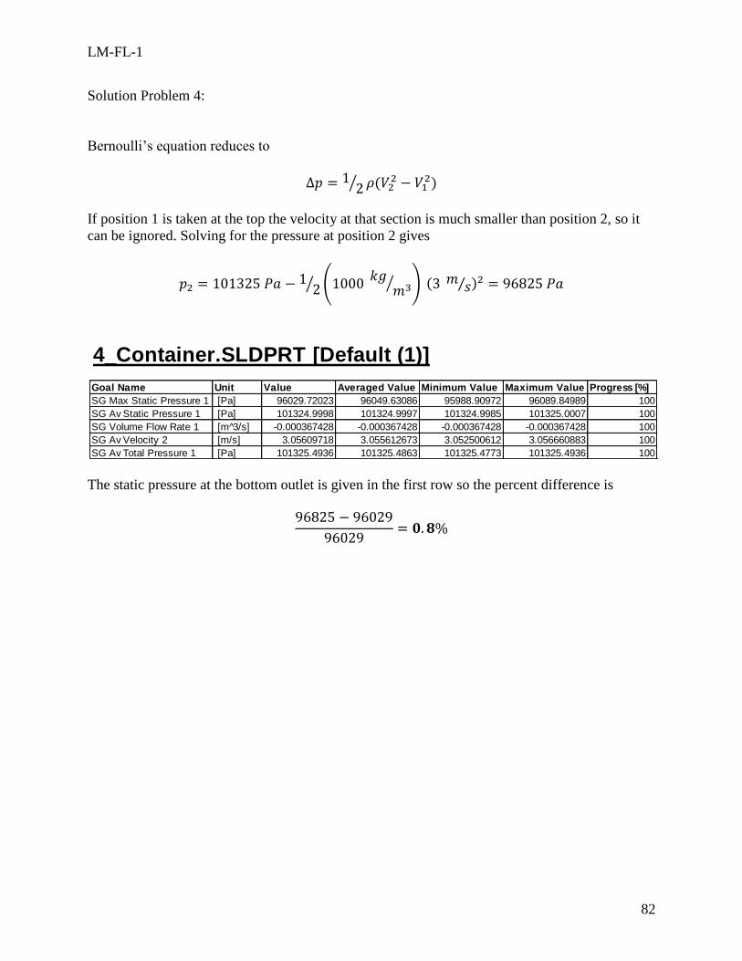
LM-FL-1
82
Solution Problem 4:
Bernoulli’s equation reduces to
⁄
If position 1 is taken at the top the velocity at that section is much smaller than position 2, so it
can be ignored. Solving for the pressure at position 2 gives
⁄ (
⁄ ) ⁄
The static pressure at the bottom outlet is given in the first row so the percent difference is
4_Container.SLDPRT [Default (1)]
Goal Name Unit Value Averaged Value Minimum Value Maximum Value Progress [%]
SG Max Static Pressure 1 [Pa] 96029.72023 96049.63086 95988.90972 96089.84989 100
SG Av Static Pressure 1 [Pa] 101324.9998 101324.9997 101324.9985 101325.0007 100
SG Volume Flow Rate 1 [m 3/s] -0.000367428 -0.000367428 -0.000367428 -0.000367428 100
SG Av Velocity 2 [m/s] 3.05609718 3.055612673 3.052500612 3.056660883 100
SG Av Total Pressure 1 [Pa] 101325.4936 101325.4863 101325.4773 101325.4936 100
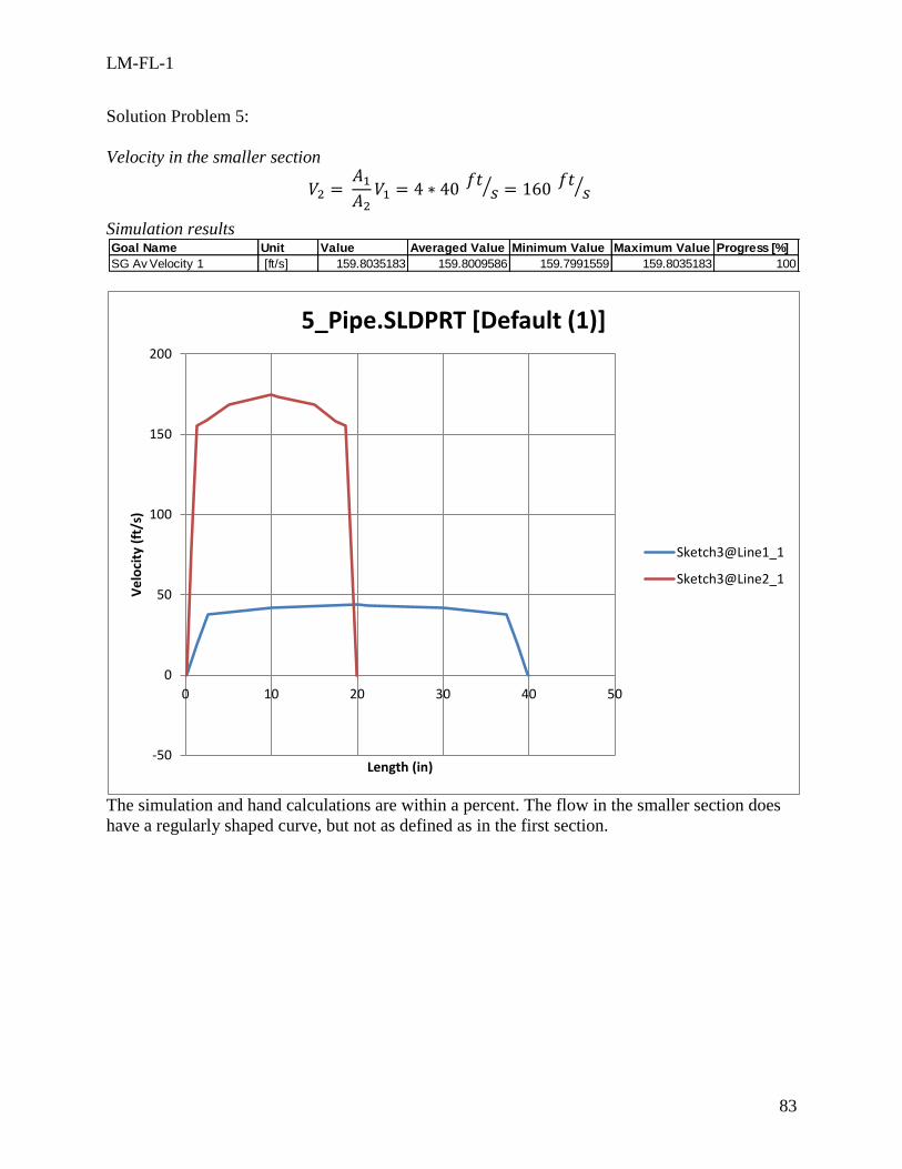
LM-FL-1
83
Solution Problem 5:
Velocity in the smaller section
⁄
⁄
Simulation results
The simulation and hand calculations are within a percent. The flow in the smaller section does
have a regularly shaped curve, but not as defined as in the first section.
Goal Name Unit Value Averaged Value Minimum Value Maximum Value Progress [%]
SG Av Velocity 1 [ft/s] 159.8035183 159.8009586 159.7991559 159.8035183 100
-50
0
50
100
150
200
0 10 20 30 40 50
Ve
loci
ty (
ft/s
)
Length (in)
5_Pipe.SLDPRT [Default (1)]
Sketch3@Line1_1
Sketch3@Line2_1
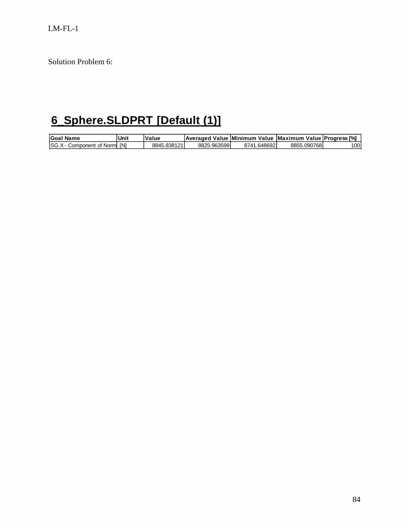
LM-FL-1
84
Solution Problem 6:
6_Sphere.SLDPRT [Default (1)]
Goal Name Unit Value Averaged Value Minimum Value Maximum Value Progress [%]
SG X - Component of Normal Force 1 [N] 8845.838121 8825.963599 8741.648692 8855.090768 100
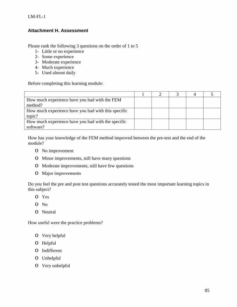
LM-FL-1
85
Attachment H. Assessment
Please rank the following 3 questions on the order of 1 to 5
1- Little or no experience
2- Some experience
3- Moderate experience
4- Much experience
5- Used almost daily
Before completing this learning module:
1 2 3 4 5
How much experience have you had with the FEM
method?
How much experience have you had with this specific
topic?
How much experience have you had with the specific
software?
How has your knowledge of the FEM method improved between the pre-test and the end of the
module?
o No improvement
o Minor improvements, still have many questions
o Moderate improvements, still have few questions
o Major improvements
Do you feel the pre and post test questions accurately tested the most important learning topics in
this subject?
o Yes
o No
o Neutral
How useful were the practice problems?
o Very helpful
o Helpful
o Indifferent
o Unhelpful
o Very unhelpful
LM-FL-1
86
Do you feel there was sufficient material contained in the learning module to answer all the post
test questions and complete the FEM analysis of the practice problems?
o Yes
o No
If yes, did you acquire help from an outside source or complete the module on your
own?
If not, which problems/concepts did you struggle with?
Do you feel it was bad to not have a teacher there to answer any questions you might have?
o It didn’t matter
o It would have been nice
o I really wanted to ask a question
How did the interactivity of the program affect your learning?
o Improved it a lot
o Improved it some
o No difference
o Hurt it some
o Hurt it a lot
The six levels of Bloom’s Taxonomy are listed below. Rank how well this learning module
covers each level, with 5 meaning exceptionally well and 1 meaning very poor.
1. Knowledge (remembering previously learned material)
O 5
O 4
O 3
O 2
O 1
2. Comprehension (the ability to grasp the meaning of the material and give examples)
LM-FL-1
87
O 5
O 4
O 3
O 2
O 1
3. Application (the ability to use the material in new situations)
O 5
O 4
O 3
O 2
O 1
4. Analysis (the ability to break down material into its component parts so that its
organizational structure may be understood)
O 5
O 4
O 3
O 2
O 1
5. Synthesis (the ability to put parts together to form a new whole)
O 5
O 4
O 3
O 2
O 1
6. Evaluation (the ability to judge the value of the material for a given purpose)
O 5
O 4
O 3
O 2
O 1
Do you think the mixed text and video format works well?
o Yes
o Indifferent
o No
Do you think the module presents an effective method of learning FEA?
LM-FL-1
88
o Yes
o Indifferent
o No
Did you prefer this module over the traditional classroom learning experience? Why or why not.
How accurate would it be to call this module self-contained and stand-alone?
o Very accurate
o Accurate
o Indifferent
o Inaccurate
o Very inaccurate
What specifically did you like and/or dislike about the module.
Was there any part of the module that you felt was unnecessary of redundant? Was there a need
for any additional parts?
Please list any suggestions for improving this module.

LM-FL-1
89
Overall, how would you rate your experience taking this module?
o Excellent
o Fair
o Average
o Poor
o Awful


![[Data Sheet] F Series Gen3 - s3.ap-northeast · PDF filelm/W 3500 154 171 190 4000 157 175 194 5000 162 181 201 CCT ... Dimension Specification Tolerance Unit Module Length 560.0 0.3](https://img.pdfslide.net/doc/110x75/5a72c8e17f8b9aa2538dfecf/data-sheet-f-series-gen3-s3ap-northeast-lmw-3500-154-171-190-4000.jpg)


![]M?>ADBC O^C K]EB@ TVJLD`EH[?C1=?C aLDBC C · PDF filelm* .n6o2:pq 4ec pr.s4t*u47-wvopo2yx -3](https://img.pdfslide.net/doc/110x75/5a9515f27f8b9a18628c8bbb/madbc-oc-keb-tvjldehc1c-aldbc-c-n6o2pq-4ec-prs4tu47-wvopo2yx-3on254zk.jpg)