Learning Particle Physics by Example: Location-Aware ... · Learning Particle Physics by Example: Location-Aware Generative Adversarial Networks for Physics Synthesis ... simulations

Learning Particle Physics by Example:

Location-Aware Generative Adversarial Networks for

Physics Synthesis

Luke de Oliveiraa, Michela Paganinia,b, and Benjamin Nachmana

aLawrence Berkeley National Laboratory, 1 Cyclotron Rd, Berkeley, CA, 94720, USAbDepartment of Physics, Yale University, New Haven, CT 06520, USA

E-mail: [email protected], [email protected], [email protected]

Abstract: We provide a bridge between generative modeling in the Machine Learning community

and simulated physical processes in High Energy Particle Physics by applying a novel Generative

Adversarial Network (GAN) architecture to the production of jet images – 2D representations of

energy depositions from particles interacting with a calorimeter. We propose a simple architecture,

the Location-Aware Generative Adversarial Network, that learns to produce realistic radiation patterns

from simulated high energy particle collisions. The pixel intensities of GAN-generated images faithfully

span over many orders of magnitude and exhibit the desired low-dimensional physical properties (i.e.,

jet mass, n-subjettiness, etc.). We shed light on limitations, and provide a novel empirical validation

of image quality and validity of GAN-produced simulations of the natural world. This work provides

a base for further explorations of GANs for use in faster simulation in High Energy Particle Physics.

arX

iv:1

701.

0592

7v2

[st

at.M

L]

13

Jun

2017

mailto:[email protected], [email protected], [email protected]

1 Introduction

The task of learning a generative model of a data distribution has long been a very difficult, yet

rewarding research direction in the statistics and machine learning communities. Often positioned as

a complement to discriminative models, generative models face a more difficult challenge than their

discriminative counterparts, i.e., reproducing rich, structured distributions such as natural language,

audio, and images. Deep learning-based generative models, with the promise of hierarchical, end-to-

end learned features, are seen as one of the most promising avenues towards building generative models

capable of handling the most rich and non-linear of data spaces. Generative Adversarial Networks [1],

a relatively new framework for learning a deep generative model, cast the task as a two player non-

cooperative game between a generator network, G, and a discriminator network, D. The generator tries

to produce samples that the discriminator cannot distinguish as fake when compared to real samples

drawn from the data distribution, while the discriminator tries to correctly identify if a sample it

is shown originates from the generator (fake) or if it was sampled from the data distribution (real).

When we relax G and D to be from the space of all functions, there exists a unique equilibrium where

G reproduces the true data distribution, and D is 1/2 everywhere [1]. Most recent work on GANs

has focused on the task of recovering data distributions from natural images; many recent advances in

image generation using GANs have shown great promise in producing photo-realistic natural images

at high resolution [1–10] while attempting to solve many known problems with stability [4, 7] and lack

of convergence guarantees [11].

With the growing complexity of theoretical models and power of computers, many scientific and

engineering projects increasingly rely on detailed simulations and generative modeling. This is partic-

ularly true for High Energy Particle Physics where precise Monte Carlo (MC) simulations are used to

model physical processes spanning distance scales from 10−25 meters all the way to the macroscopic

distances of detectors. For example, both the ATLAS [12] and CMS [13] collaborations model the

detailed interactions of particles with matter to accurately describe the detector response. These full

simulations are based on the Geant4 package [14] and are time1 and CPU intensive, a significant

challenge given that O(109) events/year must be simulated. In fact, simulating this expansive dy-

namical range with the required precision is very expensive. Various approximations can be used to

make faster simulations [15–17], but the time is still non-negligible and they are not applicable in all

physics applications. Another potential bottleneck is the modeling of quark and gluon interactions on

the smallest distance scales (matrix element calculations). Calculations with a large number of final

state objects (e.g. higher order in the perturbative series) are very time consuming and can compete

with the detector simulation for the total event generation time. Recent work focusing on algorithmic

improvements that leverage High Performance Computing capabilities have helped combat long gen-

eration times [18]. However, not all processes are massively parallelizable and time at supercomputers

is a scarce resource.

Our goal is to develop a new paradigm for fast event generation in high energy physics through

the use of GANs. We start by tackling a constrained version of the larger problem, where we use

the concept of a jet image [19] to show that the idealized 2D radiation pattern from high energy

quarks and gluons can be efficiently and effectively reproduced by a GAN. This work builds upon

recent developments in jet image classification with deep neural networks [20–24]. By showing that

generated jet images resemble the true simulated images in physically meaningful ways, we demonstrate

the aptitude of GANs for future applications.

1Full simulation can take up to O(min/event).

– 1 –

This paper is organized as follows. Sections 2 and 3 provide a brief introductions to the physics

of jet images and structure of Generative Adversarial Networks, respectively. New GAN architectures

developed specifically for jet images are described in Sec. 4. The results from our model are shown in

Sec. 5, with an extensive discussion of what the neural network is learning. The paper concludes with

Sec. 6.

2 Dataset

Jets are the observable result of quarks and gluons scattering at high energy. A collimated stream of

protons and other hadrons forms in the direction of the initiating quark or gluon. Clusters of such

particles are called jets. A jet image is a two-dimensional representation of the radiation pattern within

a jet: the distribution of the locations and energies of the jet’s constituent particles. Jet formation

is finished well before it can be detected, so it is sufficient to consider the radiation pattern in a two

dimensional surface spanned by orthogonal angles2 η and φ. The jet image consists of a regular grid

of pixels in η×φ. This is analogous to a calorimeter without longitudinal segmentation (e.g. the CMS

detector [25]). Adding layers, either through longitudinal segmentation or combining information from

multiple detectors, has recently been studied for classification [22] and generation [26], but is beyond

the scope of this paper.

Jet images are constructed and pre-processed using the setup described in Ref. [20] and briefly

summarized in this section. The finite granularity of a calorimeter is simulated with a regular 0.1×0.1

grid in η and φ. The energy of each calorimeter cell is given by the sum of the energies of all

particles incident on the cell. Cells with positive energy are assigned to jets using the anti-kt clustering

algorithm [27] with a radius parameter of R = 1.0 via the software package FastJet 3.2.1 [28]. To

mitigate the contribution from the underlying event, jets are are trimmed [29] by re-clustering the

constituents into R = 0.3 kt subjets and dropping those which have less than 5% of the transverse

momentum of the parent jet. Trimming also reduces the impact of pileup: multiple proton-proton

collisions occurring in the same event as the hard-scatter process. Jet images are formed by translating

the η and φ of all constituents of a given jet so that its highest pT subjet is centered at the origin.

A rectangular grid of η × φ ∈ [−1.25, 1.25]× [−1.25, 1.25] with 0.1× 0.1 pixels centered at the origin

forms the basis of the jet image. The intensity of each pixel is the pT corresponding to the energy

and pseudorapditiy of the constituent calorimeter cell, pT = Ecell/ cosh(ηcell). The radiation pattern

is symmetric about the origin of the jet image and so the images are rotated3. The subjet with the

second highest pT (or, in its absence, the direction of the first principle component) is placed at an

angle of −π/2 with respect to the η − φ axes. Finally, a parity transform about the vertical axis is

applied if the left side of the image has more energy than the right side.

Jet images vary significantly depending on the process that produced them. One high profile

classification task is the separation of jets originating from high energy W bosons (signal) from generic

quark and gluon jets (background). Both signal and background are simulated using Pythia 8.219 [30,

31] at√s = 14 TeV. In order to mostly factor the impact of the jet transverse momentum (pT), we

focus on a particular range: 250 GeV < pjetT < 300 GeV. A typical jet image from the simulated

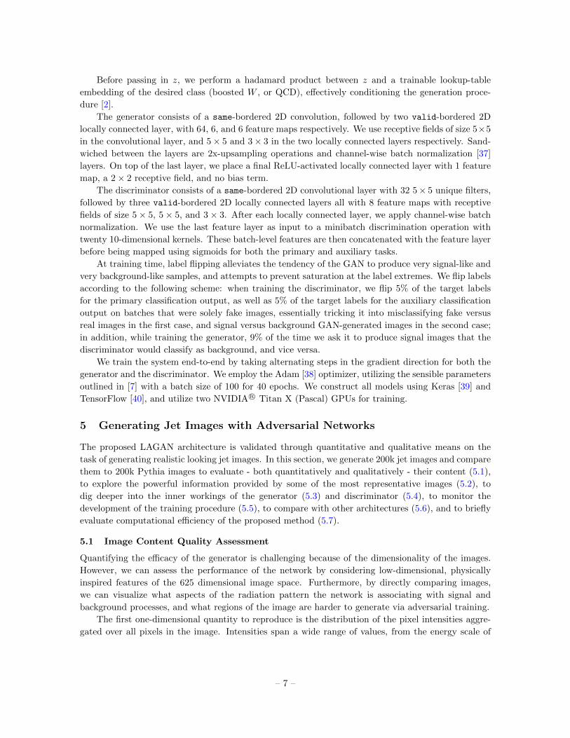
dataset [32] is shown in Fig. 1. The image has already been processed so that the leading subjet is

centered at the origin and the second highest pT subjet is at −π/2 in the translated η − φ space.

2While the azimuthal angle φ is a real angle, pseudorapidity η is only approximately equal to the polar angle θ.

However, the radiation pattern is nearly symmetric in φ and η and so these standard coordinates are used to describe

the jet constituent locations.3For more details about this rotation, which slightly differs from Ref. [20], see Appendix B.

– 2 –

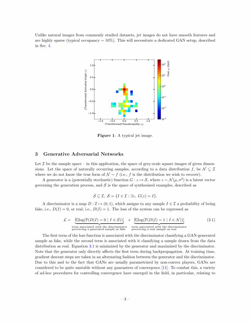
Unlike natural images from commonly studied datasets, jet images do not have smooth features and

are highly sparse (typical occupancy ∼ 10%). This will necessitate a dedicated GAN setup, described

in Sec. 4.

1.0 0.5 0.0 0.5 1.0[Transformed] Pseudorapidity (η)

1.0

0.5

0.0

0.5

1.0

[Tra

nsf

orm

ed]

Azi

muth

al A

ngle

(φ)

10-3

10-2

10-1

100

101

102

Pix

el pT (

GeV

)

Figure 1: A typical jet image.

3 Generative Adversarial Networks

Let I be the sample space – in this application, the space of grey-scale square images of given dimen-

sions. Let the space of naturally occurring samples, according to a data distribution f , be N ⊆ Iwhere we do not know the true form of N ∼ f (i.e., f is the distribution we wish to recover).

A generator is a (potentially stochastic) function G : z 7→ S, where z ∼ N (µ, σ2) is a latent vector

governing the generation process, and S is the space of synthesized examples, described as

S ⊆ I, S = {I ∈ I : ∃z, G(z) = I}.

A discriminator is a map D : I 7→ (0, 1), which assigns to any sample I ∈ I a probability of being

fake, i.e., D(I) = 0, or real, i.e., D(I) = 1. The loss of the system can be expressed as

L = E[log(P(D(I) = 0 | I ∈ S))]︸︷︷︸term associated with the discriminatorperceiving a generated sample as fake

+ E[log(P(D(I) = 1 | I ∈ N ))]︸︷︷︸term associated with the discriminatorperceiving a real sample as real

(3.1)

The first term of the loss function is associated with the discriminator classifying a GAN-generated

sample as fake, while the second term is associated with it classifying a sample drawn from the data

distribution as real. Equation 3.1 is minimized by the generator and maximized by the discriminator.

Note that the generator only directly affects the first term during backpropagation. At training time,

gradient descent steps are taken in an alternating fashion between the generator and the discriminator.

Due to this and to the fact that GANs are usually parametrized by non-convex players, GANs are

considered to be quite unstable without any guarantees of convergence [11]. To combat this, a variety

of ad-hoc procedures for controlling convergence have emerged in the field, in particular, relating to

– 3 –

the generation of natural images. Architectural constraints and optimizer configurations introduced

in [7] have provided a well studied set of defaults and starting points for training GANs.

Many newer improvements also help avoid mode collapse, a very common point of failure for

GANs where a generator learns to generate a single element of S that is maximally confusing for the

discriminator. For instance, mini-batch discrimination and feature matching [4] allow the discrimina-

tor to use batch-level features and statistics, effectively rendering mode collapse suboptimal for the

generator. It has also been empirically shown [2–4, 8] that adding auxiliary tasks seems to reduce

such a tendency and improve convergence stability; side information is therefore often used as either

additional information to the discriminator / generator [4, 5, 8], as a quantity to be reconstructed by

the discriminator [3, 6], or both [2].

4 Location-Aware Generative Adversarial Network(LAGANs)

We introduce a series of architectural modifications to the DCGAN [7] frameworks in order to take

advantage of the pixel-level symmetry properties of jet images while explicitly inducing location-based

feature detection.

We build an auxiliary task into our system following the ACGAN [2] formulation. In addition

to the primary task where the discriminator network must learn to identify fake jet images from real

ones, the discriminator is also tasked with jointly learning to classify boosted W bosons (signal) and

QCD (background), with the scope of learning the conditional data distribution.

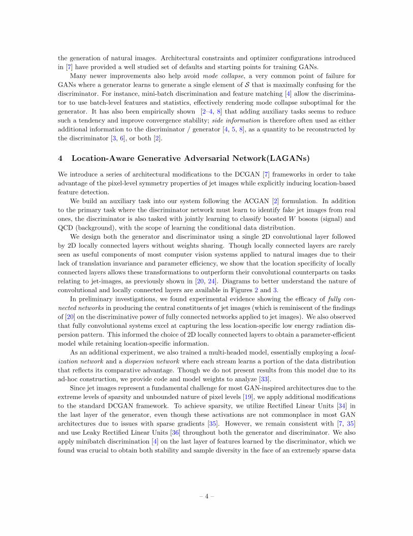
We design both the generator and discriminator using a single 2D convolutional layer followed

by 2D locally connected layers without weights sharing. Though locally connected layers are rarely

seen as useful components of most computer vision systems applied to natural images due to their

lack of translation invariance and parameter efficiency, we show that the location specificity of locally

connected layers allows these transformations to outperform their convolutional counterparts on tasks

relating to jet-images, as previously shown in [20, 24]. Diagrams to better understand the nature of

convolutional and locally connected layers are available in Figures 2 and 3.

In preliminary investigations, we found experimental evidence showing the efficacy of fully con-

nected networks in producing the central constituents of jet images (which is reminiscent of the findings

of [20] on the discriminative power of fully connected networks applied to jet images). We also observed

that fully convolutional systems excel at capturing the less location-specific low energy radiation dis-

persion pattern. This informed the choice of 2D locally connected layers to obtain a parameter-efficient

model while retaining location-specific information.

As an additional experiment, we also trained a multi-headed model, essentially employing a local-

ization network and a dispersion network where each stream learns a portion of the data distribution

that reflects its comparative advantage. Though we do not present results from this model due to its

ad-hoc construction, we provide code and model weights to analyze [33].

Since jet images represent a fundamental challenge for most GAN-inspired architectures due to the

extreme levels of sparsity and unbounded nature of pixel levels [19], we apply additional modifications

to the standard DCGAN framework. To achieve sparsity, we utilize Rectified Linear Units [34] in

the last layer of the generator, even though these activations are not commonplace in most GAN

architectures due to issues with sparse gradients [35]. However, we remain consistent with [7, 35]

and use Leaky Rectified Linear Units [36] throughout both the generator and discriminator. We also

apply minibatch discrimination [4] on the last layer of features learned by the discriminator, which we

found was crucial to obtain both stability and sample diversity in the face of an extremely sparse data

– 4 –

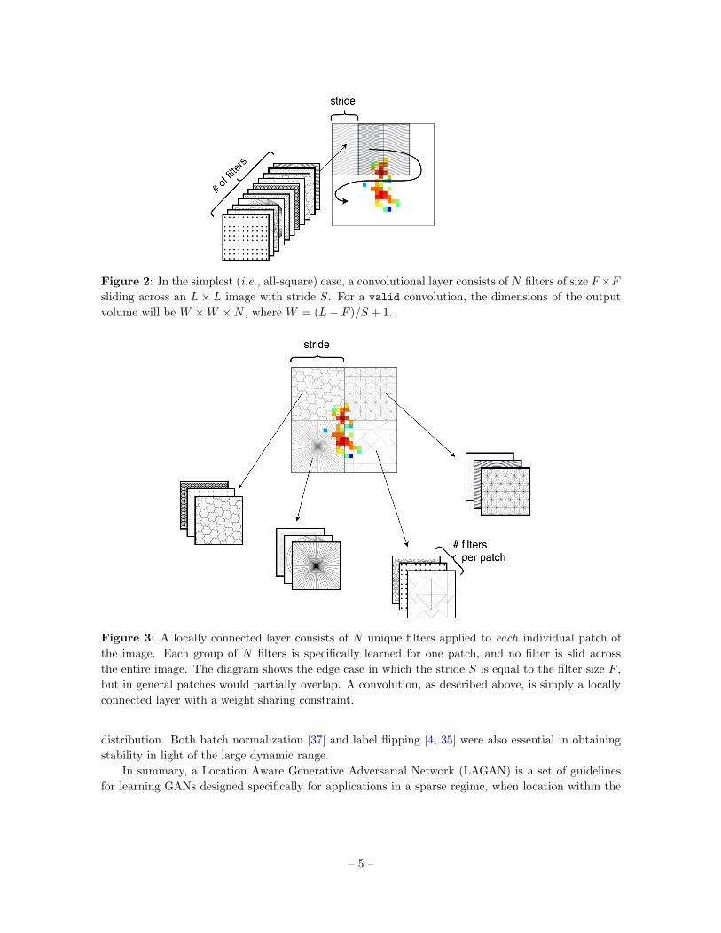
Figure 2: In the simplest (i.e., all-square) case, a convolutional layer consists of N filters of size F×Fsliding across an L × L image with stride S. For a valid convolution, the dimensions of the output

volume will be W ×W ×N , where W = (L− F )/S + 1.

Figure 3: A locally connected layer consists of N unique filters applied to each individual patch of

the image. Each group of N filters is specifically learned for one patch, and no filter is slid across

the entire image. The diagram shows the edge case in which the stride S is equal to the filter size F ,

but in general patches would partially overlap. A convolution, as described above, is simply a locally

connected layer with a weight sharing constraint.

distribution. Both batch normalization [37] and label flipping [4, 35] were also essential in obtaining

stability in light of the large dynamic range.

In summary, a Location Aware Generative Adversarial Network (LAGAN) is a set of guidelines

for learning GANs designed specifically for applications in a sparse regime, when location within the

– 5 –

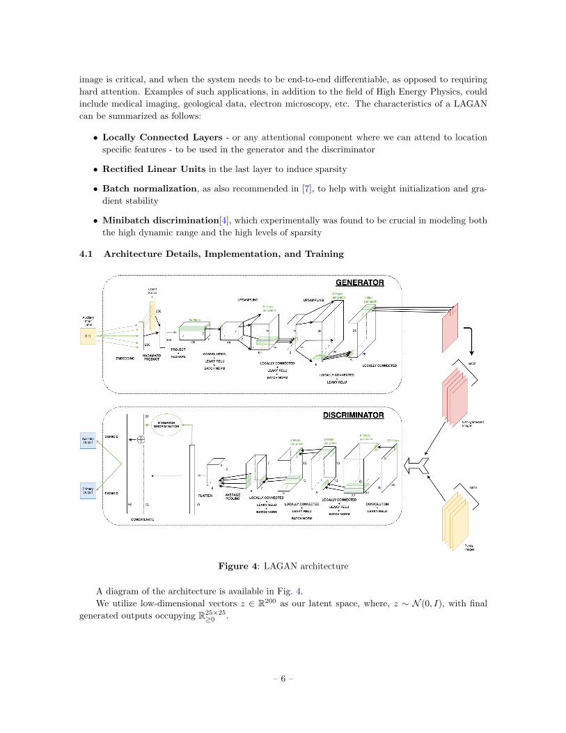
image is critical, and when the system needs to be end-to-end differentiable, as opposed to requiring

hard attention. Examples of such applications, in addition to the field of High Energy Physics, could

include medical imaging, geological data, electron microscopy, etc. The characteristics of a LAGAN

can be summarized as follows:

• Locally Connected Layers - or any attentional component where we can attend to location

specific features - to be used in the generator and the discriminator

• Rectified Linear Units in the last layer to induce sparsity

• Batch normalization, as also recommended in [7], to help with weight initialization and gra-

dient stability

• Minibatch discrimination[4], which experimentally was found to be crucial in modeling both

the high dynamic range and the high levels of sparsity

4.1 Architecture Details, Implementation, and Training

Figure 4: LAGAN architecture

A diagram of the architecture is available in Fig. 4.

We utilize low-dimensional vectors z ∈ R200 as our latent space, where, z ∼ N (0, I), with final

generated outputs occupying R25×25≥0 .

– 6 –

Before passing in z, we perform a hadamard product between z and a trainable lookup-table

embedding of the desired class (boosted W , or QCD), effectively conditioning the generation proce-

dure [2].

The generator consists of a same-bordered 2D convolution, followed by two valid-bordered 2D

locally connected layer, with 64, 6, and 6 feature maps respectively. We use receptive fields of size 5×5

in the convolutional layer, and 5× 5 and 3× 3 in the two locally connected layers respectively. Sand-

wiched between the layers are 2x-upsampling operations and channel-wise batch normalization [37]

layers. On top of the last layer, we place a final ReLU-activated locally connected layer with 1 feature

map, a 2× 2 receptive field, and no bias term.

The discriminator consists of a same-bordered 2D convolutional layer with 32 5× 5 unique filters,

followed by three valid-bordered 2D locally connected layers all with 8 feature maps with receptive

fields of size 5× 5, 5× 5, and 3× 3. After each locally connected layer, we apply channel-wise batch

normalization. We use the last feature layer as input to a minibatch discrimination operation with

twenty 10-dimensional kernels. These batch-level features are then concatenated with the feature layer

before being mapped using sigmoids for both the primary and auxiliary tasks.

At training time, label flipping alleviates the tendency of the GAN to produce very signal-like and

very background-like samples, and attempts to prevent saturation at the label extremes. We flip labels

according to the following scheme: when training the discriminator, we flip 5% of the target labels

for the primary classification output, as well as 5% of the target labels for the auxiliary classification

output on batches that were solely fake images, essentially tricking it into misclassifying fake versus

real images in the first case, and signal versus background GAN-generated images in the second case;

in addition, while training the generator, 9% of the time we ask it to produce signal images that the

discriminator would classify as background, and vice versa.

We train the system end-to-end by taking alternating steps in the gradient direction for both the

generator and the discriminator. We employ the Adam [38] optimizer, utilizing the sensible parameters

outlined in [7] with a batch size of 100 for 40 epochs. We construct all models using Keras [39] and

TensorFlow [40], and utilize two NVIDIA R© Titan X (Pascal) GPUs for training.

5 Generating Jet Images with Adversarial Networks

The proposed LAGAN architecture is validated through quantitative and qualitative means on the

task of generating realistic looking jet images. In this section, we generate 200k jet images and compare

them to 200k Pythia images to evaluate - both quantitatively and qualitatively - their content (5.1),

to explore the powerful information provided by some of the most representative images (5.2), to

dig deeper into the inner workings of the generator (5.3) and discriminator (5.4), to monitor the

development of the training procedure (5.5), to compare with other architectures (5.6), and to briefly

evaluate computational efficiency of the proposed method (5.7).

5.1 Image Content Quality Assessment

Quantifying the efficacy of the generator is challenging because of the dimensionality of the images.

However, we can assess the performance of the network by considering low-dimensional, physically

inspired features of the 625 dimensional image space. Furthermore, by directly comparing images,

we can visualize what aspects of the radiation pattern the network is associating with signal and

background processes, and what regions of the image are harder to generate via adversarial training.

The first one-dimensional quantity to reproduce is the distribution of the pixel intensities aggre-

gated over all pixels in the image. Intensities span a wide range of values, from the energy scale of

– 7 –

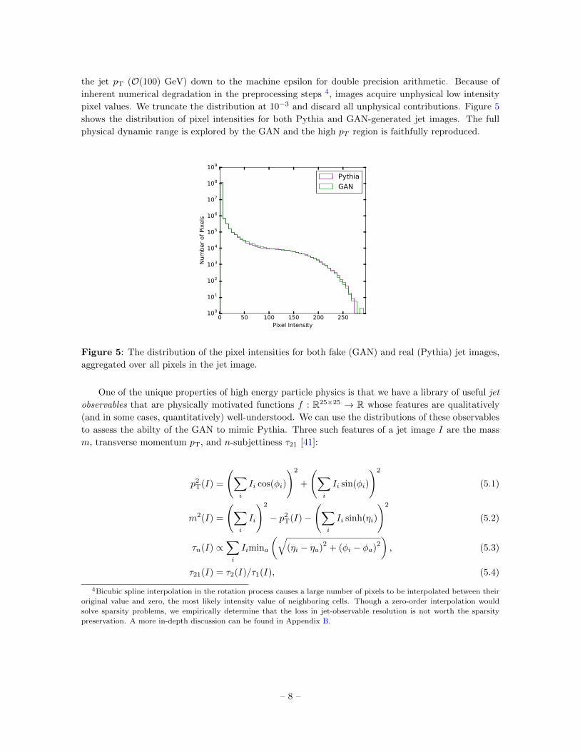
the jet pT (O(100) GeV) down to the machine epsilon for double precision arithmetic. Because of

inherent numerical degradation in the preprocessing steps 4, images acquire unphysical low intensity

pixel values. We truncate the distribution at 10−3 and discard all unphysical contributions. Figure 5

shows the distribution of pixel intensities for both Pythia and GAN-generated jet images. The full

physical dynamic range is explored by the GAN and the high pT region is faithfully reproduced.

0 50 100 150 200 250Pixel Intensity

100

101

102

103

104

105

106

107

108

109

Num

ber

of

Pix

els

Pythia

GAN

Figure 5: The distribution of the pixel intensities for both fake (GAN) and real (Pythia) jet images,

aggregated over all pixels in the jet image.

One of the unique properties of high energy particle physics is that we have a library of useful jet

observables that are physically motivated functions f : R25×25 → R whose features are qualitatively

(and in some cases, quantitatively) well-understood. We can use the distributions of these observables

to assess the abilty of the GAN to mimic Pythia. Three such features of a jet image I are the mass

m, transverse momentum pT, and n-subjettiness τ21 [41]:

p2T(I) =

(∑i

Ii cos(φi)

)2

+

(∑i

Ii sin(φi)

)2

(5.1)

m2(I) =

(∑i

Ii

)2

− p2T(I)−

(∑i

Ii sinh(ηi)

)2

(5.2)

τn(I) ∝∑i

Iimina

(√(ηi − ηa)

2+ (φi − φa)

2

), (5.3)

τ21(I) = τ2(I)/τ1(I), (5.4)

4Bicubic spline interpolation in the rotation process causes a large number of pixels to be interpolated between their

original value and zero, the most likely intensity value of neighboring cells. Though a zero-order interpolation would

solve sparsity problems, we empirically determine that the loss in jet-observable resolution is not worth the sparsity

preservation. A more in-depth discussion can be found in Appendix B.

– 8 –

where Ii, ηi, and φi are the pixel intensity, pseudorapidity, and azimuthal angle, respectively. The

sums run over the entire image. The quantities ηa and φa are axis values determined with the one-pass

kt axis selection using the winner-take-all combination scheme [42].

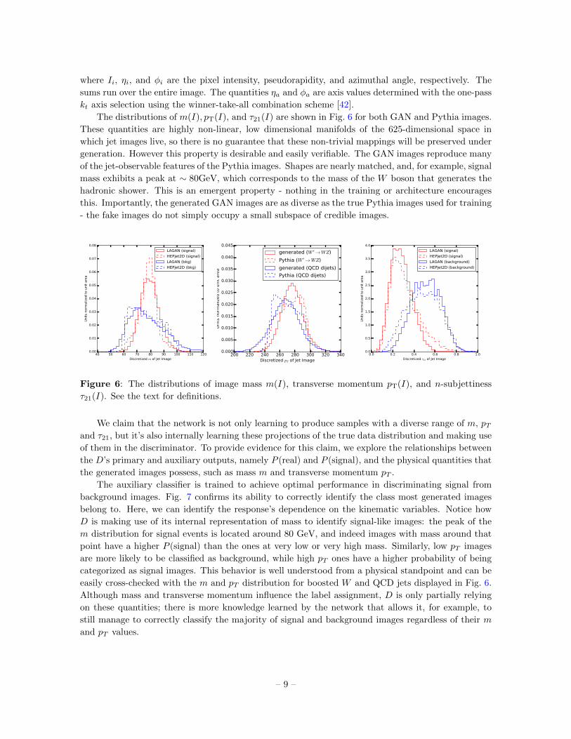
The distributions of m(I), pT(I), and τ21(I) are shown in Fig. 6 for both GAN and Pythia images.

These quantities are highly non-linear, low dimensional manifolds of the 625-dimensional space in

which jet images live, so there is no guarantee that these non-trivial mappings will be preserved under

generation. However this property is desirable and easily verifiable. The GAN images reproduce many

of the jet-observable features of the Pythia images. Shapes are nearly matched, and, for example, signal

mass exhibits a peak at ∼ 80GeV, which corresponds to the mass of the W boson that generates the

hadronic shower. This is an emergent property - nothing in the training or architecture encourages

this. Importantly, the generated GAN images are as diverse as the true Pythia images used for training

- the fake images do not simply occupy a small subspace of credible images.

40 50 60 70 80 90 100 110 120

Discretized m of Jet Image

0.00

0.01

0.02

0.03

0.04

0.05

0.06

0.07

0.08

Unit

s norm

aliz

ed t

o u

nit

are

a

LAGAN (signal)

HEPjet2D (signal)

LAGAN (bkg)

HEPjet2D (bkg)

200 220 240 260 280 300 320 340Discretized pT of Jet Image

0.000

0.005

0.010

0.015

0.020

0.025

0.030

0.035

0.040

0.045

Unit

s norm

aliz

ed t

o u

nit

are

a

generated (W ′→WZ)

Pythia (W ′→WZ)

generated (QCD dijets)

Pythia (QCD dijets)

0.0 0.2 0.4 0.6 0.8 1.0

Discretized τ21 of Jet Image

0.0

0.5

1.0

1.5

2.0

2.5

3.0

3.5

4.0

Unit

s norm

aliz

ed t

o u

nit

are

a

LAGAN (signal)

HEPjet2D (signal)

LAGAN (background)

HEPjet2D (background)

Figure 6: The distributions of image mass m(I), transverse momentum pT(I), and n-subjettiness

τ21(I). See the text for definitions.

We claim that the network is not only learning to produce samples with a diverse range of m, pTand τ21, but it’s also internally learning these projections of the true data distribution and making use

of them in the discriminator. To provide evidence for this claim, we explore the relationships between

the D’s primary and auxiliary outputs, namely P (real) and P (signal), and the physical quantities that

the generated images possess, such as mass m and transverse momentum pT .

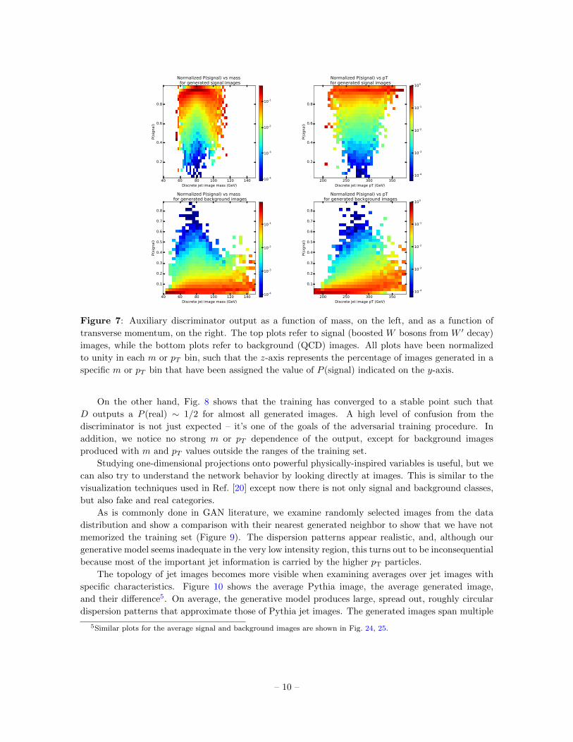
The auxiliary classifier is trained to achieve optimal performance in discriminating signal from

background images. Fig. 7 confirms its ability to correctly identify the class most generated images

belong to. Here, we can identify the response’s dependence on the kinematic variables. Notice how

D is making use of its internal representation of mass to identify signal-like images: the peak of the

m distribution for signal events is located around 80 GeV, and indeed images with mass around that

point have a higher P (signal) than the ones at very low or very high mass. Similarly, low pT images

are more likely to be classified as background, while high pT ones have a higher probability of being

categorized as signal images. This behavior is well understood from a physical standpoint and can be

easily cross-checked with the m and pT distribution for boosted W and QCD jets displayed in Fig. 6.

Although mass and transverse momentum influence the label assignment, D is only partially relying

on these quantities; there is more knowledge learned by the network that allows it, for example, to

still manage to correctly classify the majority of signal and background images regardless of their m

and pT values.

– 9 –

40 60 80 100 120 140Discrete jet image mass (GeV)

0.2

0.4

0.6

0.8

P(s

ignal)

Normalized P(signal) vs mass for generated signal images

10-4

10-3

10-2

10-1

200 250 300 350Discrete jet image pT (GeV)

0.2

0.4

0.6

0.8

P(s

ignal)

Normalized P(signal) vs pT for generated signal images

10-4

10-3

10-2

10-1

100


0.1

0.2

0.3

0.4

0.5

0.6

0.7

0.8

P(s

ignal)

Normalized P(signal) vs mass for generated background images

10-4

10-3

10-2

10-1


0.1

0.2

0.3

0.4

0.5

0.6

0.7

0.8

P(s

ignal)

Normalized P(signal) vs pT for generated background images

10-4

10-3

10-2

10-1

100

Figure 7: Auxiliary discriminator output as a function of mass, on the left, and as a function of

transverse momentum, on the right. The top plots refer to signal (boosted W bosons from W ′ decay)

images, while the bottom plots refer to background (QCD) images. All plots have been normalized

to unity in each m or pT bin, such that the z-axis represents the percentage of images generated in a

specific m or pT bin that have been assigned the value of P (signal) indicated on the y-axis.

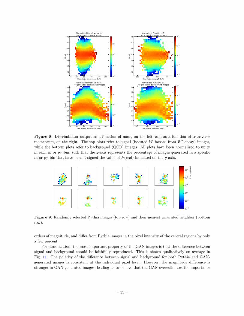
On the other hand, Fig. 8 shows that the training has converged to a stable point such that

D outputs a P (real) ∼ 1/2 for almost all generated images. A high level of confusion from the

discriminator is not just expected – it’s one of the goals of the adversarial training procedure. In

addition, we notice no strong m or pT dependence of the output, except for background images

produced with m and pT values outside the ranges of the training set.

Studying one-dimensional projections onto powerful physically-inspired variables is useful, but we

can also try to understand the network behavior by looking directly at images. This is similar to the

visualization techniques used in Ref. [20] except now there is not only signal and background classes,

but also fake and real categories.

As is commonly done in GAN literature, we examine randomly selected images from the data

distribution and show a comparison with their nearest generated neighbor to show that we have not

memorized the training set (Figure 9). The dispersion patterns appear realistic, and, although our

generative model seems inadequate in the very low intensity region, this turns out to be inconsequential

because most of the important jet information is carried by the higher pT particles.

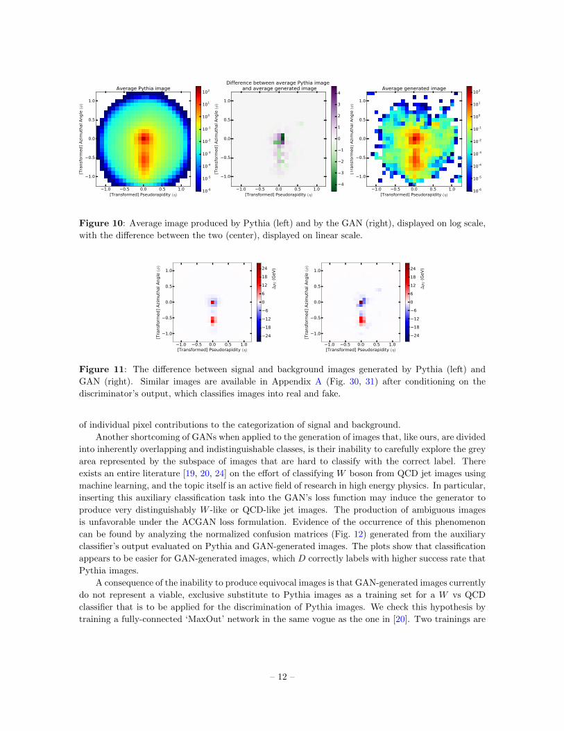
The topology of jet images becomes more visible when examining averages over jet images with

specific characteristics. Figure 10 shows the average Pythia image, the average generated image,

and their difference5. On average, the generative model produces large, spread out, roughly circular

dispersion patterns that approximate those of Pythia jet images. The generated images span multiple

5Similar plots for the average signal and background images are shown in Fig. 24, 25.

– 10 –


0.2

0.3

0.4

0.5

0.6

0.7

0.8

P(r

eal)

Normalized P(real) vs mass for generated signal images

10-4

10-3

10-2

10-1


0.2

0.3

0.4

0.5

0.6

0.7

0.8

P(r

eal)

Normalized P(real) vs pT for generated signal images

10-4

10-3

10-2

10-1

100


0.2

0.3

0.4

0.5

0.6

0.7

0.8

0.9

P(r

eal)

Normalized P(real) vs mass for generated background images

10-4

10-3

10-2

10-1


0.2

0.3

0.4

0.5

0.6

0.7

0.8

0.9

P(r

eal)

Normalized P(real) vs pT for generated background images

10-4

10-3

10-2

10-1

100

Figure 8: Discriminator output as a function of mass, on the left, and as a function of transverse

momentum, on the right. The top plots refer to signal (boosted W bosons from W ′ decay) images,

while the bottom plots refer to background (QCD) images. All plots have been normalized to unity

in each m or pT bin, such that the z-axis represents the percentage of images generated in a specific

m or pT bin that have been assigned the value of P (real) indicated on the y-axis.

10-3

10-2

10-1

100

101

102

Pix

el pT (

GeV

)

Figure 9: Randomly selected Pythia images (top row) and their nearest generated neighbor (bottom

row).

orders of magnitude, and differ from Pythia images in the pixel intensity of the central regions by only

a few percent.

For classification, the most important property of the GAN images is that the difference between

signal and background should be faithfully reproduced. This is shown qualitatively on average in

Fig. 11. The polarity of the difference between signal and background for both Pythia and GAN-

generated images is consistent at the individual pixel level. However, the magnitude difference is

stronger in GAN-generated images, leading us to believe that the GAN overestimates the importance

– 11 –


1.0

0.5

0.0

0.5

1.0

[Tra

nsf

orm

ed]

Azi

muth

al A

ngle

(φ)

Average Pythia image

10-6

10-5

10-4

10-3

10-2

10-1

100

101

102


1.0

0.5

0.0

0.5

1.0

[Tra

nsf

orm

ed]

Azi

muth

al A

ngle

(φ)

Difference between average Pythia image and average generated image

4

3

2

1

0

1

2

3

4


1.0

0.5

0.0

0.5

1.0

[Tra

nsf

orm

ed]

Azi

muth

al A

ngle

(φ)

Average generated image

10-6

10-5

10-4

10-3

10-2

10-1

100

101

102

Figure 10: Average image produced by Pythia (left) and by the GAN (right), displayed on log scale,

with the difference between the two (center), displayed on linear scale.


1.0

0.5

0.0

0.5

1.0

[Tra

nsf

orm

ed]

Azi

muth

al A

ngle

(φ)

24

18

12

6

0

6

12

18

24∆pT (

GeV

)


1.0

0.5

0.0

0.5

1.0

[Tra

nsf

orm

ed]

Azi

muth

al A

ngle

(φ)

24

18

12

6

0

6

12

18

24

∆pT (

GeV

)

Figure 11: The difference between signal and background images generated by Pythia (left) and

GAN (right). Similar images are available in Appendix A (Fig. 30, 31) after conditioning on the

discriminator’s output, which classifies images into real and fake.

of individual pixel contributions to the categorization of signal and background.

Another shortcoming of GANs when applied to the generation of images that, like ours, are divided

into inherently overlapping and indistinguishable classes, is their inability to carefully explore the grey

area represented by the subspace of images that are hard to classify with the correct label. There

exists an entire literature [19, 20, 24] on the effort of classifying W boson from QCD jet images using

machine learning, and the topic itself is an active field of research in high energy physics. In particular,

inserting this auxiliary classification task into the GAN’s loss function may induce the generator to

produce very distinguishably W -like or QCD-like jet images. The production of ambiguous images

is unfavorable under the ACGAN loss formulation. Evidence of the occurrence of this phenomenon

can be found by analyzing the normalized confusion matrices (Fig. 12) generated from the auxiliary

classifier’s output evaluated on Pythia and GAN-generated images. The plots show that classification

appears to be easier for GAN-generated images, which D correctly labels with higher success rate that

Pythia images.

A consequence of the inability to produce equivocal images is that GAN-generated images currently

do not represent a viable, exclusive substitute to Pythia images as a training set for a W vs QCD

classifier that is to be applied for the discrimination of Pythia images. We check this hypothesis by

training a fully-connected ‘MaxOut’ network in the same vogue as the one in [20]. Two trainings are

– 12 –

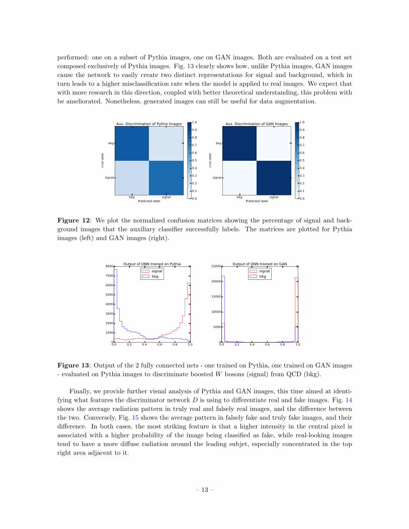
performed: one on a subset of Pythia images, one on GAN images. Both are evaluated on a test set

composed exclusively of Pythia images. Fig. 13 clearly shows how, unlike Pythia images, GAN images

cause the network to easily create two distinct representations for signal and background, which in

turn leads to a higher misclassification rate when the model is applied to real images. We expect that

with more research in this direction, coupled with better theoretical understanding, this problem with

be ameliorated. Nonetheless, generated images can still be useful for data augmentation.

bkg signalPredicted label

bkg

signal

Tru

e label

Aux. Discrimination of Pythia Images

0.0

0.1

0.2

0.3

0.4

0.5

0.6

0.7

0.8

0.9

1.0

bkg signalPredicted label

bkg

signal

Tru

e label

Aux. Discrimination of GAN Images

0.0

0.1

0.2

0.3

0.4

0.5

0.6

0.7

0.8

0.9

1.0

Figure 12: We plot the normalized confusion matrices showing the percentage of signal and back-

ground images that the auxiliary classifier successfully labels. The matrices are plotted for Pythia

images (left) and GAN images (right).

0.0 0.2 0.4 0.6 0.8 1.00

1000

2000

3000

4000

5000

6000

7000

8000Output of DNN trained on Pythia

signal

bkg

0.0 0.2 0.4 0.6 0.8 1.00

5000

10000

15000

20000

25000Output of DNN trained on GAN

signal

bkg

Figure 13: Output of the 2 fully connected nets - one trained on Pythia, one trained on GAN images

- evaluated on Pythia images to discriminate boosted W bosons (signal) from QCD (bkg).

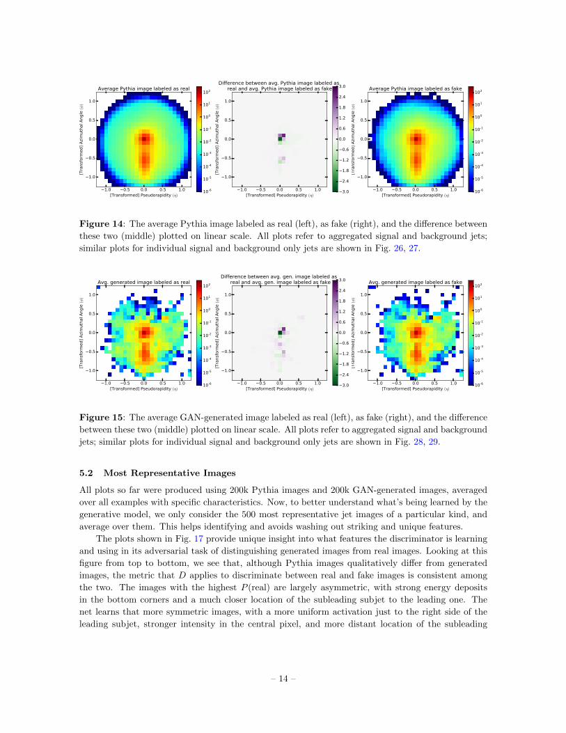
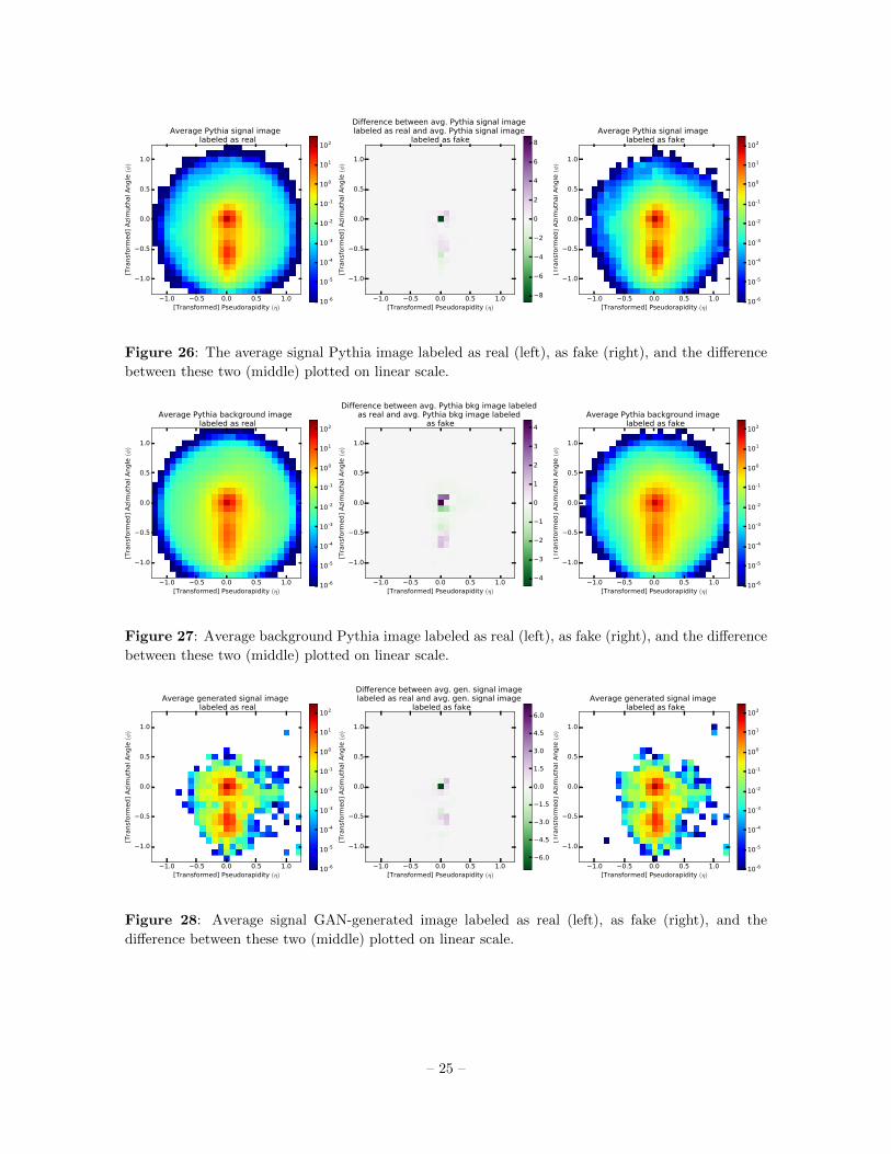
Finally, we provide further visual analysis of Pythia and GAN images, this time aimed at identi-

fying what features the discriminator network D is using to differentiate real and fake images. Fig. 14

shows the average radiation pattern in truly real and falsely real images, and the difference between

the two. Conversely, Fig. 15 shows the average pattern in falsely fake and truly fake images, and their

difference. In both cases, the most striking feature is that a higher intensity in the central pixel is

associated with a higher probability of the image being classified as fake, while real-looking images

tend to have a more diffuse radiation around the leading subjet, especially concentrated in the top

right area adjacent to it.

– 13 –


1.0

0.5

0.0

0.5

1.0

[Tra

nsf

orm

ed]

Azi

muth

al A

ngle

(φ)

Average Pythia image labeled as real

10-6

10-5

10-4

10-3

10-2

10-1

100

101

102


1.0

0.5

0.0

0.5

1.0

[Tra

nsf

orm

ed]

Azi

muth

al A

ngle

(φ)

Difference between avg. Pythia image labeled as real and avg. Pythia image labeled as fake

3.0

2.4

1.8

1.2

0.6

0.0

0.6

1.2

1.8

2.4

3.0


1.0

0.5

0.0

0.5

1.0

[Tra

nsf

orm

ed]

Azi

muth

al A

ngle

(φ)

Average Pythia image labeled as fake

10-6

10-5

10-4

10-3

10-2

10-1

100

101

102

Figure 14: The average Pythia image labeled as real (left), as fake (right), and the difference between

these two (middle) plotted on linear scale. All plots refer to aggregated signal and background jets;

similar plots for individual signal and background only jets are shown in Fig. 26, 27.


1.0

0.5

0.0

0.5

1.0

[Tra

nsf

orm

ed]

Azi

muth

al A

ngle

(φ)

Avg. generated image labeled as real

10-6

10-5

10-4

10-3

10-2

10-1

100

101

102


1.0

0.5

0.0

0.5

1.0

[Tra

nsf

orm

ed]

Azi

muth

al A

ngle

(φ)

Difference between avg. gen. image labeled as real and avg. gen. image labeled as fake

3.0

2.4

1.8

1.2

0.6

0.0

0.6

1.2

1.8

2.4

3.0


1.0

0.5

0.0

0.5

1.0

[Tra

nsf

orm

ed]

Azi

muth

al A

ngle

(φ)

Avg. generated image labeled as fake

10-6

10-5

10-4

10-3

10-2

10-1

100

101

102

Figure 15: The average GAN-generated image labeled as real (left), as fake (right), and the difference

between these two (middle) plotted on linear scale. All plots refer to aggregated signal and background

jets; similar plots for individual signal and background only jets are shown in Fig. 28, 29.

5.2 Most Representative Images

All plots so far were produced using 200k Pythia images and 200k GAN-generated images, averaged

over all examples with specific characteristics. Now, to better understand what’s being learned by the

generative model, we only consider the 500 most representative jet images of a particular kind, and

average over them. This helps identifying and avoids washing out striking and unique features.

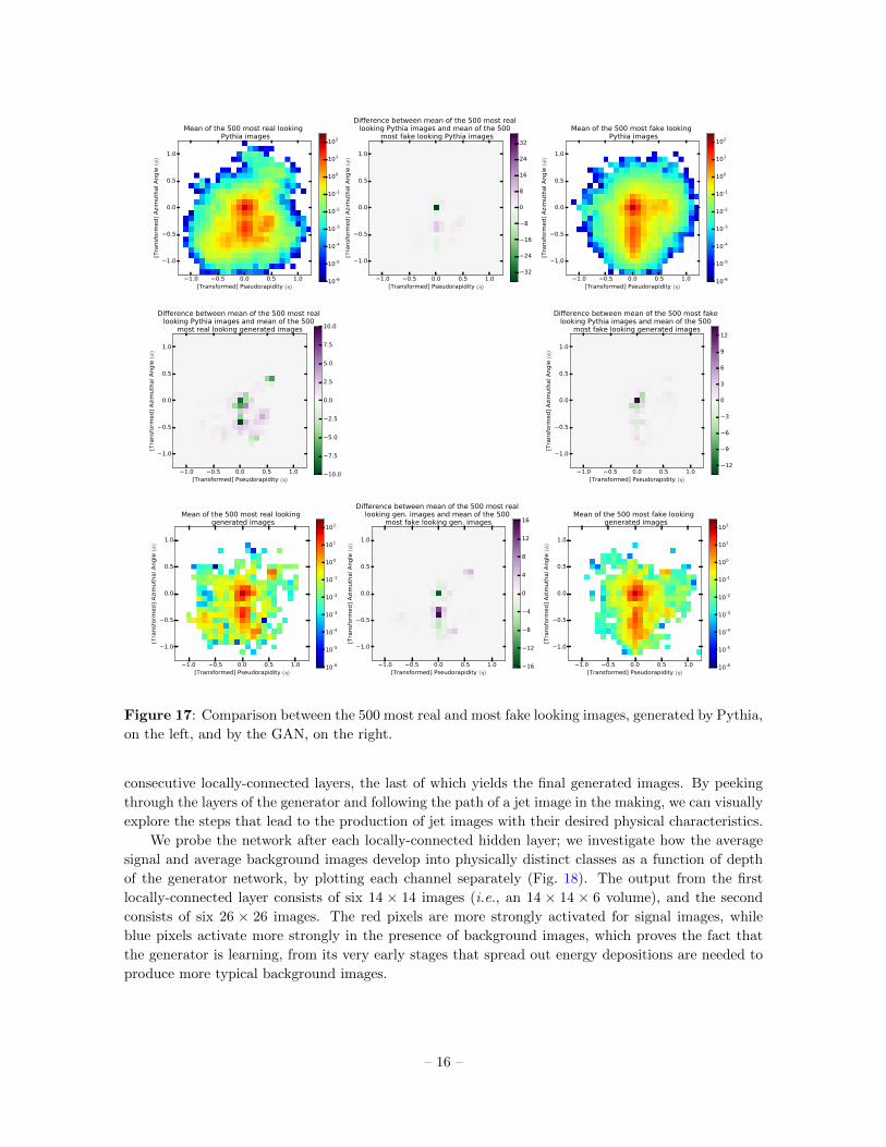
The plots shown in Fig. 17 provide unique insight into what features the discriminator is learning

and using in its adversarial task of distinguishing generated images from real images. Looking at this

figure from top to bottom, we see that, although Pythia images qualitatively differ from generated

images, the metric that D applies to discriminate between real and fake images is consistent among

the two. The images with the highest P (real) are largely asymmetric, with strong energy deposits

in the bottom corners and a much closer location of the subleading subjet to the leading one. The

net learns that more symmetric images, with a more uniform activation just to the right side of the

leading subjet, stronger intensity in the central pixel, and more distant location of the subleading

– 14 –

subjet, appear to be easier to produce for G and are therefore more easily identifiable as fake.


1.0

0.5

0.0

0.5

1.0

[Tra

nsf

orm

ed]

Azi

muth

al A

ngle

(φ)

Mean of the 500 most signal looking Pythia images

10-6

10-5

10-4

10-3

10-2

10-1

100

101

102


1.0

0.5

0.0

0.5

1.0

[Tra

nsf

orm

ed]

Azi

muth

al A

ngle

(φ)

Difference between mean of the 500 most signal looking Pythia images and mean of the 500

most bkg looking Pythia images

32

24

16

8

0

8

16

24

32


1.0

0.5

0.0

0.5

1.0

[Tra

nsf

orm

ed]

Azi

muth

al A

ngle

(φ)

Mean of the 500 most bkg looking Pythia images

10-6

10-5

10-4

10-3

10-2

10-1

100

101

102


1.0

0.5

0.0

0.5

1.0

[Tra

nsf

orm

ed]

Azi

muth

al A

ngle

(φ)

Difference between mean of the 500 most signal looking Pythia images and mean of the 500

most signal looking gen. images

6.0

4.5

3.0

1.5

0.0

1.5

3.0

4.5

6.0


1.0

0.5

0.0

0.5

1.0

[Tra

nsf

orm

ed]

Azi

muth

al A

ngle

(φ)

Difference between mean of the 500 most bkg looking Pythia images and mean of the 500

most bkg looking gen. images

12

9

6

3

0

3

6

9

12


1.0

0.5

0.0

0.5

1.0

[Tra

nsf

orm

ed]

Azi

muth

al A

ngle

(φ)

Mean of the 500 most signal looking generated images

10-6

10-5

10-4

10-3

10-2

10-1

100

101

102


1.0

0.5

0.0

0.5

1.0

[Tra

nsf

orm

ed]

Azi

muth

al A

ngle

(φ)

Difference between mean of the 500 most signal looking gen. images and mean of the

500 most bkg looking gen. images

16

12

8

4

0

4

8

12

16


1.0

0.5

0.0

0.5

1.0

[Tra

nsf

orm

ed]

Azi

muth

al A

ngle

(φ)

Mean of the 500 most bkg looking generated images

10-6

10-5

10-4

10-3

10-2

10-1

100

101

102

Figure 16: Comparison between the 500 most signal and most background looking images, generated

by Pythia, on the left, and by the GAN, on the right.

In addition, we can isolate the primary information that D pays attention to when classifying

signal and background images. The learned metric is consistently applied to both Pythia and GAN

images, as shown in Fig. 16. When identifying signal images, D learns to looks for more concentrated

images, with well-defined two prong structure. On the other hand, the network has learned that

background images have a wider radiation pattern and a more fuzzy structure around the location of

the second subjet.

5.3 Generator

To further understand the generation process of jet images using GANs, we explore the inner workings

of the generator network. As outlined in Sec. 4.1, G consists of a 2D convolution followed by 3

– 15 –


1.0

0.5

0.0

0.5

1.0[T

ransf

orm

ed]

Azi

muth

al A

ngle

(φ)

Mean of the 500 most real looking Pythia images

10-6

10-5

10-4

10-3

10-2

10-1

100

101

102


1.0

0.5

0.0

0.5

1.0

[Tra

nsf

orm

ed]

Azi

muth

al A

ngle

(φ)

Difference between mean of the 500 most real looking Pythia images and mean of the 500

most fake looking Pythia images

32

24

16

8

0

8

16

24

32


1.0

0.5

0.0

0.5

1.0

[Tra

nsf

orm

ed]

Azi

muth

al A

ngle

(φ)

Mean of the 500 most fake looking Pythia images

10-6

10-5

10-4

10-3

10-2

10-1

100

101

102


1.0

0.5

0.0

0.5

1.0

[Tra

nsf

orm

ed]

Azi

muth

al A

ngle

(φ)

Difference between mean of the 500 most real looking Pythia images and mean of the 500

most real looking generated images

10.0

7.5

5.0

2.5

0.0

2.5

5.0

7.5

10.0


1.0

0.5

0.0

0.5

1.0

[Tra

nsf

orm

ed]

Azi

muth

al A

ngle

(φ)

Difference between mean of the 500 most fake looking Pythia images and mean of the 500

most fake looking generated images

12

9

6

3

0

3

6

9

12


1.0

0.5

0.0

0.5

1.0

[Tra

nsf

orm

ed]

Azi

muth

al A

ngle

(φ)

Mean of the 500 most real looking generated images

10-6

10-5

10-4

10-3

10-2

10-1

100

101

102


1.0

0.5

0.0

0.5

1.0

[Tra

nsf

orm

ed]

Azi

muth

al A

ngle

(φ)

Difference between mean of the 500 most real looking gen. images and mean of the 500

most fake looking gen. images

16

12

8

4

0

4

8

12

16


1.0

0.5

0.0

0.5

1.0[T

ransf

orm

ed]

Azi

muth

al A

ngle

(φ)

Mean of the 500 most fake looking generated images

10-6

10-5

10-4

10-3

10-2

10-1

100

101

102

Figure 17: Comparison between the 500 most real and most fake looking images, generated by Pythia,

on the left, and by the GAN, on the right.

consecutive locally-connected layers, the last of which yields the final generated images. By peeking

through the layers of the generator and following the path of a jet image in the making, we can visually

explore the steps that lead to the production of jet images with their desired physical characteristics.

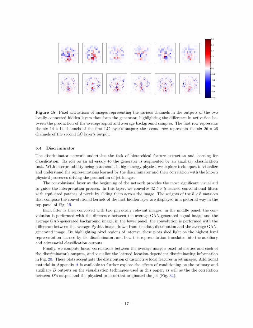
We probe the network after each locally-connected hidden layer; we investigate how the average

signal and average background images develop into physically distinct classes as a function of depth

of the generator network, by plotting each channel separately (Fig. 18). The output from the first

locally-connected layer consists of six 14 × 14 images (i.e., an 14 × 14 × 6 volume), and the second

consists of six 26 × 26 images. The red pixels are more strongly activated for signal images, while

blue pixels activate more strongly in the presence of background images, which proves the fact that

the generator is learning, from its very early stages that spread out energy depositions are needed to

produce more typical background images.

– 16 –

0.5

0.4

0.3

0.2

0.1

0.0

0.1

0.2

0.3

0.4

0.5

Figure 18: Pixel activations of images representing the various channels in the outputs of the two

locally-connected hidden layers that form the generator, highlighting the difference in activation be-

tween the production of the average signal and average background samples. The first row represents

the six 14 × 14 channels of the first LC layer’s output; the second row represents the six 26 × 26

channels of the second LC layer’s output.

5.4 Discriminator

The discriminator network undertakes the task of hierarchical feature extraction and learning for

classification. Its role as an adversary to the generator is augmented by an auxiliary classification

task. With interpretability being paramount in high energy physics, we explore techniques to visualize

and understand the representations learned by the discriminator and their correlation with the known

physical processes driving the production of jet images.

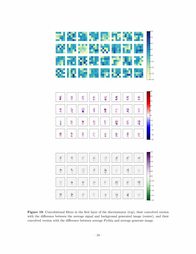
The convolutional layer at the beginning of the network provides the most significant visual aid

to guide the interpretation process. In this layer, we convolve 32 5 × 5 learned convolutional filters

with equi-sized patches of pixels by sliding them across the image. The weights of the 5× 5 matrices

that compose the convolutional kernels of the first hidden layer are displayed in a pictorial way in the

top panel of Fig. 19.

Each filter is then convolved with two physically relevant images: in the middle panel, the con-

volution is performed with the difference between the average GAN-generated signal image and the

average GAN-generated background image; in the lower panel, the convolution is performed with the

difference between the average Pythia image drawn from the data distribution and the average GAN-

generated image. By highlighting pixel regions of interest, these plots shed light on the highest level

representation learned by the discriminator, and how this representation translates into the auxiliary

and adversarial classification outputs.

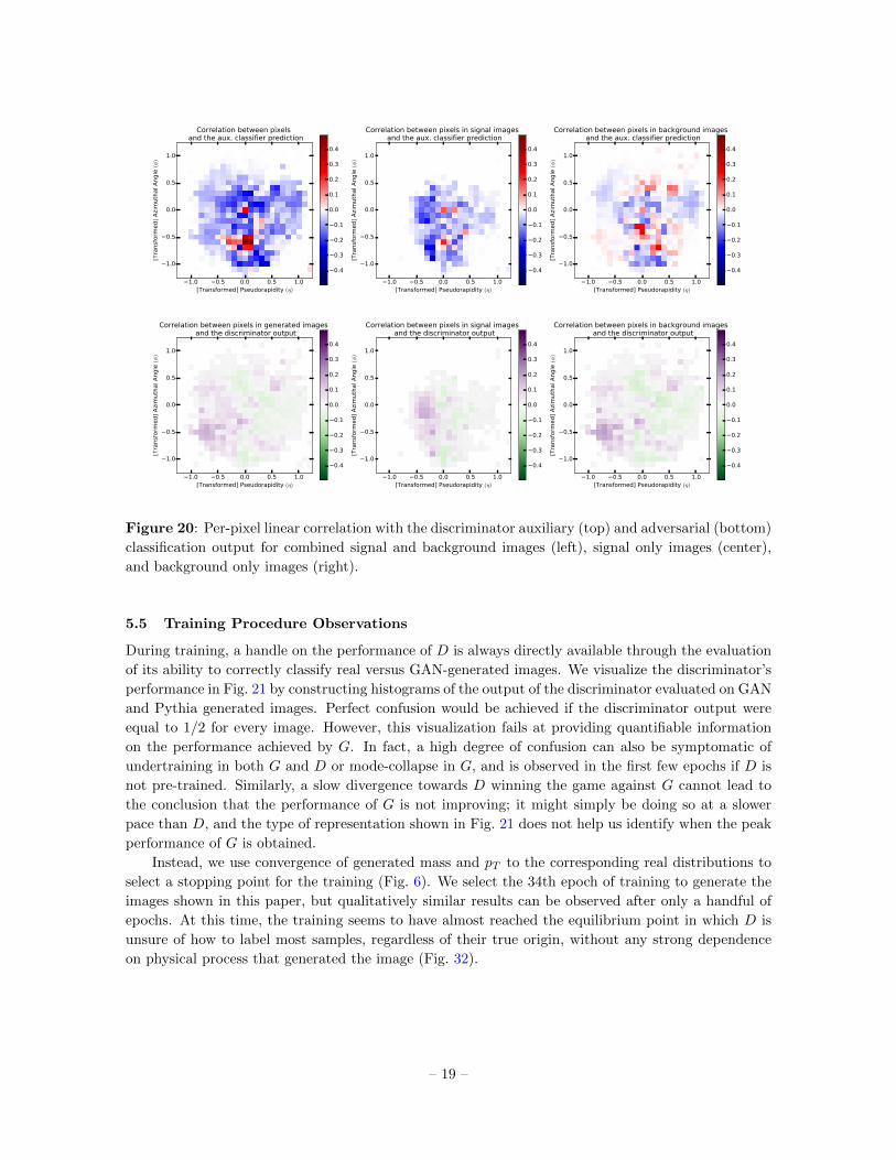
Finally, we compute linear correlations between the average image’s pixel intensities and each of

the discriminator’s outputs, and visualize the learned location-dependent discriminating information

in Fig. 20. These plots accentuate the distribution of distinctive local features in jet images. Additional

material in Appendix A is available to further explore the effects of conditioning on the primary and

auxiliary D outputs on the visualization techniques used in this paper, as well as the the correlation

between D’s output and the physical process that originated the jet (Fig. 32).

– 17 –

0.4

0.3

0.2

0.1

0.0

0.1

0.2

0.3

0.4

20

16

12

8

4

0

4

8

12

16

20

3.0

2.4

1.8

1.2

0.6

0.0

0.6

1.2

1.8

2.4

3.0

Figure 19: Convolutional filters in the first layer of the discriminator (top), their convolved version

with the difference between the average signal and background generated image (center), and their

convolved version with the difference between average Pythia and average generate image.

– 18 –


1.0

0.5

0.0

0.5

1.0[T

ransf

orm

ed]

Azi

muth

al A

ngle

(φ)

Correlation between pixels and the aux. classifier prediction

0.4

0.3

0.2

0.1

0.0

0.1

0.2

0.3

0.4


1.0

0.5

0.0

0.5

1.0

[Tra

nsf

orm

ed]

Azi

muth

al A

ngle

(φ)

Correlation between pixels in signal images and the aux. classifier prediction

0.4

0.3

0.2

0.1

0.0

0.1

0.2

0.3

0.4


1.0

0.5

0.0

0.5

1.0

[Tra

nsf

orm

ed]

Azi

muth

al A

ngle

(φ)

Correlation between pixels in background images and the aux. classifier prediction

0.4

0.3

0.2

0.1

0.0

0.1

0.2

0.3

0.4


1.0

0.5

0.0

0.5

1.0

[Tra

nsf

orm

ed]

Azi

muth

al A

ngle

(φ)

Correlation between pixels in generated images and the discriminator output

0.4

0.3

0.2

0.1

0.0

0.1

0.2

0.3

0.4


1.0

0.5

0.0

0.5

1.0[T

ransf

orm

ed]

Azi

muth

al A

ngle

(φ)

Correlation between pixels in signal images and the discriminator output

0.4

0.3

0.2

0.1

0.0

0.1

0.2

0.3

0.4


1.0

0.5

0.0

0.5

1.0

[Tra

nsf

orm

ed]

Azi

muth

al A

ngle

(φ)

Correlation between pixels in background images and the discriminator output

0.4

0.3

0.2

0.1

0.0

0.1

0.2

0.3

0.4

Figure 20: Per-pixel linear correlation with the discriminator auxiliary (top) and adversarial (bottom)

classification output for combined signal and background images (left), signal only images (center),

and background only images (right).

5.5 Training Procedure Observations

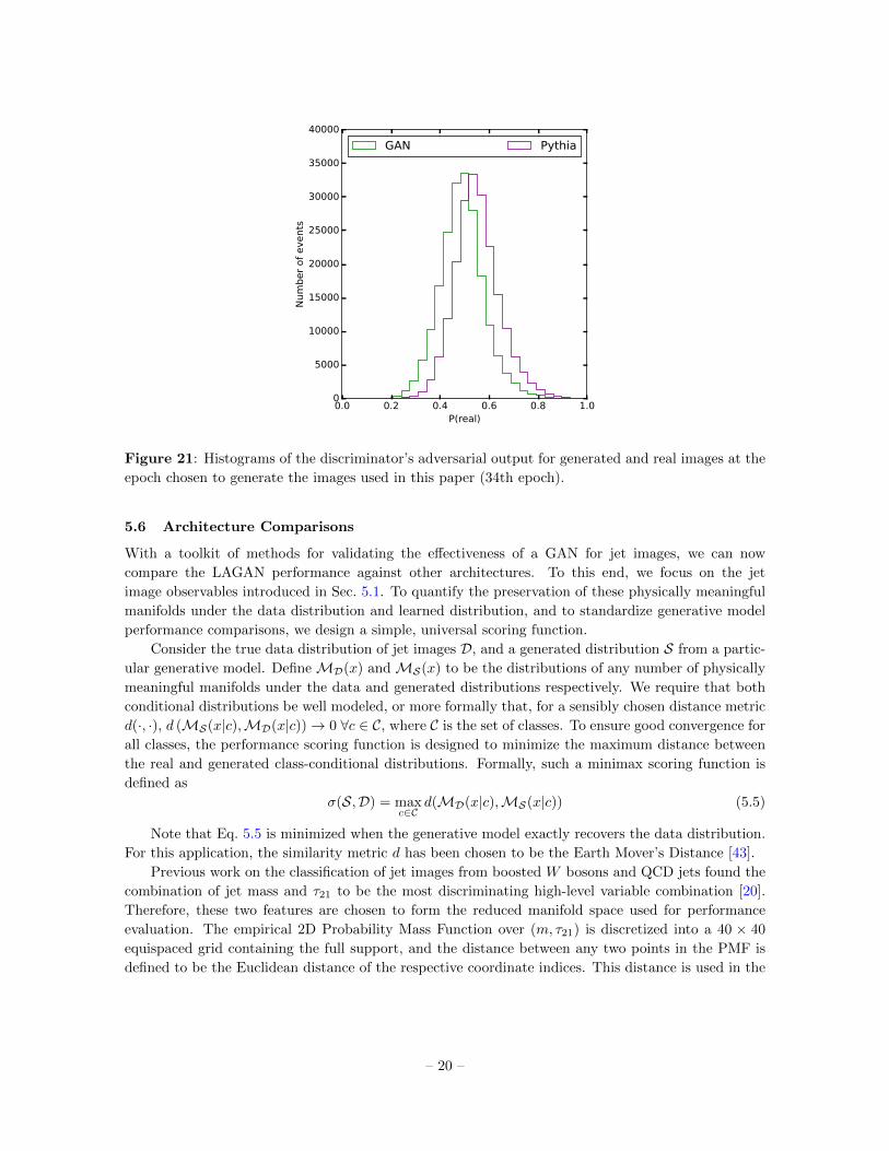
During training, a handle on the performance of D is always directly available through the evaluation

of its ability to correctly classify real versus GAN-generated images. We visualize the discriminator’s

performance in Fig. 21 by constructing histograms of the output of the discriminator evaluated on GAN

and Pythia generated images. Perfect confusion would be achieved if the discriminator output were

equal to 1/2 for every image. However, this visualization fails at providing quantifiable information

on the performance achieved by G. In fact, a high degree of confusion can also be symptomatic of

undertraining in both G and D or mode-collapse in G, and is observed in the first few epochs if D is

not pre-trained. Similarly, a slow divergence towards D winning the game against G cannot lead to

the conclusion that the performance of G is not improving; it might simply be doing so at a slower

pace than D, and the type of representation shown in Fig. 21 does not help us identify when the peak

performance of G is obtained.

Instead, we use convergence of generated mass and pT to the corresponding real distributions to

select a stopping point for the training (Fig. 6). We select the 34th epoch of training to generate the

images shown in this paper, but qualitatively similar results can be observed after only a handful of

epochs. At this time, the training seems to have almost reached the equilibrium point in which D is

unsure of how to label most samples, regardless of their true origin, without any strong dependence

on physical process that generated the image (Fig. 32).

– 19 –

0.0 0.2 0.4 0.6 0.8 1.0P(real)

0

5000

10000

15000

20000

25000

30000

35000

40000

Num

ber

of

events

GAN Pythia

Figure 21: Histograms of the discriminator’s adversarial output for generated and real images at the

epoch chosen to generate the images used in this paper (34th epoch).

5.6 Architecture Comparisons

With a toolkit of methods for validating the effectiveness of a GAN for jet images, we can now

compare the LAGAN performance against other architectures. To this end, we focus on the jet

image observables introduced in Sec. 5.1. To quantify the preservation of these physically meaningful

manifolds under the data distribution and learned distribution, and to standardize generative model

performance comparisons, we design a simple, universal scoring function.

Consider the true data distribution of jet images D, and a generated distribution S from a partic-

ular generative model. DefineMD(x) andMS(x) to be the distributions of any number of physically

meaningful manifolds under the data and generated distributions respectively. We require that both

conditional distributions be well modeled, or more formally that, for a sensibly chosen distance metric

d(·, ·), d (MS(x|c),MD(x|c))→ 0 ∀c ∈ C, where C is the set of classes. To ensure good convergence for

all classes, the performance scoring function is designed to minimize the maximum distance between

the real and generated class-conditional distributions. Formally, such a minimax scoring function is

defined as

σ(S,D) = maxc∈C

d(MD(x|c),MS(x|c)) (5.5)

Note that Eq. 5.5 is minimized when the generative model exactly recovers the data distribution.

For this application, the similarity metric d has been chosen to be the Earth Mover’s Distance [43].

Previous work on the classification of jet images from boosted W bosons and QCD jets found the

combination of jet mass and τ21 to be the most discriminating high-level variable combination [20].

Therefore, these two features are chosen to form the reduced manifold space used for performance

evaluation. The empirical 2D Probability Mass Function over (m, τ21) is discretized into a 40 × 40

equispaced grid containing the full support, and the distance between any two points in the PMF is

defined to be the Euclidean distance of the respective coordinate indices. This distance is used in the

– 20 –

internal flow optimization procedure when calculating the Earth Mover’s Distance. The two classes

are jets produced from boosted W boson decays and generic quark and gluon jets.

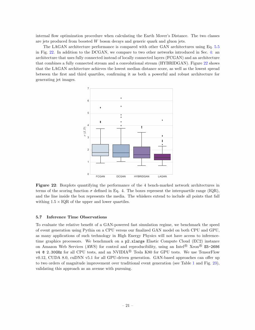
The LAGAN architecture performance is compared with other GAN architectures using Eq. 5.5

in Fig. 22. In addition to the DCGAN, we compare to two other networks introduced in Sec. 4: an

architecture that uses fully connected instead of locally connected layers (FCGAN) and an architecture

that combines a fully connected stream and a convolutional stream (HYBRIDGAN). Figure 22 shows

that the LAGAN architecture achieves the lowest median distance score, as well as the lowest spread

between the first and third quartiles, confirming it as both a powerful and robust architecture for

generating jet images.

FCGAN DCGAN HYBRIDGAN LAGAN0

1

2

3

4

5

6

7σ

(S,D

)

Figure 22: Boxplots quantifying the performance of the 4 bench-marked network architectures in

terms of the scoring function σ defined in Eq. 4. The boxes represent the interquartile range (IQR),

and the line inside the box represents the media. The whiskers extend to include all points that fall

withing 1.5× IQR of the upper and lower quartiles.

5.7 Inference Time Observations

To evaluate the relative benefit of a GAN-powered fast simulation regime, we benchmark the speed

of event generation using Pythia on a CPU versus our finalized GAN model on both CPU and GPU,

as many applications of such technology in High Energy Physics will not have access to inference-

time graphics processors. We benchmark on a p2.xlarge Elastic Compute Cloud (EC2) instance

on Amazon Web Services (AWS) for control and reproducibility, using an Intel R© Xeon R© E5-2686

v4 @ 2.30GHz for all CPU tests, and an NVIDIA R© Tesla K80 for GPU tests. We use TensorFlow

v0.12, CUDA 8.0, cuDNN v5.1 for all GPU-driven generation. GAN-based approaches can offer up

to two orders of magnitude improvement over traditional event generation (see Table 1 and Fig. 23),

validating this approach as an avenue with pursuing.

– 21 –

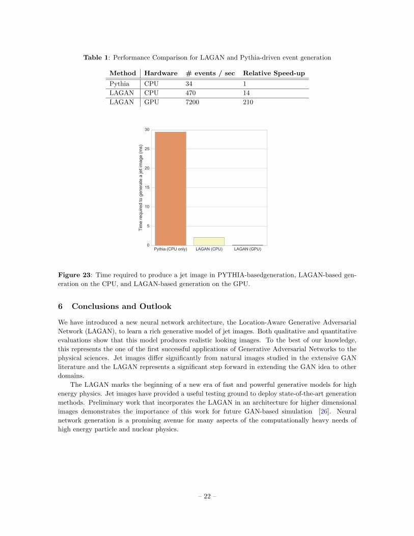
Table 1: Performance Comparison for LAGAN and Pythia-driven event generation

Method Hardware # events / sec Relative Speed-up

Pythia CPU 34 1

LAGAN CPU 470 14

LAGAN GPU 7200 210

Pythia (CPU only) LAGAN (CPU) LAGAN (GPU)0

5

10

15

20

25

30

Tim

e re

quire

d to

gen

erat

e a

jet i

mag

e (m

s)

Figure 23: Time required to produce a jet image in PYTHIA-basedgeneration, LAGAN-based gen-

eration on the CPU, and LAGAN-based generation on the GPU.

6 Conclusions and Outlook

We have introduced a new neural network architecture, the Location-Aware Generative Adversarial

Network (LAGAN), to learn a rich generative model of jet images. Both qualitative and quantitative

evaluations show that this model produces realistic looking images. To the best of our knowledge,

this represents the one of the first successful applications of Generative Adversarial Networks to the

physical sciences. Jet images differ significantly from natural images studied in the extensive GAN

literature and the LAGAN represents a significant step forward in extending the GAN idea to other

domains.

The LAGAN marks the beginning of a new era of fast and powerful generative models for high

energy physics. Jet images have provided a useful testing ground to deploy state-of-the-art generation

methods. Preliminary work that incorporates the LAGAN in an architecture for higher dimensional

images demonstrates the importance of this work for future GAN-based simulation [26]. Neural

network generation is a promising avenue for many aspects of the computationally heavy needs of

high energy particle and nuclear physics.

– 22 –

Acknowledgements

This work was supported in part by the Office of High Energy Physics of the U.S. Department of

Energy under contracts DE-AC02-05CH11231 and DE-FG02-92ER40704. The authors would like to

thank Ian Goodfellow for insightful deep learning related discussion, and would like to acknowledge

Wahid Bhimji, Zach Marshall, Mustafa Mustafa, Chase Shimmin, and Paul Tipton, who helped refine

our narrative.

– 23 –

A Additional Material


1.0

0.5

0.0

0.5

1.0

[Tra

nsf

orm

ed]

Azi

muth

al A

ngle

(φ)

10-6

10-5

10-4

10-3

10-2

10-1

100

101

102

Pix

el pT (

GeV

)


1.0

0.5

0.0

0.5

1.0

[Tra

nsf

orm

ed]

Azi

muth

al A

ngle

(φ)

Difference between avg. Pythia signal image and avg. generated signal image

3.2

2.4

1.6

0.8

0.0

0.8

1.6

2.4

3.2


1.0

0.5

0.0

0.5

1.0

[Tra

nsf

orm

ed]

Azi

muth

al A

ngle

(φ)

Average generated signal image

10-6

10-5

10-4

10-3

10-2

10-1

100

101

102

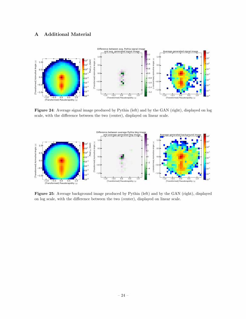
Figure 24: Average signal image produced by Pythia (left) and by the GAN (right), displayed on log

scale, with the difference between the two (center), displayed on linear scale.


1.0

0.5

0.0

0.5

1.0

[Tra

nsf

orm

ed]

Azi

muth

al A

ngle

(φ)

10-6

10-5

10-4

10-3

10-2

10-1

100

101

102

Pix

el pT (

GeV

)


1.0

0.5

0.0

0.5

1.0

[Tra

nsf

orm

ed]

Azi

muth

al A

ngle

(φ)

Difference between average Pythia bkg image and average generated bkg image

6

4

2

0

2

4

6


1.0

0.5

0.0

0.5

1.0

[Tra

nsf

orm

ed]

Azi

muth

al A

ngle

(φ)

Average generated background image

10-6

10-5

10-4

10-3

10-2

10-1

100

101

102

Figure 25: Average background image produced by Pythia (left) and by the GAN (right), displayed

on log scale, with the difference between the two (center), displayed on linear scale.

– 24 –


1.0

0.5

0.0

0.5

1.0

[Tra

nsf

orm

ed]

Azi

muth

al A

ngle

(φ)

Average Pythia signal image labeled as real

10-6

10-5

10-4

10-3

10-2

10-1

100

101

102


1.0

0.5

0.0

0.5

1.0

[Tra

nsf

orm

ed]

Azi

muth

al A

ngle

(φ)

Difference between avg. Pythia signal image labeled as real and avg. Pythia signal image

labeled as fake

8

6

4

2

0

2

4

6

8


1.0

0.5

0.0

0.5

1.0

[Tra

nsf

orm

ed]

Azi

muth

al A

ngle

(φ)

Average Pythia signal image labeled as fake

10-6

10-5

10-4

10-3

10-2

10-1

100

101

102

Figure 26: The average signal Pythia image labeled as real (left), as fake (right), and the difference

between these two (middle) plotted on linear scale.


1.0

0.5

0.0

0.5

1.0

[Tra

nsf

orm

ed]

Azi

muth

al A

ngle

(φ)

Average Pythia background image labeled as real

10-6

10-5

10-4

10-3

10-2

10-1

100

101

102


1.0

0.5

0.0

0.5

1.0

[Tra

nsf

orm

ed]

Azi

muth

al A

ngle

(φ)

Difference between avg. Pythia bkg image labeled as real and avg. Pythia bkg image labeled

as fake

4

3

2

1

0

1

2

3

4


1.0

0.5

0.0

0.5

1.0

[Tra

nsf

orm

ed]

Azi

muth

al A

ngle

(φ)

Average Pythia background image labeled as fake

10-6

10-5

10-4

10-3

10-2

10-1

100

101

102

Figure 27: Average background Pythia image labeled as real (left), as fake (right), and the difference

between these two (middle) plotted on linear scale.


1.0

0.5

0.0

0.5

1.0

[Tra

nsf

orm

ed]

Azi

muth

al A

ngle

(φ)

Average generated signal image labeled as real

10-6

10-5

10-4

10-3

10-2

10-1

100

101

102


1.0

0.5

0.0

0.5

1.0

[Tra

nsf

orm

ed]

Azi

muth

al A

ngle

(φ)

Difference between avg. gen. signal image labeled as real and avg. gen. signal image

labeled as fake

6.0

4.5

3.0

1.5

0.0

1.5

3.0

4.5

6.0


1.0

0.5

0.0

0.5

1.0

[Tra

nsf

orm

ed]

Azi

muth

al A

ngle

(φ)

Average generated signal image labeled as fake

10-6

10-5

10-4

10-3

10-2

10-1

100

101

102

Figure 28: Average signal GAN-generated image labeled as real (left), as fake (right), and the

difference between these two (middle) plotted on linear scale.

– 25 –


1.0

0.5

0.0

0.5

1.0

[Tra

nsf

orm

ed]

Azi

muth

al A

ngle

(φ)

Average generated background image labeled as real

10-6

10-5

10-4

10-3

10-2

10-1

100

101

102


1.0

0.5

0.0

0.5

1.0

[Tra

nsf

orm

ed]

Azi

muth

al A

ngle

(φ)

Difference between avg. gen. bkg image labeled as real and avg. gen. bkg image

labeled as fake

3.2

2.4

1.6

0.8

0.0

0.8

1.6

2.4

3.2


1.0

0.5

0.0

0.5

1.0

[Tra

nsf

orm

ed]

Azi

muth

al A

ngle

(φ)

Average generated background image labeled as fake

10-6

10-5

10-4

10-3

10-2

10-1

100

101

102

Figure 29: Average background GAN-generated image labeled as real (left), as fake (right), and the

difference between these two (middle) plotted on linear scale.


1.0

0.5

0.0

0.5

1.0

[Tra

nsf

orm

ed]

Azi

muth

al A

ngle

(φ)

Difference between avg. Pythia signal image labeled as real and avg. Pythia background image

labeled as real

12

9

6

3

0

3

6

9

12


1.0

0.5

0.0

0.5

1.0

[Tra

nsf

orm

ed]

Azi

muth

al A

ngle

(φ)

Difference between avg. gen. signal image labeled as real and avg. gen. bkg image

labeled as real

20

15

10

5

0

5

10

15

20

Figure 30: Difference between the average signal and the average background images labeled as real,

produced by Pythia (left) and by the GAN (right), both displayed on linear scale.


1.0

0.5

0.0

0.5

1.0

[Tra

nsf

orm

ed]

Azi

muth

al A

ngle

(φ)

Difference between avg. Pythia signal image labeled as fake and avg. Pythia background

image labeled as fake

24

18

12

6

0

6

12

18

24


1.0

0.5

0.0

0.5

1.0

[Tra

nsf

orm

ed]

Azi

muth

al A

ngle

(φ)

Difference between avg. gen. signal image labeled as fake and avg. gen. bkg image

labeled as fake

24

16

8

0

8

16

24

Figure 31: Difference between the average signal and the average background images labeled as fake,

produced by Pythia (left) and by the GAN (right), both displayed on linear scale.

– 26 –

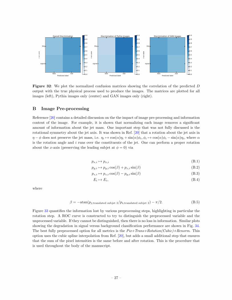
fake realPredicted label

bkg

signal

Tru

e label

Overall Discrimination

0.0

0.1

0.2

0.3

0.4

0.5

0.6

0.7

0.8

0.9

1.0


bkg

signal

Tru

e label

Discrimination of Pythia Images

0.0

0.1

0.2

0.3

0.4

0.5

0.6

0.7

0.8

0.9

1.0


bkg

signal

Tru

e label

Discrimination of GAN Images

0.0

0.1

0.2

0.3

0.4

0.5

0.6

0.7

0.8

0.9

1.0

Figure 32: We plot the normalized confusion matrices showing the correlation of the predicted D

output with the true physical process used to produce the images. The matrices are plotted for all

images (left), Pythia images only (center) and GAN images only (right).

B Image Pre-processing

Reference [20] contains a detailed discussion on the the impact of image pre-processing and information

content of the image. For example, it is shown that normalizing each image removes a significant

amount of information about the jet mass. One important step that was not fully discussed is the

rotational symmetry about the jet axis. It was shown in Ref. [20] that a rotation about the jet axis in

η− φ does not preserve the jet mass, i.e. ηi 7→ cos(α)ηi + sin(α)φi, φi 7→ cos(α)φi − sin(α)ηi, where α

is the rotation angle and i runs over the constituents of the jet. One can perform a proper rotation

about the x-axis (preserving the leading subjet at φ = 0) via

px,i 7→ px,i (B.1)

py,i 7→ py,i cos(β) + pz,i sin(β) (B.2)

pz,i 7→ pz,i cos(β)− py,i sin(β) (B.3)

Ei 7→ Ei, (B.4)

where

β = −atan(py,translated subjet 2/pz,translated subjet 2)− π/2. (B.5)

Figure 33 quantifies the information lost by various preprocessing steps, highlighting in particular the

rotation step. A ROC curve is constructed to try to distinguish the preprocessed variable and the

unprocessed variable. If they cannot be distinguished, then there is no loss in information. Similar plots

showing the degradation in signal versus background classification performance are shown in Fig. 34.

The best fully preprocessed option for all metrics is the Pix+Trans+Rotation(Cubic)+Renorm. This

option uses the cubic spline interpolation from Ref. [20], but adds a small additional step that ensures

that the sum of the pixel intensities is the same before and after rotation. This is the procedure that

is used throughout the body of the manuscript.

– 27 –

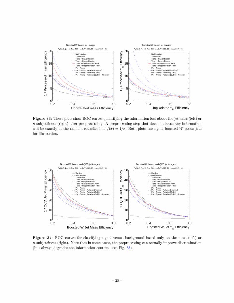
Unpixelated mass Efficiency0.2 0.4 0.6 0.8

1 / P

roce

ssed

mas

s E

ffici

ency

0

5

10

15

20No PixelationTranslationTrans + Naive RotationTrans + Proper RotationTrans + Naive Rotation + PixTrans + Proper Rotation + PixPix + TransPix + Trans + Rotation (Nearest)Pix + Trans + Rotation (Cubic)Pix + Trans + Rotation (Cubic) + Renorm

/GeV < 300, 65 < mass/GeV < 95T

= 13 TeV, 250 < psPythia 8,

Boosted W boson jet images

Efficiency21τUnpixelated 0.2 0.4 0.6 0.8

Effi

cien

cy21τ

1 / P

roce

ssed

0

5

10

15

20No PixelationTranslationTrans + Naive RotationTrans + Proper RotationTrans + Naive Rotation + PixTrans + Proper Rotation + PixPix + TransPix + Trans + Rotation (Nearest)Pix + Trans + Rotation (Cubic)Pix + Trans + Rotation (Cubic) + Renorm

/GeV < 300, 65 < mass/GeV < 95T


Boosted W boson jet images

Figure 33: These plots show ROC curves quantifying the information lost about the jet mass (left) or

n-subjettiness (right) after pre-processing. A preprocessing step that does not loose any information

will be exactly at the random classifier line f(x) = 1/x. Both plots use signal boosted W boson jets

for illustration.

Boosted W Jet Mass Efficiency0.2 0.4 0.6 0.8

1 / Q

CD

Jet

Mas

s E

ffici

ency

0

10

20

30

40

50RandomNo PixelationTranslationTrans + Naive RotationTrans + Proper RotationTrans + Naive Rotation + PixTrans + Proper Rotation + PixPix + TransPix + Trans + Rotation (Nearest)Pix + Trans + Rotation (Cubic)Pix + Trans + Rotation (Cubic) + Renorm

/GeV < 300, 65 < mass/GeV < 95T


Boosted W boson and QCD jet images

Efficiency21τBoosted W Jet 0.2 0.4 0.6 0.8

Effi

cien

cy21τ

1 / Q

CD

Jet

0

10

20

30

40

50RandomNo PixelationTranslationTrans + Naive RotationTrans + Proper RotationTrans + Naive Rotation + PixTrans + Proper Rotation + PixPix + TransPix + Trans + Rotation (Nearest)Pix + Trans + Rotation (Cubic)Pix + Trans + Rotation (Cubic) + Renorm

/GeV < 300, 65 < mass/GeV < 95T


Boosted W boson and QCD jet images

Figure 34: ROC curves for classifying signal versus background based only on the mass (left) or

n-subjettiness (right). Note that in some cases, the preprocessing can actually improve discrimination

(but always degrades the information content - see Fig. 33).

– 28 –

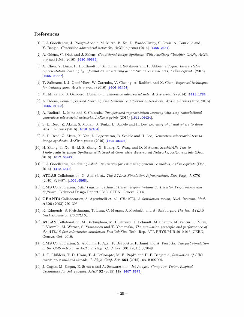
References

[1] I. J. Goodfellow, J. Pouget-Abadie, M. Mirza, B. Xu, D. Warde-Farley, S. Ozair, A. Courville and

Y. Bengio, Generative adversarial networks, ArXiv e-prints (2014) [1406.2661].

[2] A. Odena, C. Olah and J. Shlens, Conditional Image Synthesis With Auxiliary Classifier GANs, ArXiv

e-prints (Oct., 2016) [1610.09585].

[3] X. Chen, Y. Duan, R. Houthooft, J. Schulman, I. Sutskever and P. Abbeel, Infogan: Interpretable

representation learning by information maximizing generative adversarial nets, ArXiv e-prints (2016)

[1606.03657].

[4] T. Salimans, I. J. Goodfellow, W. Zaremba, V. Cheung, A. Radford and X. Chen, Improved techniques

for training gans, ArXiv e-prints (2016) [1606.03498].

[5] M. Mirza and S. Osindero, Conditional generative adversarial nets, ArXiv e-prints (2014) [1411.1784].

[6] A. Odena, Semi-Supervised Learning with Generative Adversarial Networks, ArXiv e-prints (June, 2016)

[1606.01583].

[7] A. Radford, L. Metz and S. Chintala, Unsupervised representation learning with deep convolutional

generative adversarial networks, ArXiv e-prints (2015) [1511.06434].

[8] S. E. Reed, Z. Akata, S. Mohan, S. Tenka, B. Schiele and H. Lee, Learning what and where to draw,

ArXiv e-prints (2016) [1610.02454].

[9] S. E. Reed, Z. Akata, X. Yan, L. Logeswaran, B. Schiele and H. Lee, Generative adversarial text to

image synthesis, ArXiv e-prints (2016) [1605.05396].

[10] H. Zhang, T. Xu, H. Li, S. Zhang, X. Huang, X. Wang and D. Metaxas, StackGAN: Text to

Photo-realistic Image Synthesis with Stacked Generative Adversarial Networks, ArXiv e-prints (Dec.,

2016) [1612.03242].

[11] I. J. Goodfellow, On distinguishability criteria for estimating generative models, ArXiv e-prints (Dec.,

2014) [1412.6515].

[12] ATLAS Collaboration, G. Aad et. al., The ATLAS Simulation Infrastructure, Eur. Phys. J. C70

(2010) 823–874 [1005.4568].

[13] CMS Collaboration, CMS Physics: Technical Design Report Volume 1: Detector Performance and

Software. Technical Design Report CMS. CERN, Geneva, 2006.

[14] GEANT4 Collaboration, S. Agostinelli et. al., GEANT4: A Simulation toolkit, Nucl. Instrum. Meth.

A506 (2003) 250–303.

[15] K. Edmonds, S. Fleischmann, T. Lenz, C. Magass, J. Mechnich and A. Salzburger, The fast ATLAS

track simulation (FATRAS), .

[16] ATLAS Collaboration, M. Beckingham, M. Duehrssen, E. Schmidt, M. Shapiro, M. Venturi, J. Virzi,

I. Vivarelli, M. Werner, S. Yamamoto and T. Yamanaka, The simulation principle and performance of

the ATLAS fast calorimeter simulation FastCaloSim, Tech. Rep. ATL-PHYS-PUB-2010-013, CERN,

Geneva, Oct, 2010.

[17] CMS Collaboration, S. Abdullin, P. Azzi, F. Beaudette, P. Janot and A. Perrotta, The fast simulation

of the CMS detector at LHC, J. Phys. Conf. Ser. 331 (2011) 032049.

[18] J. T. Childers, T. D. Uram, T. J. LeCompte, M. E. Papka and D. P. Benjamin, Simulation of LHC

events on a millions threads, J. Phys. Conf. Ser. 664 (2015), no. 9 092006.

[19] J. Cogan, M. Kagan, E. Strauss and A. Schwarztman, Jet-Images: Computer Vision Inspired

Techniques for Jet Tagging, JHEP 02 (2015) 118 [1407.5675].

– 29 –

http://arXiv.org/abs/1406.2661













[20] L. de Oliveira, M. Kagan, L. Mackey, B. Nachman and A. Schwartzman, Jet-images — deep learning

edition, JHEP 07 (2016) 069 [1511.05190].

[21] L. G. Almeida, M. Backovic, M. Cliche, S. J. Lee and M. Perelstein, Playing Tag with ANN: Boosted

Top Identification with Pattern Recognition, JHEP 07 (2015) 086 [1501.05968].

[22] P. T. Komiske, E. M. Metodiev and M. D. Schwartz, Deep learning in color: towards automated

quark/gluon jet discrimination, 1612.01551.

[23] J. Barnard, E. N. Dawe, M. J. Dolan and N. Rajcic, Parton Shower Uncertainties in Jet Substructure

Analyses with Deep Neural Networks, 1609.00607.

[24] P. Baldi, K. Bauer, C. Eng, P. Sadowski and D. Whiteson, Jet Substructure Classification in

High-Energy Physics with Deep Neural Networks, Phys. Rev. D93 (2016), no. 9 094034 [1603.09349].

[25] CMS Collaboration, S. Chatrchyan et. al., The CMS Experiment at the CERN LHC, JINST 3 (2008)

S08004.

[26] M. Paganini, L. de Oliveira and B. Nachman, CaloGAN: Simulating 3D High Energy Particle Showers

in Multi-Layer Electromagnetic Calorimeters with Generative Adversarial Networks, 1705.02355.

[27] M. Cacciari, G. P. Salam and G. Soyez JHEP 063.

[28] M. Cacciari, G. P. Salam and G. Soyez, FastJet User Manual, Eur. Phys. J. C72 (2012) 1896

[1111.6097].

[29] D. Krohn, J. Thaler and L.-T. Wang, Jet Trimming, JHEP 1002 (2010) 084 [0912.1342].

[30] T. Sjostrand, S. Mrenna and P. Z. Skands, A Brief Introduction to PYTHIA 8.1, Comput. Phys.

Commun. 178 (2008) 852–867 [0710.3820].

[31] T. Sjostrand, S. Mrenna and P. Z. Skands, PYTHIA 6.4 Physics and Manual, JHEP 0605 (2006) 026

[hep-ph/0603175].

[32] B. Nachman, L. de Oliveira and M. Paganini, Dataset release - Pythia generated jet images for location

aware generative adversarial network training, Feb., 2017. 10.17632/4r4v785rgx.1.

[33] L. de Oliveira and M. Paganini, lukedeo/adversarial-jets: Initial code release, Mar., 2017.

10.5281/zenodo.400708.

[34] A. L. Maas, A. Y. Hannun and A. Y. Ng, Rectifier nonlinearities improve neural network acoustic

models, in Proc. ICML, vol. 30, 2013.

[35] S. Chintala, How to train a GAN?, NIPS, Workshop on Generative Adversarial Networks (2016).

[36] A. L. Maas, A. Y. Hannun and A. Y. Ng, Rectifier Nonlinearities Improve Neural Network Acoustic

Models, .

[37] S. Ioffe and C. Szegedy, Batch normalization: Accelerating deep network training by reducing internal

covariate shift, 1502.03167.

[38] D. P. Kingma and J. Ba, Adam: A method for stochastic optimization, CoRR abs/1412.6980 (2014).

[39] F. Chollet, “Keras.” https://github.com/fchollet/keras, 2017.

[40] M. Abadi, A. Agarwal, P. Barham, E. Brevdo, Z. Chen, C. Citro, G. S. Corrado, A. Davis, J. Dean,

M. Devin, S. Ghemawat, I. Goodfellow, A. Harp, G. Irving, M. Isard, Y. Jia, R. Jozefowicz, L. Kaiser,

M. Kudlur, J. Levenberg, D. Mane, R. Monga, S. Moore, D. Murray, C. Olah, M. Schuster, J. Shlens,

B. Steiner, I. Sutskever, K. Talwar, P. Tucker, V. Vanhoucke, V. Vasudevan, F. Viegas, O. Vinyals,

P. Warden, M. Wattenberg, M. Wicke, Y. Yu and X. Zheng, TensorFlow: Large-scale machine learning

on heterogeneous systems, 2015. Software available from https://www.tensorflow.org/.

– 30 –










http://arXiv.org/abs/hep-ph/0603175

https://data.mendeley.com/datasets/4r4v785rgx/1

https://doi.org/10.5281/zenodo.400708


https://github.com/fchollet/keras

https://www.tensorflow.org/

[41] J. Thaler and K. Van Tilburg, Identifying Boosted Objects with N-subjettiness, JHEP 1103 (2011) 015

[1011.2268].

[42] A. J. Larkoski, D. Neill and J. Thaler, Jet Shapes with the Broadening Axis, JHEP 04 (2014) 017

[1401.2158].

[43] Y. Rubner, C. Tomasi and L. J. Guibas, The earth mover’s distance as a metric for image retrieval, Int.

J. Comput. Vision 40 (Nov., 2000) 99–121.

– 31 –



Documents

Learning Particle Physics by Example: Location-Aware ... · Learning Particle Physics by Example: Location-Aware Generative Adversarial Networks for Physics Synthesis ... simulations