Learning Semantic Features for Action Recognition via

Diffusion Maps

Jingen Liua, Yang Yang, Imran Saleemi and Mubarak Shahb

aDepartment of EECS, University of Michigan, Ann Arbor, MI, USAbDepartment of EECS, University of Central Florida, Orlando, FL, USA

Abstract

Efficient modeling of actions is critical for recognizing human actions. Re-

cently, bag of video words (BoVW) representation, in which features com-

puted around spatiotemporal interest points are quantized into video words

based on their appearance similarity, has been widely and successfully ex-

plored. The performance of this representation however, is highly sensitive

to two main factors: the granularity, and therefore, the size of vocabulary,

and the space in which features and words are clustered, i.e., the distance

measure between data points at different levels of the hierarchy. The goal

of this paper is to propose a representation and learning framework that

addresses both these limitations.

We present a principled approach to learning a semantic vocabulary from

a large amount of video words using diffusion maps embedding. As opposed

to flat vocabularies used in traditional methods, we propose to exploit the

hierarchical nature of feature vocabularies representative of human actions.

Spatiotemporal features computed around interest points in videos form the

lowest level of representation. Video words are then obtained by clustering

those spatiotemporal features. Each video word is then represented by a

Preprint submitted to Computer Vision and Image Understanding October 30, 2011

vector of pointwise mutual information (PMI) between that video word and

training video clips, and is treated as a mid-level feature. At the highest

level of the hierarchy, our goal is to further cluster the mid-level features,

while exploiting semantically meaningful distance measures between them.

We conjecture that the mid-level features produced by similar video sources

(action classes) must lie on a certain manifold. To capture the relationship

between these features, and retain it during clustering, we propose to use

diffusion distance as a measure of similarity between them. The underlying

idea is to embed the mid-level features into a lower-dimensional space, so

as to construct a compact yet discriminative, high level vocabulary. Unlike

some of the supervised vocabulary construction approaches and the unsu-

pervised methods such as pLSA and LDA, diffusion maps can capture local

relationship between the mid-level features on the manifold. We have tested

our approach on diverse datasets and have obtained very promising results.

Keywords:

Action Recognition, Bag of Video Words, Semantic Visual Vocabulary,

Diffusion Maps, Pointwise Mutual Information

1. Introduction

Recognition of human actions like “walking”, “boxing”, “horseback rid-

ing”, and “cycling”, etc. (Figure 1 (a)) is of critical importance in analysis of

the vast amount of visual data, including visual media, personal, and surveil-

lance videos, produced every day. Despite the large number of techniques and

algorithms proposed to solve this problem [10], human action recognition re-

mains a challenging problem due to camera motion, occlusion, illumination

2

changes, individual variations of object appearance and postures, and the

sheer diversity of such videos in general. In order to overcome these prob-

lems, a compact, discriminative, and semantically meaningful representation

(or vocabulary) must lie at the heart of any reasonable solution.

Representations of human actions proposed in the computer vision lit-

erature range from holistic, to part-based, to interest-point based local rep-

resentations, examples of which include learned geometrical models of the

human body parts [46, 45], space-time pattern templates [4, 19], shape or

form features [6, 41, 25, 1, 16], as well as motion or optical flow patterns

[39, 1]. Recently, the bag-of-features based representation has received in-

creased attention due to its computational simplicity and surprisingly good

performance. Inspired by the success of the bag-of-words (BoW) approach

in text categorization [9, 55], where a document is represented as a his-

togram of words, researchers have discovered the connection between local

spatiotemporal cuboids (3D patches) in videos and words in documents. In

order to employ the BoW mechanism for action representation, feature vec-

tors extracted from such cuboids need to be quantized into video words via

clustering algorithms such as k-means. An action video can be modelled as a

bag of video words (BoVW), namely a histogram of video words, which has

also been applied in early object recognition [17, 44].

The BoVW representation has the potential to overcome several com-

monly encountered problems in human action recognition. This representa-

tion captures local information, as opposed to holistic or part-based represen-

tations, because it models actions as histogram of video words, where each

video word represents a small spatiotemporal region of the video. Although

3

Hand Clapping Boxing Running Horseback Riding

Hand Waving Walking Cycling Golf-Swing

En!re Ac!on Video:

Sensory input with noise informa!on

Bag of Features:

Interest cuboids produced by human mo!ons

Bag of Visual-Words:

Quan!zed cuboids based on appearance similarity

Bag of Seman!c Words:

Clustered visual-words based on seman!c similarity

Lo

we

r leve

lH

igh

er le

ve

l

(a) (b)

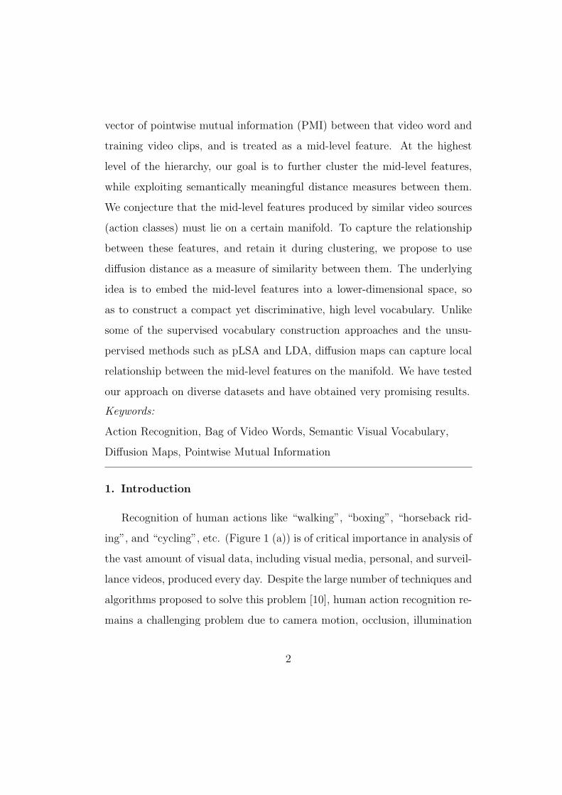
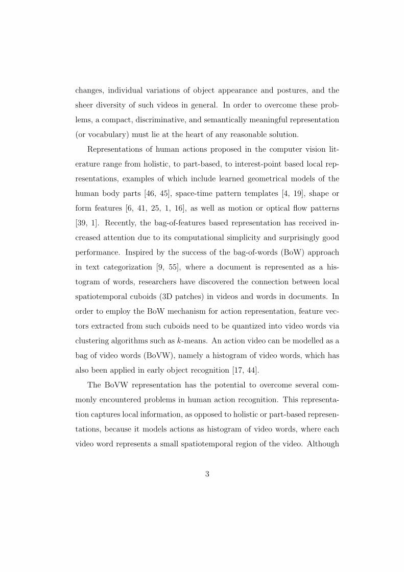
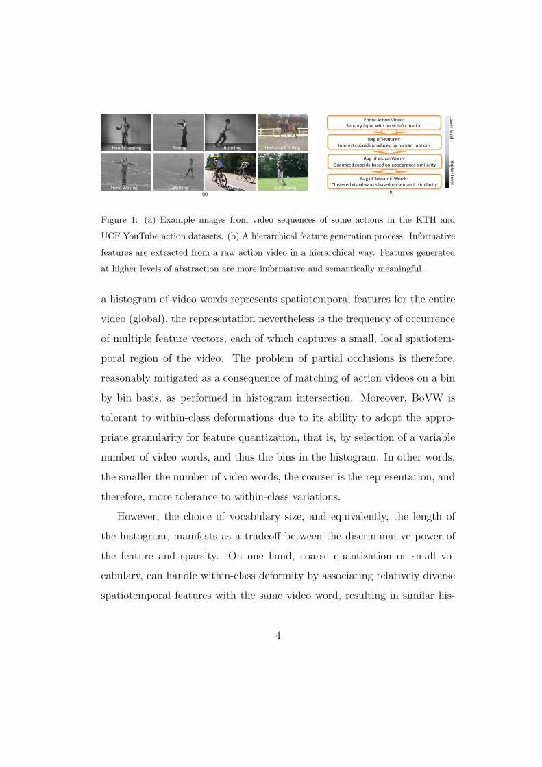
Figure 1: (a) Example images from video sequences of some actions in the KTH and

UCF YouTube action datasets. (b) A hierarchical feature generation process. Informative

features are extracted from a raw action video in a hierarchical way. Features generated

at higher levels of abstraction are more informative and semantically meaningful.

a histogram of video words represents spatiotemporal features for the entire

video (global), the representation nevertheless is the frequency of occurrence

of multiple feature vectors, each of which captures a small, local spatiotem-

poral region of the video. The problem of partial occlusions is therefore,

reasonably mitigated as a consequence of matching of action videos on a bin

by bin basis, as performed in histogram intersection. Moreover, BoVW is

tolerant to within-class deformations due to its ability to adopt the appro-

priate granularity for feature quantization, that is, by selection of a variable

number of video words, and thus the bins in the histogram. In other words,

the smaller the number of video words, the coarser is the representation, and

therefore, more tolerance to within-class variations.

However, the choice of vocabulary size, and equivalently, the length of

the histogram, manifests as a tradeoff between the discriminative power of

the feature and sparsity. On one hand, coarse quantization or small vo-

cabulary, can handle within-class deformity by associating relatively diverse

spatiotemporal features with the same video word, resulting in similar his-

4

tograms representing the video clips. On the other hand, larger vocabulary

size (i.e., fine quantization) makes the representation high dimensional, and

often sparse, which may cause the model to be noise-prone, and inefficient

for weak classifiers, like the KNN classifier. Therefore, the question, “what

is the optimal video vocabulary?” is a common concern when employing the

BoVW framework, and the proposed work attempts to answer that.

Another factor that significantly effects performance of the BoVWmethod,

is the space in which features at various levels are compared. This problem

can be broken down into the choice of distance measures, clustering methods,

and dimensionality reduction techniques. For example, the local spatiotem-

poral features computed around an interest point (e.g., cuboid feature [13])

are high dimensional vectors when linearized, and their dimensionality is of-

ten reduced using PCA. Similarly, the video words are usually obtained by

performing K-means clustering on these local spatiotemporal features, often

using the Euclidean distance between dimensionality-reduced feature vec-

tors. In other words, the video words are generated based on the similarity

of appearance, while ignoring their co-occurrence statistics, and their rela-

tionship to the videos. An important direction for improvement therefore, is

to exploit the semantic similarity between the features at different levels, to

obtain a higher level, more abstract representation. This can be achieved by

a hierarchical clustering approach, where the distance between video words

reflects their co-occurrence in the training videos.

We propose a novel framework to construct a compact yet discriminative

visual vocabulary from the lower-level BoVW representation. As shown in

Figure 1(b), the process of generating such vocabulary is to extract multi-

5

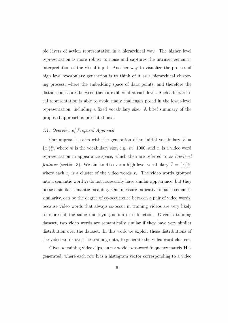
ple layers of action representation in a hierarchical way. The higher level

representation is more robust to noise and captures the intrinsic semantic

interpretation of the visual input. Another way to visualize the process of

high level vocabulary generation is to think of it as a hierarchical cluster-

ing process, where the embedding space of data points, and therefore the

distance measures between them are different at each level. Such a hierarchi-

cal representation is able to avoid many challenges posed in the lower-level

representation, including a fixed vocabulary size. A brief summary of the

proposed approach is presented next.

1.1. Overview of Proposed Approach

Our approach starts with the generation of an initial vocabulary V =

{xi}m1 , where m is the vocabulary size, e.g., m=1000, and xi is a video word

representation in appearance space, which then are referred to as low-level

features (section 3). We aim to discover a high level vocabulary V = {zj}k1,

where each zj is a cluster of the video words xi. The video words grouped

into a semantic word zj do not necessarily have similar appearance, but they

possess similar semantic meaning. One measure indicative of such semantic

similarity, can be the degree of co-occurrence between a pair of video words,

because video words that always co-occur in training videos are very likely

to represent the same underlying action or sub-action. Given a training

dataset, two video words are semantically similar if they have very similar

distribution over the dataset. In this work we exploit these distributions of

the video words over the training data, to generate the video-word clusters.

Given n training video clips, an n×m video-to-word frequency matrixH is

generated, where each row h is a histogram vector corresponding to a video

6

and each column corresponds to a video word, the video words similarity

can be estimated by the distance between the column vectors of H. These

columns are representative of how video words are distributed across the

video clips. However, the video word frequency per video may be noisy,

and sensitive to the choice of the number of video words, m. Therefore, we

convert each video-word’s frequency of occurrence to the Pointwise Mutual

Information (PMI) [56, 47], which is used to measure the degree of association

between a pair of discrete instances, and has been widely used to measure

word-to-word similarity in text analysis [57]. The PMI between the video and

the video word is simply a different representation of a video word, which

approximates the distribution of a video word over the training dataset. We

refer to the PMI representation of video words as the mid-level features.

By means of PMI, each video word then corresponds to an n-dimensional

PMI vector (where n is the number of training videos), rather than a d-

dimensional appearance vector. In order to approximate precisely the real

distribution of video words over the videos, we usually select hundreds or

thousands of training videos. We observe however, that these high dimen-

sional vectors often represent redundant information, since each action class

is likely to have multiple examples. Moreover, the redundancy increases with

the increase in number of training videos even when the number of action

classes is constant. In other words, there is obviously a high correlation be-

tween the particular dimensions of these features that correspond to videos

of the same class. The PMI feature vectors can therefore be characterized by

far fewer parameters (dimensions) than n. We conjecture that the features

produced by similar sources (i.e., videos of the same class) are likely to lie on a

7

dynamic feature manifold. Therefore, unlike our previous works [23, 22, 24],

in which we directly cluster the video words located in Rn space, we embed

each mid-level feature into a low-dimensional space that can make the fea-

tures more discriminative, while preserving the semantic “structure” of the

data, which means similar features are placed closely in the low-dimensional

space. To this end, we propose to employ Diffusion Maps [50] as a means of

feature projection.

The diffusion process begins by organizing the video words represented

by PMI vectors as a weighted graph, where the weight of the edge between

two words (nodes) is a measure of their similarity. Once we normalize the

weight matrix and make it symmetric and positive, we can further interpret

the pairwise similarities as edge flows in a Markov random walk on the graph.

In this case, the similarity is analogous to the transition probability on the

edge. Then utilizing the spectral analysis of the Markov matrix P, we can

find the k dominant eigenvectors as the coordinates of the embedding space

and project the feature points onto that space while preserving their local

geometric relationships (distances, e.g., Euclidean). In this low dimensional

space, the Euclidean distance between two features preserves their diffusion

distance in the original high dimensional space.

Notice that when interpreted as a Markov matrix, the edge weights of

the graph correspond to the probability of jumping (in the Markov chain)

from one node (or mid-level feature) to a neighbor, i.e., first order transi-

tion probability. In other words, this is the probability that the chain moves

from one node to another in a single time step, which is possible only if

an edge exists between the nodes, and has a reasonable weight or probabil-

8

ity. It is however entirely possible, that while such an edge does not exist,

the chain can move between these nodes via a third node, i.e., a second or-

der transition, which again indicates a high similarity between the features.

The second order transition probability can be determined from the Markov

transition matrix, P, as described later in section 4.2. It is important to

notice that in the context of the problem under consideration, the notion

of local neighborhood essentially defines a semantic or abstract scale space.

For instance, at a lower level of abstraction, i.e., assuming only lower or-

der Markov transitions, features belonging to the concepts of “baseball” and

“football” probably form distinct neighborhoods, and therefore clusters of

mid-level features. On the other hand, by allowing higher order transitions,

the same features may form a single, large cluster of mid-level features, that

can essentially be labeled as the concept of “sport”. The number of steps

allowed in the propagation of the Markov chain can be defined explicitly as

a parameter t, also known as the diffusion time, and by adjusting it, DM can

essentially perform multi-scale data analysis.

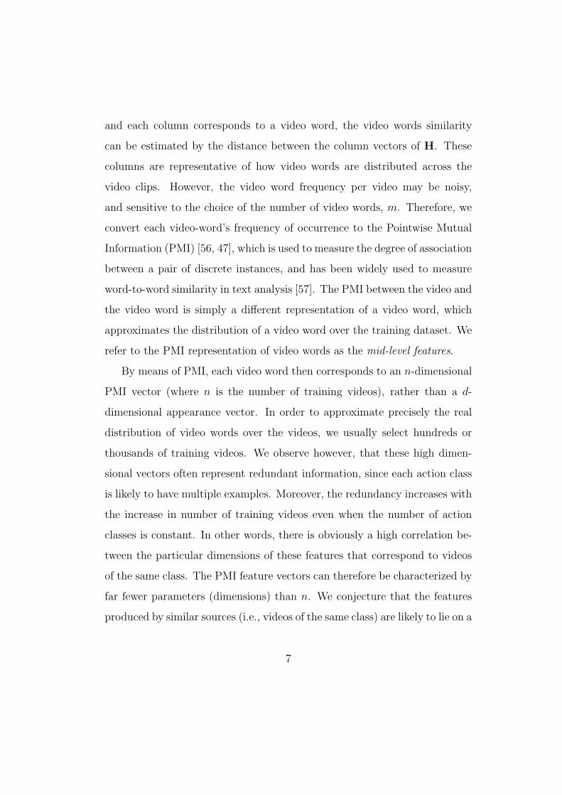
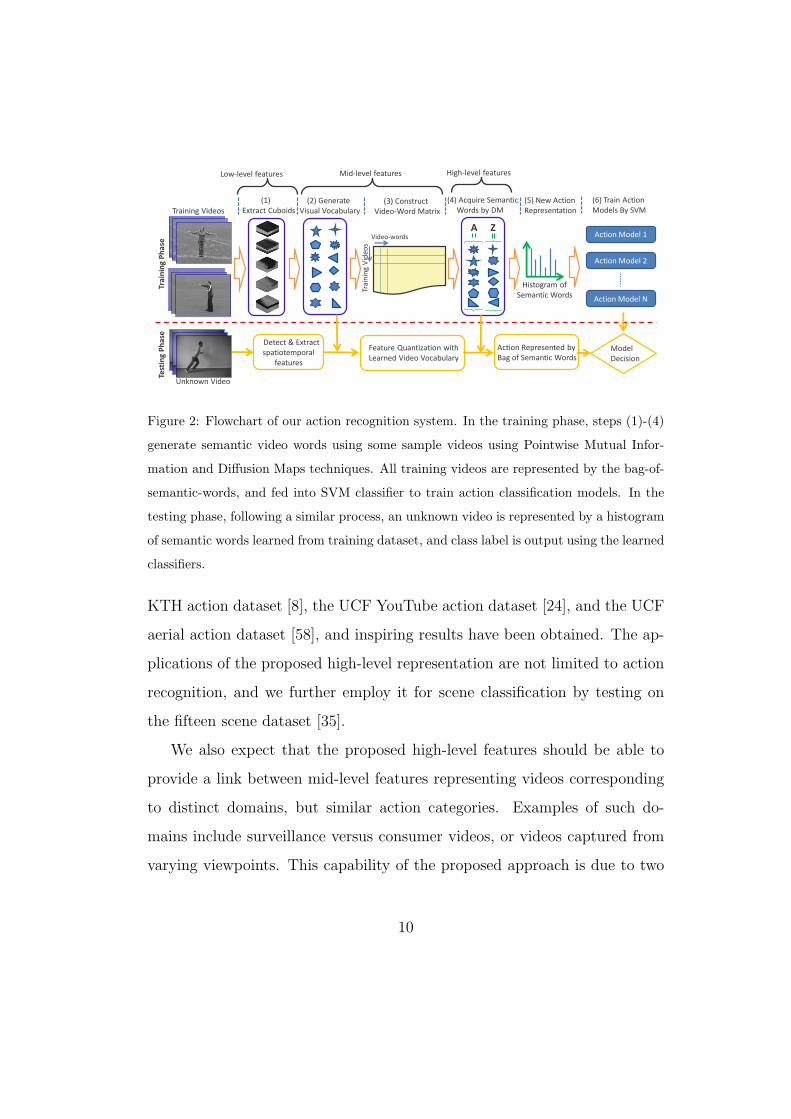
Figure 2 illustrates the flowchart of our action recognition system. In

the training phase, a semantic vocabulary is learned from an initial visual

vocabulary (constructed in step (2)). As a result, all training and testing

videos are eventually represented by histograms of the semantic words, i.e.,

high-level features, which are clusters of video-words. The action classifi-

cation models are learned by a Support Vector Machine (SVM), the input

to which are histograms of high-level features. Given an unknown video in

the testing phase, it is represented by the bag-of-semantic-word model, and

classified by a trained SVM. We have tested our proposed framework on the

9

Tra

inin

g V

ide

os

Video-words

(1)

Extract Cuboids

(2) Generate

Visual Vocabulary

(3) Construct

Video-Word Matrix

(4) Acquire Semantic

Words by DMTraining Videos

(5) New Action

Representation

(6) Train Action

Models By SVM

Action Model 1

Action Model 2

Action Model N

Histogram of

Semantic Words

Detect & Extract

spatiotemporal

features

Feature Quantization with

Learned Video Vocabulary

Action Represented by

Bag of Semantic Words

Model

Decision

Unknown Video

Tra

inin

g P

ha

seTe

stin

g P

ha

se

A Z

Low-level features Mid-level features High-level features

Figure 2: Flowchart of our action recognition system. In the training phase, steps (1)-(4)

generate semantic video words using some sample videos using Pointwise Mutual Infor-

mation and Diffusion Maps techniques. All training videos are represented by the bag-of-

semantic-words, and fed into SVM classifier to train action classification models. In the

testing phase, following a similar process, an unknown video is represented by a histogram

of semantic words learned from training dataset, and class label is output using the learned

classifiers.

KTH action dataset [8], the UCF YouTube action dataset [24], and the UCF

aerial action dataset [58], and inspiring results have been obtained. The ap-

plications of the proposed high-level representation are not limited to action

recognition, and we further employ it for scene classification by testing on

the fifteen scene dataset [35].

We also expect that the proposed high-level features should be able to

provide a link between mid-level features representing videos corresponding

to distinct domains, but similar action categories. Examples of such do-

mains include surveillance versus consumer videos, or videos captured from

varying viewpoints. This capability of the proposed approach is due to two

10

main reasons. Firstly, due to the inherent nature of the BoVW represen-

tation, features at all levels of the representational hierarchy capture only

small, local spatiotemporal regions. Assuming that training videos of the

same action have been captured from varying viewpoints, it is likely that

many such local features for the same action class will be similar in appear-

ance, and belong to the same video words. Secondly, due to the exploitation

of co-occurrence statistics in the proposed method, mid-level features that

are distributed similarly across videos are likely to cluster together. There-

fore, even if the low-level appearance features of an action appear different

from different viewpoints, they are likely to correspond to similar high-level

semantic features since they describe the same action. Based on this obser-

vation, in section 6 we explore the possibility of recognizing a novel action

from an unseen view by knowledge transfer via high-level semantic visual

representation. We test our ideas on the IXMAS multi-view action dataset

[11].

The rest of this paper is organized as follows. Section 2 reviews related

work. Section 3 describes the low-level feature extraction and action repre-

sentation. Section 4 presents the proposed framework for high-level feature

discovery. In Section 5, we compare some related manifold learning tech-

niques. Furthermore, in Section 6 we explore cross-view action recognition

using high-level features. We present our experimental results in Section 7

and conclude in Section 8.

11

2. Related Work

The problem of action recognition has inspired many unique and innova-

tive approaches. While early action recognition frameworks focused on track-

ing and analysis of tracks [32], more recently, significant progress has been

achieved by introducing novel action representations, which can be coarsely

categorized into two groups: holistic and part-based representations.

Little et al. [39] used the spatial distribution of the magnitude of the

optical flow for deriving model free features. Although it claims to have the

capacity to deal with small sized query video templates, scanning of the entire

video, for example, in a sliding window manner, is time consuming. Another

holistic approach, is to consider an action as a 3D volume and extract features

from this volume. For instance, Yilmaz et al. [4] used differential geometry

features extracted from the surfaces of spatiotemporal action volumes and

achieved good performance. This method however, requires robust tracking

to generate the 3D volumes. Parameswaran et al. [49] proposed an approach

to exploit the 2D invariance in 3D to 2D projection, and model actions using

view-invariant canonical body poses and trajectories in 2D invariance space.

It is however assumed in this method that location of body joints of the

actors are available. Bobick and Davis [2] introduced the motion-history

images, which are used to recognize several types of aerobics actions, and

Weinland et al. [11] extend this method to motion history volumes. Although

these methods are computationally efficient, they require a well segmented

foreground and background. Most holistic-based paradigms either have a

limitation on the camera motion or are computationally expensive due to

the requirement of pre-processing on the input data, such as background

12

subtraction, shape extraction, body joints extraction, object tracking and

registration.

Due to the limitation of holistic representations to solve some practical

problems, the part-based presentations have recently received more atten-

tion. Unlike the holistic-based method, this approach extracts “bag of in-

teresting parts”. Hence, it is possible to overcome certain limitations such

as background substraction and tracking. Fanti et al. [7] and Song et al.

[60] proposed a triangulated graph to model the actions. Multiple features,

such as velocity, position and appearance, were extracted from the human

body parts in a frame-by-frame manner. Spatiotemporal interest points

[20, 13, 23, 25, 24, 28] have also been widely successful. Laptev [20] computed

a saliency value for each voxel and detected the local saliency maxima based

on Harris operator. Dollar et al. [13] applied separate linear filters in the

spatial and temporal directions and detected the interest points, which have

local maxima value in both directions. An action video is then represented

by the statistical distribution of the bag of video words (BoVW).

As mention earlier however, the performance of BoVW models is sensitive

to the vocabulary size, which is partially due to the fact that video word are

not semantically meaningful. Several attempts have been made to bring

the semantic information into visual vocabularies for both object and scene

recognition and action recognition. We can categorize these attempts into

two major classes: the supervised and unsupervised approaches.

The supervised approaches use either local patch annotation [30] or im-

age/video annotation [5, 14, 31, 37, 59] to guide the construction of visual

vocabularies. Specifically, Vogel et al. [30] construct a semantic vocabulary

13

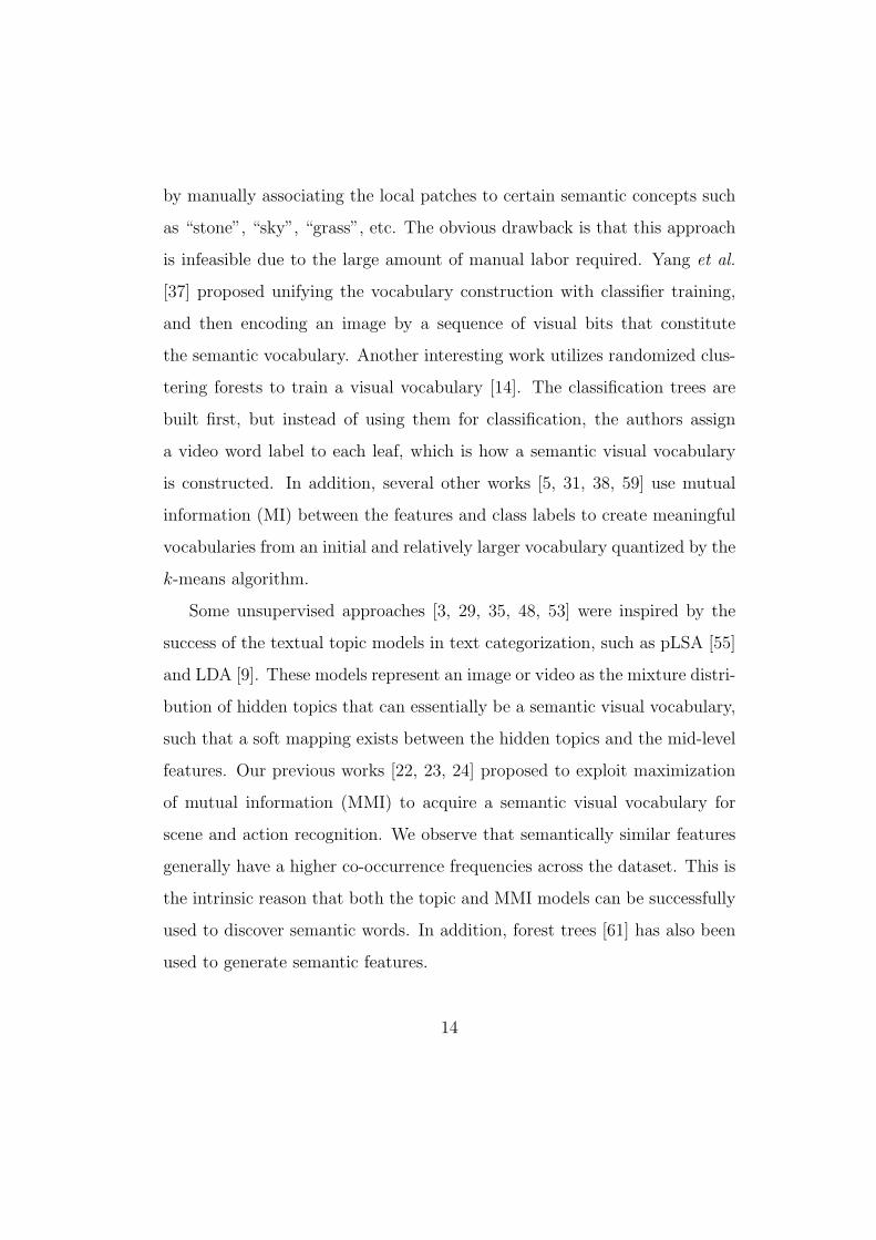
by manually associating the local patches to certain semantic concepts such

as “stone”, “sky”, “grass”, etc. The obvious drawback is that this approach

is infeasible due to the large amount of manual labor required. Yang et al.

[37] proposed unifying the vocabulary construction with classifier training,

and then encoding an image by a sequence of visual bits that constitute

the semantic vocabulary. Another interesting work utilizes randomized clus-

tering forests to train a visual vocabulary [14]. The classification trees are

built first, but instead of using them for classification, the authors assign

a video word label to each leaf, which is how a semantic visual vocabulary

is constructed. In addition, several other works [5, 31, 38, 59] use mutual

information (MI) between the features and class labels to create meaningful

vocabularies from an initial and relatively larger vocabulary quantized by the

k-means algorithm.

Some unsupervised approaches [3, 29, 35, 48, 53] were inspired by the

success of the textual topic models in text categorization, such as pLSA [55]

and LDA [9]. These models represent an image or video as the mixture distri-

bution of hidden topics that can essentially be a semantic visual vocabulary,

such that a soft mapping exists between the hidden topics and the mid-level

features. Our previous works [22, 23, 24] proposed to exploit maximization

of mutual information (MMI) to acquire a semantic visual vocabulary for

scene and action recognition. We observe that semantically similar features

generally have a higher co-occurrence frequencies across the dataset. This is

the intrinsic reason that both the topic and MMI models can be successfully

used to discover semantic words. In addition, forest trees [61] has also been

used to generate semantic features.

14

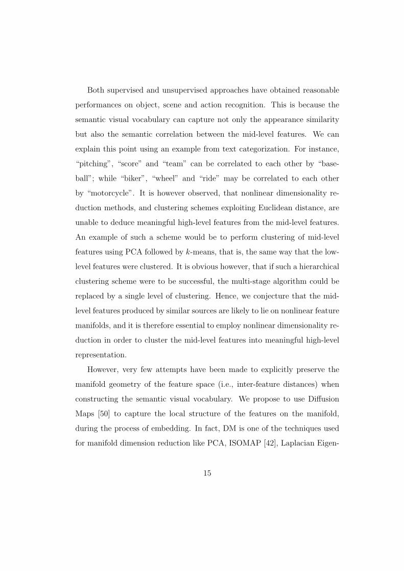
Both supervised and unsupervised approaches have obtained reasonable

performances on object, scene and action recognition. This is because the

semantic visual vocabulary can capture not only the appearance similarity

but also the semantic correlation between the mid-level features. We can

explain this point using an example from text categorization. For instance,

“pitching”, “score” and “team” can be correlated to each other by “base-

ball”; while “biker”, “wheel” and “ride” may be correlated to each other

by “motorcycle”. It is however observed, that nonlinear dimensionality re-

duction methods, and clustering schemes exploiting Euclidean distance, are

unable to deduce meaningful high-level features from the mid-level features.

An example of such a scheme would be to perform clustering of mid-level

features using PCA followed by k-means, that is, the same way that the low-

level features were clustered. It is obvious however, that if such a hierarchical

clustering scheme were to be successful, the multi-stage algorithm could be

replaced by a single level of clustering. Hence, we conjecture that the mid-

level features produced by similar sources are likely to lie on nonlinear feature

manifolds, and it is therefore essential to employ nonlinear dimensionality re-

duction in order to cluster the mid-level features into meaningful high-level

representation.

However, very few attempts have been made to explicitly preserve the

manifold geometry of the feature space (i.e., inter-feature distances) when

constructing the semantic visual vocabulary. We propose to use Diffusion

Maps [50] to capture the local structure of the features on the manifold,

during the process of embedding. In fact, DM is one of the techniques used

for manifold dimension reduction like PCA, ISOMAP [42], Laplacian Eigen-

15

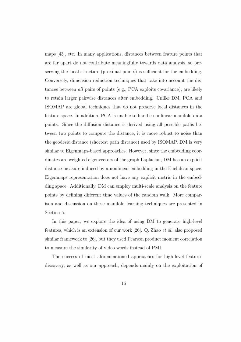
maps [43], etc. In many applications, distances between feature points that

are far apart do not contribute meaningfully towards data analysis, so pre-

serving the local structure (proximal points) is sufficient for the embedding.

Conversely, dimension reduction techniques that take into account the dis-

tances between all pairs of points (e.g., PCA exploits covariance), are likely

to retain larger pairwise distances after embedding. Unlike DM, PCA and

ISOMAP are global techniques that do not preserve local distances in the

feature space. In addition, PCA is unable to handle nonlinear manifold data

points. Since the diffusion distance is derived using all possible paths be-

tween two points to compute the distance, it is more robust to noise than

the geodesic distance (shortest path distance) used by ISOMAP. DM is very

similar to Eigenmaps-based approaches. However, since the embedding coor-

dinates are weighted eigenvectors of the graph Laplacian, DM has an explicit

distance measure induced by a nonlinear embedding in the Euclidean space.

Eigenmaps representation does not have any explicit metric in the embed-

ding space. Additionally, DM can employ multi-scale analysis on the feature

points by defining different time values of the random walk. More compar-

ison and discussion on these manifold learning techniques are presented in

Section 5.

In this paper, we explore the idea of using DM to generate high-level

features, which is an extension of our work [26]. Q. Zhao et al. also proposed

similar framework to [26], but they used Pearson product moment correlation

to measure the similarity of video words instead of PMI.

The success of most aforementioned approaches for high-level features

discovery, as well as our approach, depends mainly on the exploitation of

16

the co-occurrence information of the low-level features within the training

videos. These approaches however, usually fail to retain the spatial-temporal

relationships between the features. The compound features proposed in

[34, 18] may overcome this shortcoming. As a compound feature usually

consists of spatially or temporally proximal features, it can also capture the

co-occurrence statistics, while being limited to a small-scale neighborhood.

Therefore, [18] adopt the hierarchical grouping to acquire compound features

at various spatial or temporal co-occurrence scales (range). However, unlike

the high-level features discovered from a co-occurrence matrix, the hierar-

chical compound features may not be easily shared across distinct action

categories. As the compound features are mined from millions dense simple

features, [18] achieves better performance than our method. To ensure the

low-level features are informative, [24] use PageRank technique to mine good

low-level features before high-level features generation.

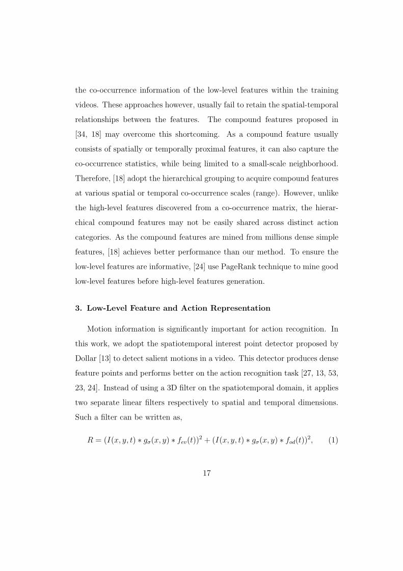
3. Low-Level Feature and Action Representation

Motion information is significantly important for action recognition. In

this work, we adopt the spatiotemporal interest point detector proposed by

Dollar [13] to detect salient motions in a video. This detector produces dense

feature points and performs better on the action recognition task [27, 13, 53,

23, 24]. Instead of using a 3D filter on the spatiotemporal domain, it applies

two separate linear filters respectively to spatial and temporal dimensions.

Such a filter can be written as,

R = (I(x, y, t) ∗ gσ(x, y) ∗ fev(t))2 + (I(x, y, t) ∗ gσ(x, y) ∗ fod(t))2, (1)

17

where gσ(x, y) is the spatial Gaussian filter with kernel σ, fev and fod are a

quadrature pair of 1D Gabor filters applied along the time dimension. They

are defined as fev(t; τ, ω) = −cos(2πtω)e−t2/τ2 and fod(t; τ, ω) = −sin(2πtω)

e−t2/τ2 , where ω = 4/τ . The parameters for two filters are set to σ=2 and

τ=1.5 in our experiments. The 3D interest points are detected at locations

where the response is locally maximum. Similar to 2D patches that are

extracted around interest points detected in an image for object recognition,

the spatiotemporal volumes around the points are extracted from the video,

which results in cuboids with a typical size of 13 × 13 × 10. Afterwards,

the gradient-based feature vectors are computed for these cuboids, and the

dimensionality is reduced to d (e.g., d=100) using PCA. As a result, a cuboid

is represented by a d-dimensional vector. Then an initial visual vocabulary is

learned from a collection of cuboids sampled from the training dataset using

k-means clustering. Each video word in the vocabulary is represented by the

centroid of the corresponding cluster in the d-dimensional appearance space.

By counting the frequency of each video word occurring in a video, we model

an action video as a histogram h of video word.

In this work, we refer the d-dimensional descriptors as low-level features,

and generally video words as mid-level features. Note that although a video

word can be represented by a d-dimensional vector, namely the centroid of

its corresponding cluster, most of the time we treat it as a symbol having

various forms in rest of this paper. The features built on video words are

referred as high-level features.

18

4. High-level Features Generation by Diffusion Maps

As discussed earlier, for reasonable action recognition, it is important

to represent an action with meaningful high-level features that are repre-

sentative of not only appearance-based similarities, but also capture the co-

occurrence statistics across action classes. However, the quantized video

words, or mid-level features, are not discriminative enough, because the ap-

pearance space alone is not semantically meaningful. The knowledge about

the labels or classes that each of the training video belongs to, is thus far

ignored. Given a training data set, we can approximate a meaningful similar-

ity measure between two video words by comparing the distribution of their

occurrences over this data. In this section, we describe the procedure of

discovering high-level video words using Pointwise Mutual Information and

Diffusion Maps techniques.

4.1. Co-occurrence Statistics

Given a training data set D = {hi}ni=1, where n is the number of train-

ing videos, hi is an m-dimensional histogram (m is the size of the initial

visual vocabulary, i.e., the number of mid-level features), we form a n ×m

video-to-word frequency matrix H = (h1,h2, ...,hn)T . If the training videos

are reasonably representative of the classes under consideration, each video

word can be approximately represented by the corresponding column zi (an

n-dimensional vector) of H, which represents the distribution of a video

word over the training videos. Therefore, the distance between two video

words in the column space of H is representative of the class based simi-

larity between them. The occurrence frequency however, is not robust to

19

noise, because as described earlier, it contains redundant information ow-

ing to multiple examples per class, and its obvious dependency on the total

number of training videos can make it highly sparse. We therefore, further

convert the co-occurrence value between a training video and a video word

to their pointwise mutual information (PMI) based representation.

The PMI between instances of two random variables Z (video words) and

Y (videos) is defined as,

pmi(z, y) = log(p(z, y)

p(z)p(y)), (2)

where p(z, y) is the joint probability. In practice, we do not know the real

joint distribution, but we observed that it can be approximated from matrix

H by normalizing the rows and columns. The marginal probabilities p(z)

and p(y) are approximated by the summation of the corresponding column

and row of the normalized H matrix respectively. Consequently, we obtain a

new video-to-word matrix H with PMI value for each entry. Each video word

is treated as a n-dimensional vector z of the column space of H instead of a

d-dimensional vector in the appearance space. This new representation then

reflects the distribution of the video words over the training data. It should

be noticed that the same video words in this work can be represented in three

different ways; (i) as d-dimensional vectors corresponding to cluster centers in

the dimension-reduced appearance space; (ii) as n-dimensional vectors z, that

are the columns of frequency matrix H; and (iii) as n-dimensional vectors z

of Pointwise Mutual Information (PMI), which are the columns of matrix H.

Although we refer to all three of these as the mid-level features, the high-

level features are subsequently computed using the third representation, i.e.,

video words represented as PMI vectors.

20

Although the Euclidean distance between two PMI vectors is somewhat

representative of their relationship, their dimensionality is determined by the

number of training videos n. Since the video words are produced by a limited

number of concepts (i.e., action classes) for the problem under consideration,

the intrinsic dimensionality of the mid-level features is much lower than n.

In other words, the dimensionality of the high-level space we wish to deduce,

is much smaller than what we observe. We conjecture that the PMI feature

vectors sharing the same source must lie on some manifold. We therefore

propose to employ non-linear dimensionality reduction using Diffusion Maps,

to discover the low-dimensional semantic space that adequately represents

such manifolds without loss of information, and in the process, make the

features more discriminative.

4.2. Feature Graph Construction

The Diffusion Maps embedding begins with the construction of a graph

of mid-level features, which we refer to as a ‘feature graph’. Graph rep-

resentation is an effective mechanism to reveal the intrinsic structure of

co-occurrence features. Given a set of mid-level features as PMI vectors

Z = {zi}mi=1, where zi ∈ Rn is a column vector of the video word matrix

H, we construct a weighted symmetric graph G(Z,W) in which each zi

corresponds to a node, and W = {wij (zi, zj)} is its weighted adjacency

matrix that is symmetric and positive. The definition of wij (zi, zj) is fully

application-driven, but it needs to represent the degree of similarity or affin-

ity of two feature points. As described earlier, we assume that the features

Z lie on a manifold. We can start with a Gaussian kernel function (or heat

conduction function), leading to a weight matrix with entries,

21

wij(zi, zj) = exp

(−∥ zi − zj ∥2

2σ

), (3)

where σ is the width (variance) of the Gaussian kernel, and ∥ zi − zj ∥ is

the Euclidean distance between the two features. When two data points are

distant in terms of the kernel width, the weight quickly decays to zero, which

means the heat can only diffuse between nearby points controlled by the

parameter σ. Larger kernel width makes the neighbors of a data point more

numerous. Hence, the graph G with weights W represents our knowledge of

the local geometric relationships between the mid-level features.

We can normalize the edge weight matrix, so that it can represent the

first order Markov transition matrix of the feature graph, and a Markov

random walk on G can then be defined. It is intuitive to notice that if two

nodes are closer (more similar), they are more likely to transmit to each

other. We can therefore treat the normalized edge weight as the transition

probability between two nodes, and consequently, matrix P = P(1) = {p(1)ij }

is constructed by normalizing matrix W such that its rows add up to 1:

p(1)ij =

wij∑k wik

. (4)

The matrix P can be considered as the transition kernel of the Markov

chain on G, which governs the evolution of the chain on the space Z. In other

words, p(1)ij defines the transition probability from node i to j in a single time

step, and P defines the entire Markov chain. P(1) reflects the first-order

neighborhood geometry of the data. We could run random walk forward in

time to capture information on larger neighborhoods by taking powers of the

matrix P. The forward probability matrix for t time steps P(t) is given by

22

[P(1)]t. The entries in P(t) represent the probability of going from i to j in t

time steps.

In such a framework, a cluster is a region in which the probability of the

Markov chain escaping this region is low. The higher the value of t, the higher

the likelihood of probabilities diffusing to further away points. The transition

matrix P(t) therefore reflects the intrinsic structure of the data set, defined

via the connectivity of the graph G, in a diffusion process and the diffusion

time t plays the role of a scale parameter in the data analysis. Generally,

smaller diffusion time means high data resolution, or finer representation,

and vice versa.

4.3. Diffusion Distance Definition

Subsequently, the diffusion distance D between two data points (mid-level

features as PMI vectors) on the feature graph can be defined by using the

random walk forward probabilities p(t)ij to relate the spectral properties of

a Markov chain (its transition matrix, eigenvalues, and eigenvectors) to the

underlying structure of the data. The underlying idea behind the diffusion

distance is to represent similarity between two data points, zi, and zj, by

comparing the likelihoods that a Markov chain transits from each of them,

to the same node, zq, by following any arbitrary path of length t. The

diffusion distance between two such data points can be written as,

[D(t)(zi, zj)]2 =

∑q∈Z

(p(t)iq − p

(t)jq )

2

φ(zq)(0), (5)

where φ(zq)(0) is the unique stationary distribution which measures the den-

sity of the features [51]. It is defined by φ(zq)(0) = dq∑

j dj, where dq is the

23

A

B

C

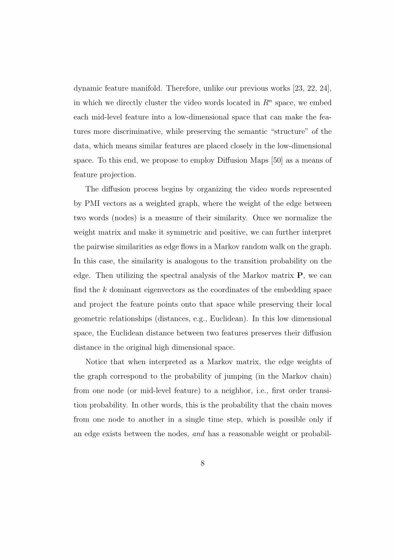
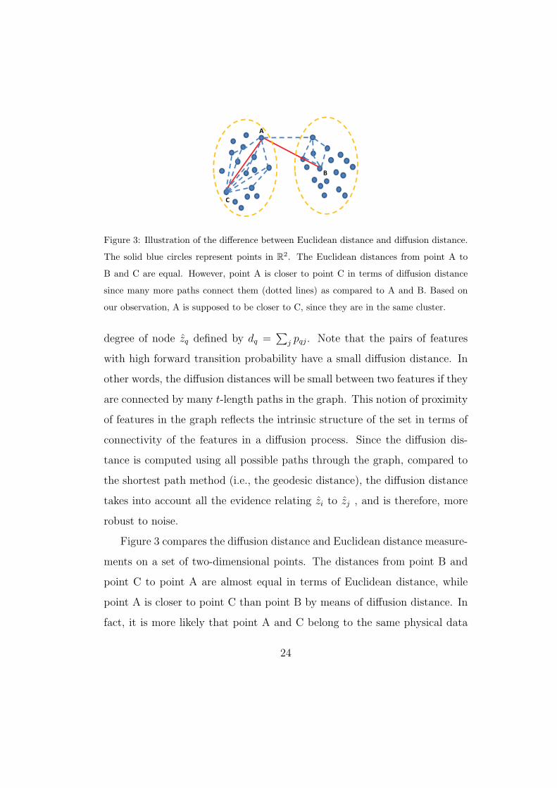
Figure 3: Illustration of the difference between Euclidean distance and diffusion distance.

The solid blue circles represent points in R2. The Euclidean distances from point A to

B and C are equal. However, point A is closer to point C in terms of diffusion distance

since many more paths connect them (dotted lines) as compared to A and B. Based on

our observation, A is supposed to be closer to C, since they are in the same cluster.

degree of node zq defined by dq =∑

j pqj. Note that the pairs of features

with high forward transition probability have a small diffusion distance. In

other words, the diffusion distances will be small between two features if they

are connected by many t-length paths in the graph. This notion of proximity

of features in the graph reflects the intrinsic structure of the set in terms of

connectivity of the features in a diffusion process. Since the diffusion dis-

tance is computed using all possible paths through the graph, compared to

the shortest path method (i.e., the geodesic distance), the diffusion distance

takes into account all the evidence relating zi to zj , and is therefore, more

robust to noise.

Figure 3 compares the diffusion distance and Euclidean distance measure-

ments on a set of two-dimensional points. The distances from point B and

point C to point A are almost equal in terms of Euclidean distance, while

point A is closer to point C than point B by means of diffusion distance. In

fact, it is more likely that point A and C belong to the same physical data

24

=

T

m

T

T

mmmmm

mkkk

m

m

zzz

zzz

zzz

zzz

P

φ

φφ

λ

λλ

ψψψ

ψψψ

ψψψψψψ

r

M

r

r

O

L

M

M

M

M

M

M

M

M

L

2

1

2

1

21

21

22212

12111

0

0

)()()(

)()()(

)()()(

)()()(

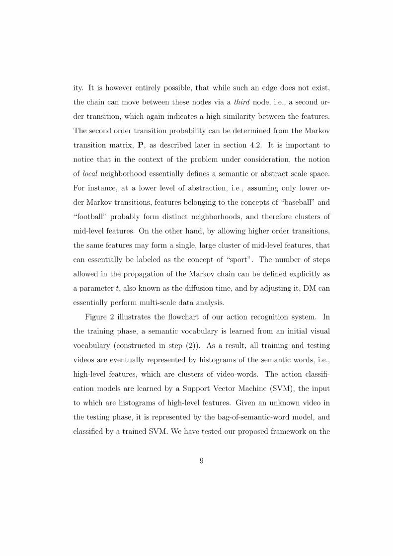
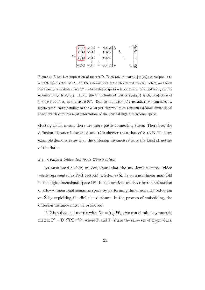
Figure 4: Eigen Decomposition of matrix P. Each row of matrix {ψi(zj)} corresponds to

a right eigenvector of P. All the eigenvectors are orthonormal to each other, and form

the basis of a feature space Rm, where the projection (coordinate) of a feature zj on the

eigenvector ψi is ψi(zj). Hence, the jth column of matrix {ψi(zj)} is the projection of

the data point zj in the space Rm. Due to the decay of eigenvalues, we can select k

eigenvectors corresponding to the k largest eigenvalues to construct a lower dimensional

space, which captures most information of the original high dimensional space.

cluster, which means there are more paths connecting them. Therefore, the

diffusion distance between A and C is shorter than that of A to B. This toy

example demonstrates that the diffusion distance reflects the local structure

of the data.

4.4. Compact Semantic Space Construction

As mentioned earlier, we conjecture that the mid-level features (video

words represented as PMI vectors), written as Z, lie on a non-linear manifold

in the high-dimensional space Rn. In this section, we describe the estimation

of a low-dimensional semantic space by performing dimensionality reduction

on Z by exploiting the diffusion distance. In the process of embedding, the

diffusion distance must be preserved.

If D is a diagonal matrix with Dii =∑

j Wij, we can obtain a symmetric

matrix P′= D1/2PD−1/2, where P and P

′share the same set of eigenvalues,

25

and we have,

P′vs = λsvs(s = 1, 2, ...,m), (6)

where λs and vs are the eigenvalue and eigenvector of P′. The left and right

eigenvectors of P are computed from vs as,

φs = vsD1/2, ψs = vsD

−1/2. (7)

Moreover, the eigenvalues and right eigenvectors of P(t) are {λts, ψs}ms=1. Us-

ing the nontrivial eigenvalues and right eigenvectors of P(t), the diffusion

distance between a pair of mid-level features can be computed (refer to [51]

for proof),

[D(t)(zi, zj)]2 =

m∑s=2

(λts)2(ψs(zi)− ψs(zj))

2, (8)

where ψs(zi) is the projection of feature zi onto eigenvector ψs. The eigenvec-

tors are orthonormal to each other, so they virtually form a semantic space

Rm. This process is illustrated in Figure 4.

Notice that not all the eigenvectors are equally important. The eigenvec-

tors corresponding to larger eigenvalues are more important as they capture

more information about the data. So we can actually use less number of

eigenvectors to span a low dimensional space. Moreover, since the first eigen-

value λ1 is equivalent to 1 [51], the corresponding eigenvector, ψ1 does not

contribute to the distance computation. As a result, the diffusion distance

can be approximated with relative precision δ using the first k nontrivial

eigenvectors and eigenvalues as,

[D(t)(zi, zj)]2 ≈

k+1∑s=2

(λts)2(ψs(zi)− ψs(zj))

2, (9)

26

where λtk+1 > δλt2. If we use the eigenvectors weighted with λ as coordinates

on the data, D(t) is virtually the Euclidean distance in the low-dimensional

space. The low-dimensional representation is therefore represented by only

k eigenvectors as,

Πt : zi 7→ {λt2ψ2(zi) λt3ψ3(zi) ... λ

tk+1ψk+1(zi)}T . (10)

The diffusion map Πt embeds the data into a Euclidean space in which

the distance is approximately the diffusion distance,

[D(t)(zi, zj)]2 w ||Πt(zi)− Πt(zj)||2. (11)

The scaling of each eigenvector by its corresponding eigenvalue leads to

a smoother mapping in the final embedding, since higher eigenvectors are

attenuated.

The mapping provides a realization of the graphG as a cloud of points in a

lower-dimensional space, where the re-scaled eigenvectors are the coordinates.

The dimensionality reduction and the weighting of the relevant eigenvectors

are dictated by both the diffusion time t of the random walk and the choice

of k, the number of eigenvectors used, which in turn depends on the spectral

fall-off of the eigenvalues. Diffusion maps embed the entire dataset in a

low-dimensional space such that the Euclidean distance is an approximation

of the diffusion distance in the high dimensional space. We summarize the

procedure of DM in Algorithm 1.

Once all video words have been embedded into the low-dimensional se-

mantic space, we apply k-means algorithm to cluster the video words into

K groups, each of which is a high-level feature. Since the k-means virtually

27

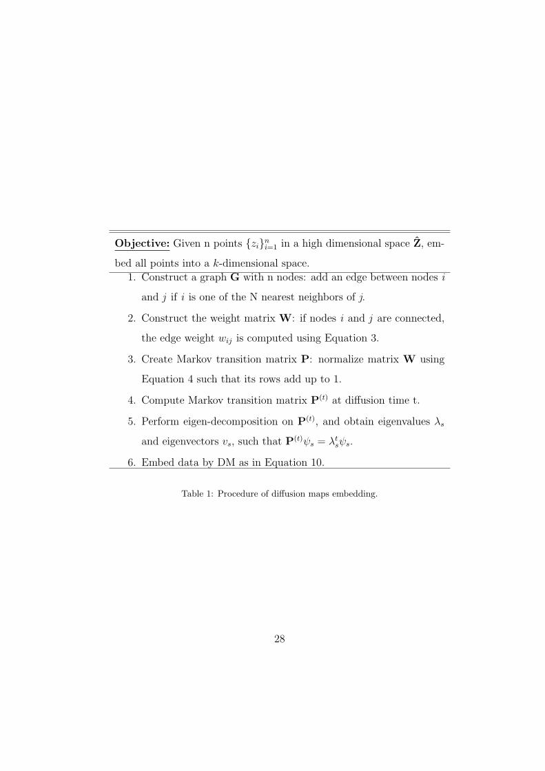
Objective: Given n points {zi}ni=1 in a high dimensional space Z, em-

bed all points into a k-dimensional space.

1. Construct a graph G with n nodes: add an edge between nodes i

and j if i is one of the N nearest neighbors of j.

2. Construct the weight matrix W: if nodes i and j are connected,

the edge weight wij is computed using Equation 3.

3. Create Markov transition matrix P: normalize matrix W using

Equation 4 such that its rows add up to 1.

4. Compute Markov transition matrix P(t) at diffusion time t.

5. Perform eigen-decomposition on P(t), and obtain eigenvalues λs

and eigenvectors vs, such that P(t)ψs = λtsψs.

6. Embed data by DM as in Equation 10.

Table 1: Procedure of diffusion maps embedding.

28

works on the semantic space, the Euclidean distance used in k-means can

reveal the semantic distance between a pair of high-level features. The clus-

tering results of k-means actually build a mapping between video words and

the semantic words (i.e., high-level features). Afterwards, we can convert the

bag-of-video-words model to the bag-of-semantic-words model.

5. Relationship to Other Embedding Methods

In order to contrast the proposed work with some of the related literature,

in this section, we provide a brief comparison of some of the more widely used

dimensionality reduction techniques in action recognition, with the Diffusion

maps framework. A more detailed comparative study can be found in [36].

PCA: PCA (principal component analysis) is a widely used technique for

linear dimensionality reduction. It is achieved by finding a few orthogonal

linear basis from the covariance matrix, which capture the largest variance

of data. Since it only tries to describe the most variance of the data by

projecting the data onto a linear basis, PCA ignores the local structure or

layout of the data and is therefore, ill-suited to manifold learning for non-

linear dimensionality reduction. Due to the fact that the projection in this

case is computed by a singular value decomposition of the covariance matrix,

PCA attempts to retain large pairwise distances instead of the small pairwise

distances, and is therefore a type of the so-called global technique. On the

other hand, since PCA deals with each dimension of the data, it does not

have the out-of-sample problem. Once new data is received, it can readily

be projected to the pre-computed linear basis. The major steps involved in

29

PCA are as following:

• Compute covariance matrix C = XX⊤ from data points arranged in a

matrix X.

• Perform Eigen decomposition of C, i.e., Cv = λv, where λ are the

eigenvalues, and v represents a matrix of eigenvectors.

• Chose the first d eigenvectors as linear basis v′.

• Project data to linear basis v′, to obtain low dimensional points, Y =

Xv′.

Notice that another useful way of comparing PCA with other spectral anal-

ysis techniques is to compute the eigenvalues and eigenvectors of the matrix,

L = X⊤X. Assume for easier intuition, that X, the matrix of data points,

is an d × n matrix, of n, d-dimensional points, where d ≫ n. Therefore, C

and L are d × d, and n × n matrices respectively. It can be shown that if

eigenvalues and eigenvectors of L are computed such that, LvL = λLvL, then

the significant eigenvectors v of C, can be related to vL as, v = XvL. It can

be noted however, that the matrix L, contains point-wise dot products for

all pairs of data points, which indeed is a reasonable measure of similarity.

In other words, L can be thought of as an edge weight matrix of a complete

graph, where the nodes are all the data points, and for every pair of nodes,

the weight is the dot product between them.

ISOMAP: Isomap uses geodesic (shortest path) distance to represent the

structure of the data. It first defines a graph G and corresponding Geodesic

30

distance weight matrix W based on K nearest neighbors of each data point,

and computes the geodesic distances between each pair. Afterwards, PCA

is employed on the pairwise geodesic distance matrix to compute the low-

dimensional representation of the data. Isomap is also a global technique

because the pairwise distance matrix captures geodesic distances between

all possible pair of points even if they are not close together. However,

since Isomap measures the geodesic distances based on the distribution of

data (by means of K nearest neighbor graph), addition of a new data point

requires new reconstruction of the graph G. Hence, Isomap suffers from

the out-of-sample problem, which also appears in Laplacian Eigenmap and

Diffusion map embeddings. Due to the fact that geodesic distance is based

on single path, small disturbance of noise data, and a resultant erroneous

neighborhood graph, can severely affect the shortest distance, and therefore,

Isomap is not particularly robust in real data scenarios. A brief overview of

the process is as follows:

• Construct a K nearest neighbor graph G of the data points X.

• Compute pairwise geodesic distance matrix, W between all pairs of

data points X, using Dijkstra’s algorithm.

• Perform PCA on pairwise geodesic distance matrix, W.

• Reduce dimensionality of data points using first d eigenvectors.

Eigenmap: Instead of considering the geodesic distance in a global manner,

Laplacian Eigenmap focuses on maintaining the local structure of the data.

31

It attempts to retain the pairwise distances between a data point and its k

nearest neighbors in the lower dimensional space. In other words, two data

points close to each other in the high dimensional space, are attempted to be

kept close after projection into the low dimensional space. Mathematically,

this is done through minimizing a cost function in a weighted manner using

Gaussian kernel function. Therefore, in the low-dimensional representation,

the distance between a data point and its first nearest neighbor contributes

more to the cost function than the distance between the data point and its

second nearest neighbor. A summary of the major steps involved in Laplacian

Eigenmap computation are:

• Construct K nearest neighbor graph G of data points, X.

• Construct weight matrix W using Gaussian kernel only for pairwise

points that are connected in G (W is sparse).

• Compute Laplacian matrix L = D−W, where D is the degree matrix

of G.

• Perform eigen decomposition, Lv = λDv.

• The eigenvectors corresponding to the smallest d eigen values form the

low dimensional space.

DM: Diffusion maps defines diffusion distance between data points by per-

forming random walk for a specific number of time steps. As opposed to

geodesic distance used in ISOMAP, the diffusion distance attempts to take

into account all possible paths on a pre-defined graph, and therefore employs

32

PCA ISOMAP Eigenmap DM

Linear yes no no no

Global yes yes no no

Parameterizes data no yes yes yes

Explicit metric no yes no yes

Pre-embedding distance - Geodesic Gaussian Diffusion

Decomposed matrix XX⊤ W D−W [P(1)](t)

Robust no no no yes

Clustering no yes no yes

Non-uniform sampling yes yes no yes

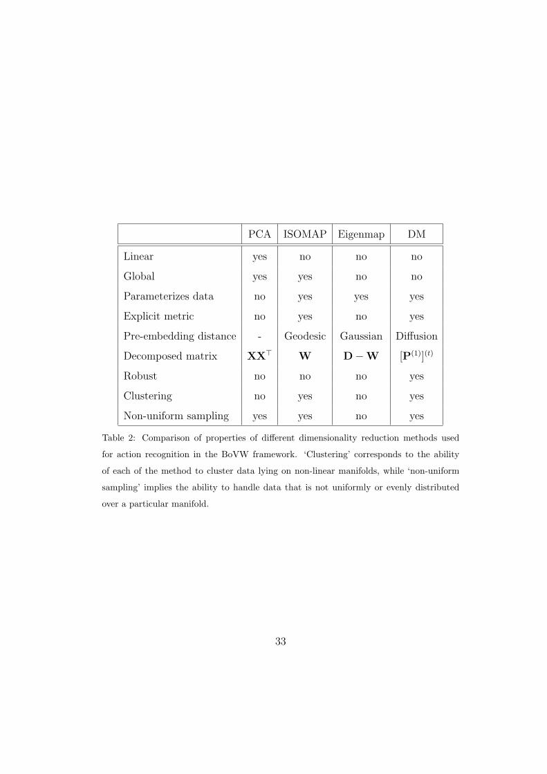
Table 2: Comparison of properties of different dimensionality reduction methods used

for action recognition in the BoVW framework. ‘Clustering’ corresponds to the ability

of each of the method to cluster data lying on non-linear manifolds, while ‘non-uniform

sampling’ implies the ability to handle data that is not uniformly or evenly distributed

over a particular manifold.

33

a much more robust measure of similarity (or distance) between data points.

Through embedding, the diffusion distance between two points in the high

dimensional space is equal to the Euclidean distance between them in the

lower dimensional space. By increasing the number of time steps t, the prob-

ability of performing random walk from one point to another increases. A

list of main steps involved are:

• Construct K nearest neighbor graph G.

• Construct weight matrix W using Gaussian kernel.

• Construct Markov transition matrix P by element-wise division of W

by diagonal degree matrix D, i.e., pij = wij/dii, where dii =∑

k wik.

• Compute tth iterate of P, i.e., the matrix P(t).

• Perform eigen decomposition of P(t), to solve P(t)v = λv.

• Eigen vectors corresponding to the largest d eigen values form the low

dimensional space.

A quantitative comparison of results obtained using these embedding

schemes is shown in section 7.2 in Figure 10, while a cursory overview of

some of their properties is listed in table 2.

6. Cross-View Action Recognition

One of the challenges frequently encountered in action recognition is the

ability to recognize actions across views. The problem arises due to the vari-

ety in appearance induced by varying camera viewpoints, as shown in Figure

34

5. In the proposed work, we attempt to use labeled actions in one view,

to train a classifier to recognize actions captured from a different view. We

observe that this task is more challenging if the actions are represented only

by mid-level features (e.g., video words) because mid-level features are based

solely on the appearance which changes drastically between views. How-

ever, regardless of the viewpoint, the video words converge to a common set

of high-level semantic features, owing to the exploitation of co-occurrence

statistics. At this level of semantic action representation, an action classi-

fication model trained on one view can be applied to test unknown videos

captured from another view.

Here, the high-level features act as a bridge between two views. This in-

tuition is illustrated in Figure 6 (a), where the semantic words are high-level

features. The semantic words, forming one common semantic vocabulary, are

constructed from two view-dependent visual vocabularies. They are treated

as the links connecting semantically similar video words of two views, which

is similar to the functionalities of bilingual words [40] and split-based de-

scriptors [15].

6.1. High-level features discovery

The discovery of semantic words starts with a training dataset Dst con-

taining pairs of unlabeled videos, where each pair has one video each, taken

from distinct viewpoints, vs and vt respectively. Those videos can be sam-

pled from whatever action categories. We then construct two sets of video

words (as Section 3 describes), forming two visual vocabularies Ws and Wt

for viewpoints vs and vt respectively. In other words, in Dst we sample videos

that are taken from view vs, and cluster their low-level features together to

35

C0

C1

C2

C3

C4

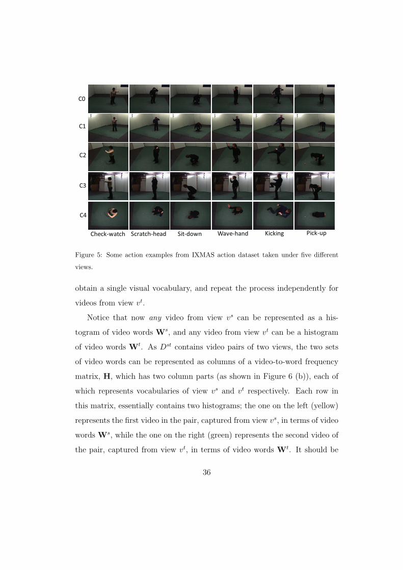
Check-watch Scratch-head Sit-down Wave-hand Kicking Pick-up

Figure 5: Some action examples from IXMAS action dataset taken under five different

views.

obtain a single visual vocabulary, and repeat the process independently for

videos from view vt.

Notice that now any video from view vs can be represented as a his-

togram of video words Ws, and any video from view vt can be a histogram

of video words Wt. As Dst contains video pairs of two views, the two sets

of video words can be represented as columns of a video-to-word frequency

matrix, H, which has two column parts (as shown in Figure 6 (b)), each of

which represents vocabularies of view vs and vt respectively. Each row in

this matrix, essentially contains two histograms; the one on the left (yellow)

represents the first video in the pair, captured from view vs, in terms of video

words Ws, while the one on the right (green) represents the second video of

the pair, captured from view vt, in terms of video words Wt. It should be

36

Visual

Vocabulary

Visual

VocabularySeman c Words

Generator by

DM

Seman c

Words

Ac on

Models

Ac on

Models

Source View Target View

(a)

Vid

eo

s

Video words

source view target view

(b)

A C

B D

Class 1, Class 2, …, Class L Class L+1, …, Class L+M

Source View

Target View

Class 1, Class 2, …, Class L Class L+1, …, Class L+M(c)

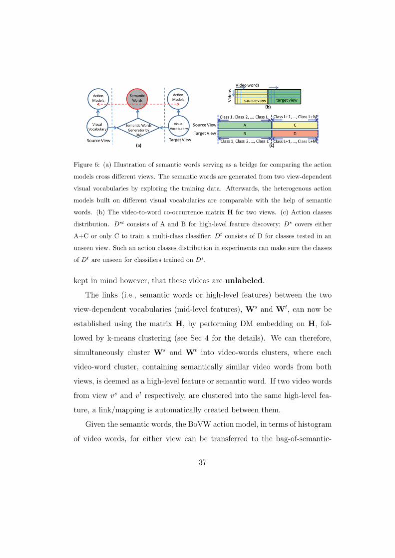
Figure 6: (a) Illustration of semantic words serving as a bridge for comparing the action

models cross different views. The semantic words are generated from two view-dependent

visual vocabularies by exploring the training data. Afterwards, the heterogenous action

models built on different visual vocabularies are comparable with the help of semantic

words. (b) The video-to-word co-occurrence matrix H for two views. (c) Action classes

distribution. Dst consists of A and B for high-level feature discovery; Ds covers either

A+C or only C to train a multi-class classifier; Dt consists of D for classes tested in an

unseen view. Such an action classes distribution in experiments can make sure the classes

of Dt are unseen for classifiers trained on Ds.

kept in mind however, that these videos are unlabeled.

The links (i.e., semantic words or high-level features) between the two

view-dependent vocabularies (mid-level features), Ws and Wt, can now be

established using the matrix H, by performing DM embedding on H, fol-

lowed by k-means clustering (see Sec 4 for the details). We can therefore,

simultaneously cluster Ws and Wt into video-words clusters, where each

video-word cluster, containing semantically similar video words from both

views, is deemed as a high-level feature or semantic word. If two video words

from view vs and vt respectively, are clustered into the same high-level fea-

ture, a link/mapping is automatically created between them.

Given the semantic words, the BoVW action model, in terms of histogram

of video words, for either view can be transferred to the bag-of-semantic-

37

words model. The transfer is very straightforward. Without loss of generality,

let h be the BoVW (histogram of video words) of a video from view vs, and

h be the corresponding transferred bag-of-semantic-word model. Then, the

value of a bin corresponding to semantic word wk is computed by, h(w) =∑zi∈wk

h(zi), where zi ∈ wk denotes all video words zi being clustered into

semantic word wk.

6.2. Recognizing actions across views

Having one set of semantic words linking two vocabularies, we are able to

conduct the cross-view action recognition task, which is formulated as follows.

Without loss of generality, let us select view vs as the source view, and view

vt as the target view. We assume Ds being a labeled action dataset captured

from the source view. Our goal is to learn a multi-class SVM classifier from

the source view dataset Ds, and then use it to classify unknown/unlabeled

videos, say Dt, captured from the target view.

In order to achieve our goal, all the training videos of Ds are first rep-

resented as the BoVW model, followed by being transferred into the bag-

of-semantic-words model. The multi-class SVM classifier is then trained on

the bag-of-semantic-words model. Given a test video from Dt, interest point

descriptors detected in it, can be categorized into video-word Wt, and the

video can therefore, be represented as a histogram of video words. Likewise,

this BoVW model of the test video is transferred into the bag-of-semantic-

words model. As a result, the multi-class classifier can be directly used to

classify the test video.

In order to make sure the testing action classes in Dt of the target view

are unseen to the multi-class classifier learned on the source view, we want

38

to ensure that the discovered semantic words do not contain action class

information of test videosDt. In our experiments we can distribute the action

classes, say action categories 1 to L+M , among the datasets as follows. The

dataset Dst, used for semantic words discovery, contains action categories 1

to L for both views vs and vt. The dataset Ds, used for training multi-class

SVM classifier on the source view, can contain action categories L + 1 to

L +M or action categories 1 to L +M on the source view only. The test

dataset Dt contains action categories L+1 to L+M on the target view. This

distribution is illustrated in Figure 6(c), where Dst covers A+B; Ds covers

C or A+C; and Dt covering D. As a result, the learned semantic words do

not convey the information of action categories L+1 to L+M in the target

view (i.e., the block D in the Figure 6(c)). Therefore, we can claim that the

action classifier learned on the source view does not see the information of

classes L + 1 to L +M in the target view. Notice that the videos of Dst

are not labeled. In practice, Dst can contain any videos depicting motion,

captured from both views.

7. Experimental Results

In this section, we first demonstrate the robustness of the diffusion dis-

tance to data noise. Then, we show the experimental results on the KTH ac-

tion dataset, the UCF YouTube action dataset, and the aerial action datasets

[12, 58]. As our approach is not limited to action recognition, we also demon-

strate that it works on the fifteen scene dataset. SVM with Histogram

Intersection kernel is chosen as the default classifier. For the KTH and

UCF YouTube action datasets, we perform the leave-one-out cross-validation

39

scheme, which means that for KTH dataset for example, 24 actors or groups

are used for training and the rest for testing.

7.1. Robustness to Noise

As aforementioned, the diffusion distance is robust to noise and small per-

turbations of the data. This results from the fact that the diffusion distance

reflects the connectivity of nodes in the graph. In other words, the distance

is computed from all the paths between two nodes s.t. all the “evidences”

are considered. Although one of the paths may be affected by the noise,

it has little weight on the computation of total diffusion distance. However,

since the geodesic distance used in ISOMAP only considers the shortest path

between two points, it is sensitive to noise, and therefore less robust to noise

than diffusion distance. In the following paragraphs, we verify this fact by

comparing the two distances in a real action data set.

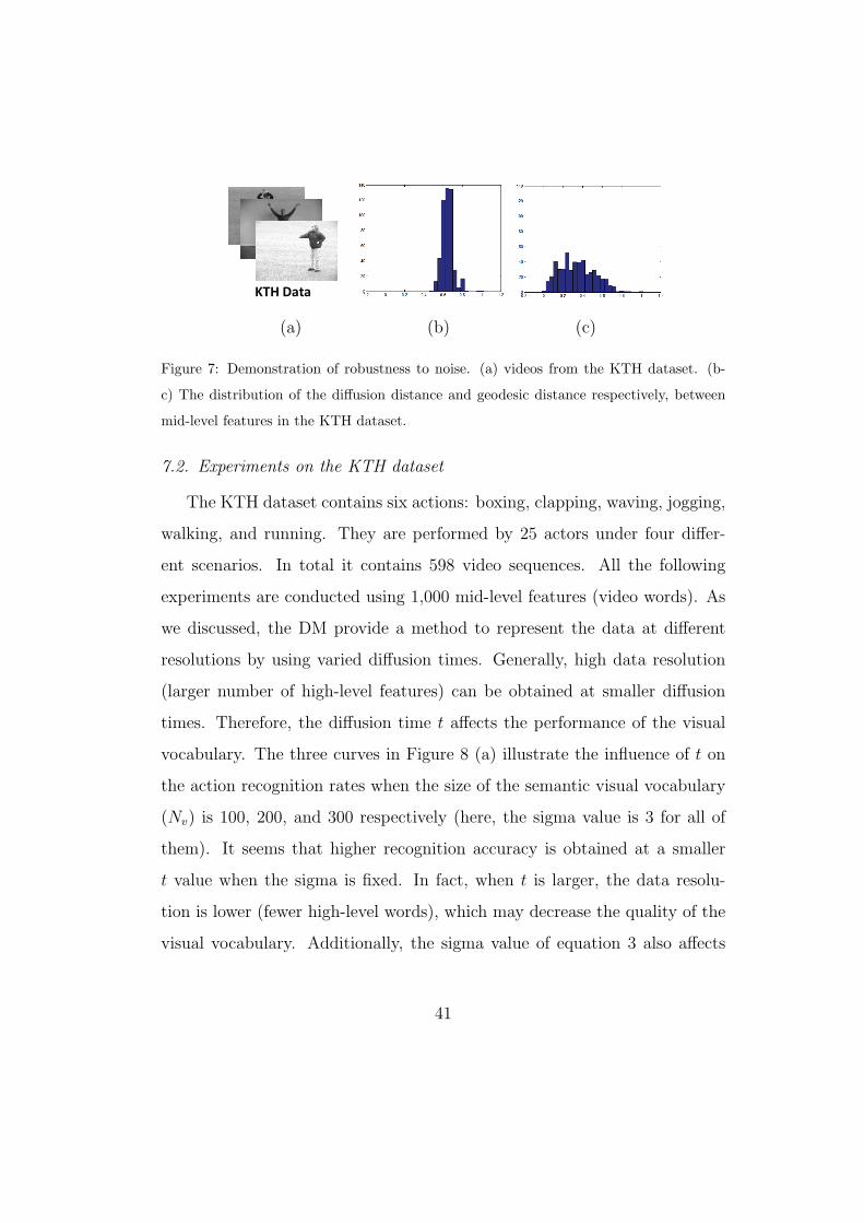
We verified the robustness of diffusion distance on the KTH dataset. We

selected two mid-level features (A and B) that have the maximum Euclidean

distance in an initial visual vocabulary with 1,000 video words (mid-level fea-

tures). Then we added Gaussian noise to the rest of features, and repeated

this procedure 500 times. For each trial, we constructed a graph as described

in section 4. The distributions of the diffusion distances and geodesic dis-

tances between mid-level features A and B are shown in Figure 7 (b) and (c).

It is obvious that diffusion distance has a much smaller standard deviation

than geodesic distance, which verifies that diffusion distance is more robust.

40

KTH Data

(a) (b) (c)

(d) (e) (f)

(a) (b) (c)

Figure 7: Demonstration of robustness to noise. (a) videos from the KTH dataset. (b-

c) The distribution of the diffusion distance and geodesic distance respectively, between

mid-level features in the KTH dataset.

7.2. Experiments on the KTH dataset

The KTH dataset contains six actions: boxing, clapping, waving, jogging,

walking, and running. They are performed by 25 actors under four differ-

ent scenarios. In total it contains 598 video sequences. All the following

experiments are conducted using 1,000 mid-level features (video words). As

we discussed, the DM provide a method to represent the data at different

resolutions by using varied diffusion times. Generally, high data resolution

(larger number of high-level features) can be obtained at smaller diffusion

times. Therefore, the diffusion time t affects the performance of the visual

vocabulary. The three curves in Figure 8 (a) illustrate the influence of t on

the action recognition rates when the size of the semantic visual vocabulary

(Nv) is 100, 200, and 300 respectively (here, the sigma value is 3 for all of

them). It seems that higher recognition accuracy is obtained at a smaller

t value when the sigma is fixed. In fact, when t is larger, the data resolu-

tion is lower (fewer high-level words), which may decrease the quality of the

visual vocabulary. Additionally, the sigma value of equation 3 also affects

41

76

78

80

82

84

86

88

90

92

1 2 3 4 5 6 7 8 9 10

Nv = 100 Nv=200 Nv=300

Diffusion Time

Av

era

ge

Acu

racc

y (

%)

72

74

76

78

80

82

84

86

88

90

92

1 2 3 4 5 6 7 8 9 10

Nv = 100 Nv = 200 Nv = 300

Sigma Value

Av

era

ge

Acu

raccy (

%)

(a) (b)

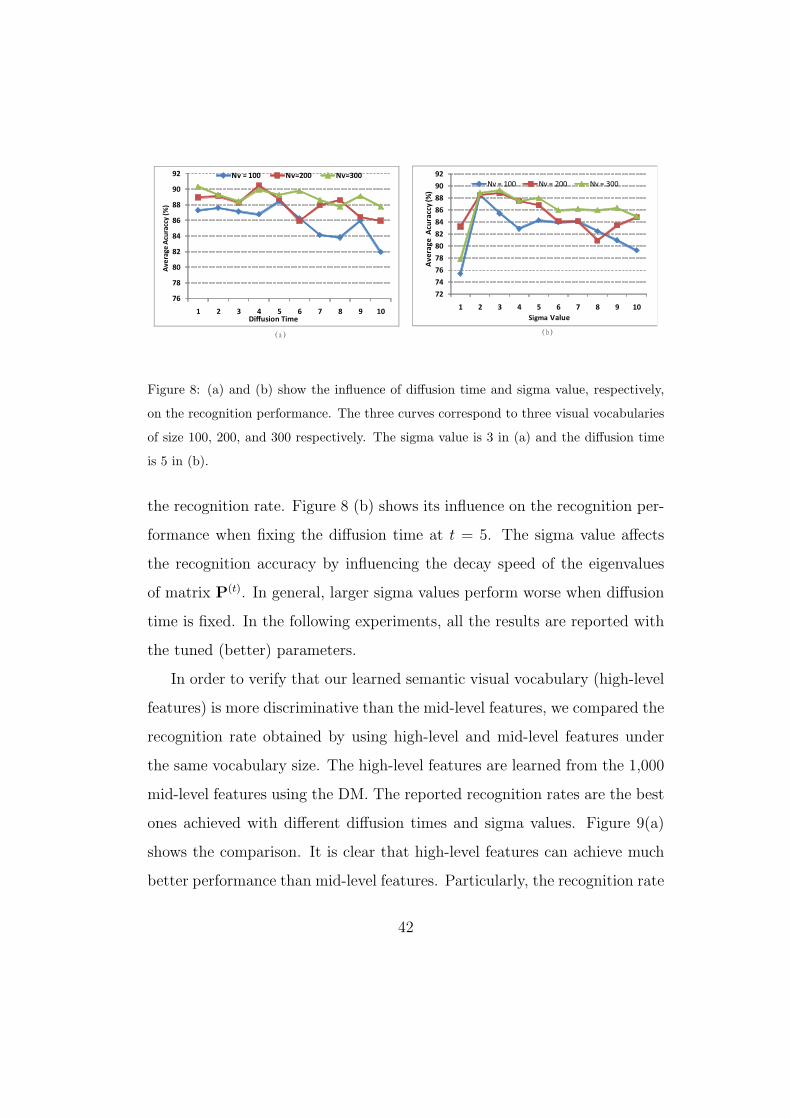
Figure 8: (a) and (b) show the influence of diffusion time and sigma value, respectively,

on the recognition performance. The three curves correspond to three visual vocabularies

of size 100, 200, and 300 respectively. The sigma value is 3 in (a) and the diffusion time

is 5 in (b).

the recognition rate. Figure 8 (b) shows its influence on the recognition per-

formance when fixing the diffusion time at t = 5. The sigma value affects

the recognition accuracy by influencing the decay speed of the eigenvalues

of matrix P(t). In general, larger sigma values perform worse when diffusion

time is fixed. In the following experiments, all the results are reported with

the tuned (better) parameters.

In order to verify that our learned semantic visual vocabulary (high-level

features) is more discriminative than the mid-level features, we compared the

recognition rate obtained by using high-level and mid-level features under

the same vocabulary size. The high-level features are learned from the 1,000

mid-level features using the DM. The reported recognition rates are the best

ones achieved with different diffusion times and sigma values. Figure 9(a)

shows the comparison. It is clear that high-level features can achieve much

better performance than mid-level features. Particularly, the recognition rate

42

65

70

75

80

85

90

95

100

25 50 100 150 200 250 300 400

midlevel features high level features

Av

era

ge

Acu

racc

y (%

)

Number of Feautres

84

85

86

87

88

89

90

91

92

93

50 100 150 200 250 300 400

DM IB

Vocabulary Size

Ave

rage

Acu

racc

y (%

)

(a) (b)

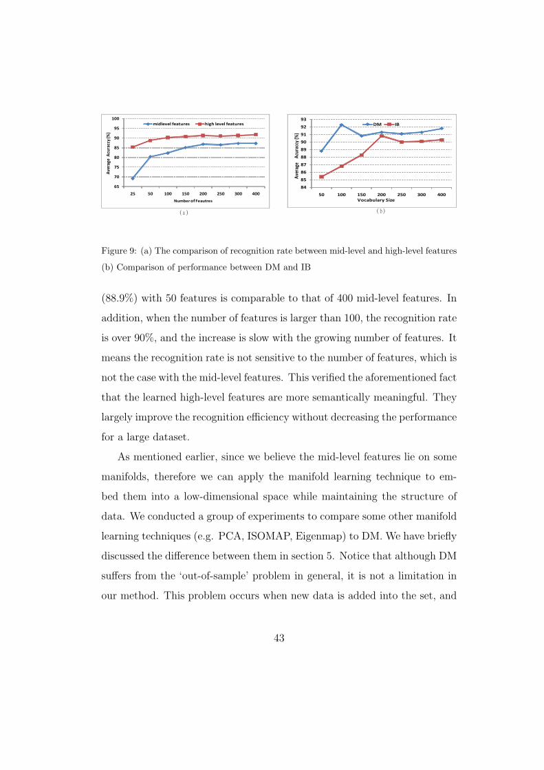
Figure 9: (a) The comparison of recognition rate between mid-level and high-level features

(b) Comparison of performance between DM and IB

(88.9%) with 50 features is comparable to that of 400 mid-level features. In

addition, when the number of features is larger than 100, the recognition rate

is over 90%, and the increase is slow with the growing number of features. It

means the recognition rate is not sensitive to the number of features, which is

not the case with the mid-level features. This verified the aforementioned fact

that the learned high-level features are more semantically meaningful. They

largely improve the recognition efficiency without decreasing the performance

for a large dataset.

As mentioned earlier, since we believe the mid-level features lie on some

manifolds, therefore we can apply the manifold learning technique to em-

bed them into a low-dimensional space while maintaining the structure of

data. We conducted a group of experiments to compare some other manifold

learning techniques (e.g. PCA, ISOMAP, Eigenmap) to DM. We have briefly

discussed the difference between them in section 5. Notice that although DM

suffers from the ‘out-of-sample’ problem in general, it is not a limitation in

our method. This problem occurs when new data is added into the set, and

43

needs to be projected into a lower-dimensional space. In our method, once

the high level vocabulary is learned, mid-level feature of new query videos

can be directly mapped to high-level features without repeating the DM em-

bedding process. In all of these experiments the mid-level features are first

embedded into a 100-dimensional space, and k-means is then employed to

obtain N clusters (high-level features). The results are shown in Figure 10(a)

(all the techniques have been tuned to have better parameters). We can see

the DM can achieve varied improvements from about 2% to 5% in terms of

recognition rate, as compared to others. Both DM and ISOMAP define an

explicit metric in the embedding space (i.e., diffusion distance and geodesic

distance respectively). These experiments further confirm that diffusion dis-

tance is more robust than geodesic distance.

Since the semantic high-level features are learned by applying k-means

clustering on the embedded mid-level features, another way to show the

effectiveness of DM embedding is to compare the recognition rate of high-

level features learned by embedded mid-level features to that of original mid-

level features without embedding (k-means is used as a clustering for both).

The results are shown in Table 3. The improvements are varied from 2.7%

to 4.0%.

Information Bottleneck (IB) can also be used to learn a semantic visual

vocabulary from the midlevel features [23, 26, 31]. Both IB and DM use

mutual information for learning. The difference is that DM uses PMI while IB

uses expectation of PMI. In addition, IB directly groups the mid-level features

without embedding them into a lower-dimensional space. The performance

comparisons between them are shown in Figure 9 (b). Although the IB can

44

75

77

79

81

83

85

87

89

91

93

95

50 100 150 200 250 300

DM Eigenmap PCA ISOMAP

Av

era

ge

A

cura

ccy

(%)

Vocabulary Size

30

35

40

45

50

55

60

65

70

75

50 100 150 200 250 300

DM EigenMap PCA ISOMAP

Ave

rage

Acu

racc

y(%

)

Vocabulary Size

(a) (b)

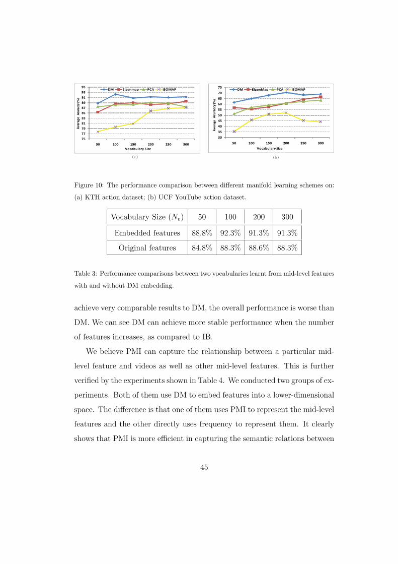
Figure 10: The performance comparison between different manifold learning schemes on:

(a) KTH action dataset; (b) UCF YouTube action dataset.

Vocabulary Size (Nv) 50 100 200 300

Embedded features 88.8% 92.3% 91.3% 91.3%

Original features 84.8% 88.3% 88.6% 88.3%

Table 3: Performance comparisons between two vocabularies learnt from mid-level features

with and without DM embedding.

achieve very comparable results to DM, the overall performance is worse than

DM. We can see DM can achieve more stable performance when the number

of features increases, as compared to IB.

We believe PMI can capture the relationship between a particular mid-

level feature and videos as well as other mid-level features. This is further

verified by the experiments shown in Table 4. We conducted two groups of ex-

periments. Both of them use DM to embed features into a lower-dimensional

space. The difference is that one of them uses PMI to represent the mid-level

features and the other directly uses frequency to represent them. It clearly

shows that PMI is more efficient in capturing the semantic relations between

45

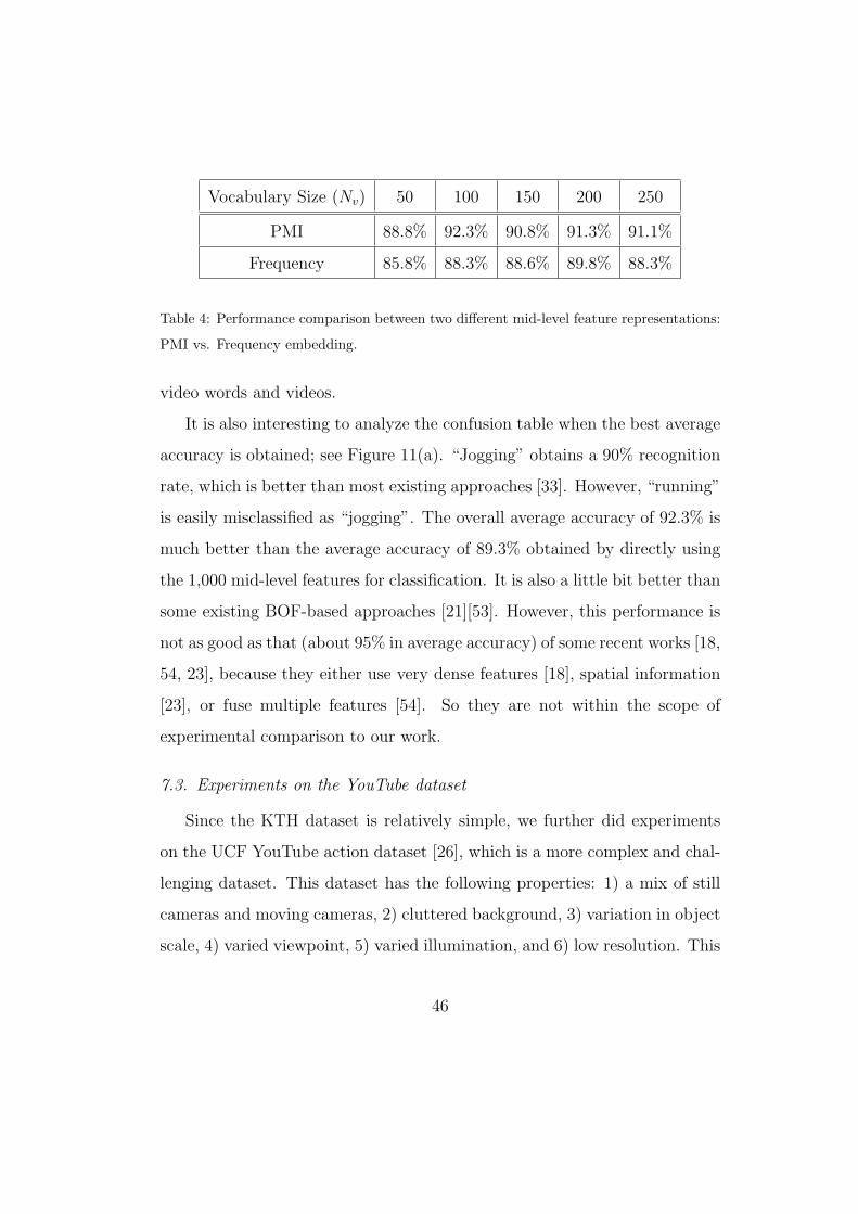
Vocabulary Size (Nv) 50 100 150 200 250

PMI 88.8% 92.3% 90.8% 91.3% 91.1%

Frequency 85.8% 88.3% 88.6% 89.8% 88.3%

Table 4: Performance comparison between two different mid-level feature representations:

PMI vs. Frequency embedding.

video words and videos.

It is also interesting to analyze the confusion table when the best average

accuracy is obtained; see Figure 11(a). “Jogging” obtains a 90% recognition

rate, which is better than most existing approaches [33]. However, “running”

is easily misclassified as “jogging”. The overall average accuracy of 92.3% is

much better than the average accuracy of 89.3% obtained by directly using

the 1,000 mid-level features for classification. It is also a little bit better than

some existing BOF-based approaches [21][53]. However, this performance is

not as good as that (about 95% in average accuracy) of some recent works [18,

54, 23], because they either use very dense features [18], spatial information

[23], or fuse multiple features [54]. So they are not within the scope of

experimental comparison to our work.

7.3. Experiments on the YouTube dataset

Since the KTH dataset is relatively simple, we further did experiments

on the UCF YouTube action dataset [26], which is a more complex and chal-

lenging dataset. This dataset has the following properties: 1) a mix of still

cameras and moving cameras, 2) cluttered background, 3) variation in object

scale, 4) varied viewpoint, 5) varied illumination, and 6) low resolution. This

46

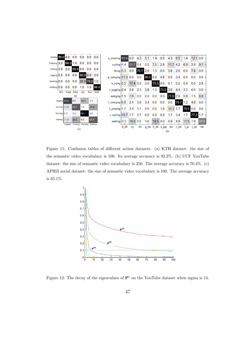
(a)

(b)

(c)

(c)

Figure 11: Confusion tables of different action datasets. (a) KTH dataset: the size of

the semantic video vocabulary is 100. Its average accuracy is 92.3%. (b) UCF YouTube

dataset: the size of semantic video vocabulary is 250. The average accuracy is 70.4%. (c)

APHill aerial dataset: the size of semantic video vocabulary is 100. The average accuracy

is 65.1%.

P

(1)

P(2)

P(4)

Figure 12: The decay of the eigenvalues of Pt on the YouTube dataset when sigma is 14.

47

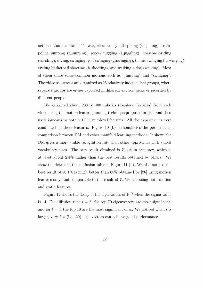
action dataset contains 11 categories: volleyball spiking (v spiking), tram-

poline jumping (t jumping), soccer juggling (s juggling), horseback-riding

(h riding), diving, swinging, golf-swinging (g swinging), tennis-swinging (t swinging),

cycling,basketball shooting (b shooting), and walking a dog (walking). Most

of them share some common motions such as “jumping” and “swinging”.

The video sequences are organized as 25 relatively independent groups, where

separate groups are either captured in different environments or recorded by

different people.

We extracted about 200 to 400 cuboids (low-level features) from each

video using the motion feature punning technique proposed in [26], and then

used k-means to obtain 1,000 mid-level features. All the experiments were

conducted on these features. Figure 10 (b) demonstrates the performance

comparison between DM and other manifold learning methods. It shows the

DM gives a more stable recognition rate than other approaches with varied

vocabulary sizes. The best result obtained is 70.4% in accuracy, which is

at least about 2.4% higher than the best results obtained by others. We

show the details in the confusion table in Figure 11 (b). We also noticed the

best result of 70.1% is much better than 65% obtained by [26] using motion

features only, and comparable to the result of 72.5% [26] using both motion

and static features.

Figure 12 shows the decay of the eigenvalues of P(t) when the sigma value

is 14. For diffusion time t = 2, the top 70 eigenvectors are most significant,

and for t = 4, the top 10 are the most significant ones. We noticed when t is

larger, very few (i.e., 20) eigenvectors can achieve good performance.

48

Digging

Running

Standing

Walking

(a) (b)

Figure 13: Examples of aerial action datasets. (a) APHill data set and, (b) UCF Aerial

data set. Each figure contains two examples each of actions, ‘digging’, ‘running’, ‘standing’,

and ‘walking’, shown as a single row. Each of the five columns correspond to five frames

of each instance.

49

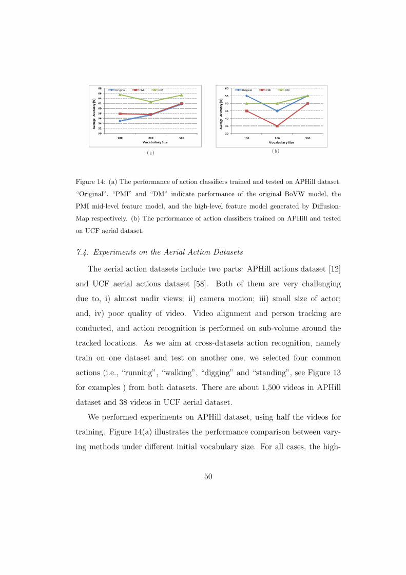
(a) (b)

50

52

54

56

58

60

62

64

66

68

100 200 500

Original PMI DM

Average

Acuraccy(%

)

Vocabulary Size

30

35

40

45

50

55

60

100 200 500

Original PMI DM

Average

Acuraccy(%

)

Vocabulary Size

Figure 14: (a) The performance of action classifiers trained and tested on APHill dataset.

“Original”, “PMI” and “DM” indicate performance of the original BoVW model, the

PMI mid-level feature model, and the high-level feature model generated by Diffusion-

Map respectively. (b) The performance of action classifiers trained on APHill and tested

on UCF aerial dataset.

7.4. Experiments on the Aerial Action Datasets

The aerial action datasets include two parts: APHill actions dataset [12]

and UCF aerial actions dataset [58]. Both of them are very challenging

due to, i) almost nadir views; ii) camera motion; iii) small size of actor;

and, iv) poor quality of video. Video alignment and person tracking are

conducted, and action recognition is performed on sub-volume around the

tracked locations. As we aim at cross-datasets action recognition, namely

train on one dataset and test on another one, we selected four common

actions (i.e., “running”, “walking”, “digging” and “standing”, see Figure 13

for examples ) from both datasets. There are about 1,500 videos in APHill

dataset and 38 videos in UCF aerial dataset.

We performed experiments on APHill dataset, using half the videos for

training. Figure 14(a) illustrates the performance comparison between vary-

ing methods under different initial vocabulary size. For all cases, the high-

50

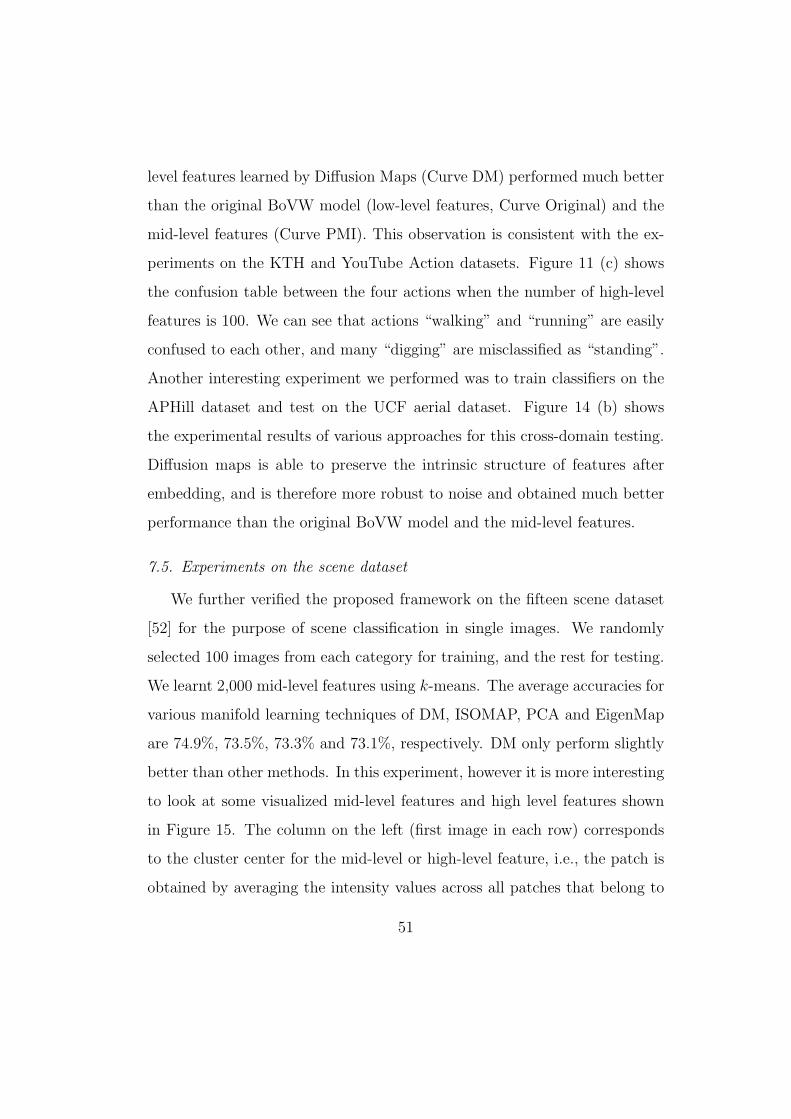
level features learned by Diffusion Maps (Curve DM) performed much better

than the original BoVW model (low-level features, Curve Original) and the

mid-level features (Curve PMI). This observation is consistent with the ex-

periments on the KTH and YouTube Action datasets. Figure 11 (c) shows

the confusion table between the four actions when the number of high-level

features is 100. We can see that actions “walking” and “running” are easily

confused to each other, and many “digging” are misclassified as “standing”.

Another interesting experiment we performed was to train classifiers on the

APHill dataset and test on the UCF aerial dataset. Figure 14 (b) shows

the experimental results of various approaches for this cross-domain testing.

Diffusion maps is able to preserve the intrinsic structure of features after

embedding, and is therefore more robust to noise and obtained much better

performance than the original BoVW model and the mid-level features.

7.5. Experiments on the scene dataset

We further verified the proposed framework on the fifteen scene dataset

[52] for the purpose of scene classification in single images. We randomly

selected 100 images from each category for training, and the rest for testing.

We learnt 2,000 mid-level features using k-means. The average accuracies for

various manifold learning techniques of DM, ISOMAP, PCA and EigenMap

are 74.9%, 73.5%, 73.3% and 73.1%, respectively. DM only perform slightly

better than other methods. In this experiment, however it is more interesting

to look at some visualized mid-level features and high level features shown

in Figure 15. The column on the left (first image in each row) corresponds

to the cluster center for the mid-level or high-level feature, i.e., the patch is

obtained by averaging the intensity values across all patches that belong to

51

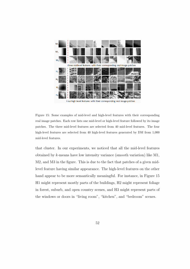
Figure 15: Some examples of mid-level and high-level features with their corresponding

real image patches. Each row lists one mid-level or high-level feature followed by its image

patches. The three mid-level features are selected from 40 mid-level features. The four

high-level features are selected from 40 high-level features generated by DM from 1,000

mid-level features.

that cluster. In our experiments, we noticed that all the mid-level features

obtained by k-means have low intensity variance (smooth variation) like M1,

M2, and M3 in the figure. This is due to the fact that patches of a given mid-

level feature having similar appearance. The high-level features on the other

hand appear to be more semantically meaningful. For instance, in Figure 15

H1 might represent mostly parts of the buildings, H2 might represent foliage

in forest, suburb, and open country scenes, and H3 might represent parts of

the windows or doors in “living room”, “kitchen”, and “bedroom” scenes.

52

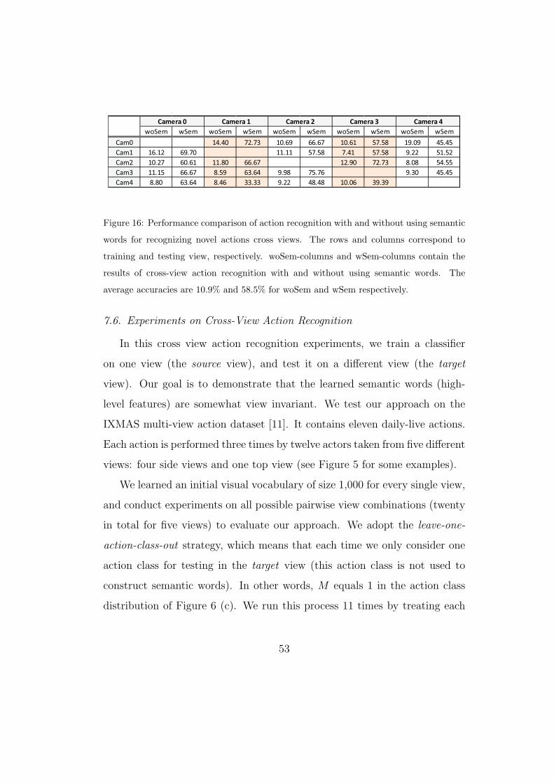
woSem wSem woSem wSem woSem wSem woSem wSem woSem wSem

Cam0 14.40 72.73 10.69 66.67 10.61 57.58 19.09 45.45

Cam1 16.12 69.70 11.11 57.58 7.41 57.58 9.22 51.52

Cam2 10.27 60.61 11.80 66.67 12.90 72.73 8.08 54.55

Cam3 11.15 66.67 8.59 63.64 9.98 75.76 9.30 45.45

Cam4 8.80 63.64 8.46 33.33 9.22 48.48 10.06 39.39

Camera 0 Camera 1 Camera 2 Camera 3 Camera 4

Figure 16: Performance comparison of action recognition with and without using semantic

words for recognizing novel actions cross views. The rows and columns correspond to

training and testing view, respectively. woSem-columns and wSem-columns contain the

results of cross-view action recognition with and without using semantic words. The

average accuracies are 10.9% and 58.5% for woSem and wSem respectively.

7.6. Experiments on Cross-View Action Recognition

In this cross view action recognition experiments, we train a classifier

on one view (the source view), and test it on a different view (the target

view). Our goal is to demonstrate that the learned semantic words (high-

level features) are somewhat view invariant. We test our approach on the

IXMAS multi-view action dataset [11]. It contains eleven daily-live actions.

Each action is performed three times by twelve actors taken from five different

views: four side views and one top view (see Figure 5 for some examples).

We learned an initial visual vocabulary of size 1,000 for every single view,

and conduct experiments on all possible pairwise view combinations (twenty

in total for five views) to evaluate our approach. We adopt the leave-one-

action-class-out strategy, which means that each time we only consider one

action class for testing in the target view (this action class is not used to

construct semantic words). In other words, M equals 1 in the action class

distribution of Figure 6 (c). We run this process 11 times by treating each

53

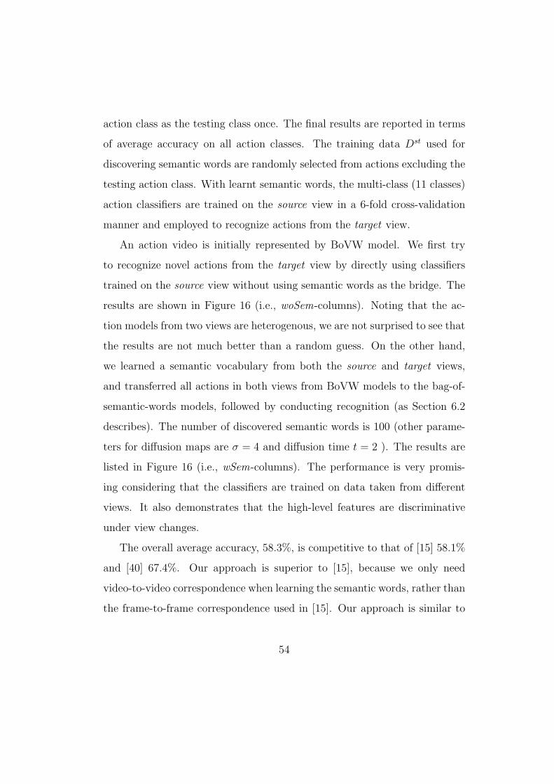
action class as the testing class once. The final results are reported in terms

of average accuracy on all action classes. The training data Dst used for

discovering semantic words are randomly selected from actions excluding the

testing action class. With learnt semantic words, the multi-class (11 classes)

action classifiers are trained on the source view in a 6-fold cross-validation

manner and employed to recognize actions from the target view.

An action video is initially represented by BoVW model. We first try

to recognize novel actions from the target view by directly using classifiers

trained on the source view without using semantic words as the bridge. The

results are shown in Figure 16 (i.e., woSem-columns). Noting that the ac-

tion models from two views are heterogenous, we are not surprised to see that

the results are not much better than a random guess. On the other hand,

we learned a semantic vocabulary from both the source and target views,

and transferred all actions in both views from BoVW models to the bag-of-

semantic-words models, followed by conducting recognition (as Section 6.2

describes). The number of discovered semantic words is 100 (other parame-

ters for diffusion maps are σ = 4 and diffusion time t = 2 ). The results are

listed in Figure 16 (i.e., wSem-columns). The performance is very promis-

ing considering that the classifiers are trained on data taken from different

views. It also demonstrates that the high-level features are discriminative

under view changes.

The overall average accuracy, 58.3%, is competitive to that of [15] 58.1%

and [40] 67.4%. Our approach is superior to [15], because we only need

video-to-video correspondence when learning the semantic words, rather than

the frame-to-frame correspondence used in [15]. Our approach is similar to

54

[40], but we do not build the bipartite graph, as [40] does, to capture the

relationship of two sets of video words. Our experiments in this section are

expected to verify a common concept that high-level features are somewhat

view invariant.

8. Conclusion

In this paper, we propose a novel approach for generic visual vocabulary

learning. We first learn the mid-level features (the initial visual vocabulary)

using k-means, then use the DM to embed the mid-level features into a low-

dimensional space while maintaining the local relationships of the features.

These embedded mid-level features are further clustered to reconstruct a se-

mantically meaningful visual vocabulary. We tested our approach on varied,

complicated datasets. The results verify that the learned semantic visual

vocabularies obtained stable performance compared to the mid-level features

learnt by k-means. In addition, we also compared DM with other manifold

learning techniques. In most cases, the DM can perform better, especially for

the action recognition datasets. Since the semantic features are reasonably

invariant to viewpoint changes, we performed experiments on recognizing

novel actions from different views. These results further verify the advan-

tages of the semantic words.

Acknowledgement: This material is based upon work supported by the

Defense Advanced Research Projects Agency (DARPA) under Contract No.

HR0011-08-C-0135.

55

References

[1] Z. Lin, Z. Jiang and L.S. Davis (2009). Recognizing actions by shape-

motion prototype trees. In Proceedings of the IEEE Conference on Com-

puter Vision and Pattern Recognition.

[2] A. Bobick and J. Davis (2001). Recognition of human movement us-

ing temporal templates. IEEE Trans. Pattern Analysis and Machine

Intelligence, 23, 3 , 257–267.

[3] A. Bosch, A. Zisserman and X. Munoz (2006). Scene classification via

plsa. In Proceedings of the European Conference on Computer Vision.

[4] A. Yilmaz and M. Shah (2005). Action sketch: A novel action repre-

setantion. In Proceddings of the IEEE Conference on Computer Vision

and Pattern Recognition.

[5] B. Fulkerson, A. Vedaldi and S. Soatto (2008). Localizing objects with

smart dictionaries. In Proceedings of European Conference on Computer

Vision.

[6] C. Carlsson and J. Sullivan. (2001). Action recognition by shape match-

ing to key frames. In Proceedings of Workshop on Models Versus Exem-

plars in Computer Vision.

[7] C. Fanti, L. Zelnik-Manor and P. Perona (2005). Hybrid models for hu-

man recognition. In Proceedings of International Conference on Com-

puter Vision and Pattern Recognition.

56

[8] C. Schuldt and I. Laptev (2004). Recognizing human actions: A lo-

cal svm approach. In Proceedings of the International Conference on

Pattern Reconition.

[9] D. Blei, A. Ng and M. Jordan (2003). Latent dirichlet allocation. Journal

of Machine Learning Research, 3, 1 , 993–1022.

[10] D. Weinland and R. Ronfardb and E. Boyer (2010). A survey of vision-

based methods for action representation, segmentation and recognition.

Computer Vision and Image Understanding , 115, 2 , 224–241.

[11] D. Weinland, R. Ronfard and E. Boyer (2006). Free viewpoint action

recognition using motion history volumes. Computer Vision and Image

Understanding , 104, 2-3 , 249–257.

[12] DARPA VIRAT APHill dataset (). Available at

http://www.viratdata.org/.

[13] Dollar, P., Rabaud, V., Cottrell, G., & Belongie, S. (2005). Behavior

recognition via sparse spatio-temporal features. In Visual Surveillance

and Performance Evaluation of Tracking and Surveillance, 2005. 2nd

Joint IEEE International Workshop on (pp. 65–72).

[14] F. Moosmann, B. Triggs and F. Jurie (2006). Fast discriminative visual

codebooks using randomized clustering forests. In Proceedings of the

Neural Information Processing Systems Conference.

[15] Farhadi, A., & Tabrizi, K. (2008). Learning to recognize activities from

the wrong view point. In Proceedings of the European Conference on

Computer Vision.

57

[16] G. Cheung, S. Baker and T. Kanade (2003). Shape-from-silhouette of ar-

ticulated objects and its use for human body kinematics estimation and

motion capture. In Proceedings of the IEEE Conference on Computer

Vision and Pattern Recognition.

[17] G. Csurka, C. R. Dance, L. Fan, J. Willamowski and C. Bray (2004).

Visual categorization with bags of keypoints. In Proceedings of the Eu-

ropean Conference on Computer Vision.

[18] Gilbert, A., Illingworth, J., & Bowden, R. (2009). Fast realistic multi-

action recognition using minded dense spatio-temporal features. In Pro-

ceedings of the IEEE International Conference on Computer Vision.

[19] Gorelick, L., Blank, M., Shechtman, E., Irani, M., & Basri, R. (2007).

Actions as space-time shapes. IEEE Transactions on Pattern Analysis

and Machine Intelligence, 29, 12 , 2247–2253.

[20] I. Laptev (2005). On space-time interst points. International Journal of

Computer Vision, 64, 2-3 , 107–123.

[21] I. Laptev, M. Marszalek, C. Schmid and B. Rozenfeld (2008). Learn-

ing realistic human actions from movies. In Proceedings of the IEEE

Conference on Computer Vision and Pattern Recognition.

[22] J. Liu and M. Shah (2007). Scene modeling using co-clustering. In

Proceedings of the IEEE International Conference on Computer Vision.

[23] J. Liu and M. Shah (2008). Learning human actions via information

maximization. In Proceedings of the IEEE Conference on Computer

Vision and Pattern Recognition.

58

[24] J. Liu, J. Luo and M. Shah (2009). Recongizing realistic actions from

videos ‘in the wild’. In Proceedings of the IEEE Conference on Computer

Vision and Pattern Recognition.

[25] J. Liu, S. Ali and M. Shah (2008). Recognizing human actions using

multiple features. In Proceedings of the IEEE Conference on Computer

Vision and Pattern Recognition.

[26] J. Liu, Y. Yang and M. Shah (2009). Learning semantic visual vocab-

ularies using diffusion distance. In Proceedings of the IEEE Conference

on Computer Vision and Pattern Recognition.

[27] J. Niebles and L. Fei-Fei (2006). Unsupervised learning of human ac-

tion categories using spatial-temporal words. In Proceedings of British

Machine Vision Conference.

[28] J. Niebles, H. Wang and L. Fei-Fei (2007). A hierarchical model of

shapes and appearance for human action classification. In Proceedings

of the IEEE Conference on Computer Vision and Pattern Recognition.

[29] J. Sivic, B. C. Russell, A. A. Efros, A. Zisserman and W. T. Freeman

(2005). Discovering objects and their location in images. In Proceedings

of the IEEE International Conference on Computer Vision.

[30] J. Vogel and B. Schiele (2004). Natural scene retrieval based on a se-

mantic modeling step. In Proceedings of the IEEE Conference on Image

and Video Retrieval .

[31] J. Winn, A. Criminisi and T. Minka (2005). Object categorization by

59

learned universal visual dictionary. In Proceedings of the International

Conference on Computer Vision.

[32] J.K. Aggarwal and Q. Cai (1997). Human motion analysis: a review. In

Proceedings of the IEEE Nonrigid and Articulated Motion Workshop.

[33] K. Mikolajczyk and H. Uemura (2008). Action recognition with motion-

appearance vocabulary forest. In Proceedings of the IEEE Conference

on Computer Vision and Pattern Recognition.

[34] Kovashka, A., & Grauman, K. (2010). Learning a hierarchy of discrim-

inative space-time neighborhood features for human action recognition.

In Proceedings of the IEEE Conference on Computer Vision and Pattern

Recognition.

[35] L. Fei-Fei and P. Perona (2005). A bayesian hierarchical model for

learning natural scene categories. In Proceedings of IEEE Conference

on Computer Vision and Pattern Recognition.

[36] L. van der Maaten, E. Postma and H. van den Herik (2008). Dimen-

sionality reduction: a comparative review. Technical Report TiCC TR

2009−005 , .

[37] L. Yang, R. Jin, R. Sukthankar and F. Jurie (2008). Unifying dis-

criminative visual codebook generation with classifier training for ob-

ject category reorganization. In Proceddings of the IEEE Conference on

Computer Vision and Pattern Recognition.

[38] Lazebnik, S., & Raginsky, M. (2008). Supervised learning of quantizer

60

codebooks by information loss minimization. IEEE transactions on pat-

tern analysis and machine intelligence, 31, 7 , 1294–1309.

[39] Little, J., & Boyd, J. (1998). Recognizing people by their gait: the shape

of motion. Videre: Journal of Computer Vision Research, 1 , 1–32.

[40] Liu, J., Shah, M., Kuipers, B., & Savarese, S. (2011). Cross-view action

recognition via view knowledge transfer. In Proceedings of the IEEE

Conference on Computer Vision and Pattern Recognition.

[41] Lv, F., & Nevatia, R. (2007). Single view human action recognition

using key pose matching and viterbi path searching. In Proceedings of

the IEEE International Conference on Computer Vision.

[42] M. Balasubramanian and E. Schwartz (2002). The isomap algorithm

and topological stability. Science, 295, 5552 , 7–13.

[43] M. Belkin and P. Niyogi (2003). Laplacian eigenmaps for dimensionality

reduction and data representation. Neural Computation, 15, 6 , 1373–

1396.

[44] Mori, G., Belongie, S., & Malik, J. (2001). Shape contexts enable effi-

cient retrieval of similar shapes. In Proceedings of the IEEE Conference

on Computer Vision and Pattern Recognition.

[45] Mori, G., & Malik, J. (2002). Estimating human body configurations us-

ing shape context matching. In Proceedings of the European Conference

on Computer Vision.

61

[46] Mori, G., Ren, X., Efros, A., & Malik, J. (2004). Recovering human body

configurations: combining segmentation and recognition. In Proceedings

of the IEEE Conference on Computer Vision and Pattern Recognition.

[47] P. Pantel and D. Lin (2002). Discovering word scenes from text. In

Proceedings of Special Interest Group on Knowledge Discovery and Data

Mining .

[48] P. Quelhas, F. Monay, J.-M Odobez, D. Gatica-Perez, T. Tuytelaars and

L. Van Gool (2005). Modeling scenes with local descriptors and latent

aspects. In Proceedings of the International Conference on Computer

Vision.

[49] Parameswaran, V., & Chellappa, R. (2006). View invariance for human

action recognition. International Journal of Computer Vision, 66, 1 ,

83–101.

[50] R.R. Coifman and S. Lafon (2006). Diffusion maps. Applied and Com-

putational harmonic Analysis , 21 , 5–23.

[51] S. Lafon and A. B. Lee (2006). Diffusion maps and coarse-graining: a

unified framework for dimensionality reduction, graph partitioning, and

data set parameterization. IEEE Transactions on Pattern Analysis and

Machine Intelligence, 28, 8 , 1393–1430.

[52] S. Lazebnik, C. Schmid and J. Ponce (2006). Beyond bags of features:

Spatial pyramid matching for recognizing natural scene categories. In

Proceedings of the IEEE Conference on Computer Vision and Pattern

Recognition.

62

[53] S. Wong, T. Kim and R. Cipolla (2007). Learning motion categories

using both semantics and structural information. In Proceedings of the

IEEE Conference on Computer Vision and Pattern Recognition.

[54] Sun, X., Chen, M., & Hauptmann, A. (2009). Action recognition via

local descriptors and holistic features. In Proceedings of the IEEE Com-

puter Society Conference on Computer Vision and Pattern Recognition

for Human Communicative Behaviour Analysis .

[55] T. Hofmann (2001). Unsupervised learning by probabilistic latent se-

mantic analysis. Machine Learning , 42, 1 , 177–196.

[56] Turney, P. (2001). Mining the web for synonyms: PMI-IR versus LSA on

TOEFL. In Proceedings of the Twelfth European Conference on Machine

Learning .

[57] Turney, P. (2002). Thumbs up or thumbs down?: semantic orientation

applied to unsupervised classification of reviews. In Proceedings of the

40th Annual Meeting on Association for Computational Linguistics .

[58] UCF Aerial dataset (). Available at

www.cs.ucf.edu/∼vision/aerial/index.html.

[59] W.H. Hsu and S. Chang (2005). Visual cue cluster construction via

information bottleneck principle and kernel density estimation. In Pro-

ceedings of the Conference on Image and Video Retrieval .

[60] Y. Song, L. Goncalves and P. Perona. (2003). Unsupervised learning of

human motion. IEEE Trans. Pattern Analysis and Machine Intelligence,

25, 25 , 814–827.

63

[61] Yu, T., Kim, T., & Cipolla, R. (2010). Real-time action recognition by

spatiotemporal semantic and structural forests. In Proceedings of the

British Machine Vision Conference.

64