E-320: Teaching Math with a Historical Perspective O. Knill, 2010-2014

Lecture 1: Mathematical roots

In the same way as one has distinguished the canons of rhetorics: memory, invention, deliv-

ery, style, and arrangement, or combined the trivium: grammar, logic and rhetorics, with the

quadrivium arithmetic, geometry, music, and astronomy, to get the seven liberal arts and

sciences, one has also tried to organize all mathematical activities.

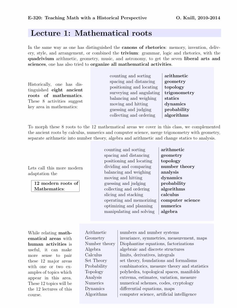
Historically, one has dis-

tinguished eight ancient

roots of mathematics.

These 8 activities suggest

key area in mathematics:

counting and sorting arithmetic

spacing and distancing geometry

positioning and locating topology

surveying and angulating trigonometry

balancing and weighing statics

moving and hitting dynamics

guessing and judging probability

collecting and ordering algorithms

To morph these 8 roots to the 12 mathematical areas we cover in this class, we complemented

the ancient roots by calculus, numerics and computer science, merge trigonometry with geometry,

separate arithmetic into number theory, algebra and arithmetic and change statics to analysis.

Lets call this more modern

adaptation the

12 modern roots of

Mathematics:

counting and sorting arithmetic

spacing and distancing geometry

positioning and locating topology

dividing and comparing number theory

balancing and weighing analysis

moving and hitting dynamics

guessing and judging probability

collecting and ordering algorithms

slicing and stacking calculus

operating and memorizing computer science

optimizing and planning numerics

manipulating and solving algebra

While relating math-

ematical areas with

human activities is

useful, it can make

more sense to pair

these 12 major areas

with one or two ex-

amples of topics which

appear in this area.

These 12 topics will be

the 12 lectures of this

course.

Arithmetic numbers and number systems

Geometry invariance, symmetries, measurement, maps

Number theory Diophantine equations, factorizations

Algebra algebraic and discrete structures

Calculus limits, derivatives, integrals

Set Theory set theory, foundations and formalisms

Probability combinatorics, measure theory and statistics

Topology polyhedra, topological spaces, manifolds

Analysis extrema, estimates, variation, measure

Numerics numerical schemes, codes, cryptology

Dynamics differential equations, maps

Algorithms computer science, artificial intelligence

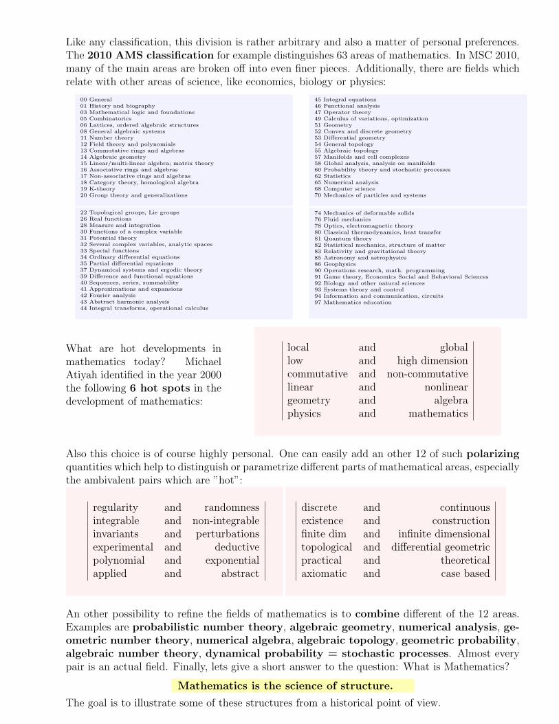
Like any classification, this division is rather arbitrary and also a matter of personal preferences.

The 2010 AMS classification for example distinguishes 63 areas of mathematics. In MSC 2010,

many of the main areas are broken off into even finer pieces. Additionally, there are fields which

relate with other areas of science, like economics, biology or physics:

00 General01 History and biography03 Mathematical logic and foundations05 Combinatorics06 Lattices, ordered algebraic structures08 General algebraic systems11 Number theory12 Field theory and polynomials13 Commutative rings and algebras14 Algebraic geometry15 Linear/multi-linear algebra; matrix theory16 Associative rings and algebras17 Non-associative rings and algebras18 Category theory, homological algebra19 K-theory20 Group theory and generalizations

45 Integral equations46 Functional analysis47 Operator theory49 Calculus of variations, optimization51 Geometry52 Convex and discrete geometry53 Differential geometry54 General topology55 Algebraic topology57 Manifolds and cell complexes58 Global analysis, analysis on manifolds60 Probability theory and stochastic processes62 Statistics65 Numerical analysis68 Computer science70 Mechanics of particles and systems

22 Topological groups, Lie groups26 Real functions28 Measure and integration30 Functions of a complex variable31 Potential theory32 Several complex variables, analytic spaces33 Special functions34 Ordinary differential equations35 Partial differential equations37 Dynamical systems and ergodic theory39 Difference and functional equations40 Sequences, series, summability41 Approximations and expansions42 Fourier analysis43 Abstract harmonic analysis44 Integral transforms, operational calculus

74 Mechanics of deformable solids76 Fluid mechanics78 Optics, electromagnetic theory80 Classical thermodynamics, heat transfer81 Quantum theory82 Statistical mechanics, structure of matter83 Relativity and gravitational theory85 Astronomy and astrophysics86 Geophysics90 Operations research, math. programming91 Game theory, Economics Social and Behavioral Sciences92 Biology and other natural sciences93 Systems theory and control94 Information and communication, circuits97 Mathematics education

What are hot developments in

mathematics today? Michael

Atiyah identified in the year 2000

the following 6 hot spots in the

development of mathematics:

local and global

low and high dimension

commutative and non-commutative

linear and nonlinear

geometry and algebra

physics and mathematics

Also this choice is of course highly personal. One can easily add an other 12 of such polarizing

quantities which help to distinguish or parametrize different parts of mathematical areas, especially

the ambivalent pairs which are ”hot”:

regularity and randomness

integrable and non-integrable

invariants and perturbations

experimental and deductive

polynomial and exponential

applied and abstract

discrete and continuous

existence and construction

finite dim and infinite dimensional

topological and differential geometric

practical and theoretical

axiomatic and case based

An other possibility to refine the fields of mathematics is to combine different of the 12 areas.

Examples are probabilistic number theory, algebraic geometry, numerical analysis, ge-

ometric number theory, numerical algebra, algebraic topology, geometric probability,

algebraic number theory, dynamical probability = stochastic processes. Almost every

pair is an actual field. Finally, lets give a short answer to the question: What is Mathematics?

Mathematics is the science of structure.

The goal is to illustrate some of these structures from a historical point of view.

E-320: Teaching Math with a Historical Perspective Oliver Knill, 2010-2014

Lecture 2: Arithmetic

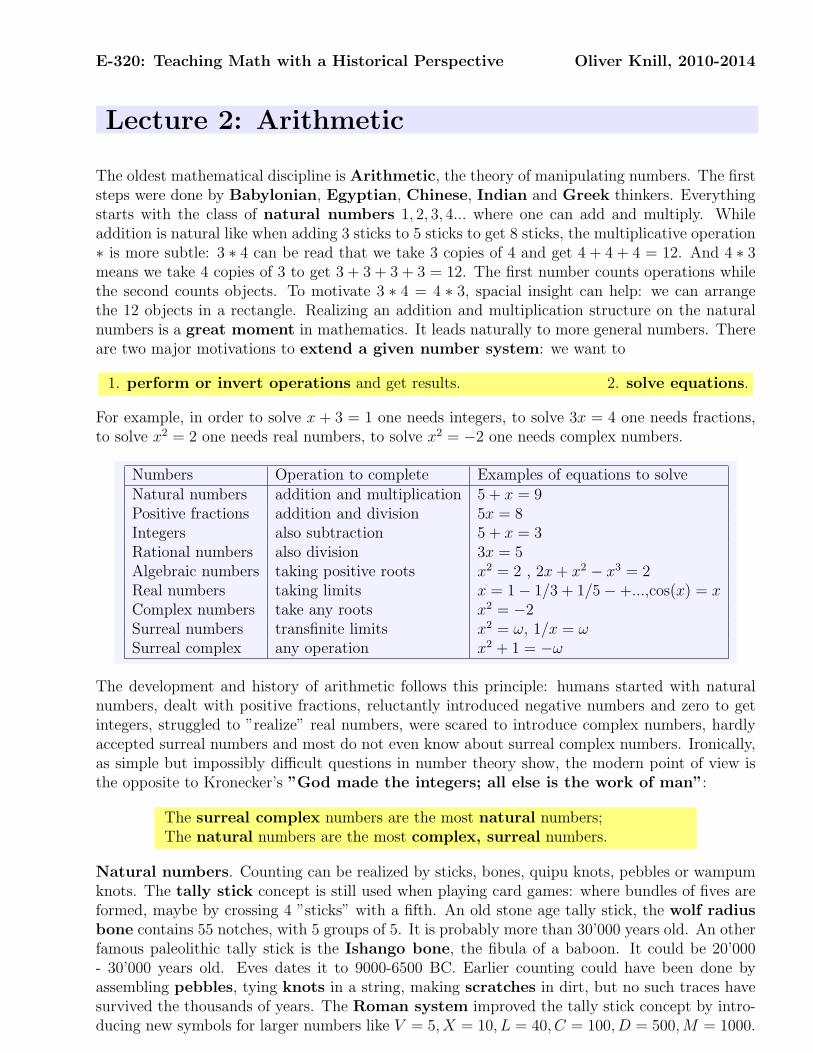
The oldest mathematical discipline is Arithmetic, the theory of manipulating numbers. The firststeps were done by Babylonian, Egyptian, Chinese, Indian and Greek thinkers. Everythingstarts with the class of natural numbers 1, 2, 3, 4... where one can add and multiply. Whileaddition is natural like when adding 3 sticks to 5 sticks to get 8 sticks, the multiplicative operation∗ is more subtle: 3 ∗ 4 can be read that we take 3 copies of 4 and get 4 + 4 + 4 = 12. And 4 ∗ 3means we take 4 copies of 3 to get 3 + 3 + 3 + 3 = 12. The first number counts operations whilethe second counts objects. To motivate 3 ∗ 4 = 4 ∗ 3, spacial insight can help: we can arrangethe 12 objects in a rectangle. Realizing an addition and multiplication structure on the naturalnumbers is a great moment in mathematics. It leads naturally to more general numbers. Thereare two major motivations to extend a given number system: we want to

1. perform or invert operations and get results. 2. solve equations.

For example, in order to solve x + 3 = 1 one needs integers, to solve 3x = 4 one needs fractions,to solve x2 = 2 one needs real numbers, to solve x2 = −2 one needs complex numbers.

Numbers Operation to complete Examples of equations to solveNatural numbers addition and multiplication 5 + x = 9Positive fractions addition and division 5x = 8Integers also subtraction 5 + x = 3Rational numbers also division 3x = 5Algebraic numbers taking positive roots x2 = 2 , 2x+ x2 − x3 = 2Real numbers taking limits x = 1− 1/3 + 1/5−+...,cos(x) = xComplex numbers take any roots x2 = −2Surreal numbers transfinite limits x2 = ω, 1/x = ωSurreal complex any operation x2 + 1 = −ω

The development and history of arithmetic follows this principle: humans started with naturalnumbers, dealt with positive fractions, reluctantly introduced negative numbers and zero to getintegers, struggled to ”realize” real numbers, were scared to introduce complex numbers, hardlyaccepted surreal numbers and most do not even know about surreal complex numbers. Ironically,as simple but impossibly difficult questions in number theory show, the modern point of view isthe opposite to Kronecker’s ”God made the integers; all else is the work of man”:

The surreal complex numbers are the most natural numbers;The natural numbers are the most complex, surreal numbers.

Natural numbers. Counting can be realized by sticks, bones, quipu knots, pebbles or wampumknots. The tally stick concept is still used when playing card games: where bundles of fives areformed, maybe by crossing 4 ”sticks” with a fifth. An old stone age tally stick, the wolf radius

bone contains 55 notches, with 5 groups of 5. It is probably more than 30’000 years old. An otherfamous paleolithic tally stick is the Ishango bone, the fibula of a baboon. It could be 20’000- 30’000 years old. Eves dates it to 9000-6500 BC. Earlier counting could have been done byassembling pebbles, tying knots in a string, making scratches in dirt, but no such traces havesurvived the thousands of years. The Roman system improved the tally stick concept by intro-ducing new symbols for larger numbers like V = 5, X = 10, L = 40, C = 100, D = 500,M = 1000.

in order to avoid bundling too many single sticks. The system is unfit for computations as simplecalculations V III + V II = XV show. Clay tablets, some as early as 2000 BC and others from600 - 300 BC are known. They feature Akkadian arithmetic using the base 60. The hexadec-imal system with base 60 is convenient becuase of many factors. It survived: we use 60 minutesper hour. The Egyptians used the base 10. The most important source on Egyptian mathe-matics is the Rhind Papyrus of 1650 BC. Hieratic numerals were used to write on papyrus from2500 BC on. Egyptian numerals are hieroglyphics. They were found in carvings on tombs andmonuments and are 5000 years old. The modern way to write numbers like the number 2010 is theHindu-Arab system which diffused to the West only during the late Middle ages. It replacedthe more primitive Roman system. Greek arithmetic used a primitive number system with noplace values: 9 Greek letters for 1, 2, . . . 9, nine for 10, 20, . . . , 90 and nine for 100, 200, . . . , 900.

Integers. Indian Mathematics morphed the place-value system into a modern method ofwriting numbers. Hindu astronomers used words to represent digits, but the numbers would bewritten in the opposite order. Sometimes after 500, the Hindus changed to a digital notationwhich included the symbol 0. Negative numbers were introduced around 100 BC in the Chinese

text ”Nine Chapters on the Mathematica art”. Also the Bakshali manuscript, written around300 AD subtracts numbers carried out additions with negative numbers, where + was used toindicate a negative sign. In Europe, negative numbers were avoided until the 15’th century.

Fractions: Babylonians could handle fractions. The Egyptians also used fractions, butwrote every fraction a as a sum of fractions with unit numerator and distinct denominators,like 4/5 = 1/2 + 1/4 + 1/20 or 5/6 = 1/2 + 1/3. Because of this cumbersome computation,Egyptian mathematics failed to progress beyond a primitive stage. The modern decimal fractionsused nowadays for numerical calculations were adopted in Europe only in 1595.

Real numbers: It was the Greeks who realized first that some naturally occurring lengths areirrational: the insight that the diagonal of the square is not a rational number produced a cri-sis. Only much later, it became clear that ”most” numbers are not rational. Georg Cantor

realized first that the cardinality of all real numbers is much larger than the cardinality of theintegers: while one can enumerate all integers and rational numbers, one can not enumerate thereal numbers. One consequence is that most real numbers are transcendental: most numbersdo not occur as solutions of polynomial equations with integer coefficients. The number π is anexample. The concept of real numbers is closely related to the concept of limit. Sums like1 + 1/4 + 1/9 + 1/16 + 1/25 + ... approach real numbers which are not rational any more.

Complex numbers: Not every polynomial equation has a real solution. To solve x2 = −1 forexample, we need new numbers. One idea is to use pairs of numbers (a, b) where (a, 0) = a arethe usual numbers and extend addition and multiplication (a, b) + (c, d) = (a + c, b + d) and(a, b) · (c, d) = (ac − bd, ad + bc). With this multiplication, the number (0, 1) has the propertythat (0, 1) · (0, 1) = (−1, 0) = −1. It is more convenient to write a + ib where i = (0, 1) satisfiesi2 = −1. One can now use the common rules of addition and multiplication.

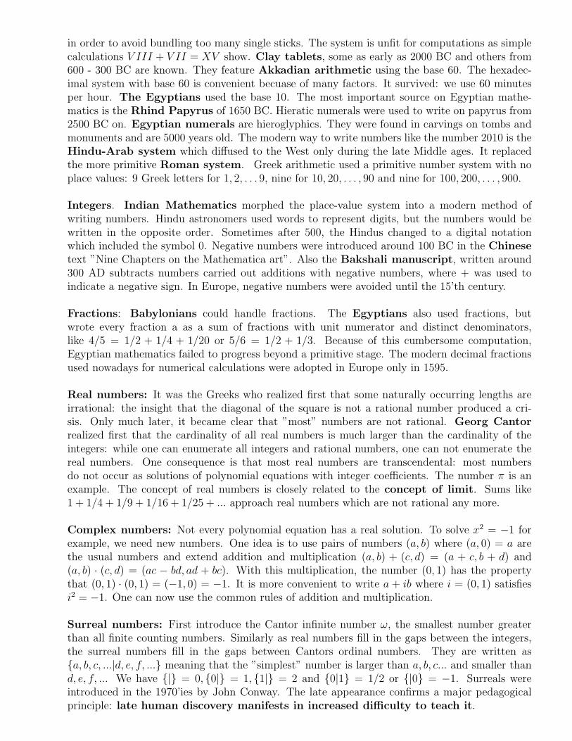
Surreal numbers: First introduce the Cantor infinite number ω, the smallest number greaterthan all finite counting numbers. Similarly as real numbers fill in the gaps between the integers,the surreal numbers fill in the gaps between Cantors ordinal numbers. They are written asa, b, c, ...|d, e, f, ... meaning that the ”simplest” number is larger than a, b, c... and smaller thand, e, f, ... We have | = 0, 0| = 1, 1| = 2 and 0|1 = 1/2 or |0 = −1. Surreals wereintroduced in the 1970’ies by John Conway. The late appearance confirms a major pedagogicalprinciple: late human discovery manifests in increased difficulty to teach it.

E-320: Teaching Math with a Historical Perspective Oliver Knill, 2010-2014

Lecture 3: Geometry

Geometry is the science of shape, size and symmetry. While arithmetic dealt with numericalstructures, geometry deals with metric structures. Geometry is one of the oldest mathemati-cal disciplines and early geometry has relations with arithmetics: we have seen that that theimplementation of a commutative multiplication on the natural numbers is rooted from an inter-pretation of n×m as an area of a shape that is invariant under rotational symmetry. Numbersystems built upon the natural numbers inherit this. Identities like the Pythagorean triples

32+42 = 52 were interpreted geometrically. The right angle is the most ”symmetric” angle apartfrom 0. Symmetry manifests itself in quantities which are invariant. Invariants are one the mostcentral aspects of geometry. Felix Klein’s Erlanger program uses symmetry to classify geome-tries depending on how large the symmetries of the shapes are. In this lecture, we look at a fewresults which can all be stated in terms of invariants. In the presentation as well as the worksheetpart of this lecture, we will work us through smaller miracles like special points in triangles aswell as a couple of gems: Pythagoras, Thales,Hippocrates, Feuerbach, Pappus, Morley,Butterfly which illustrate the importance of symmetry.

Much of geometry is based on our ability to measure length, the distance between two points.A modern way to measure distance is to determine how long light needs to get from one pointto the other. This geodesic distance generalizes to curved spaces like the sphere and is also apractical way to measure distances, for example with lasers. It bypasses the problem to determinefirst the underlying nature of the space in which we do geometry. Having a distance d(A,B)between any two points A,B, we can look at the next more complicated object, which is a setA,B,C of 3 points, a triangle. Given an arbitrary triangle ABC, are there relations between the3 possible distances a = d(B,C), b = d(A,C), c = d(A,B)? If we fix the scale by c = 1, thena + b ≥ 1, a + 1 ≥ b, b + 1 ≥ a. For any pair of (a, b) in this region, there is a triangle. Afteran identification, we get an abstract space, which represent all triangles uniquely up to similarity.Mathematicians call this an example of a moduli space.

A sphere Sr(x) is the set of points which have distance r from a given point x. In the plane, the

sphere is called a circle. A natural problem is to find the circumference L = 2π of a unit circle,or the area A = π of a unit disc, the area F = 4π of a unit sphere and the volume V = 4 = π/3 ofa unit sphere. Measuring the length of segments on the circle leads to new concepts like angle orcurvature. Because the circumference of the unit circle in the plane is L = 2π, angle questionsare tied to the number π, which Archimedes already approximated by fractions.

Also volumes were among the first quantities, Mathematicians wanted to measure and com-pute. A problem on Moscow papyrus dating back to 1850 BC explains the general formulah(a2+ab+b2)/3 for a truncated pyramid with base length a, roof length b and height h. Archimedesachieved to compute the volume of the sphere: place a cone inside a cylinder. The complementof the cone inside the cylinder has on each height h the area π−πh2. The half sphere cut at heighth is a disc of radius (1 − h2) which has area π(1 − h2) too. Since the slices at each height havethe same area, the volume must be the same. The complement of the cone inside the cylinder hasvolume π − π/3 = 2π/3, half the volume of the sphere.

The first geometric playground was planimetry, the geometry in the flat two dimensional space.Highlights are Pythagoras theorem, Thales theorem, Hippocrates theorem, and Pappus

theorem. Discoveries in planimetry have been made later on: an example is the Feuerbachtheorem from the 19th century or the Sadov theorem for quadrilaterals. Greek Mathematics isclosely related to history. It starts with Thales goes over Euclid’s era at 300 BC, and endswith the threefold destruction of Alexandria 47 BC by the Romans, 392 by the Christians and640 by the Muslims. Geometry was also a place, where the axiomatic method was broughtto mathematics: theorems are proved from a few statements which are called axioms like the 5axioms of Euclid:

1. Any two distinct points A,B determines a line through A and B.2. A line segment [A,B] can be extended to a straight line containing the segment.3. A line segment [A,B] determines a circle containing B and center A.4. All right angles are congruent.5. If lines L,M intersect with a third so that inner angles add up to < π, then L,M intersect.

Euclid wondered whether the fifth postulate can be derived from the first four and called theo-rems derived from the first four the ”absolute geometry”. Only much later, with Karl-Friedrich

Gauss and Janos Bolyai and Nicolai Lobachevsky in the 19’th century in hyperbolic space

the 5’th axiom does not hold. Indeed, geometry can be generalized to non-flat, or even much moreabstract situations. Basic examples are geometry on a sphere leading to spherical geometry orgeometry on the Poincare disc, a hyperbolic space. Both of these geometries are non-Euclidean.Riemannian geometry, which is essential for general relativity theory generalizes both con-cepts to a great extent. An example is the geometry on an arbitrary surface. Curvatures of suchspaces can be computed by measuring length alone, which is how long light needs to go from onepoint to the next.

An important moment in mathematics was the merge of geometry with algebra: this giantstep is often attributed to Rene Descartes. Together with algebra, the subject leads to algebraicgeometry which can be tackled with computers: here are some examples of geometries which aredetermined from the amount of symmetry which is allowed:

Euclidean geometry Properties invariant under a group of rotations and translationsAffine geometry Properties invariant under a group of affine transformationsProjective geometry Properties invariant under a group of projective transformationsSpherical geometry Properties invariant under a group of rotationsConformal geometry Properties invariant under angle preserving transformationsHyperbolic geometry Properties invariant under a group of Mobius transformations

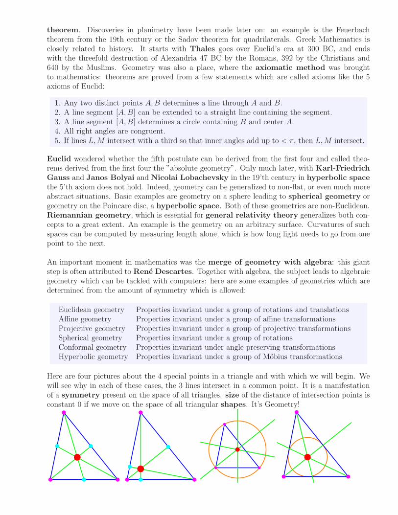
Here are four pictures about the 4 special points in a triangle and with which we will begin. Wewill see why in each of these cases, the 3 lines intersect in a common point. It is a manifestationof a symmetry present on the space of all triangles. size of the distance of intersection points isconstant 0 if we move on the space of all triangular shapes. It’s Geometry!

E-320: Teaching Math with a Historical Perspective Oliver Knill, 2014

Lecture 3: Geometry

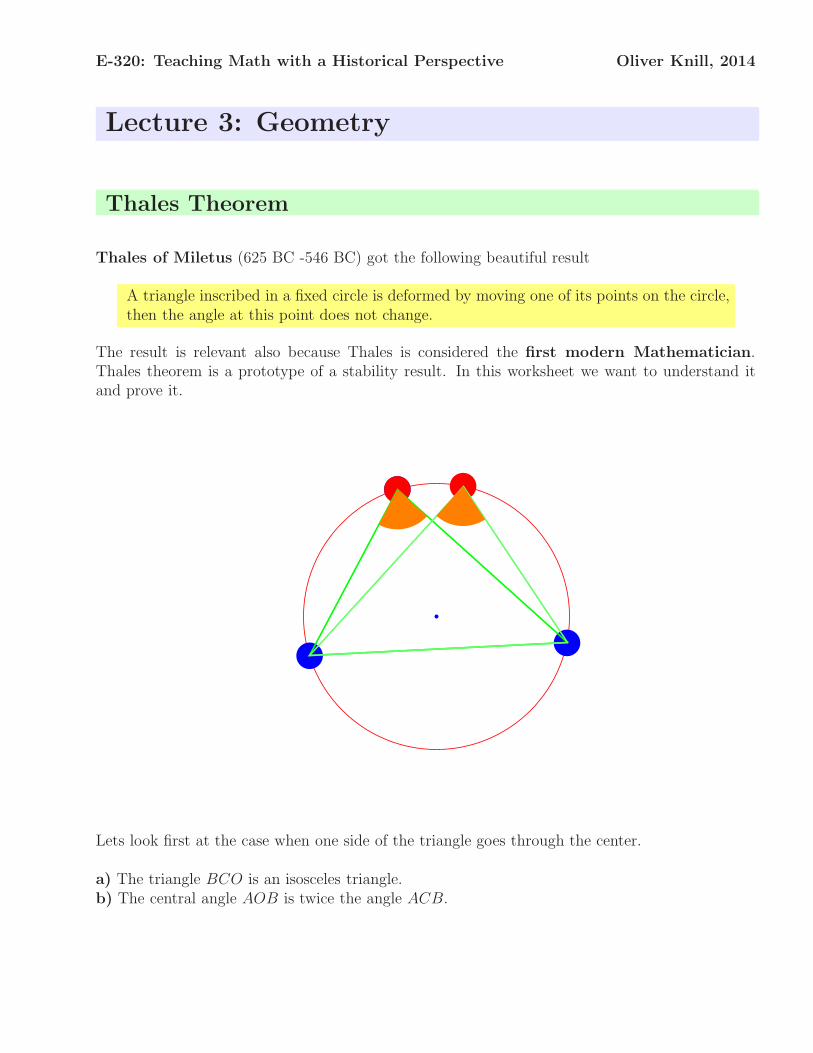
Thales Theorem

Thales of Miletus (625 BC -546 BC) got the following beautiful result

A triangle inscribed in a fixed circle is deformed by moving one of its points on the circle,then the angle at this point does not change.

The result is relevant also because Thales is considered the first modern Mathematician.Thales theorem is a prototype of a stability result. In this worksheet we want to understand itand prove it.

Lets look first at the case when one side of the triangle goes through the center.

a) The triangle BCO is an isosceles triangle.b) The central angle AOB is twice the angle ACB.

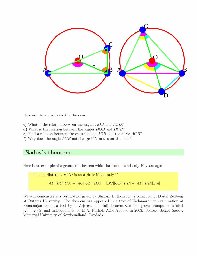
O

C

BA1

1O

D

C

BA

Here are the steps to see the theorem:

c) What is the relation between the angles AOD and ACD?d) What is the relation between the angles DOB and DCB?e) Find a relation between the central angle AOB and the angle ACB?f) Why does the angle ACB not change if C moves on the circle?

Sadov’s theorem

Here is an example of a geometric theorem which has been found only 10 years ago:

The quadrilateral ABCD is on a circle if and only if

|AB||BC||CA|+ |AC||CD||DA| = |BC||CD||DB|+ |AB||BD||DA|

We will demonstrate a verification given by Shalosh B. Ekhadof, a computer of Doron Zeilbergat Rutgers University. The theorem has appeared in a text of Hadamard, an examination ofRamanujan and in a text by J. Vojtech. The full theorem was first proven computer assisted(2003-2005) and independently by M.A. Rashid, A.O. Ajibade in 2003. Source: Sergey Sadov,Memorial University of Newfoundland, Candada.

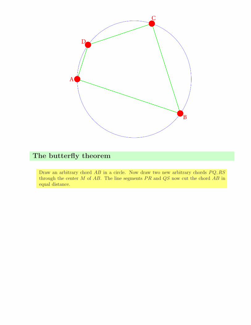
The butterfly theorem

Draw an arbitrary chord AB in a circle. Now draw two new arbitrary chords PQ,RSthrough the center M of AB. The line segments PR and QS now cut the chord AB inequal distance.

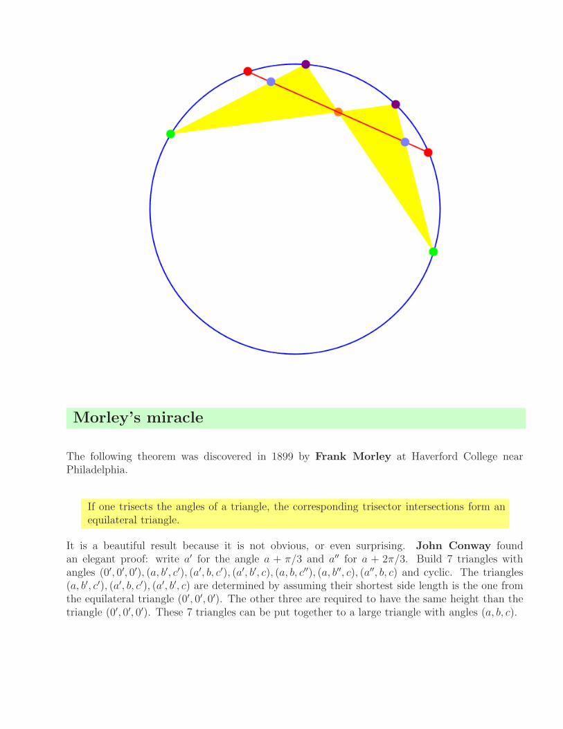
Morley’s miracle

The following theorem was discovered in 1899 by Frank Morley at Haverford College nearPhiladelphia.

If one trisects the angles of a triangle, the corresponding trisector intersections form anequilateral triangle.

It is a beautiful result because it is not obvious, or even surprising. John Conway foundan elegant proof: write a′ for the angle a + π/3 and a′′ for a + 2π/3. Build 7 triangles withangles (0′, 0′, 0′), (a, b′, c′), (a′, b, c′), (a′, b′, c), (a, b, c′′), (a, b′′, c), (a′′, b, c) and cyclic. The triangles(a, b′, c′), (a′, b, c′), (a′, b′, c) are determined by assuming their shortest side length is the one fromthe equilateral triangle (0′, 0′, 0′). The other three are required to have the same height than thetriangle (0′, 0′, 0′). These 7 triangles can be put together to a large triangle with angles (a, b, c).

ΑΑΑ Β

ΒΒ

Γ ΓΓ

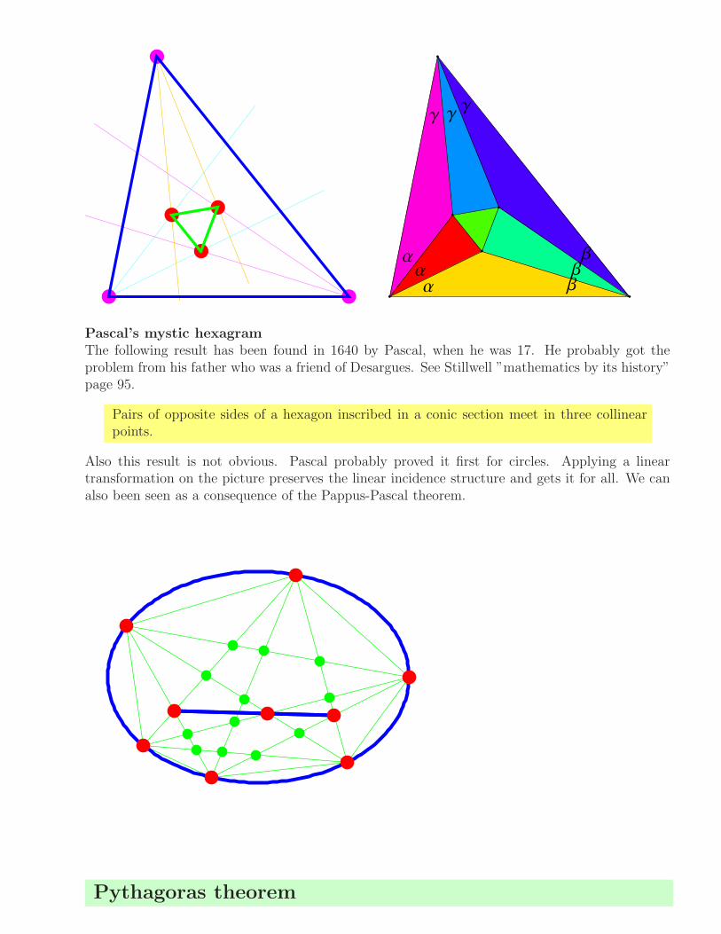
Pascal’s mystic hexagramThe following result has been found in 1640 by Pascal, when he was 17. He probably got theproblem from his father who was a friend of Desargues. See Stillwell ”mathematics by its history”page 95.

Pairs of opposite sides of a hexagon inscribed in a conic section meet in three collinearpoints.

Also this result is not obvious. Pascal probably proved it first for circles. Applying a lineartransformation on the picture preserves the linear incidence structure and gets it for all. We canalso been seen as a consequence of the Pappus-Pascal theorem.

Pythagoras theorem

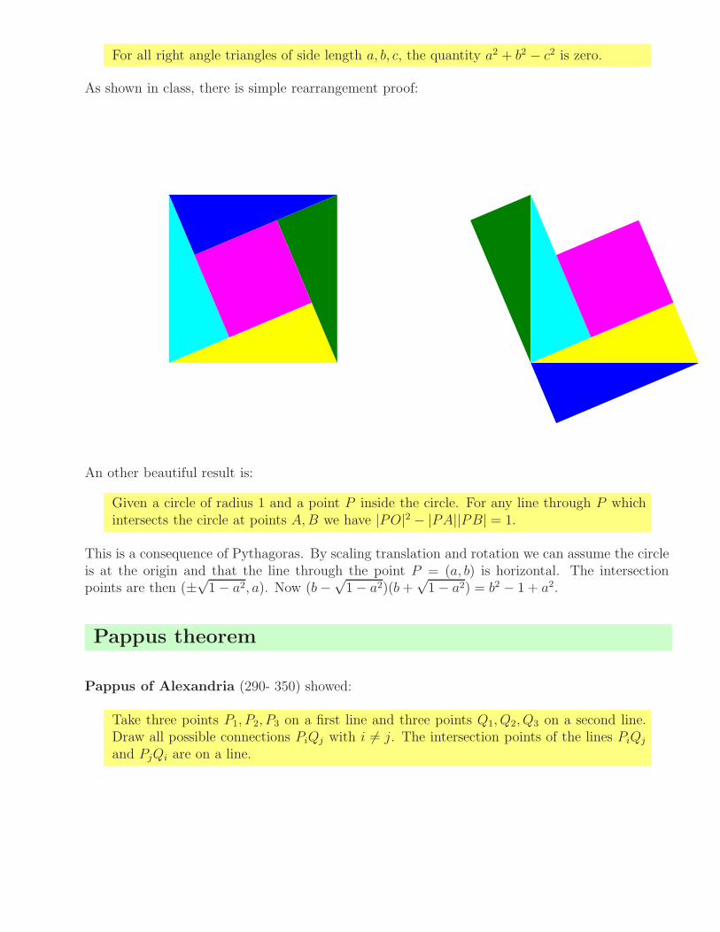
For all right angle triangles of side length a, b, c, the quantity a2 + b2 − c2 is zero.

As shown in class, there is simple rearrangement proof:

An other beautiful result is:

Given a circle of radius 1 and a point P inside the circle. For any line through P whichintersects the circle at points A,B we have |PO|2 − |PA||PB| = 1.

This is a consequence of Pythagoras. By scaling translation and rotation we can assume the circleis at the origin and that the line through the point P = (a, b) is horizontal. The intersectionpoints are then (±

√1− a2, a). Now (b−

√1− a2)(b+

√1− a2) = b2 − 1 + a2.

Pappus theorem

Pappus of Alexandria (290- 350) showed:

Take three points P1, P2, P3 on a first line and three points Q1, Q2, Q3 on a second line.Draw all possible connections PiQj with i 6= j. The intersection points of the lines PiQj

and PjQi are on a line.

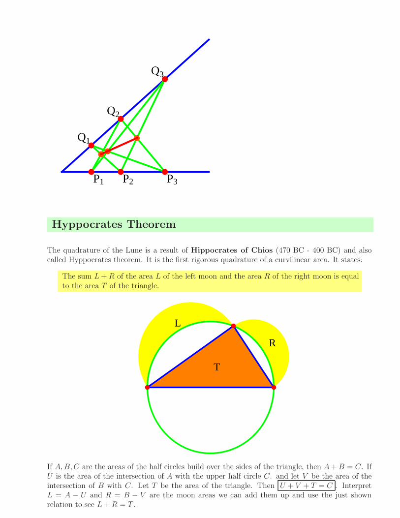
P1 P2 P3

Q1

Q2

Q3

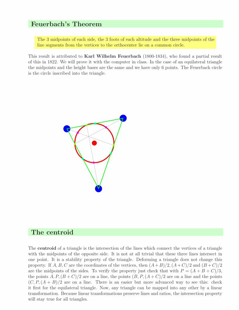
Hyppocrates Theorem

The quadrature of the Lune is a result of Hippocrates of Chios (470 BC - 400 BC) and alsocalled Hyppocrates theorem. It is the first rigorous quadrature of a curvilinear area. It states:

The sum L+R of the area L of the left moon and the area R of the right moon is equalto the area T of the triangle.

R

L

T

If A,B,C are the areas of the half circles build over the sides of the triangle, then A+B = C. IfU is the area of the intersection of A with the upper half circle C. and let V be the area of theintersection of B with C. Let T be the area of the triangle. Then U + V + T = C . InterpretL = A − U and R = B − V are the moon areas we can add them up and use the just shownrelation to see L+R = T .

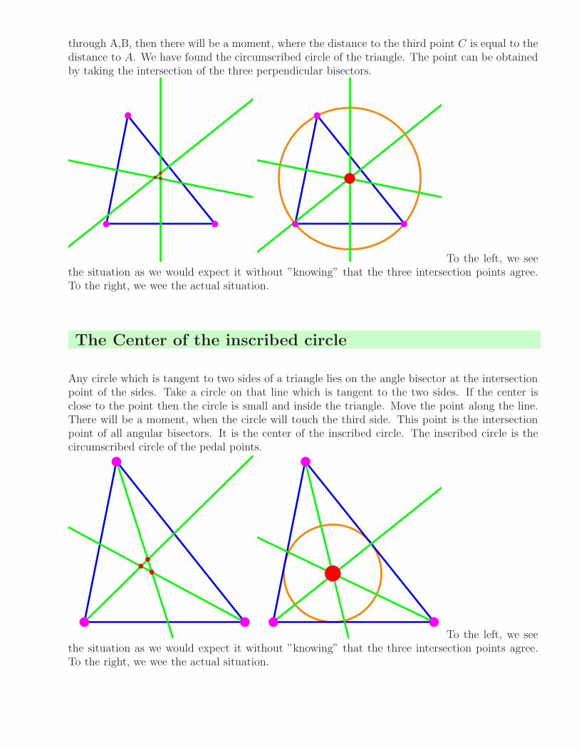
Feuerbach’s Theorem

The 3 midpoints of each side, the 3 foots of each altitude and the three midpoints of theline segments from the vertices to the orthocenter lie on a common circle.

This result is attributed to Karl Wilhelm Feuerbach (1800-1834), who found a partial resultof this in 1822. We will prove it with the computer in class. In the case of an equilateral trianglethe midpoints and the height bases are the same and we have only 6 points. The Feuerbach circleis the circle inscribed into the triangle.

The centroid

The centroid of a triangle is the intersection of the lines which connect the vertices of a trianglewith the midpoints of the opposite side. It is not at all trivial that these three lines intersect inone point. It is a stability property of the triangle. Deforming a triangle does not change thisproperty. If A,B,C are the coordinates of the vertices, then (A+B)/2, (A+C)/2 and (B+C)/2are the midpoints of the sides. To verify the property just check that with P = (A + B + C)/3,the points A, P, (B + C)/2 are on a line, the points (B,P, (A+ C)/2 are on a line and the points(C, P, (A + B)/2 are on a line. There is an easier but more advanced way to see this: checkit first for the equilateral triangle. Now, any triangle can be mapped into any other by a lineartransformation. Because linear transformations preserve lines and ratios, the intersection propertywill stay true for all triangles.

To the left, we seethe situation as we would expect it without ”knowing” that the three intersection points agree.To the right, we wee the actual situation.

The orthocenter

The orthocenter is the intersection of the three altitudes of a triangle. Also here - a priory -we have three different points the intersection, for each pair of altitudes. Why do they meet inone point? It is not obvious and was not proven by the Greeks for example. One can take theintersection of two altitudes, get a point P and form the line from P to the third point in thetriangle. The fact that this line is perpendicular to the third line can be seen by looking at theangles. The angles between to heights is the same than the angle between the two correspondingsides.

To the left, we seethe situation as we would expect it without ”knowing” that the three intersection points agree.To the right, we wee the actual situation.

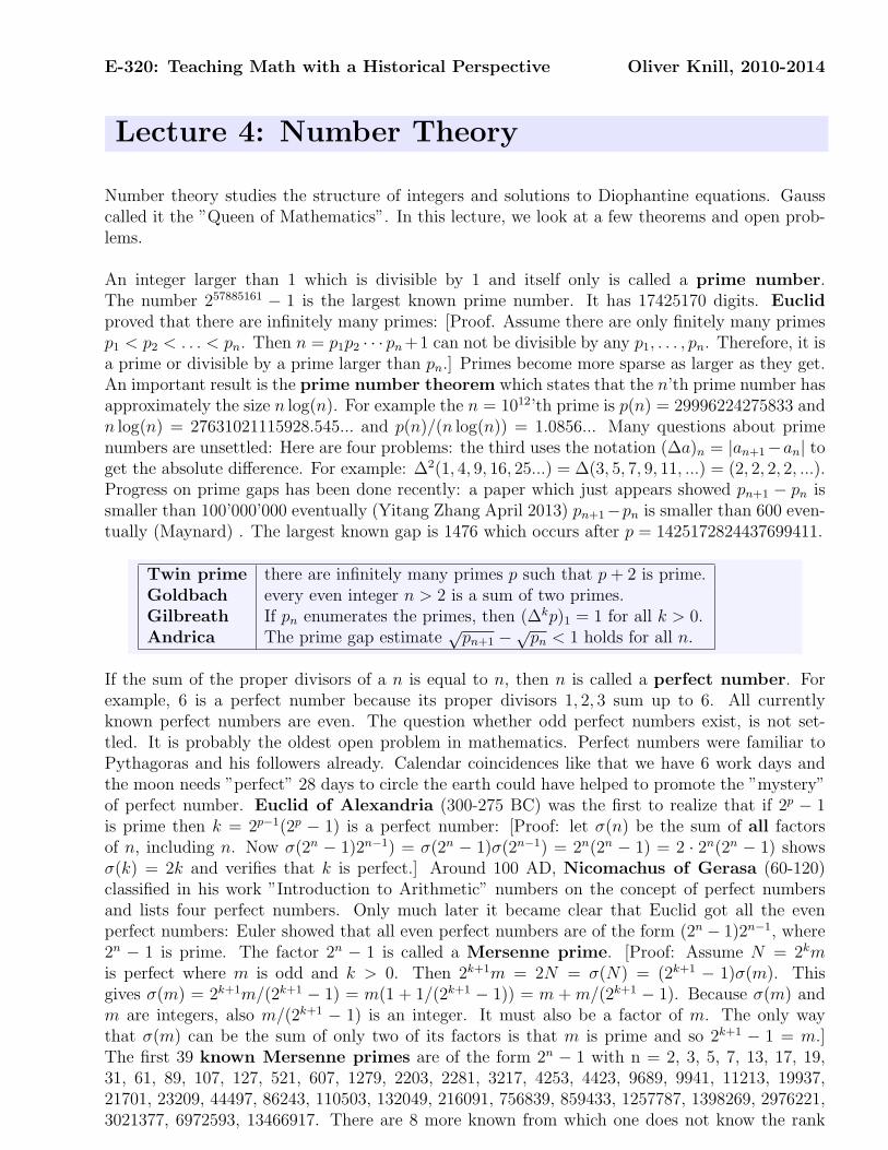
The Center of the Circumscribed circle

Any circle which passes through two points A,B of a triangle lies on the perpendicular bisectorof A and B. When moving a point M on that line and always drawing the circle centered at M

through A,B, then there will be a moment, where the distance to the third point C is equal to thedistance to A. We have found the circumscribed circle of the triangle. The point can be obtainedby taking the intersection of the three perpendicular bisectors.

To the left, we seethe situation as we would expect it without ”knowing” that the three intersection points agree.To the right, we wee the actual situation.

The Center of the inscribed circle

Any circle which is tangent to two sides of a triangle lies on the angle bisector at the intersectionpoint of the sides. Take a circle on that line which is tangent to the two sides. If the center isclose to the point then the circle is small and inside the triangle. Move the point along the line.There will be a moment, when the circle will touch the third side. This point is the intersectionpoint of all angular bisectors. It is the center of the inscribed circle. The inscribed circle is thecircumscribed circle of the pedal points.

To the left, we seethe situation as we would expect it without ”knowing” that the three intersection points agree.To the right, we wee the actual situation.

E-320: Teaching Math with a Historical Perspective Oliver Knill, 2010-2014

Lecture 4: Number Theory

Number theory studies the structure of integers and solutions to Diophantine equations. Gausscalled it the ”Queen of Mathematics”. In this lecture, we look at a few theorems and open prob-lems.

An integer larger than 1 which is divisible by 1 and itself only is called a prime number.The number 257885161 − 1 is the largest known prime number. It has 17425170 digits. Euclid

proved that there are infinitely many primes: [Proof. Assume there are only finitely many primesp1 < p2 < . . . < pn. Then n = p1p2 · · · pn+1 can not be divisible by any p1, . . . , pn. Therefore, it isa prime or divisible by a prime larger than pn.] Primes become more sparse as larger as they get.An important result is the prime number theorem which states that the n’th prime number hasapproximately the size n log(n). For example the n = 1012’th prime is p(n) = 29996224275833 andn log(n) = 27631021115928.545... and p(n)/(n log(n)) = 1.0856... Many questions about primenumbers are unsettled: Here are four problems: the third uses the notation (∆a)n = |an+1−an| toget the absolute difference. For example: ∆2(1, 4, 9, 16, 25...) = ∆(3, 5, 7, 9, 11, ...) = (2, 2, 2, 2, ...).Progress on prime gaps has been done recently: a paper which just appears showed pn+1 − pn issmaller than 100’000’000 eventually (Yitang Zhang April 2013) pn+1−pn is smaller than 600 even-tually (Maynard) . The largest known gap is 1476 which occurs after p = 1425172824437699411.

Twin prime there are infinitely many primes p such that p+ 2 is prime.Goldbach every even integer n > 2 is a sum of two primes.Gilbreath If pn enumerates the primes, then (∆kp)1 = 1 for all k > 0.Andrica The prime gap estimate

√pn+1 −

√pn < 1 holds for all n.

If the sum of the proper divisors of a n is equal to n, then n is called a perfect number. Forexample, 6 is a perfect number because its proper divisors 1, 2, 3 sum up to 6. All currentlyknown perfect numbers are even. The question whether odd perfect numbers exist, is not set-tled. It is probably the oldest open problem in mathematics. Perfect numbers were familiar toPythagoras and his followers already. Calendar coincidences like that we have 6 work days andthe moon needs ”perfect” 28 days to circle the earth could have helped to promote the ”mystery”of perfect number. Euclid of Alexandria (300-275 BC) was the first to realize that if 2p − 1is prime then k = 2p−1(2p − 1) is a perfect number: [Proof: let σ(n) be the sum of all factorsof n, including n. Now σ(2n − 1)2n−1) = σ(2n − 1)σ(2n−1) = 2n(2n − 1) = 2 · 2n(2n − 1) showsσ(k) = 2k and verifies that k is perfect.] Around 100 AD, Nicomachus of Gerasa (60-120)classified in his work ”Introduction to Arithmetic” numbers on the concept of perfect numbersand lists four perfect numbers. Only much later it became clear that Euclid got all the evenperfect numbers: Euler showed that all even perfect numbers are of the form (2n − 1)2n−1, where2n − 1 is prime. The factor 2n − 1 is called a Mersenne prime. [Proof: Assume N = 2kmis perfect where m is odd and k > 0. Then 2k+1m = 2N = σ(N) = (2k+1 − 1)σ(m). Thisgives σ(m) = 2k+1m/(2k+1 − 1) = m(1 + 1/(2k+1 − 1)) = m +m/(2k+1 − 1). Because σ(m) andm are integers, also m/(2k+1 − 1) is an integer. It must also be a factor of m. The only waythat σ(m) can be the sum of only two of its factors is that m is prime and so 2k+1 − 1 = m.]The first 39 known Mersenne primes are of the form 2n − 1 with n = 2, 3, 5, 7, 13, 17, 19,31, 61, 89, 107, 127, 521, 607, 1279, 2203, 2281, 3217, 4253, 4423, 9689, 9941, 11213, 19937,21701, 23209, 44497, 86243, 110503, 132049, 216091, 756839, 859433, 1257787, 1398269, 2976221,3021377, 6972593, 13466917. There are 8 more known from which one does not know the rank

of the corresponding Mersenne prime: n = 20996011, 24036583, 25964951, 30402457, 32582657,37156667, 42643801,43112609,57885161. The last was found in January 2013 only. It is unknownwhether there are infinitely many.

A polynomial equations for which all coefficients and variables are integers is called aDiophantine

equation. The first Diophantine equation studied already by Babilonians is x2 + y2 = z2. Asolution (x, y, z) of this equation in positive integers is called a Pythagorean triple. For example,(3, 4, 5) is a Pythagorean triple. Since 1600 BC, it is known that all solutions to this equationare of the form (x, y, z) = (2st, s2 − t2, s2 + t2) or (x, y, z) = (s2 − t2, 2st, s2 + t2), where s, t aredifferent integers. [Proof. Either x or y has to be even because if both are odd, then the sumx2 + y2 is even but not divisible by 4 but the right hand side is either odd or divisible by 4. Movethe even one, say x2 to the left and write x2 = z2 − y2 = (z − y)(z + y), then the right hand sidecontains a factor 4 and is of the form 4s2t2. Therefore 2s2 = z − y, 2t2 = z + y. Solving for z, ygives z = s2 + t2, y = s2 − t2, x = 2st.]Analyzing Diophantine equations can be difficult. Only 10 years ago, one has established that theFermat equation xn + yn = zn has no solutions with xyz 6= 0 if n > 2. Here are some open

problems for Diophantine equations. Are there nontrivial solutions to the following Diophantineequations?

x6 + y6 + z6 + u6 + v6 = w6 x, y, z, u, v, w > 0x5 + y5 + z5 = w5 x, y, z, w > 0xk + yk = n!zk k ≥ 2, n > 1xa + yb = zc, a, b, c > 2 gcd(a, b, c) = 1

The last equation is called Super Fermat. A Texan banker Andrew Beals once sponsored aprize of 100′000 dollars for a proof or counter example to the statement: ”If xp + yq = zr withp, q, r > 2, then gcd(x, y, z) > 1.”Given a prime like 7 and a number n we can add or subtract multiples of 7 from n to get a numberin 0, 1, 2, 3, 4, 5, 6 . We write for example 19 = 12 mod 7 because 12 and 19 both leave the rest5 when dividing by 7. Or 5 ∗ 6 = 2 mod 7 because 30 leaves the rest 2 when dividing by 7. Themost important theorem in elementary number theory is Fermat’s little theorem which tellsthat if a is an integer and p is prime then ap − a is divisible by p. For example 27 − 2 = 126 isdivisible by 7. [Proof: use induction. For a = 0 it is clear. The binomial expansion shows that(a + 1)p − ap − 1 is divisible by p. This means (a + 1)p − (a + 1) = (ap − a) + mp for some m.By induction, ap − a is divisible by p and so (a + 1)p − (a + 1).] An other beautiful theorem isWilson’s theorem which allows to characterize primes: It tells that (n− 1)!+ 1 is divisible by nif and only if n is a prime number. For example, for n = 5, we verify that 4! + 1 = 25 is divisibleby 5. [Proof: assume n is prime. There are then exactly two numbers 1,−1 for which x2 − 1 isdivisible by n. The other numbers in 1, . . . , n− 1 can be paired as (a, b) with ab = 1. Rearrangingthe product shows (n − 1)! = −1 modulo n. Conversely, if n is not prime, then n = km withk,m < n and (n− 1)! = ...km is divisible by n = km. ]The solution to systems of linear equations like x = 3 (mod 5), x = 2 (mod 7) is given by theChinese remainder theorem. To solve it, continue adding 5 to 3 until we reach a numberwhich leaves rest 2 to 7: on the list 3, 8, 13, 18, 23, 28, 33, 38, the number 23 is the solution. Since5 and 7 have no common divisor, the system of linear equations has a solution.For a given n, how do we solve x2 − yn = 1 for the unknowns y, x? A solution produces a squareroot x of 1 modulo n. For prime n, only x = 1, x = −1 are the solutions. For composite n = pq,more solutions x = r · s where r2 = −1 mod p and s2 = −1 mod q appear. Finding x is equivalentto factor n, because the greatest common divisor of x2 − 1 and n is a factor of n. Factoring

is difficult if the numbers are large. It assures that encryption algorithms work and keepbank accounts and communications safe. Number theory, once the least applied discipline ofmathematics has become one of the most applied one in mathematics.

E-320: Teaching Math with a Historical Perspective Oliver Knill, 2012-2014

Lecture 4: Number Theory

Twin prime conjecture

There are infinitely many prime twins p, p+ 2.

The first twin prime is (3, 5). The largest knownprime twins (p, p + 2) have been found in 2011. It is3756801695685 · 2666669 ± 1. There are analogue prob-lems for cousin primes p, p+4, sexy primes p, p+6 orGermaine primes, where p, 2p+1 are prime. Progress:we know that prime gaps of order 600 or smaller appearinfinitely often. (Work of Zhang,Maynard,Tao)

Goldbach conjecture

Every even integer n > 2 is a sum of two primes.

The Goldbach conjecture has been verified numericallyuntil 4·1018. It is known that every sufficiently large oddnumber is the sum of 3 primes. One believes this ”weakGoldbach conjecture” for 3 primes is true for every oddinteger larger than 7.

Andrica conjecture

The prime gap estimate√pn+1 −

√pn < 1 holds.

For example√p1000−

√p999 =

√7919−

√7907 = 0.067....

An other prime gap estimate conjectures is Polignac’sconjecture claiming that there are infinitely manyprime gaps for every even number n. It is stronger thanthe twin prime conjecture. It includes for example theclaim that there are infinitely many cousin primes orsexy primes. Legendre’s conjecture claims that thereexists a prime between any two perfect squares. Between16 = 42 and 25 = 52, there is the prime 23 for example.

Odd perfect numbers

Probably the oldest open problem in mathematics is thequestion

There is an odd perfect number.

A perfect number is equal to the sum of all its properpositive divisors. Like 6 = 1 + 2 + 3. The search forperfect numbers is related to the search of large primenumbers. The largest prime number known today isp = 243112609 − 1. It is called a Mersenne prime. Everyeven perfect number is of the form 2n−1(2n − 1) where2n − 1 is prime.

Diophantine equations

Many problems about Diophantine equations, equationswith integer solutions are unsettled. Here is an example:

Solve x5 + y5 + z5 = w5 for x, y, z, w ∈ N .

Also x5 + y5 = u5 + v5 has no nontrivial solutions yet.Probabilistic considerations suggest that there are nosolutions. The analogue equation x4 + y4 + z4 = w4

had been settled by Noam Elkies in 1988 who found theidentity 26824404+153656394+187967604 = 206156734.

ABC Conjecture

The abc conjecture is:

If a+ b = c, then c ≤ (∏

p|abc p)2.

For example, for 10+22 = 32, the prime factors of abc =7040 are 2, 5, 11 and indeed 32 ≤ (2 ∗ 5 ∗ 11)2 = 12100.The abc-conjecture is open but implies Fermat’s theo-rem for n ≥ 6: assume xn+yn = zn with coprime x, y, z.Take a = xn, b = yn, c = zn. The abc-conjecture giveszn ≤ (

∏p|abc p) ≤ (abc)2 < z6 establishing Fermat for

n ≥ 6. The cases n = 3, 4, 5 to Fermat have been knownfor a long time. In August 2012, there were rumors ofan attack by Shinichi Mochizuki. During 2013 variousmathematicians have tried to understand and verify thetheory.

E-320: Teaching Math with a Historical Perspective Oliver Knill, 2010-2014

Lecture 5: Algebra

Algebra is the theory of algebraic structures like ”groups” and ”rings”. The theory allows tosolve polynomial equations, characterize objects by its symmetries and is the heart and soul ofmany puzzles.Lagrange claims Diophantus to be the inventor of Algebra, others argue that the subject startedwith solutions of quadratic equation by Mohammed ben Musa Al-Khwarizmi in the bookAl-jabr w’al muqabala of 830 AD. Solutions to equation like x2 + 10x = 39 are solved there bycompleting the squares: add 25 on both sides go get x2 + 10x+ 25 = 64 and so (x+ 5) = 8 sothat x = 3.The use of variables introduced in school in elementary algebra were introduced later. Ancienttexts dealt with particular examples. Calculations were done with concrete numbers in the realmof arithmetic. Francois Viete (1540-1603) used first letters like A,B,C,X for variables.

The search for formulas for polynomial equations of degree 3 and 4 lasted 700 years. In the16’th century only the cubic equation and quartic equations were solved. Niccolo Tartaglia andGerolamo Cardano reduced the cubic to the quadratic: [first remove the quadratic part withX = x−a/3 so that X3+aX2+bX+c becomes the depressed cubic x3+px+q. Now substitutex = u− p/(3u) to get a quadratic equation (u6 + qu3

− p3/27)/u3 = 0 for u3.] Lodovico Ferrari

shows that the quartic equation can be reduced to the cubic. For the quintic however no formulascould be found. It was Paolo Ruffini, Niels Abel and Evariste Galois who independentlyrealized that there are no formulas in terms of roots which allow to ”solve” equations p(x) = 0 forpolynomials p of degree larger than 4. This was an amazing achievement and the birth of ”grouptheory”.

Two important algebraic structures are groups and rings.

In a group G one has an operation ∗, an inverse a−1 and a one-element 1 such that a ∗ (b ∗ c) =(a ∗ b) ∗ c, a ∗ 1 = 1 ∗ a = a, a ∗ a−1 = a−1

∗ a = 1. For example, the set Q∗ of nonzero fractionsp/q with multiplication operation ∗ and inverse 1/a form a group. The integers with addition andinverse a−1 = −a and ”1”-element 0 form a group too. A ring R has two compositions + and ∗,where the plus operation is a group satisfying a + b = b+ a in which the one element is called 0.The multiplication operation ∗ has all group properties on R∗ except the existence of an inverse.The two operations + and ∗ are glued together by the distributive law a ∗ (b+ c) = a ∗ b+ a ∗ c.An example of a ring are the integers or the rational numbers or the real numbers. Thelater two are actually fields, rings for which the multiplication on nonzero elements is a grouptoo. The ring of integers are no field because an integer like 5 has no multiplicative inverse. Thering of rational numbers however form a field.

Why is the theory of groups and rings not part of arithmetic? First of all, a crucial ingredientof algebra is the appearance of variables and computations with these algebras without usingconcrete numbers. Second, the algebraic structures are not restricted to ”numbers”. Groups andrings are general structures and extend for example to objects like the set of all possible sym-metries of a geometric object. The set of all similarity operations on the plane for exampleform a group. An important example of a ring is the polynomial ring of all polynomials. Givenany ring R and a variable x, the set R[x] consists of all polynomials with coefficients in R. The

factor a given polynomial with integer coefficients into polynomials of smaller degree: x2− x+ 2

for example can be written as (x+1)(x−2) have a number theoretical flavor. Because symmetriesof some structure form a group, we also have intimate connections with geometry. But this isnot the only connection with geometry. Geometry also enters through the polynomial rings withseveral variables. Solutions to f(x, y) = 0 leads to geometric objects with shape and symmetrywhich sometimes even have their own algebraic structure. They are called varieties, a centralobject in algebraic geometry.

Arithmetic introduces addition and multiplication of numbers. Both form a group. The operationscan be written additively or multiplicatively. Lets look at this a bit closer:For integers, fractions and reals and the addition +, the 1 element 0 and inverse −g, we have agroup. Many groups are written multiplicatively where the 1 element is 1. In the case of fractionsor reals, 0 is not part of the multiplicative group because it is not possible to divide by 0. Thenonzero fractions or the nonzero reals form a group. In all these examples the groups satisfy thecommutative law g ∗ h = h ∗ g.Here is a group which is not commutative: let G be the set of all rotations in space, whichleave the unit cube invariant. There are 3*3=9 rotations around each major coordinate axes,then 6 rotations around axes connecting midpoints of opposite edges, then 2*4 rotations arounddiagonals. Together with the identity rotation e, these are 24 rotations. The group operation isthe composition of these transformations.An other example of a group is S4, the set of all permutations of four numbers (1, 2, 3, 4). Ifg : (1, 2, 3, 4) → (2, 3, 4, 1) is a permutation and h : (1, 2, 3, 4) → (3, 1, 2, 4) is an other permutation,then we can combine the two and define h ∗ g as the permutation which does first g and then h.We end up with the permutation (1, 2, 3, 4) → (1, 2, 4, 3). The rotational symmetry group of thecube happens to be the same than the group S4. To see this ”isomorphism”, label the 4 spacediagonals in the cube by 1, 2, 3, 4. Given a rotation, we can look at the induced permutation ofthe diagonals and every rotation corresponds to exactly one permutation. The symmetry groupcan be introduced for any geometric object. For shapes like the triangle, the cube, the octahedronor tilings in the plane.

Symmetry groups describe geometric shapes by algebra.

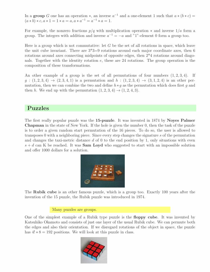
Many puzzles are groups. For a long time, a popular puzzle was the 15-puzzle. It was inventedin 1874 by Noyes Palmer Chapman in the state of New York. If the hole is given the number0, then the task of the puzzle is to order a given random start permutation of the 16 pieces. Todo so, the user is allowed to transposes 0 with a neighboring piece. Since every step changes thesignature s of the permutation and changes the taxi-metric distance d of 0 to the end position by1, only situations with even s+ d can be reached. It was Sam Loyd who suggested to start withan impossible solution and as an evil plot to offer 1000 dollars for a solution. The Rubik cube

is an other famous puzzle, which is a group too. Exactly 100 years after the invention of the 15puzzle, the Rubik puzzle was introduced in 1974. Its still popular and the world record is to haveit solved in 5.55 seconds. Cubes 2x2x2 to 7x7x7 have been solved in a total time of 6 minutes.

Many puzzles are groups.

A small version is the ”floppy”, which is a third of the rubik and which has only 192 elements. Wewill look in class also at Meffert’s great challenge. Probably the simplest example of a Rubiktype puzzle is the pyramorphix. It is a puzzle based on the tetrahedron. Its group has only24 elements. It is the group of all possible permutations of the 4 elements. It is the same groupas the group of all reflection and rotation symmetries of the cube in three dimensions and alsois relevant when understanding the solutions to the quartic equation discussed at the beginning.

E-320: Teaching Math with a Historical Perspective Oliver Knill, 2014

Lecture 5: Algebra

Quadratic equation

The quadratic equation x2 + bx+ c = 0 can be solved by completing the square. This idea is dueto Mohammed ben Musa Al-Khwarizmi:

x =−b+

√b2 − 4c

2

Example: : x2 − 4x− 5 has the root (4 +√16 + 20)/2 = 5 or (4−

√16 + 20)/2 = −1.

The use of variables and so elementary algebra was introduced only in the 16’th century.

1 The cubic equation

Niccolo Tartaglia and Gerolamo Cardano have shown how to solve the cubic equation X3 +aX2 + bX + c = 0.

Write X = x− a/3 to get the depressed cubic x3 + px+ q. Withx = u−p/(3u), we get the quadratic equation (u6+qu3−p3/27) = 0.

Example: : Start with X3+2X2−13X+10 = 0. With X = x−2/3 we get x3−43x/3+520/27.

With x = u+43/(9u) we end up with u6+520u3/27+79507/729 = 0 which is a quadratic equationfor u3.

2 The quartic

Lodovico Ferrari shows that the quartic equation can be reduced to the cubic. For quintic

equations, no formulas could be found.

3 The cubic

It was Paolo Ruffini, Niels Abel and Evariste Galois who realized that there are no formulasin general in terms of roots if the degree of the polynomial is 5 or higher. This was a triumph ofgroup theory.

There are no formulas in general for the solution of polynomialequations of degree 5 or higher.

Symmetry groups

In a group G one has an operation ∗, an inverse a−1 and a one-element 1 such that a ∗ (b ∗ c) =(a ∗ b) ∗ c, a ∗ 1 = 1 ∗ a = a, a ∗ a−1 = a−1 ∗ a = 1.

For example, the nonzero fractions p/q with multiplication operation ∗ and inverse 1/a form agroup. The integers with addition and inverse a−1 = −a and ”1”-element 0 form a group too.

Here is a group which is not commutative: let G be the set of all rotations in space, which leavethe unit cube invariant. There are 3*3=9 rotations around each major coordinate axes, then 6rotations around axes connecting midpoints of opposite edges, then 2*4 rotations around diago-nals. Together with the identity rotation e, these are 24 rotations. The group operation is thecomposition of these transformations.

An other example of a group is the set of all permutations of four numbers (1, 2, 3, 4). Ifg : (1, 2, 3, 4) → (2, 3, 4, 1) is a permutation and h : (1, 2, 3, 4) → (3, 1, 2, 4) is an other per-mutation, then we can combine the two and define h∗ g as the permutation which does first g andthen h. We end up with the permutation (1, 2, 3, 4) → (1, 2, 4, 3).

Puzzles

The first really popular puzzle was the 15-puzzle. It was invented in 1874 by Noyes Palmer

Chapman in the state of New York. If the hole is given the number 0, then the task of the puzzleis to order a given random start permutation of the 16 pieces. To do so, the user is allowed totransposes 0 with a neighboring piece. Since every step changes the signature s of the permutationand changes the taxi-metric distance d of 0 to the end position by 1, only situations with evens + d can K be reached. It was Sam Loyd who suggested to start with an impossible solutionand offer 1000 dollars for a solution.

The Rubik cube is an other famous puzzle, which is a group too. Exactly 100 years after theinvention of the 15 puzzle, the Rubik puzzle was introduced in 1974.

Many puzzles are groups.

One of the simplest example of a Rubik type puzzle is the floppy cube. It was invented byKatsuhiko Okamoto and consists of just one layer of the usual Rubik cube. We can permute boththe edges and also their orientation. If we disregard rotations of the object in space, the puzzlehas 4! ∗ 8 = 192 positions. We will look at this puzzle in class.

E-320: Teaching Math with a Historical Perspective Oliver Knill, 2010-2014

Lecture 6: Calculus

Calculus formalizes the process of taking differences and taking sums. Differences measurechange, sums explore how things accumulate. The process of taking differences has a limitcalled derivative. The process of taking sums will lead to the integral. These two processes arerelated in an intimate way. In this lecture, we look at these two processes in the simplest possiblesetup, where functions are evaluated on integers and where we do not take any limits.Several dozen thousand years ago, numbers were represented by units like

1, 1, 1, 1, 1, 1, . . .

for example carved in the Ishango bone. It took thousands of years until numbers were representedwith symbols like

0, 1, 2, 3, 4, . . . .

Using the modern concept of function, we can say f(0) = 0, f(1) = 1, f(2) = 2, f(3) = 3 andmean that the function f assigns to an input like 1001 an output like f(1001) = 1001. Lets callDf(n) = f(n + 1)− f(n) the difference between two function values. We see that the functionf satisfies Df(n) = 1 for all n. We can also formalize the summation process. If g(n) = 1 is thefunction which is constant 1, then Sg(n) = g(0)+ g(1)+ . . .+ g(n− 1) = 1+ 1+ · · ·+1 = n. Wesee that Df = g and Sg = f . Lets start with f(n) = n and apply summation on that function:

Sf(n) = f(0) + f(1) + f(2) + · · ·+ f(n− 1) .

In our example, we get the values:

0, 1, 3, 6, 10, 15, 21, . . . .

The new function g = Sf satisfies g(1) = 1, g(2) = 3, g(2) = 6, etc. These numbers are calledtriangular numbers. From g we can get back f by taking difference:

Dg(n) = g(n+ 1)− g(n) = f(n) .

For example Dg(5) = g(6)− g(5) = 15 − 10 = 5 which indeed is f(5). Finding a formula for thesum Sf(n) is not so easy. Can you do it? When Karl-Friedrich Gauss was a 9 year old schoolkid, his teacher, a Mr. Buttner gave him the task to sum up the first 100 numbers 1+2+ · · ·+100.Gauss found the answer immediately by pairing things up: to add up 1 + 2 + 3 + . . . + 100 hewould write this as (1 + 100) + (2 + 99) + · · · + (50 + 51) leading to 50 terms of 101 to getfor n = 101 the value g(n) = n(n − 1)/2 = 5050. Taking differences again is easier Dg(n) =n(n + 1)/2− n(n− 1)/2 = n = f(n).Lets add now the triangular numbers up compute h = Sg. We get the sequence

0, 1, 4, 10, 20, 35, ...

called the tetrahedral numbers. One can h(n) balls to build a tetrahedron of side length n.For example, h(4) = 20 golf balls are needed to build a tetrahedron of side length 4. The formula

which holds for h is h(n) = n(n− 1)(n− 2)/6 . Here is the fundamental theorem of calculus,

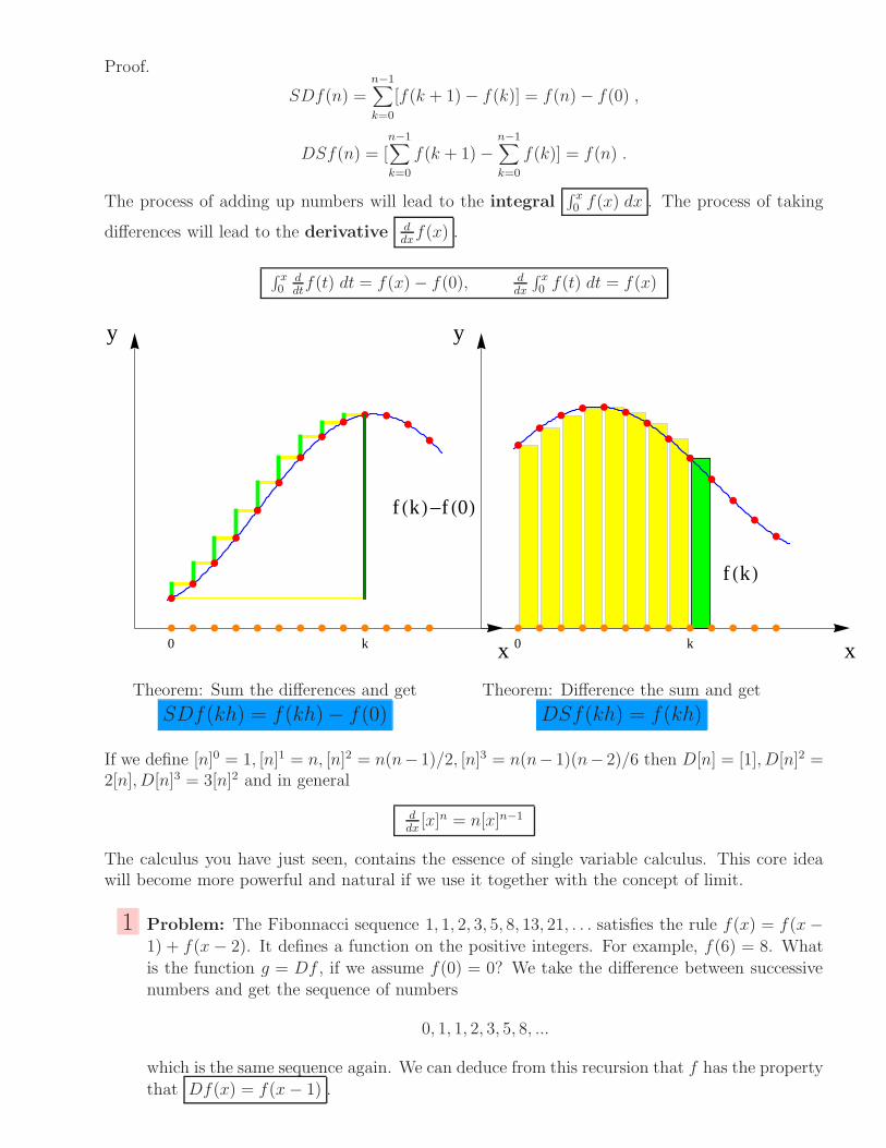
which is the core of calculus:SDf(n) = f(n)− f(0), DSf(n) = f(n) .

Proof.

SDf(n) =n−1∑

k=0

[f(k + 1)− f(k)] = f(n)− f(0) ,

DSf(n) = [n−1∑

k=0

f(k + 1)−n−1∑

k=0

f(k)] = f(n) .

The process of adding up numbers will lead to the integral∫x

0 f(x) dx . The process of taking

differences will lead to the derivative d

dxf(x) .

∫x

0d

dtf(t) dt = f(x)− f(0), d

dx

∫x

0 f(t) dt = f(x)

k x

y

0

f HkL-f H0L

k x

y

0

f HkL

Theorem: Sum the differences and get

SDf(kh) = f(kh)− f(0)Theorem: Difference the sum and get

DSf(kh) = f(kh)

If we define [n]0 = 1, [n]1 = n, [n]2 = n(n− 1)/2, [n]3 = n(n− 1)(n− 2)/6 then D[n] = [1], D[n]2 =2[n], D[n]3 = 3[n]2 and in general

d

dx[x]n = n[x]n−1

The calculus you have just seen, contains the essence of single variable calculus. This core ideawill become more powerful and natural if we use it together with the concept of limit.

1 Problem: The Fibonnacci sequence 1, 1, 2, 3, 5, 8, 13, 21, . . . satisfies the rule f(x) = f(x−

1) + f(x− 2). It defines a function on the positive integers. For example, f(6) = 8. What

is the function g = Df , if we assume f(0) = 0? We take the difference between successivenumbers and get the sequence of numbers

0, 1, 1, 2, 3, 5, 8, ...

which is the same sequence again. We can deduce from this recursion that f has the property

that Df(x) = f(x− 1) .

2 Problem: Take the same function f given by the sequence 1, 1, 2, 3, 5, 8, 13, 21, ... but now

compute the function h(n) = Sf(n) obtained by summing the first n numbers up. It givesthe sequence 1, 2, 4, 7, 12, 20, 33, .... What sequence is that?

Solution: Because Df(x) = f(x − 1) we have f(x) − f(0) = SDf(x) = Sf(x − 1) sothat Sf(x) = f(x+ 1)− f(1). Summing the Fibonnacci sequence produces the Fibonnacci

sequence shifted to the left with f(2) = 1 is subtracted. It has been relatively easy to findthe sum, because we knew what the difference operation did. This example shows:

We can study differences to understand sums.

The next problem illustrates this too:

3 Problem: Find the next term in the sequence2 6 12 20 30 42 56 72 90 110 132 . Solution: Take differences

2 6 12 20 30 42 56 72 90 110 132

2 4 6 8 10 12 14 16 18 20 222 2 2 2 2 2 2 2 2 2 2

0 0 0 0 0 0 0 0 0 0 0

.

Now we can add an additional number, starting from the bottom and working us up.

2 6 12 20 30 42 56 72 90 110 132 156

2 4 6 8 10 12 14 16 18 20 22 24

2 2 2 2 2 2 2 2 2 2 2 2

0 0 0 0 0 0 0 0 0 0 0 0

4 Problem: The function f(n) = 2n is called the exponential function. We have forexample f(0) = 1, f(1) = 2, f(2) = 4, . . .. It leads to the sequence of numbers

n= 0 1 2 3 4 5 6 7 8 . . .

f(n)= 1 2 4 8 16 32 64 128 256 . . .

We can verify that f satisfies the equation Df(x) = f(x) . because Df(x) = 2x+1 − 2x =

(2− 1)2x = 2x.

This is an important special case of the fact that

The derivative of the exponential function is the exponential function itself.

The function 2x is a special case of the exponential function when the Planck constant is

equal to 1. We will see that the relation will hold for any h > 0 and also in the limith → 0, where it becomes the classical exponential function ex which plays an important role

in science.

Calculus has many applications: computing areas, volumes, solving differential equations. It evenhas applications in arithmetic. Here is an example for illustration. It is a proof that π is irrational.This is especially appropriete since next Friday is π day!

We show here the proof by Ivan Niven is given in a book of Niven-Zuckerman-Montgomery.It originally appeared in 1947 (Ivan Niven, Bull.Amer.Math.Soc. 53 (1947),509). The proofillustrates how calculus can help to get results in arithmetic.Proof. Assume π = a/b with positive integers a and b. For any positive integer n define

f(x) = xn(a− bx)n/n! .

We have f(x) = f(π − x) and0 ≤ f(x) ≤ πnan/n!(∗)

for 0 ≤ x ≤ π. For all 0 ≤ j ≤ n, the j-th derivative of f is zero at 0 and π and for n <= j, thej-th derivative of f is an integer at 0 and π.

The functionF (x) = f(x)− f (2)(x) + f (4)(x)− ...+ (−1)nf (2n)(x)

has the property that F (0) and F (π) are integers and F + F ′′ = f . Therefore, (F ′(x) sin(x) −F (x) cos(x))′ = f sin(x). By the fundamental theorem of calculus,

∫π

0 f(x) sin(x) dx is an integer.Inequality (*) implies however that this integral is between 0 and 1 for large enough n. For suchan n we get a contradiction.

E-320: Teaching Math with a Historical Perspective Oliver Knill, 2010-2014

Lecture 7: Set Theory and Logic

Set theory studies sets, the fundamental building blocks of mathematics. While logic describesthe language of all mathematics, set theory provides the framework for additional structures.

In Cantorian set theory, one can compute with subsets of a given set X like with numbers.There are two basic operations: the addition A+B of two sets is defined as the set of all pointswhich are in exactly one of the sets. The multiplication A · B of two sets contains all thepoints which are in both sets. With the symmetric difference as addition and the intersectionas multiplication, the subsets of a given set X become a ring. One calls it a Boolean ring.It has the property A + A = 0 and A · A = A for all sets. The zero element is the empty set∅ = . The additive inverse of A is the complement −A of A in X . The multiplicative 1-elementis the set X because X ·A = A. As in the ring of integers, the addition and multiplication on setsis commutative and multiplication does not have an inverse in general. We will play with this ring.

Two sets A,B have the same cardinality, if there exists a one-to-one map from A to B. Forfinite sets, this means that they have the same number of elements. Sets which do not have finitelymany elements are called infinite. Do all sets with infinitely many elements have the same car-dinality? The integers Z and the natural numbers N for example are infinite sets which havethe same cardinality: f(2n) = n, f(2n + 1) = −n establishes a bijection between N and Z. Alsothe rational numbers Q have the same cardinality than N . Associate a fraction p/q with a point(p, q) in the plane. Now cut out the column q = 0 and run the Ulam spiral on the modified plane.This provides a numbering of the rationals. Sets which can be counted are called of cardinality ℵ0.

Does an interval have the same cardinality than the reals? Even so an interval like (−π/2, π/2)has finite length, one can bijectively map it to the real lines with the tan map. Similarly onecan see that any two intervals of positive length have the same cardinality. It was a great mo-ment of mathematics, when Georg Cantor realized in 1874 that the interval (0, 1) does not havethe same cardinality than the natural numbers. His argument is ingenious: assume, we couldcount the points a1, a2, . . .. If 0.ai1ai2ai3... is the decimal expansion of ai, define the real numberb = 0.b1b2b3..., where bi = aii + 1 mod 10. Because this number b does not agree at the firstdecimal place with a1, at the second place with a2 and so on, the number b does not appear inthat enumeration of all reals. It has positive distance at least 10−i from the i’th number (and anyrepresentation of the number by a decimal expansion which is equivalent). This is a contradiction.The new cardinality, the continuum is also denoted ℵ1. The reals are uncountable. This giveselegant proofs like the existence of transcendental number, numbers which are not algebraic,the root of any polynomial with integer coefficients: algebraic numbers can be counted.

Similarly as one could establish a bijection between the natural numbers N and the integers Z,there is a bijection f between the interval I and the unit square: if x = 0.x1x2x3... is the decimalexpansion of x then f(x) = (0.x1x3x5 . . . , 0.x2x4x6 . . .) is the bijection. Are there cardinalitiesabove ℵ0 and ℵ1? Cantor answered also this question. He showed that for an infinite set, the setof all subsets has a larger cardinality than the set itself. How does one see this? Assume there is abijection x → A(x) which maps each point to a set A(x). Now look at the set B = x | x /∈ A(x) and let b be the point in X which corresponds to B. If y ∈ B, then y /∈ B(x). On the other hand,if y /∈ B, then y ∈ B. The set B does appear in the ”enumeration” x → A(x) of all sets. The set

from P (N) to [0, 1]. The set of all finite subsets of N however can be counted. The set of allsubsets of the real numbers has cardinality ℵ2, etc.

Is there a cardinality between ℵ0 and ℵ1? In other words, is there a set which can not be countedand which is strictly smaller than the continuum in the sense that one can not find a bijectionbetween it and R? This was the first of the 23 problems posed by Hilbert in 1900. The answeris surprising: one has a choice. One can accept either the ”yes” or the ”no” as a new axiom.In both cases, Mathematics is still fine. The nonexistence of a cardinality between ℵ0 and ℵ1 iscalled the continuum hypothesis and is usually abbreviated CH. It is independent of the otheraxioms making up mathematics. This was the work of Kurt Godel in 1940 and Paul Cohenin 1963. For most mathematical questions, it does not matter whether one accepts CH or not.The story of exploring the consistency and completeness of axiom systems of all of mathematicsis exciting. Euclid axiomatized all of Euclidean geometry, Hilbert’s goal was much more ambi-tious, to find a set of axiom systems for all of mathematics. The challenge to prove Euclid’s5’th postulate is paralleled by the quest to prove the CH. But the later is much more funda-mental and striking because it deals with all of mathematics and not only with a particularfield of geometry. Here are the Zermelo-Frenkel Axioms (ZFC) including the Axiom of choice(C) as established by Ernst Zermelo in 1908 and Adolf Fraenkel and Thoral Skolem in 1922.

Extension If two sets have the same elements, they are the same.Image Given a function and a set, then the image of the function is a set too.Pairing For any two sets, there exists a set which contains both sets.Property For any property, there exists a set for which each element has the property.Union Given a set of sets, there exists a set which is the union of these sets.Power Given a set, there exists the set of all subsets of this set.Infinity There exists an infinite set.Regularity Every nonempty set has an element which has no intersection with the set.Choice Any set of nonempty sets leads to a set which contains an element from each.

The axiom of choice (C) has a nonconstructive nature which can lead to seemingly paradoxicalresults like the Banach Tarski paradox: one can cut the unit ball into 5 pieces, rotate andtranslate the pieces to assemble two identical balls of the same size than the original ball. Godeland Cohen showed that the axiom of choice is logically independent of the other axioms ZF. Otheraxioms in ZF have been shown to be independent, like the axiom of infinity. A finitist wouldrefute this axiom and work without it. It is surprising what one can do with finite sets. The axiomof regularity excludes Russellian sets like the set X of all sets which do not contain themselves.The Russell paradox is: Does X contain X? It is popularized as the Barber riddle: a bar-ber in a town only shaves the people who do not shave themselves. Does the barber shave himself?

A complete axiomatization of mathematics is never complete because of Godels theorems of1931. They deal with mathematical theories. They are assumed to be sufficiently strongmeaning that one can do at least basic arithmetic in them and call it simply a theory:

First incompleteness theorem:In any theory there are true statementswhich can not be proved within the theory.

Second incompleteness theorem:In any theory, the consistency of the theorycan not be proven within the theory.

The proof uses an encoding of mathematical sentences which allows to state liar paradoxicalstatement ”this sentence can not be proved”. While the later is an odd recreational entertainmentgag, it is the core for a theorem which makes striking statements about mathematics. Thesetheorems are not limitations of mathematics; they illustrate its infiniteness. How awful if onecould build axiom system and enumerate mechanically all possible truths from it.

E-320: Teaching Math with a Historical Perspective Oliver Knill, 2014

Lecture 7: Set Theory and Logic

We will mostly focus on the work of two mathematicians: Georg Cantor and Kurt Godel.Their mathematics changed our way we think about mathematics. In both cases, the mathematicscommunity needed time to absorb the implications of the revolutions.Hilbert said about Cantor ”Nobody will drive us from the paradise that Cantor has created for us”.Cantor clarified the term ”cardinality” is, showed that certain infinities like that the cardinalityof points in the plane or points in space are the same and most importantly showed that differentinfinities exist. Godels theorems show that mathematics and knowledge in general can not beexhausted by listing a sequence of basic truths from which everything follows. Whenever we makesuch a list, there are statements which are independent of the system. It would be a mistake totake this as a limitation of mathematics, in contrary it shows that mathematics is inexhaustible:there is always something more to explore.

Counting: Set theory

We first demonstrate that one can compute with sets like with numbers. There is an addition, thesymmetric difference and a multiplication, the intersection. With these two operations, we provethe familiar rules of arithmetic

A+B = B + A,A · B = B · A,A · (B + C) = A · B + A · C

hold. This is a Boolean algebra. There is a set which plays the role of 0. Which one is it? Thereis also a set which plays the role of 1. Which one is it?

Counting: Hilbert’s Hotel

Hilbert’s hotel is located on route 8. It has countably many rooms numbered 1, 2, 3, . . .. Thehotel is fully booked. As a newcomer arrives. David, the hotel manager is mortified. David hasan idea and moves guest in room i to room i+ 1 and gives the newcomer the first room 1.

An other day, the hotel is empty but a large group arrives. They are the ”fractions” on their wayto a cardinal match with the ”squares”. Can David accommodate them? He thinks hard andfinally manages.

In the summer, the ”reals” appear. David is not there but has George, the apprentice is in theoffice. The group consists of all real numbers between 0 and 1. Can George accomodate them?As much as he tries to shift and renumber, he can not do it.

Counting: the interval

The interval (−1, 1) has the same cardinality than the real line. The function f(x) = tan(πx/2)maps the interval (−1, 1) onto the real line, one to one.

The square (0, 1)×(0, 1) has the same cardinality than the real line. A bijection can be constructedby f(0.a1a2a3a4...) = (0.a1a3a5, 0.a2a4a6...).

Arithmetic with sets

One can calculate with sets as with numbers. They form a ”Boolean ring”.

Addition: A+B = A∆B with the zero element ∅Multiplication: A · B = A ∩ B with the one element Ω.

All the rules of the real numbers apply but there are additional consequences which appear a bitstrange A+ A = 0 and A2 = A · A = A. This means that A is its own additive inverse.

Paradoxa

We have seen a few paradoxa like the Liars paradox ”I lie”, the barbers paradox ”the barberis the person who shaves everybody who does not shave him or herself”, the surprise examproblem ”it is impossible to make a surprise exam problem”, the heap problem ”take a grainaway from a heap keeps it a heap”, the biographer’s problem ”who needs one year to write oneday of his biography”, Here is an other, the Berry paradox which comes somehow close to theGoedel numbering:

The smallest integer not definable in less than 11 words.

The problem is that this number is defined with 10 words. This looks like a stupid example butit illustrates that there are properties of numbers like ”the shortest way to describe the number”which is not computable.

Axiom of choice

The axiom of choice (C) has a nonconstructive nature which can lead to seemingly paradoxicalresults like the Banach Tarski paradox: one can cut the unit ball into 5 pieces, rotate andtranslate the pieces to assemble two identical balls of the same size than the original ball. Godeland Cohen showed that the axiom of choice is logically independent of the other axioms ZF.

E-320: Teaching Math with a Historical Perspective Oliver Knill, 2010-2014

Lecture 8: Probability theory

Probability theory is the science of chance. It starts with combinatorics and leads to a theoryof stochastic processes. Historically, probability theory initiated from gambling problems as inGirolamo Cardano’s gamblers manual in the 16th century. A great moment of mathematicsoccurred, when Blaise Pascal and Pierre Fermat jointly laid a foundation of mathematicalprobability theory.

It took mathematicians longer to formalize ”randomness” precisely. Here is the setup as whichit had been put forward by Andrey Kolmogorov: all possible experiments of a situation aremodeled by a set Ω, the ”laboratory”. A measurable subset of experiments is called an ”event”.Measurements are done by real-valued functions X . These functions are called random variables

and are used to observe the laboratory.

As an example, lets model the process of throwing a coin 5 times. An experiment is a word likehttht, where h stands for ”head” and t represents ”tail”. The laboratory consists of all such 32words. We could look for example at the event A that the first two coin tosses are tail. It is theset A = ttttt, tttth, tttht, ttthh, tthtt, tthth, tthht, tthhh. We could look at the random variablewhich assigns to a word the number of heads. For every experiment, we get a value, like forexample, X [tthht] = 2.

In order to make statements about randomness, the concept of a probability measure is needed.This is a function P from the set of all events to the interval [0, 1]. It should have the propertythat P [Ω] = 1 and P [A1 ∪A2 ∪ ...] = P [A1] + P [A2] + ..., if Ai are disjoint events.

The most natural probability measure on a finite set Ω is P [A] = ‖A‖/‖Ω‖, where ‖A‖ standsfor the number of elements in A. It is the ”number of good cases” divided by the ”number of allcases”. For example, to count the probability of the event A that we throw 3 heads during the 5coin tosses,, we have |A| = 10 possibilities. Since the entire laboratory has |Ω| = 32 possibilities,the probability of the event is 10/32. In order to study these probabilities, one needs combina-

torics:

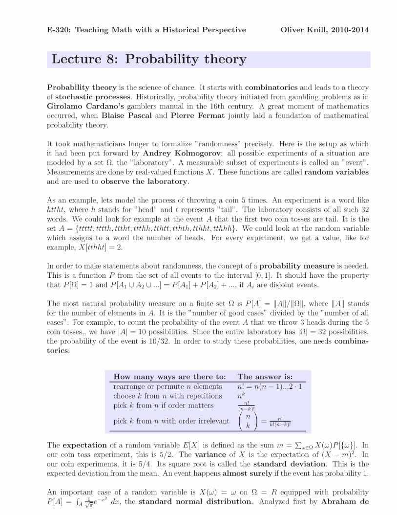
How many ways are there to: The answer is:

rearrange or permute n elements n! = n(n− 1)...2 · 1choose k from n with repetitions nk

pick k from n if order matters n!(n−k)!

pick k from n with order irrelevant

(

nk

)

= n!k!(n−k)!

The expectation of a random variable E[X ] is defined as the sum m =∑

ω∈Ω X(ω)P [ω]. Inour coin toss experiment, this is 5/2. The variance of X is the expectation of (X − m)2. Inour coin experiments, it is 5/4. Its square root is called the standard deviation. This is theexpected deviation from the mean. An event happens almost surely if the event has probability 1.

An important case of a random variable is X(ω) = ω on Ω = R equipped with probabilityP [A] =

∫

A

1√πe−x2

dx, the standard normal distribution. Analyzed first by Abraham de

Moivre in 1733, it was studied by Carl Friedrich Gauss in 1807 and therefore also calledGaussian distribution.

Two random variables X, Y are called decorrelated, if E[XY ] = E[X ] · E[Y ]. If for any func-tions f, g also f(X) and g(Y ) are decorrelated, then X, Y are called independent. Two randomvariables are said to have the same distribution, if for any a < b, the events a ≤ X ≤ b anda ≤ Y ≤ b are independent. If X, Y are decorrelated, then the relation Var[X ] + Var[Y ] =Var[X + Y ] holds which is just Pythagoras theorem, because decorrelated can be understoodgeometrically: X − E[X ] and Y − E[Y ] are orthogonal. A common problem is to study the sumof independent random variables Xn with identical distribution. One abbreviates this IID. Hereare the three most important theorems which we formulate in the case, whee all random variablesare assumed to have expectatation 0 and standard deviation 1. Let Sn = X1 + ... + Xn be then’th sum of the IID random variables. It is also called a random walk.

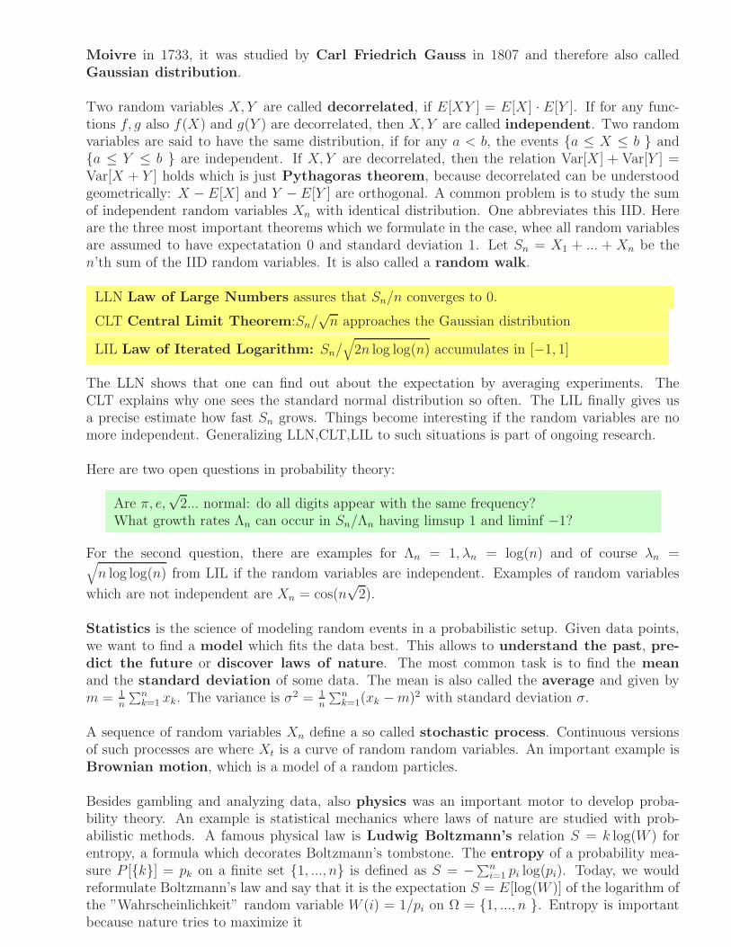
LLN Law of Large Numbers assures that Sn/n converges to 0.

CLT Central Limit Theorem:Sn/√n approaches the Gaussian distribution

LIL Law of Iterated Logarithm: Sn/√

2n log log(n) accumulates in [−1, 1]

The LLN shows that one can find out about the expectation by averaging experiments. TheCLT explains why one sees the standard normal distribution so often. The LIL finally gives usa precise estimate how fast Sn grows. Things become interesting if the random variables are nomore independent. Generalizing LLN,CLT,LIL to such situations is part of ongoing research.

Here are two open questions in probability theory:

Are π, e,√2... normal: do all digits appear with the same frequency?

What growth rates Λn can occur in Sn/Λn having limsup 1 and liminf −1?

For the second question, there are examples for Λn = 1, λn = log(n) and of course λn =√

n log log(n) from LIL if the random variables are independent. Examples of random variables

which are not independent are Xn = cos(n√2).

Statistics is the science of modeling random events in a probabilistic setup. Given data points,we want to find a model which fits the data best. This allows to understand the past, pre-dict the future or discover laws of nature. The most common task is to find the mean

and the standard deviation of some data. The mean is also called the average and given bym = 1

n

∑

n

k=1 xk. The variance is σ2 = 1n

∑

n

k=1(xk −m)2 with standard deviation σ.

A sequence of random variables Xn define a so called stochastic process. Continuous versionsof such processes are where Xt is a curve of random random variables. An important example isBrownian motion, which is a model of a random particles.

Besides gambling and analyzing data, also physics was an important motor to develop proba-bility theory. An example is statistical mechanics where laws of nature are studied with prob-abilistic methods. A famous physical law is Ludwig Boltzmann’s relation S = k log(W ) forentropy, a formula which decorates Boltzmann’s tombstone. The entropy of a probability mea-sure P [k] = pk on a finite set 1, ..., n is defined as S = −∑n

i=1 pi log(pi). Today, we wouldreformulate Boltzmann’s law and say that it is the expectation S = E[log(W )] of the logarithm ofthe ”Wahrscheinlichkeit” random variable W (i) = 1/pi on Ω = 1, ..., n . Entropy is importantbecause nature tries to maximize it

E-320: Teaching Math with a Historical Perspective Oliver Knill, 2014

Lecture 8: Probability theory

Petersburg Paradox

During class we look at the following vexing problem:

Problem We throw dices until tail appears. If ktimes head came first, we get 2

k dollars. What is afair fee to pay each time?

The paradox is that nobody would want to buy a 20 dollar entry fee. Mathematically, you winwith probability 2−k an amount of 2k leading to an infinite expectation.One solution is to look what happens if there is a limit K to the jackpot. The expected win isnow about log

2(K).

Martingale strategy

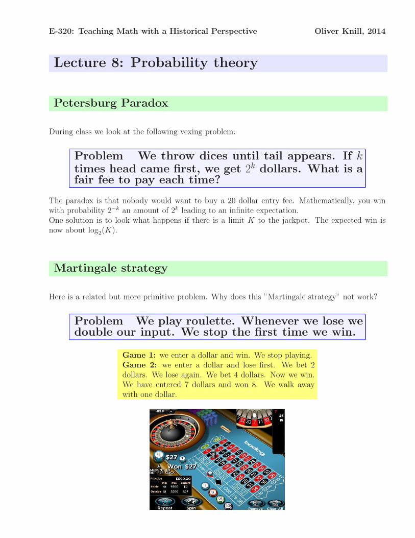
Here is a related but more primitive problem. Why does this ”Martingale strategy” not work?

Problem We play roulette. Whenever we lose wedouble our input. We stop the first time we win.

Game 1: we enter a dollar and win. We stop playing.Game 2: we enter a dollar and lose first. We bet 2dollars. We lose again. We bet 4 dollars. Now we win.We have entered 7 dollars and won 8. We walk awaywith one dollar.

Playing Blackjack

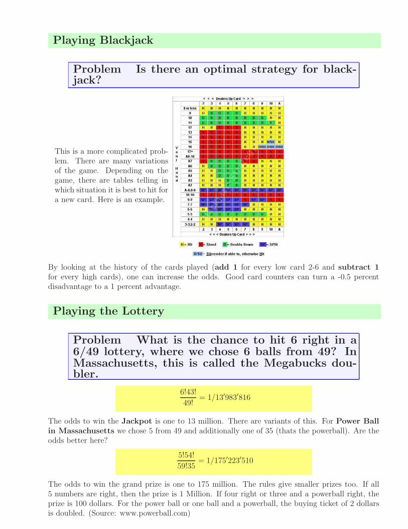
Problem Is there an optimal strategy for black-jack?

This is a more complicated prob-lem. There are many variationsof the game. Depending on thegame, there are tables telling inwhich situation it is best to hit fora new card. Here is an example.

By looking at the history of the cards played (add 1 for every low card 2-6 and subtract 1for every high cards), one can increase the odds. Good card counters can turn a -0.5 percentdisadvantage to a 1 percent advantage.

Playing the Lottery

Problem What is the chance to hit 6 right in a6/49 lottery, where we chose 6 balls from 49? InMassachusetts, this is called the Megabucks dou-bler.

6!43!

49!= 1/13′983′816

The odds to win the Jackpot is one to 13 million. There are variants of this. For Power Ballin Massachusetts we chose 5 from 49 and additionally one of 35 (thats the powerball). Are theodds better here?

5!54!

59!35= 1/175′223′510

The odds to win the grand prize is one to 175 million. The rules give smaller prizes too. If all5 numbers are right, then the prize is 1 Million. If four right or three and a powerball right, theprize is 100 dollars. For the power ball or one ball and a powerball, the buying ticket of 2 dollarsis doubled. (Source: www.powerball.com)

E-320: Teaching Math with a Historical Perspective Oliver Knill, 2010-2014

Lecture 9: Topology

Topology studies properties of geometric objects which do not change under continuous reversibledeformations. For a topologist, a coffee cup with 1 handle is the same as a doughnut. One candeform one into the other without punching any holes in it or ripping things apart. Similarly, aplate and a croissant are the same. But a croissant is not equivalent to a bagle. On a bagle, thereare closed curves which can not be deformed to a point. For a topologist the letters O and P are thesame but different from the letter B. The mathematical setup is beautiful: a topological space

is a set X with a set O of subsets of X containing both ∅ and X such that finite intersections andarbitrary unions in O are in O. Sets in O are called open sets and O is called a topology. Thecomplement of an open set is called closed. Examples of topologies are the trivial topology

O = ∅, X , where no open sets besides the empty set and X exist or the discrete topologyO = A ⊂ X ,, where every subset is open. But these are in general not interesting. Animportant example on the plane X is the collection O of sets U in the plane X for which everypoint is the center of a small disc still contained in U . A special class of topological spaces aremetric spaces, where a set X is equipped with a distance function d(x, y) = d(y, x) ≥ 0 whichsatisfies the triangle inequality d(x, y)+d(y, z) ≥ d(x, z) and for which d(x, y) = 0 if and only ifx = y. A set U in a metric space is open if to every x in U , there is a ball Br(x) = y|d(x, y) < r of positive radius r contained in U . Metric spaces are topological spaces but not all topologicalspaces are metric: the trivial topology for example is not in general. For doingcalculus on atopological space X , each point has a neighborhood called chart which is topologically equivalentto a disc in Euclidean space. Finitely many such neighborhoods covering X form an atlas of X . Ifthe charts are glued together with identification maps on the intersection one obtains a manifold.Two dimensional examples are the sphere, the torus, the projective plane or the Klein bottle.Topological spaces X, Y are called homeomorphic meaning ”topologically equivalent” if thereis an invertible map from X to Y which is also induces an invertible map on the correspondingtopologies. A basic task is to decide whether two spaces are equivalent in this sense or not. Thesurface of the coffee cup for example is equivalent in this sense to the surface of a doughnut butit is not equivalent to the surface of a sphere.Many properties of geometric spaces can be understood by replacing them with graphs forming askeleton of the space. A graph is a finite collection of vertices V together with a finite set of edgesE, where each edge connects two points in V . For example, the set V of cities in the US where theedges are pairs of cities connected by a street is a graph. The Konigsberg bridge problem wasa trigger puzzle for the study of graph theory. Polyhedra were an other start in graph theory.It study is losely related to the analysis of surfaces. The reason is that one can see polyhedraas discrete versions of surfaces. In computer graphics for example, surfaces are rendered as finitegraphs, using triangularizations.The Euler characteristic of a convex polyhedron is a remarkable topological invariant. It is

V − E + F = 2 , where V is the number of vertices, E the number of edges

and F the number of faces. This number is equal to 2 for connected polyhedra in which everyclosed loop can be pulled together to a point. This formula for the Euler characteristic is also calledEuler’s gem, a fact which comes with a rich history. Rene Descartes seems have stumbledupon it and written it down in a secret notebook. It was Leonard Euler in 1752 was the first toproved the formula for convex polyhedra. A convex polyhedron is called a platonic solid, if allvertices are on the unit sphere, all edges have the same length and all faces are congruent polygons.A theorem of Theaetetus states that there are only 5 platonic solids: [Proof: Assume the faces

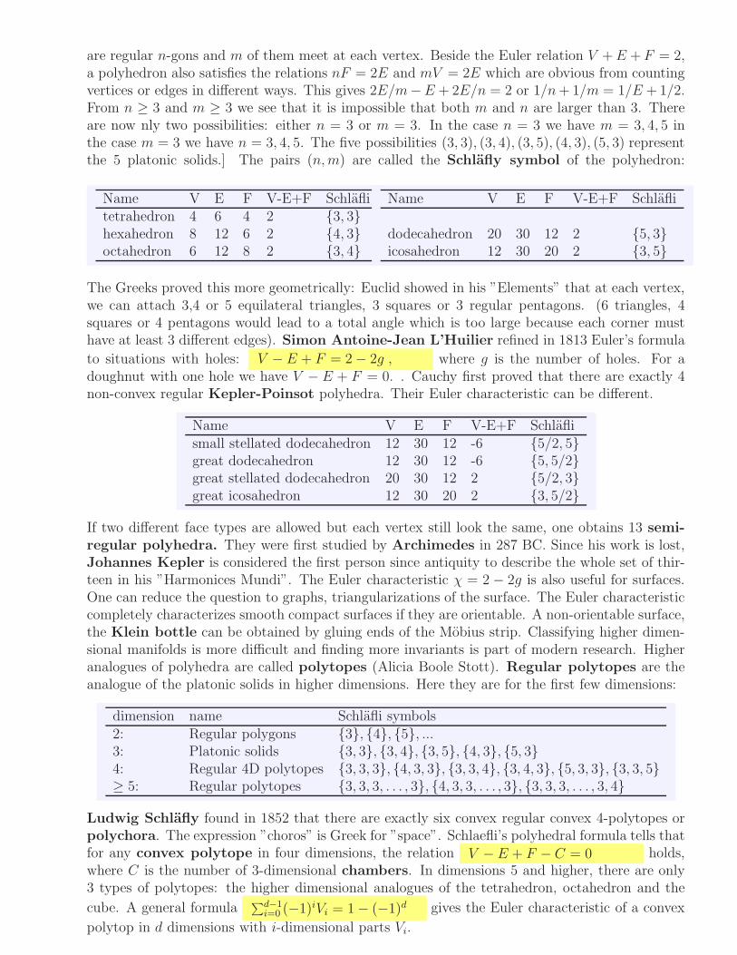
are regular n-gons and m of them meet at each vertex. Beside the Euler relation V +E + F = 2,a polyhedron also satisfies the relations nF = 2E and mV = 2E which are obvious from countingvertices or edges in different ways. This gives 2E/m−E + 2E/n = 2 or 1/n+ 1/m = 1/E +1/2.From n ≥ 3 and m ≥ 3 we see that it is impossible that both m and n are larger than 3. Thereare now nly two possibilities: either n = 3 or m = 3. In the case n = 3 we have m = 3, 4, 5 inthe case m = 3 we have n = 3, 4, 5. The five possibilities (3, 3), (3, 4), (3, 5), (4, 3), (5, 3) representthe 5 platonic solids.] The pairs (n,m) are called the Schlafly symbol of the polyhedron:

Name V E F V-E+F Schlaflitetrahedron 4 6 4 2 3, 3hexahedron 8 12 6 2 4, 3octahedron 6 12 8 2 3, 4

Name V E F V-E+F Schlafli

dodecahedron 20 30 12 2 5, 3icosahedron 12 30 20 2 3, 5

The Greeks proved this more geometrically: Euclid showed in his ”Elements” that at each vertex,we can attach 3,4 or 5 equilateral triangles, 3 squares or 3 regular pentagons. (6 triangles, 4squares or 4 pentagons would lead to a total angle which is too large because each corner musthave at least 3 different edges). Simon Antoine-Jean L’Huilier refined in 1813 Euler’s formula

to situations with holes: V − E + F = 2− 2g , where g is the number of holes. For adoughnut with one hole we have V − E + F = 0. . Cauchy first proved that there are exactly 4non-convex regular Kepler-Poinsot polyhedra. Their Euler characteristic can be different.

Name V E F V-E+F Schlaflismall stellated dodecahedron 12 30 12 -6 5/2, 5great dodecahedron 12 30 12 -6 5, 5/2great stellated dodecahedron 20 30 12 2 5/2, 3great icosahedron 12 30 20 2 3, 5/2

If two different face types are allowed but each vertex still look the same, one obtains 13 semi-

regular polyhedra. They were first studied by Archimedes in 287 BC. Since his work is lost,Johannes Kepler is considered the first person since antiquity to describe the whole set of thir-teen in his ”Harmonices Mundi”. The Euler characteristic χ = 2 − 2g is also useful for surfaces.One can reduce the question to graphs, triangularizations of the surface. The Euler characteristiccompletely characterizes smooth compact surfaces if they are orientable. A non-orientable surface,the Klein bottle can be obtained by gluing ends of the Mobius strip. Classifying higher dimen-sional manifolds is more difficult and finding more invariants is part of modern research. Higheranalogues of polyhedra are called polytopes (Alicia Boole Stott). Regular polytopes are theanalogue of the platonic solids in higher dimensions. Here they are for the first few dimensions:

dimension name Schlafli symbols2: Regular polygons 3, 4, 5, ...3: Platonic solids 3, 3, 3, 4, 3, 5, 4, 3, 5, 34: Regular 4D polytopes 3, 3, 3, 4, 3, 3, 3, 3, 4, 3, 4, 3, 5, 3, 3, 3, 3, 5≥ 5: Regular polytopes 3, 3, 3, . . . , 3, 4, 3, 3, . . . , 3, 3, 3, 3, . . . , 3, 4

Ludwig Schlafly found in 1852 that there are exactly six convex regular convex 4-polytopes orpolychora. The expression ”choros” is Greek for ”space”. Schlaefli’s polyhedral formula tells thatfor any convex polytope in four dimensions, the relation V − E + F − C = 0 holds,where C is the number of 3-dimensional chambers. In dimensions 5 and higher, there are only3 types of polytopes: the higher dimensional analogues of the tetrahedron, octahedron and the

cube. A general formula∑

d−1

i=0(−1)iVi = 1− (−1)d gives the Euler characteristic of a convex

polytop in d dimensions with i-dimensional parts Vi.

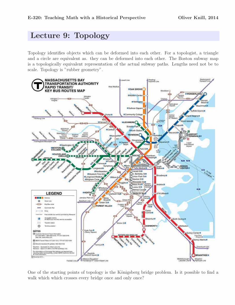
E-320: Teaching Math with a Historical Perspective Oliver Knill, 2014

Lecture 9: Topology

Topology identifies objects which can be deformed into each other. For a topologist, a triangleand a circle are equivalent as. they can be deformed into each other. The Boston subway mapis a topologically equivalent representation of the actual subway paths. Lengths need not be toscale. Topology is ”rubber geometry”.

One of the starting points of topology is the Konigsberg bridge problem. Is it possible to find awalk which which crosses every bridge once and only once?

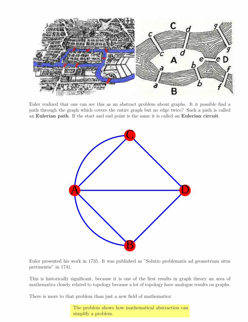
Euler realized that one can see this as an abstract problem about graphs. It it possible find apath through the graph which covers the entire graph but no edge twice? Such a path is calledan Eulerian path. If the start and end point is the same it is called an Eulerian circuit.

A D

C

BEuler presented his work in 1735. It was published as ”Solutio problematis ad geometriam situspertinentis” in 1741.

This is historically significant, because it is one of the first results in graph theory an area ofmathematics closely related to topology because a lot of topology have analogue results on graphs.

There is more to that problem than just a new field of mathematics:

The problem shows how mathematical abstraction cansimplify a problem.

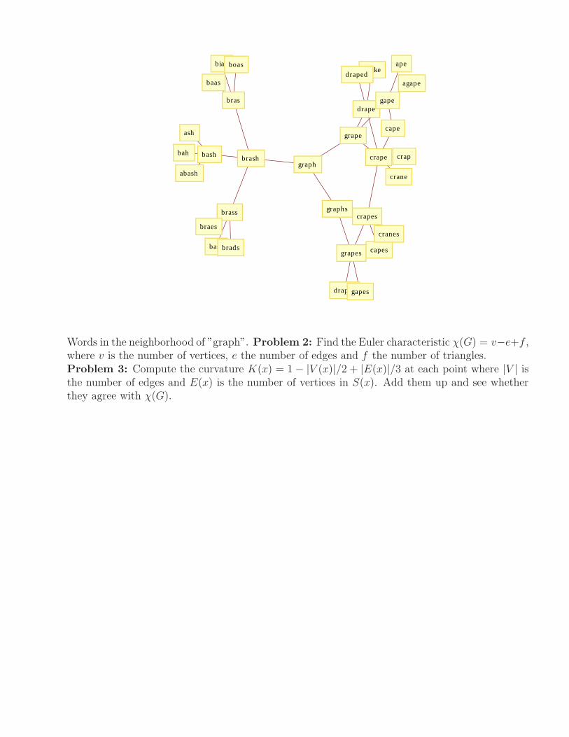
bash

abash

ash

bah

bras

baas

bias boas

brash

brass

bassbrads

braes

crape

cape

crane

crap

crapes

capes

cranes

drape

drakedraped

gape

agape

ape

grape

grapes

drapesgapes

graph

graphs

Words in the neighborhood of ”graph”. Problem 2: Find the Euler characteristic χ(G) = v−e+f ,where v is the number of vertices, e the number of edges and f the number of triangles.Problem 3: Compute the curvature K(x) = 1 − |V (x)|/2 + |E(x)|/3 at each point where |V | isthe number of edges and E(x) is the number of vertices in S(x). Add them up and see whetherthey agree with χ(G).

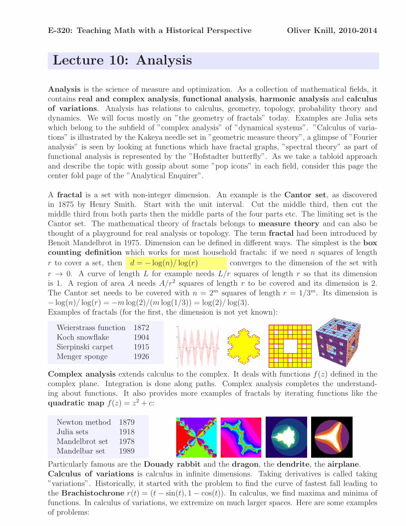
E-320: Teaching Math with a Historical Perspective Oliver Knill, 2010-2014

Lecture 10: Analysis

Analysis is the science of measure and optimization. As a collection of mathematical fields, itcontains real and complex analysis, functional analysis, harmonic analysis and calculus

of variations. Analysis has relations to calculus, geometry, topology, probability theory anddynamics. We will focus mostly on ”the geometry of fractals” today. Examples are Julia setswhich belong to the subfield of ”complex analysis” of ”dynamical systems”. ”Calculus of varia-tions” is illustrated by the Kakeya needle set in ”geometric measure theory”, a glimpse of ”Fourieranalysis” is seen by looking at functions which have fractal graphs, ”spectral theory” as part offunctional analysis is represented by the ”Hofstadter butterfly”. As we take a tabloid approachand describe the topic with gossip about some ”pop icons” in each field, consider this page thecenter fold page of the ”Analytical Enquirer”.

A fractal is a set with non-integer dimension. An example is the Cantor set, as discoveredin 1875 by Henry Smith. Start with the unit interval. Cut the middle third, then cut themiddle third from both parts then the middle parts of the four parts etc. The limiting set is theCantor set. The mathematical theory of fractals belongs to measure theory and can also bethought of a playground for real analysis or topology. The term fractal had been introduced byBenoit Mandelbrot in 1975. Dimension can be defined in different ways. The simplest is the box

counting definition which works for most household fractals: if we need n squares of length

r to cover a set, then d = − log(n)/ log(r) converges to the dimension of the set with

r → 0. A curve of length L for example needs L/r squares of length r so that its dimensionis 1. A region of area A needs A/r2 squares of length r to be covered and its dimension is 2.The Cantor set needs to be covered with n = 2m squares of length r = 1/3m. Its dimension is− log(n)/ log(r) = −m log(2)/(m log(1/3)) = log(2)/ log(3).Examples of fractals (for the first, the dimension is not yet known):

Weierstrass function 1872Koch snowflake 1904Sierpinski carpet 1915Menger sponge 1926

0.2 0.4 0.6 0.8 1.0

-0.5

0.5

1.0

Complex analysis extends calculus to the complex. It deals with functions f(z) defined in thecomplex plane. Integration is done along paths. Complex analysis completes the understand-ing about functions. It also provides more examples of fractals by iterating functions like thequadratic map f(z) = z2 + c:

Newton method 1879Julia sets 1918Mandelbrot set 1978Mandelbar set 1989

Particularly famous are the Douady rabbit and the dragon, the dendrite, the airplane.Calculus of variations is calculus in infinite dimensions. Taking derivatives is called taking”variations”. Historically, it started with the problem to find the curve of fastest fall leading tothe Brachistochrone r(t) = (t− sin(t), 1− cos(t)). In calculus, we find maxima and minima offunctions. In calculus of variations, we extremize on much larger spaces. Here are some examplesof problems:

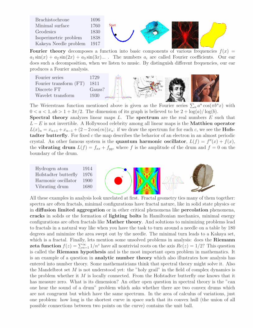
Brachistochrone 1696Minimal surface 1760Geodesics 1830Isoperimetric problem 1838Kakeya Needle problem 1917

Start

Fourier theory decomposes a function into basic components of various frequencies f(x) =a1 sin(x) + a2 sin(2x) + a3 sin(3x)... . The numbers ai are called Fourier coefficients. Our eardoes such a decomposition, when we listen to music. By distinguish different frequencies, our earproduces a Fourier analysis.

Fourier series 1729Fourier transform (FT) 1811Discrete FT Gauss?Wavelet transform 1930

-3 -2 -1 1 2 3

-0.2

0.2

0.4

0.6

0.8

1.0

The Weierstrass function mentioned above is given as the Fourier series∑

n an cos(πbnx) with

0 < a < 1, ab > 1 + 3π/2. The dimension of its graph is believed to be 2 + log(a)/ log(b).Spectral theory analyzes linear maps L. The spectrum are the real numbers E such thatL−E is not invertible. A Hollywood celebrity among all linear maps is the Matthieu operator

L(x)n = xn+1+xn−1+(2− 2 cos(cn))xn: if we draw the spectrum for for each c, we see the Hofs-

tadter butterfly. For fixed c the map describes the behavior of an electron in an almost periodiccrystal. An other famous system is the quantum harmonic oscillator, L(f) = f ′′(x) + f(x),the vibrating drum L(f) = fxx + fyy, where f is the amplitude of the drum and f = 0 on theboundary of the drum.

Hydrogen atom 1914Hofstadter butterfly 1976Harmonic oscillator 1900Vibrating drum 1680

+

-

All these examples in analysis look unrelated at first. Fractal geometry ties many of them together:spectra are often fractals, minimal configurations have fractal nature, like in solid state physics orin diffusion limited aggregation or in other critical phenomena like percolation phenomena,cracks in solids or the formation of lighting bolts In Hamiltonian mechanics, minimal energyconfigurations are often fractals like Mather theory. And solutions to minimizing problems leadto fractals in a natural way like when you have the task to turn around a needle on a table by 180degrees and minimize the area swept out by the needle. The minimal turn leads to a Kakaya set,which is a fractal. Finally, lets mention some unsolved problems in analysis: does the Riemann

zeta function f(z) =∑

∞

n=1 1/nz have all nontrivial roots on the axis Re(z) = 1/2? This question

is called the Riemann hypothesis and is the most important open problem in mathematics. Itis an example of a question in analytic number theory which also illustrates how analysis hasentered into number theory. Some mathematicians think that spectral theory might solve it. Alsothe Mandelbrot set M is not understood yet: the ”holy grail” in the field of complex dynamics isthe problem whether it M is locally connected. From the Hofstadter butterfly one knows that ithas measure zero. What is its dimension? An other open question in spectral theory is the ”canone hear the sound of a drum” problem which asks whether there are two convex drums whichare not congruent but which have the same spectrum. In the area of calculus of variations, justone problem: how long is the shortest curve in space such that its convex hull (the union of allpossible connections between two points on the curve) contains the unit ball.

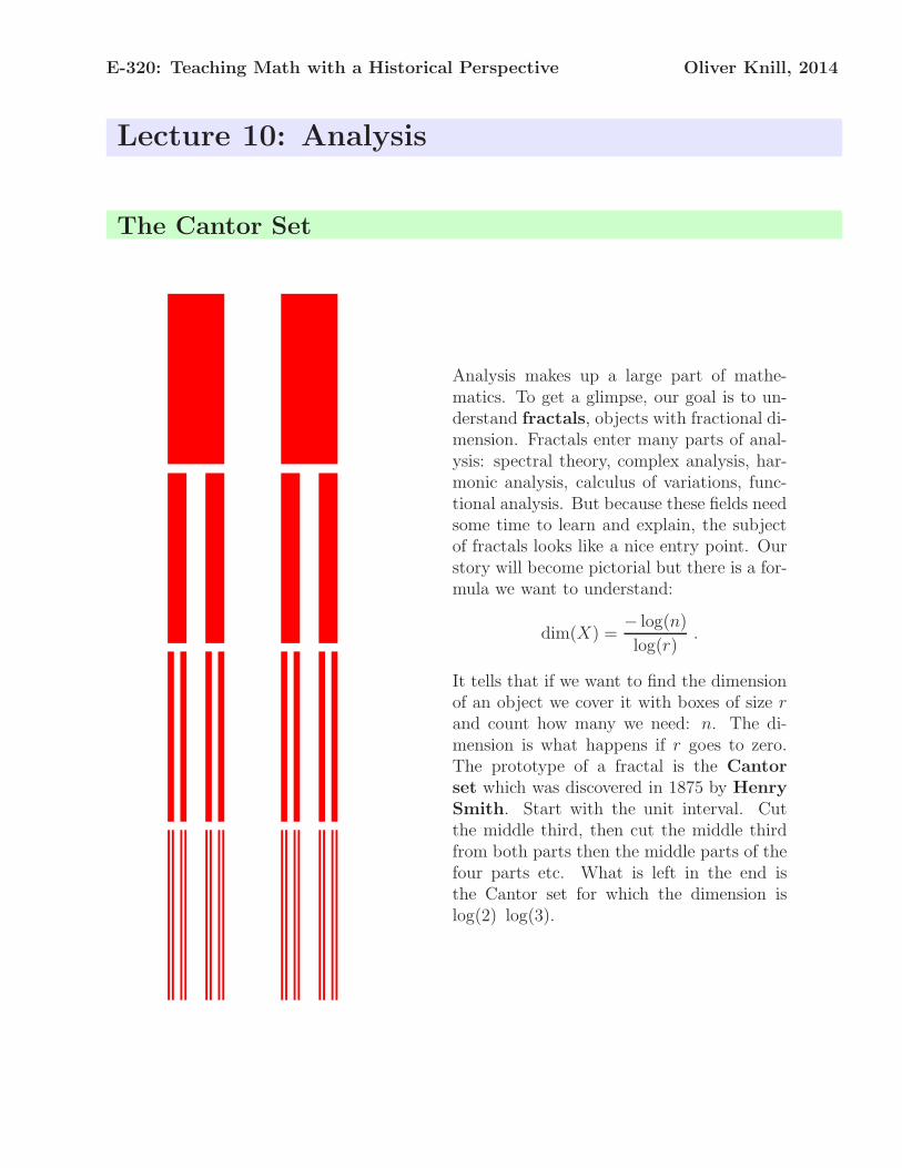
E-320: Teaching Math with a Historical Perspective Oliver Knill, 2014

Lecture 10: Analysis

The Cantor Set

Analysis makes up a large part of mathe-matics. To get a glimpse, our goal is to un-derstand fractals, objects with fractional di-mension. Fractals enter many parts of anal-ysis: spectral theory, complex analysis, har-monic analysis, calculus of variations, func-tional analysis. But because these fields needsome time to learn and explain, the subjectof fractals looks like a nice entry point. Ourstory will become pictorial but there is a for-mula we want to understand:

dim(X) =− log(n)

log(r).

It tells that if we want to find the dimensionof an object we cover it with boxes of size rand count how many we need: n. The di-mension is what happens if r goes to zero.The prototype of a fractal is the Cantor

set which was discovered in 1875 by Henry

Smith. Start with the unit interval. Cutthe middle third, then cut the middle thirdfrom both parts then the middle parts of thefour parts etc. What is left in the end isthe Cantor set for which the dimension islog(2) log(3).

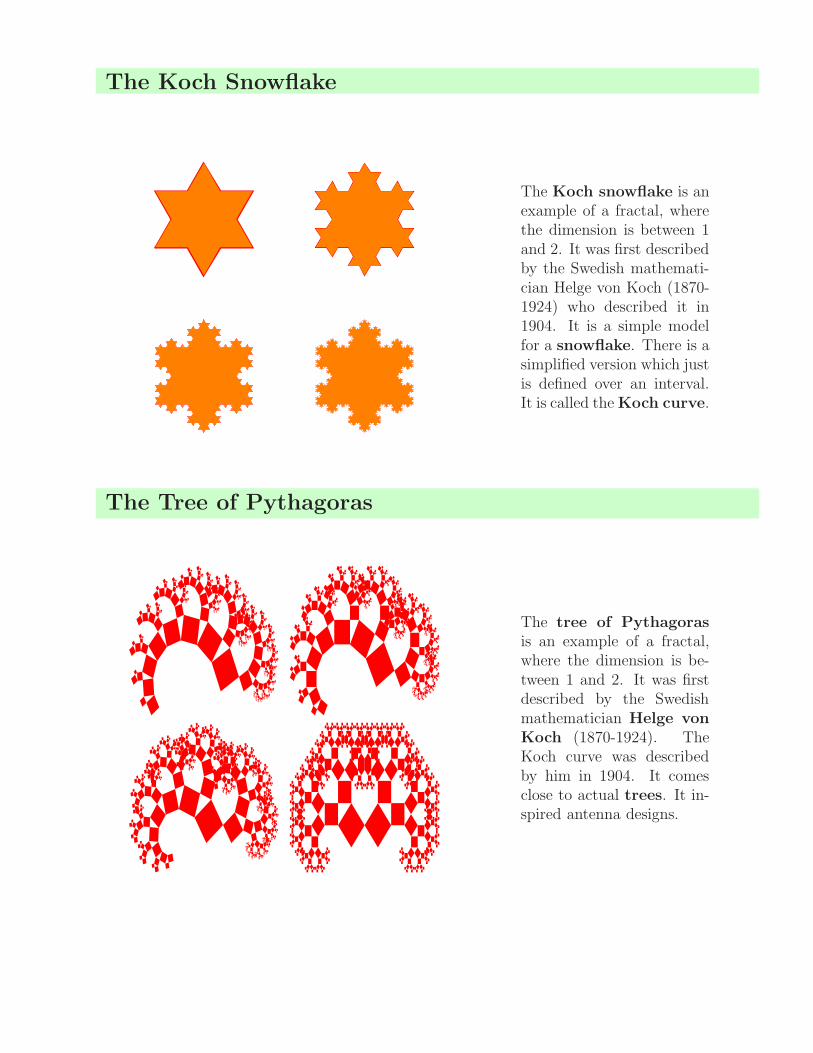
The Koch Snowflake

The Koch snowflake is anexample of a fractal, wherethe dimension is between 1and 2. It was first describedby the Swedish mathemati-cian Helge von Koch (1870-1924) who described it in1904. It is a simple modelfor a snowflake. There is asimplified version which justis defined over an interval.It is called theKoch curve.

The Tree of Pythagoras

The tree of Pythagoras

is an example of a fractal,where the dimension is be-tween 1 and 2. It was firstdescribed by the Swedishmathematician Helge von

Koch (1870-1924). TheKoch curve was describedby him in 1904. It comesclose to actual trees. It in-spired antenna designs.

The Sierpinski Carpet

The Sierpinski carpet isa fractal in the plane. Itsdimension is log(8)/ log(2).It was described byWaclav

Sierpinski in 1916.

The Menger Sponge

The Menger sponge is afractal in space. Its dimen-sion is between 2 and 3. Itwas first described by KarlMenger (1902-1985). Itsdimension is log(20)/ log(3)which is about 2.7.

The Mandelbrot set

We introduce complex numbers z = a+ ib and define complex multiplication

(a+ ib)(u + iv) = au− bv + (av + bu)i

Now look at the map T (z) = z2 + c where c is a fixed complex number. Start with z = i forexample, we get T (z) = i + c and T 2(z) = T (T (z)) = (i + c)2 + c etc. The Mandelbrot set

is the set of complex numbers c = a + ib for which T n(0) stays bounded. The filled in Julia

set Jcof c is the set of z such that T n(z) stays bounded. The Julia set is the boundary of that set.

For example, for c = 0, the map is T0(z) = z2. Since |zn| = |z|n we see that the disc |z| ≤ 1 isthe filled in Julia set for c = 0 and the unit circle |z| = 1 is the Julia set.

The following picture (Peitgen-Richter-Saupe) shows the Mandelbrot set in the c plane and a fewJulia sets. The circle is shown at the bottom.

A three dimensional version of the Mandelbrot set is called the Mandelbulb. It uses sphericalcoordinates which have been introduced by Euler.

E-320: Teaching Math with a Historical Perspective Oliver Knill, 2010

Lecture 11: Cryptography

Cryptography is the theory of codes. Two important aspects of the field are the encryption

rsp. decryption of information and error correction. Both are crucial in daily life. Whengetting access to a computer, viewing a bank statement or when taking money from the ATM,encryption algorithms are used. When phoning, surfing the web, accessing data on a computeror listening to music, error correction algorithms are used. Since our lives have become more andmore digital: music, movies, books, journals, finance, transportation, medicine, and communi-cation have become digital, we rely on strong error correction to avoid errors and encryption toassure things can not be tempered with. Without error correction, airplanes would crash: smallerrors in the memory of a computer would produce glitches in the navigation and control program.In a computer memory every hour a couple of bits are altered, for example by cosmic rays. Errorcorrection assures that this gets fixed. Without error correction music would sound like a 1920gramophone record. Without encryption, everybody could intrude electronic banks and transfermoney. Medical history shared with your doctor would all be public. Before the digital age, errorcorrection was assured by extremely redundant information storage. Writing a letter on a pieceof paper displaces billions of billions of molecules in ink. Now, changing any single bit could givea letter a different meaning. Before the digital age, information was kept in well guarded safeswhich were physically difficult to penetrate. Now, information is locked up in computers whichare connected to other computers. Vaults, money or voting ballots are secured by mathematicalalgorithms which assure that information can only be accessed by authorized users. Also lifeneeds error correction: information in the genome is stored in a genetic code, where a errorcorrection makes sure that life can survive. A cosmic ray hitting the skin changes the DNA ofa cell, but in general this is harmless. Only a larger amount of radiation can render cells cancerous.

How can an encryption algorithm be safe? One possibility is to invent a new method and keep itsecret. An other is to use a well known encryption method and rely on the difficulty of mathe-

matical computation tasks to assure that the method is safe. History has shown that the firstmethod is unreliable. Systems which rely on ”security through obfuscation” usually do not last.The reason is that it is tough to keep a method secret if the encryption tool is distributed. Reverseengineering of the method is often possible, for example using plain text attacks. Given a mapT , a third party can compute pairs x, T (x) and by choosing specific texts figure out what happens.

The Caesar cypher permutes the letters of the alphabet. We can for example replace every letterA with B, every letter B with C and so on until finally Z is replaced with A. The word ”Math-ematics” becomes so encrypted as ”Nbuifnbujdt”. Caesar would shift the letters by 3. The rightshift just discussed was used by his Nephew Augustus. Rot13 shifts by 13, and Atbash cypher

reflects the alphabet, switch A with Z, B with Y etc. The last two examples are involutive: en-cryption is decryption. More general cyphers are obtained by permuting the alphabet. Because of26! = 403291461126605635584000000 ∼ 1027 permutations, it appears first that a brute force at-tack is not possible. But Cesar cyphers can be cracked very quickly using statistical analysis. If weknow the frequency with which letters appear and match the frequency of a text we can figure outwhich letter was replaced with which. The Trithemius cypher prevents this simple analysis bychanging the permutation in each step. It is called a polyalphabetic substitution cypher. Insteadof a simple permutation, there are many permutations. After transcoding a letter, we also changethe key. Lets take a simple example. Rotate for the first letter the alphabet by 1, for the second

letter, the alphabet by 2, for the third letter, the alphabet by 3 etc. The word ”Mathematics” be-comes now ”Ncwljshbrmd”. Note that the second ”a” has been translated to something differentthan a. A frequency analysis is now more difficult. The Viginaire cypher adds even more com-plexity: instead of shifting the alphabet by 1, we can take a key like ”BCNZ”, then shift the firstletter by 1, the second letter by 3 the third letter by 13, the fourth letter by 25 the shift the 5thletter by 1 again. While this cypher remained unbroken for long, a more sophisticated frequencyanalysis which involves first finding the length of the key makes the cypher breakable. With theemergence of computers, even more sophisticated versions like the German enigma had no chance.

Diffie-Hellman key exchange allows Ana and Bob want to agree on a secret key over a publicchannel. The two palindromic friends agree on a prime number p and a base a. This informationcan be exchanged publically. Ana choses now a secret number x and sends X = ax modulo p

to Bob over the channel. Bob choses a secret number y and sends Y = ay modulo p to Ana.Ana can compute Y x and Bob can compute Xy but both are equal to axy. This number is theircommon secret. The key point is that eves dropper Eve, can not compute this number. The onlyinformation available to Eve are X and Y , as well as the base a and p. Eve knows that X = ax

but can not determine x. The key difficulty in this code is the discrete log problem: getting x

from ax modulo p is believed to be difficult for large p.The Rivest-Shamir-Adleman public key system uses a RSA public key (n, a) with aninteger n = pq and a < (p− 1)(q − 1), where p, q are prime. Also here, n and a are public. Onlythe factorization of n is kept secret. Ana publishes this pair. Bob who wants to email Ana amessage x, sends her y = xa mod n. Ana, who has computed b with ab = 1 mod (p−1)(q−1) canread the secrete email y because yb = xab = x(p−1)(q−1) = x modn. But Eve, has no chance becausethe only thing Eve knows is y and (n, a). It is believed that without the factorization of n, itis not possible to determine x. The message has been transmitted securely. The core difficulty isthat taking roots in the ring Zn = 0, . . . , n− 1 is difficult without knowing the factorizationof n. With a factorization, we can quickly take arbitrary roots. If we can take square roots, thenwe can also factor: assume we have a product n = pq and we know how to take square roots of 1.If x solves x2 = 1 mod n and x is different from 1, then x2 − 1 = (x− 1)(x+ 1) is zero modulo n.This means that p divides (x− 1) or (x+ 1). To find a factor, we can take the greatest commondivisor of n, x − 1. Take n = 77 for example. We are given the root 34 of 1. ( 342 = 1156 hasreminder 1 when divided by 34). The greatest common divisor of 34−1 and 77 is 11 is a factor of77. Similarly, the greatest common divisor of 34+ 1 and 77 is 7 divides 77. Finding roots moduloa composite number and factoring the number is equally difficult.

Cipher Used for Difficulty AttackCesar transmitting messages many permutations StatisticsViginere transmitting messages many permutations StatisticsEnigma transmitting messages no frequency analysis Plain textDiffie-Helleman agreeing on secret key discrete log mod p Unsafe primesRSA electronic commerce factoring integers Factoring

The simplest error correcting code uses 3 copies of the same information. A single error canbe corrected. With 3 watches for example, you know the time even if one of the watches fails.Cockpits of airplanes have three copies important instruments. But this basic error correctingcode is not efficient. It can correct single errors by tripling the size. Its efficiency is 33 percent.A cheap way to make it more efficient is to compress the data first and then make three copies.Data compression is a topic by itself. Here is a simple example, the dictionary compression.Take dictionary with 65′536 = 216 words for example. Every word can be encode by two bytes.Assuming an average word length of 6, we can encode every word with 2 bytes instead of 6. There

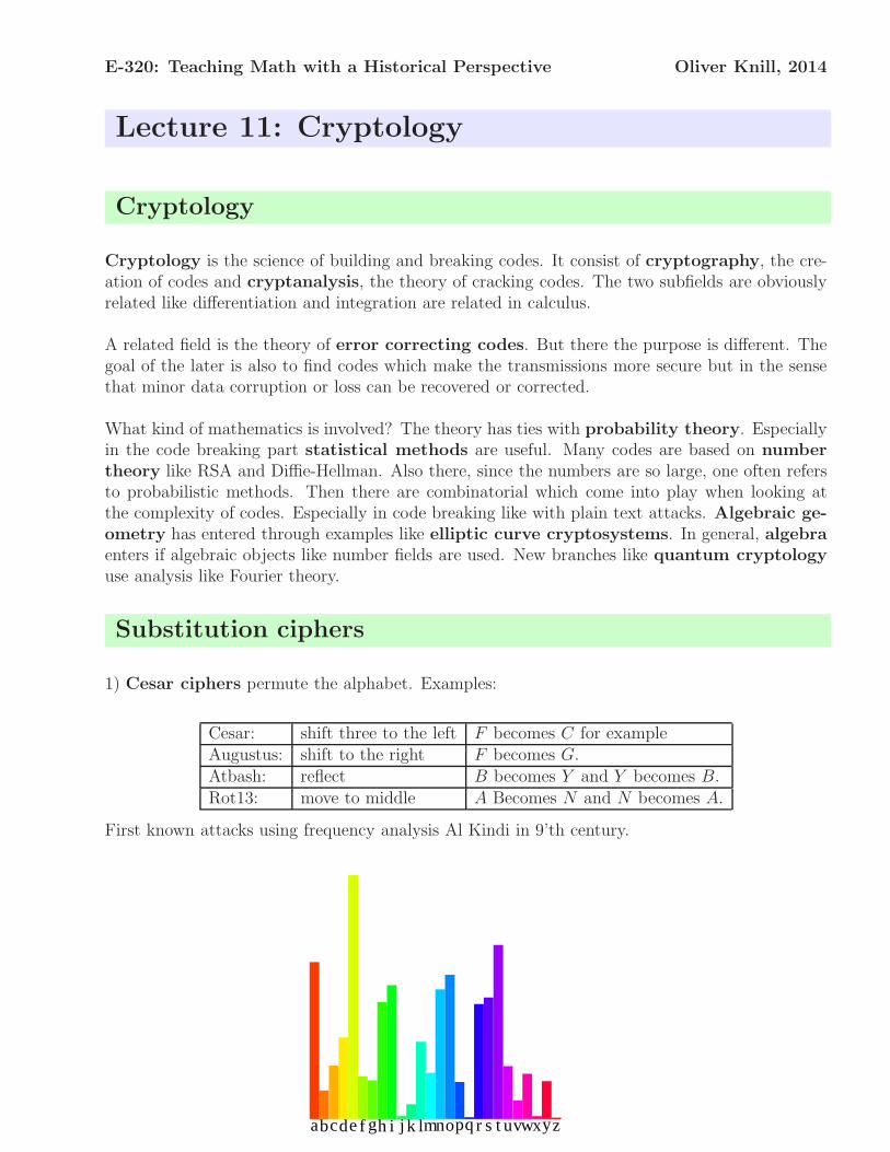
E-320: Teaching Math with a Historical Perspective Oliver Knill, 2014

Lecture 11: Cryptology

Cryptology

Cryptology is the science of building and breaking codes. It consist of cryptography, the cre-ation of codes and cryptanalysis, the theory of cracking codes. The two subfields are obviouslyrelated like differentiation and integration are related in calculus.

A related field is the theory of error correcting codes. But there the purpose is different. Thegoal of the later is also to find codes which make the transmissions more secure but in the sensethat minor data corruption or loss can be recovered or corrected.

What kind of mathematics is involved? The theory has ties with probability theory. Especiallyin the code breaking part statistical methods are useful. Many codes are based on number

theory like RSA and Diffie-Hellman. Also there, since the numbers are so large, one often refersto probabilistic methods. Then there are combinatorial which come into play when looking atthe complexity of codes. Especially in code breaking like with plain text attacks. Algebraic ge-

ometry has entered through examples like elliptic curve cryptosystems. In general, algebraenters if algebraic objects like number fields are used. New branches like quantum cryptology

use analysis like Fourier theory.

Substitution ciphers

1) Cesar ciphers permute the alphabet. Examples:

Cesar: shift three to the left F becomes C for exampleAugustus: shift to the right F becomes G.Atbash: reflect B becomes Y and Y becomes B.Rot13: move to middle A Becomes N and N becomes A.

First known attacks using frequency analysis Al Kindi in 9’th century.

abcde f gh i j k lmnopq r s t uvwxyz

2) Polyalaphabetic ciphers permute with different alphabets. Examples:

Alberti Random change of alphabet indicating switchTrithemius Deterministic change of alphabetViginere Using key telling which alphabet to useEnigma Using key and deterministic alphabet change overlapped with CesarHill Cipher Use matrices to permute

Block ciphers

Cut text into larger chunks and scramble them. Examples:

DES Data Encryption Standards 1973Triple DES Used for some electronic payments, 1998

Public Key Cyphers

Depends often on Number theoretical mathematical difficulties like factoring integers.

Diffie-Hellman Key exchange 1976 (1974 at GCHQ in England)RSA encryption 1978 (1973 at GCHQ in England)

The RSA method allows Ana to submit messages to Bob on a public channelwhich a third party Eve can not read.

Ana publishes a RSA pair: (n, a) of integers into the public. The factorization n = pq is secretand a < (p − 1)(q − 1) is such that there exists b with ab = 1 mod (p − 1)(q − 1). Bob sends asecrete message to Ana by transmitting

y = xa mod n .

Ana can read the email by computingyb mod n .

The key is public. Still, one can not read the messages unless a hard mathematical problem, thefactorization of n is solved.

Diffie Hellman method allows Ana and Bob to exchange keys on a publicchannel which a third party Eve can not read.

A prime p and primitive root a are given and public. A primitive root is a number for which ak

generates all numbers different from 0 modulo p. Its a number for which the ”log” exists.

Ana choses a secret number x and publishes u = ax mod p.Bob choses a secret number y and publishes v = ay mod p.Ana can compute vx = axy and Bob can compute vy = ayx (always modulo p) But Eve, the evesdropper can not get x, y from u, v.

E-320: Teaching Math with a Historical Perspective Oliver Knill, 2010-2014

Lecture 12: Dynamical systems

Dynamical systems theory is the science of time evolution. If time is continuous the evo-lution is defined by a differential equation x = f(x). If time is discrete then we look at theiteration of a map x → T (x).

The goal is to predict the future of the system when the present state is known. A differential

equation is an equation of the form d/dtx(t) = f(x(t)), where the unknown quantity is a pathx(t) in some “phase space”. We know the velocity d/dtx(t) = x(t) at all times and the initialconfiguration x(0)), we can to compute the trajectory x(t). What happens at a future time?Does x(t) stay in a bounded region or escape to infinity? Which areas of the phase space arevisited and how often? Can we reach a certain part of the space when starting at a given pointand if yes, when. An example of such a question is to predict, whether an asteroid located at a spe-cific location will hit the earth or not. An other example is to predict the weather of the next week.

An examples of a dynamical systems in one dimension is the differential equation

x′(t) = x(t)(2− x(t)), x(0) = 1

It is called the logistic system and describes population growth. This system has the solutionx(t) = 2et/(1 + e2t) as you can see by computing the left and right hand side.

A map is a rule which assigns to a quantity x(t) a new quantity x(t + 1) = T (x(t)). The statex(t) of the system determines the situation x(t + 1) at time t + 1. An example is is the Ulam

map T (x) = 4x(1 − x) on the interval [0, 1]. This is an example, where we have no idea whathappens after a few hundred iterates even if we would know the initial position with the accuracyof the Planck scale.

Dynamical system theory has applications all fields of mathematics. It can be used to find rootsof equations like for

T (x) = x− f(x)/f ′(x) .

A system of number theoretical nature is the Collatz map

T (x) =x

2(evenx), 3x+ 1 else .

A system of geometric nature is the Pedal map which assigns to a triangle the pedal triangle.

About 100 years ago, Henry Poincare was able to deal with chaos of low dimensional systems.While statistical mechanics had formalized the evolution of large systems with probabilisticmethods already, the new insight was that simple systems like a three body problem or abilliard map can produce very complicated motion. It was Poincare who saw that even forsuch low dimensional and completely deterministic systems, random motion can emerge. Whilephysisists have dealt with chaos earlier by assuming it or artificially feeding it into equations likethe Boltzmann equation, the occurrence of stochastic motion in geodesic flows or billiards orrestricted three body problems was a surprise. These findings needed half a century to sink inand only with the emergence of computers in the 1960ies, the awakening happened. Icons like

wing of a butterfly can produce a tornado in Texas in a few weeks. The reason for this statementis that the complicated equations to simulate the weather reduce under extreme simplificationsand truncations to a simple differential equation x = σ(y − x), y = rx− y − xz, z = xy − bz, theLorenz system. For σ = 10, r = 28, b = 8/3, Ed Lorenz discovered in 1963 an interesting longtime behavior and an aperiodic ”attractor”. Ruelle-Takens called it a strange attractor. It is agreat moment in mathematics to realize that attractors of simple systems can become fractalson which the motion is chaotic. It suggests that such behavior is abundant. What is chaos? If adynamical system shows sensitive dependence on initial conditions, we talk about chaos.We will experiment with the two maps T (x) = 4x(1−x) and S(x) = 4x−4x2 which starting withthe same initial conditions will produce different outcomes after a couple of iterations.The sensitive dependence on initial conditions is measured by how fast the derivative dT n of then’th iterate grows. The exponential growth rate γ is called the Lyapunov exponent. A smallerror of the size h will be amplified to heγn after n iterates. In the case of the Logistic map withc = 4, the Lyapunov exponent is log(2) and an error of 10−16 is amplified to 2n · 10−16. For timen = 53 already the error is of the order 1. This explains the above experiment with the differentmaps. The maps T (x) and S(x) round differently on the level 10−16. After 53 iterations, theseinitial fluctuation errors have grown to a macroscopic size.Here is a famous open problem which has resisted many attempts to solve it: Show that the mapT (x, y) = (c sin(2πx) + 2x − y, x) with T n(x, y) = (fn(x, y), gn(x, y)) has sensitive dependenceon initial conditions on a set of positive area. More precisely, verify that for c > 2 and all n1

n

∫1

0

∫1

0log |∂xfn(x, y)| dxdy ≥ log( c

2). The left hand side converges to the average of the Lyapunov

exponents which is in this case also the entropy of the map. For some systems, one can computethe entropy. The logistic map with c = 4 for example, which is also called the Ulam map, hasentropy log(2). The cat map

T (x, y) = (2x+ y, x+ y) mod1

has entropy log |(√5 + 3)/2|. This is the logarithm of the larger eigenvalue of the matrix.

While questions about simple maps look artificial at first, the mechanisms prevail in other systems:in astronomy, when studying planetary motion or electrons in the van Allen belt, in mechanicswhen studying coupled penduli or nonlinear oscillators, in fluid dynamics when studying vortexmotion or turbulence, in geometry, when studying the evolution of light on a surface, the change ofweather or tsunamis in the ocean. Dynamical systems theory started historically with the problemto understand the motion of planets. Newton realized that this is governed by a differentialequation, the n-body problem

x′′

j (t) =n∑

i=1

cij(xi − xj)

|xi − xj |3,

where cij depends on the masses and the gravitational constant. If one body is the sun andno interaction of the planets is assumed and using the common center of gravity as the origin,this reduces to the Kepler problem x′′(t) = −Cx/|x|3, where planets move on ellipses, theradius vector sweeps equal area in each time and the period squared is proportional to the semi-major axes cubed. A great moment in astronomy was when Kepler derived these laws empirically.An other great moment in mathematics is Newton’s theoretically derivation from the differentialequations.

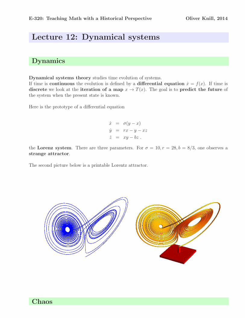
E-320: Teaching Math with a Historical Perspective Oliver Knill, 2014

Lecture 12: Dynamical systems

Dynamics

Dynamical systems theory studies time evolution of systems.If time is continuous the evolution is defined by a differential equation x = f(x). If time isdiscrete we look at the iteration of a map x → T (x). The goal is to predict the future ofthe system when the present state is known.

Here is the prototype of a differential equation

x = σ(y − x)

y = rx− y − xz

z = xy − bz .

the Lorenz system. There are three parameters. For σ = 10, r = 28, b = 8/3, one observes astrange attractor.

The second picture below is a printable Lorentz attractor.

Chaos

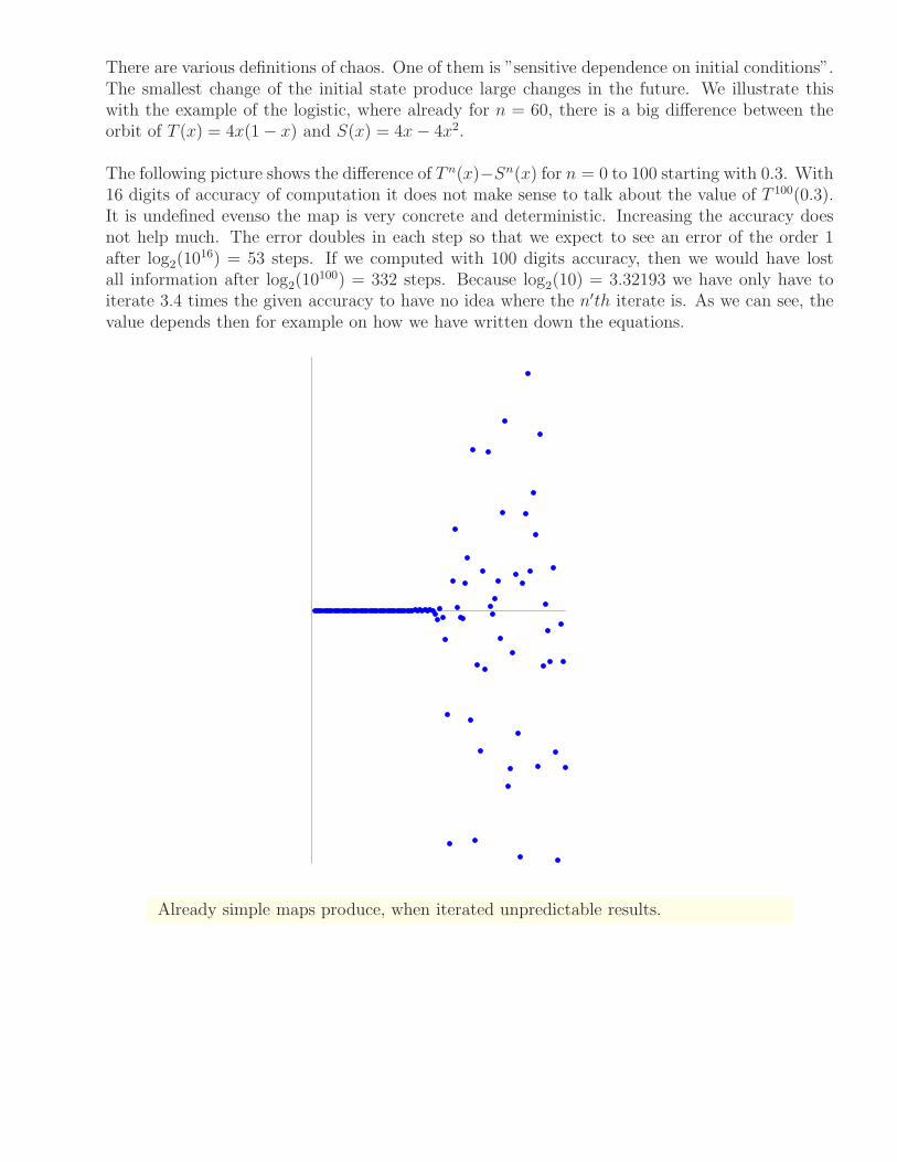
There are various definitions of chaos. One of them is ”sensitive dependence on initial conditions”.The smallest change of the initial state produce large changes in the future. We illustrate thiswith the example of the logistic, where already for n = 60, there is a big difference between theorbit of T (x) = 4x(1− x) and S(x) = 4x− 4x2.

The following picture shows the difference of T n(x)−Sn(x) for n = 0 to 100 starting with 0.3. With16 digits of accuracy of computation it does not make sense to talk about the value of T 100(0.3).It is undefined evenso the map is very concrete and deterministic. Increasing the accuracy doesnot help much. The error doubles in each step so that we expect to see an error of the order 1after log

2(1016) = 53 steps. If we computed with 100 digits accuracy, then we would have lost

all information after log2(10100) = 332 steps. Because log

2(10) = 3.32193 we have only have to

iterate 3.4 times the given accuracy to have no idea where the n′th iterate is. As we can see, thevalue depends then for example on how we have written down the equations.

Already simple maps produce, when iterated unpredictable results.

E-320: Teaching Math with a Historical Perspective Oliver Knill, 2010-2014

Lecture 13: Computing

Computing deals with algorithms and the praxis of programming. While the subject intersectswith computer science, information technology, the theory is by nature very mathematical. Butthere are new aspects: computers have opened the field of experimental mathematics andserve now as the laboratory for new mathematics. Computers are not only able to simulate

more and more of our physical world, they allow us to explore new worlds.A mathematician pioneering new grounds with computer experiments does similar work than anexperimental physicist. Computers have smeared the boundaries between physics and mathemat-ics. According to Borwein and Bailey, experimental mathematics consists of:

Gain insight and intuition.Find patterns and relationsDisplay mathematical principlesTest and falsify conjectures

Explore possible new resultsSuggest approaches for proofsAutomate lengthy hand derivationsConfirm already existing proofs

When using computers to prove things, reading and verifying the computer program is part ofthe proof. If Goldbach’s conjecture would be known to be true for all n > 1018, the conjectureshould be accepted because numerical verifications have been done until 2 · 1018 until today. Thefirst famous theorem proven with the help of a computer was the ”4 color theorem” in 1976.Here are some pointers in the history of computing:

2700BC Sumerian Abacus200BC Chinese Abacus150BC Astrolabe125BC Antikythera1300 Modern Abacus1400 Yupana1600 Slide rule1623 Schickard computer1642 Pascal Calculator1672 Leibniz multiplier1801 Punch cards1822 Difference Engine1876 Mechanical integrator

1935 Zuse 1 programmable1941 Zuse 31943 Harvard Mark I1944 Colossus1946 ENIAC1947 Transistor1948 Curta Gear Calculator1952 IBM 7011958 Integrated circuit1969 Arpanet1971 Microchip1972 Email1972 HP-35 calculator

1973 Windowed OS1975 Altair 88001976 Cray I1977 Apple II1981 Windows I1983 IBM PC1984 Macintosh1985 Atari1988 Next1989 HTTP1993 Webbrowser, PDA1998 Google2007 iPhone

We live in a time where technology explodes exponentially.Moore’s law from 1965 predicted thatsemiconductor technology doubles in capacity and overall performance every 2 years. This hashappened since. Some futurologists like Ray Kurzweil conclude from this technological singularityin which artificial intelligence might take over. Lets move to safer ground and discuss an importantconcept of computing, the question how to decide whether a computation is ”easy” or ”hard”. In1937, Alan Turing introduced the idea of a Turing machine, a theoretical model of a computerwhich allows to quantify complexity. It has finitely many states S = s1, ..., sn, h and works onan tape of 0−1 sequences. The state h is the ”halt” state. If it is reached, the machine stops. Themachine has rules which tells what it does if it is in state s and reads a letter a. Depending on s

and a, it writes 1 or 0 or moves the tape to the left or right and moves into a new state. Turingshowed that anything we know to compute today can be computed with Turing machines. For any

known machine, there is a polynomial p so that a computation done in k steps with that computercan be done in p(k) steps on a Turing machine. What can actually be computed? Church’s thesisof 1934 states that everything which can be computed can be computed with Turing machines.Similarly as in mathematics itself, there are limitations of computing. Turing’s setup allowed himto enumerate all possible Turing machine and use them as input of an other machine. Denote byTM the set of all pairs (T, x), where T is a Turing machine and x is a finite input. Let H ⊂ TM

denote the set of Turing machines (T, x) which halt with the tape x as input. Turing looked atthe decision problem: is there a machine which decides whether a given machine (T, x) is in H ornot. An ingenious Diagonal argument of Turing shows that the answer is ”no”. [Proof: assumethere is a machine HALT which returns from the input (T, x) the output HALT(T, x) = true, ifT halts with the input x and otherwise returns HALT(T, x) = false. Turing constructs a Turingmachine DIAGONAL, which does the following:

1) Read x. 2) Define Stop=HALT(x,x) 3) While Stop=True repeat Stop:=True; 4) Stop

Now, DIAGONAL is either in H or not. If DIAGONAL is in H, then the variable Stop is truewhich means that the machine DIAGONAL runs for ever and DIAGONAL is not in H. But ifDIAGONAL is not in H, then the variable Stop is false which means that the loop 3) is neverentered and the machine stops. The machine is in H.]Lets go back to the problem of distinguishing ”easy” and ”hard” problems: One calls P theclass of decision problems that are solvable in polynomial time and NP the class of decisionproblems which can efficiently be tested if the solution is given. These categories do not dependon the computing model used. The question ”N=NP?” is the most important open problem intheoretical computer science. It is one of the seven millenium problems and it is widely believedthat P 6= NP . If a problem is such that every other NP problem can be reduced to it, it is calledNP-complete. Popular games like Minesweeper or Tetris are NP-complete. If P 6= NP , thenthere is no efficient algorithm to beat the game. The intersection of NP-hard and NP is the classof NP-complete problems. An example of an NP-complete problem is the balanced number

partitioning problem: given n positive integers, divide them into two subsets A,B, so that thesum in A and the sum in B are as close as possible. A first shot: chose the largest remainingnumber and distribute it to alternatively to the two sets.We all feel that it is harder to find a solution to a problem rather than to verify a solution.If N 6= NP there are one way functions, functions which are easy to compute but hard to verify.For some important problems, we do not even know whether they are in NP. Here are two examples:1) the integer factoring problem: given n find the factors 2) the merit factor problem:minimize

∑nk=−n c

2k, where ck =

∑n−kj=0 ajaj+k An efficient algorithm for the first one would have

enormous consequences for ou modern lives.Finally, lets look at some mathematical problems in artificial intelligence AI:

problem solving playing games like chess, performing algorithms, solving puzzlespattern matching speech, music, image, face, handwriting, plagiarism detection, spamreconstruction tomography, city reconstruction, body scanningresearch computer assisted proofs, discovering theorems, verifying proofsdata mining knowledge acquisition, knowledge organization, learningtranslation language translation, porting applications to programming languagescreativity writing poems, jokes, novels, music pieces, painting, sculpturesimulation physics engines, evolution of bots, game development, aircraft designinverse problems earth quake location, oil depository, tomographyprediction weather prediction, climate change, warming, epidemics, supplies

We had started with basic human activities defining mathematical fields, we end the course withmathematical activities defining some aspects of computing. Our journey through math is over.

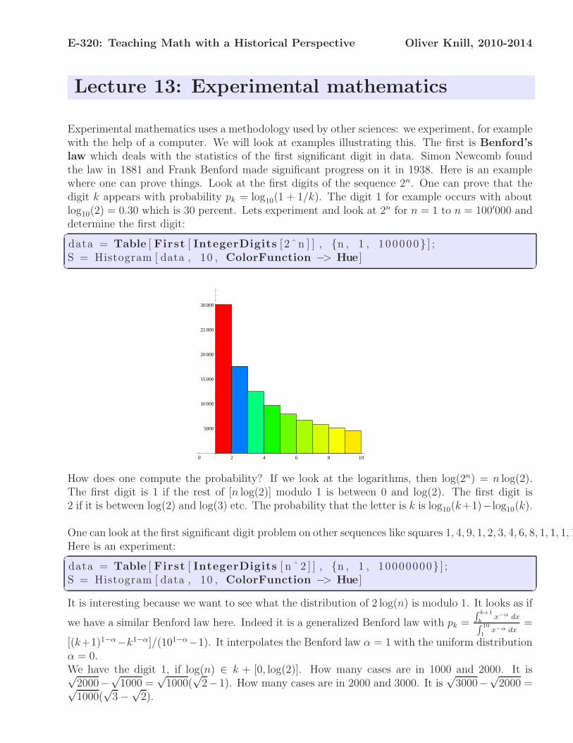
E-320: Teaching Math with a Historical Perspective Oliver Knill, 2010-2014

Lecture 13: Experimental mathematics

Experimental mathematics uses a methodology used by other sciences: we experiment, for examplewith the help of a computer. We will look at examples illustrating this. The first is Benford’s

law which deals with the statistics of the first significant digit in data. Simon Newcomb foundthe law in 1881 and Frank Benford made significant progress on it in 1938. Here is an examplewhere one can prove things. Look at the first digits of the sequence 2n. One can prove that thedigit k appears with probability pk = log

10(1 + 1/k). The digit 1 for example occurs with about

log10(2) = 0.30 which is 30 percent. Lets experiment and look at 2n for n = 1 to n = 100′000 and

determine the first digit:

data = Table [ First [ IntegerDigits [ 2 ˆn ] ] , n , 1 , 100000 ] ;S = Histogram [ data , 10 , ColorFunction −> Hue ]

0 2 4 6 8 10

5000

10 000

15 000

20 000

25 000

30 000

How does one compute the probability? If we look at the logarithms, then log(2n) = n log(2).The first digit is 1 if the rest of [n log(2)] modulo 1 is between 0 and log(2). The first digit is2 if it is between log(2) and log(3) etc. The probability that the letter is k is log

10(k+1)− log

10(k).

One can look at the first significant digit problem on other sequences like squares 1, 4, 9, 1, 2, 3, 4, 6, 8, 1, 1, 1, 1Here is an experiment:

data = Table [ First [ IntegerDigits [ n ˆ 2 ] ] , n , 1 , 10000000 ] ;S = Histogram [ data , 10 , ColorFunction −> Hue ]

It is interesting because we want to see what the distribution of 2 log(n) is modulo 1. It looks as if

we have a similar Benford law here. Indeed it is a generalized Benford law with pk =

∫k+1

kx−α

dx∫ 10

1x−α dx

=

[(k+1)1−α−k1−α]/(101−α−1). It interpolates the Benford law α = 1 with the uniform distributionα = 0.We have the digit 1, if log(n) ∈ k + [0, log(2)]. How many cases are in 1000 and 2000. It is√2000−

√1000 =

√1000(

√2−1). How many cases are in 2000 and 3000. It is

√3000−

√2000 =√

1000(√3−

√2).

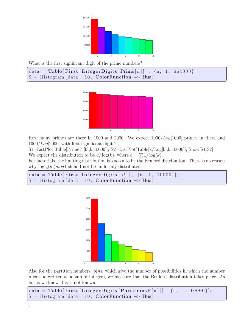
2 4 6 8 10

500 000

1.0´106

1.5´106

2.0´106

What is the first significant digit of the prime numbers?

data = Table [ First [ IntegerDigits [Prime [ n ] ] ] , n , 1 , 664000 ] ;S = Histogram [ data , 10 , ColorFunction −> Hue ]

2 4 6 8 10

20 000

40 000

60 000

80 000

How many primes are there in 1000 and 2000. We expect 1000/Log[1000] primes in there and1000/Log[2000] with first significant digit 2.S1=ListPlot[Table[PrimePi[k],k,10000]]; S2=ListPlot[Table[k/Log[k],k,10000]]; Show[S1,S2]We expect the distribution to be a/ log(k), where a =

∑1/ log(k).

For factorials, the limiting distribution is known to be the Benford distribution. There is no reasonwhy log

10(n!)mod1 should not be uniformly distributed.

data = Table [ First [ IntegerDigits [ n ! ] ] , n , 1 , 10000 ] ;S = Histogram [ data , 10 , ColorFunction −> Hue ]

0 2 4 6 8 10

500

1000

1500

2000

2500

3000

Also for the partition numbers, p(n), which give the number of possibilities in which the numbern can be written as a sum of integers, we measure that the Benford distribution takes place. Asfar as we know this is not known.

data = Table [ First [ IntegerDigits [PartitionsP [ n ] ] ] , n , 1 , 10000 ] ;S = Histogram [ data , 10 , ColorFunction −> Hue ]

s

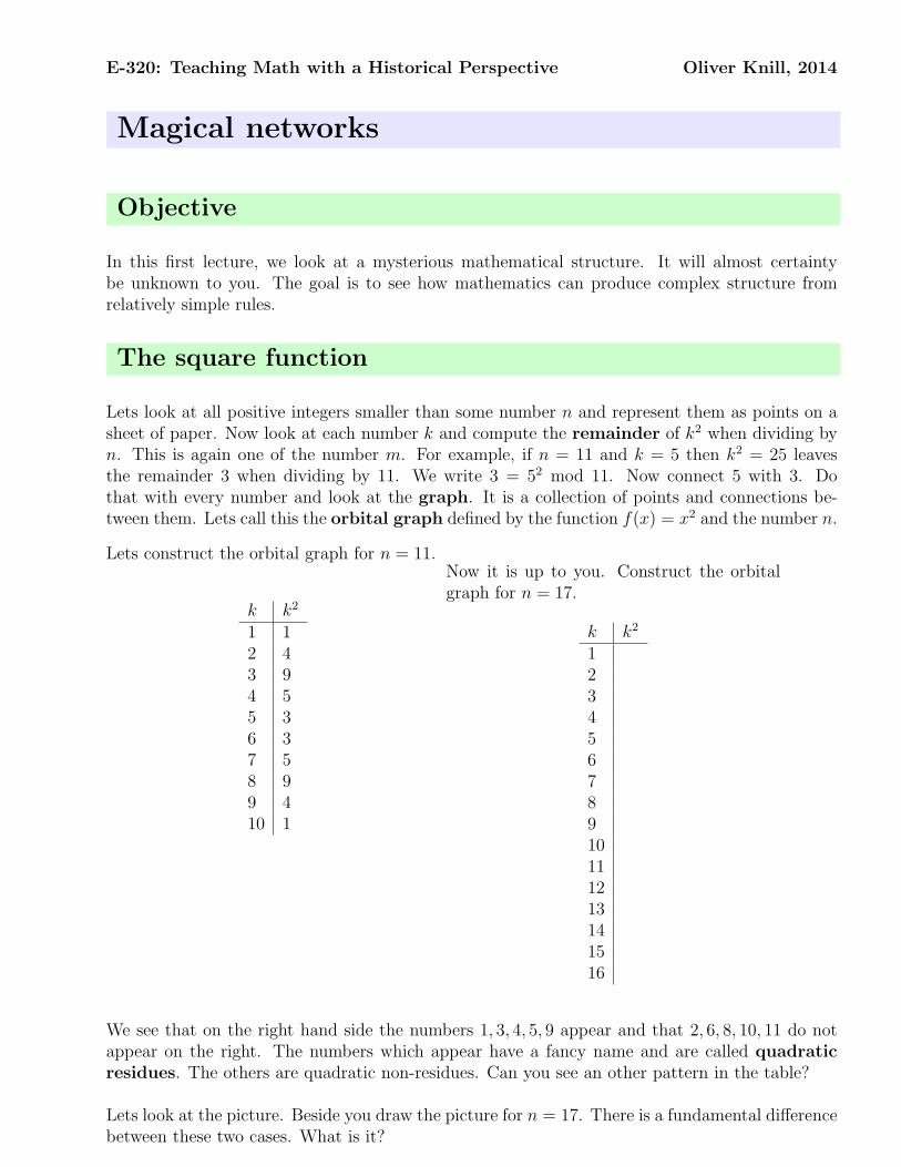
E-320: Teaching Math with a Historical Perspective Oliver Knill, 2014

Magical networks

Objective

In this first lecture, we look at a mysterious mathematical structure. It will almost certaintybe unknown to you. The goal is to see how mathematics can produce complex structure fromrelatively simple rules.

The square function

Lets look at all positive integers smaller than some number n and represent them as points on asheet of paper. Now look at each number k and compute the remainder of k2 when dividing byn. This is again one of the number m. For example, if n = 11 and k = 5 then k2 = 25 leavesthe remainder 3 when dividing by 11. We write 3 = 52 mod 11. Now connect 5 with 3. Dothat with every number and look at the graph. It is a collection of points and connections be-tween them. Lets call this the orbital graph defined by the function f(x) = x2 and the number n.

Lets construct the orbital graph for n = 11.

k k2

1 12 43 94 55 36 37 58 99 410 1

Now it is up to you. Construct the orbitalgraph for n = 17.

k k2

12345678910111213141516

We see that on the right hand side the numbers 1, 3, 4, 5, 9 appear and that 2, 6, 8, 10, 11 do notappear on the right. The numbers which appear have a fancy name and are called quadratic

residues. The others are quadratic non-residues. Can you see an other pattern in the table?

Lets look at the picture. Beside you draw the picture for n = 17. There is a fundamental differencebetween these two cases. What is it?

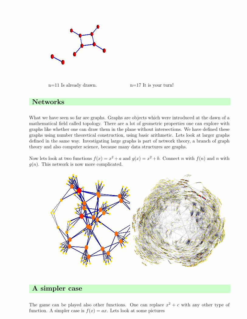
n=11 Is already drawn. n=17 It is your turn!

Networks

What we have seen so far are graphs. Graphs are objects which were introduced at the dawn of amathematical field called topology. There are a lot of geometric properties one can explore withgraphs like whether one can draw them in the plane without intersections. We have defined thesegraphs using number theoretical construction, using basic arithmetic. Lets look at larger graphsdefined in the same way. Investigating large graphs is part of network theory, a branch of graphtheory and also computer science, because many data structures are graphs.

Now lets look at two functions f(x) = x2 + a and g(x) = x2 + b. Connect n with f(n) and n withg(n). This network is now more complicated.

A simpler case

The game can be played also other functions. One can replace x2 + c with any other type offunction. A simpler case is f(x) = ax. Lets look at some pictures

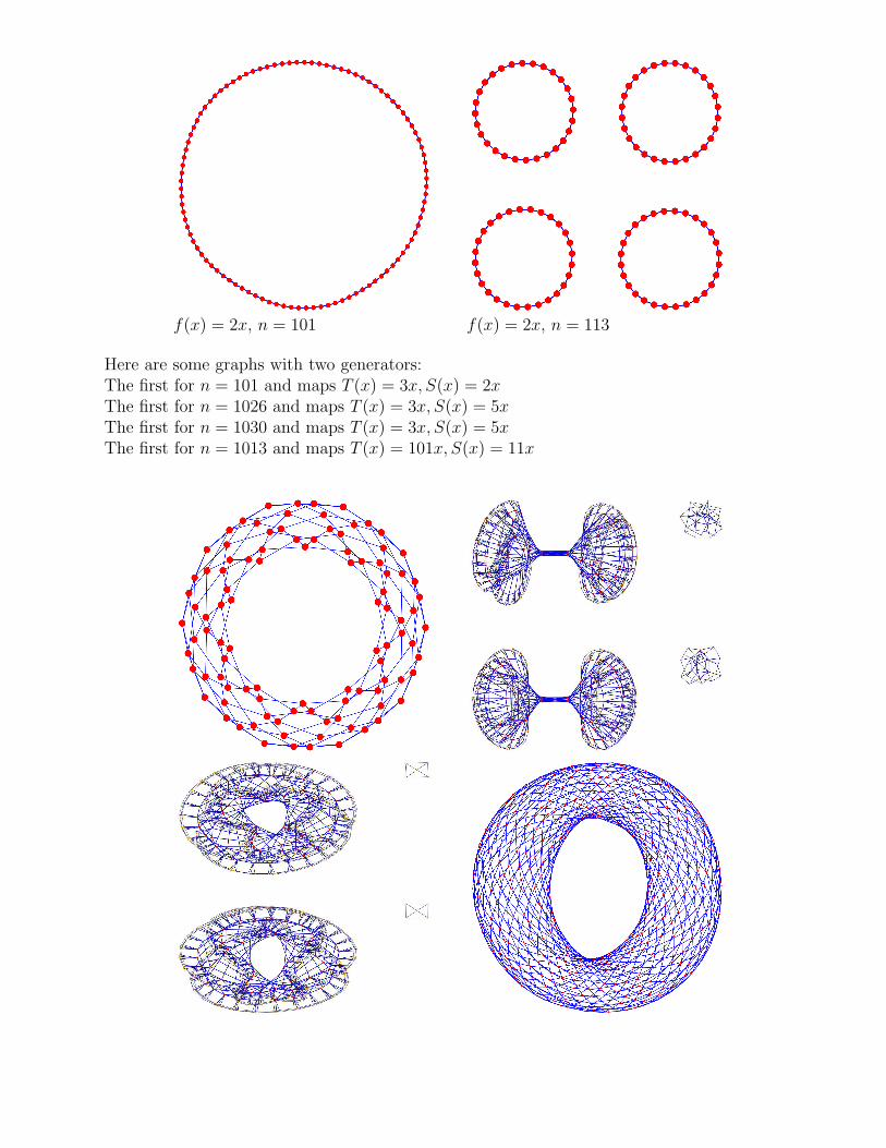
f(x) = 2x, n = 101 f(x) = 2x, n = 113

Here are some graphs with two generators:The first for n = 101 and maps T (x) = 3x, S(x) = 2xThe first for n = 1026 and maps T (x) = 3x, S(x) = 5xThe first for n = 1030 and maps T (x) = 3x, S(x) = 5xThe first for n = 1013 and maps T (x) = 101x, S(x) = 11x

More square cases

Here we see the square graphs for the first few primes. If you want to produce the graph yourself,you can check here whether you get the same thing.

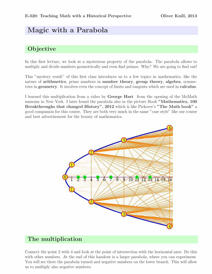
E-320: Teaching Math with a Historical Perspective Oliver Knill, 2013

Magic with a Parabola

Objective

In this first lecture, we look at a mysterious property of the parabola. The parabola allows tomultiply and divide numbers geometrically and even find primes. Why? We are going to find out!

This ”mystery result” of this first class introduces us to a few topics in mathematics, like thenature of arithmetics, prime numbers in number theory, group theory, algebra, symme-tries in geometry. It involves even the concept of limits and tangents which are used in calculus.

I learned this multiplication from a video by George Hart from the opening of the MoMathmuseum in New York. I later found the parabola also in the picture Book ”Mathematics, 100

Breakthroughs that changed History”, 2012 which is like Pickover’s ”The Math book” agood companion for this course. They are both very much in the same ”case style” like our courseand best advertisement for the beauty of mathematics.

The multiplication

Connect the point 2 with 4 and look at the point of intersection with the horizontal axes. Do thiswith other numbers. At the end of this handout is a larger parabola, where you can experiment.You will see there the parabola turned and negative numbers on the lower branch. This will allowus to multiply also negative numbers.

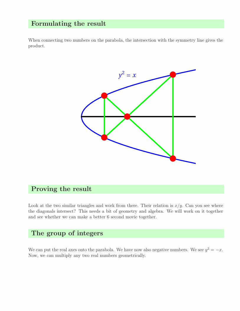
Formulating the result

When connecting two numbers on the parabola, the intersection with the symmetry line gives theproduct.

Proving the result

Look at the two similar triangles and work from there. Their relation is x/y. Can you see wherethe diagonals intersect? This needs a bit of geometry and algebra. We will work on it togetherand see whether we can make a better 6 second movie together.

The group of integers

We can put the real axes onto the parabola. We have now also negative numbers. We see y2 = −x.Now, we can multiply any two real numbers geometrically.

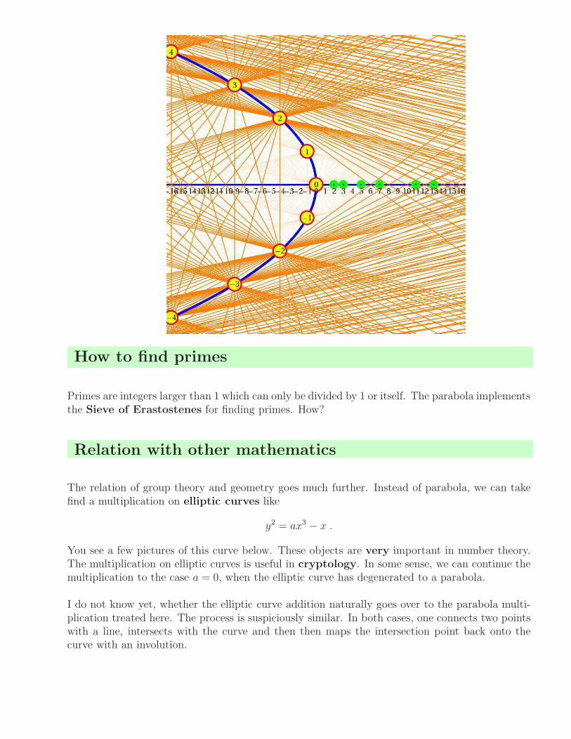
How to find primes

Primes are integers larger than 1 which can only be divided by 1 or itself. The parabola implementsthe Sieve of Erastostenes for finding primes. How?

Relation with other mathematics

The relation of group theory and geometry goes much further. Instead of parabola, we can takefind a multiplication on elliptic curves like

y2 = ax3 − x .

You see a few pictures of this curve below. These objects are very important in number theory.The multiplication on elliptic curves is useful in cryptology. In some sense, we can continue themultiplication to the case a = 0, when the elliptic curve has degenerated to a parabola.

I do not know yet, whether the elliptic curve addition naturally goes over to the parabola multi-plication treated here. The process is suspiciously similar. In both cases, one connects two pointswith a line, intersects with the curve and then then maps the intersection point back onto thecurve with an involution.

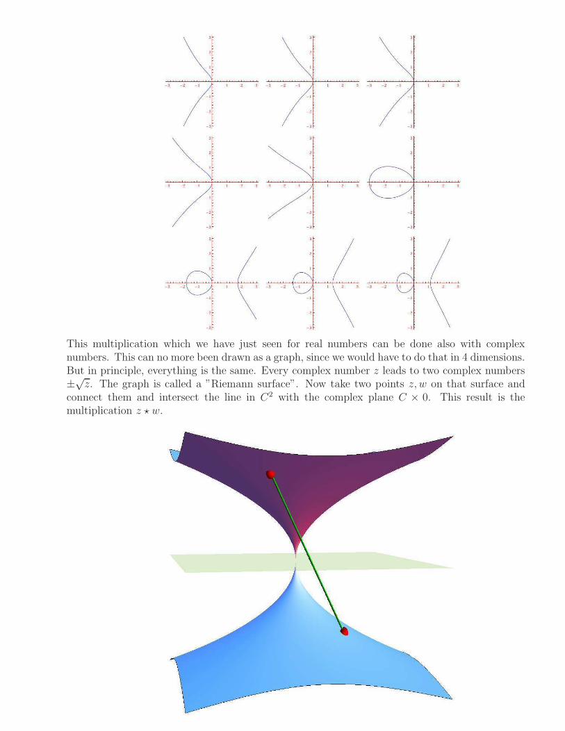
This multiplication which we have just seen for real numbers can be done also with complexnumbers. This can no more been drawn as a graph, since we would have to do that in 4 dimensions.But in principle, everything is the same. Every complex number z leads to two complex numbers±√z. The graph is called a ”Riemann surface”. Now take two points z, w on that surface and

connect them and intersect the line in C2 with the complex plane C × 0. This result is themultiplication z ⋆ w.

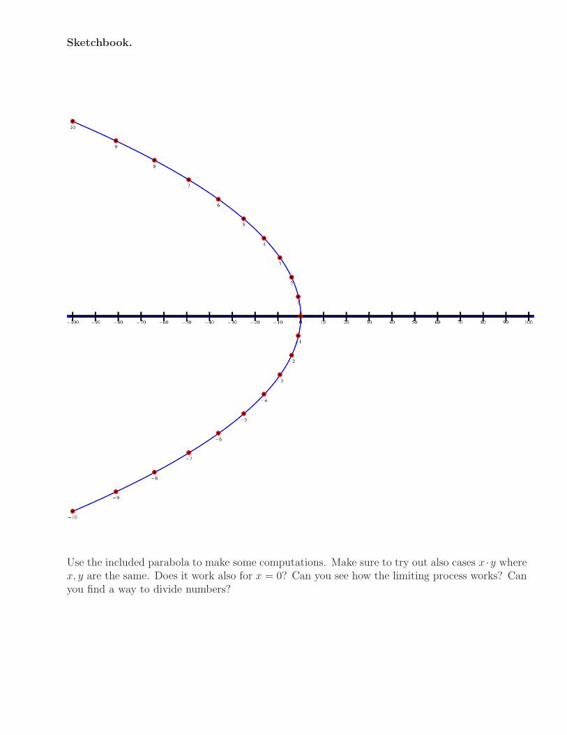
Sketchbook.

Use the included parabola to make some computations. Make sure to try out also cases x ·y wherex, y are the same. Does it work also for x = 0? Can you see how the limiting process works? Canyou find a way to divide numbers?

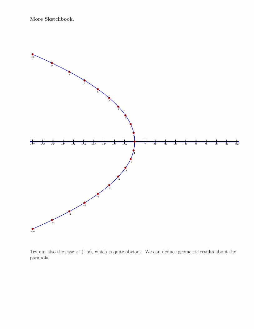
More Sketchbook.

Try out also the case x · (−x), which is quite obvious. We can deduce geometric results about theparabola.

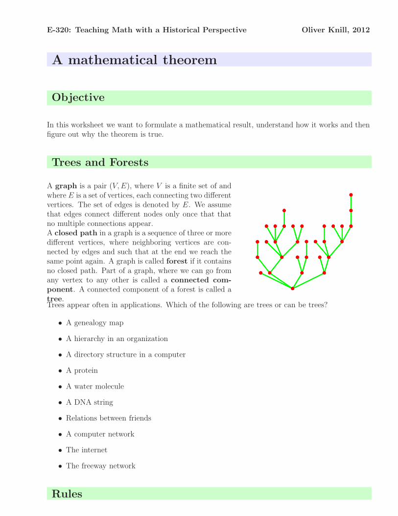
E-320: Teaching Math with a Historical Perspective Oliver Knill, 2012

A mathematical theorem

Objective

In this worksheet we want to formulate a mathematical result, understand how it works and thenfigure out why the theorem is true.

Trees and Forests

A graph is a pair (V,E), where V is a finite set of andwhere E is a set of vertices, each connecting two differentvertices. The set of edges is denoted by E. We assumethat edges connect different nodes only once that thatno multiple connections appear.A closed path in a graph is a sequence of three or moredifferent vertices, where neighboring vertices are con-nected by edges and such that at the end we reach thesame point again. A graph is called forest if it containsno closed path. Part of a graph, where we can go fromany vertex to any other is called a connected com-

ponent. A connected component of a forest is called atree.Trees appear often in applications. Which of the following are trees or can be trees?

• A genealogy map

• A hierarchy in an organization

• A directory structure in a computer

• A protein

• A water molecule

• A DNA string

• Relations between friends

• A computer network

• The internet

• The freeway network

Rules

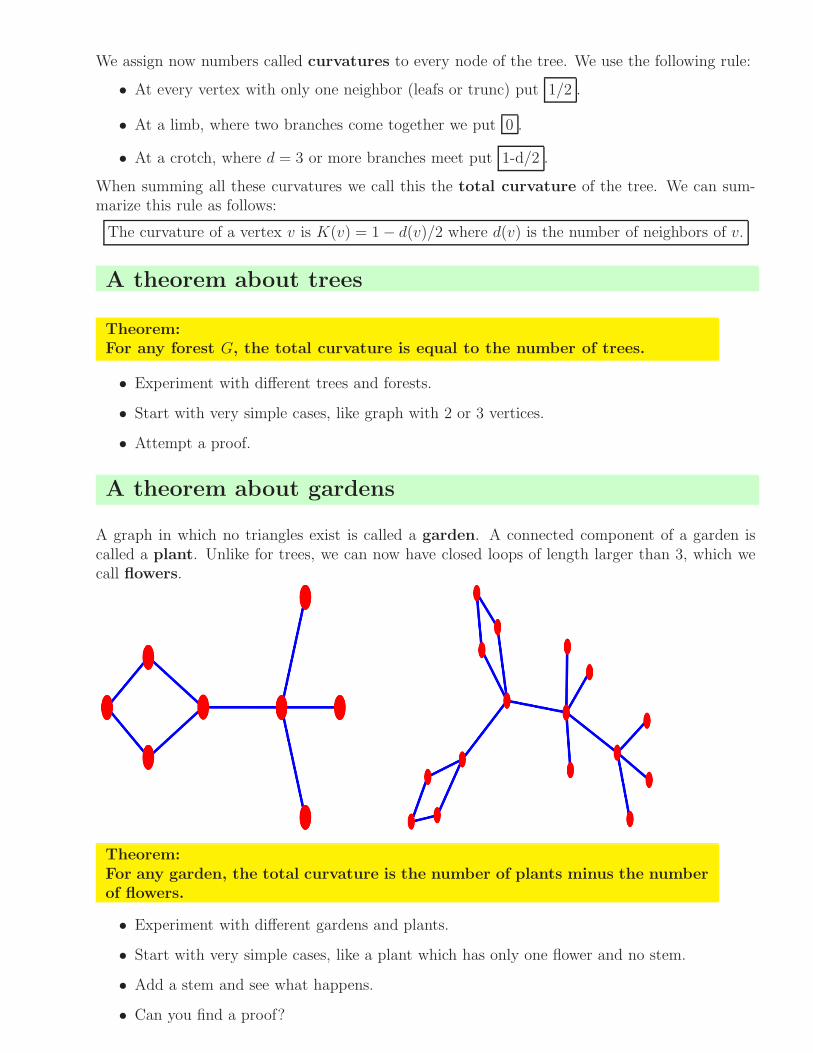
We assign now numbers called curvatures to every node of the tree. We use the following rule:

• At every vertex with only one neighbor (leafs or trunc) put 1/2 .

• At a limb, where two branches come together we put 0 .

• At a crotch, where d = 3 or more branches meet put 1-d/2 .

When summing all these curvatures we call this the total curvature of the tree. We can sum-marize this rule as follows:

The curvature of a vertex v is K(v) = 1− d(v)/2 where d(v) is the number of neighbors of v.

A theorem about trees

Theorem:

For any forest G, the total curvature is equal to the number of trees.

• Experiment with different trees and forests.

• Start with very simple cases, like graph with 2 or 3 vertices.

• Attempt a proof.

A theorem about gardens

A graph in which no triangles exist is called a garden. A connected component of a garden iscalled a plant. Unlike for trees, we can now have closed loops of length larger than 3, which wecall flowers.

Theorem:

For any garden, the total curvature is the number of plants minus the number

of flowers.

• Experiment with different gardens and plants.

• Start with very simple cases, like a plant which has only one flower and no stem.

• Add a stem and see what happens.

• Can you find a proof?

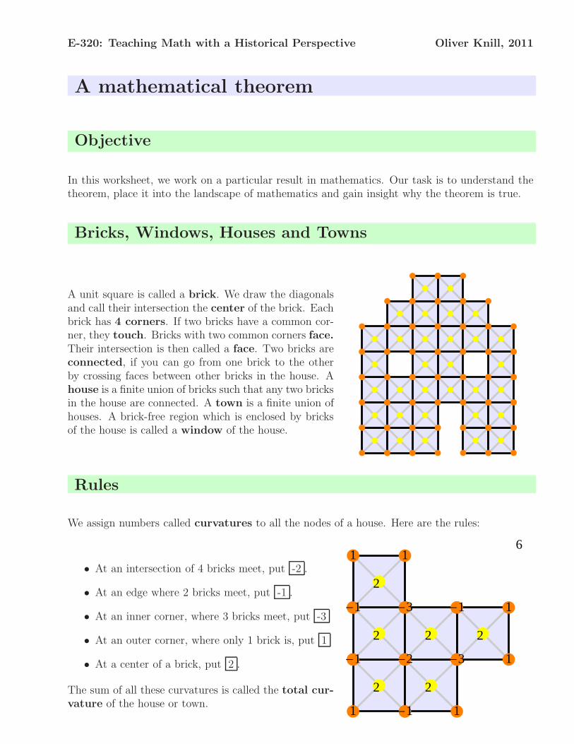
E-320: Teaching Math with a Historical Perspective Oliver Knill, 2011

A mathematical theorem

Objective

In this worksheet, we work on a particular result in mathematics. Our task is to understand thetheorem, place it into the landscape of mathematics and gain insight why the theorem is true.

Bricks, Windows, Houses and Towns

A unit square is called a brick. We draw the diagonalsand call their intersection the center of the brick. Eachbrick has 4 corners. If two bricks have a common cor-ner, they touch. Bricks with two common corners face.Their intersection is then called a face. Two bricks areconnected, if you can go from one brick to the otherby crossing faces between other bricks in the house. Ahouse is a finite union of bricks such that any two bricksin the house are connected. A town is a finite union ofhouses. A brick-free region which is enclosed by bricksof the house is called a window of the house.

Rules

We assign numbers called curvatures to all the nodes of a house. Here are the rules:

• At an intersection of 4 bricks meet, put -2 .

• At an edge where 2 bricks meet, put -1 .

• At an inner corner, where 3 bricks meet, put -3

• At an outer corner, where only 1 brick is, put 1

• At a center of a brick, put 2 .

The sum of all these curvatures is called the total cur-vature of the house or town.

2

2

2

2

2 2

1

-1

-1

1

-1

-2

-3

1

1

-3

-1

1

1

6

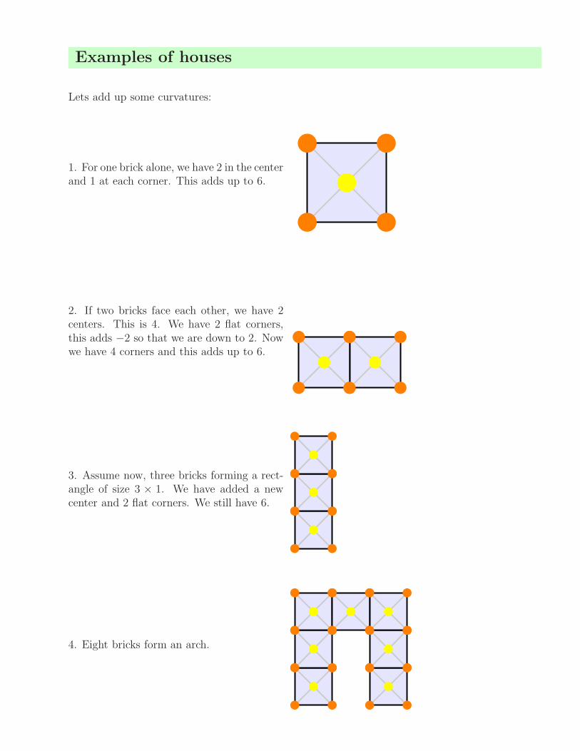
Examples of houses

Lets add up some curvatures:

1. For one brick alone, we have 2 in the centerand 1 at each corner. This adds up to 6.

2. If two bricks face each other, we have 2centers. This is 4. We have 2 flat corners,this adds −2 so that we are down to 2. Nowwe have 4 corners and this adds up to 6.

3. Assume now, three bricks forming a rect-angle of size 3 × 1. We have added a newcenter and 2 flat corners. We still have 6.

4. Eight bricks form an arch.

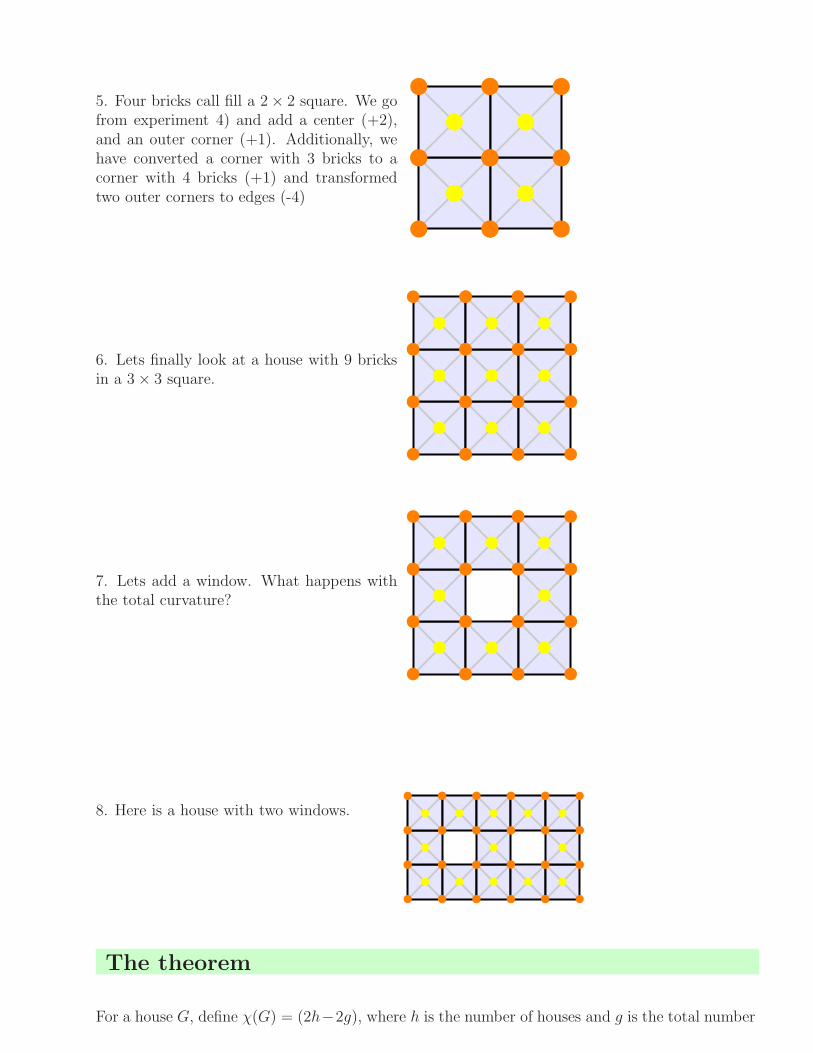
5. Four bricks call fill a 2× 2 square. We gofrom experiment 4) and add a center (+2),and an outer corner (+1). Additionally, wehave converted a corner with 3 bricks to acorner with 4 bricks (+1) and transformedtwo outer corners to edges (-4)

6. Lets finally look at a house with 9 bricksin a 3× 3 square.

7. Lets add a window. What happens withthe total curvature?

8. Here is a house with two windows.

The theorem

For a house G, define χ(G) = (2h−2g), where h is the number of houses and g is the total number

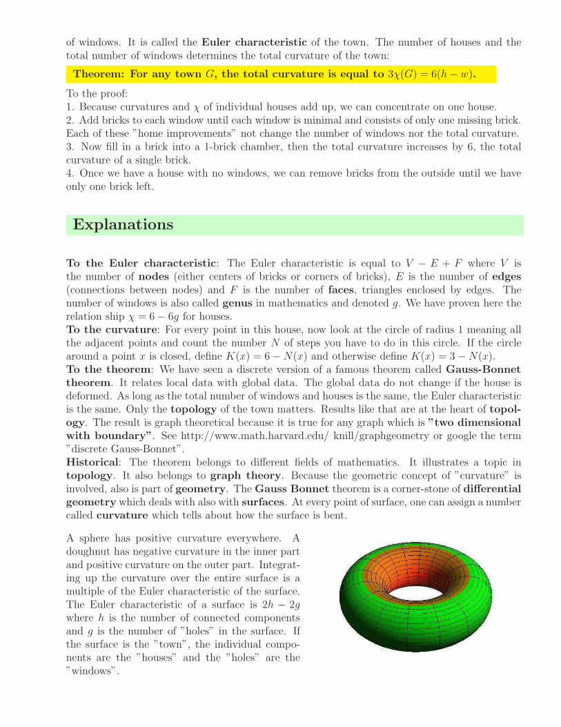
of windows. It is called the Euler characteristic of the town. The number of houses and thetotal number of windows determines the total curvature of the town:

Theorem: For any town G, the total curvature is equal to 3χ(G) = 6(h− w).

To the proof:1. Because curvatures and χ of individual houses add up, we can concentrate on one house.2. Add bricks to each window until each window is minimal and consists of only one missing brick.Each of these ”home improvements” not change the number of windows nor the total curvature.3. Now fill in a brick into a 1-brick chamber, then the total curvature increases by 6, the totalcurvature of a single brick.4. Once we have a house with no windows, we can remove bricks from the outside until we haveonly one brick left.

Explanations

To the Euler characteristic: The Euler characteristic is equal to V − E + F where V isthe number of nodes (either centers of bricks or corners of bricks), E is the number of edges(connections between nodes) and F is the number of faces, triangles enclosed by edges. Thenumber of windows is also called genus in mathematics and denoted g. We have proven here therelation ship χ = 6− 6g for houses.To the curvature: For every point in this house, now look at the circle of radius 1 meaning allthe adjacent points and count the number N of steps you have to do in this circle. If the circlearound a point x is closed, define K(x) = 6−N(x) and otherwise define K(x) = 3−N(x).To the theorem: We have seen a discrete version of a famous theorem called Gauss-Bonnet

theorem. It relates local data with global data. The global data do not change if the house isdeformed. As long as the total number of windows and houses is the same, the Euler characteristicis the same. Only the topology of the town matters. Results like that are at the heart of topol-ogy. The result is graph theoretical because it is true for any graph which is ”two dimensional

with boundary”. See http://www.math.harvard.edu/ knill/graphgeometry or google the term”discrete Gauss-Bonnet”.Historical: The theorem belongs to different fields of mathematics. It illustrates a topic intopology. It also belongs to graph theory. Because the geometric concept of ”curvature” isinvolved, also is part of geometry. The Gauss Bonnet theorem is a corner-stone of differentialgeometry which deals with also with surfaces. At every point of surface, one can assign a numbercalled curvature which tells about how the surface is bent.

A sphere has positive curvature everywhere. Adoughnut has negative curvature in the inner partand positive curvature on the outer part. Integrat-ing up the curvature over the entire surface is amultiple of the Euler characteristic of the surface.The Euler characteristic of a surface is 2h − 2gwhere h is the number of connected componentsand g is the number of ”holes” in the surface. Ifthe surface is the ”town”, the individual compo-nents are the ”houses” and the ”holes” are the”windows”.

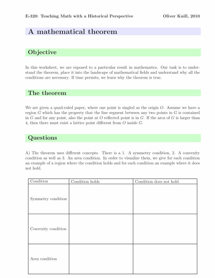
E-320: Teaching Math with a Historical Perspective Oliver Knill, 2010

A mathematical theorem

Objective

In this worksheet, we are exposed to a particular result in mathematics. Our task is to under-stand the theorem, place it into the landscape of mathematical fields and understand why all theconditions are necessary. If time permits, we learn why the theorem is true.

The theorem

We are given a quad-ruled paper, where one point is singled as the origin O. Assume we have aregion G which has the property that the line segment between any two points in G is containedin G and for any point, also the point at O reflected point is in G. If the area of G is larger than4, then there must exist a lattice point different from O inside G.

Questions

A) The theorem uses different concepts. There is a 1. A symmetry condition, 2. A convexitycondition as well as 3. An area condition. In order to visualize them, we give for each conditionan example of a region where the condition holds and for each condition an example where it doesnot hold.

Condition Condition holds Condition does not hold

Symmetry condition

Convexity condition

Area condition

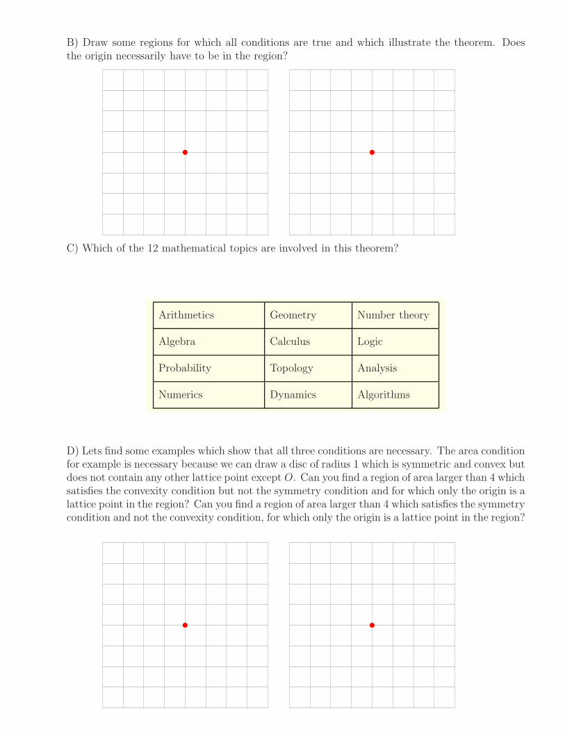
B) Draw some regions for which all conditions are true and which illustrate the theorem. Doesthe origin necessarily have to be in the region?

C) Which of the 12 mathematical topics are involved in this theorem?

Arithmetics Geometry Number theory

Algebra Calculus Logic

Probability Topology Analysis

Numerics Dynamics Algorithms

D) Lets find some examples which show that all three conditions are necessary. The area conditionfor example is necessary because we can draw a disc of radius 1 which is symmetric and convex butdoes not contain any other lattice point except O. Can you find a region of area larger than 4 whichsatisfies the convexity condition but not the symmetry condition and for which only the origin is alattice point in the region? Can you find a region of area larger than 4 which satisfies the symmetrycondition and not the convexity condition, for which only the origin is a lattice point in the region?

E-320: Teaching Math with a Historical Perspective

Oliver Knill, Harvard Extension, Spring 2014

Key information:

• URL: http://www.math.harvard.edu/knill/teaching/mathe320 2014

• Class: One Story Str. 307, 5:30-

7:30PM

• First Class: Mo, Jan 27, 2014

• Instructor: Oliver Knill, 432 Sci-

ence Center, knill@math.harvard.edu

• Office hours: Before and after the

lecture and by appointment.

• Text: Stillwell, Mathematics and its

History

Abstract:

The process of learning mathematics correlates with the history of math-

ematics. The struggle of research mathematicians developing a topic is

similar to the challenges we have to learn it. When learning the concept

of limits and series for example we undergo a similar process as the pio-

neers of a subject did when they developed the subject. This continues

to happen, as new flavors of calculus are developed and studied. We will

consider each week a different mathematical subject and pinpoint mo-

ments of of interest. We condense this into concrete working problems.

Prerequisites:

The presentation part should be generally accessible. While a pre-calculus

background is of advantage, an open mind is more important. Interest-

ing and new mathematics can be enjoyed also without vast background

knowledge.

Methodology:

We use the ”case method” methodology in which many different fields

mathematics can be covered. The range of mathematical topics is broad.

The main goal is to stimulate interest rather than cover a lot of ground.

After a general overview of Mathematics in the first lecture, we will work

each week with a specific branch of mathematics and see its development

in a historical context. The case method can be complemented with

a encyclopedic approach which has its value too. The advantage of

the case method is that one can pick concrete examples. As a balance,

we encourage to read in a book. A specific story is more engaging and

each ”case” can serve as a crystallization point for an entire subject.

In a time, when knowledge explodes fast and a plethora of possibilities

are offered online, teaching requires both to be broad as well as care

for details. The dilemma of combining these two can be achieved with

a ”short story approach” and also by mixing different teaching elements

like presentation, discussion and work problems. The case method is well

established like at business schools, where ”discussions focused on real-

world situations” is considered a good way to prepare students. In our

case, the ”real word situations” are ”historical highlights”. Participants

can adapt such models for their own teaching. Besides the material,

pedagogical questions will play an important role. One main theme will

be a general general principle: difficulties for the pioneers developing a

topic, reverberate today in the classroom when students are taught the

subject.

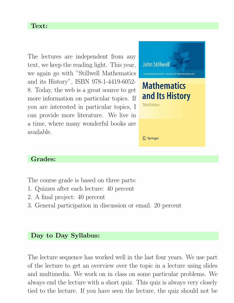
Text:

The lectures are independent from any

text, we keep the reading light. This year,

we again go with ”Stillwell Mathematics

and its History”, ISBN 978-1-4419-6052-

8. Today, the web is a great source to get

more information on particular topics. If

you are interested in particular topics, I

can provide more literature. We live in

a time, where many wonderful books are

available.

Grades:

The course grade is based on three parts:

1. Quizzes after each lecture: 40 percent

2. A final project: 40 percent

3. General participation in discussion or email. 20 percent

Day to Day Syllabus:

The lecture sequence has worked well in the last four years. We use part

of the lecture to get an overview over the topic in a lecture using slides

and multimedia. We work on in class on some particular problems. We

always end the lecture with a short quiz. This quiz is always very closely

tied to the lecture. If you have seen the lecture, the quiz should not be

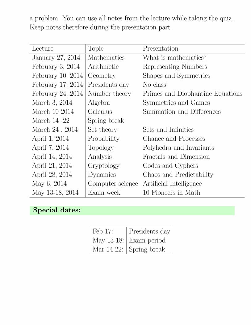
a problem. You can use all notes from the lecture while taking the quiz.

Keep notes therefore during the presentation part.

Lecture Topic Presentation

January 27, 2014 Mathematics What is mathematics?

February 3, 2014 Arithmetic Representing Numbers

February 10, 2014 Geometry Shapes and Symmetries

February 17, 2014 Presidents day No class

February 24, 2014 Number theory Primes and Diophantine Equations

March 3, 2014 Algebra Symmetries and Games

March 10 2014 Calculus Summation and Differences

March 14 -22 Spring break

March 24 , 2014 Set theory Sets and Infinities

April 1, 2014 Probability Chance and Processes

April 7, 2014 Topology Polyhedra and Invariants

April 14, 2014 Analysis Fractals and Dimension

April 21, 2014 Cryptology Codes and Cyphers

April 28, 2014 Dynamics Chaos and Predictability

May 6, 2014 Computer science Artificial Intelligence

May 13-18, 2014 Exam week 10 Pioneers in Math

Special dates:

Feb 17: Presidents day

May 13-18: Exam period

Mar 14-22: Spring break