Lecture 13: Cox PHM Part II

Basic Cox ModelParameter EstimationHypothesis Testing

Recall Basic Cox PHM

• Model

• Linear form

• Proportional hazards because

Likelihood

• Full likelihood

• Log-likelihood

Partial Likelihood

• The partial likelihood is defined as

• Where– j = 1, 2, …, n– No ties– t1 < t2 < … < tD

– Z(i)k is the kth covariate associated with the individual whose failure time is ti

– R(ti) is the risk set at time ti

1

11

exp

expi

pD k ikk

pi

k jkj R t k

ZL

Z

Estimation

• We can use the log of the likelihood to obtain and MLE for b

• Maximize log-likelihood to solve for estimates of b

• Score equations and information matrices are found using standard approaches

• Solving for estimates can be done numerically (e.g. Newton-Raphson)

Tests of the Model

• Testing that bk = 0 for all k = 1, 2, …, p

• Three main tests– Chi-square/ Wald test– Likelihood ratio test– Score test

• All three have chi-square distribution with p degrees of freedom

Score Equations an Information Matrix

• MLE found by Uh(b) = 0 using Newton-Raphson (need Uh(b) and I(b)).

• Start with an initial guess for b• After ith step of the algorithm the updated guess is

• Repeat this process until convergence achieved

11i k k kU

I

Developing the Tests

• In order to develop the tests, we must be able to define– Log-likelihood for the partial likelihood expression– The score equation(s) Uh(b)

– The information matrix I(b)

• A simple example…– 3 observed times: ti = t1 < t2 < t3

– Event indicators: di = 1, 1, 0

– 1 covariate: zi = z1, z2, z3

Log-likelihood

Log-likelihood

Score Equation

Score Equation

Information (Matrix)

Information (Matrix)

Information (Matrix)

Wald Test

• Based on:

• Wald test:

11 1

ˆ ˆ~ ,p pMVN I

0 0 0

'2

0 0

2 20

: . :

ˆ ˆ ˆ

~ under

A

W

W p

H vs H

X

X H

I

Score Test

• Based on:

• Score test:

'

1 2, ,...,

~ ,

pU U U U

U MVN

0 I

0 0 0

'2 1

0 0 0

2 20

: . :

~ under

A

Score

Score p

H vs H

X U U

X H

I

Likelihood Ratio Test

0 0 0

20

2 20

: . :

2 log log

~ under

A

LR

LR p

H vs H

X L L

X H

Partial Likelihood for Ties?

• The previous partial likelihood only applies when there are no ties

• Three primary approaches– Breslow– Efron– Cox

• When ties are few, all three perform similarly

Breslow (1974)

• si is the sum of the vectors Zj over all individuals who die at time ti

• Consider each of the di events at a given time as distinct

1

exp

expi

i

tDi

dti

jj R t

sL

Z

Efron (1977)

• Di is the set of individuals who have the event at time ti

• Closer to the correct partial likelihood score based on a discrete hazard model than Breslow’s

1

11

exp

exp expi

ii i

tDi

d jt ti

k kdk R t kj

sL

Z Z

Cox (1972)

• Based on discrete time, hazard-rate model• Assumes logistic model for hazard rate– Let h(t | Z) be the conditional death probability in

(t, t + 1) given survival to time t– Assume

0

0

exp11

th t Z h t

Zh th t Z

• This is the “proper” partial likelihood

• Where– Qi = a di – tuple of individuals who could have

been one of the di failures at ti

– q = {q1, q2, …, qdi } is one of the elements of Qi

– .

Cox (1972)- Discrete

*

1

exp

expi

tDi

ti qq Q

sL

s

*

1

jd

q qjjs z

Why Not Use Cox Every Time?

• Consider the computation• Denominator of Cox partial likelihood is more

complicated• Efron and Breslow approaches are less

intensive to calculate• R can do all three

“Local” Tests

• Testing individual coefficients• But, more interestingly, testing a set of coefficients• Examples– Testing treatment variables (3 categories)– Testing extent spread (4 categories)

• Same as previous– Wald test– Score test– Likelihood ratio test

Wald test• Partition • H0: • Based on maximum partial likelihood

estimators of • Let b = (b1, b2) be the maximum partial

likelihood estimator of b.• Partition the information matrix

1 2,

1 10

11 12

21 22

I II

I I

Wald test

• The Wald test is then

• Where I11(b) is the upper qxq submatrix of I(b)

• This statistics is distributed ~c2 with q degrees of freedom

' 121 10 11 1 1 10WX

b I b b

Score Test

• Define

• This is the vector of q scores for , evaluated at• The score test is then

• This statistics is distributed ~c2 with q degrees of freedom

1 10 2 10, U b

1

10

'2

1 10 2 10 11 10 2 10 1 10 2 10, , ,ScoreX U b I b U b

Likelihood Ratio Test

• Define b2(b10) be the partial maximum likelihood estimates of b2 based on the model with b1 set to b10

• The LRT is

• Where LL = log-likelihood• LRT has ~ chi-square distribution with p degrees of

freedom under H0

210 2 102 ,LRX LL LL b b

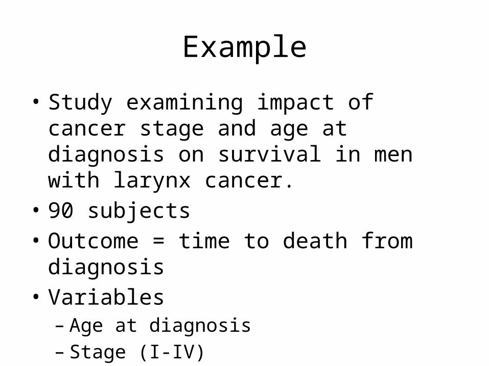
Example

• Study examining impact of cancer stage and age at diagnosis on survival in men with larynx cancer.

• 90 subjects• Outcome = time to death from diagnosis• Variables– Age at diagnosis– Stage (I-IV)

Model• Consider a model with both age and stage

• Global Tests (fit using Breslow method)– LRT: 18.07, p = 0.0012– Wald: 20.82, p = 0.0003 – Score: 24.33, p < 0.0001

Variable df beta se Wald Test p-value RR

Stage II 1 0.1386 0.4623 0.09 0.7644 1.15

Stage III 1 0.6383 0.3561 3.21 0.0730 1.89

Stage IV 1 1.6931 0.4222 16.08 <0.0001 5.44

Age 1 0.0189 0.0143 1.76 0.1874 1.02

Local Test

• Say we want to test whether or not the beta’s for stage are all 0…

• H0: • Necessary info depends on the test we want

to use– LRT: need log(L(b)) for “full” and “null” models– Wald: need b1 and I11

– Score: need U1[b10,b2(b10)] and I11(b10,b2(b10))

Stage II Stage III Stage IVˆ ˆ ˆ 0 . : at least 1 not = 0Avs H

Local Test: LRT• Null Model:

• Full Model:

• log(L(b)) for full model: -188.18• log(L(b)) for null model: -195.91

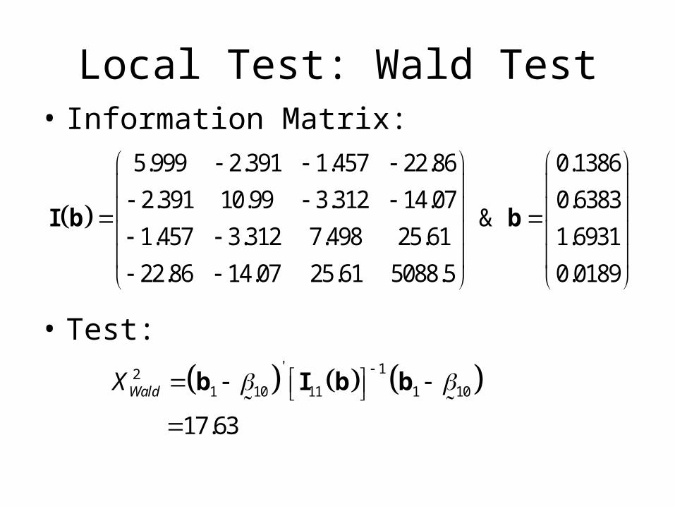
Local Test: Wald Test• Information Matrix:

• Test:

' 121 10 11 1 10

17.63

WaldX

b I b b

5.999 2.391 1.457 22.86 0.1386

2.391 10.99 3.312 14.07 0.6383&

1.457 3.312 7.498 25.61 1.6931

22.86 14.07 25.61 5088.5 0.0189

I b b

Local Test: Score Test• Vector of coefficients under null:

• Information matrix under null

• Test:

1'2 11

1 10 2 10 10 2 10 1 10 2 10, , ,

20.58

ScoreX

U b I b U b

0

7.637 2.608 0.699 24.73

2.608 9.994 0.979 8.429

0.699 0.979 3.174 11.31

24.73 8.429 11.31 4775.7

I

'

1 0 0 0 0.023 2.448 3.058 7.440 0.000 U

Contrasts

• Recall test for H0: c’b = c’b0

• When a covariate is a factor (e.g. stage), we can test contrasts – Stage II vs. Stage III– Stage II vs. Stage IV– Stage III vs. Stage IV

• Define scalar contrast matrix, c, and test H0: c’b = 0

Fitting Models In R

• coxph function for fitting CPHMs– Coefficient estimates– Global tests (LRT, Wald, and Score)– Local test for each individual covariate

• We can also easily conduct local tests ant contrasts using– LRT– Wald

• Score not so easy…

Example: Colon Cancer

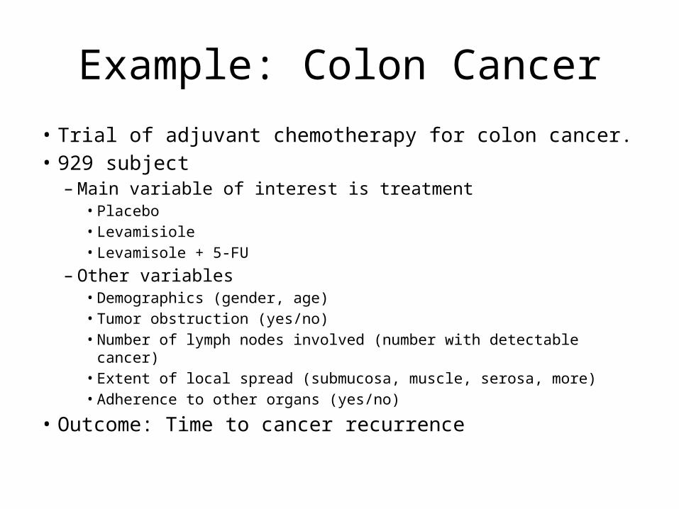
• Trial of adjuvant chemotherapy for colon cancer.• 929 subject

– Main variable of interest is treatment• Placebo• Levamisiole• Levamisole + 5-FU

– Other variables • Demographics (gender, age)• Tumor obstruction (yes/no)• Number of lymph nodes involved (number with detectable cancer)• Extent of local spread (submucosa, muscle, serosa, more)• Adherence to other organs (yes/no)

• Outcome: Time to cancer recurrence

Some of the Covariates

Fitting in R

• Treating factors as ordinalreg2<-coxph(st~sex+rx+perfor+obstruct+adhere+nodes2+ extent, data=coln)

• Treating factors as nominalreg3<-coxph(st~sex+rx+perfor+obstruct+adhere+factor(nodes2)+ factor(extent), data=coln)

Cox PHM Approach> data(colon)> coln<-colon[2*(1:929),]> st<-Surv(coln$time, coln$status)> reg1<-coxph(st~coln$rx)> attributes(reg1)$names [1] "coefficients" "var" "loglik" "score" "iter" "linear.predictors" [7] "residuals" "means" "concordance" "method" "n" "nevent" [13] "terms" "assign" "wald.test" "y" "formula" "xlevels" [19] "contrasts" "call"

$class[1] "coxph"

> reg1$coef coln$rxLev coln$rxLev+5FU -0.01512329 -0.51209312

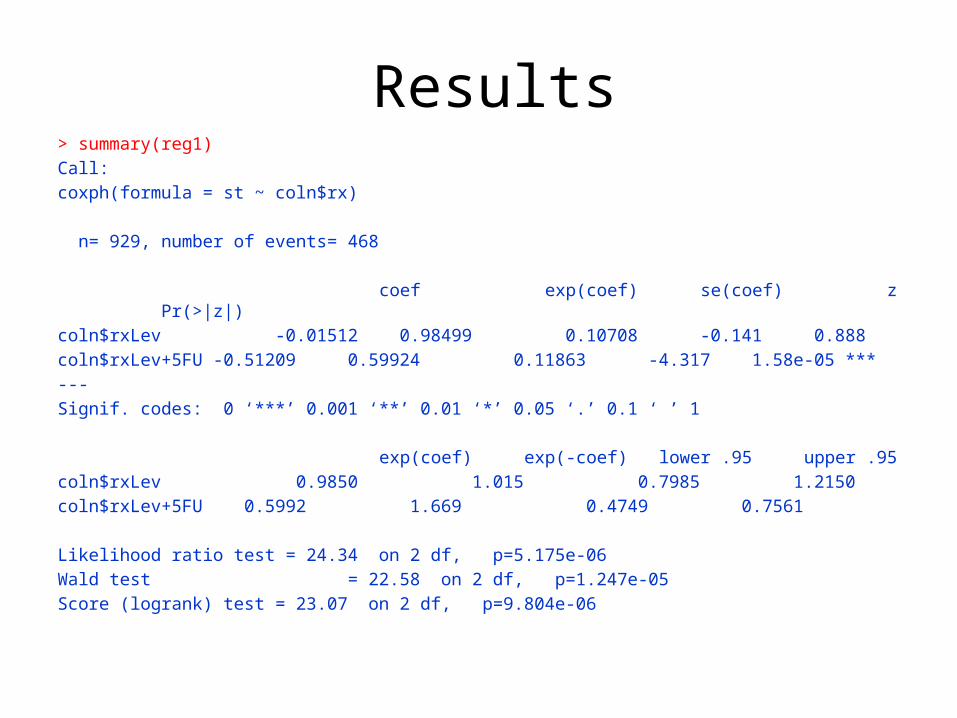
Results> summary(reg1)Call:coxph(formula = st ~ coln$rx)

n= 929, number of events= 468

coef exp(coef) se(coef) z Pr(>|z|) coln$rxLev -0.01512 0.98499 0.10708 -0.141 0.888 coln$rxLev+5FU -0.51209 0.59924 0.11863 -4.317 1.58e-05 ***---Signif. codes: 0 ‘***’ 0.001 ‘**’ 0.01 ‘*’ 0.05 ‘.’ 0.1 ‘ ’ 1

exp(coef) exp(-coef) lower .95 upper .95coln$rxLev 0.9850 1.015 0.7985 1.2150coln$rxLev+5FU 0.5992 1.669 0.4749 0.7561

Likelihood ratio test = 24.34 on 2 df, p=5.175e-06Wald test = 22.58 on 2 df, p=1.247e-05Score (logrank) test = 23.07 on 2 df, p=9.804e-06

Multiple Regression Results> summary(reg2)Call:coxph(formula = st ~ sex + rx + perfor + obstruct + adhere + nodes2 + extent, data = coln) n= 911, number of events= 456 (18 observations deleted due to missingness)

coef exp(coef) se(coef) z Pr(>|z|) sex -0.12256 0.88465 0.09410 -1.303 0.1927 rxLev -0.04272 0.95818 0.10833 -0.394 0.6933 rxLev+5FU -0.52460 0.59179 0.12077 -4.344 1.40e-05 ***perfor 0.07865 1.08182 0.25567 0.308 0.7584 obstruct 0.14509 1.15614 0.11649 1.245 0.2130 adhere 0.25080 1.28505 0.12656 1.982 0.0475 * nodes2 0.26254 1.30023 0.02995 8.765 < 2e-16 ***extent 0.53403 1.70579 0.11632 4.591 4.41e-06 ***--- Likelihood ratio test= 140.7 on 8 df, p=0Wald test = 134.3 on 8 df, p=0Score (logrank) test = 139.1 on 8 df, p=0

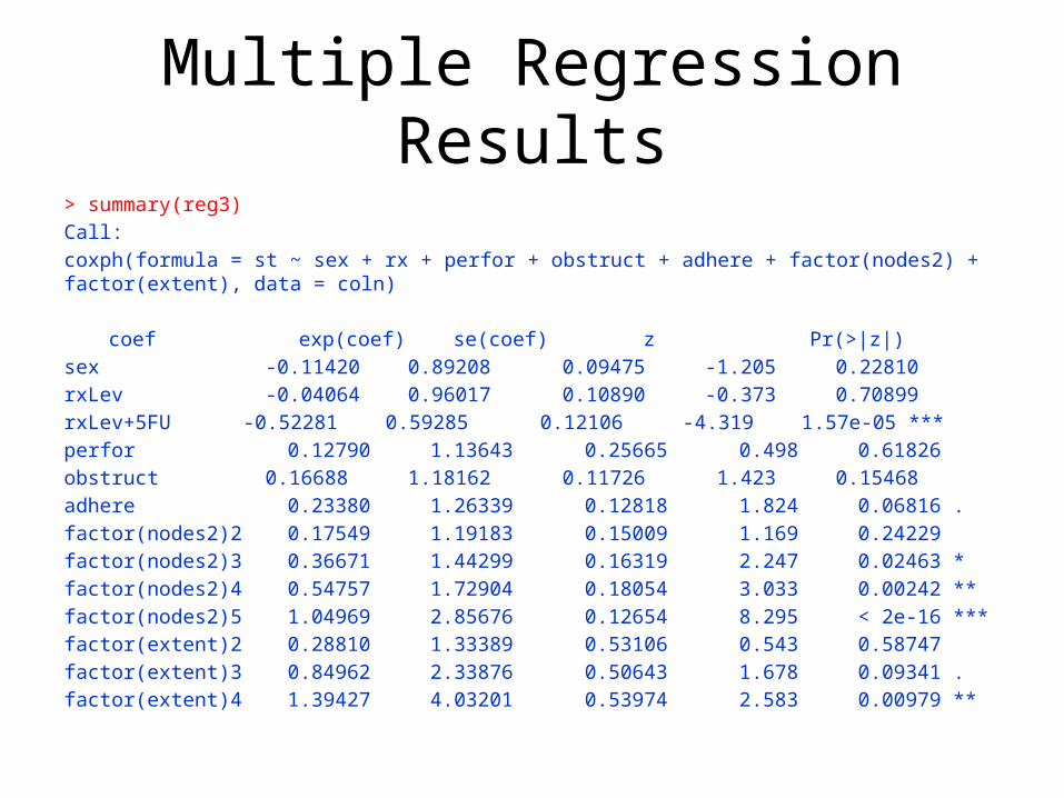
Multiple Regression Results> summary(reg3)Call:coxph(formula = st ~ sex + rx + perfor + obstruct + adhere + factor(nodes2) + factor(extent), data = coln)

coef exp(coef) se(coef) z Pr(>|z|) sex -0.11420 0.89208 0.09475 -1.205 0.22810 rxLev -0.04064 0.96017 0.10890 -0.373 0.70899 rxLev+5FU -0.52281 0.59285 0.12106 -4.319 1.57e-05 ***perfor 0.12790 1.13643 0.25665 0.498 0.61826 obstruct 0.16688 1.18162 0.11726 1.423 0.15468 adhere 0.23380 1.26339 0.12818 1.824 0.06816 . factor(nodes2)2 0.17549 1.19183 0.15009 1.169 0.24229 factor(nodes2)3 0.36671 1.44299 0.16319 2.247 0.02463 * factor(nodes2)4 0.54757 1.72904 0.18054 3.033 0.00242 ** factor(nodes2)5 1.04969 2.85676 0.12654 8.295 < 2e-16 ***factor(extent)2 0.28810 1.33389 0.53106 0.543 0.58747 factor(extent)3 0.84962 2.33876 0.50643 1.678 0.09341 . factor(extent)4 1.39427 4.03201 0.53974 2.583 0.00979 **

Ties?> table(duplicated(st))FALSE TRUE 751 1107 > coxph(st~rx, data=coln)

coef exp(coef) se(coef) z prxLev -0.0151 0.985 0.107 -0.141 8.9e-01rxLev+5FU -0.5121 0.599 0.119 -4.317 1.6e-05

Likelihood ratio test=24.3 on 2 df, p=5.17e-06 n= 929, number of events= 468

> coxph(st~rx, data=coln, ties="breslow")coef exp(coef) se(coef) z p

rxLev -0.0152 0.985 0.107 -0.142 8.9e-01rxLev+5FU -0.5119 0.599 0.119 -4.315 1.6e-05

Likelihood ratio test=24.3 on 2 df, p=5.23e-06 n= 929, number of events= 468

> coxph(st~rx, data=coln, ties="exact")coef exp(coef) se(coef) z p

rxLev -0.0152 0.985 0.107 -0.142 8.9e-01rxLev+5FU -0.5122 0.599 0.119 -4.317 1.6e-05

Likelihood ratio test=24.3 on 2 df, p=5.19e-06 n= 929, number of events= 468

Run Time

> system.time(coxph(st~rx, data=coln)) user system elapsed 0 0 0 > system.time(coxph(st~rx, data=coln, ties="breslow")) user system elapsed 0 0 0 > system.time(coxph(st~rx, data=coln, ties="exact")) user system elapsed 0.01 0.00 0.02

Local Tests

• Say we wanted to determine if extent of local spread mattered in the model

• Four categories:– 1 = submucosa – 2 = muscle– 3 = serosa– 4 = contiguous structures

• We can use our local tests here (must set it up ourselves in R)– LRT– Wald

Local Test: LRT> full_fit<-coxph(st ~ sex + rx + perfor + obstruct + adhere + factor(nodes2)+ factor(extent), data=coln)> LLfull<-full_fit$loglik[2]> LLfull[1] -2883.81

> null_fit<-coxph(st ~ sex + rx + perfor + obstruct + adhere + factor(nodes2), data=coln)> LLnull<-null_fit$loglik[2]> LLnull[1] -2895.227

> LRT_extent<-2*(LLfull-LLnull)> LRT_extent[1] 22.83403

> pval<-pchisq(LRT_extent, df=3, lower=F)> pval[1] 4.373093e-05

Local Test: Wald Test> reg3<-coxph(st~sex+rx+perfor+obstruct+adhere+factor(nodes2)+ factor(extent), data=coln)> wald_extent<-t(reg3$coeffic[11:13])%*%solve(reg3$var[11:13,11:13])%*% reg3$coeffic[11:13]> wald_extent [,1][1,] 21.25669

> pval<-pchisq(wald_extent, df=3, lower=F)> pval [,1][1,] 9.311276e-05

Contrasts

• Since at least one of the extent of spread categories was not 0, we may also want to contrast the four categories

• We can use contrasts but again, we must set this up ourselves in R.

Contrasts in R> E2vE3<-reg3$coef[11:12]%*%c(-1,1)> se2v3<-sqrt(reg3$var[11,11]+reg3$var[12,12]-2*reg3$var[11,12])> z2v3<-E2vE3/se2v3> z2v3 [,1][1,] 2.730731> 2*(1-pnorm(abs(z2v3))) [,1][1,] 0.001843819 > E2vE4<-reg3$coef[c(11,13)]%*%c(-1,1)> se2v4<-sqrt(reg3$var[11,11]+reg3$var[13,13]-2*reg3$var[11,13])> z2v4<-E2vE4/se2v4> z2v4 [,1][1,] 4.286233> 2*(1-pnorm(abs(z2v4))) [,1][1,] 1.817281e-05

Confidence Interval

• Construct a 95% CI for the hazard ratio between different extent of local spread categories

• For specific model coefficient

• For a contrast

2

2

1

1

ˆ ˆbeta :

ˆ ˆHR : exp

k k

k k

z se

z se

2

2

1

1

ˆ ˆ ˆ ˆ ˆ ˆcontrast : var var 2cov ,

ˆ ˆ ˆ ˆ ˆ ˆHR : exp var var 2cov ,

k j k j k j

k j k j k j

z

z

CIs for Contrasts in R> ucv23<-E2vE3+qnorm(.975)*se2v3> lcv23<-E2vE3-qnorm(.975)*se2v3> hr23<-exp(E2vE3)> hr23 [,1][1,] 1.753335

> uhr23<-exp(ucv23)> uhr23 [,1][1,] 2.496546

> lhr23<-exp(lcv23)> lhr23 [,1][1,] 1.231374

Confidence Interval

• Conclusion: – Adjusting for other covariates in the model, the

risk of death among individuals with serosa involvement is 1.75 times the risk of death relative to subjects with only muscle involvement (95% CI for RR 1.23-2.50).

Proportional?

• Recall we are making a strong assumption that we have proportional hazards for each covariate

• We can investigate this to some extent via graphical displays

• BUT limited for quantitative variables• We’ll learn more about this later