Lecture 13 Linear dynamical systems with inputs & outputs · Inputs & outputs recall continuous-time time-invariant LDS has form x˙ = Ax+Bu, y = Cx+Du • Ax is called the drift

EE263 Autumn 2007-08 Stephen Boyd

Lecture 13Linear dynamical systems with inputs &

outputs

• inputs & outputs: interpretations

• transfer matrix

• impulse and step matrices

• examples

13–1

Inputs & outputs

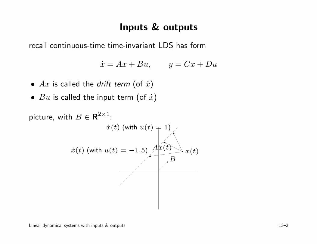
recall continuous-time time-invariant LDS has form

x = Ax + Bu, y = Cx + Du

• Ax is called the drift term (of x)

• Bu is called the input term (of x)

picture, with B ∈ R2×1:

x(t)Ax(t)

x(t) (with u(t) = 1)

x(t) (with u(t) = −1.5)

B

Linear dynamical systems with inputs & outputs 13–2

Interpretations

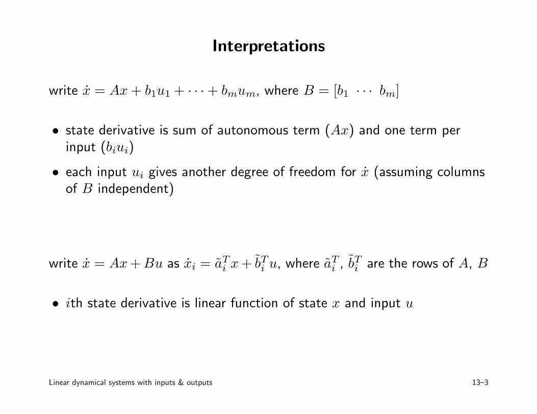
write x = Ax + b1u1 + · · · + bmum, where B = [b1 · · · bm]

• state derivative is sum of autonomous term (Ax) and one term perinput (biui)

• each input ui gives another degree of freedom for x (assuming columnsof B independent)

write x = Ax + Bu as xi = aTi x + bT

i u, where aTi , bT

i are the rows of A, B

• ith state derivative is linear function of state x and input u


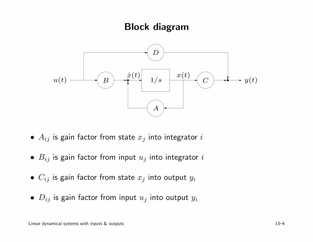
Block diagram

1/s

A

B C

D

x(t)x(t)u(t) y(t)

• Aij is gain factor from state xj into integrator i

• Bij is gain factor from input uj into integrator i

• Cij is gain factor from state xj into output yi

• Dij is gain factor from input uj into output yi


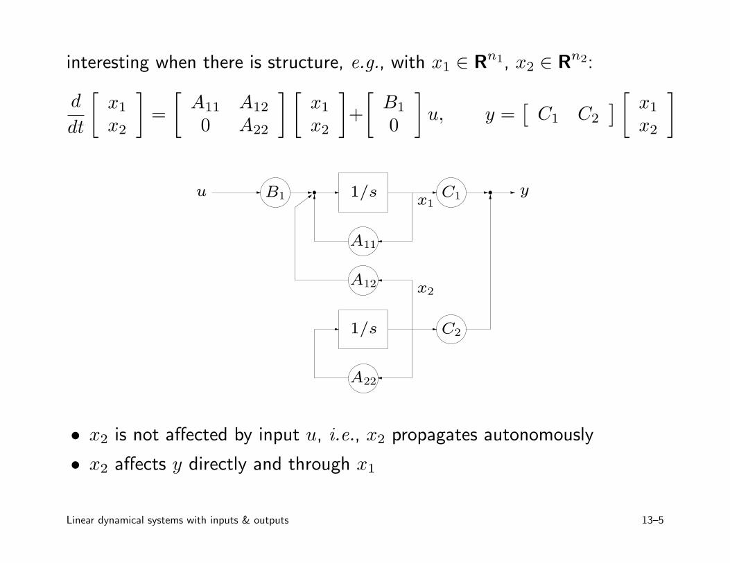
interesting when there is structure, e.g., with x1 ∈ Rn1, x2 ∈ Rn2:

d

dt

[

x1

x2

]

=

[

A11 A12

0 A22

] [

x1

x2

]

+

[

B1

0

]

u, y =[

C1 C2

]

[

x1

x2

]

1/s

1/s

A11

A12

A22

B1 C1

C2

x1

x2

u y

• x2 is not affected by input u, i.e., x2 propagates autonomously

• x2 affects y directly and through x1


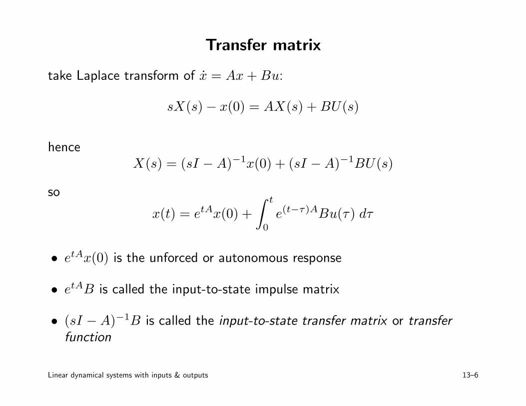
Transfer matrix

take Laplace transform of x = Ax + Bu:

sX(s) − x(0) = AX(s) + BU(s)

henceX(s) = (sI − A)−1x(0) + (sI − A)−1BU(s)

so

x(t) = etAx(0) +

∫ t

0

e(t−τ)ABu(τ) dτ

• etAx(0) is the unforced or autonomous response

• etAB is called the input-to-state impulse matrix

• (sI − A)−1B is called the input-to-state transfer matrix or transfer

function


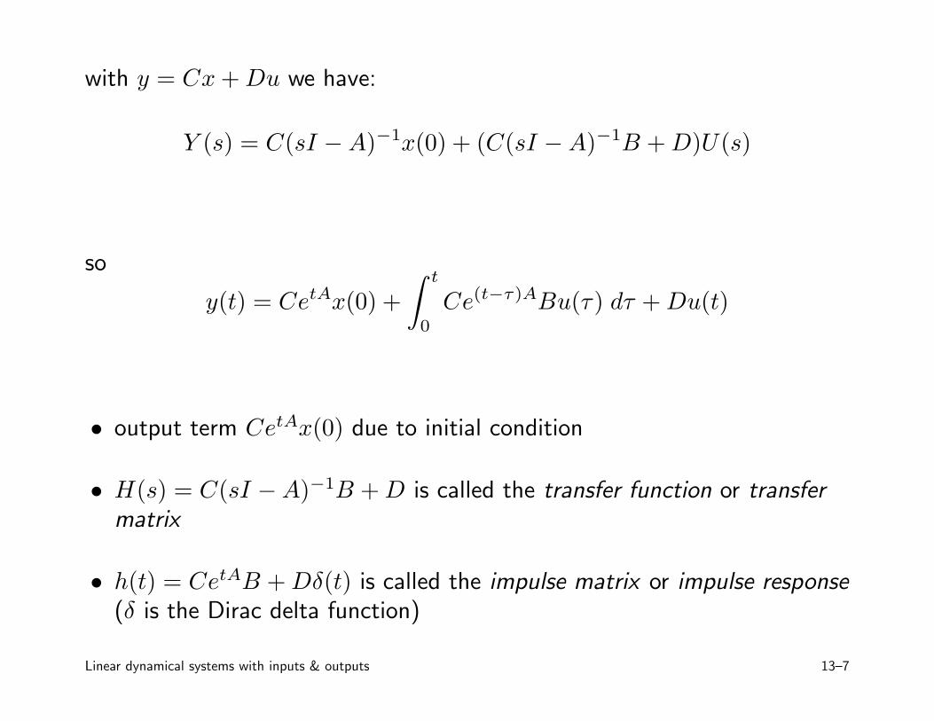
with y = Cx + Du we have:

Y (s) = C(sI − A)−1x(0) + (C(sI − A)−1B + D)U(s)

so

y(t) = CetAx(0) +

∫ t

0

Ce(t−τ)ABu(τ) dτ + Du(t)

• output term CetAx(0) due to initial condition

• H(s) = C(sI − A)−1B + D is called the transfer function or transfer

matrix

• h(t) = CetAB + Dδ(t) is called the impulse matrix or impulse response

(δ is the Dirac delta function)


with zero initial condition we have:

Y (s) = H(s)U(s), y = h ∗ u

where ∗ is convolution (of matrix valued functions)

intepretation:

• Hij is transfer function from input uj to output yi


Impulse matrix

impulse matrix h(t) = CetAB + Dδ(t)

with x(0) = 0, y = h ∗ u, i.e.,

yi(t) =

m∑

j=1

∫ t

0

hij(t − τ)uj(τ) dτ

interpretations:

• hij(t) is impulse response from jth input to ith output

• hij(t) gives yi when u(t) = ejδ

• hij(τ) shows how dependent output i is, on what input j was, τseconds ago

• i indexes output; j indexes input; τ indexes time lag


Step matrix

the step matrix or step response matrix is given by

s(t) =

∫ t

0

h(τ) dτ

interpretations:

• sij(t) is step response from jth input to ith output

• sij(t) gives yi when u = ej for t ≥ 0

for invertible A, we have

s(t) = CA−1(

etA − I)

B + D


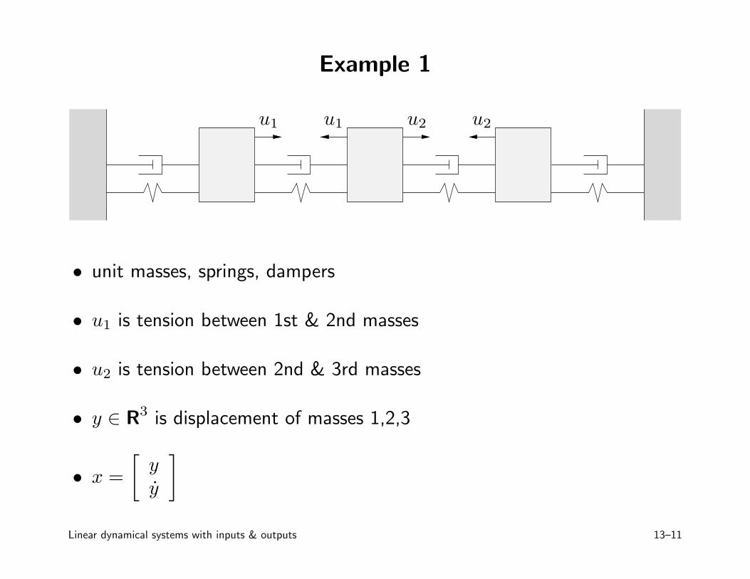
Example 1

u1 u2u1 u2

• unit masses, springs, dampers

• u1 is tension between 1st & 2nd masses

• u2 is tension between 2nd & 3rd masses

• y ∈ R3 is displacement of masses 1,2,3

• x =

[

yy

]


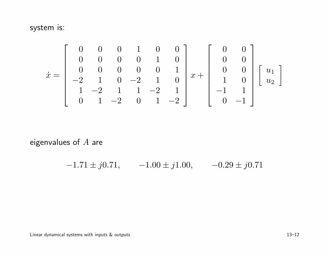
system is:

x =

0 0 0 1 0 00 0 0 0 1 00 0 0 0 0 1

−2 1 0 −2 1 01 −2 1 1 −2 10 1 −2 0 1 −2

x +

0 00 00 01 0

−1 10 −1

[

u1

u2

]

eigenvalues of A are

−1.71 ± j0.71, −1.00 ± j1.00, −0.29 ± j0.71


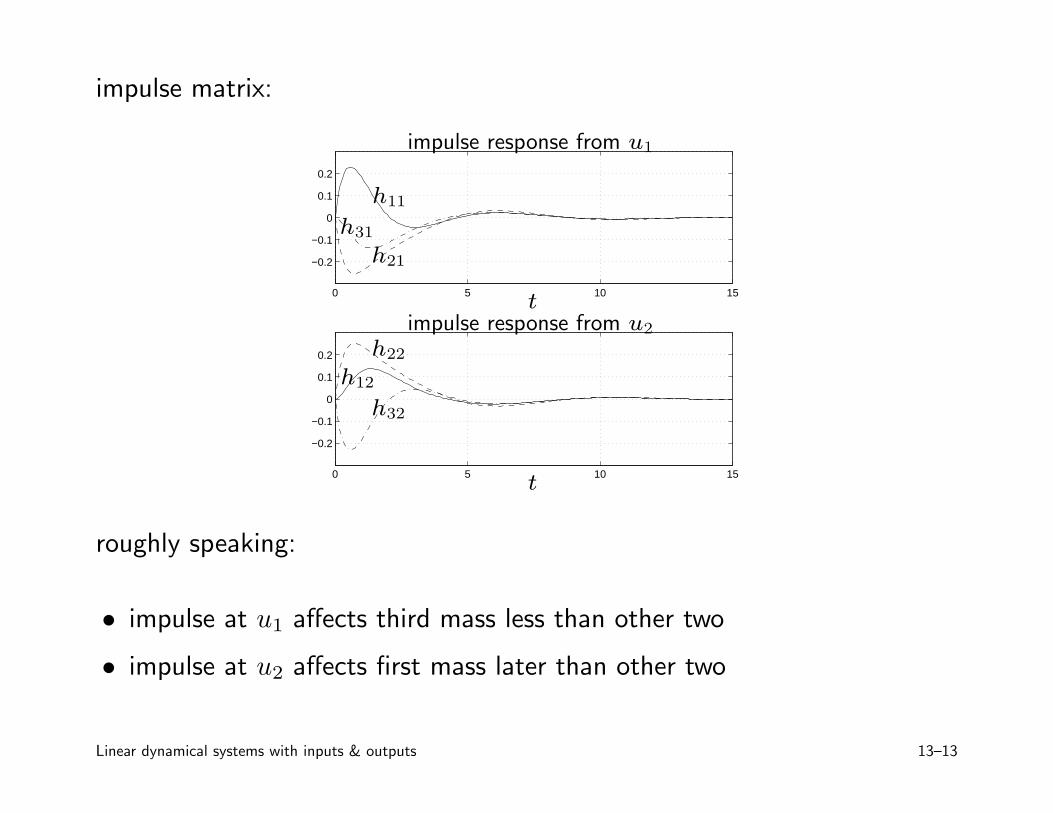
impulse matrix:

0 5 10 15

−0.2

−0.1

0

0.1

0.2

0 5 10 15

−0.2

−0.1

0

0.1

0.2

t

t

h11

h21

h31

h12

h22

h32

impulse response from u1

impulse response from u2

roughly speaking:

• impulse at u1 affects third mass less than other two

• impulse at u2 affects first mass later than other two


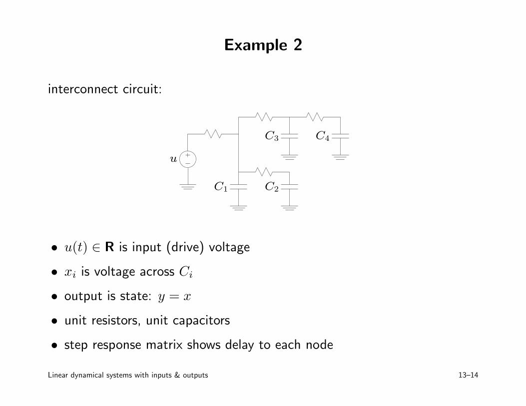
Example 2

interconnect circuit:

u

C3 C4

C1 C2

• u(t) ∈ R is input (drive) voltage

• xi is voltage across Ci

• output is state: y = x

• unit resistors, unit capacitors

• step response matrix shows delay to each node


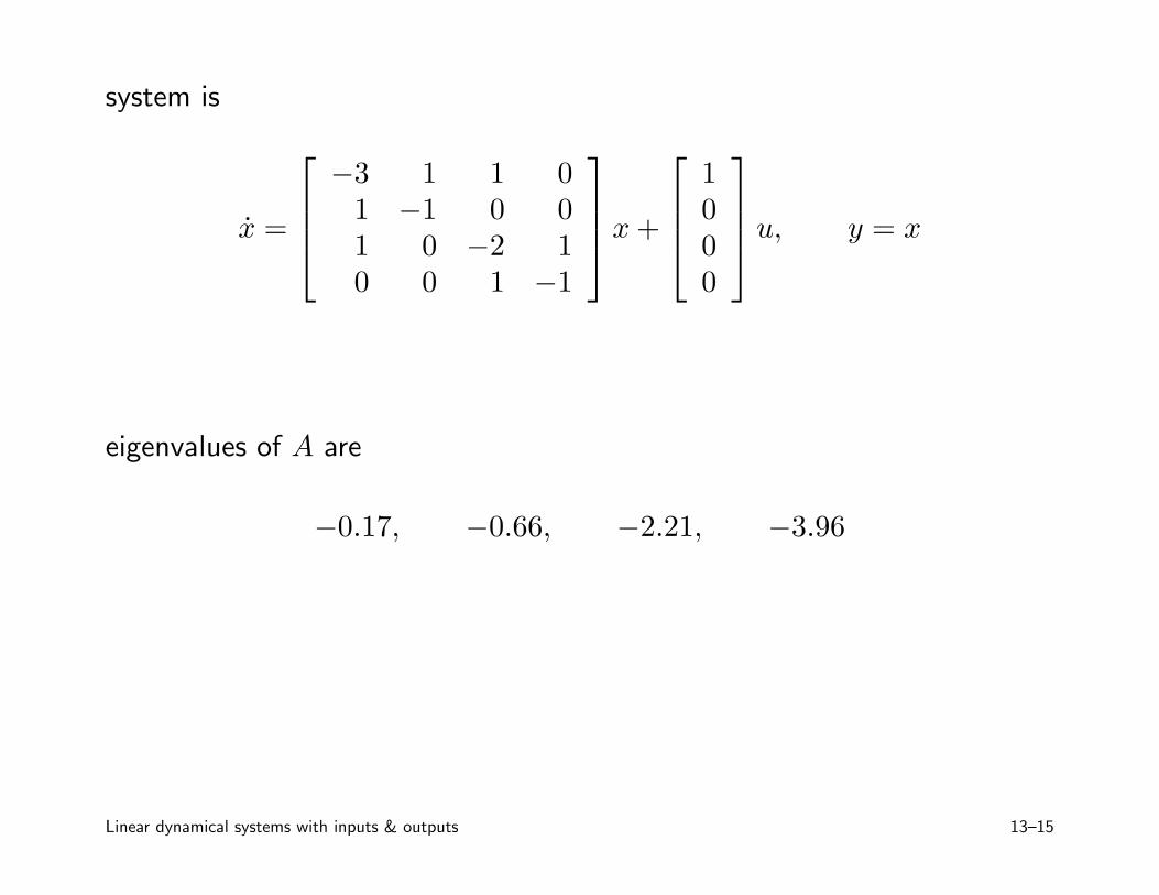
system is

x =

−3 1 1 01 −1 0 01 0 −2 10 0 1 −1

x +

1000

u, y = x

eigenvalues of A are

−0.17, −0.66, −2.21, −3.96


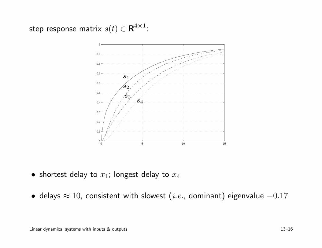
step response matrix s(t) ∈ R4×1:

0 5 10 150

0.1

0.2

0.3

0.4

0.5

0.6

0.7

0.8

0.9

1

s1

s2

s3s4

• shortest delay to x1; longest delay to x4

• delays ≈ 10, consistent with slowest (i.e., dominant) eigenvalue −0.17


DC or static gain matrix

• transfer matrix at s = 0 is H(0) = −CA−1B + D ∈ Rm×p

• DC transfer matrix describes system under static conditions, i.e., x, u,y constant:

0 = x = Ax + Bu, y = Cx + Du

eliminate x to get y = H(0)u

• if system is stable,

H(0) =

∫

∞

0

h(t) dt = limt→∞

s(t)

(recall: H(s) =

∫

∞

0

e−sth(t) dt, s(t) =

∫ t

0

h(τ) dτ)

if u(t) → u∞ ∈ Rm, then y(t) → y∞ ∈ Rp where y∞ = H(0)u∞


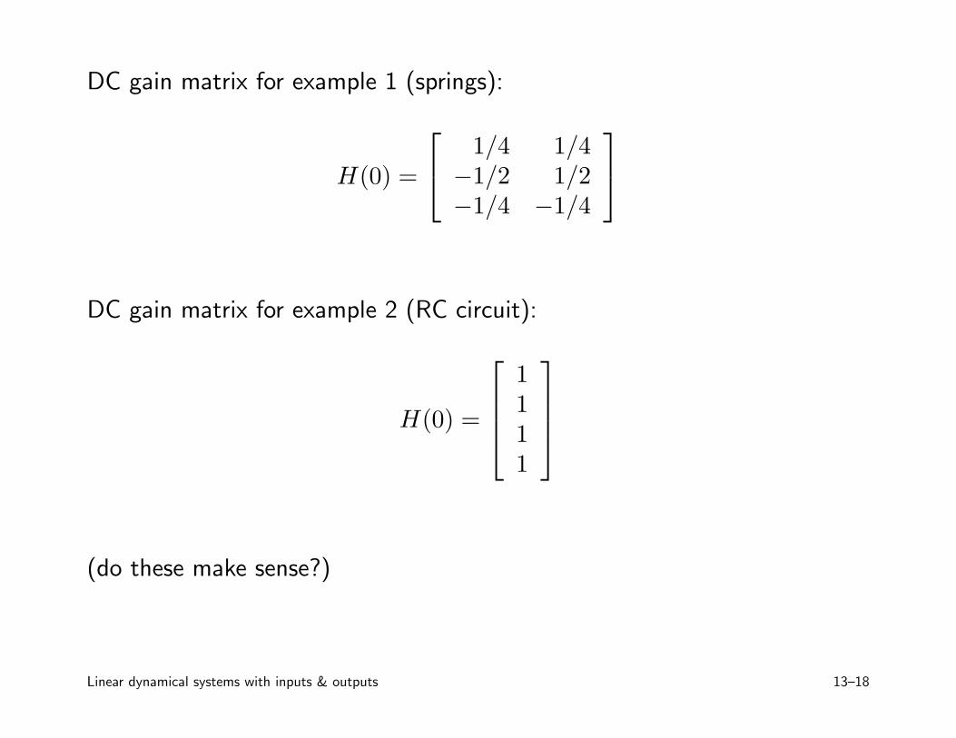
DC gain matrix for example 1 (springs):

H(0) =

1/4 1/4−1/2 1/2−1/4 −1/4

DC gain matrix for example 2 (RC circuit):

H(0) =

1111

(do these make sense?)


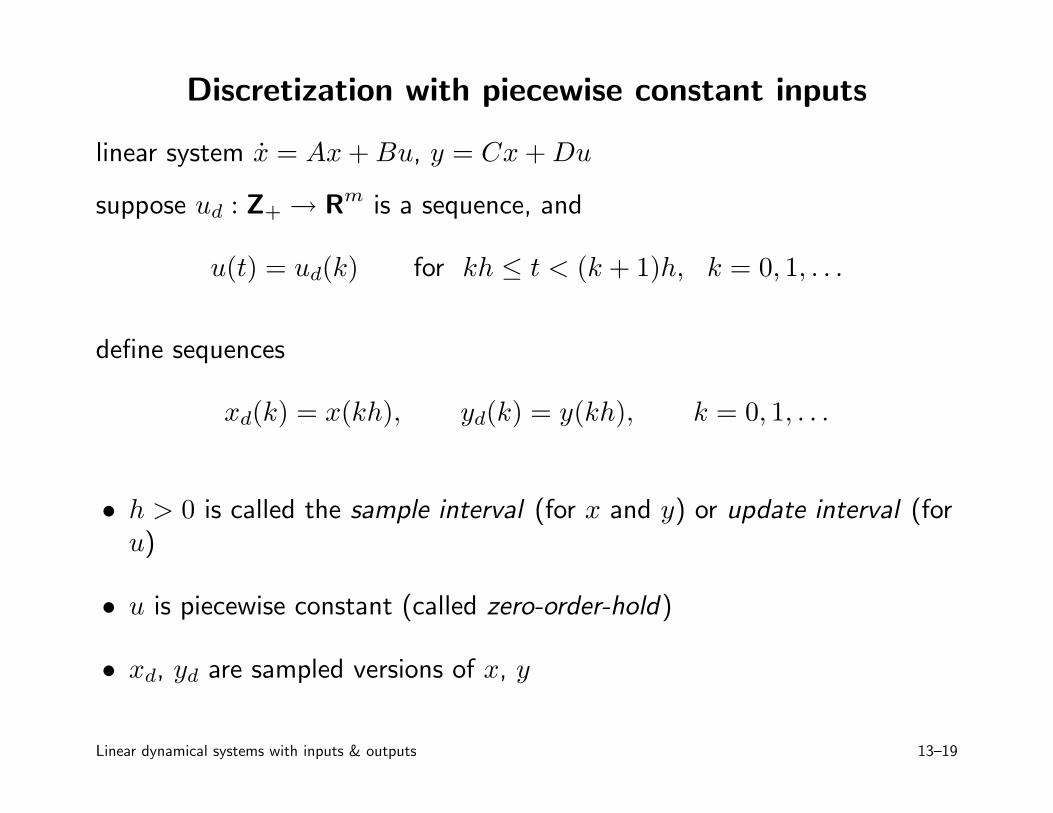
Discretization with piecewise constant inputs

linear system x = Ax + Bu, y = Cx + Du

suppose ud : Z+ → Rm is a sequence, and

u(t) = ud(k) for kh ≤ t < (k + 1)h, k = 0, 1, . . .

define sequences

xd(k) = x(kh), yd(k) = y(kh), k = 0, 1, . . .

• h > 0 is called the sample interval (for x and y) or update interval (foru)

• u is piecewise constant (called zero-order-hold)

• xd, yd are sampled versions of x, y


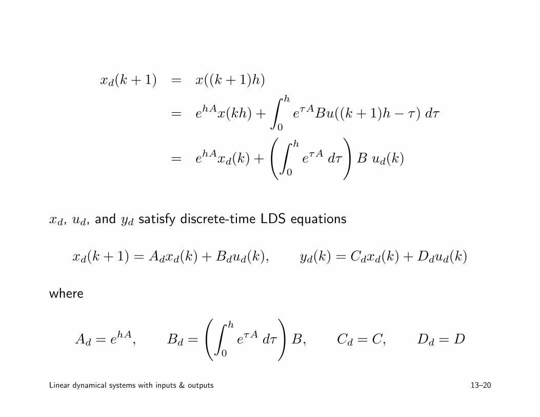
xd(k + 1) = x((k + 1)h)

= ehAx(kh) +

∫ h

0

eτABu((k + 1)h − τ) dτ

= ehAxd(k) +

(

∫ h

0

eτA dτ

)

B ud(k)

xd, ud, and yd satisfy discrete-time LDS equations

xd(k + 1) = Adxd(k) + Bdud(k), yd(k) = Cdxd(k) + Ddud(k)

where

Ad = ehA, Bd =

(

∫ h

0

eτA dτ

)

B, Cd = C, Dd = D


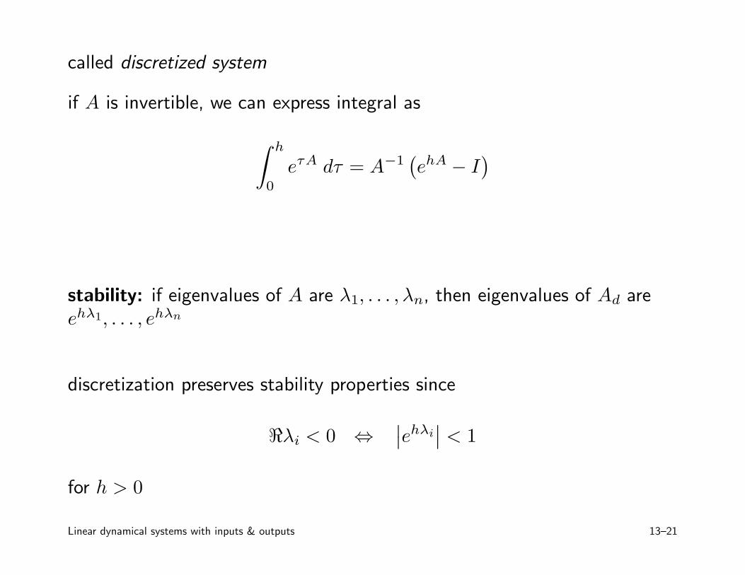
called discretized system

if A is invertible, we can express integral as

∫ h

0

eτA dτ = A−1(

ehA − I)

stability: if eigenvalues of A are λ1, . . . , λn, then eigenvalues of Ad areehλ1, . . . , ehλn

discretization preserves stability properties since

ℜλi < 0 ⇔∣

∣ehλi∣

∣ < 1

for h > 0


extensions/variations:

• offsets: updates for u and sampling of x, y are offset in time

• multirate: ui updated, yi sampled at different intervals

(usually integer multiples of a common interval h)

both very common in practice


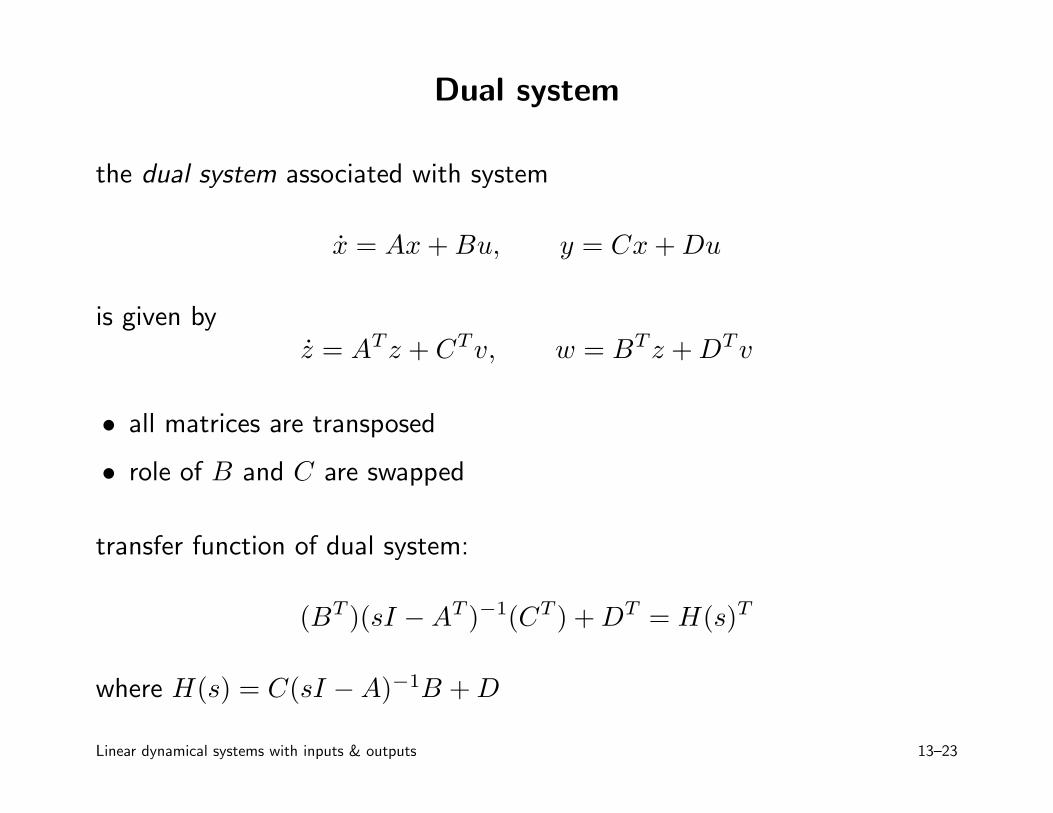
Dual system

the dual system associated with system

x = Ax + Bu, y = Cx + Du

is given byz = ATz + CTv, w = BTz + DTv

• all matrices are transposed

• role of B and C are swapped

transfer function of dual system:

(BT )(sI − AT )−1(CT ) + DT = H(s)T

where H(s) = C(sI − A)−1B + D


(for SISO case, TF of dual is same as original)

eigenvalues (hence stability properties) are the same


Dual via block diagram

in terms of block diagrams, dual is formed by:

• transpose all matrices

• swap inputs and outputs on all boxes

• reverse directions of signal flow arrows

• swap solder joints and summing junctions


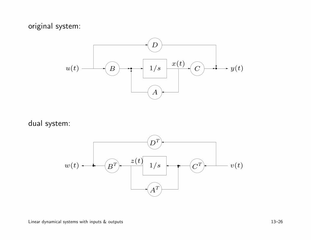
original system:

1/s

A

B C

D

x(t)u(t) y(t)

dual system:

1/s

AT

BT CT

DT

z(t)w(t) v(t)


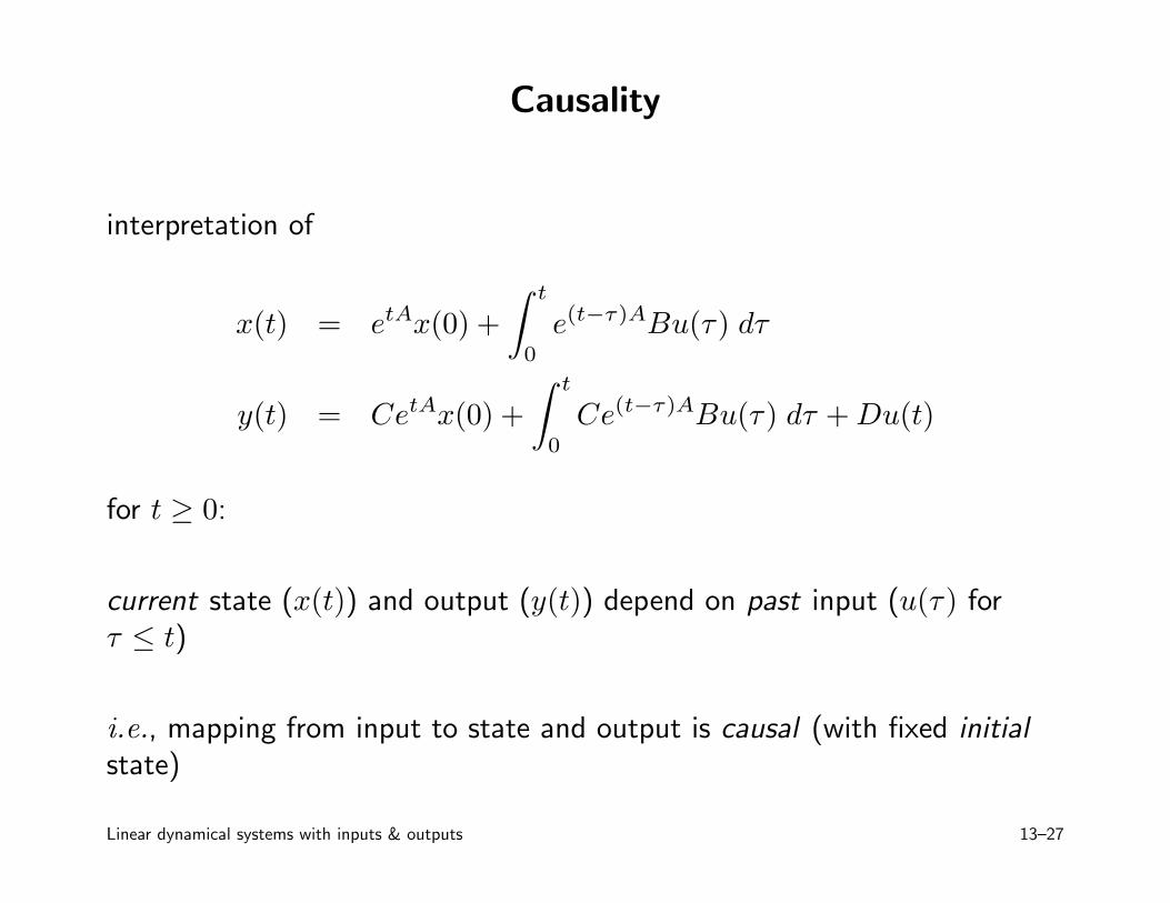
Causality

interpretation of

x(t) = etAx(0) +

∫ t

0

e(t−τ)ABu(τ) dτ

y(t) = CetAx(0) +

∫ t

0

Ce(t−τ)ABu(τ) dτ + Du(t)

for t ≥ 0:

current state (x(t)) and output (y(t)) depend on past input (u(τ) forτ ≤ t)

i.e., mapping from input to state and output is causal (with fixed initial

state)


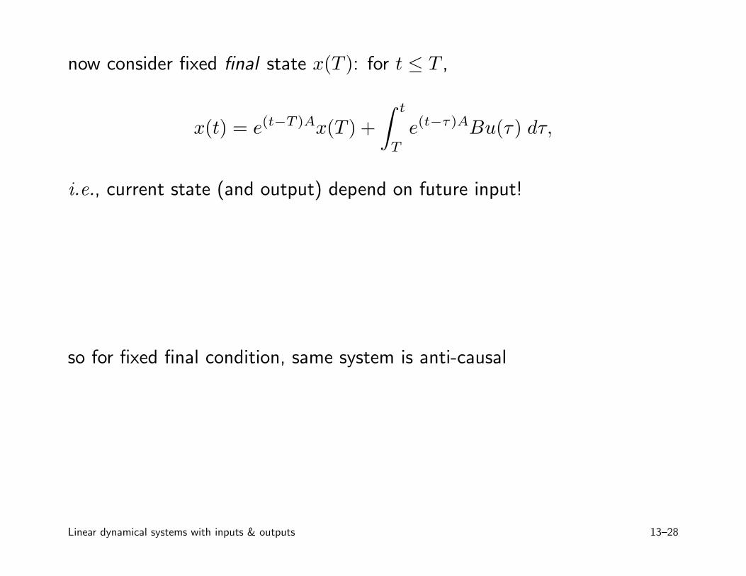
now consider fixed final state x(T ): for t ≤ T ,

x(t) = e(t−T )Ax(T ) +

∫ t

T

e(t−τ)ABu(τ) dτ,

i.e., current state (and output) depend on future input!

so for fixed final condition, same system is anti-causal


Idea of state

x(t) is called state of system at time t since:

• future output depends only on current state and future input

• future output depends on past input only through current state

• state summarizes effect of past inputs on future output

• state is bridge between past inputs and future outputs


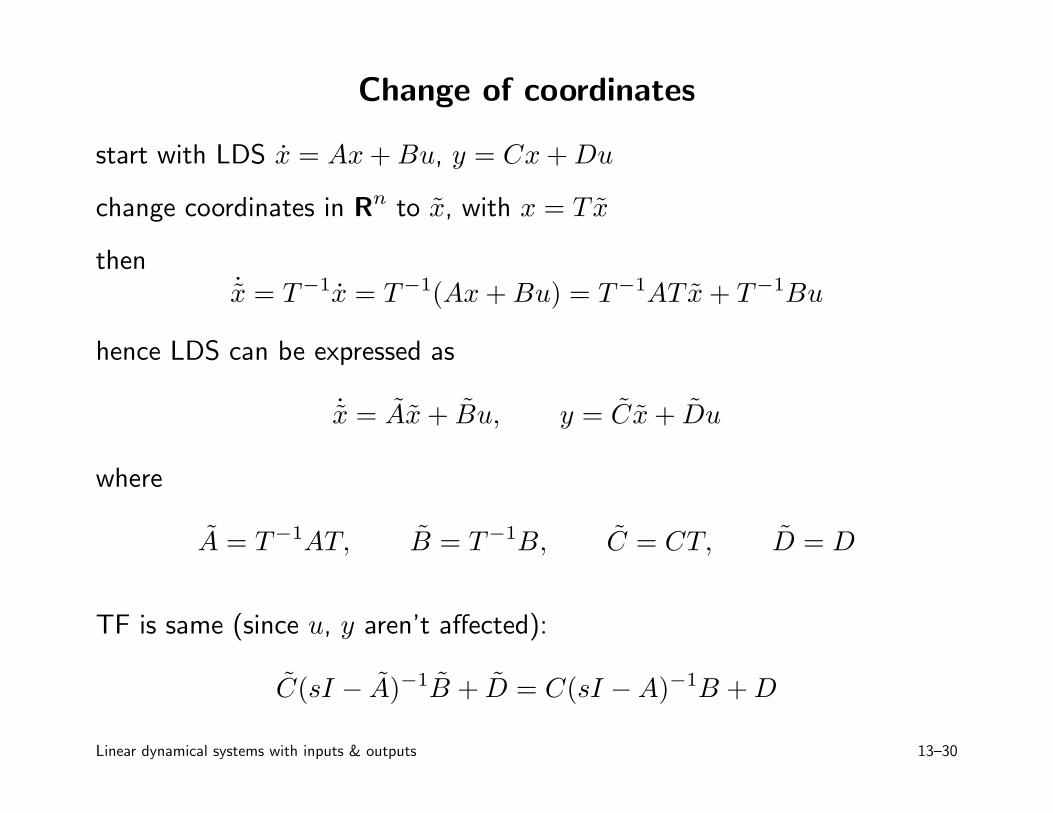
Change of coordinates

start with LDS x = Ax + Bu, y = Cx + Du

change coordinates in Rn to x, with x = T x

then˙x = T−1x = T−1(Ax + Bu) = T−1ATx + T−1Bu

hence LDS can be expressed as

˙x = Ax + Bu, y = Cx + Du

where

A = T−1AT, B = T−1B, C = CT, D = D

TF is same (since u, y aren’t affected):

C(sI − A)−1B + D = C(sI − A)−1B + D


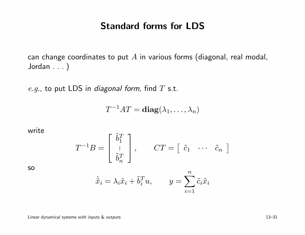
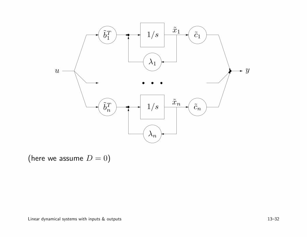
Standard forms for LDS

can change coordinates to put A in various forms (diagonal, real modal,Jordan . . . )

e.g., to put LDS in diagonal form, find T s.t.

T−1AT = diag(λ1, . . . , λn)

write

T−1B =

bT1...

bTn

, CT =[

c1 · · · cn

]

so

˙xi = λixi + bTi u, y =

n∑

i=1

cixi


1/s

1/sbT1

bTn

c1

cn

x1

xn

u yλ1

λn

(here we assume D = 0)


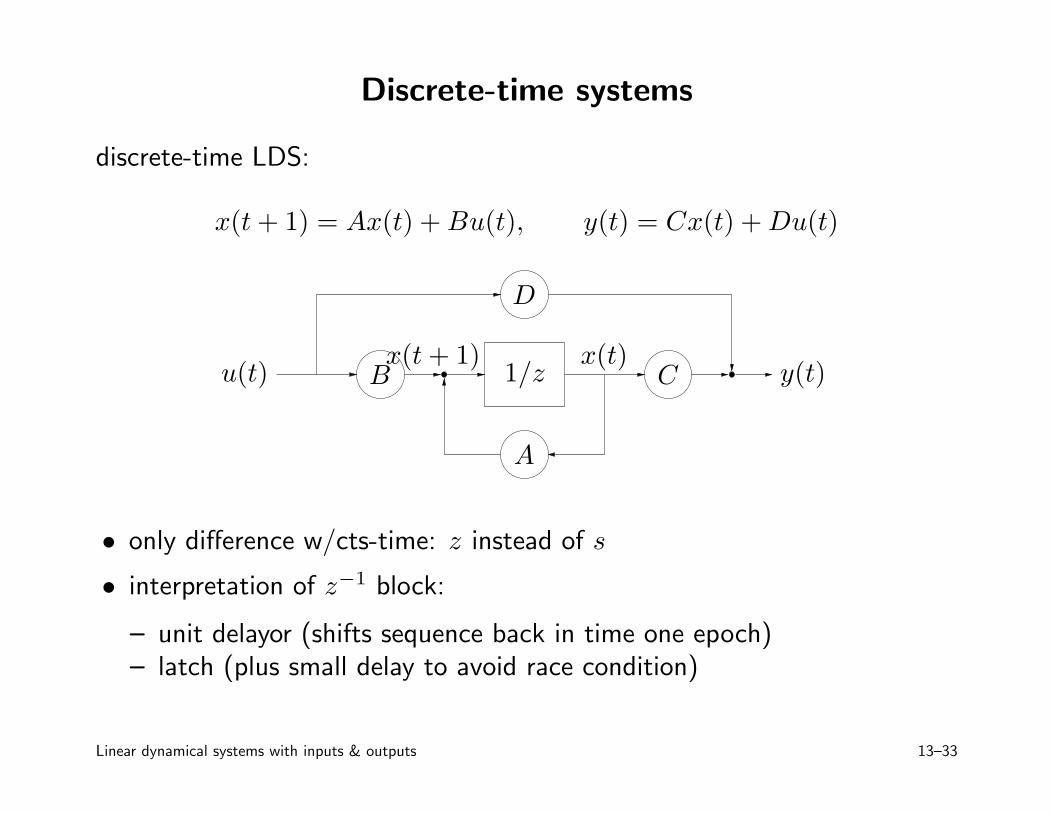
Discrete-time systems

discrete-time LDS:

x(t + 1) = Ax(t) + Bu(t), y(t) = Cx(t) + Du(t)

1/z

A

B C

D

x(t)x(t + 1)u(t) y(t)

• only difference w/cts-time: z instead of s

• interpretation of z−1 block:

– unit delayor (shifts sequence back in time one epoch)– latch (plus small delay to avoid race condition)


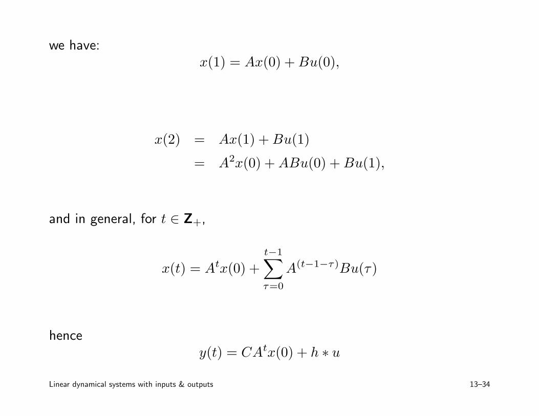
we have:x(1) = Ax(0) + Bu(0),

x(2) = Ax(1) + Bu(1)

= A2x(0) + ABu(0) + Bu(1),

and in general, for t ∈ Z+,

x(t) = Atx(0) +

t−1∑

τ=0

A(t−1−τ)Bu(τ)

hencey(t) = CAtx(0) + h ∗ u


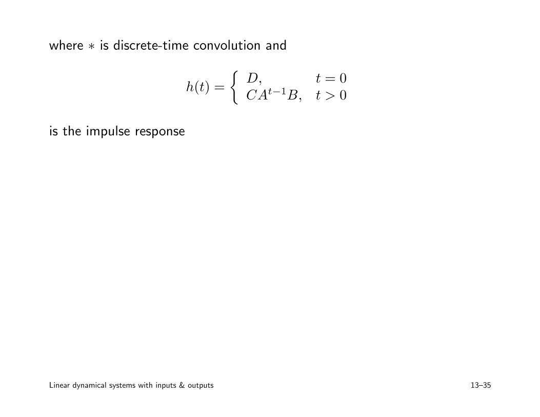
where ∗ is discrete-time convolution and

h(t) =

{

D, t = 0CAt−1B, t > 0

is the impulse response


Z-transform

suppose w ∈ Rp×q is a sequence (discrete-time signal), i.e.,

w : Z+ → Rp×q

recall Z-transform W = Z(w):

W (z) =

∞∑

t=0

z−tw(t)

where W : D ⊆ C → Cp×q (D is domain of W )

time-advanced or shifted signal v:

v(t) = w(t + 1), t = 0, 1, . . .


Z-transform of time-advanced signal:

V (z) =

∞∑

t=0

z−tw(t + 1)

= z

∞∑

t=1

z−tw(t)

= zW (z) − zw(0)


Discrete-time transfer function

take Z-transform of system equations

x(t + 1) = Ax(t) + Bu(t), y(t) = Cx(t) + Du(t)

yields

zX(z) − zx(0) = AX(z) + BU(z), Y (z) = CX(z) + DU(z)

solve for X(z) to get

X(z) = (zI − A)−1zx(0) + (zI − A)−1BU(z)

(note extra z in first term!)


henceY (z) = H(z)U(z) + C(zI − A)−1zx(0)

where H(z) = C(zI − A)−1B + D is the discrete-time transfer function

note power series expansion of resolvent:

(zI − A)−1 = z−1I + z−2A + z−3A2 + · · ·


Documents

Lecture 13 Linear dynamical systems with inputs & outputs · Inputs & outputs recall continuous-time time-invariant LDS has form x˙ = Ax+Bu, y = Cx+Du • Ax is called the drift