Lecture 16: Multiresolution Image Analysis

Harvey RhodyChester F. Carlson Center for Imaging Science

Rochester Institute of Technologyrhody@cis.rit.edu

November 9, 2004

AbstractMultiresolution analysis provides information on both the spatial

and frequency domains. Here we describe multiresolution analysisfrom a wavelet perspective and provide a simple example.

DIP Lecture 16

Multiresolution Analysis

The wavelet transform is the foundation of techniques for analysis,compression and transmission of images.

Mallat (1987) showed that wavelets unify a number of techniques,including subband coding (signal processing), quadrature mirror filtering(speech processing) and pyramidal coding (image processing). The namemultiresolution analysis has been used for these techniques.

DIP Lecture 16 1

Image Pyramid

Let A be an image of size N ×N where N = 2J .

Let AJ−1 be formed by smoothing A and then downsampling.

Let A be an approximation of A reconstructed by upsampling andinterpolating.

Let EJ = A − A. If we record AJ−1 and EJ we can perfectly reconstructA.

The process can be repeated, leading to the construction of a pyramid.

The number of pixels in a pyramid with P levels is

N2

(1 +

14

+142

+ · · ·+ 14P

)≤ 4

3N2

DIP Lecture 16 2

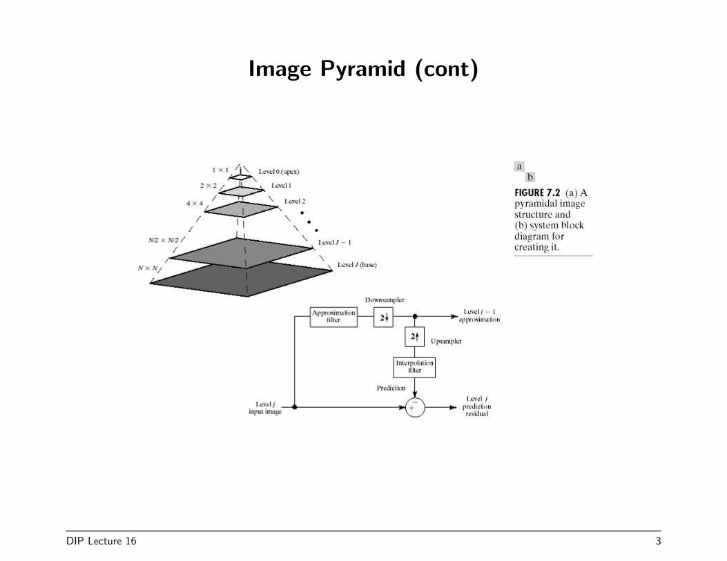
Image Pyramid (cont)

DIP Lecture 16 3

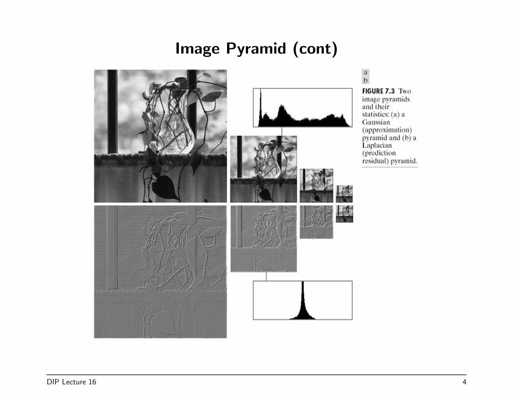
Image Pyramid (cont)

DIP Lecture 16 4

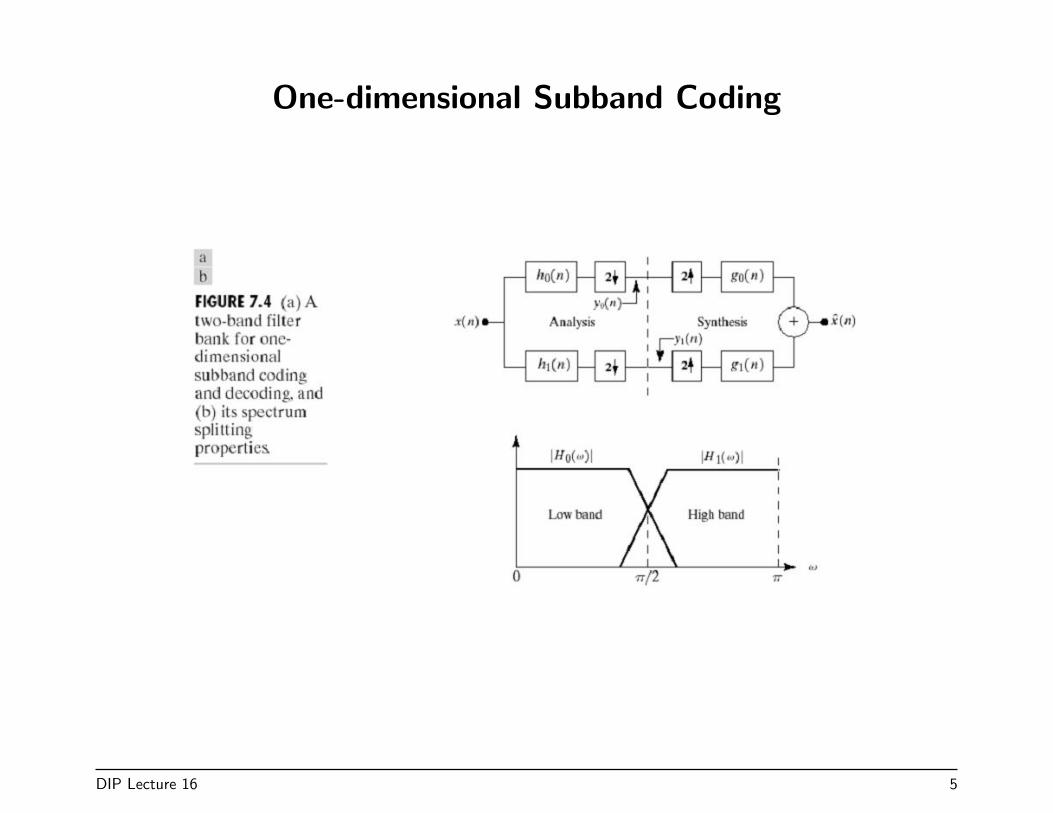
One-dimensional Subband Coding

DIP Lecture 16 5

Subband Coding (cont)

The filters must have certain symmetry properties to enable perfectreconstruction, x(n) = x(n).

Biorthogonal conditions (G&W page 358)

〈hi(2n− k), gj(k)〉 = δ(i− j)δ(n), i, j = {0, 1}

Many filter designs are possible that satisfy these conditions. There is alarge and thorough published literature.

An additional condition, used in development of the fast wavelet transform,is that

〈gi(n), gj(n+ 2m)〉 = δ(i− j)δ(m), i, j = {0, 1}

DIP Lecture 16 6

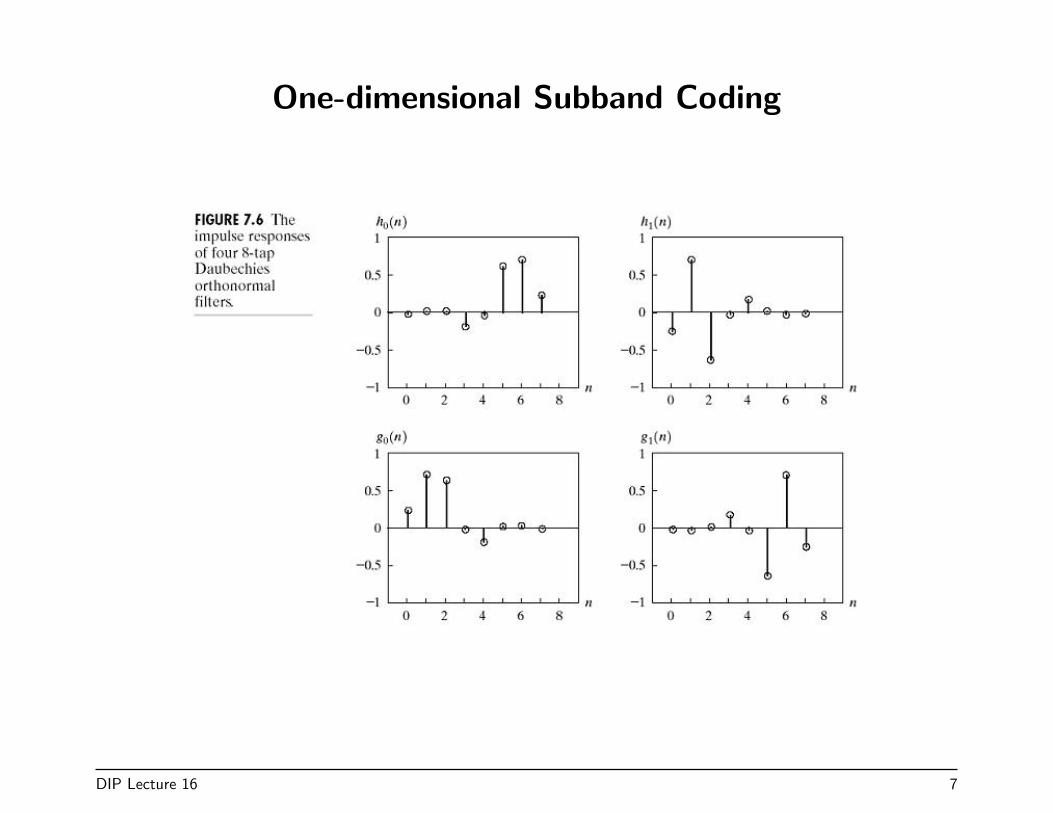
One-dimensional Subband Coding

DIP Lecture 16 7

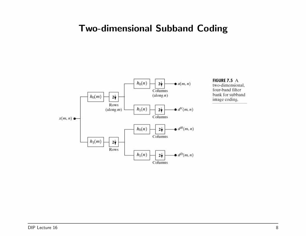
Two-dimensional Subband Coding

DIP Lecture 16 8

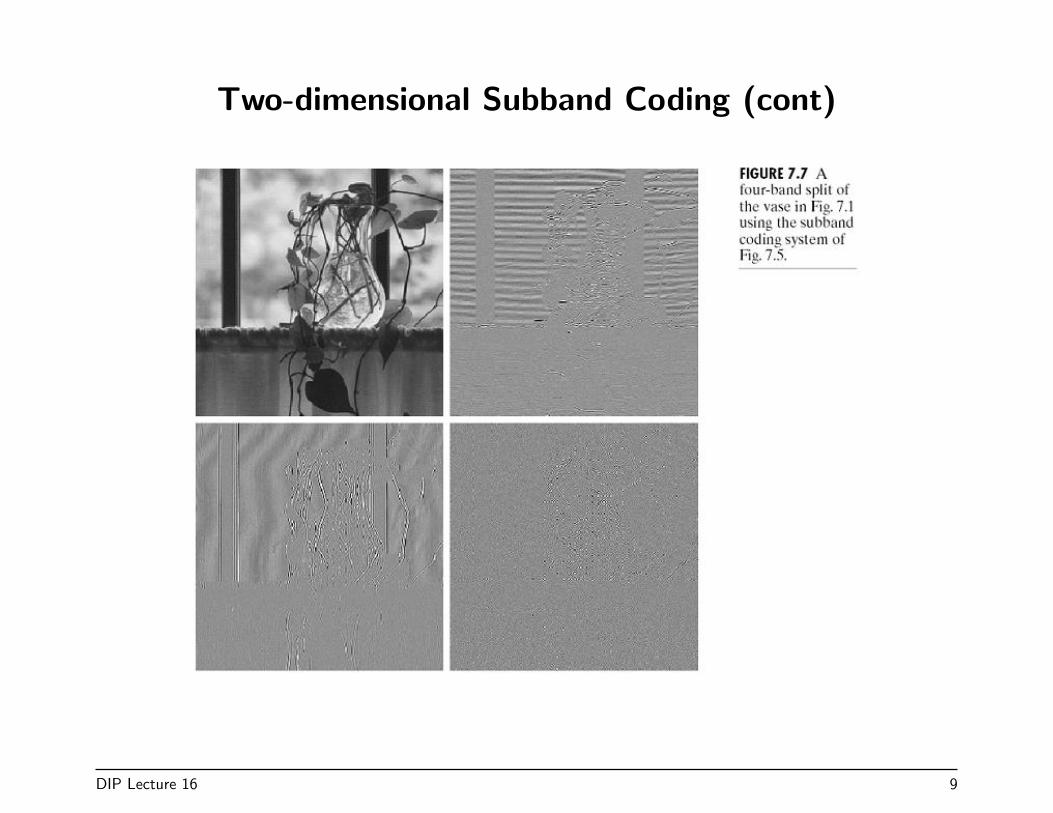
Two-dimensional Subband Coding (cont)

DIP Lecture 16 9

Multiresolution Expansions

In MRA scaling function are used to construct approximations to a function(or an image).

The approximation has 1/2 the number of samples of the original in eachdimension.

Other functions, called wavelets are used to encode the differenceinformation between successive approximations.

We will illustrate the theory with 1D functions and then extend them to2D.

DIP Lecture 16 10

MRA Expansions

A function f(x) can be expanded as

f(x) =∑k

αkϕk(x)

1. The ϕk(x) are real-valued expansion functions.

2. The αk are real-valued expansion coefficients.

3. The set {ϕk(x)} is the basis for a class of functions.

4. The set V = Spank{ϕk(x)} is the set of all functions that can be expressed this way.

V is a vector space.

5. There is a set of dual functions {ϕk(x)} that can be used to compute the coefficients.

αk = 〈ϕk(x), f(x)〉

6. We will show how to construct the set {ϕk(x)} out of scaling functions.

DIP Lecture 16 11

Scaling Functions

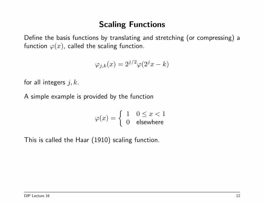
Define the basis functions by translating and stretching (or compressing) afunction ϕ(x), called the scaling function.

ϕj,k(x) = 2j/2ϕ(2jx− k)

for all integers j, k.

A simple example is provided by the function

ϕ(x) ={

1 0 ≤ x < 10 elsewhere

This is called the Haar (1910) scaling function.

DIP Lecture 16 12

Haar Function

DIP Lecture 16 13

Approximation Spaces

The set of scaling functions at any level j can be used to express functionsthat form a set Vj.

f(x) =∑k

αkϕj,k(x)

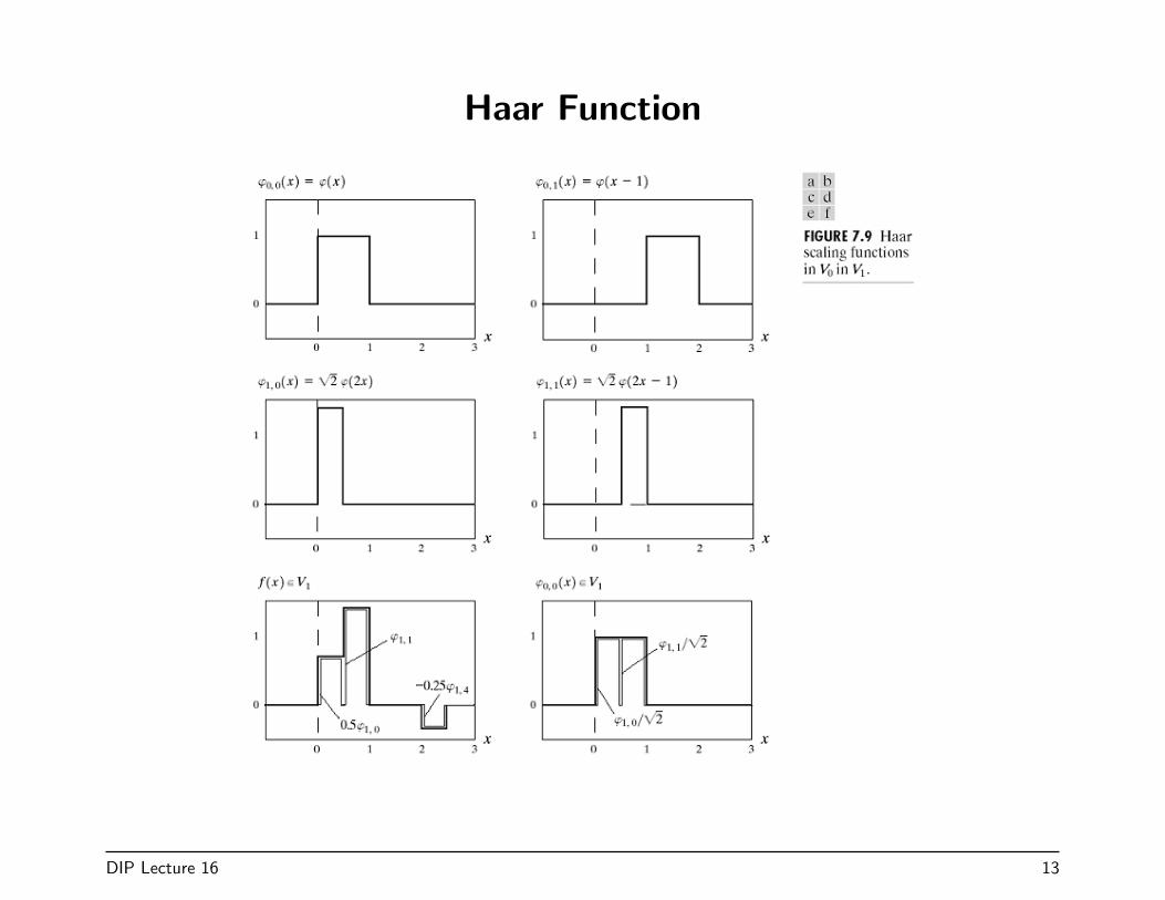
The function

f(x) = 0.5ϕ1,0(x) + ϕ1,1(x)− 0.25ϕ1,4(x)

is shown in Figure 7.9(e) above.

The function ϕ0,k(x) can be expressed as

ϕ0,k(x) =1√2ϕ1,2k(x) +

1√2ϕ1,2k+1(x)

This is illustrated in Figure 7.9(f) above.

DIP Lecture 16 14

Mallat’s Requirements for MRA

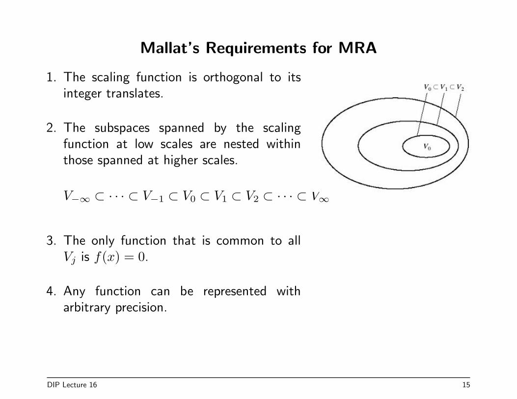
1. The scaling function is orthogonal to itsinteger translates.

2. The subspaces spanned by the scalingfunction at low scales are nested withinthose spanned at higher scales.

V−∞ ⊂ · · · ⊂ V−1 ⊂ V0 ⊂ V1 ⊂ V2 ⊂ · · · ⊂ V∞

3. The only function that is common to allVj is f(x) = 0.

4. Any function can be represented witharbitrary precision.

DIP Lecture 16 15

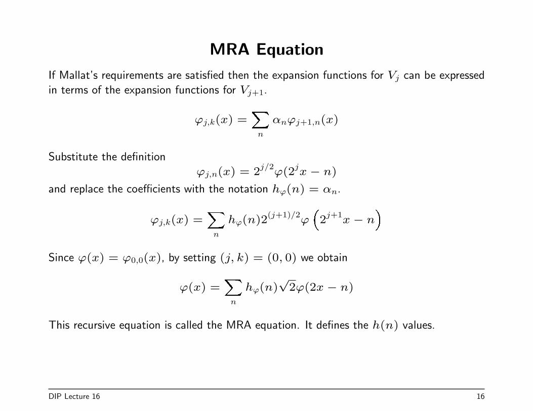
MRA Equation

If Mallat’s requirements are satisfied then the expansion functions for Vj can be expressed

in terms of the expansion functions for Vj+1.

ϕj,k(x) =Xn

αnϕj+1,n(x)

Substitute the definition

ϕj,n(x) = 2j/2ϕ(2

jx− n)

and replace the coefficients with the notation hϕ(n) = αn.

ϕj,k(x) =Xn

hϕ(n)2(j+1)/2

ϕ�2j+1x− n

�

Since ϕ(x) = ϕ0,0(x), by setting (j, k) = (0, 0) we obtain

ϕ(x) =Xn

hϕ(n)√

2ϕ(2x− n)

This recursive equation is called the MRA equation. It defines the h(n) values.

DIP Lecture 16 16

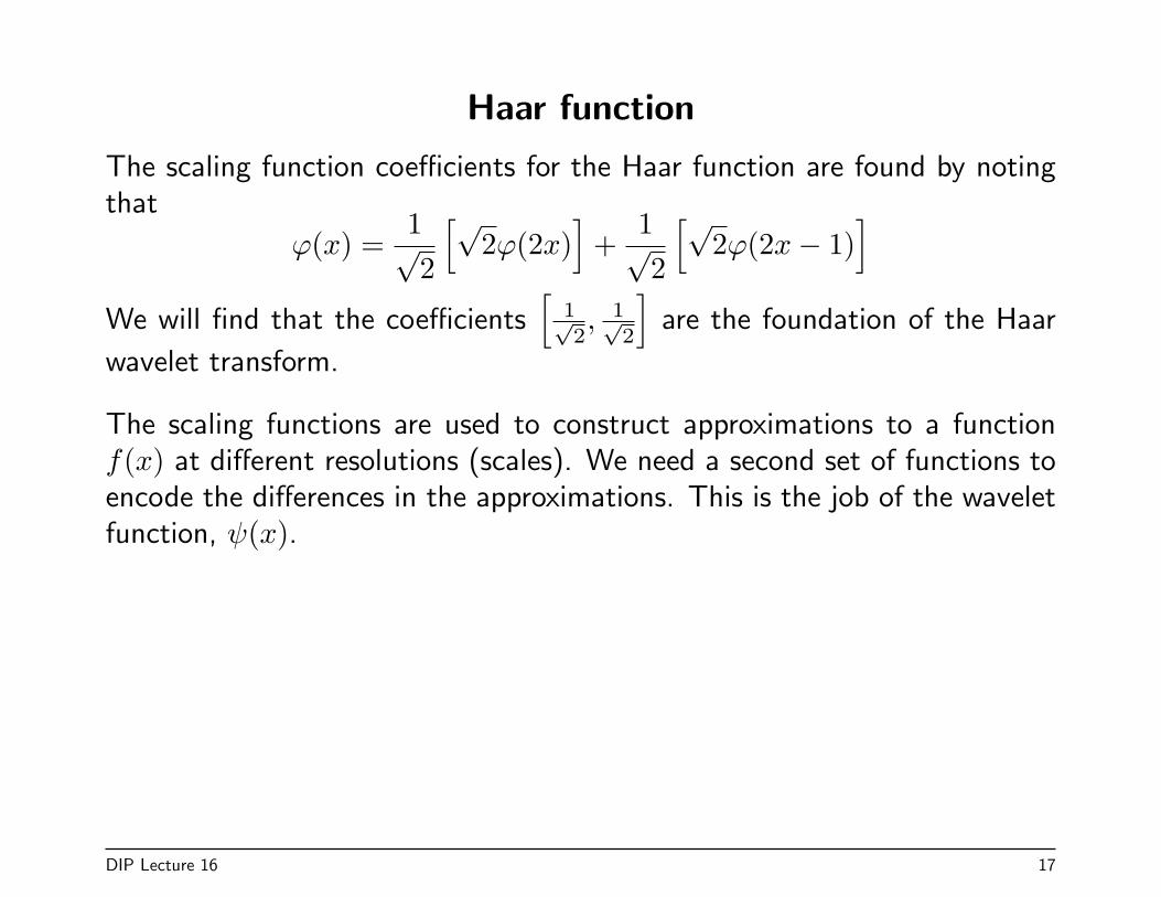
Haar function

The scaling function coefficients for the Haar function are found by notingthat

ϕ(x) =1√2

[√2ϕ(2x)

]+

1√2

[√2ϕ(2x− 1)

]We will find that the coefficients

[1√2, 1√

2

]are the foundation of the Haar

wavelet transform.

The scaling functions are used to construct approximations to a functionf(x) at different resolutions (scales). We need a second set of functions toencode the differences in the approximations. This is the job of the waveletfunction, ψ(x).

DIP Lecture 16 17

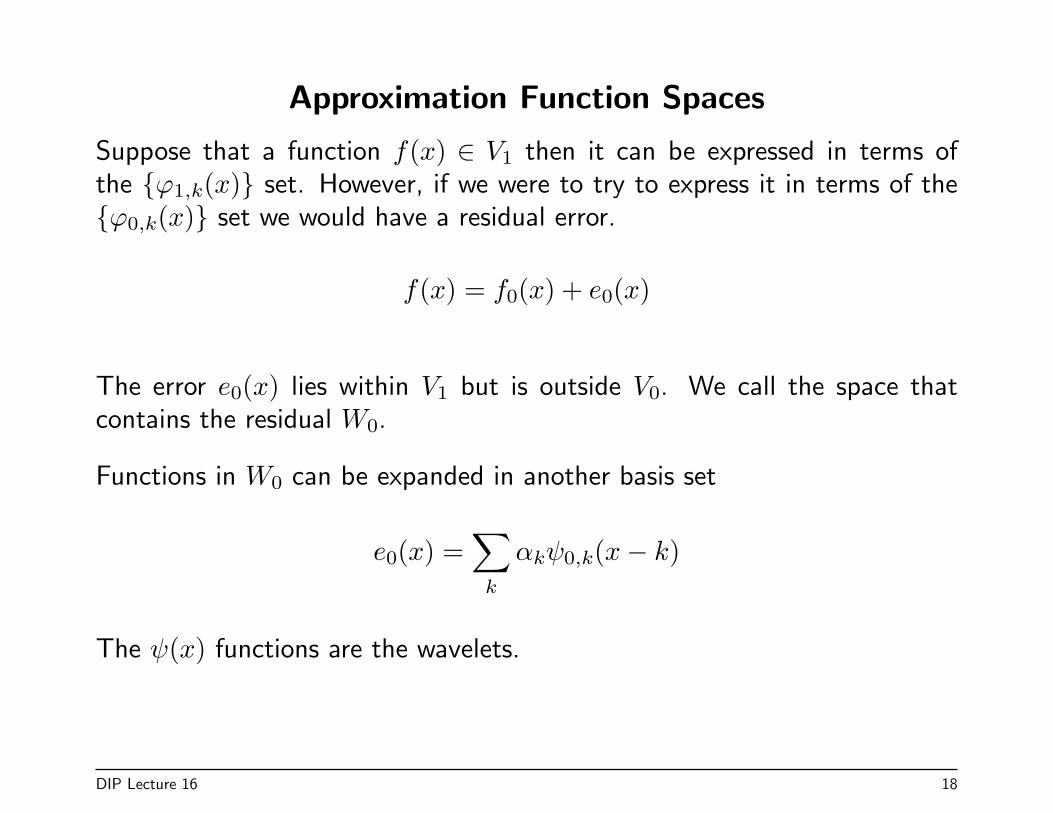
Approximation Function Spaces

Suppose that a function f(x) ∈ V1 then it can be expressed in terms ofthe {ϕ1,k(x)} set. However, if we were to try to express it in terms of the{ϕ0,k(x)} set we would have a residual error.

f(x) = f0(x) + e0(x)

The error e0(x) lies within V1 but is outside V0. We call the space thatcontains the residual W0.

Functions in W0 can be expanded in another basis set

e0(x) =∑k

αkψ0,k(x− k)

The ψ(x) functions are the wavelets.

DIP Lecture 16 18

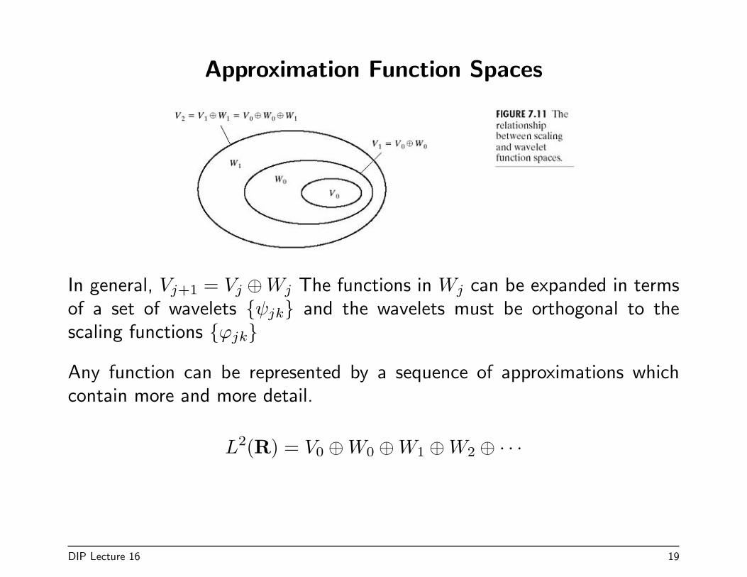
Approximation Function Spaces

In general, Vj+1 = Vj ⊕Wj The functions in Wj can be expanded in termsof a set of wavelets {ψjk} and the wavelets must be orthogonal to thescaling functions {ϕjk}

Any function can be represented by a sequence of approximations whichcontain more and more detail.

L2(R) = V0 ⊕W0 ⊕W1 ⊕W2 ⊕ · · ·

DIP Lecture 16 19

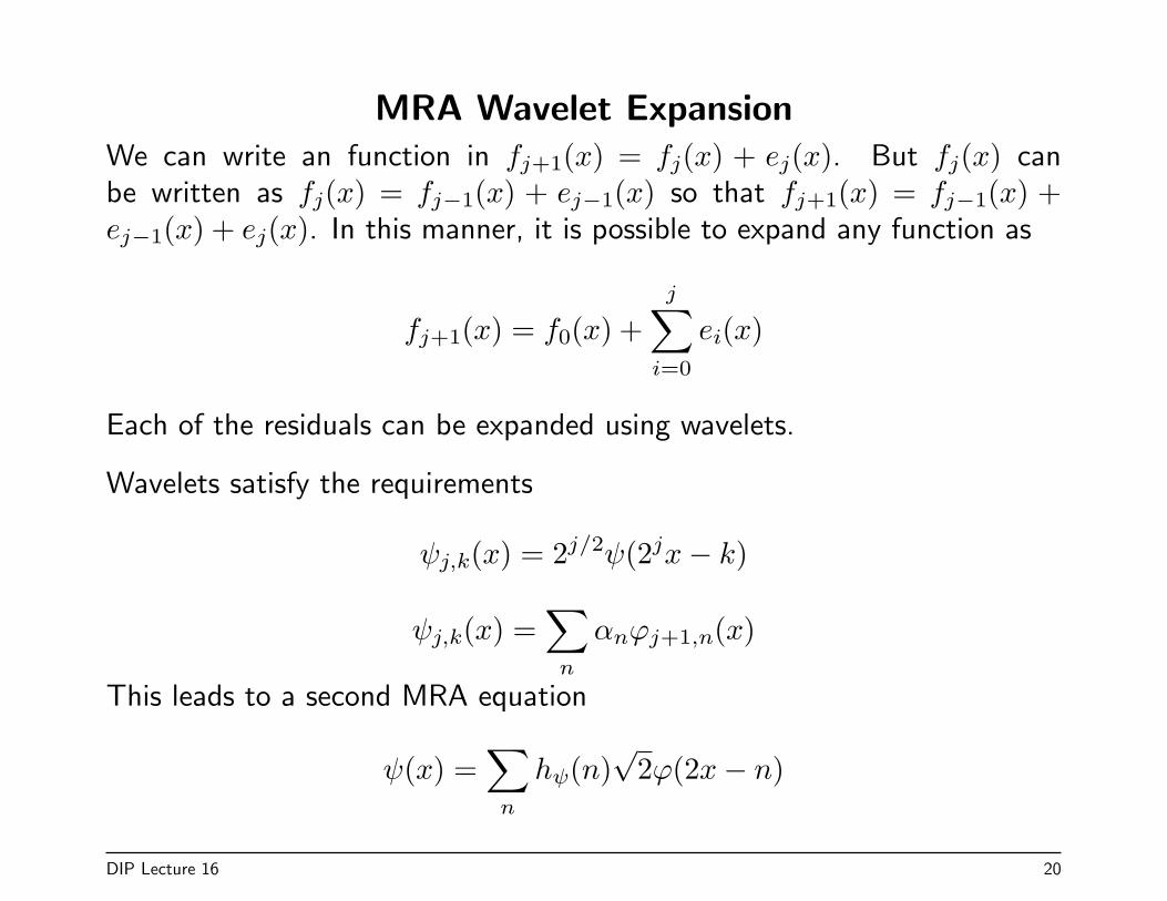
MRA Wavelet ExpansionWe can write an function in fj+1(x) = fj(x) + ej(x). But fj(x) canbe written as fj(x) = fj−1(x) + ej−1(x) so that fj+1(x) = fj−1(x) +ej−1(x) + ej(x). In this manner, it is possible to expand any function as

fj+1(x) = f0(x) +j∑i=0

ei(x)

Each of the residuals can be expanded using wavelets.

Wavelets satisfy the requirements

ψj,k(x) = 2j/2ψ(2jx− k)

ψj,k(x) =∑n

αnϕj+1,n(x)

This leads to a second MRA equation

ψ(x) =∑n

hψ(n)√

2ϕ(2x− n)

DIP Lecture 16 20

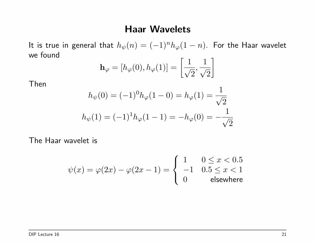
Haar Wavelets

It is true in general that hψ(n) = (−1)nhϕ(1 − n). For the Haar waveletwe found

hϕ = [hϕ(0), hϕ(1)] =[

1√2,

1√2

]Then

hψ(0) = (−1)0hϕ(1− 0) = hϕ(1) =1√2

hψ(1) = (−1)1hϕ(1− 1) = −hϕ(0) = − 1√2

The Haar wavelet is

ψ(x) = ϕ(2x)− ϕ(2x− 1) =

1 0 ≤ x < 0.5−1 0.5 ≤ x < 10 elsewhere

DIP Lecture 16 21

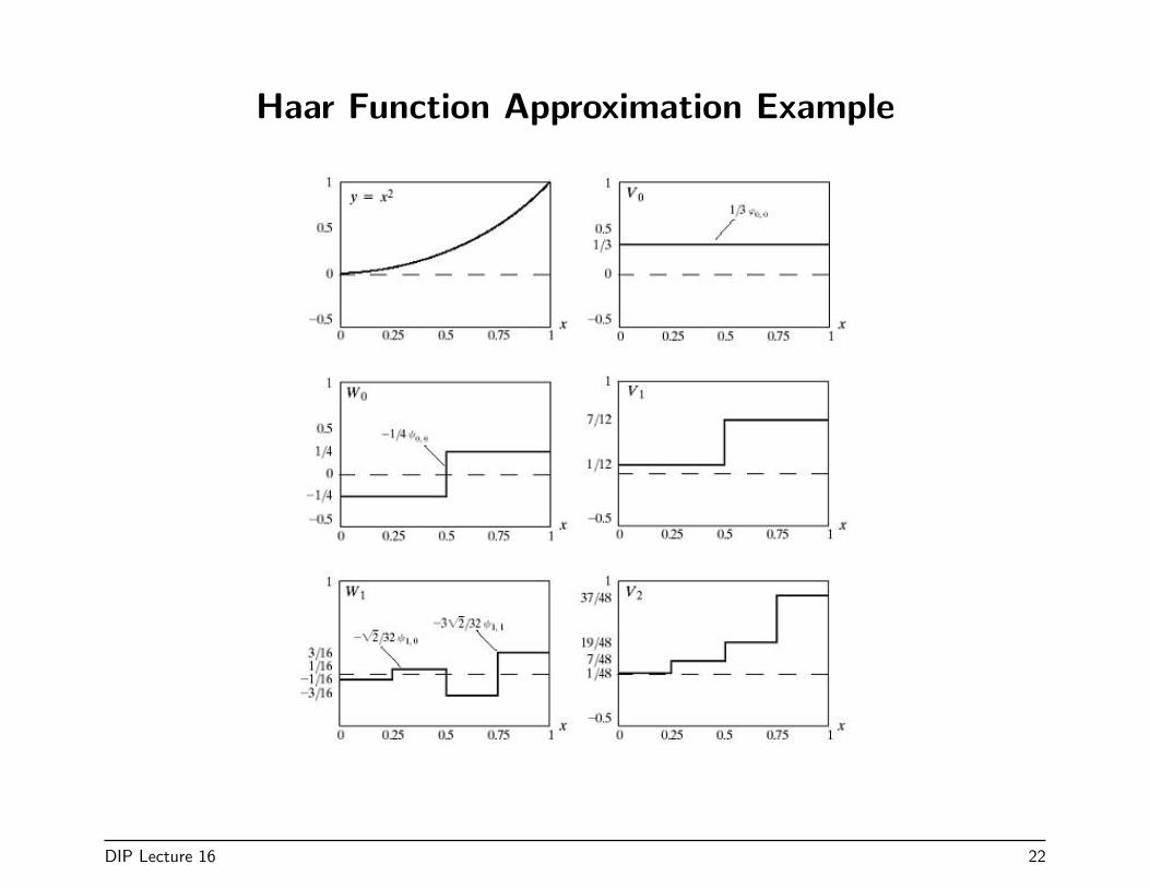
Haar Function Approximation Example

DIP Lecture 16 22

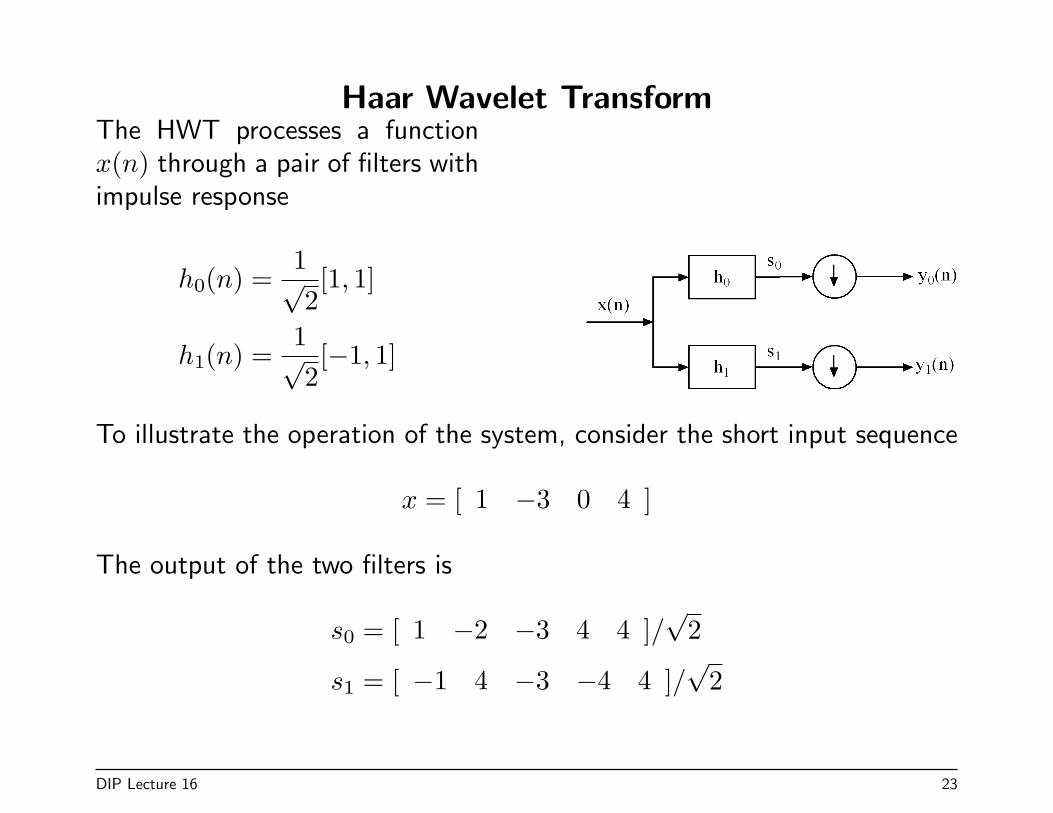
Haar Wavelet TransformThe HWT processes a functionx(n) through a pair of filters withimpulse response

h0(n) =1√2[1, 1]

h1(n) =1√2[−1, 1]

To illustrate the operation of the system, consider the short input sequence

x = [ 1 −3 0 4 ]

The output of the two filters is

s0 = [ 1 −2 −3 4 4 ]/√

2

s1 = [ −1 4 −3 −4 4 ]/√

2

DIP Lecture 16 23

Haar Example (cont)

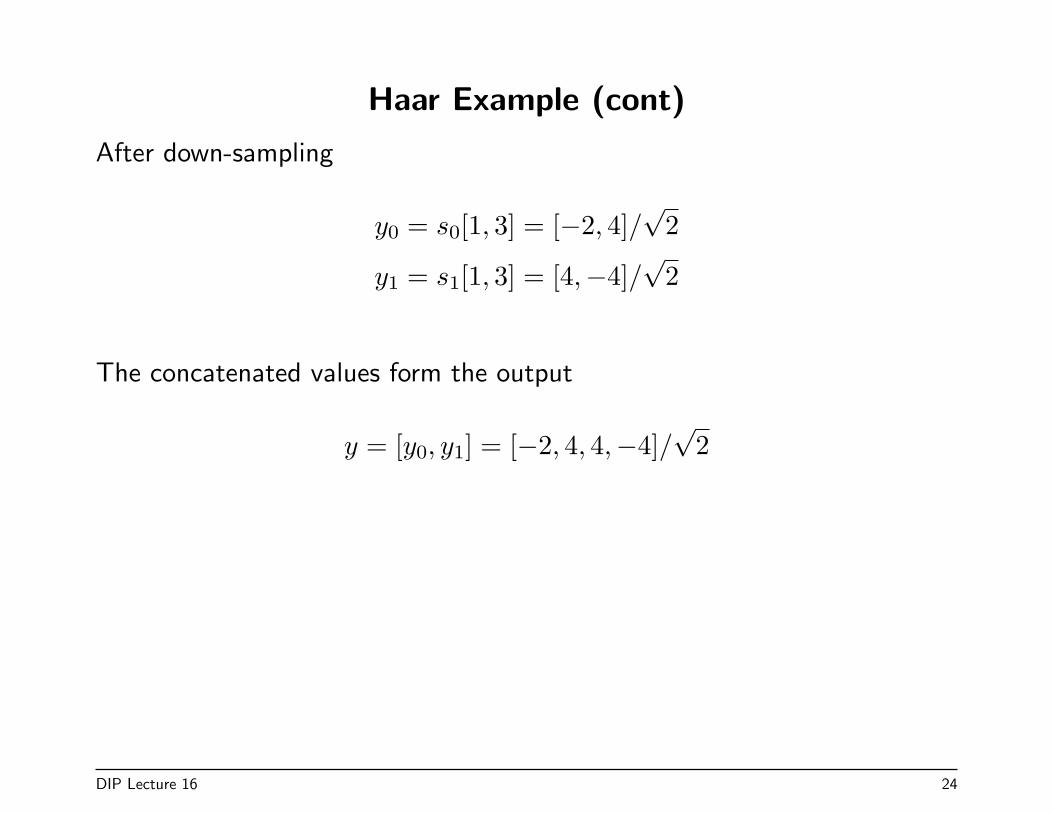
After down-sampling

y0 = s0[1, 3] = [−2, 4]/√

2

y1 = s1[1, 3] = [4,−4]/√

2

The concatenated values form the output

y = [y0, y1] = [−2, 4, 4,−4]/√

2

DIP Lecture 16 24

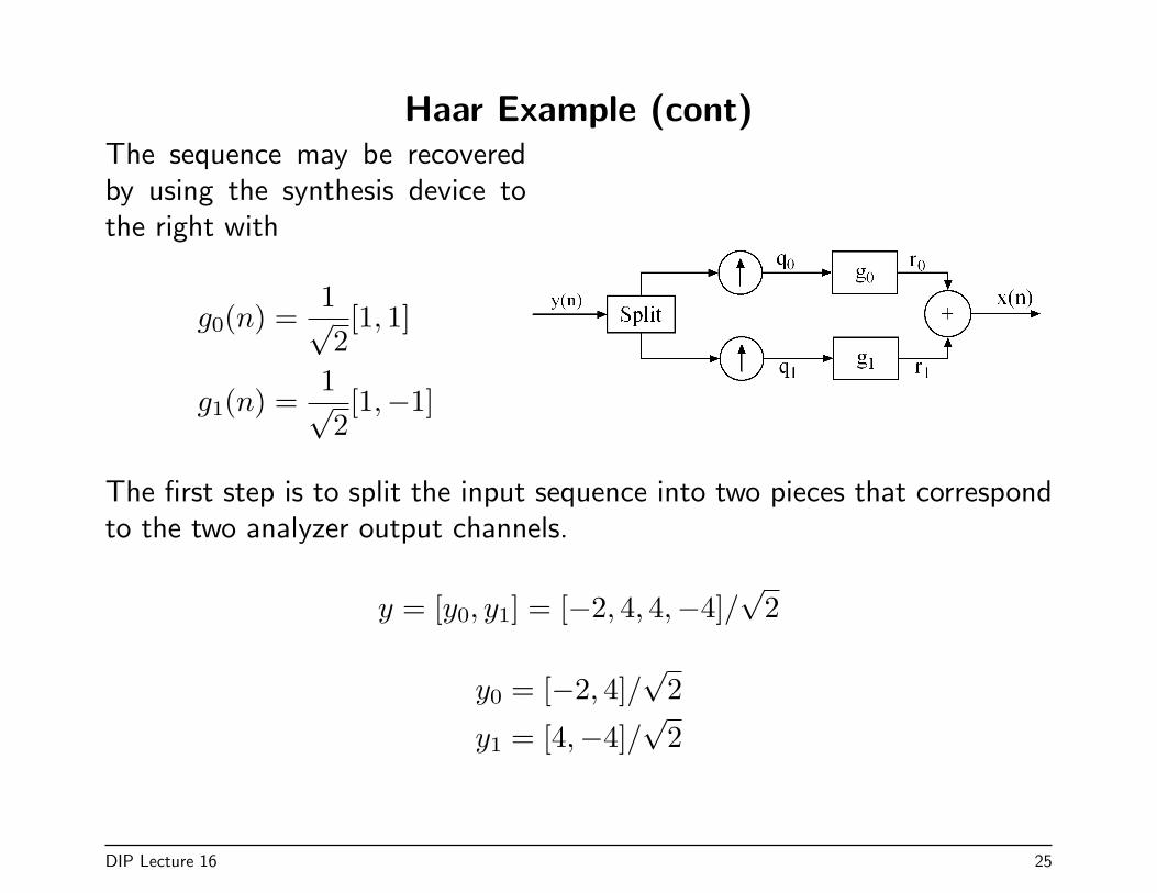
Haar Example (cont)The sequence may be recoveredby using the synthesis device tothe right with

g0(n) =1√2[1, 1]

g1(n) =1√2[1,−1]

The first step is to split the input sequence into two pieces that correspondto the two analyzer output channels.

y = [y0, y1] = [−2, 4, 4,−4]/√

2

y0 = [−2, 4]/√

2

y1 = [4,−4]/√

2

DIP Lecture 16 25

Haar Example (cont)

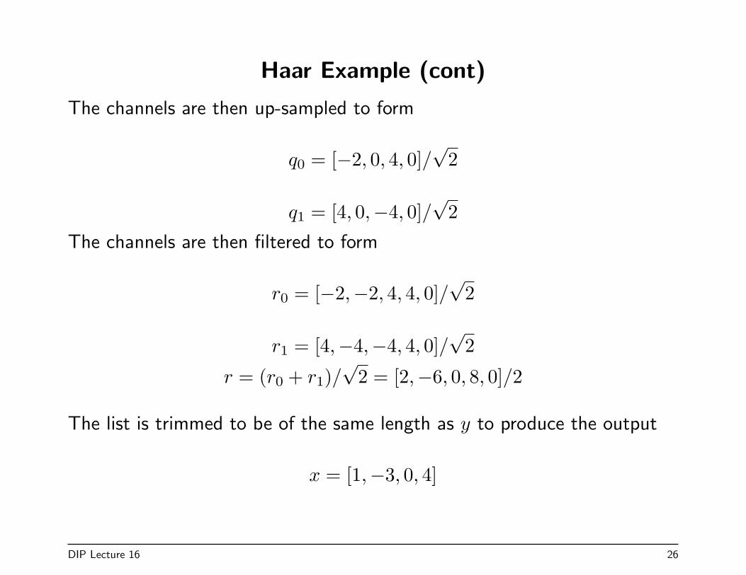
The channels are then up-sampled to form

q0 = [−2, 0, 4, 0]/√

2

q1 = [4, 0,−4, 0]/√

2

The channels are then filtered to form

r0 = [−2,−2, 4, 4, 0]/√

2

r1 = [4,−4,−4, 4, 0]/√

2

r = (r0 + r1)/√

2 = [2,−6, 0, 8, 0]/2

The list is trimmed to be of the same length as y to produce the output

x = [1,−3, 0, 4]

DIP Lecture 16 26

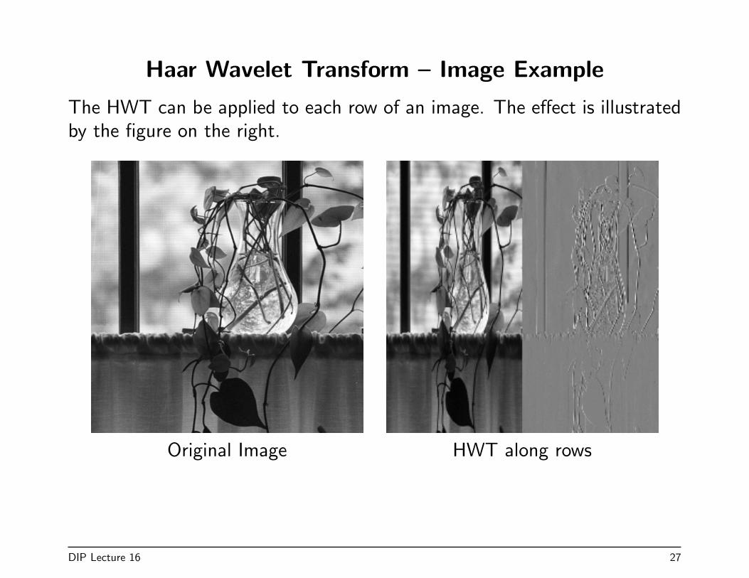
Haar Wavelet Transform – Image Example

The HWT can be applied to each row of an image. The effect is illustratedby the figure on the right.

Original Image HWT along rows

DIP Lecture 16 27

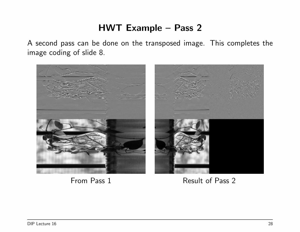
HWT Example – Pass 2

A second pass can be done on the transposed image. This completes theimage coding of slide 8.

From Pass 1 Result of Pass 2

DIP Lecture 16 28

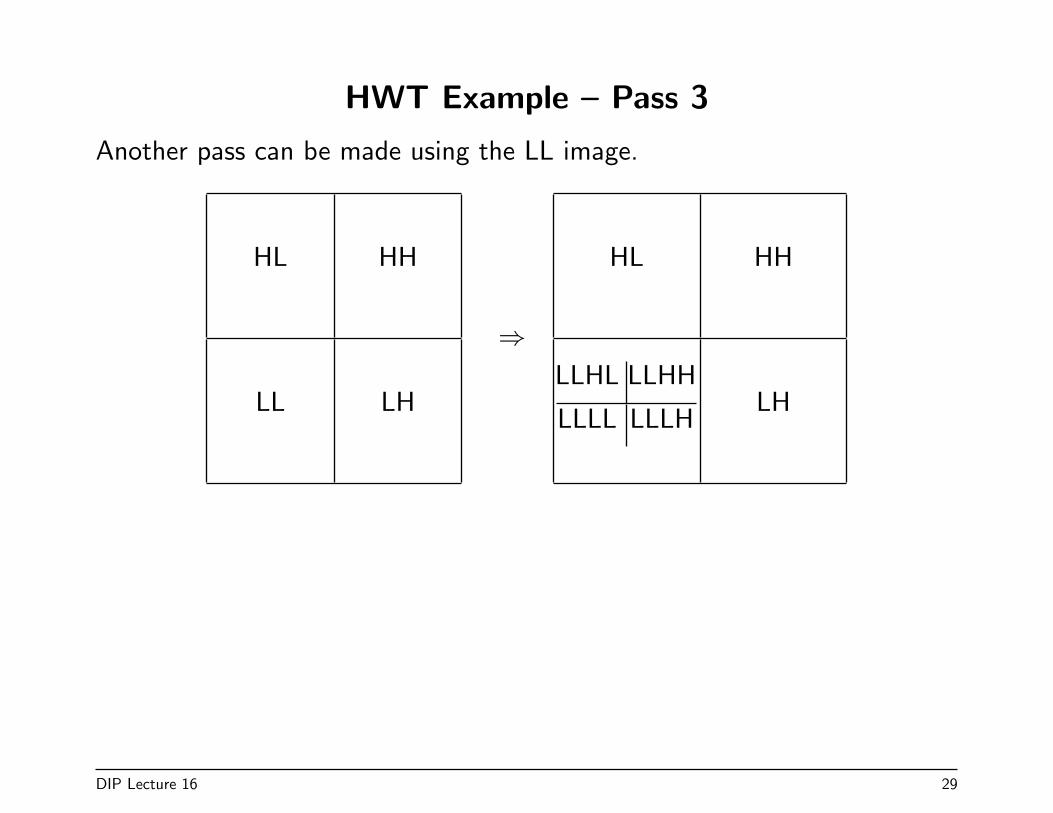
HWT Example – Pass 3

Another pass can be made using the LL image.

HL HH

LL LH

⇒

HL HH

LLHL LLHH

LLLL LLLHLH

DIP Lecture 16 29

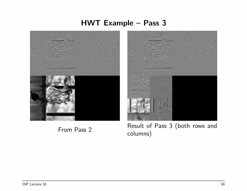
HWT Example – Pass 3

From Pass 2Result of Pass 3 (both rows andcolumns)

DIP Lecture 16 30