Lecture 24 : Review of Math 320 Linear Algebra and ...ywang/teaching/Ma320_s18/Lecture...Math 320 Linear Algebra and Diﬀerential Equations Spring 2018, UW-Madison 1 Core concepts

Math 320 Linear Algebra and Differential Equations Spring 2018, UW-Madison

Lecture 24 : Review of Math 320

Linear Algebra and Differential Equations

• What have we learned in this course?

Please read the Preface of the textbook to get the big picture aboutwhat we have learned in the past three months.

Roughly speaking, we have covered more than half of the contents

in the following two courses:

– Math 319: Techniques in Ordinary Differential Equation;

– Math 340: Elementary Matrices and Linear Algebra.

All of you did great jobs during the whole semester. Congratula-tions!

• What can you do in the future?

– If you are interested in Differential Equations, you can choose:

∗ More proofs: Math 519: Ordinary Differential Equations,Math 322: Applied Mathematical Analysis ;

∗ More applications: Math 415: Applied Dynamical Systems,Chaos and Modeling.

– If you are interested in Linear Algebra, you have lots of choices:

∗ More proofs: Math 341: Linear Algebra;

∗ More applications: Math 443: Applied Linear Algebra, Math

513: Numerical Linear Algebra, Math 525: Linear Program-ming Methods.

1 Copy right reserved by Yingwei Wang


1 Core concepts in linear algebra

1.1 Basic matrix operations

The notation Am×n = (ai,j)1≤i≤m,1≤j≤n means the matrix A has m rows and n columns,and its each entry is denoted by ai,j , where the row index i goes from 1 to m and columnindex j goes from 1 to n.

If m = n, then we say A is a square matrix.The basic operations of matrices are shown as follows.

• Scalar-matrix multiplication. For any constant k ∈ R, we have

kAm×n := (kai,j)1≤i≤m,1≤j≤n.

• Matrix-matrix addition. For two matrices with the same size, e.g.,Am×n = (ai,j)1≤i≤m,1≤j≤n

and Bm×n = (bi,j)1≤i≤m,1≤j≤n, we have

A+B := (ai,j + bi,j)1≤i≤m,1≤j≤n.

• Matrix-vector muliplication. For matrix A and vector v, we have

Am×nvn×1 = um×1, (1.1)

where each entry in vector u is given by ui =∑n

j=1 ai,jvj.

• Matrix-matrix muliplication.

Am×nBn×p = Cm×p. (1.2)

Each entry of Cm×p = (ci,j)1≤i≤m,1≤j≤p is the dot product of i-th row of A andj-th column of B, i.e., ci,j =

∑n

k=1 ai,kbk,j.

⋆ ∗ The number of columns in A should be exactly the same as the number ofrows in B. Otherwise, the matrix-matrix product does not make sense!!! Thisleads to the following property:

AB 6= BA; (1.3)

Some remarks on (1.3).

∗Everything marked ⋆ means you have to know it very well.



1. The “ 6=” may refer to the matrix sizes or the values.

2. For scalar k and identity matrix I, the following identities hold for any squarematrix A,

(kI)A = A(kI) = kA.

• The inverse of a matrix. The (multiplicative) inverse of a square matrix A,denoted as A−1, is defined by the following

AA−1 = I, A

−1A = I, (1.4)

where I is the identity matrix. If A−1 exists, then we say A is invertible.

For a 2-by-2 matrix A, its inverse can be found easily:

A =

[

a b

c d

]

, A−1 =

1

ad− bc

[

d −b

−c a

]

. (1.5)

For the 3-by-3 matrices, we have to use other technical methods.

1.2 Linear dependence and linear independence

Consider a finite nonempty set S = {v1,v2, · · · ,vk} in a “vector space”V, and constants{c1, c2, · · · , ck}, and this equation

c1v1 + c2v2 + · · · ckvk = 0. (1.6)

1. If there exists at least one cj 6= 0 such that (1.6) holds, then we say the vectors{v1,v2, · · · ,vk} are linearly dependent.

2. If the only possible values are c1 = c2 = · · · = ck = 0 , then we say the vectors{v1,v2, · · · ,vk} are linearly independent.

Remark 1.1. Here are several important concepts related to linear dependence andlinear independence:

1. An expression of the form c1v1+ c2v2+ · · · ckvk is called a linear combination

of the vectors {v1,v2, · · · ,vk}.

2. A set of vectors S = {vj}kj=1 ⊂ V is called a basis set for a vector space V if

(a) All of the vectors in S are linearly independent;



(b) V = span {vj}kj=1.(i.e. every vector in V can be written as a linear combi-

nation of the vectors in S.)

3. The dimension of a vector space means the numnber of linearly independentvectors (the number of entries in the basis set) in this spcace.

4. If the vectors {v1,v2, · · · ,vk} are the columns (or rows) of a matrix A, then themaximum number of linearly independent vectors in S is the rank of this matrix.

1.3 ⋆ Summary of singular or nonsingular matrices

Suppose A is an n× n square matrix. The following statements are equivalent to eachother:

1. A is nonsingular ;

2. A is invertible (i.e. ∃A−1 such that AA−1 = A

−1A = In);

3. det(A) 6= 0;

4. There are no “zero rows”after Gaussian Eliminations;

5. A is row equivalent to In;

6. The nonhomogeneous equation Ax = b has unique solution for any right handside b;

7. The homogeneous equation Ax = 0 has only trivial solution (zero solution);

8. The nullspace of A is {0};

9. The column (row) vectors of A are linearly independent (i.e. they form a basisfor Rn) and Col(A) = Row(A) = R

n;

10. Rank(A) = dim(Col(A)) = dim(Row(A)) = n;

11. AT is nonsingular (invertible);

12. All of the eigenvalues of A are nonzero.

Similarly, the following statements are also equivalent to each other:

1. A is singular ;



2. A is non-invertible;

3. det(A) = 0;

4. There are at least one “zero row”after Gaussian Elimination;

5. A is not row equivalent to In;

6. The nonhomogeneous equation Ax = b has either infinitely many solution or nosolution;

7. The homogeneous equation Ax = 0 has non trivial solutions (nonzero solutions);

8. ∃x 6= 0, s.t. x ∈ Null(A);

9. The column (row) vectors of A are linearly dependent ;

10. Rank(A) = dim(Col(A)) = dim(Row(A)) < n;

11. AT is singular (non-invertible);

12. At least one of the eigenvalues of A is zero.

1.4 Subspace

Given a vector space V , let W be a non-empty subset of V , denoted as W ⊂ V . Inother words, for every w ∈ W , we have w ∈ V .

Furthermore, if W itself is a vector space, it is called a subspace of V .Quesion: How to check whether W is a subspace of V or not?

(0) 0 ∈ W ;

(1) v +w ∈ W ;

(2) cv ∈ W .

In other words, the subspace W should is “closed” under addition v + w andmultiplication cv.

The rules (1) and (2) can be combined into a single requirement: the rule forsubspaces: A subspace containing v andw must contain all linear combinations cv+dw.

Several examples:



1. R1 is a subspace of R2;

2. R1 is a subspace of R3;

3. R2 is a subspace of R3.

1.5 More general vector spaces (other than Rn)

• Matrix space: All of 2-by-2 matrices, i.e.,

M2 =

{

A =

(

a b

c d

)

, a, b, c, d ∈ R

}

.

1. Basis set:

{(

1 00 0

)

,

(

0 10 0

)

,

(

0 01 0

)

,

(

0 00 1

)}

.

2. Dimension: dim(M2) = 4.

• Polynomial space: All polynomials with degree ≤ 2, i.e.,

P2 ={

p(x) = a + bx+ cx2, a, b, c ∈ R}

.

1. Basis set: {1, x, x2}.

2. Dimension: dim(P2) = 3.

Several examples of subspaces:

1. An example for the subspace of matrix spaceM2 is {all of the 2-by-2 matrix has zero trace},i.e.,

M02 =

{

A =

(

a11 a12a21 a22

)

: a11 + a22 = 0

}

⊂ M2.

2. An example for the subspace of the polynomial space P2 is P1, i.e.,

P1 = {p(x) = a + bx, a, b ∈ R} ⊂ P2.



1.6 ⋆ Four fundamental subspaces of a matrix

Consider a matrix Am×n. The four fundamental subspaces of A are as follows:

1. Column space: Col(A) = {all linear combinations of the columns of A} is a sub-space of Rm and dim(Col(A)) = rank(A);

2. Row space: Col(AT ) = {all linear combinations of the rows of A} is a subspaceof Rn and dim(Col(AT )) = rank(A);

3. Null space: Null(A) = {all solutions to Ax = 0} is a subspace ofRn and dim(Null(A)) =n− rank(A);

4. Leftnull space: Null(AT ) ={

all solutions to ATx = 0

}

is a subspace of Rm and

dim(Null(AT )) = m− rank(A).

5. Both row space and null space are subspaces of Rn and they are orthogonal toeach other, i.e.,

Null(A) ⊥ Row(A), dim(Null(A)) + dim(Row(A)) = n.

6. Both column space and leftnull space are subspaces of Rm and they are orthogonalto each other, i.e.,

Null(AT ) ⊥ Col(A), dim(Null(AT )) + dim(Col(A)) = m.

1.7 Eigenvalues and eigenvectors

The relation between the eigenvalues and eigenvectors is

Avj = λjvj.

Useful properties of eigenvalues and eigenvectors:

1. The product of the n eigenvalues of A is the same as the determinant of A, i.e.,

Πnk=1 = λ1λ2 · · ·λn = det(A).

2. The sum of the n eigenvalues of A is the same as the trace of A, i.e.,

n∑

k=1

λk =

n∑

k=1

akk.



3. A set of eigenvectors of A, each corresponding to a different eigenvalue of A, is alinearly independent set.

4. If λ is an eigenvalue of A, then the dimension of eigenspace Eλ = Null(A− λI),which is called the geometric multiplicity, is at most the algebraic multiplicity ofλ.

5. Let P (λ) = det(A−λI) be the characteristic polynomial of A. Then the Cayley-Hamilton Theorem says that P (A) = 0.

6. A andAT have the same eigenvalues but different eigenvectors. Note that det(A−

λI) = det(AT − λI).

7. The eigenvalues of 2A,A2 and A+ 2I are respectively,

(a) 2A has eigenvalues {2λk}nk=1;

(b) A2 has eigenvalues {λ2

k}nk=1;

(c) A+ 2I has eigenvalues {λk + 2}nk=1.

8. Suppose A is invertible and has eigenvalue λ and eigenvector v. Then A−1 has

eigenvalue λ−1 and eigenvector v.

2 Useful skills in linear algebra

2.1 ⋆ Find the determinant of a matrix

We have learned three basic methods to find the determinant of a matrix:

1. By the definition of determinant.

2. Perform cofactor expansion along a row or a column.

3. Use elementary row (column) operations to simplify a determinant( i.e. to makethe matrix to be a lower (upper) triangular matrix).

Remark 2.1. There are several important properties of the determinants:

det(AT ) = det(A),

det(ApB

q) = (det(A))p(det(B))q,



det(A−1) =1

det(A),

det(αA) = αn det(A).

More uesful properties:

• Triangular. If A is upper/lower triangular matrix, then det(A) is the productof the diagonal entries.

• Zero row or column. If one row/column of A is zero, then det(A) = 0.

• Duplicate rows or columns. If two rows/columns are identical, then det(A) =0.

• In general, det(A + B) 6= det(A) + det(B). For instant, A =

(

1 00 0

)

,B =(

0 00 1

)

, then det(A) = det(B) = 0 but det(A+B) = 1.

Remark 2.2. The determinant has many applications in this course. Here are someof them:

1. Determine a square matrix is singular or not;

2. Determine the columns / rows of a square matrix are linearly dependent or linearlyindependent;

3. Cramer’s rule to solve a linear system;

4. Adjoint method to find the inverse of a matrix;

5. Find the eigenvalues of a matrix;

6. Use Wronskian determinant to show the linear independence of several functionsand application in variation of parameter method to find a particular solution.

Hence, it is extremely important for you to know how to find the determinants forboth 2-by-2 and 3-by-3 matrices.



2.2 Find the inverse of a matrix

We have already learned two methods to find the inverse of a matrix A:

1. ⋆ Gauss-Jordan elimination:

[A | I] → [B | P ] → [I | A−1],

⇒ PA = B,

⇒ A = P−1B.

2. Adjoint method :

A−1 =

1

det(A)adj (A), (2.1)

adj (A) = Cofactor(A)T . (2.2)

Do not forget the transpose in the definition of adj(A).

Remark 2.3. No matter what method you use, please make sure the correctness ofyour results by checking AA

−1 = A−1A = I.

Remark 2.4. There are several important properties about the inverse:

(A−1)−1 = A,

(AB)−1 = B−1A

−1,

(AT )−1 = (A−1)T .

2.3 Solve the linear system Ax = b

2.3.1 If Ax = b has unique solution

We have already learned two methods to solve the linear system Ax = b:

1. Perform Gaussian elimination to the augmented matrix A# = [A | b].

2. Cramer’s rule.

Remark 2.5. No matter what method you use, please make sure the correctness ofyour results by checking Ax = b.



2.3.2 If Ax = b has infinitely many solutions

⋆ There are two steps to find the complete solution to Ax = b:

1. Find all linearly independent null solutions to Axn = 0.

2. Find one particular solution xp satifying Axp = b.

Then the the complete solution is x = xn + xp.

Remark 2.6. Let us make a summary about the relation between the coefficients of thesystem of equations and its solutions. Suppose after elementary row operations, we getthe augmented matrix like

A# =

1 ∗ ∗ | ∗0 1 ∗ | ∗0 0 p | q

.

Then we can conclude that

1. it has no solution if p = 0, q 6= 0;

2. it has infinitely many solutions if p = 0, q = 0;

3. it has unique solution if p 6= 0, ∀q.

2.4 ⋆ Find the base for Null(A)

Solve the linear system Ax = 0 and find all the linearly independent solutions.

The applications of finding the null space of a matrix:

1. Solve the homogeneous linear system Axn = 0.

2. Find the eigenvectors (A− λI)v = 0.

2.5 ⋆ Find the base for Col(A)

There are three ways:

1. Perform the Gaussian elimination on [A | b] and find the requirement for baccording to Remark 2.6.

2. Perform Gaussian elimination on AT to get the row reduced echelon form.

3. Perform Gaussian elimination on A and figure out which columns of the originalmatrices are the bases.



2.6 ⋆ Find eigenvalues and eigenvectors

There are two steps to find the eigenvalues and eigenvectors of a matrix A:

1. Step One: to find the roots of the characteristic polynomial:

p(λ) = det(A− λI) = 0. (2.3)

The roots {λj}nj=1 are called eigenvalues of A.

2. Step Two: to find the basis of Null(A − λjI), i.e., to find linearly independentsolutions to the linear system

(A− λjI)vj = 0, ∀j. (2.4)

The solutions to (2.4) are denoted as {vj}nj=1, which are called eigenvectors of

A.

2.7 Diagonalization of a matrix

Suppose n-by-n matrix A = (aij)ni,j=1 has n eigenvalues (including each according to

its multiplicity) {λk}nk=1 and n linearly independent eigenvectors {vk}

nk=1. Let Λ be a

diagonal matrix with {λk}nk=1 as diagonal entries and V be the matrix with {vk}

nk=1 as

the columns. Then the matrix A can be written as

A = V ΛV−1. (2.5)

1. The n-by-n matrix A is diagonalizable if and only if A has n independenteigenvectors.

2. The n-by-n matrix A is diagonalizable if and only if for each eigenvalue λ, itsgeometric multiplicity is the same as its algebraic multiplicity.

A typical example for nondiagonalizable is A =

(

1 10 1

)

.

⋆ One of the benefits of the form (2.5) is that it provides an efficient way to computethe powers and exponentials of A.

Ak = V Λk

V−1, (2.6)

eA = V eΛV −1, (2.7)



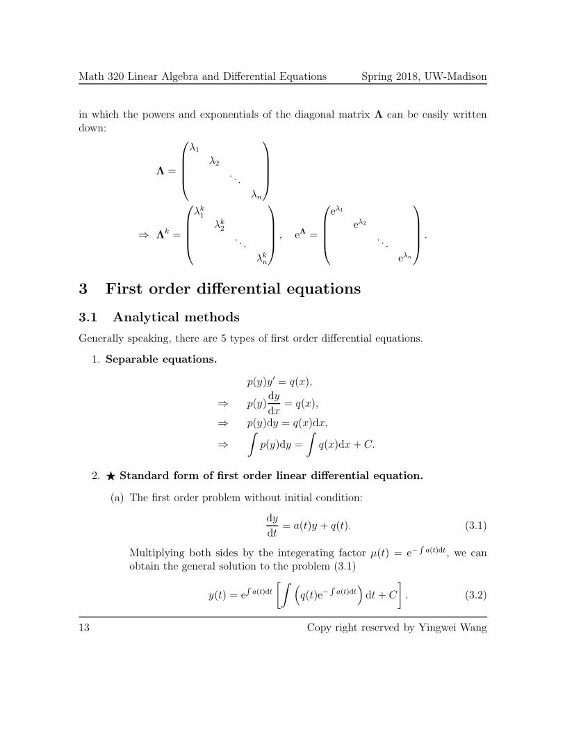
in which the powers and exponentials of the diagonal matrix Λ can be easily writtendown:

Λ =

λ1

λ2

. . .

λn

⇒ Λk =

λk1

λk2

. . .

λkn

, eΛ =

eλ1

eλ2

. . .

eλn

.

3 First order differential equations

3.1 Analytical methods

Generally speaking, there are 5 types of first order differential equations.

1. Separable equations.

p(y)y′ = q(x),

⇒ p(y)dy

dx= q(x),

⇒ p(y)dy = q(x)dx,

⇒

∫

p(y)dy =

∫

q(x)dx+ C.

2. ⋆ Standard form of first order linear differential equation.

(a) The first order problem without initial condition:

dy

dt= a(t)y + q(t). (3.1)

Multiplying both sides by the integerating factor µ(t) = e−∫a(t)dt, we can

obtain the general solution to the problem (3.1)

y(t) = e∫a(t)dt

[∫

(

q(t)e−∫a(t)dt

)

dt + C

]

. (3.2)



(b) The first order problem with initial condition at t = 0:

{

dydt

= a(t)y + q(t),y(0) = y0.

(3.3)

The unique solution to the problem (3.3) is

y(t) = e∫ t

0a(s)dsy0 +

∫ t

0

q(s)e∫ t

sa(τ)dτds. (3.4)

Let us define the growth factor G(s, t) as follows:

G(s, t) = e∫ t

sa(τ)dτ . (3.5)

Then the equation (3.4) becomes

y(t) = G(0, t)y0 +

∫ t

0

q(s)G(s, t)ds. (3.6)

(c) The first order problem with initial condition at t = t0:

{

dydt

= a(t)y + q(t),y(t0) = y0.

(3.7)

The solution is

y(t) = G(t0, t)y0 +

∫ t

t0

q(s)G(s, t)ds. (3.8)

3. Homogeneous equation. The homogeneous equation looks like y′ = f(x, y)where f(tx, ty) = f(x, y). The technique here is to make the change of variablesy = xv(x) and to reduce the problem to a separable equation. Note that

y = xv(x),

⇒ dy = vdx+ xdv, (by product rule)

⇒dy

dx= v + x

dv

dx.

4. Bernoulli equation. The general form of the Bernoulli equation

dy

dx+ p(x)y = q(x)yn. (3.9)



By changing of variablesu(x) = y(x)1−n,

the Eq. (3.9) becomes

du

dx+ (1− n)p(x)u = (1− n)q(x). (3.10)

We can use the formula (3.1)-(3.2) to solve Eq.(3.10).

5. Exact equation. The exact equation is in this form:

M(x, y)dx+N(x, y)dy = 0, (3.11)

where M(x, y) and N(x, y) satisfy

My = Nx.

The general procedure to solve the exact equation is as follows: Starting from∂F (x,y)

∂x= M(x, y), we can get

F (x, y) =

∫

M(x, y)dx

= g(x, y) +B(y).

It implies that∂F (x, y)

∂y=

∂g(x, y)

∂y+B′(y).

On the other hand, we know that

∂F (x, y)

∂y= N(x, y).

We can solve B(y) and then the solution is F (x, y) = C.

3.2 Uniqueness and Stability analysis

Theorem 3.1 (Existence and uniqueness of the solution). Consider the first orderinitial value problem

dy

dt= f(t, y), (3.12)



y(a) = b. (3.13)

If the 2D functions f(t, y) and ∂f(t,y)∂y

are continuous on some rectangle R in the ty-

plane containing the point (a, b), Then a solution exists and is unique on some intervalI containing the point t = a.

See Theorem 1 on page 23 of your textbook.

Recall that an equilibrium solution (also called “critical point” or “steadystate”) is any constant (horizontal) function y(t) = c that is a solution to the differentialequation.

Consider the autonomous equation:

dy(t)

dt= F (y), y > 0, t > 0. (3.14)

The definitions of stable, unstale, semistable equilibrium solutions to (3.14) areas follows:

Stable: The equilibrium solution y(t) = c is stable if all solutions with initial conditionsy0 ‘near’ y = c approach c as t → ∞.

Unstable: The equilibrium solution y(t) = c is unstable if all solutions with initial condi-tions y0 ‘near’ y = c do NOT approach c as t → ∞.

Semistable: The equilibrium solution y(t) = c is semistable if initial conditions y0 on oneside of c lead to solutions y(t) that approach c as t → ∞, while initial conditionsy0 on the other side of c do NOT approach c.

⋆ Consider the autonomous equation (3.14), in which F (y) and dFdy

are continuous.How to find all of its equilibrium solutions and classify they are stable or unstable?

1. Solve F (y) = 0 to get the equilibrium solutions (critical points).

2. Study F (y) around the equilibrium values as follows (drawing the phase dia-gram: F (y) vs y might help)

(a) Draw a vertical line (the phase line) and make tick marks at equilibriumvalues.

(b) Between tick marks determine if F (y) is positive or negative.



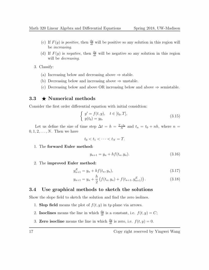
(c) If F (y) is positive, then dydt

will be positive so any solution in this region willbe increasing.

(d) If F (y) is negative, then dydt

will be negative so any solution in this regionwill be decreasing.

3. Classify:

(a) Increasing below and decreasing above ⇒ stable.

(b) Decreasing below and increasing above ⇒ unstable.

(c) Decreasing below and above OR increasing below and above ⇒ semistable.

3.3 ⋆ Numerical methods

Consider the first order differential equation with initial considtion:{

y′ = f(t, y), t ∈ [t0, T ],y(t0) = y0,

(3.15)

Let us define the size of time step ∆t = h = T−t0N

and tn = t0 + nh, where n =0, 1, 2, . . . , N . Then we have

t0 < t1 < · · · < tN = T.

1. The forward Euler method:

yn+1 = yn + hf(tn, yn). (3.16)

2. The improved Euler method:

yEn+1 = yn + hf(tn, yn), (3.17)

yn+1 = yn +h

2

(

f(tn, yn) + f(tn+1, yEn+1)

)

. (3.18)

3.4 Use graphical methods to sketch the solutions

Show the slope field to sketch the solution and find the zero isolines.

1. Slop field means the plot of f(t, y) in ty-plane via arrows.

2. Isoclines means the line in which dydt

is a constant, i.e. f(t, y) = C;

3. Zero isocline means the line in which dydt

is zero, i.e. f(t, y) = 0.



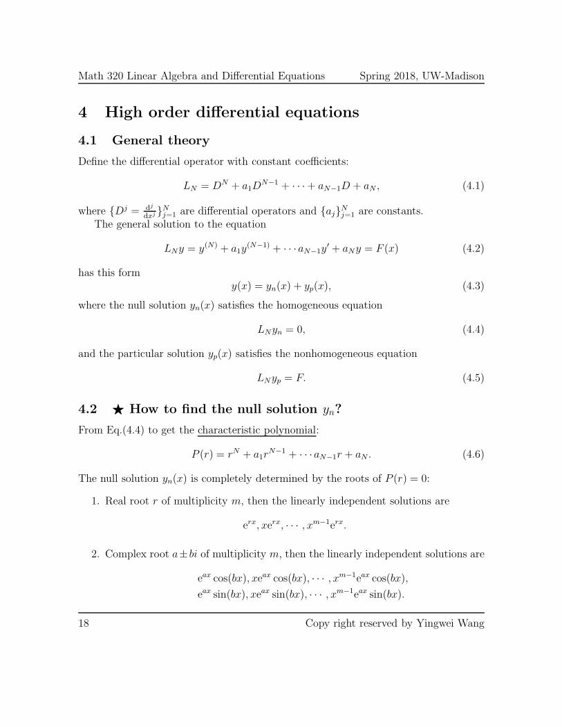
4 High order differential equations

4.1 General theory

Define the differential operator with constant coefficients:

LN = DN + a1DN−1 + · · ·+ aN−1D + aN , (4.1)

where {Dj = dj

dxj }Nj=1 are differential operators and {aj}

Nj=1 are constants.

The general solution to the equation

LNy = y(N) + a1y(N−1) + · · · aN−1y

′ + aNy = F (x) (4.2)

has this formy(x) = yn(x) + yp(x), (4.3)

where the null solution yn(x) satisfies the homogeneous equation

LNyn = 0, (4.4)

and the particular solution yp(x) satisfies the nonhomogeneous equation

LNyp = F. (4.5)

4.2 ⋆ How to find the null solution yn?

From Eq.(4.4) to get the characteristic polynomial:

P (r) = rN + a1rN−1 + · · ·aN−1r + aN . (4.6)

The null solution yn(x) is completely determined by the roots of P (r) = 0:

1. Real root r of multiplicity m, then the linearly independent solutions are

erx, xerx, · · · , xm−1erx.

2. Complex root a± bi of multiplicity m, then the linearly independent solutions are

eax cos(bx), xeax cos(bx), · · · , xm−1eax cos(bx),

eax sin(bx), xeax sin(bx), · · · , xm−1eax sin(bx).



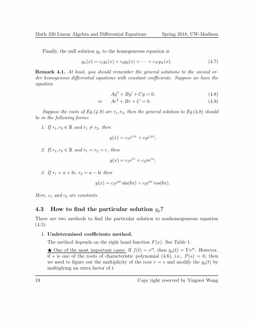
Finally, the null solution yn to the homogeneous equation is

yn(x) = c1y1(x) + c2y2(x) + · · ·+ cNyN(x). (4.7)

Remark 4.1. At least, you should remember the general solutions to the second or-der homogenous differential equations with constant coefficients. Suppose we have theequation

Ay′′ +By′ + Cy = 0, (4.8)

⇒ Ar2 +Br + C = 0. (4.9)

Suppose the roots of Eq.(4.9) are r1, r2, then the general solution to Eq.(4.8) shouldbe in the following forms:

1. If r1, r2 ∈ R and r1 6= r2, then

y(x) = c1er1x + c2e

r2x;

2. If r1, r2 ∈ R and r1 = r2 = r, then

y(x) = c1erx + c2xe

rx;

3. If r1 = a + bi, r2 = a− bi then

y(x) = c1eax sin(bx) + c2e

ax cos(bx).

Here, c1 and c2 are constants.

4.3 How to find the particular solution yp?

There are two methods to find the particular solution to nonhomogeneous equation(4.5):

1. Undetermined coefficients method.

The method depends on the right hand function F (x). See Table 1.

⋆ One of the most important cases: If f(t) = est, then yp(t) = Y est. However,if s is one of the roots of characteristic polynomial (4.6), i.e., P (s) = 0, thenwe need to figure out the multiplicity of the root r = s and modify the yp(t) bymultiplying an extra factor of t.



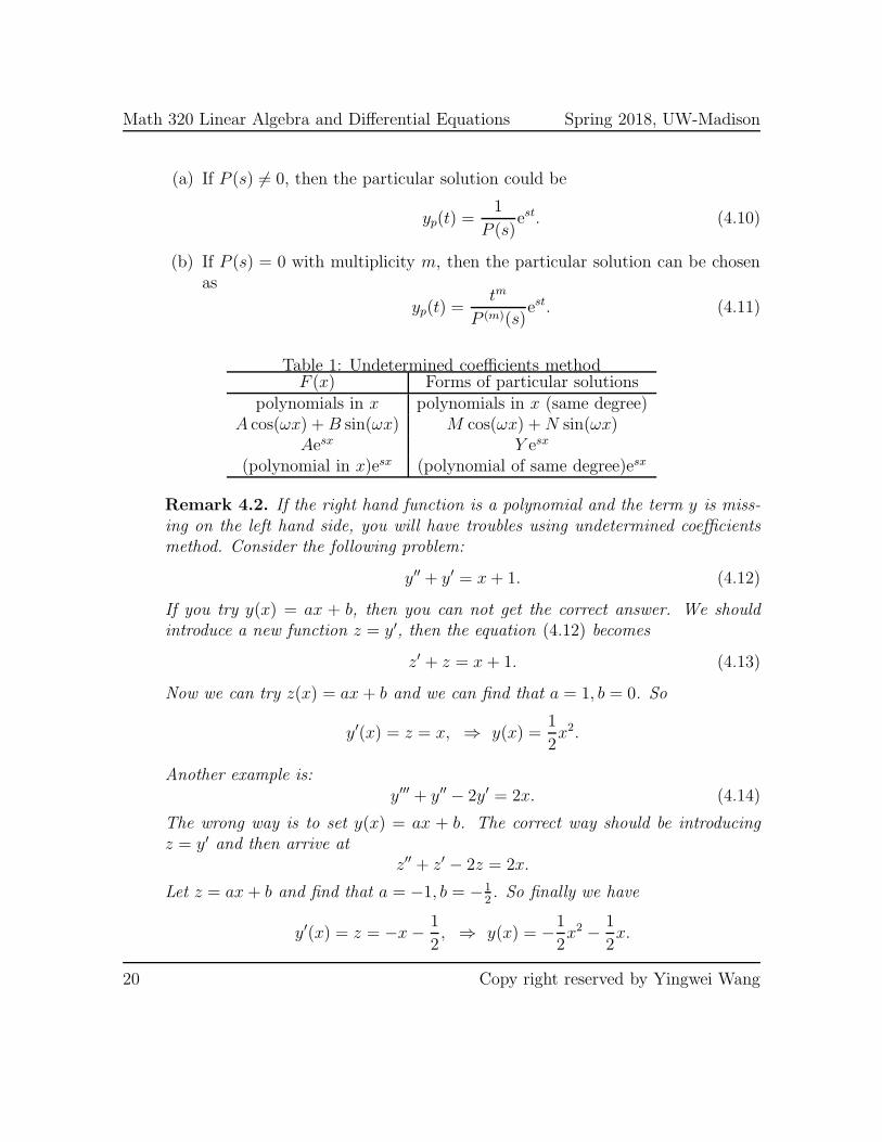
(a) If P (s) 6= 0, then the particular solution could be

yp(t) =1

P (s)est. (4.10)

(b) If P (s) = 0 with multiplicity m, then the particular solution can be chosenas

yp(t) =tm

P (m)(s)est. (4.11)

Table 1: Undetermined coefficients methodF (x) Forms of particular solutions

polynomials in x polynomials in x (same degree)A cos(ωx) +B sin(ωx) M cos(ωx) +N sin(ωx)

Aesx Y esx

(polynomial in x)esx (polynomial of same degree)esx

Remark 4.2. If the right hand function is a polynomial and the term y is miss-ing on the left hand side, you will have troubles using undetermined coefficientsmethod. Consider the following problem:

y′′ + y′ = x+ 1. (4.12)

If you try y(x) = ax + b, then you can not get the correct answer. We shouldintroduce a new function z = y′, then the equation (4.12) becomes

z′ + z = x+ 1. (4.13)

Now we can try z(x) = ax+ b and we can find that a = 1, b = 0. So

y′(x) = z = x, ⇒ y(x) =1

2x2.

Another example is:y′′′ + y′′ − 2y′ = 2x. (4.14)

The wrong way is to set y(x) = ax + b. The correct way should be introducingz = y′ and then arrive at

z′′ + z′ − 2z = 2x.

Let z = ax+ b and find that a = −1, b = −12. So finally we have

y′(x) = z = −x−1

2, ⇒ y(x) = −

1

2x2 −

1

2x.



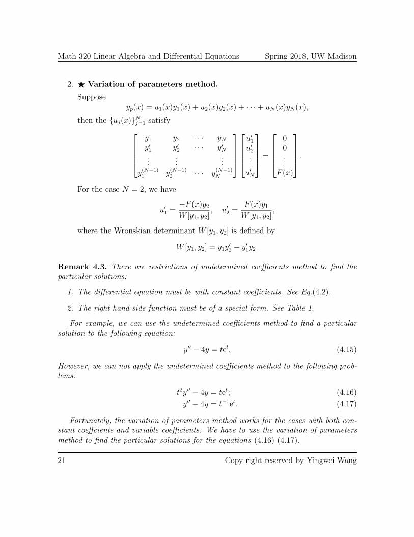
2. ⋆ Variation of parameters method.

Supposeyp(x) = u1(x)y1(x) + u2(x)y2(x) + · · ·+ uN(x)yN(x),

then the {uj(x)}Nj=1 satisfy

y1 y2 · · · yNy′1 y′2 · · · y′N...

......

y(N−1)1 y

(N−1)2 · · · y

(N−1)N

u′1

u′2...

u′N

=

00...

F (x)

.

For the case N = 2, we have

u′1 =

−F (x)y2W [y1, y2]

, u′2 =

F (x)y1W [y1, y2]

,

where the Wronskian determinant W [y1, y2] is defined by

W [y1, y2] = y1y′2 − y′1y2.

Remark 4.3. There are restrictions of undetermined coefficients method to find theparticular solutions:

1. The differential equation must be with constant coefficients. See Eq.(4.2).

2. The right hand side function must be of a special form. See Table 1.

For example, we can use the undetermined coefficients method to find a particularsolution to the following equation:

y′′ − 4y = tet. (4.15)

However, we can not apply the undetermined coefficients method to the following prob-lems:

t2y′′ − 4y = tet; (4.16)

y′′ − 4y = t−1et. (4.17)

Fortunately, the variation of parameters method works for the cases with both con-stant coeffcients and variable coefficients. We have to use the variation of parametersmethod to find the particular solutions for the equations (4.16)-(4.17).



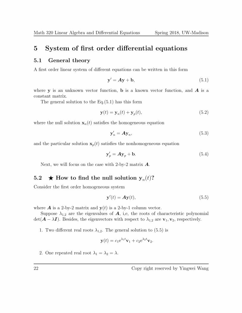
5 System of first order differential equations

5.1 General theory

A first order linear system of different equations can be written in this form

y′ = Ay + b, (5.1)

where y is an unknown vector function, b is a known vector function, and A is aconstant matrix.

The general solution to the Eq.(5.1) has this form

y(t) = yn(t) + yp(t), (5.2)

where the null solution xn(t) satisfies the homogeneous equation

y′n = Ayn, (5.3)

and the particular solution xp(t) satisfies the nonhomogeneous equation

y′p = Ayp + b. (5.4)

Next, we will focus on the case with 2-by-2 matrix A.

5.2 ⋆ How to find the null solution yn(t)?

Consider the first order homogeneous system

y′(t) = Ay(t), (5.5)

where A is a 2-by-2 matrix and y(t) is a 2-by-1 column vector.Suppose λ1,2 are the eigenvalues of A, i,e, the roots of characteristic polynomial

det(A− λI). Besides, the eigenvectors with respect to λ1,2 are v1,v2, respectively.

1. Two different real roots λ1,2. The general solution to (5.5) is

y(t) = c1eλ1tv1 + c2e

λ2tv2.

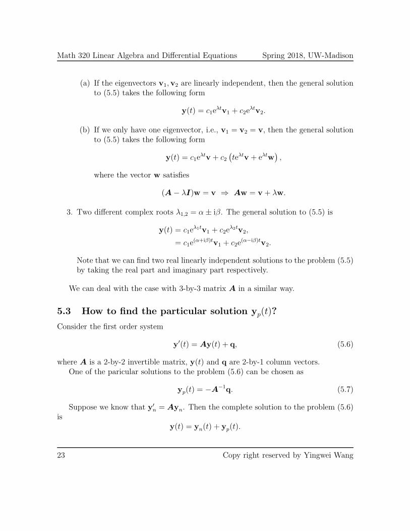
2. One repeated real root λ1 = λ2 = λ.



(a) If the eigenvectors v1,v2 are linearly independent, then the general solutionto (5.5) takes the following form

y(t) = c1eλtv1 + c2e

λtv2.

(b) If we only have one eigenvector, i.e., v1 = v2 = v, then the general solutionto (5.5) takes the following form

y(t) = c1eλtv + c2

(

teλtv + eλtw)

,

where the vector w satisfies

(A− λI)w = v ⇒ Aw = v + λw.

3. Two different complex roots λ1,2 = α± iβ. The general solution to (5.5) is

y(t) = c1eλ1tv1 + c2e

λ2tv2,

= c1e(α+iβ)tv1 + c2e

(α−iβ)tv2.

Note that we can find two real linearly independent solutions to the problem (5.5)by taking the real part and imaginary part respectively.

We can deal with the case with 3-by-3 matrix A in a similar way.

5.3 How to find the particular solution yp(t)?

Consider the first order system

y′(t) = Ay(t) + q, (5.6)

where A is a 2-by-2 invertible matrix, y(t) and q are 2-by-1 column vectors.One of the paricular solutions to the problem (5.6) can be chosen as

yp(t) = −A−1q. (5.7)

Suppose we know that y′n = Ayn. Then the complete solution to the problem (5.6)

isy(t) = yn(t) + yp(t).


Documents

Lecture 24 : Review of Math 320 Linear Algebra and ...ywang/teaching/Ma320_s18/Lecture...Math 320 Linear Algebra and Diﬀerential Equations Spring 2018, UW-Madison 1 Core concepts