Embed Size (px)
Citation preview
Lecture 3 Iterative methods for solving linear system
Weinan E1,2 and Tiejun Li2
1Department of Mathematics,
Princeton University,
2School of Mathematical Sciences,
Peking University,
No.1 Science Building, 1575

Outline
Iterations
I Iterative methods
Object: construct sequence {xk}∞k=1, such that xk converge to a fixed
vector x∗, and x∗ is the solution of the linear system.
I General iteration idea:
If we want to solve equations
g(x) = 0,
and the equation x = f(x) has the same solution as it, then construct
xk+1 = f(xk).
If xk → x∗, then x∗ = f(x∗), thus the root of g(x) is obtained.
Matrix form for Jacobi iterations
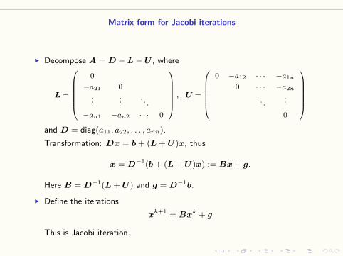
I Decompose A = D −L−U , where
L =
0
−a21 0
......
. . .
−an1 −an2 · · · 0
, U =
0 −a12 · · · −a1n
0 · · · −a2n
. . ....
0
and D = diag(a11, a22, . . . , ann).
Transformation: Dx = b + (L + U)x, thus
x = D−1(b + (L + U)x) := Bx + g.
Here B = D−1(L + U) and g = D−1b.
I Define the iterations
xk+1 = Bxk + g
This is Jacobi iteration.
Component form of Jacobi iterations
I Jacobi iterations
xk+11 =
(b1 −
∑j 6=1
a1jxkj
)/a11
xk+12 =
(b2 −
∑j 6=2
a2jxkj
)/a22
· · · · · · · · ·
xk+1n =
(bn −
∑j 6=n
anjxkj
)/ann
I Update each component of xk according to each equation simultaneously
and independently by freezing the other variables at former step.
I Parallel in nature!
Jacobi iterations
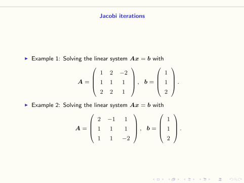
I Example 1: Solving the linear system Ax = b with
A =
1 2 −2
1 1 1
2 2 1
, b =
1
1
2
.
I Example 2: Solving the linear system Ax = b with
A =
2 −1 1
1 1 1
1 1 −2
, b =
1
1
2
.
Jacobi iterations
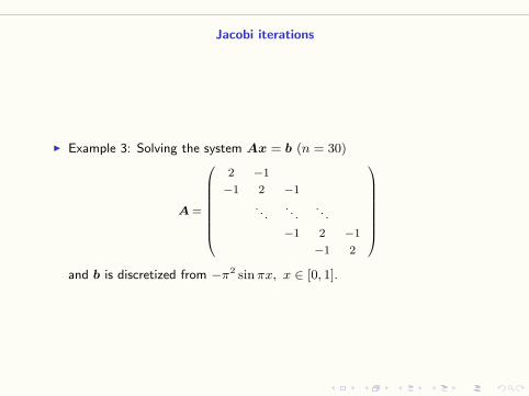
I Example 3: Solving the system Ax = b (n = 30)
A =
2 −1
−1 2 −1
. . .. . .
. . .
−1 2 −1
−1 2
and b is discretized from −π2 sinπx, x ∈ [0, 1].
Jacobi iterations
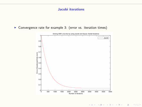
I Convergence rate for example 3: (error vs. iteration times)
0 500 1000 1500 2000 2500 3000 3500 4000 4500 50000
0.1
0.2
0.3
0.4
0.5
0.6
0.7
0.8
0.9
1
Number of iterations
Err
or o
f ite
ratio
ns(in
finite
nor
m)
Solving ODE u’(x)=f(x) by using Jacobi and Gauss−Seidel iterations
Jacobi
Gauss-Seidel iterations
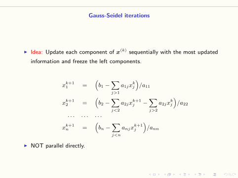
I Idea: Update each component of x(k) sequentially with the most updated
information and freeze the left components.
xk+11 =
(b1 −
∑j>1
a1jxkj
)/a11
xk+12 =
(b2 −
∑j<2
a2jxk+1j −
∑j>2
a2jxkj
)/a22
· · · · · · · · ·
xk+1n =
(bn −
∑j<n
anjxk+1j
)/ann
I NOT parallel directly.
Matrix form for Gauss-Seidel iteration
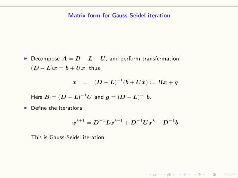
I Decompose A = D −L−U , and perform transformation
(D −L)x = b + Ux, thus
x = (D −L)−1(b + Ux) := Bx + g
Here B = (D −L)−1U and g = (D −L)−1b.
I Define the iterations
xk+1 = D−1Lxk+1 + D−1Uxk + D−1b
This is Gauss-Seidel iteration.
Gauss-Seidel iterations
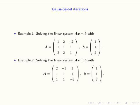
I Example 1: Solving the linear system Ax = b with
A =
1 2 −2
1 1 1
2 2 1
, b =
1
1
2
.
I Example 2: Solving the linear system Ax = b with
A =
2 −1 1
1 1 1
1 1 −2
, b =
1
1
2
.
Gauss-Seidel iterations
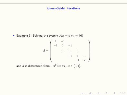
I Example 3: Solving the system Ax = b (n = 30)
A =
2 −1
−1 2 −1
. . .. . .
. . .
−1 2 −1
−1 2
and b is discretized from −π2 sinπx, x ∈ [0, 1].
Gauss-Seidel iterations
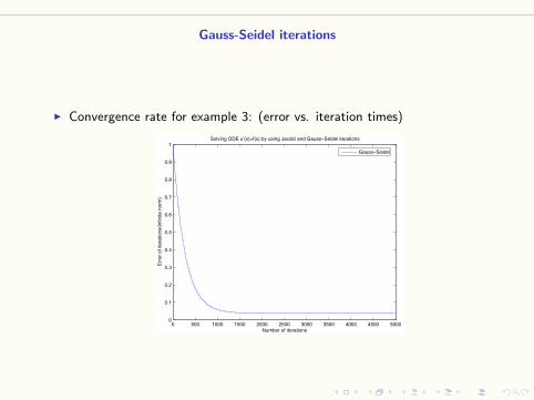
I Convergence rate for example 3: (error vs. iteration times)
0 500 1000 1500 2000 2500 3000 3500 4000 4500 50000
0.1
0.2
0.3
0.4
0.5
0.6
0.7
0.8
0.9
1
Number of iterations
Err
or o
f ite
ratio
ns(in
finite
nor
m)
Solving ODE u’(x)=f(x) by using Jacobi and Gauss−Seidel iterations
Gauss−Seidel
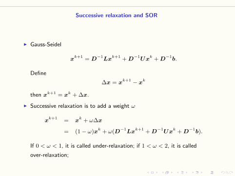
Successive relaxation and SOR
I Gauss-Seidel
xk+1 = D−1Lxk+1 + D−1Uxk + D−1b.
Define
∆x = xk+1 − xk
then xk+1 = xk + ∆x.
I Successive relaxation is to add a weight ω
xk+1 = xk + ω∆x
= (1− ω)xk + ω(D−1Lxk+1 + D−1Uxk + D−1b).
If 0 < ω < 1, it is called under-relaxation; if 1 < ω < 2, it is called
over-relaxation;
Convergence theorem
Theorem (Necessary condition)
The necessary condition for the convergence of SR method is
0 < ω < 2
Theorem (SPD matrix)
If A is symmetric positive definite, then
0 < ω < 2
is the sufficient condition for convergence.
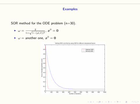
Examples
SOR method for the ODE problem (n=30).
I ω = 2
1+√
1−(ρ(J))2, x0 = 0
I ω = another one, x0 = 0
0 100 200 300 400 500 600 700 800 900 10000
0.1
0.2
0.3
0.4
0.5
0.6
0.7
0.8
0.9
1
Number of iterations
Err
or o
f ite
ratio
ns(in
finite
nor
m)
Solving ODE u’(x)=f(x) by using SOR for different relaxational factors
Optimal SORNormal SOR

Outline
Puzzle?
I Arbitrary decomposition (F is invertible)
A = F −G
then the linear system is transformed into
x = F−1Gx + F−1b.
and construct the iteration
xk+1 = F−1Gxk + F−1b.
How about the result?
I A simpler case (1D case) ax = b, a = f − g then construct
xk+1 = f−1gxk + f−1b.
How about the convergence?
Analysis for simple case
I Linear system ax = b
Exact solution x∗ = f−1gx∗ + f−1b
Iteration xk+1 = f−1gxk + f−1b.
I Subtract two expressions and define error ek = xk − x∗ thus
ek+1 = f−1gek
Then |ek| = |f−1g|k|e0|. In order |ek| → 0, we must have
|f−1g| < 1
That’s the convergence condition for 1D case.
A fundamental theorem
I Spectral radius
The spectral radius of a matrix A is defined as
ρ(A) = maxλ|λ(A)|
Theorem (Spectral radius and iterative convergence)
If A ∈ Rn, then
limk→0
Ak = 0 ⇐⇒ ρ(A) < 1
Analysis for general case
I Linear system Ax = b
Exact solution x∗ = Bx∗ + g
Iteration xk+1 = Bxk + g
I Subtract two expressions and define error ek = xk − x∗ thus
ek+1 = Bek
By induction we have
ek = Bke0.
Thus we have
ek → 0 ⇐⇒ Bk → 0 ⇐⇒ ρ(B) < 1
That’s the convergence criterion for general iterations.
Examples
I Analysis for example 1.
Spectral radius for Jacobi:
Spectral radius for Gauss-Seidel:
I Analysis for example 2.
Spectral radius for Jacobi:
Spectral radius for Gauss-Seidel:
Rate of convergence
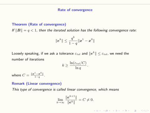
Theorem (Rate of convergence)
If ‖B‖ = q < 1, then the iterated solution has the following convergence rate:
‖ek‖ ≤ qk
1− q‖x1 − x0‖
Loosely speaking, if we ask a tolerance εtol and ‖ek‖ ≤ εtol, we need the
number of iterations
k ≥ ln(εtol/C)
ln q.
where C = ‖x1−x0‖1−q
.
Remark (Linear convergence)
This type of convergence is called linear convergence, which means
limk→∞
‖ek+1‖‖ek‖ = C 6= 0.
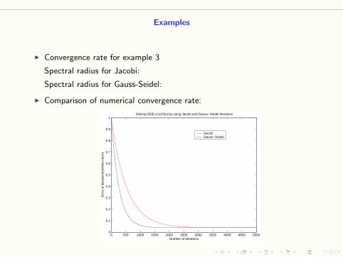
Examples
I Convergence rate for example 3
Spectral radius for Jacobi:
Spectral radius for Gauss-Seidel:
I Comparison of numerical convergence rate:
0 500 1000 1500 2000 2500 3000 3500 4000 4500 50000
0.1
0.2
0.3
0.4
0.5
0.6
0.7
0.8
0.9
1
Number of iterations
Err
or o
f ite
ratio
ns(in
finite
nor
m)
Solving ODE u’(x)=f(x) by using Jacobi and Gauss−Seidel iterations
JacobiGauss−Seidel
Diagonally dominant matrix and its properties
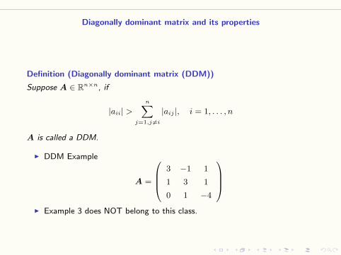
Definition (Diagonally dominant matrix (DDM))
Suppose A ∈ Rn×n, if
|aii| >n∑
j=1,j 6=i
|aij |, i = 1, . . . , n
A is called a DDM.
I DDM Example
A =
3 −1 1
1 3 1
0 1 −4
I Example 3 does NOT belong to this class.
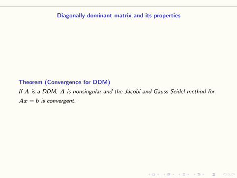
Diagonally dominant matrix and its properties
Theorem (Convergence for DDM)
If A is a DDM, A is nonsingular and the Jacobi and Gauss-Seidel method for
Ax = b is convergent.

Outline
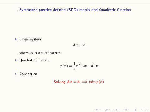
Symmetric positive definite (SPD) matrix and Quadratic function
I Linear system
Ax = b
where A is a SPD matrix.
I Quadratic function
ϕ(x) =1
2xT Ax− bT x
I Connection
Solving Ax = b ⇐⇒ minϕ(x)
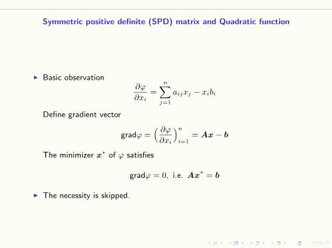
Symmetric positive definite (SPD) matrix and Quadratic function
I Basic observation∂ϕ
∂xi=
n∑j=1
aijxj − xibi
Define gradient vector
gradϕ =( ∂ϕ∂xi
)n
i=1= Ax− b
The minimizer x∗ of ϕ satisfies
gradϕ = 0, i.e. Ax∗ = b
I The necessity is skipped.
Symmetric positive definite (SPD) matrix and Quadratic function
The connection between linear system and quadratic function minimization
tells us if we have an algorithm to deal with quadratic function minimization
we have an algorithm for solving the linear system.
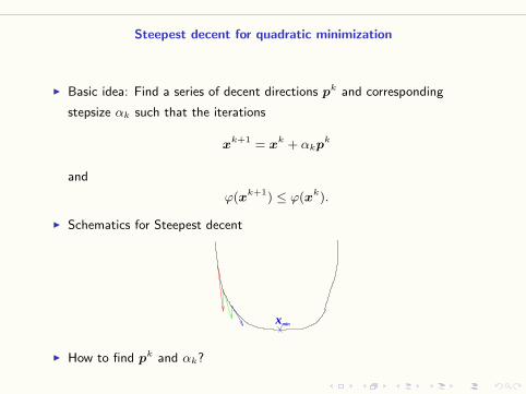
Steepest decent for quadratic minimization
I Basic idea: Find a series of decent directions pk and corresponding
stepsize αk such that the iterations
xk+1 = xk + αkpk
and
ϕ(xk+1) ≤ ϕ(xk).
I Schematics for Steepest decent
xmin
I How to find pk and αk?
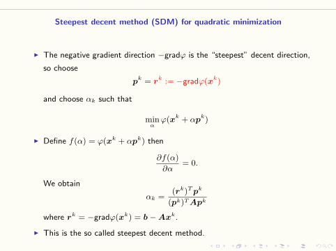
Steepest decent method (SDM) for quadratic minimization
I The negative gradient direction −gradϕ is the “steepest” decent direction,
so choose
pk = rk := −gradϕ(xk)
and choose αk such that
minαϕ(xk + αpk)
I Define f(α) = ϕ(xk + αpk) then
∂f(α)
∂α= 0.
We obtain
αk =(rk)T pk
(pk)T Apk
where rk = −gradϕ(xk) = b−Axk.
I This is the so called steepest decent method.

Example
I Example 1:
A =
4 1 1 0
1 4 1 1
1 1 4 1
0 1 1 4
b =
6
7
7
6
I The ODE example (n=30):
Convergence rate.
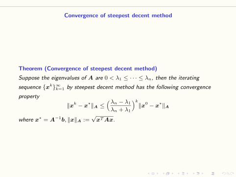
Convergence of steepest decent method
Theorem (Convergence of steepest decent method)
Suppose the eigenvalues of A are 0 < λ1 ≤ · · · ≤ λn, then the iterating
sequence {xk}∞k=1 by steepest decent method has the following convergence
property
‖xk − x∗‖A ≤(λn − λ1
λn + λ1
)k
‖x0 − x∗‖A
where x∗ = A−1b, ‖x‖A :=√
xT Ax.
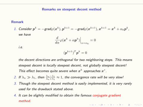
Remarks on steepest decent method
Remark
1. Consider pk = −gradϕ(xk),pk+1 = −gradϕ(xk+1),xk+1 = xk + αkpk,
we haved
dαϕ(xk + αpk)
∣∣∣α=αk
= 0
i.e.
(pk+1)T pk = 0
the decent directions are orthogonal for two neighboring steps. This means
steepest decent is locally steepest decent, not globally steepest decent!
This effect becomes quite severe when xk approaches x∗.
2. If λn � λ1, then λn−λ1λn+λ1
≈ 1, the convergence rate will be very slow!
3. Though the steepest decent method is easily implemented, it is very rarely
used for the drawback stated above.
4. It can be slightly modified to obtain the famous conjugate gradient
method.
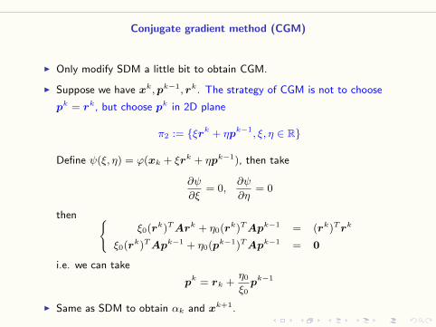
Conjugate gradient method (CGM)
I Only modify SDM a little bit to obtain CGM.
I Suppose we have xk,pk−1, rk. The strategy of CGM is not to choose
pk = rk, but choose pk in 2D plane
π2 := {ξrk + ηpk−1, ξ, η ∈ R}
Define ψ(ξ, η) = ϕ(xk + ξrk + ηpk−1), then take
∂ψ
∂ξ= 0,
∂ψ
∂η= 0
then {ξ0(r
k)T Ark + η0(rk)T Apk−1 = (rk)T rk
ξ0(rk)T Apk−1 + η0(p
k−1)T Apk−1 = 0
i.e. we can take
pk = rk +η0ξ0
pk−1
I Same as SDM to obtain αk and xk+1.
Conjugate gradient method (CGM)
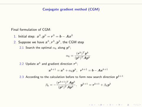
Final formulation of CGM:
1. Initial step: x0,p0 = r0 = b−Ax0
2. Suppose we have xk, rk,pk, the CGM step
2.1 Search the optimal αk along pk;
αk =(rk)T pk
(pk)T Apk
2.2 Update xk and gradient direction rk;
xk+1 = xk + αkpk, rk+1 = b − Axk+1
2.3 According to the calculation before to form new search direction pk+1
βk = −(rk+1)T Apk
(pk)T Apk, pk+1 = rk+1 + βkpk
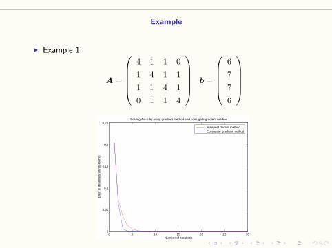
Example
I Example 1:
A =
4 1 1 0
1 4 1 1
1 1 4 1
0 1 1 4
b =
6
7
7
6
0 5 10 15 20 25 300
0.05
0.1
0.15
0.2
0.25
Number of iterations
Err
or o
f ite
ratio
ns(in
finite
nor
m)
Solving Ax=b by using gradient method and conjugate gradient method
Steepest decent methodConjugate gradient method
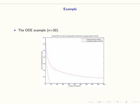
Example
I The ODE example (n=30):
0 50 100 150 200 250 300 350 400 450 5000
0.1
0.2
0.3
0.4
0.5
0.6
0.7
Number of iterations
Err
or o
f ite
ratio
ns(in
finite
nor
m)
Solving ODE u’(x)=f(x) by using gradient method and conjugate gradient method
Steepest decent methodConjugate gradient method
Properties of CGM
Theorem
The vectors generated by CGM have the properties
1. (ri)T rj = 0, i 6= j, 0 ≤ i < j ≤ k;
2. (pi)T Apj = 0, i 6= j, 0 ≤ i < j ≤ k;
I The property (pi)T Apj = 0 makes {pj}j=1,2,... are called conjugate
directions of A. From property 1, we have
Theoretically, CGM will find the minimum (or solution) within n steps.
This is not the case in real computations. CGM is applied as an iteration.
I Virtue of CGM: Suitable for sparse matrix A, without adjustable
parameters as SOR.
Convergence of CGM
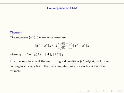
Theorem
The sequence {xk} has the error estimate
‖xk − x∗‖A ≤ 2(√κ2 − 1√κ2 + 1
)‖x0 − x∗‖A
where κ2 := Cond2(A) = ‖A‖2‖A−1‖2.
This theorem tells us if the matrix in good condition (Cond2(A) ≈ 1), the
convergence is very fast. The real computations are even faster than the
estimate.
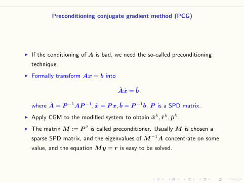
Preconditioning conjugate gradient method (PCG)
I If the conditioning of A is bad, we need the so-called preconditioning
technique.
I Formally transform Ax = b into
Ax = b
where A = P−1AP−1, x = Px, b = P−1b, P is a SPD matrix.
I Apply CGM to the modified system to obtain xk, rk, pk.
I The matrix M := P 2 is called preconditioner. Usually M is chosen a
sparse SPD matrix, and the eigenvalues of M−1A concentrate on some
value, and the equation My = r is easy to be solved.
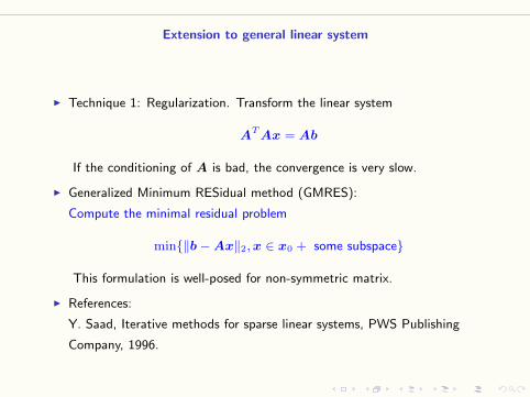
Extension to general linear system
I Technique 1: Regularization. Transform the linear system
AT Ax = Ab
If the conditioning of A is bad, the convergence is very slow.
I Generalized Minimum RESidual method (GMRES):
Compute the minimal residual problem
min{‖b−Ax‖2,x ∈ x0 + some subspace}
This formulation is well-posed for non-symmetric matrix.
I References:
Y. Saad, Iterative methods for sparse linear systems, PWS Publishing
Company, 1996.
Homework assignment 3
1. Using Gauss-Seidel and conjugate gradient method to solve the second order
ODEs(n=30, 50, 100). Plot the figure for the convergence rate.


![Solving Linear Systems: Iterative Methods and Sparse · PDF fileSolving Linear Systems: Iterative Methods and Sparse Systems ... [non-singular] matrix O(n3) LU decomposition Works](https://img.pdfslide.net/doc/110x75/5a7957ed7f8b9ac53b8d88c9/solving-linear-systems-iterative-methods-and-sparse-linear-systems-iterative.jpg)