Embed Size (px)
Citation preview

8/3/2019 Lecture-36 Shortest Path Algorithms
http://slidepdf.com/reader/full/lecture-36-shortest-path-algorithms 1/23
Shortest Path
Algorithms
8/3/2019 Lecture-36 Shortest Path Algorithms
http://slidepdf.com/reader/full/lecture-36-shortest-path-algorithms 2/23
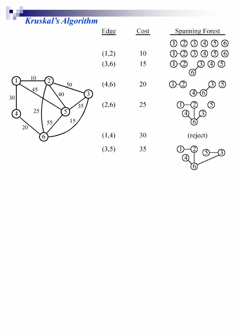
Kruskal¶s Algorithm
We construct a set of edges A satisfying thefollowing invariant:
A is a subset of someMST
We start with A empty
On each iteration, we add
a suitable edge to A In the case of Kruskal¶s
algorithm, candidateedges are considered inorder by increasing
weight
MST-Kruskal (G,w)
A <- For each vertex v V[G]
M ake-Set(v)
sort the edges(E) in
increasing order by
weight w
for each edge (u,v) Eif FindSet(u) { FindSet(v)
A = A U {(u,v)}
UNION(u,v)
8/3/2019 Lecture-36 Shortest Path Algorithms
http://slidepdf.com/reader/full/lecture-36-shortest-path-algorithms 3/23
Kruskal¶s Algorithm
8/3/2019 Lecture-36 Shortest Path Algorithms
http://slidepdf.com/reader/full/lecture-36-shortest-path-algorithms 4/23
Application: The Minimal-
Connector Problem
Given a connected graph in which each edgehas a weight , find a spanning tree with
minimum total cost. Kruskal's Al gor ithm: Build tree by repeatedly
adding min-weight edge that doesn't form a cycle
P r im's Al gor ithm: Build tree by adding v er tices,adjacent to tree so far, for which new edges havemin weight and don't form cycle
8/3/2019 Lecture-36 Shortest Path Algorithms
http://slidepdf.com/reader/full/lecture-36-shortest-path-algorithms 5/23
Properties of Kruskal¶s and Prim¶s
Algorithms
Both are greedy : They take the best
immediate choice without considering
future ramifications
Greedy algorithms don¶t always work best, but
these do.
Prim always maintains a connected graph,while Kruskal may not.
8/3/2019 Lecture-36 Shortest Path Algorithms
http://slidepdf.com/reader/full/lecture-36-shortest-path-algorithms 6/23
Measuring Efficiency of Graph
Algorithms
Efficiency = Time complexity = (roughly)
how many steps are needed as a function
of N (number of vertices) and E (number
of edges)
For any graph, 0 e E e N(N-1)/2 = O(N2)
For any connected graph, N-1 e E e N(N-1)/2 , O(N) e E e O(N2)
8/3/2019 Lecture-36 Shortest Path Algorithms
http://slidepdf.com/reader/full/lecture-36-shortest-path-algorithms 7/23
Running time of
Kruskal Algorithm
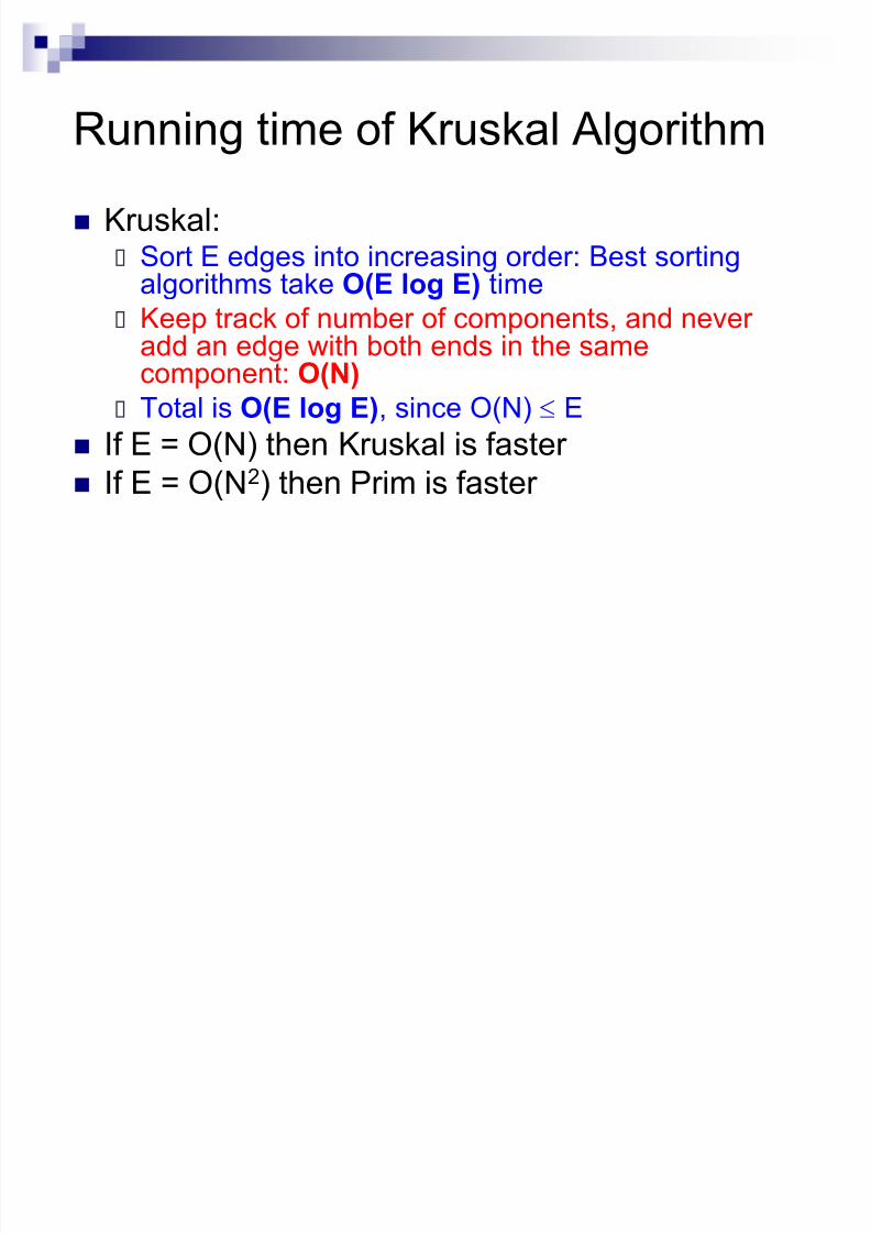
Kruskal: Sort E edges into increasing order: Best sorting
algorithms take O(E log E) time
Keep track of number of components, and never add an edge with both ends in the samecomponent: O(N)
Total is O(E log E), since O(N) e E
If E = O(N) thenK
ruskal is faster If E = O(N2) then Prim is faster

8/3/2019 Lecture-36 Shortest Path Algorithms
http://slidepdf.com/reader/full/lecture-36-shortest-path-algorithms 8/23
Shortest Path Problem in Graphs
8/3/2019 Lecture-36 Shortest Path Algorithms
http://slidepdf.com/reader/full/lecture-36-shortest-path-algorithms 9/23
Problem A motorist wishes to find the shortest possible route
from Islamabad to Lahore.
Route map is given where distance between each pair of adjacent intersections is marked.
One possible way is to enumerate all the routes from
Islamabad to Lahore, add up the distance on each
route and select the shortest.
There are hundreds and thousands of possibilities,
most of them are simply not worth considering.
8/3/2019 Lecture-36 Shortest Path Algorithms
http://slidepdf.com/reader/full/lecture-36-shortest-path-algorithms 10/23
Contd« A route from Islamabad to Peshawar to Lahore is
obviously a poor choice, as Peshawar is hundreds of
miles out of the way.
In this presentation, we show how to solve such
problems efficiently.
8/3/2019 Lecture-36 Shortest Path Algorithms
http://slidepdf.com/reader/full/lecture-36-shortest-path-algorithms 11/23
Shortest path problemWe are given a weighted, graph G=(V,E),
with weight function w:E->R mapping
edges to real-valued weights.
The weight of path p=<v0,v1,«vk> is the
sum of the weights of its constituentedges.
8/3/2019 Lecture-36 Shortest Path Algorithms
http://slidepdf.com/reader/full/lecture-36-shortest-path-algorithms 12/23
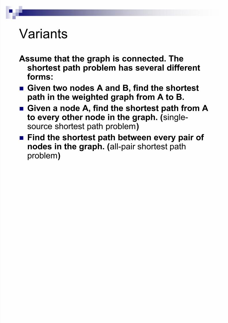
VariantsAssume that the graph is connected. The
shortest path problem has several different
forms: Given two nodes A and B, find the shortest
path in the weighted graph from A to B. Given a node A, find the shortest path from A
to every other node in the graph. (single-source shortest path problem) Find the shortest path between every pair of
nodes in the graph. (all-pair shortest path
problem)
8/3/2019 Lecture-36 Shortest Path Algorithms
http://slidepdf.com/reader/full/lecture-36-shortest-path-algorithms 13/23
Single-Source Shortest Path Problem: given a weighted graph G, find
the minimum-weight path from a given
source vertex s to another vertex v
³Shortest-path´ = minimum weight
Weight of path is sum of edges
8/3/2019 Lecture-36 Shortest Path Algorithms
http://slidepdf.com/reader/full/lecture-36-shortest-path-algorithms 14/23
Dijkstra¶s Algorithm
Similar to breadth-first search
Grow a tree gradually, advancing from vertices
taken from a queue
Also similar to Prim¶s algorithm for MST
Use a priority queue keyed on d[v]
8/3/2019 Lecture-36 Shortest Path Algorithms
http://slidepdf.com/reader/full/lecture-36-shortest-path-algorithms 15/23
Dijkstra¶s Algorithm
The idea is to visit the nodes in order of their closeness to
A; visit A first, then visit the closest node to A, then the next
closest node to A, and so on.
The closest node to A, say X , must be adjacent to A and the
next closest node, say Y , must be either adjacent to A or X .
The third closest node to A must be either adjacent to A or X
or Y , and so on. (Otherwise, this node is closer to A than the
third closest node.)
8/3/2019 Lecture-36 Shortest Path Algorithms
http://slidepdf.com/reader/full/lecture-36-shortest-path-algorithms 16/23
The next node to be visited must be adjacent to some visited
node. We call the set of unvisited nodes that are adjacent to an
already visited node the fringe.
The algorithm then selects the node from the fringe closest toA, say B, then visits B and updates the fringe to include the
nodes that are adjacent to B. This step is repeated until all the
nodes of the graph have been visited and the fringe is empty.
Dijkstra¶s Algorithm
8/3/2019 Lecture-36 Shortest Path Algorithms
http://slidepdf.com/reader/full/lecture-36-shortest-path-algorithms 17/23
Dijkstra¶s Algorithm
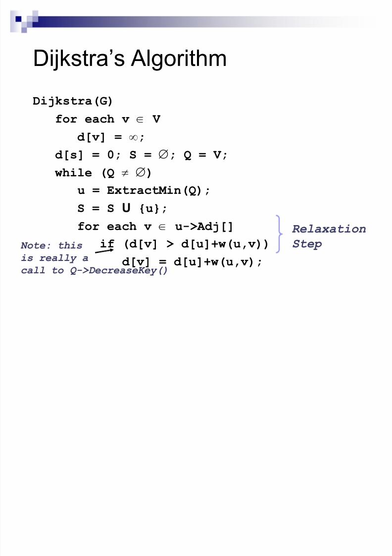
Dijkstra(G)
for each v V
d [v] = g;d [s] = 0; S = ; Q = V ;
while (Q { )
u = Extract M in(Q);
S = S U {u};
for each v u->Adj[]
if (d [v] > d [u]+ w(u,v))
d [v] = d [u]+ w(u,v);
Relaxation
Step Note: this
is really a
call to Q->DecreaseKey()
8/3/2019 Lecture-36 Shortest Path Algorithms
http://slidepdf.com/reader/full/lecture-36-shortest-path-algorithms 18/23
Dijkstra¶s Algorithm
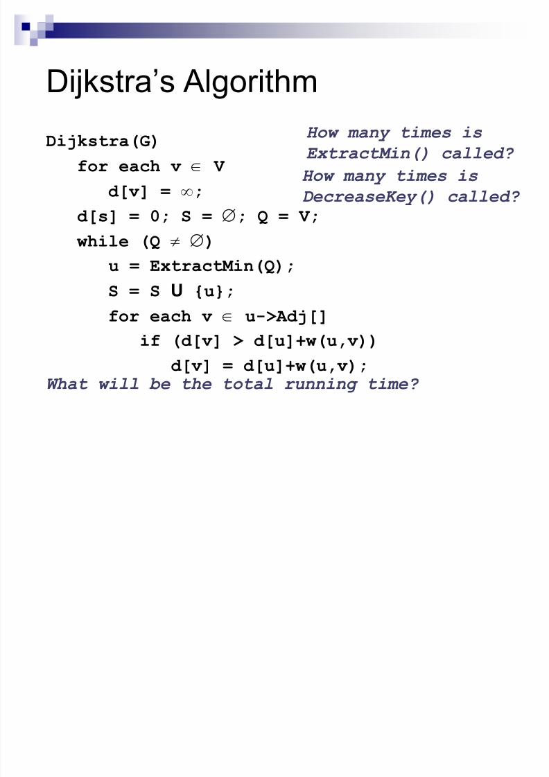
Dijkstra(G)
for each v V
d [v] = g;d [s] = 0; S = ; Q = V ;
while (Q { )
u = Extract M in(Q);
S = S U {u};
for each v u->Adj[]
if (d [v] > d [u]+ w(u,v))
d [v] = d [u]+ w(u,v);
H ow many times is
ExtractMin() called?
H ow many times is
DecreaseKey() called?
What will be the total running time?
8/3/2019 Lecture-36 Shortest Path Algorithms
http://slidepdf.com/reader/full/lecture-36-shortest-path-algorithms 19/23
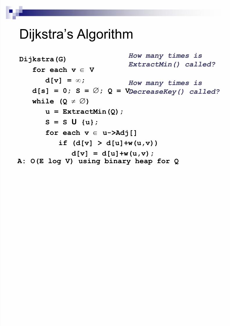
Dijkstra¶s Algorithm
Dijkstra(G)
for each v V
d [v] = g;d [s] = 0; S = ; Q = V ;
while (Q { )
u = Extract M in(Q);
S = S U {u};
for each v u->Adj[]
if (d [v] > d [u]+ w(u,v))
d [v] = d [u]+ w(u,v);
H ow many times is
ExtractMin() called?
H ow many times is
DecreaseKey() called?
A: O(E log V ) using binary heap for Q
8/3/2019 Lecture-36 Shortest Path Algorithms
http://slidepdf.com/reader/full/lecture-36-shortest-path-algorithms 20/23
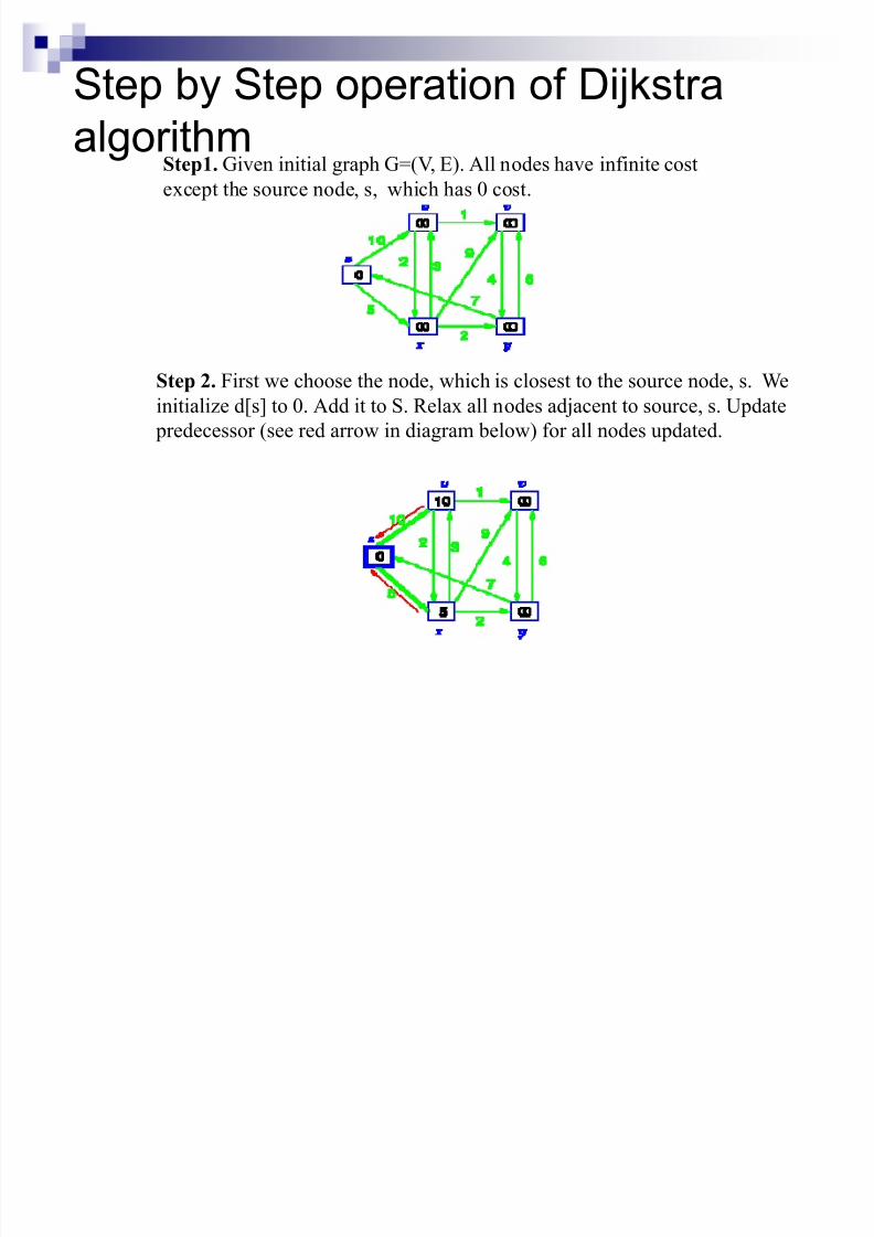
Step by Step operation of Dijkstra
algorithmStep1. Given initial graph G=(V, E). All nodes have infinite cost
except the source node, s, which has 0 cost.
Step 2. First we choose the node, which is closest to the source node, s. We
initialize d[s] to 0. Add it to S. Relax all nodes adjacent to source, s. Update
predecessor (see red arrow in diagram below) for all nodes updated.
8/3/2019 Lecture-36 Shortest Path Algorithms
http://slidepdf.com/reader/full/lecture-36-shortest-path-algorithms 21/23
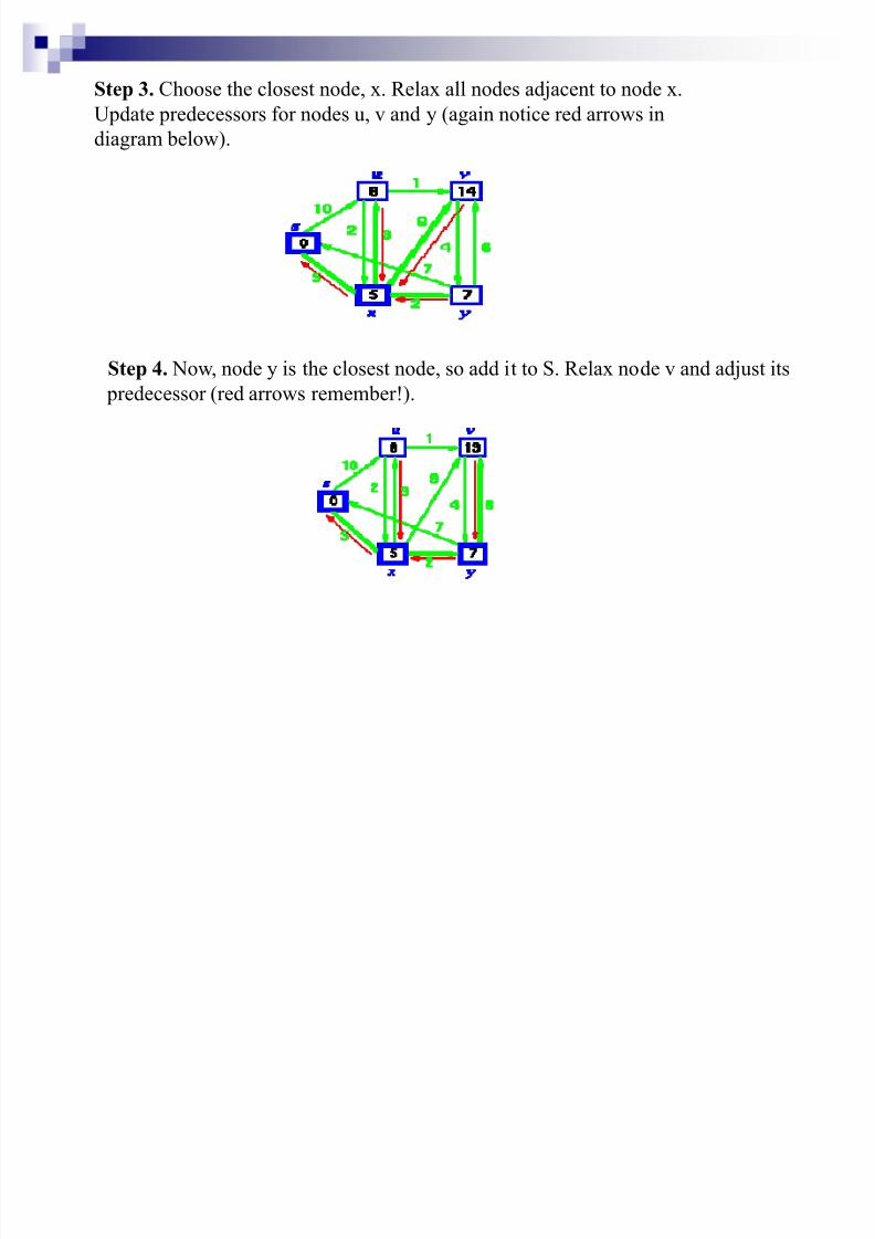
Step 3. Choose the closest node, x. Relax all nodes adjacent to node x.
Update predecessors for nodes u, v and y (again notice red arrows in
diagram below).
Step 4. Now, node y is the closest node, so add it to S. Relax node v and adjust its
predecessor (red arrows remember!).
8/3/2019 Lecture-36 Shortest Path Algorithms
http://slidepdf.com/reader/full/lecture-36-shortest-path-algorithms 22/23
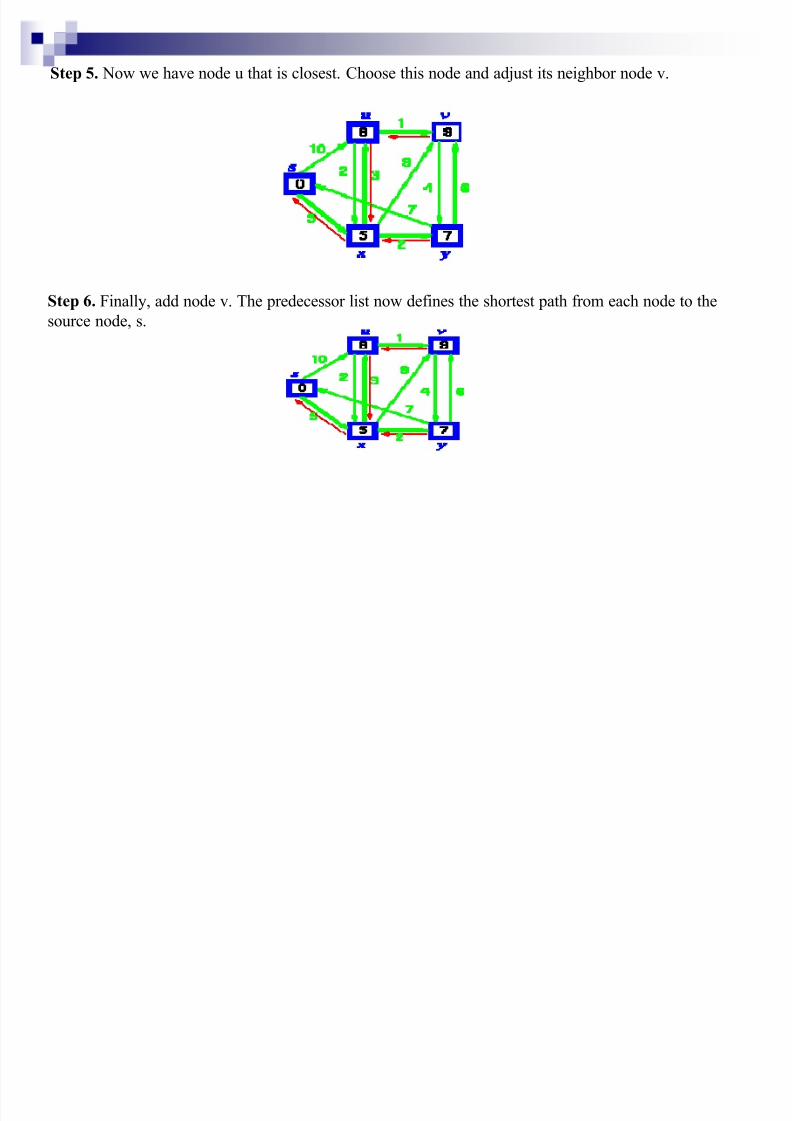
Step 5. Now we have node u that is closest. Choose this node and adjust its neighbor node v.
Step 6. Finally, add node v. The predecessor list now defines the shortest path from each node to the
source node, s.
8/3/2019 Lecture-36 Shortest Path Algorithms
http://slidepdf.com/reader/full/lecture-36-shortest-path-algorithms 23/23
Analysis of D
ijkstra AlgorithmQ as a linear array
EXTR ACT_MIN takes O(V) time and there are |V| such operations.Therefore, a total time for EXTR ACT_MIN in while-loop is O(V2).Since the total number of edges in all the adjacency list is |E|.
Therefore for-loop iterates |E| times with each iteration taking O(1)time. Hence, the running time of the algorithm with arrayimplementation is O(V2 + E) = O(V2).
Q as a binary heap ( If G is sparse)In this case, EXTR ACT_MIN operations takes O(log V) time andthere are |V| such operations. The binary heap can be build in O(V)time. Operation DECREASE (in the RELAX) takes O(log V) time andthere are at most such operations.Hence, the running time of the algorithm with binary heap providedgiven graph is sparse is O((V + E) log V). Note that this timebecomes O(E logV) if all vertices in the graph is reachable from thesource vertices.


![Graph Algorithms Shortest path problems [Adapted from K.Wayne]](https://img.pdfslide.net/doc/110x75/56649d4e5503460f94a2e1c6/graph-algorithms-shortest-path-problems-adapted-from-kwayne.jpg)