Embed Size (px)
Citation preview
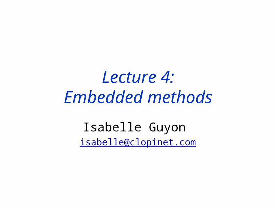
Filters,Wrappers, andEmbedded methods
All features FilterFeature subset Predictor
All features
Wrapper
Multiple Feature subsets
Predictor
All featuresEmbedded
method
Feature subset
Predictor
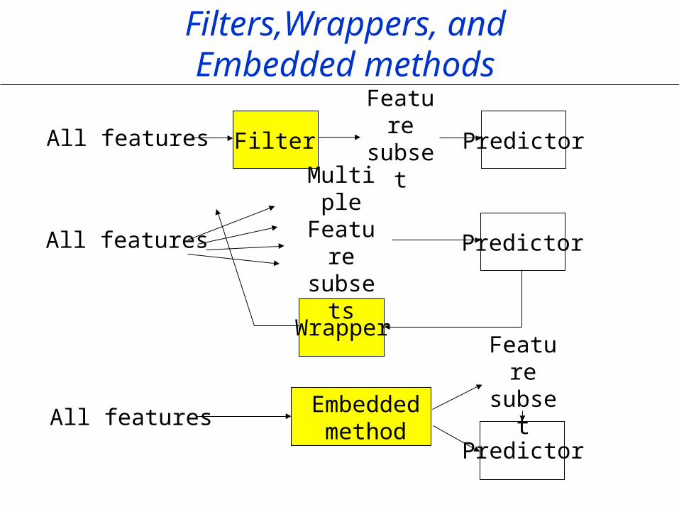
Filters
• Criterion: Measure feature/feature subset “relevance”
• Search: Usually order features (individual feature ranking or nested subsets of features)
• Assessment: Use statistical tests
• Are (relatively) robust against overfitting• May fail to select the most “useful” features
Methods:
Results:
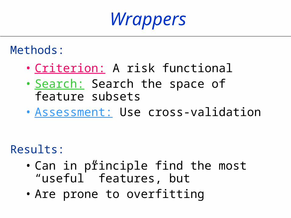
Wrappers
• Criterion: A risk functional• Search: Search the space of feature
subsets• Assessment: Use cross-validation
• Can in principle find the most “useful” features, but
• Are prone to overfitting
Methods:
Results:
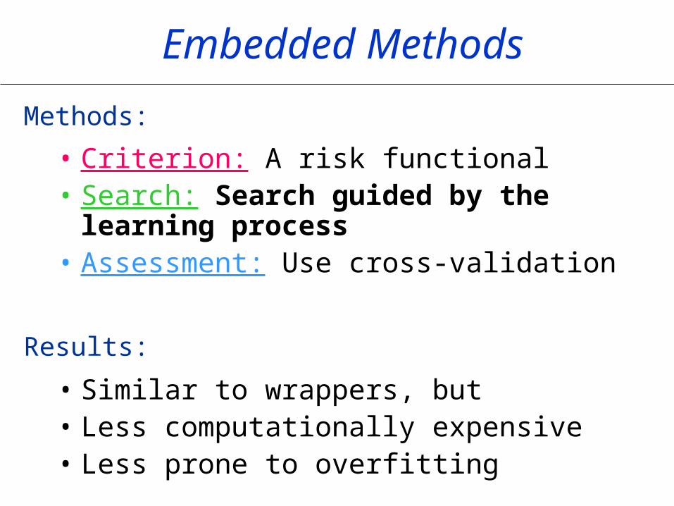
Embedded Methods
• Criterion: A risk functional• Search: Search guided by the
learning process• Assessment: Use cross-validation
• Similar to wrappers, but• Less computationally expensive• Less prone to overfitting
Methods:
Results:
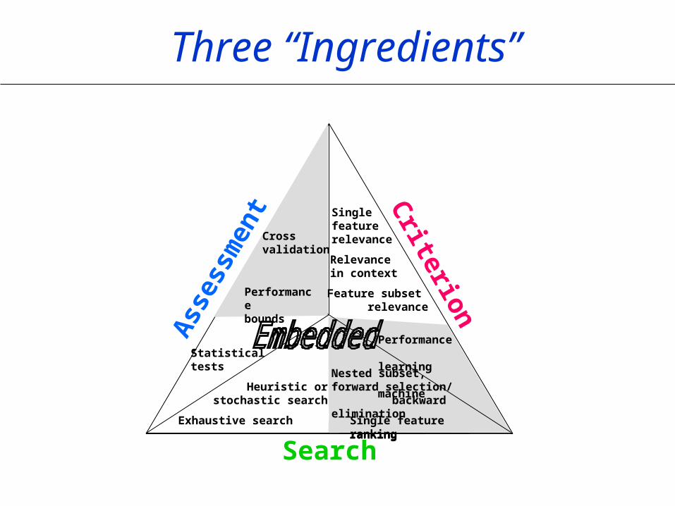
Statistical tests
Single feature ranking
Cross validation
Performance bounds
Nested subset,forward selection/ backward elimination
Heuristic orstochastic search
Exhaustive search
Single featurerelevance
Relevancein context
Feature subset relevance
Performance learning machine
Search
Criterion
Ass
essm
ent
Statistical tests
Single feature ranking
Cross validation
Performance bounds
Nested subset,forward selection/ backward elimination
Heuristic orstochastic search
Exhaustive search
Single featurerelevance
Relevancein context
Feature subset relevance
Performance learning machine
Three “Ingredients”
Statistical tests
Single feature ranking
Cross validation
Performance bounds
Nested subset,forward selection/ backward elimination
Heuristic orstochastic search
Exhaustive search
Single featurerelevance
Relevancein context
Feature subset relevance
Performance learning machine
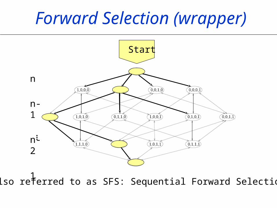
Forward Selection (wrapper)
n
n-1
n-2
1
…
Start
Also referred to as SFS: Sequential Forward Selection
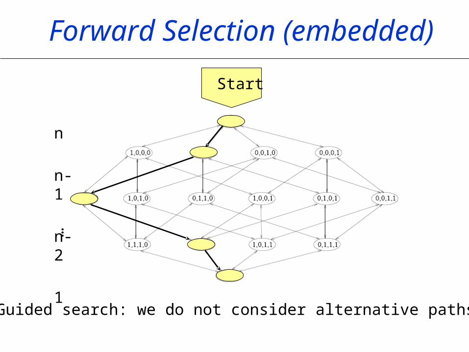
Guided search: we do not consider alternative paths.
Forward Selection (embedded)
…
Start
n
n-1
n-2
1
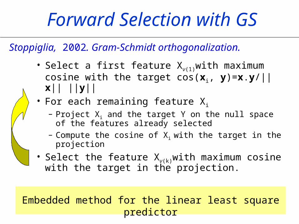
Forward Selection with GS
• Select a first feature Xν(1)with maximum cosine with the target cos(xi, y)=x.y/||x|| ||y||
• For each remaining feature Xi
– Project Xi and the target Y on the null space of the features already selected
– Compute the cosine of Xi with the target in the projection
• Select the feature Xν(k)with maximum cosine with the target in the projection.
Embedded method for the linear least square predictor
Stoppiglia, 2002. Gram-Schmidt orthogonalization.
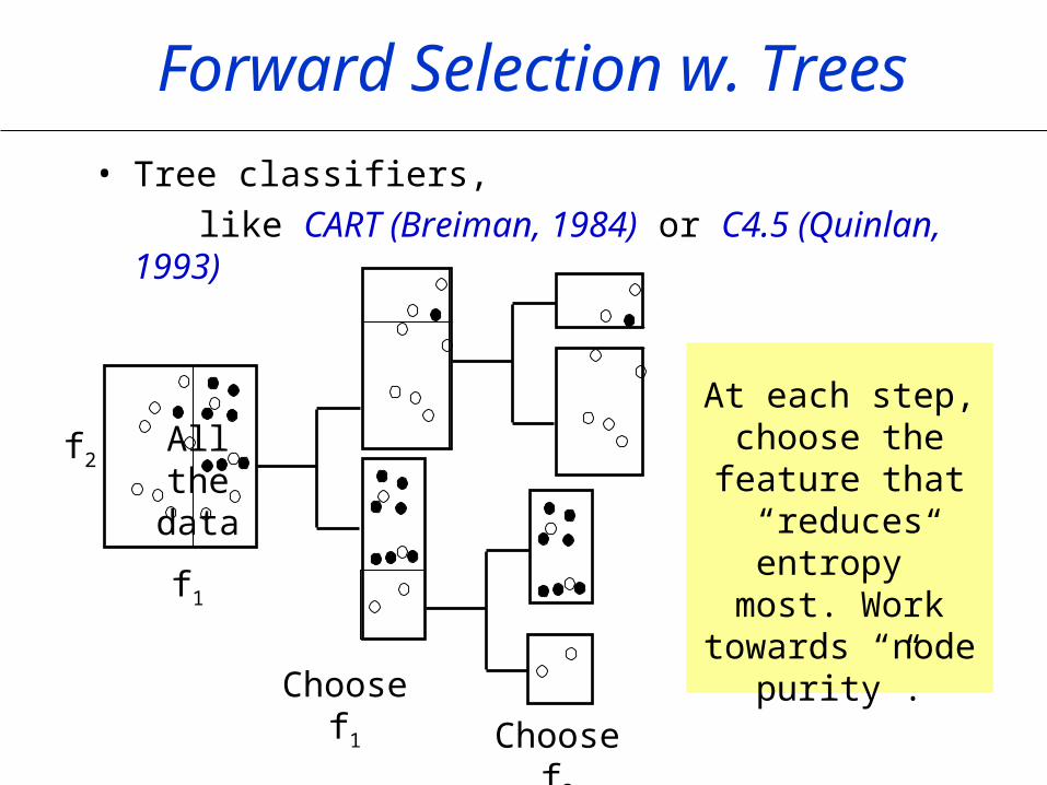
Forward Selection w. Trees
• Tree classifiers,
like CART (Breiman, 1984) or C4.5 (Quinlan, 1993)
At each step, choose the feature that
“reduces entropy” most. Work
towards “node purity”.
All the data
f1
f2
Choose f1
Choose f2
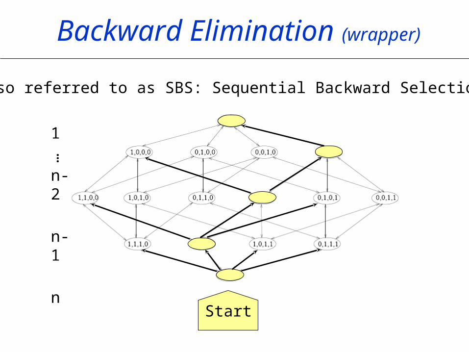
Backward Elimination (wrapper)
1
n-2
n-1
n
…
Start
Also referred to as SBS: Sequential Backward Selection
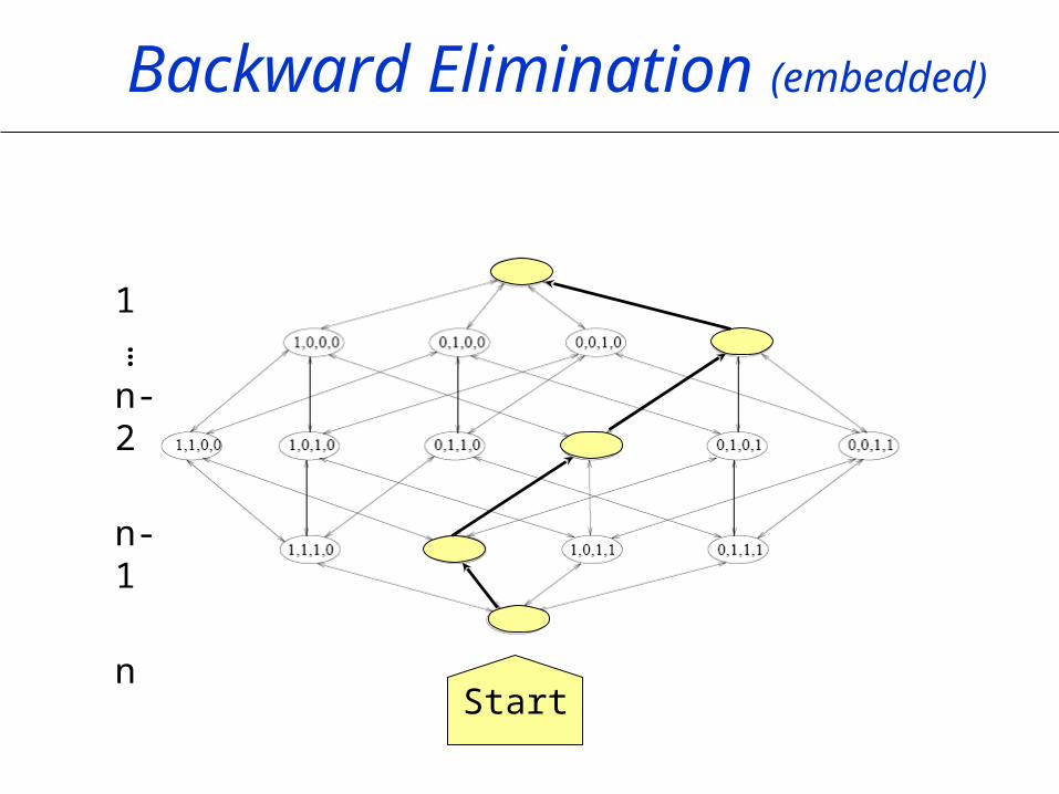
Backward Elimination (embedded)
…
Start
1
n-2
n-1
n
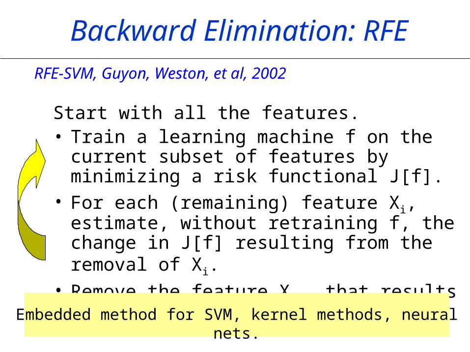
Backward Elimination: RFE
Start with all the features.• Train a learning machine f on the current subset
of features by minimizing a risk functional J[f].• For each (remaining) feature Xi, estimate,
without retraining f, the change in J[f] resulting from the removal of Xi.
• Remove the feature Xν(k) that results in improving or least degrading J.
Embedded method for SVM, kernel methods, neural nets.
RFE-SVM, Guyon, Weston, et al, 2002
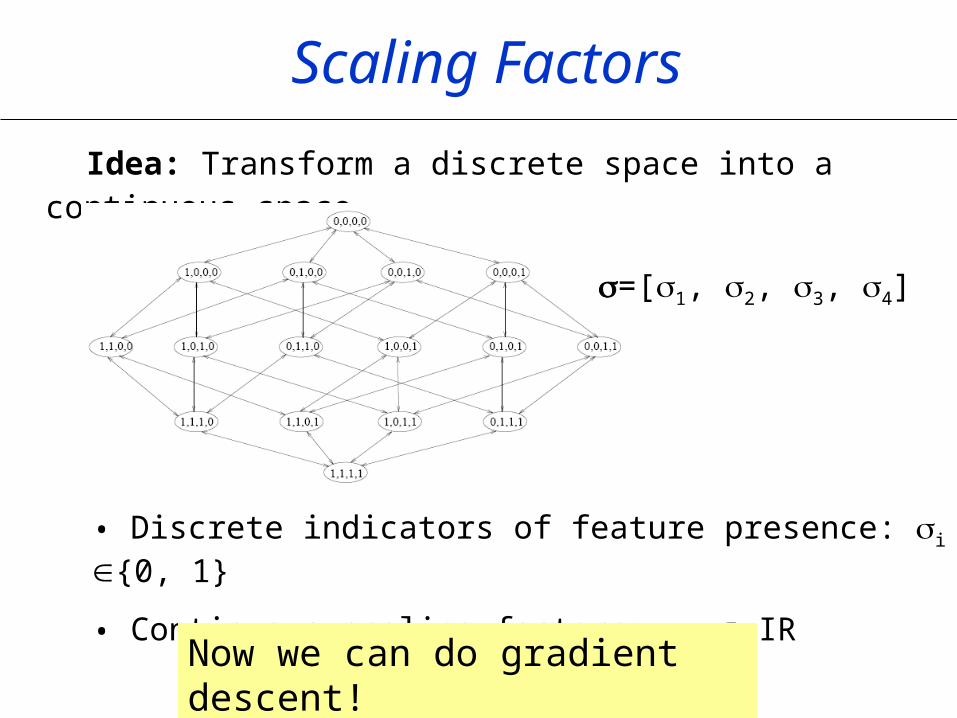
Scaling Factors
Idea: Transform a discrete space into a continuous space.
• Discrete indicators of feature presence: i {0, 1}
• Continuous scaling factors: i IR
=[1, 2, 3, 4]
Now we can do gradient descent!
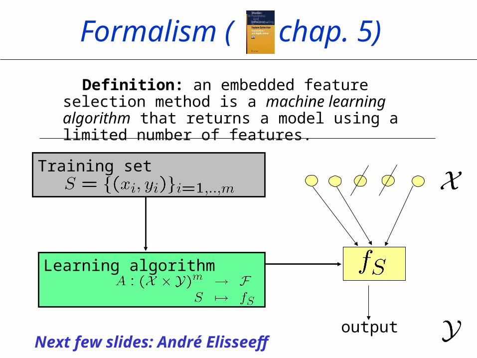
Definition: an embedded feature selection method is a machine learning algorithm that returns a model using a limited number of features.
Training set
Learning algorithm
output
Formalism ( chap. 5)
Next few slides: André Elisseeff
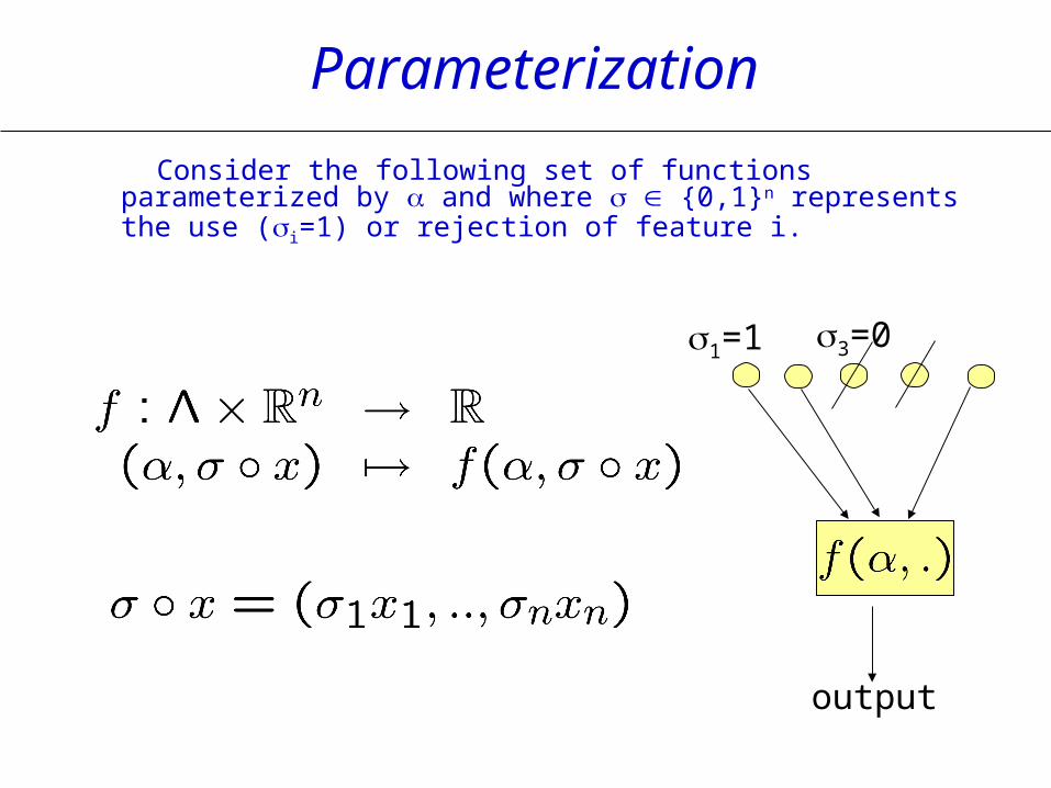
Consider the following set of functions parameterized by and where {0,1}n represents the use (i=1) or rejection of feature i.
output
1=1 3=0
Parameterization
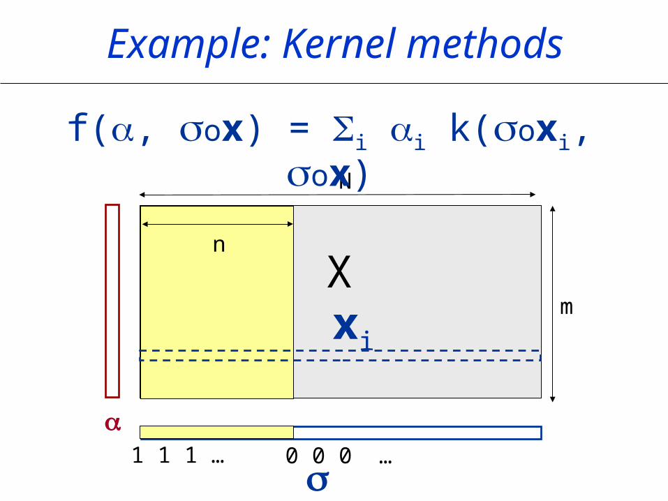
Example: Kernel methods
X
N
m
f(, ox) = i i k(oxi, ox)
xi
1 1 1 … 0 0 0 …
n
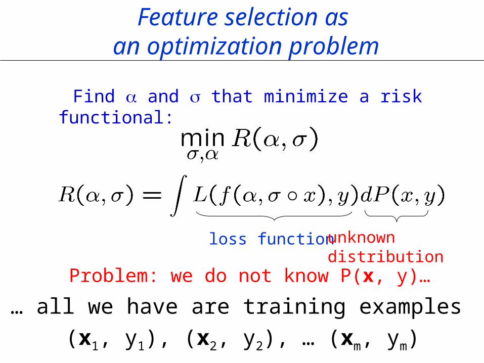
Feature selection as an optimization problem
Find and that minimize a risk functional:
Problem: we do not know P(x, y)…
loss function unknown distribution
… all we have are training examples
(x1, y1), (x2, y2), … (xm, ym)
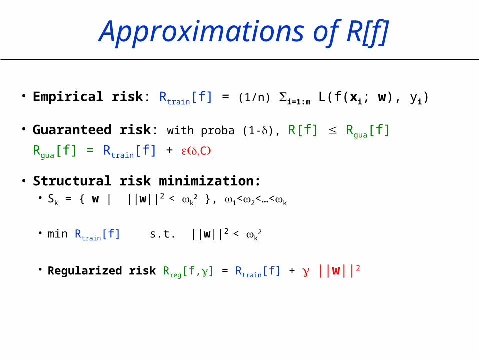
Approximations of R[f]
• Empirical risk: Rtrain[f] = (1/n) i=1:m L(f(xi; w), yi)
• Guaranteed risk: with proba (1-), R[f] Rgua[f]
Rgua[f] = Rtrain[f] + C
• Structural risk minimization: • Sk = { w | ||w||2 < k
2 }, 1<2<…<k
• min Rtrain[f] s.t. ||w||2 < k2
• Regularized risk Rreg[f,] = Rtrain[f] + ||w||2
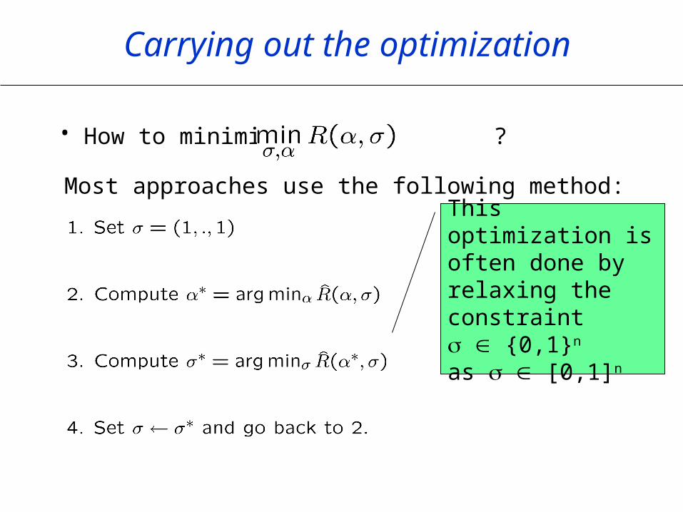
Carrying out the optimization
• How to minimize ?
Most approaches use the following method:
This optimization is often done by relaxing the constraint {0,1}n as [0,1]n
Add/Remove features 1
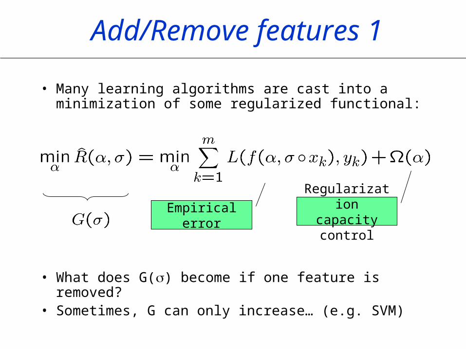
• Many learning algorithms are cast into a minimization of some regularized functional:
• What does G() become if one feature is removed?• Sometimes, G can only increase… (e.g. SVM)
Empirical errorRegularization
capacity control
Add/Remove features 2
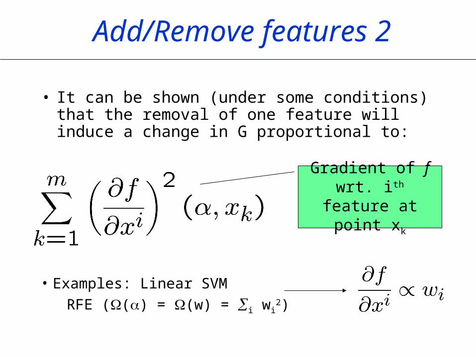
• It can be shown (under some conditions) that the removal of one feature will induce a change in G proportional to:
• Examples: Linear SVM
RFE (() = (w) = i wi2)
Gradient of f wrt. ith feature at point xk
Add/Remove features - RFE
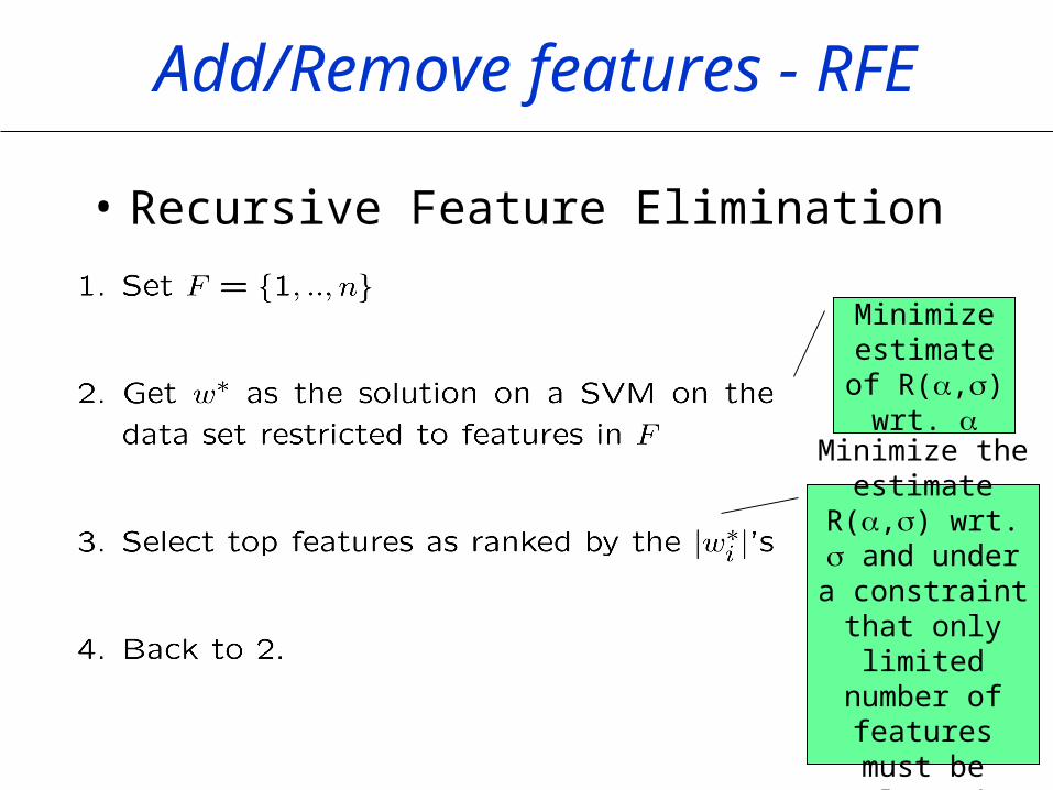
• Recursive Feature Elimination
Minimize estimate of
R(,) wrt.
Minimize the estimate R(,) wrt. and under a constraint that
only limited number of
features must be selected
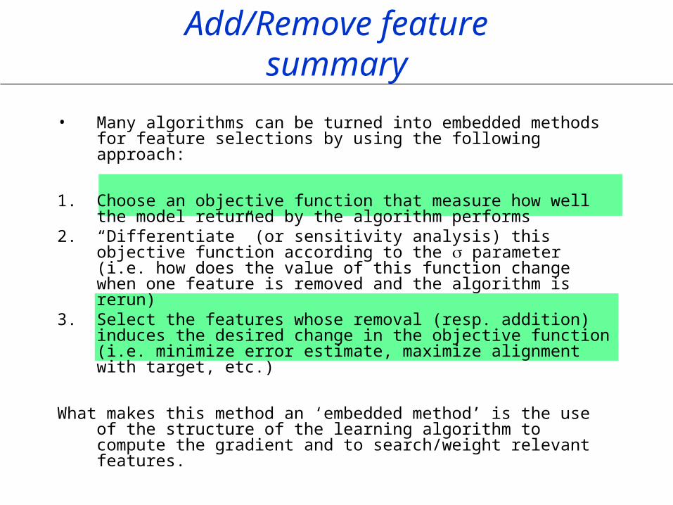
Add/Remove featuresummary
• Many algorithms can be turned into embedded methods for feature selections by using the following approach:
1. Choose an objective function that measure how well the model returned by the algorithm performs
2. “Differentiate” (or sensitivity analysis) this objective function according to the parameter (i.e. how does the value of this function change when one feature is removed and the algorithm is rerun)
3. Select the features whose removal (resp. addition) induces the desired change in the objective function (i.e. minimize error estimate, maximize alignment with target, etc.)
What makes this method an ‘embedded method’ is the use of the structure of the learning algorithm to compute the gradient and to search/weight relevant features.
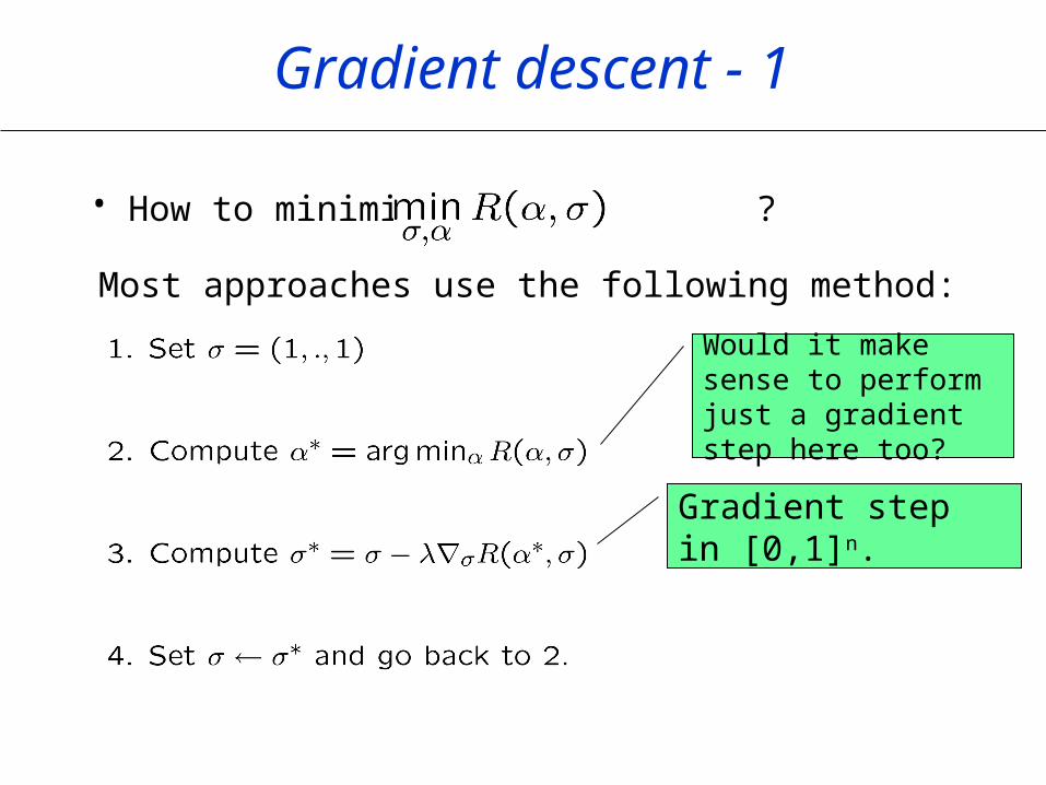
Gradient descent - 1
• How to minimize ?
Most approaches use the following method:
Gradient step in [0,1]n.
Would it make sense to perform just a gradient step here too?
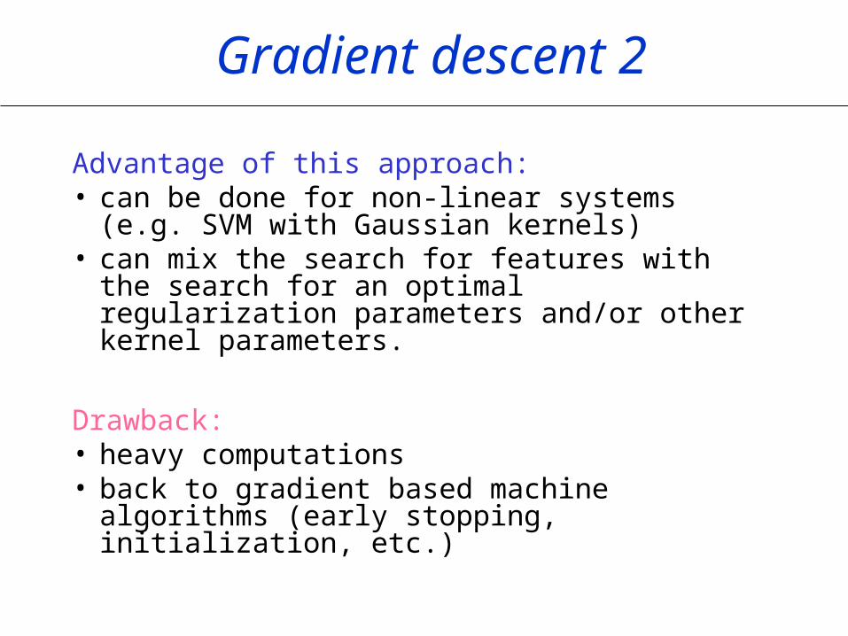
Gradient descent 2
Advantage of this approach: • can be done for non-linear systems (e.g. SVM
with Gaussian kernels)• can mix the search for features with the
search for an optimal regularization parameters and/or other kernel parameters.
Drawback: • heavy computations• back to gradient based machine algorithms
(early stopping, initialization, etc.)
Gradient descentsummary
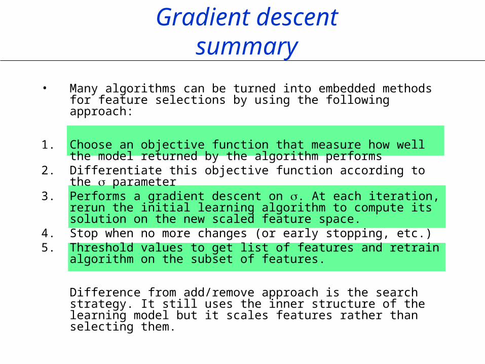
• Many algorithms can be turned into embedded methods for feature selections by using the following approach:
1. Choose an objective function that measure how well the model returned by the algorithm performs
2. Differentiate this objective function according to the parameter
3. Performs a gradient descent on . At each iteration, rerun the initial learning algorithm to compute its solution on the new scaled feature space.
4. Stop when no more changes (or early stopping, etc.)5. Threshold values to get list of features and retrain algorithm
on the subset of features.
Difference from add/remove approach is the search strategy. It still uses the inner structure of the learning model but it scales features rather than selecting them.
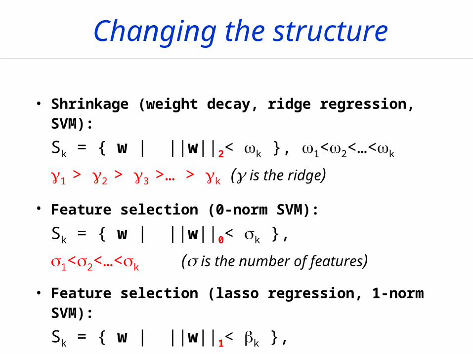
Changing the structure
• Shrinkage (weight decay, ridge regression, SVM):
Sk = { w | ||w||2< k }, 1<2<…<k
1 > 2 > 3 >… > k ( is the ridge)
• Feature selection (0-norm SVM):
Sk = { w | ||w||0< k },
1<2<…<k ( is the number of features)
• Feature selection (lasso regression, 1-norm SVM):
Sk = { w | ||w||1< k },
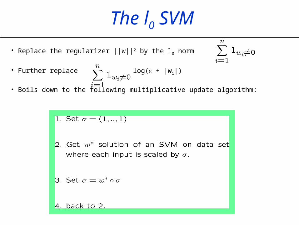
• Replace the regularizer ||w||2 by the l0 norm
• Further replace by i log( + |wi|)
• Boils down to the following multiplicative update algorithm:
The l0 SVM
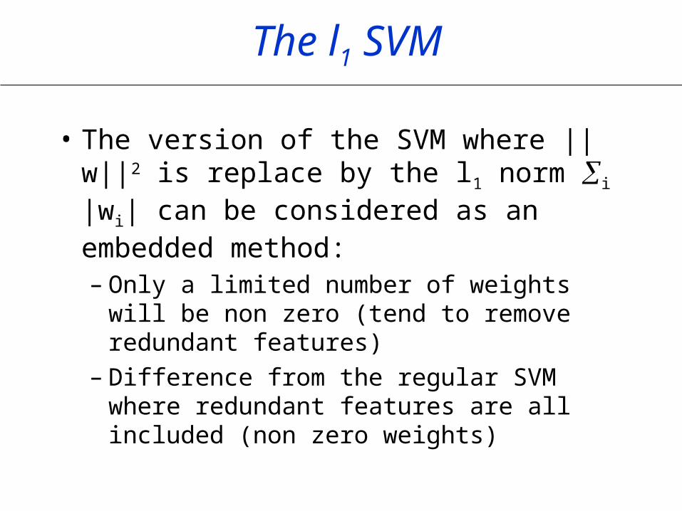
The l1 SVM
• The version of the SVM where ||w||2 is replace by the l1 norm i |wi| can be considered as an embedded method:– Only a limited number of weights will be
non zero (tend to remove redundant features)
– Difference from the regular SVM where redundant features are all included (non zero weights)
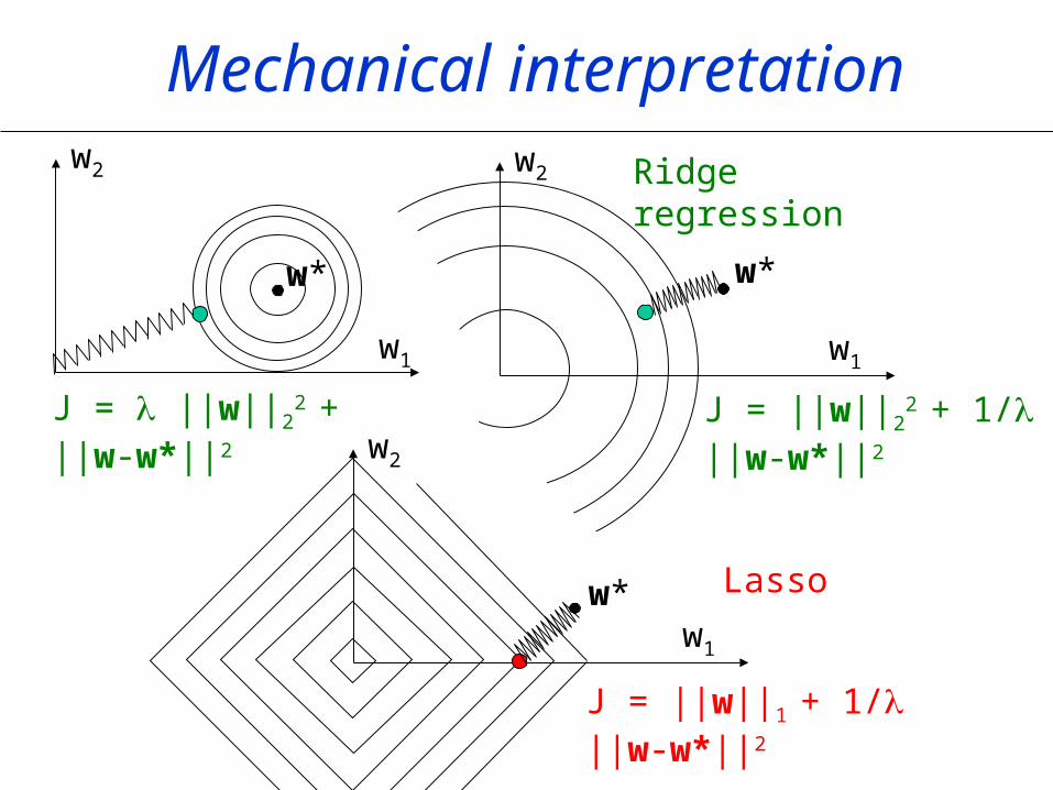
Ridge regression
w1
w2
w*
J = ||w||22 + 1/ ||w-w*||2
Mechanical interpretationw2
J = ||w||22 + ||w-w*||2
w*
w1
w1
w2
w*
J = ||w||1 + 1/ ||w-w*||2
Lasso
Embedded method - summary
• Embedded methods are a good inspiration to design new feature selection techniques for your own algorithms:– Find a functional that represents your prior knowledge about
what a good model is.– Add the weights into the functional and make sure it’s
either differentiable or you can perform a sensitivity analysis efficiently
– Optimize alternatively according to and – Use early stopping (validation set) or your own stopping
criterion to stop and select the subset of features
• Embedded methods are therefore not too far from wrapper techniques and can be extended to multiclass, regression, etc…
Feature Extraction, Foundations and ApplicationsI. Guyon et al, Eds.Springer, 2006.http://clopinet.com/fextract-book
Book of the NIPS 2003 challenge