Lecture 4: Propagation Models, Antennas and Link

BudgetAnders Västberg

vastberg@kth.se

08-790 44 55

Digital Communication System

Source of Information

SourceEncoder

Modulator RF-Stage

Channel

RF-StageInformation

SinkSource

DecoderDemodulator

ChannelEncoder

DigitalModulator

ChannelDecoder

DigitalDemodulator

[Slimane]

Propagation between two antennas (not to scale)

No Ground Wave for Frequencies > ~2 MHzNo Ionospheric Wave for Frequencies > ~30 Mhz

Direct Wave

Ground ReflectedWave

Ground Wave

Sky Wave

The Radio Link

• Design considerations– The distance over which the system meets

the performance objectives– The capacity of the link.

• Performance determined by– Frequency– Transmitted Power– Antennas– Technology used

[Black et. al]

Performance of Radio Systems

• Signal attenuation– path loss– multipath fading

• Additive noise– Thermal noise– Atmospheric noise– Cosmic Noise– Man-made noise

Noise

• Thermal noise – White Noise• Spectral density: (W/Hz)

k Boltzmann’s constant (1.38 10-23 J/K)T Absolute temperature (in Kelvins)

• Noise power (in W)

B Bandwidth (Hz)

TBkN

TkN 0

Signal to noise ratio (SNR)

• Ratio between signal power and noise power

Link Budget

𝑃𝑟=𝑃 𝑡 ∙𝐺𝑡 ∙𝐺𝑟

𝐿𝑏

PtG

tP

rL

b

r

Gr

SNR=𝑃𝑟

𝑁=𝑃𝑡 ∙𝐺𝑡 ∙𝐺𝑟

𝑁 𝐿𝑏

=𝑃 𝑡 ∙𝐺𝑡 ∙𝐺𝑟

𝑘𝑇0𝐵𝐿𝑏

SNR𝑑𝐵=(𝑃 ¿¿𝑡)𝑑𝐵+(𝐺¿¿𝑡)𝑑𝐵−(𝐿¿¿𝑏)𝑑𝐵+(𝐺¿¿𝑟 )𝑑𝐵−(𝑘𝑇 ¿¿ 0𝐵)𝑑𝐵¿¿¿¿¿

𝑃 𝐸𝐼𝑅𝑃=𝑃𝑡 ∙𝐺𝑡

EIRP=Effective Isotropic Radiated Power

Propagations Models

𝐿𝐹𝑆=( 4 𝜋𝑟𝜆 )2

=( 4𝜋 𝑓 𝑟𝑐 )

2

Free Space Model

𝐿𝑃𝐸=𝑟4

(h1h2 )2Plane Earth Model

𝐿=𝑟𝑛

𝑘Power Law Model

Dipole antennaOmnidirectional

L= /2l

I I

• Half-wave dipole– Gain 1,64 = 2.15 dBi– Linear Polarisation

• Quarter-wave dipole– Conducting plane below a

single quarter wave antenna. Acts like a half-wave dipole

L=l/4

I

Yagi-antennaDirectional

http://www.urel.feec.vutbr.cz/~raida/multimedia_en/chapter-4/4_3A.html

3-30 element and a gain of 8-20 dBi

Parabolic antennaDirectional

• Effective area

Ae = hp d2/4

=0.56h

[Stallings, 2005]

Corner Reflectors

• Multiple images results in increased gain

• Example:G=12 dBi

/2l

Driven Element

Images

Loop-antenna - Directional

http://www.ycars.org/EFRA/Module%20C/AntLoop.htm

• Linear Polarisation

• Gain 1,76 dBi

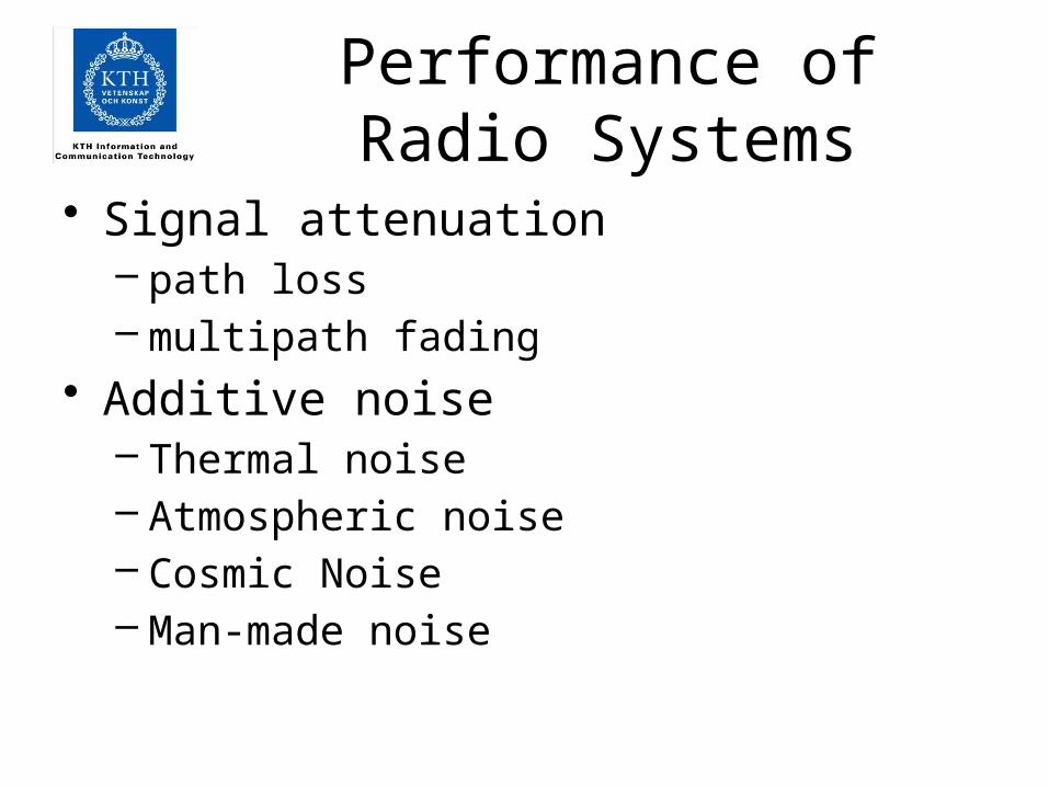
Helical antennaDirectional

• Normal mode• Axial mode

http://hastingswireless.homeip.net/index.php?page=antennas&type=helical

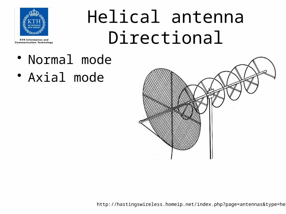
Microwave Communication

[Slimane]

Propagation in the Atmosphere

• The atmosphere around the earth contains a lot of gases (1044 molecules)

• It is most dense at the earth surface (90% of molecules below a height of 20 km).

• It gets thinner as we reach higher and higher attitudes.

• The refractive index of the air in the atmosphere changes with the Height

• This affects the propagation of radio waves.• The straight line propagation assumption may

not be valid especially for long distances.

[Slimane]

Effective Earth Radius

[Slimane]

Line-of-Sight Range

[Slimane]

Ray Paths and Wave fronts

Fresnel Zone

[Slimane]

Ionospheric Communication

[Davies, 1993]

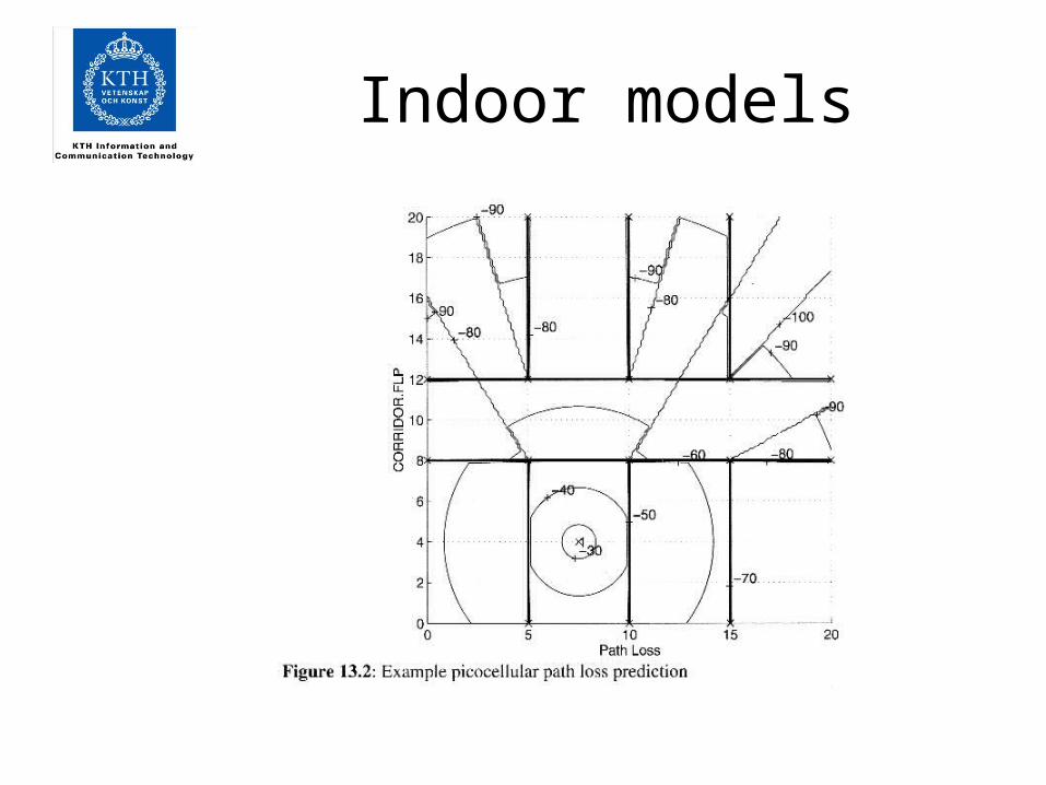
Indoor models

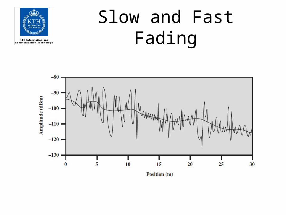
Slow and Fast Fading

Homework before F6

• Describe the following modulation methods:– AM, FSK, BPSK, QAM

• Order ASK, FSK, PSK and DPSK in order of least efficient to most efficient.