Lecture 5 Multiple Choice Models Part I –MNL, Nested Logit · PDF fileRS – Lecture 17 1 Lecture 5 Multiple Choice Models Part I –MNL, Nested Logit DCM: Different Models •Popular

RS – Lecture 17

1

Lecture 5

Multiple Choice Models

Part I – MNL, Nested Logit

DCM: Different Models

• Popular Models:

1. Probit Model

2. Binary Logit Model

3. Multinomial Logit Model

4. Nested Logit model

5. Ordered Logit Model

• Relevant literature:

- Train (2003): Discrete Choice Methods with Simulation

- Franses and Paap (2001): Quantitative Models in Market Research

- Hensher, Rose and Greene (2005): Applied Choice Analysis

RS – Lecture 17

Multinomial Logit (MNL) Model

• In many of the situations, discrete responses are more complex than the binary case:

- Single choice out of more than two alternatives: Electoral choices and interest in explaining the vote for a particular party.

- Multiple choices: “Travel to work in rush hour,” and “travel to work out of rush hour,” as well as the choice of bus or car.

• The distinction should not be exaggerated: we could always enumerate travel-time, travel-mode choice combinations and then treat the problem as making a single decision.

• In a few cases, the values associated with the choices will themselves be meaningful, for example, number of patents: y = 0; 1,2,... (count data). In most cases, the values are meaningless.


• In most cases, the value of the dependent variable is merely a coding for some qualitative outcome:

- Labor force participation: we code “yes" as 1 and “no" as 0

(qualitative choices)

- Occupational field: 0 for economist, 1 for engineer, 2 for lawyer, etc. (categories)

- Opinions are usually coded with scales, where 1 stands for “strongly disagree", 2 for “disagree", 3 for “neutral", etc.

• Nothing conceptually difficult about moving from a binary to a multi-response framework, but numerical difficulties can be big.

• A simple model to generalized: The Logit Model.

RS – Lecture 17


• Now, we have a choice between J (greater than 2) categories

• Dependent variable yn = 1, 2, 3, .... J

• Explanatory variables

– zn, different across individuals, not across choices (standard MNL model). The MLN specifies for choice j = 1,2,..., J:

– xn, different across (individuals and) choices (conditional MNLmodel). The conditional logit model specifies for choice j:

• Both models are easy to estimate.

∑+===

l l

j

nnz

zzzjyP

)'exp(1

)'exp()|(

α

α

∑==

l jn

jn

nnx

xxjyP

)'exp(

)'exp()|(

β

β


• The MNL can be viewed as a special case of the conditional logitmodel. Suppose we have a vector of individual characteristics Zi of dimension K, and J vectors of coefficients αj, each of dimension K. Then define,

• We are back in the conditional logit model.

RS – Lecture 17

MNL – Link with Utility Maximization

• The modeling approach (McFadden’s) is similar to the binary case.

- Random Utility for individual n, associated with choice j:

Un1 = Vnj+ εnj = αj+z’n δj+w’n γj + εnj - utility from decision j

- same parameters for all n.Then, if yn = j if (Unj - Uni) > 0 (n selects j over i.)

- Like in the binary case, we get:

- Specify i.i.d. Gumbel distribution for f(ε) => Logit Model.

- independence across utility functions

- identical variances (means absorbed in constants)

nnninjn

ninjnjninni

dfijVVI

ijVVjijyP

ξξ≠∀−<ξ=

≠∀−<ε−ε===

∫ )()(

)(Prob],|[Prob

• If we add a constant to a parameter (βi +c), given the Logistic distribution, exp(c) will cancel out. Cannot distinguish between (βi +c)

and βi . Need a normalization ⇒ select a reference category, say i, and set coefficients equal to 0 –i.e., βi=0. (Typically, i=J.)

• Conditional MNL model (xn: different across (individuals and) choices)

∑==

l nl

nj

nnx

xxjyP

)'exp(

)'exp()|(

β

β

ijx

xxjyP

xxiyP

il nl

nj

nn

il nl

nn

≠∀+

==

+==

∑

∑

≠

≠

)'exp(1

)'exp()|(

)'exp(1

1)|(

β

β

β

∑==

l nl

nj

nnx

xxjyP

)'exp(

)'exp()|(

β

β

MNL Model - Identification

RS – Lecture 17

•The interpretation of parameters is based on partial effects:

– Derivative (marginal effect)

– Elasticity (proportional changes)

Note: The elasticity is the same for all choices “j.” A change in the cost of air travel has the same effect on all other forms of travel. (This result is called independecne from irrelevant alternatives (IIA). Not a realistic property. Many experiments reject it.)

knjnjnk

nn PPx

xjyPβ−=

∂

=∂)1(

)|(

knjnk

knjnj

nj

nk

nk

nj

Px

PPP

x

x

P

β−=

β−=∂

∂

)1(

)1(log

log

MNL Model – Interpretation & Effects

• Interpretation of parameters

– Probability-ratio

– Does not depend on the other alternatives! A change in attribute xnk does not affect the log-odds ratio between choices j and i. This result is called independence from irrelevant alternatives (IIA). Implication of MNL models pointed out by Luce (1959).

Note: The log-odds ratio of each response follow a linear model. A regression can be used for the comparison of two choices at a time.

)(')|(

)|(ln

)'exp(

)'exp(

)|(

)|(

ninj

nn

nn

ni

nj

nn

nn

xxxiyP

xjyP

x

x

xiyP

xjyP

−=

=

=

==

=

β

β

β

MNL Model – Interpretation & Effects

RS – Lecture 17

• Estimation

– ML estimation

))'exp(ln())'((

)))'exp(ln()'exp((ln(

)'exp(

)'exp(ln)(

)|(ln)(

)|()(

∑∑ ∑

∑∑ ∑

∑∑ ∑

∑∑

∏∏

β−β=

β−β=

β

β=β

==β

==β

knjnj

n j

nj

knjnj

nj

nj

n j knj

nj

nj

n j

nnnj

n j

D

nn

xxD

xxD

x

xDLogL

xjyPDLogL

xjyPL nj

where Dnj=1 if j is selected, 0 otherwise)

MNL Model – Estimation

• Estimation

- ML:

A lot of f.o.c. equations, with a lot of unknowns (parameters).

Each covariate has J-1 coefficients.

We use numerical procedures, G-N or N-R often work well.

- Alternative estimation procedures

Simulation-assisted estimation (Train, Ch.10)

Bayesian estimation (Train, Ch.12)

MNL Model – Estimation

RS – Lecture 17

• Example (from Bucklin and Gupta (1992)):

• Ui = constant for brand-size i

– BLhi = loyalty of household h to brand of brandsize i

– LBPhit = 1 if i was last brand purchased, 0 otherwise

– SLhi = loyalty of household h to size of brandsize i

– LSPhit = 1 if i was last size purchased, 0 otherwise

– Priceit = actual shelf price of brand-size i at time t

– Promoit = promotional status of brand-size i at time t

itith

ithi

hit

hii

hit

j

hjt

hith

t

LSPSLLBPBLuU

U

UinciP

PromoPrice

)exp(

)exp()|(

654321 β+β+β+β+β+β+=

=∑

MNL Model – Application - PIM

• Data

– A.C.Nielsen scanner panel data

– 117 weeks: 65 for initialization, 52 for estimation

– 565 households: 300 selected randomly for estimation, remaining hh = holdout sample for validation

– Data set for estimation: 30,966 shopping trips, 2,275 purchases in the category (liquid laundry detergent)

– Estimation limited to the 7 top-selling brands (80% of category purchases), representing 28 brand-size combinations (= level of analysis for the choice model)


RS – Lecture 17

6061.6

3914.3

-

.364

-5957.3

-3786.9

27

33

Null model

Full model

BICU² (pseudo R²)LL# param.Model

• Goodness-of-Fit


3.499 (22.74)

.548 (6.50)

2.043 (13.67)

.512 (7.06)

-.696 (-13.66)

2.016 (21.33)

BL β1

LBP β2

SL β3

LSP β4

Price β5

Promo β6

Coefficients (t-statistic)Parameter

• Estimation Results

MNL Model – Application – Travel Mode

• Data: 4 Travel Modes: Air, Bus, Train, Car. N=210

-----------------------------------------------------------

Discrete choice (multinomial logit) model

Dependent variable Choice

Log likelihood function -256.76133

Estimation based on N = 210, K = 7

Information Criteria: Normalization=1/N

Normalized Unnormalized

AIC 2.51201 527.52265

Fin.Smpl.AIC 2.51465 528.07711

Bayes IC 2.62358 550.95240

Hannan Quinn 2.55712 536.99443

R2=1-LogL/LogL* Log-L fncn R-sqrd R2Adj

Constants only -283.7588 .0951 .0850

Chi-squared[ 4] = 53.99489

Prob [ chi squared > value ] = .00000

Response data are given as ind. choices

Number of obs.= 210, skipped 0 obs

--------+--------------------------------------------------

Variable| Coefficient Standard Error b/St.Er. P[|Z|>z]

--------+--------------------------------------------------

GC| .03711** .01484 2.500 .0124

INVC| -.05480*** .01668 -3.285 .0010

INVT| -.00896*** .00215 -4.162 .0000

HINCA| .02922*** .00931 3.138 .0017

A_AIR| -1.88740*** .69281 -2.724 .0064

A_TRAIN| .69364*** .25010 2.773 .0055

A_BUS| -.20307 .24817 -.818 .4132

--------+--------------------------------------------------

RS – Lecture 17

CLOGIT Fit Measure:

• Based on the log likelihood

• Based on the model predictions+------------------------------------------------------+

| Cross tabulation of actual vs. predicted choices. |

| Row indicator is actual, column is predicted. |

| Predicted total is F(k,j,i)=Sum(i=1,...,N) P(k,j,i). |

| Column totals may be subject to rounding error. |

+------------------------------------------------------+

Matrix Crosstab has 5 rows and 5 columns.

AIR TRAIN BUS CAR Total

+----------------------------------------------------------------------

AIR | 35.0000 (16) 7.0000 4.0000 13.0000 58.0000

TRAIN | 7.0000 41.0000 (19) 4.0000 11.0000 63.0000

BUS | 5.0000 4.0000 16.0000 (4) 4.0000 30.0000

CAR | 11.0000 11.0000 6.0000 31.0000 (17) 59.0000

Total | 58.0000 63.0000 30.0000 59.0000 210.0000

Values in parentheses below show the number of correct predictions by a model with only choice specific constants.


Constants only -283.7588 .0951 .0850

Chi-squared[ 4] = 53.99489

MNL Model – Application – Travel Mode

• Scale parameter

• Variance of the extreme value distribution Var[ε] = π²/6

- If true utility is U*nj = β

*’xnj + ε*nj with Var(ε

*nj)= σ² (π²/6), the

estimated representative utility Vnj = β’xnj involves a rescaling of β*

=> β= β* / σ

• β* and σ can not be estimated separately

⇒ Take into account that the estimated coefficients indicate the variable’s effect relative to the variance of unobserved factors

⇒ Include scale parameters if subsamples in a pooled estimation (may) have different error variances

MNL Model – Scaling

RS – Lecture 17

• Scale parameter in the case of pooled estimation of subsamples with different error variance

• For each subsamples, multiply utility by µs, which is estimated simultaneously with β

• Normalization: set µs equal to 1 for 1 subs.

• Values of µs reflect diff’s in error variation

– µs>1 : error variance is smaller in s than in the reference subsample

– µs<1 : error variance is larger in s than in the reference subsample

MNL Model – Scaling

• Example (from Breugelmans et al (2005), based on Andrews and Currim (2002); Swait and Louvière (1993)):

• Data from online experiment, 2 product categories• Three different assortments, assigned to different respondent groups– Assortment 1: small assortment– Assortment 2 = ass.1 extended with addirional brands– Assortment 3 = ass.1 extended with add types

• Explanatory variables are the same (hh char’s, MM), with exception of the constants

• A scale factor is introduced for assortment 2 and 3 (assortment 1 is reference with scale factor =1)

MNL Model – Application

RS – Lecture 17

Table 1: Descriptive stats for each assortment (margarine and cereals)

MARGARINE

Attribute Assortment 1

(limited)

Assortment 2 (add new

flavors of existing brands)


brands of existing flavors)Brand Common a Common Common

Add new brands

Flavor Common Common Common

Add new flavors

# alternatives 11 19 17

# respondents 105 116 100

# purchase occasions 275 279 278

# screens needed < 1 > 1 > 1

CEREALS

Attribute Assortment 1

(limited)


flavors of existing brands)


brands of existing flavors)Brand Common Common Common

Add new brands

Flavor Common Common Common

Add new flavors

# alternatives 21 32 46

# respondents 81 97 87

# purchase occasions 271 261 281

# screens needed > 1 > 1 > 1


• MNL-model – Pooled estimation

• Phit,a= the probability that household h chooses item i at time t, facing assortment a

• uhit,a= the choice utility of item i for household h facing assortment a= f(household variables, MM-variables)

• Cha= set of category items available to household h within assortment a

• µa = Gumbel scale factor

[ ][ ]∑

∈

=

haCj

h

ajta

h

aitah

aitu

up

)(exp

)(exp

|

|

|µ

µ


RS – Lecture 17

Estimation results

• Goodness-of-Fit

– (average) LL: -0.045 (M), -0.040 (C)

– BIC: 2929 (M), 4763(C)

– CAIC: 2871 (M), 4699 (C)

• Scale factors:

– M: 1.2498 (ass2), 1.2627 (ass3)

– C: 1.0562 (ass2), 0.7573 (ass3)


0.7573***[0.4888***]c

[3.9109***]c

0.0969-0.15960.3816**0.6190***4.1140***

1.0562***[0.6803***]c

[5.4934***]c

0.61300.2938**-0.0614-0.06950.7214

[1.00]b

0.6441***5.2011***0.0077-0.02600.3119-0.33112.0041***

Scale factorMean

Last purchaseItem preferenceBrand asymmetryTaste asymmetryType asymmetrySequenceProximity

1.2627***[2.6106***]c

[3.5747***]c

0.5400*0.0169-0.11900.6235

1.2498***[2.5840***]c

[3.5382***]c

0.4228**-0.08800.3672**1.0303***

[1.00]b

2.0675***2.8310***0.2805-0.0841- d

0.8332

Scale factorMean

Last purchaseItem preferenceBrand asymmetrySize asymmetrySequenceProximity

Assortment 3Assortment 2Assortment 1VariableAssortment 3Assortment 2Assortment 1 Variable

CerealsMargarine

(Excluding brand/size constants)


RS – Lecture 17

• Limitations of the MNL model:

– Independence of Irrelevant Alternatives or IIA (proportional substitution pattern): the relative odds between any two outcomes are independent of the number and nature of other outcomes being simultaneously considered.

– Order (where relevant) is not taken into account

– Systematic taste variation can be represented, not random taste variation

– No correlation between error terms (i.i.d. errors)

MNL Model – Limitations

• This is the big weakness of the model. The choice between any two alternatives does not depend upon a third one -i.e., the ratio of choice probabilities for alternatives i and j does not depend on characteristics of other alternatives, say, xi3.

• Implications: Proportional substitution patterns (or unrealistic substitution patterns!). It is possible to ignore third alternatives in estimation.

• But, it clashes with data

MNL Model – IIA

)'exp(

)'exp(

)|(

)|(

ini

jnj

nn

nn

x

x

xiyP

xjyP

β

β=

=

=

RS – Lecture 17

Example (McFadden (1974)): Blue Bus – Red Bus:

Suppose we have three equally distributed transportation categories:

- T1: Blue bus (P=33%), Car (P=33%), Red bus (P=33%)

Now, we paint the red busses blue. Then, we have two choices. Assuming IIA, we have: Blue bus (P=50%), Car (P=50%).

But, a more likely distribution: Blue bus (P=66%), Car (P=33%).

Note: Debreu (1960) has a similar example with Beethoven/Debussy.

• MNL model assumes that none of the categories can serve as substitutes (no correlation). If they can serve as substitutes, then the results of MNL may not be very realistic.

MNL Model – IIA

• We want to test IIA.

Hausman-McFadden specification test (Econometrica, 1983)

• Basic idea: If a subset of the choice set is truly irrelevant, omitting itshould not significantly affect the estimates. Two estimators: one efficient, one inefficient => encompassing test.

Steps for Wald test:

- Estimate logit model twice:

(a) on full set of alternatives (with “irrelevant” variables)

(b) on subset of alternatives (and subsamples with choices from this set)

- Compute the Wald test

- Under H0 (IIA is true):

MNL Model – IIA - Testing

( ) ( ) ( ) )²(~1'

kbaabba χββββ −Ω−Ω−−

RS – Lecture 17

Steps for LR test:- Estimate logit model twice:

a. on full set of alternativesb. on subset of alternatives(and subsample with choices from this set)

- Compute LogL for subset (b) with parameters obtained for set (a) - Compare with LogLb: Goodness of fit should be similar

MNL Model – IIA - Testing

• In the MNL model we assumed independent εnj with extreme value distributions. This essentially created the IIA property.

• This is not completely correct, because other distributions for the unobserved, say with normal errors, we would not get IIA exactly, but something pretty close to it.

• The solution to the IIA problem is to relax the independence between the unobserved components of the latent utility, εi.

• There are a number of ways to go.

Model – IIA: Alternative Models

RS – Lecture 17

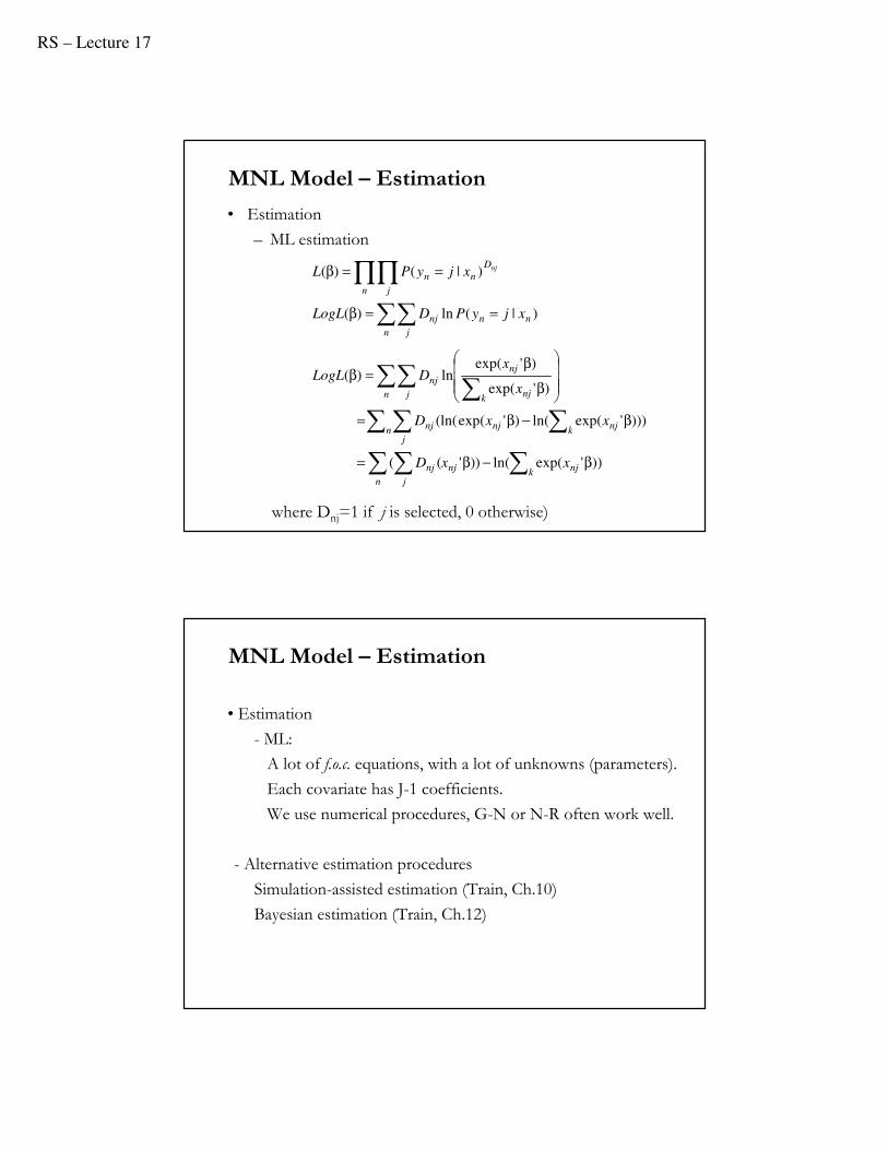
• Solutions to IIA

– Nested Logit Model, allowing correlation between some choices.

– Models that allow for correlation among the error terms, such as Multinomail Probit Models

– Mixed or random coefficients Logit, where the marginal utilities associated with choice characteristics are allowed to vary between individuals.

All of these originate in some form or another in McFadden’s work (1981, 1982, and 1984).

Model – IIA: Alternative Models

• We have J choices. We allow correlations between the choices through nesting them.

• We group together or cluster sets of choices into S sets: B1, B2,..., BS. We allow correlations between the choices through nesting them.

• Choices are correlated inside the nest (B1 (Bus nest) = red bus, blue bus). But, we force independence between the nests.

• Preferences as before: Individuals choosing the option with the highest utility, where the utility of choice j in set Bs for individual n is

Unj = xnj’ β +Zs’α + εnjwhere Zs represents characteristics of the nests and εεεε follows a generalized extreme value (GEV).

Nested Logit Model

RS – Lecture 17

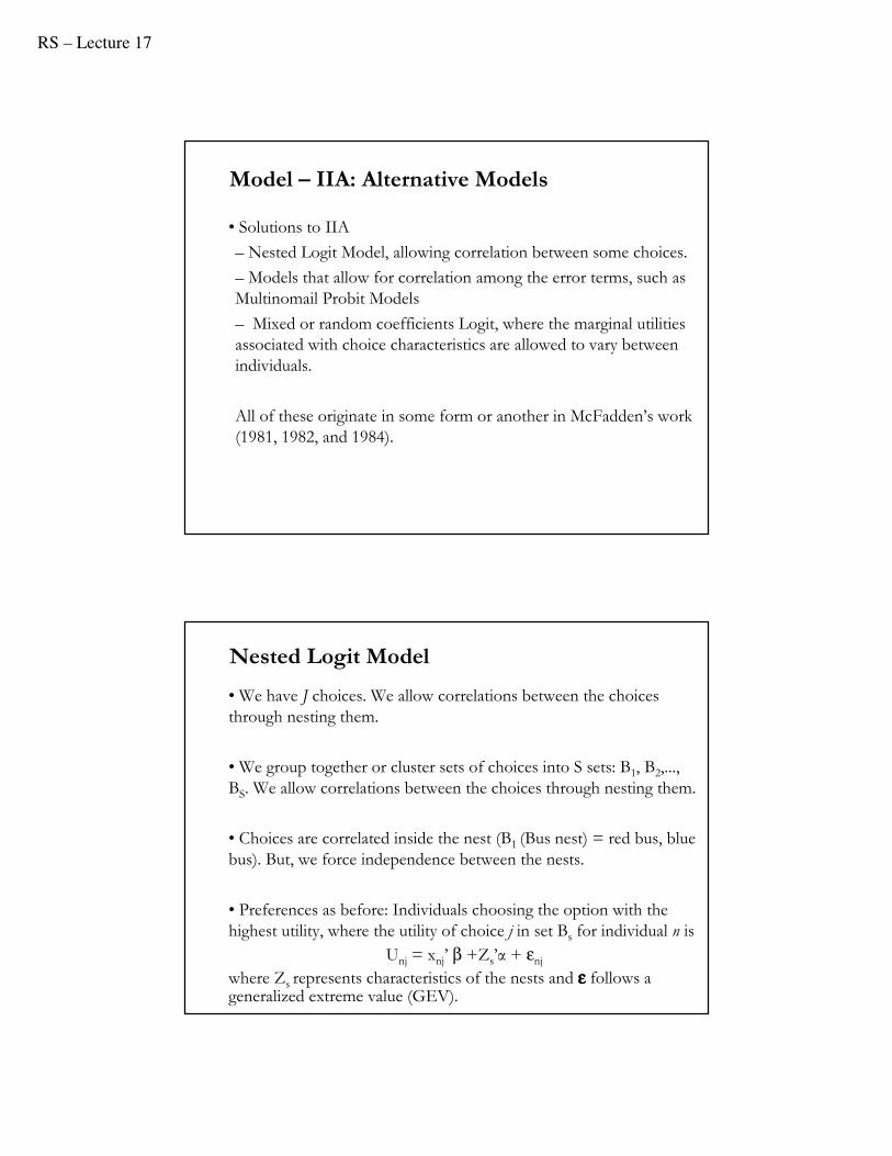
• εnj have a the joint cumulative distribution function of error terms is

• Within the sets the correlation coefficient for the εnj is approximately equal to 1− λ. Between the sets choices i & j are independent.

• Example: Transportation mode, with 4 choices: Bus, Train, Carpool & Car. We allow correlation among Bus & Train (εBus, εTraincorrelated) and among Car (alone) & Carpool (εCar, εCarpool correlated)

−=εεε

λ

= ∈

λε−∑ ∑s

s

snj

S

s Bj

nJnn eF

1

/

21 exp),...,,(

Nested Logit Model

Nested Logit Model - Probability

• The key in this model is how we form the nests. Different nest structures will produce different result.

• We choose the choices that are potentially close, with the data being used to estimate the amount of correlation.

RS – Lecture 17

Example: Transportation mode choice.

Choices: Bus, Train, Car (alone) & Carpool => J = 4.

• Nests: - Transit: Bus and Train

- Car: Car (alone) and Carpool

Choice of transportation mode

Transit Car

BusCar aloneTrain Carpool

Nested Logit Model - Example

LIMB

BRANCH

TWIG

Levels of Choice

• Example: Transportation mode choice.

Choices: Bus, Train, Car (alone) & Carpool => J = 4.

• No Nesting

Choice of transportation mode

Bus Car aloneTrain Carpool

Nested Logit Model - Example

Levels of Choice

Note: We are not assuming that individuals choose sequentially. The diagrams simply represents nesting patterns and structure of systemof logit models.

RS – Lecture 17

Nested Logit Model – Structure

• We cluster similar choices in nests or branches.

• The RUM as usual: Unj = Vni + εnj.

• But, it gets complicated. Now, we compound utility:

U(Choice) = U(Choice|Branch) + U(Branch)

- U(Branch) = function of some variables Z (characteristics of the branch, say comfort of ride, speed, price, etc).

- U(Choice|Branch) = function of some variables X (age, education, income). These variables vary across choices.

Nested Logit Model – Structure

• Within a branch

– Identical variances (IIA applies)

– Covariance (all same) = variance at higher level

• Branches have different variances (scale factors)

• Nested logit probabilities: Generalized Extreme Value

• Prob[Choice,Branch] = Prob(Branch) * Prob(Choice|Branch)

=> We need two models:

1) Model of branch selection

2) Model of Choice, given branch selection

RS – Lecture 17


• Let Zs be branch/set-specific characteristics. (It may be empty, an indicator variable for set S, etc.). This set influences your choice of branch.

• Let the conditional probability of choice j given that your choice is in the set Bs, or YnЄBs (“twig level probability”) be equal to:

for j ЄBs, and 0 otherwise.

This probability describes the lower level model –describes choice within the nest or at twig level, given a branch.

Unusual notation: Correlation inside the nest = 1 – λ, λ Є[0,1].

∑ ∈λ

λ=∈=

lBkSnk

Snj

snnnV

VBYXjYP

)/exp(

)/exp(],|[


• Suppose the marginal probability of each choice in the set Bs:

This is the upper level model –describes choices between nests (probability of a branch).

• If λs=1 for all s –i.e., no correlation within the nest-, then

• We are back to the conditional logit model.

∑ ∑=

∈

α+

α+=

S

lBk

lnk

snj

nj

l

ZV

ZVP

1

)'exp(

)'exp(

∑ ∑

∑

=

λ

∈

λ

∈

λα

λα

∈=S

lBk

lnkl

BkSnks

nsnnBsl

l

s

S

VZ

VZ

XBYPP

1

)/exp()'exp(

)/exp()'exp(

]|[

RS – Lecture 17

Nested Logit Model - Summary

• The nested logit probability can be decomposed into 2 logit models:

Pj = Prob[nest containing j] × Prob[j, given nest containing j]

∑∑

∑

∈

∈

λ=

λ+α

λ+α=

λ

λ=

=

k

k

k

k

kk

Bj

knjnk

lnllnl

nkknkBn

Bjknj

kniBni

BnBnini

VIV

IVZ

IVZP

V

VP

with

PPP

)/exp(ln

)'exp(

)'exp(

)/exp(

)/exp(

,

|

,|

(1) Lower level model

(2) Upper level model

• There is a link between Pni|Bk*Pn,Bk (upper and lower level): the inclusive value IVnk --the log of the denominator of lower level model.

(3) Inclusive value

• IVs is also called the log-sum for nest BS. It represents the expected utility for the choice of alternatives within nest BS.

IVBs = E[maxjЄBs Uj] = E[maxjЄBs (Vj + εj)]

• For consistency with RUM, λk must be in the [0,1] interval (sufficient condition) –see McFadden (1981). The value of λk can serve as a check on the nested logit model.

• IIA within, not across nests.

( )( ) 1

1

)/exp()/exp(

)/exp()/exp(

−

∈

−

∈

∑∑

=l

l

k

k

Bm lnmlnj

Bm knmkni

nj

ni

VV

VV

P

Pλ

λ

λλ

λλ

• When λk =1 => no correlation within nests: )exp(

)exp(

nj

ni

nj

ni

V

V

P

P=


RS – Lecture 17

Example: Transportation mode with 4 choices( Bus, Train, Car (alone) & Carpool) and 2 nests (Transit: Bus and Train; Car: Car (alone) and Carpool)

- Lower level model. It gives conditional probability of transit choices –conditional on choosing transit mode. For exampe, conditional probability of choosing Bus, conditional on choosing the Transit nest:

Similarly, conditional probability of choosing Carpool, conditional on choosing the Car nest:

)/'exp()/'exp(

)/'exp(],|[

TransitnTrainTransitnBus

TransitnBusTransitnnn

xx

xBYXBusYP

λβ+λβ

λβ=∈=

)/'exp()/'exp(

)/'exp(],|[

CaralonenCarCarnCarpool

CarnCarpool

Carnnnxx

xBYXCarpoolYP

λβ+λβ

λβ=∈=

−


Example (continuation).

Note: β enters into both equations => simultaneous estimation

- IIA holds within nests:

it depends on xbus and xTrain only.

- Inclusive value: Expected utility from choice given branch choice

)/'exp(

)/'exp(

],|[

],|[

TransitnTrain

TransitnBus

Transitnnn

Transitnnn

x

x

BYXTrainYP

BYXBusYP

λβ

λβ=

∈=

∈=

[ ][ ])/'exp()/'exp(ln

)/'exp()/'exp(ln

CaralonenCarCarnCarpoolCar

TransitnTrainTransitnBusTransit

xxIV

xxIV

λβ+λβ=

λβ+λβ=

−


RS – Lecture 17

Example (continuation).

- Upper level model. It gives the probability of choosing a nest/branch. For example, the probability of choosing Transit:

∑=

λ+α

λ+α=∈

BusTransitl

nlll

nTransitTransitnTransitnTransitn

IVZ

IVZXBYP

,

)'exp(

)'exp(]|[


Nested Logit Model - Estimation

• Estimation

- ML joint estimation.

Complicated, especially since the log likelihood function is notconcave, but it is not impossible. Convergence is not guaranteed.

- Sequential estimation using nesting structure

(1) Estimate lower model: Within the nest we have a conditional MNL with coefficients β/λs. (Easy to estimate, log likelihood is concave.)

(2) Compute inclusive value, ln(Σl exp(Vnl./λs), using the estimates of β/λs.

(3) Estimate upper model with inclusive value as explanatory variable: Plug the estimates of β/ λs in Pni. Another conditional MNL model.

RS – Lecture 17

Nested Logit Model - Estimation

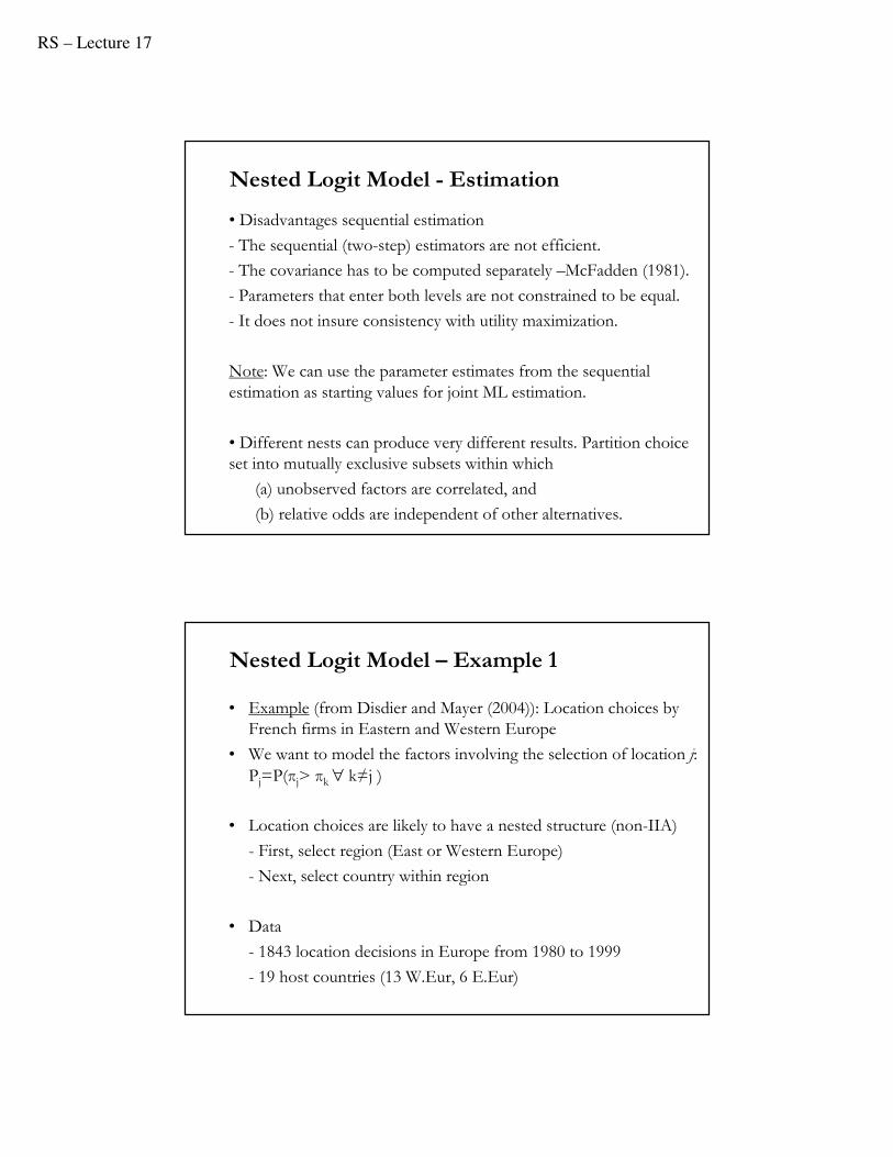
• Disadvantages sequential estimation

- The sequential (two-step) estimators are not efficient.

- The covariance has to be computed separately –McFadden (1981).

- Parameters that enter both levels are not constrained to be equal.

- It does not insure consistency with utility maximization.

Note: We can use the parameter estimates from the sequential estimation as starting values for joint ML estimation.

• Different nests can produce very different results. Partition choice set into mutually exclusive subsets within which

(a) unobserved factors are correlated, and

(b) relative odds are independent of other alternatives.

Nested Logit Model – Example 1

• Example (from Disdier and Mayer (2004)): Location choices by French firms in Eastern and Western Europe

• We want to model the factors involving the selection of location j:

Pj=P(πj> πk ∀ k≠j )

• Location choices are likely to have a nested structure (non-IIA)

- First, select region (East or Western Europe)

- Next, select country within region

• Data

- 1843 location decisions in Europe from 1980 to 1999

- 19 host countries (13 W.Eur, 6 E.Eur)

RS – Lecture 17


• Location choices: Data– NF French firms already located in the country– GDP GDP– GPP/CAP GDP per capita– DIST Distance France – host country– W Average wage per capita (manufacturing)– UNEMPL unemployment rate– EXCHR Exchange rate volatility– FREE Free country– PNFREE Partly free and not free country– PR1 Country with political rights rated 1– PR2 Country with political rights rated 2– PR345 Country with political rights rated 3,4,5– PR67 Country with political rights rated 6,7– LI Annual liberalization index– CLI Cumulative liberalization index– ASSOC =1 if an association agreement is signed

• Location choices by French firms in Eastern and Western Europe

Location choice

E.Eur

C1 CJ+1CJCN

W.Eur

……… ………


RS – Lecture 17



RS – Lecture 17


Example: Transportation mode (Air, train, bus, caaaaa)

STATA comands: NLOGIT

; Lhs=mode

; Rhs=gc,ttme,invt,invc

; Rh2=one,hinc

; Choices=air,train,bus,car

; Tree=Travel[Private(Air,Car), Public(Train,Bus)]

; Show tree

; Effects: invc(*)

; Describe

; RU1 $ (RU1: Random utility Model 1 – the one presented). This option selects branch normalization

Nested Logit Model – Example 2 (Greene)

RS – Lecture 17


• Tree Structure Specified for the Nested Logit ModelSample proportions are marginal, not conditional.

Choices marked with * are excluded for the IIA test.

----------------+----------------+----------------+----------------+------+---

Trunk (prop.)|Limb (prop.)|Branch (prop.)|Choice (prop.)|Weight|IIA

----------------+----------------+----------------+----------------+------+---

Trunk1 1.00000|TRAVEL 1.00000|PRIVATE .55714|AIR .27619| 1.000|

| | |CAR .28095| 1.000|

| |PUBLIC .44286|TRAIN .30000| 1.000|

| | |BUS .14286| 1.000|

----------------+----------------+----------------+----------------+------+---+---------------------------------------------------------------+

| Model Specification: Table entry is the attribute that |

| multiplies the indicated parameter. |

+--------+------+-----------------------------------------------+

| Choice |******| Parameter |

| |Row 1| GC TTME INVT INVC A_AIR |

| |Row 2| AIR_HIN1 A_TRAIN TRA_HIN3 A_BUS BUS_HIN4 |

+--------+------+-----------------------------------------------+

|AIR | 1| GC TTME INVT INVC Constant |

| | 2| HINC none none none none |

|CAR | 1| GC TTME INVT INVC none |

| | 2| none none none none none |

|TRAIN | 1| GC TTME INVT INVC none |

| | 2| none Constant HINC none none |

|BUS | 1| GC TTME INVT INVC none |

| | 2| none none none Constant HINC |

+---------------------------------------------------------------+


• STARTING VALUES-----------------------------------------------------------

Discrete choice (multinomial logit) model

Dependent variable Choice


Estimation based on N = 210, K = 10

R2=1-LogL/LogL* Log-L fncn R-sqrd R2Adj

Constants only -283.7588 .3905 .3787

Chi-squared[ 7] = 221.63022

Prob [ chi squared > value ] = .00000



--------+--------------------------------------------------


--------+--------------------------------------------------

GC| .07578*** .01833 4.134 .0000

TTME| -.10289*** .01109 -9.280 .0000

INVT| -.01399*** .00267 -5.240 .0000

INVC| -.08044*** .01995 -4.032 .0001

A_AIR| 4.37035*** 1.05734 4.133 .0000

AIR_HIN1| .00428 .01306 .327 .7434

A_TRAIN| 5.91407*** .68993 8.572 .0000

TRA_HIN3| -.05907*** .01471 -4.016 .0001

A_BUS| 4.46269*** .72333 6.170 .0000

BUS_HIN4| -.02295 .01592 -1.442 .1493

--------+--------------------------------------------------

RS – Lecture 17

Nested Logit Model – Example 2 (Greene)• FIML Nested Multinomial Logit ModelDependent variable MODE


The model has 2 levels.

Random Utility Form 1: IVparms = LMDAb|l


--------+--------------------------------------------------


--------+--------------------------------------------------

|Attributes in the Utility Functions (beta)

GC| .06579*** .01878 3.504 .0005

TTME| -.07738*** .01217 -6.358 .0000

INVT| -.01335*** .00270 -4.948 .0000

INVC| -.07046*** .02052 -3.433 .0006

A_AIR| 2.49364** 1.01084 2.467 .0136

AIR_HIN1| .00357 .01057 .337 .7358

A_TRAIN| 3.49867*** .80634 4.339 .0000

TRA_HIN3| -.03581*** .01379 -2.597 .0094

A_BUS| 2.30142*** .81284 2.831 .0046

BUS_HIN4| -.01128 .01459 -.773 .4395

|IV parameters, lambda(b|l),gamma(l)

PRIVATE| 2.16095*** .47193 4.579 .0000

PUBLIC| 1.56295*** .34500 4.530 .0000

|Underlying standard deviation = pi/(IVparm*sqr(6)

PRIVATE| .59351*** .12962 4.579 .0000

PUBLIC| .82060*** .18114 4.530 .0000

Nested Logit Model – Example 2 (Greene)+-----------------------------------------------------------------------+

| Elasticity averaged over observations. |

| Attribute is INVC in choice AIR |

| Decomposition of Effect if Nest Total Effect|

| Trunk Limb Branch Choice Mean St.Dev|

| Branch=PRIVATE |

| * Choice=AIR .000 .000 -2.456 -3.091 -5.547 3.525 |

| Choice=CAR .000 .000 -2.456 2.916 .460 3.178 |

| Branch=PUBLIC |

| Choice=TRAIN .000 .000 3.846 .000 3.846 4.865 |

| Choice=BUS .000 .000 3.846 .000 3.846 4.865 |

+-----------------------------------------------------------------------+

| Attribute is INVC in choice CAR |

| Branch=PRIVATE |

| Choice=AIR .000 .000 -.757 .650 -.107 .589 |

| * Choice=CAR .000 .000 -.757 -.830 -1.587 1.292 |

| Branch=PUBLIC |

| Choice=TRAIN .000 .000 .647 .000 .647 .605 |

| Choice=BUS .000 .000 .647 .000 .647 .605 |

+-----------------------------------------------------------------------+

| Attribute is INVC in choice TRAIN |

| Branch=PRIVATE |

| Choice=AIR .000 .000 1.340 .000 1.340 1.475 |

| Choice=CAR .000 .000 1.340 .000 1.340 1.475 |

| Branch=PUBLIC |

| * Choice=TRAIN .000 .000 -1.986 -1.490 -3.475 2.539 |

| Choice=BUS .000 .000 -1.986 2.128 .142 1.321 |

+-----------------------------------------------------------------------+

| Attribute is INVC in choice BUS |

| Branch=PRIVATE |

| Choice=AIR .000 .000 .547 .000 .547 .871 |

| Choice=CAR .000 .000 .547 .000 .547 .871 |

| Branch=PUBLIC |

| Choice=TRAIN .000 .000 -.841 .888 .047 .678 |

| * Choice=BUS .000 .000 -.841 -1.469 -2.310 1.119 |

+-----------------------------------------------------------------------+

| Effects on probabilities of all choices in the model: |

| * indicates direct Elasticity effect of the attribute. |

+-----------------------------------------------------------------------+

RS – Lecture 17

NL Model: Higher Level Trees (Greene)

• We can do higher order nesting. For example, housing choices can be divided by Location (Neighborhood); Housing Type (Rent, Buy, House, Apt); and Housing (# Bedrooms).

NL Model: Degenerate Branches (Greene)

Travel

Fly Ground

Air CarTrain Bus

BRANCH

TWIG

LIMB

• The branches do not have to have twigs. We can degenerate trees.

RS – Lecture 17

NL Model: Degenerate Branch (Greene)

• FIML Nested Multinomial Logit ModelDependent variable MODE


--------+--------------------------------------------------


--------+--------------------------------------------------


GC| .44230*** .11318 3.908 .0001

TTME| -.10199*** .01598 -6.382 .0000

INVT| -.07469*** .01666 -4.483 .0000

INVC| -.44283*** .11437 -3.872 .0001

A_AIR| 3.97654*** 1.13637 3.499 .0005

AIR_HIN1| .02163 .01326 1.631 .1028

A_TRAIN| 6.50129*** 1.01147 6.428 .0000

TRA_HIN2| -.06427*** .01768 -3.635 .0003

A_BUS| 4.52963*** .99877 4.535 .0000

BUS_HIN3| -.01596 .02000 -.798 .4248

|IV parameters, lambda(b|l),gamma(l)

FLY| .86489*** .18345 4.715 .0000

GROUND| .24364*** .05338 4.564 .0000


FLY| 1.48291*** .31454 4.715 .0000

GROUND| 5.26413*** 1.15331 4.564 .0000

--------+--------------------------------------------------

• STATA commands:NLOGIT ; lhs=mode

; rhs=gc,ttme,invt,invc; rh2=one,hinc; choices=air,train,bus,car; tree=Travel[Fly(Air),

Ground(Train,Car,Bus)]; show tree; effects:gc(*) ; Describe ; ru2 $

(This is RANDOM UTILITY FORM 2. The different normalization shows the effect of the degenerate branch.)


RS – Lecture 17

• Estimation of RU2 Form of Nested Logit Model

FIML Nested Multinomial Logit ModelDependent variable MODE

Log likelihood function -168.81283 (-148.63860 with RU1)

--------+--------------------------------------------------


--------+--------------------------------------------------


GC| .06527*** .01787 3.652 .0003

TTME| -.06114*** .01119 -5.466 .0000

INVT| -.01231*** .00283 -4.354 .0000

INVC| -.07018*** .01951 -3.597 .0003

A_AIR| 1.22545 .87245 1.405 .1601

AIR_HIN1| .01501 .01226 1.225 .2206

A_TRAIN| 3.44408*** .68388 5.036 .0000

TRA_HIN2| -.02823*** .00852 -3.311 .0009

A_BUS| 2.58400*** .63247 4.086 .0000

BUS_HIN3| -.00726 .01075 -.676 .4993

|IV parameters, RU2 form = mu(b|l),gamma(l)

FLY| 1.00000 ......(Fixed Parameter)......

GROUND| .47778*** .10508 4.547 .0000


FLY| 1.28255 ......(Fixed Parameter)......

GROUND| 2.68438*** .59041 4.547 .0000


NL Model: An Error Components Model (Greene)

AIR 1 i,AIR i,AIR i,1

TRAIN 1 i,TRAIN i,TRAIN i,1

BUS 1 i,BUS

Random terms in utility functions share random components

U(Air,i) = α +β INVC +...+ε + w

U(Train,i) = α +β INVC +...+ε + w

U(Bus,i) = α +β INVC

i,BUS i,2

1 i,CAR i,CAR i,2

2 2 2

ε 1 1

2 2 2

1 ε 1

2 2 2

ε 2 2

2 2 2

2 ε 2

+...+ε + w

U(Car,i) = β INVC +...+ε + w

Air σ +θ θ 0 0

Train θ σ +θ 0 0Cov =

Bus 0 0 σ +θ θ

Car 0 0 θ σ +θ

This model is estimated by maximum simulated likelihood.

• We can allow for some heterogeneity in the utility within the branches.

RS – Lecture 17

-----------------------------------------------------------

Error Components (Random Effects) modelDependent variable MODE



Replications for simulated probs. = 25

Halton sequences used for simulations

ECM model with panel has 70 groups

Fixed number of obsrvs./group= 3

Hessian is not PD. Using BHHH estimator


--------+--------------------------------------------------


--------+--------------------------------------------------

|Nonrandom parameters in utility functions

GC| .07293*** .01978 3.687 .0002

TTME| -.10597*** .01116 -9.499 .0000

INVT| -.01402*** .00293 -4.787 .0000

INVC| -.08825*** .02206 -4.000 .0001

A_AIR| 5.31987*** .90145 5.901 .0000

A_TRAIN| 4.46048*** .59820 7.457 .0000

A_BUS| 3.86918*** .67674 5.717 .0000

|Standard deviations of latent random effects

SigmaE01| -.27336 3.25167 -.084 .9330

SigmaE02| 1.21988 .94292 1.294 .1958

--------+--------------------------------------------------

NL Model: An Error Components Model (Greene)

Testing the NL Model vs. the MNL (Greene)

• Log likelihood for the NL model

• Constrain IV parameters to equal 1 with ; IVSET(list of branches)=[1]

• Use LR test

• For the example:

- LogL = -166.68435

- LogL (MNL) = -172.94366

Chi-squared with 2 d.f. = 2(-166.68435-(-172.94366)) = 12.51862

The critical value is 5.99 (95%) =>MNL model is rejected

• Check IV coefficients: A sufficient condition for consistency with RUM: they should be between (0,1).

Documents

Lecture 5 Multiple Choice Models Part I –MNL, Nested Logit · PDF fileRS – Lecture 17 1 Lecture 5 Multiple Choice Models Part I –MNL, Nested Logit DCM: Different Models •Popular