Embed Size (px)
Citation preview

Lecture 7: Martingales and ConcentrationJohn Sylvester Nicolás Rivera Luca Zanetti Thomas Sauerwald
Lent 2019

Outline
Martingales
Martingale Concentration Inequalities
Examples
Lecture 7: Martingales and Concentration 2

Martingales: Definition
A sequence of random variables Z0,Z1, . . . , is a martingale with respect tothe sequence X0,X1, . . . , if, for all n ≥ 0, the following holds:
1. Zn is a function of X0,X1, . . . ,Xn
2. E[ |Zn| ] <∞, and
3. E[Zn+1|X0, . . . ,Xn ] = Zn.
We will see later why martingales are useful. Fornow, just think that being a martingale is good.
Lecture 7: Martingales and Concentration 3
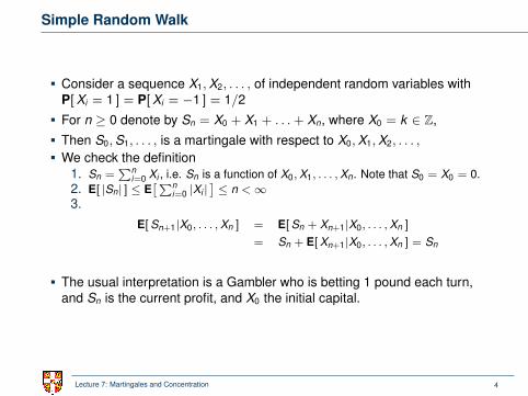
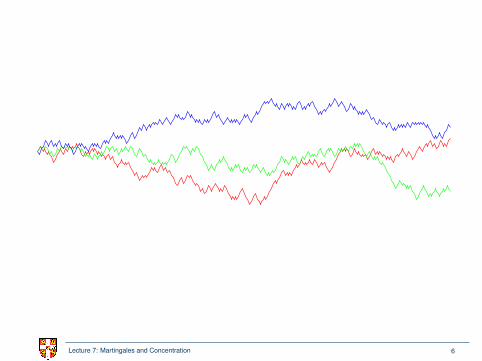
Simple Random Walk
Consider a sequence X1,X2, . . . , of independent random variables withP[Xi = 1 ] = P[Xi = −1 ] = 1/2
For n ≥ 0 denote by Sn = X0 + X1 + . . .+ Xn, where X0 = k ∈ Z,
Then S0,S1, . . . , is a martingale with respect to X0,X1,X2, . . . ,
We check the definition1. Sn =
∑ni=0 Xi , i.e. Sn is a function of X0,X1, . . . ,Xn. Note that S0 = X0 = 0.
2. E[ |Sn| ] ≤ E[∑n
i=0 |Xi |]≤ n <∞
3.
E[ Sn+1|X0, . . . ,Xn ] = E[ Sn + Xn+1|X0, . . . ,Xn ]
= Sn + E[ Xn+1|X0, . . . ,Xn ] = Sn
The usual interpretation is a Gambler who is betting 1 pound each turn,and Sn is the current profit, and X0 the initial capital.
Lecture 7: Martingales and Concentration 4
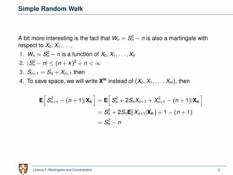
Simple Random Walk
A bit more interesting is the fact that Wn = S2n − n is also a martingale with
respect to X0,X1, . . . ,
1. Wn = S2n − n is a function of X0,X1, . . . ,Xn
2. |S2n − n| ≤ (n + k)2 + n <∞
3. Sn+1 = Sn + Xn+1 then
4. To save space, we will write Xm instead of (X0,X1, . . . ,Xm), then
E[
S2n+1 − (n + 1)|Xn
]= E
[S2
n + 2SnXn+1 + X 2n+1 − (n + 1)|Xn
]= S2
n + 2SnE[Xn+1|Xn ] + 1− (n + 1)
= S2n − n
Lecture 7: Martingales and Concentration 5
Lecture 7: Martingales and Concentration 6
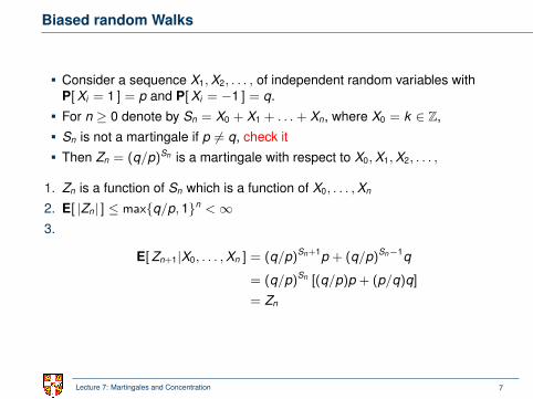
Biased random Walks
Consider a sequence X1,X2, . . . , of independent random variables withP[Xi = 1 ] = p and P[Xi = −1 ] = q.
For n ≥ 0 denote by Sn = X0 + X1 + . . .+ Xn, where X0 = k ∈ Z,
Sn is not a martingale if p 6= q, check it
Then Zn = (q/p)Sn is a martingale with respect to X0,X1,X2, . . . ,
1. Zn is a function of Sn which is a function of X0, . . . ,Xn
2. E[ |Zn| ] ≤ maxq/p, 1n <∞3.
E[Zn+1|X0, . . . ,Xn ] = (q/p)Sn+1p + (q/p)Sn−1q
= (q/p)Sn [(q/p)p + (p/q)q]
= Zn
Lecture 7: Martingales and Concentration 7
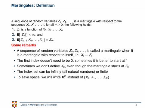
Martingales: Definition
A sequence of random variables Z0,Z1, . . . , is a martingale with respect to thesequence X0,X1, . . . , if, for all n ≥ 0, the following holds:1. Zn is a function of X0,X1, . . . ,Xn
2. E[ |Zn| ] <∞, and
3. E[ Zn+1|X0, . . . ,Xn ] = Zn.
Some remarksA sequence of random variables Z0,Z1, . . . , is called a martingale when itis a martingale with respect to itself, i.e. Xi = Zi .
The first index doesn’t need to be 0, sometimes it is better to start at 1
Sometimes we don’t define X0, even though the martingale starts at Z0
The index set can be infinity (all natural numbers) or finite
To save space, we will write Xm instead of (X0,X1, . . . ,Xm)
This is very obnoxious
Lecture 7: Martingales and Concentration 8
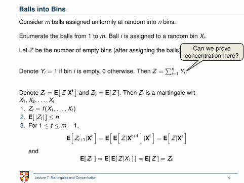
Balls into Bins
Consider m balls assigned uniformly at random into n bins.
Enumerate the balls from 1 to m. Ball i is assigned to a random bin Xi .
Let Z be the number of empty bins (after assigning the balls)
Denote Yi = 1 if bin i is empty, 0 otherwise. Then Z =∑n
i=1 Yi .
Can we proveconcentration here?
Denote Zt = E[
Z |Xt ] and Z0 = E[Z ]. Then Zt is a martingale wrtX1,X2, . . . ,Xt
1. Zt = f (X1, . . . ,Xt)
2. E[ |Zt | ] ≤ n3. For 1 ≤ t ≤ m − 1,
E[
Zt+1|Xt]= E
[E[
Z |Xt+1]|Xt]= E
[Z |Xt
]and
E[Z1 ] = E[E[Z |X1 ] ] = E[Z ] = Z0
Lecture 7: Martingales and Concentration 9

Martingales: Doob Martingale
A Doob martingale refers to a generic construction that is always amartingale. The construction is as follows.
Let X0, . . . ,Xn be a sequence of random variables.
Let Y be another random variable with E[ |Y | ] <∞ (usually Y is afunction of X0, . . . ,Xn).
Define Zi = E[
Y |Xi ].Z0, . . . ,Zn is a martingale w.r.t X0, . . . ,Xn
1. Clearly Zi is a function of X0, . . . ,Xi .2. E[ |Zi | ] = E
[|E[
Y |Xi ] | ] ≤ E[
E[|Y ||Xi ] ] = E[ |Y | ] <∞.
3.E[
Zi+1
∣∣∣Xi]
= E[
E[
Y∣∣∣Xi+1
] ∣∣∣Xi]
= E[
Y∣∣∣Xi]
= Zi
In most applications, X0 is undefined/ignored and Z0 corresponds to E[Y ]while Zn = Y .
Lecture 7: Martingales and Concentration 10
Example of Doob Martingale: Edge Exposure Martingale
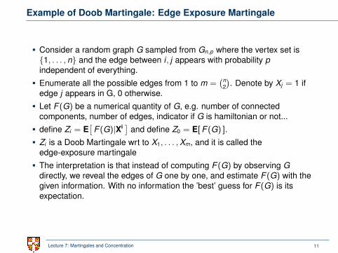
Consider a random graph G sampled from Gn,p where the vertex set is1, . . . , n and the edge between i, j appears with probability pindependent of everything.
Enumerate all the possible edges from 1 to m =(n
2
). Denote by Xj = 1 if
edge j appears in G, 0 otherwise.
Let F (G) be a numerical quantity of G, e.g. number of connectedcomponents, number of edges, indicator if G is hamiltonian or not...
define Zi = E[
F (G)|Xi ] and define Z0 = E[F (G) ].
Zi is a Doob Martingale wrt to X1, . . . ,Xm, and it is called theedge-exposure martingale
The interpretation is that instead of computing F (G) by observing Gdirectly, we reveal the edges of G one by one, and estimate F (G) with thegiven information. With no information the ’best’ guess for F (G) is itsexpectation.
Lecture 7: Martingales and Concentration 11
Example of Doob Martingale: Vertex Exposure Martingale
Similarly, instead of reveal edges one at a time, we can reveal vertices(with the corresponding edges), one at a time.
Fix the vertices from 1 to n, and let Gi be the subgraph of G induced bythe first i vertices.
let Z0 = E[F (G) ] and Zi = E[F (G)|G1, . . . ,Gi ]
this Doob martingale is called the vertex-exposure martingale
Lecture 7: Martingales and Concentration 12

Outline
Martingales
Martingale Concentration Inequalities
Examples
Lecture 7: Martingales and Concentration 13
Martingales: Azuma-Hoeffding Inequality
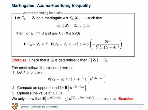
Let Z0, . . .Zn be a martingale wrt X0,X1, . . . , such that
ak ≤ Zk − Zk−1 ≤ bk
Then, for all t ≥ 0 and any k > 0 it holds
P[Zk − Z0 ≥ t ] ,P[Zk − Z0 ≤ −t ] ≤ exp
(− 2t2∑k
i=1(bi − ai)2
)
Azuma-Hoeffding Inequality
Exercise. Check that if Z0 is deterministic then E[Zk ] = Z0.
The proof follows the standard recipe.1. Let λ > 0, then
P[Zk − Z0 ≥ t ] ≤ e−λtE[
eλ(Zk−Z0)]
2. Compute an upper bound for E[
eλ(Zk−Z0)]
3. Optimise the value of λ > 0.We only show that E
[eλ(Zk−Z0)
]≤ e
∑ki=1 λ
2(bi−ai )2/8, the rest is an Exercise.
Lecture 7: Martingales and Concentration 14
Martingales: Azuma-Hoeffding Inequality
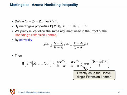
Define Yi = Zi − Zi−1 for i ≥ 1.
By martingale properties E[Yi |X0,X1, . . . ,Xi−1 ] = 0.
We pretty much follow the same argument used in the Proof of theHoeffding’s Extension Lemma
By convexity
eλYi ≤ bi − Yi
bi − aieλai +
Yi − ai
bi − aieλbi
Then
E[
eλYi∣∣∣X0, . . . ,Xi−1
]≤ bieλai
bi − ai− aieλbi
bi − ai≤ exp
[(bi − ai)
2λ2
8
]Exactly as in the Hoefd-ding’s Extension Lemma
Lecture 7: Martingales and Concentration 15
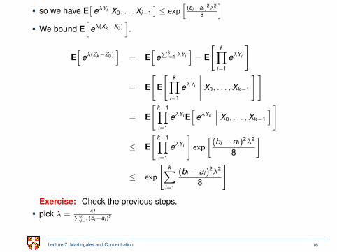
so we have E[
eλYi |X0, . . .Xi−1]≤ exp
[(bi−ai )
2λ2
8
]We bound E
[eλ(Xk−X0)
].
E[
eλ(Zk−Z0)]
= E[
e∑k
i=1 λYi]= E
[k∏
i=1
eλYi
]
= E
[E
[k∏
i=1
eλYi
∣∣∣∣∣ X0, . . . ,Xk−1
]]
= E
[k−1∏i=1
eλYi E[
eλYk∣∣∣ X0, . . . ,Xk−1
] ]
≤ E
[k−1∏i=1
eλYi
]exp
[(bi − ai)
2λ2
8
]
≤ exp
[k∑
i=1
(bi − ai)2λ2
8
]
Exercise: Check the previous steps.pick λ = 4t∑n
i=1(bi−ai )2
Lecture 7: Martingales and Concentration 16
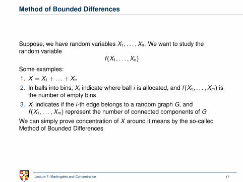
Method of Bounded Differences
Suppose, we have random variables X1, . . . ,Xn. We want to study therandom variable
f (X1, . . . ,Xn)
Some examples:
1. X = X1 + . . .+ Xn
2. In balls into bins, Xi indicate where ball i is allocated, and f (X1, . . . ,Xm) isthe number of empty bins
3. Xi indicates if the i-th edge belongs to a random graph G, andf (X1, . . . ,Xm) represent the number of connected components of G
We can simply prove concentration of X around it means by the so-calledMethod of Bounded Differences
Lecture 7: Martingales and Concentration 17
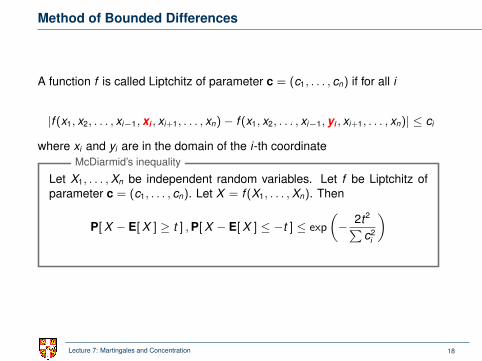
Method of Bounded Differences
A function f is called Liptchitz of parameter c = (c1, . . . , cn) if for all i
|f (x1, x2, . . . , xi−1, xi , xi+1, . . . , xn)− f (x1, x2, . . . , xi−1, yi , xi+1, . . . , xn)| ≤ ci
where xi and yi are in the domain of the i-th coordinate
Let X1, . . . ,Xn be independent random variables. Let f be Liptchitz ofparameter c = (c1, . . . , cn). Let X = f (X1, . . . ,Xn). Then
P[X − E[X ] ≥ t ] ,P[X − E[X ] ≤ −t ] ≤ exp
(− 2t2∑
c2i
)McDiarmid’s inequality
Lecture 7: Martingales and Concentration 18
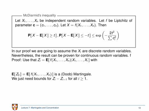
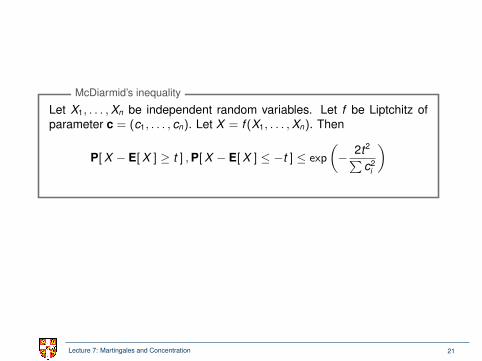
Let X1, . . . ,Xn be independent random variables. Let f be Liptchitz ofparameter c = (c1, . . . , cn). Let X = f (X1, . . . ,Xn). Then
P[X − E[X ] ≥ t ] ,P[X − E[X ] ≤ −t ] ≤ exp
(− 2t2∑
c2i
)McDiarmid’s inequality
In our proof we are going to assume the Xi are discrete random variables.Nevertheless, the result can be proven for continuous random variables. fProof: Use that Zi = E[ f (X1, . . . ,Xn)|X1, . . . ,Xi ] with
E[Z0 ] = E[ f (X1, . . . ,Xn) ] is a (Doob) Martingale.We just need bounds for Zi − Zi−1 for all i ≥ 1.
Lecture 7: Martingales and Concentration 19
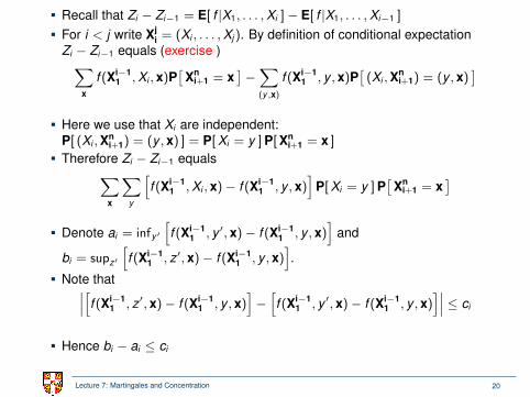
Recall that Zi − Zi−1 = E[ f |X1, . . . ,Xi ]− E[ f |X1, . . . ,Xi−1 ]
For i < j write Xji = (Xi , . . . ,Xj). By definition of conditional expectation
Zi − Zi−1 equals (exercise )∑x
f (Xi−11 ,Xi , x)P
[Xn
i+1 = x]−∑(y,x)
f (Xi−11 , y , x)P
[(Xi ,Xn
i+1) = (y , x)]
Here we use that Xi are independent:P[ (Xi ,Xn
i+1) = (y , x) ] = P[Xi = y ]P[Xni+1 = x ]
Therefore Zi − Zi−1 equals∑x
∑y
[f (Xi−1
1 ,Xi , x)− f (Xi−11 , y , x)
]P[Xi = y ]P
[Xn
i+1 = x]
Denote ai = infy′
[f (Xi−1
1 , y ′, x)− f (Xi−11 , y , x)
]and
bi = supz′
[f (Xi−1
1 , z′, x)− f (Xi−11 , y , x)
].
Note that∣∣∣[f (Xi−11 , z′, x)− f (Xi−1
1 , y , x)]−[f (Xi−1
1 , y ′, x)− f (Xi−11 , y , x)
]∣∣∣ ≤ ci
Hence bi − ai ≤ ci
Lecture 7: Martingales and Concentration 20
Let X1, . . . ,Xn be independent random variables. Let f be Liptchitz ofparameter c = (c1, . . . , cn). Let X = f (X1, . . . ,Xn). Then
P[X − E[X ] ≥ t ] ,P[X − E[X ] ≤ −t ] ≤ exp
(− 2t2∑
c2i
)McDiarmid’s inequality
Lecture 7: Martingales and Concentration 21

Outline
Martingales
Martingale Concentration Inequalities
Examples
Lecture 7: Martingales and Concentration 22
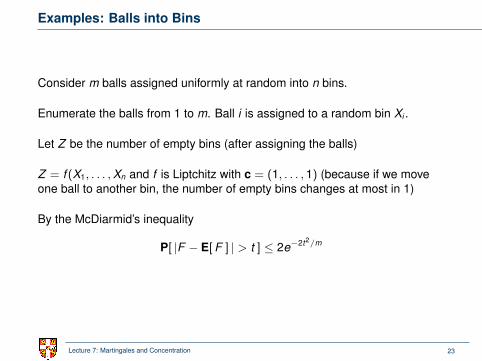
Examples: Balls into Bins
Consider m balls assigned uniformly at random into n bins.
Enumerate the balls from 1 to m. Ball i is assigned to a random bin Xi .
Let Z be the number of empty bins (after assigning the balls)
Z = f (X1, . . . ,Xn and f is Liptchitz with c = (1, . . . , 1) (because if we moveone ball to another bin, the number of empty bins changes at most in 1)
By the McDiarmid’s inequality
P[ |F − E[F ] | > t ] ≤ 2e−2t2/m
Lecture 7: Martingales and Concentration 23
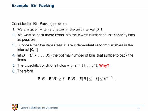
Example: Bin Packing
Consider the Bin Packing problem
1. We are given n items of sizes in the unit interval [0, 1]
2. We want to pack those items into the fewest number of unit-capacity binsas possible
3. Suppose that the item sizes Xi are independent random variables in theinterval [0, 1]
4. let B = B(X1, . . . ,Xn) the optimal number of bins that suffice to pack theitems
5. The Lipschitz conditions holds with c = (1, . . . , 1), Why?6. Therefore
P[B − E[B ] ≥ t ] ,P[B − E[B ] ≤ −t ] ≤ e−2t2/n.
Lecture 7: Martingales and Concentration 24
A random distance problem
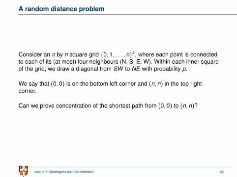
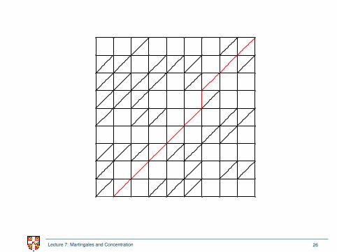
Consider an n by n square grid 0, 1, . . . , n2, where each point is connectedto each of its (at most) four neighbours (N, S, E, W). Within each inner squareof the grid, we draw a diagonal from SW to NE with probability p.
We say that (0, 0) is on the bottom left corner and (n, n) in the top rightcorner.
Can we prove concentration of the shortest path from (0, 0) to (n, n)?
Lecture 7: Martingales and Concentration 25
Lecture 7: Martingales and Concentration 26
A random distance problem
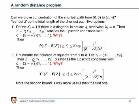
Can we prove concentration of the shortest path from (0, 0) to (n, n)?Yes! Let Z be the total length of the shortest path.Two options
1. Define Xij = 1 if there is a diagonal in square ij , otherwise Xij = 0. ThenZ = f (X11, . . . ,Xnn) satisfies the Lipschitz conditions withc = (2−
√2)(1, . . . , 1), Why? .
Then
P[ |Z − E[Z ] | ≥ t ] ≤ 2 exp
[−t2
(2−√
2)2n2
]2. Enumerate the columns of squares from 1 to n. Let Yi = (X1i , . . . ,Xni).
Then Z = g(Y1, . . . ,Yn). g satisfies the Lipschitz conditions withc = (2−
√2)(1, . . . , 1). Why?
Then
P[ |Z − E[Z ] | ≥ t ] ≤ 2 exp
[−t2
(2−√
2)2n
]Note the second bound is way more useful than the first one.
Lecture 7: Martingales and Concentration 27
Example: Clique Number in Random Graphs
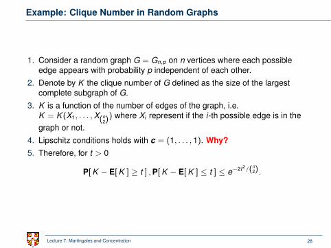
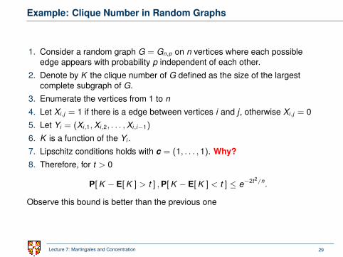
1. Consider a random graph G = Gn,p on n vertices where each possibleedge appears with probability p independent of each other.
2. Denote by K the clique number of G defined as the size of the largestcomplete subgraph of G.
3. K is a function of the number of edges of the graph, i.e.K = K (X1, . . . ,X(n
2)) where Xi represent if the i-th possible edge is in the
graph or not.
4. Lipschitz conditions holds with c = (1, . . . , 1). Why?5. Therefore, for t > 0
P[K − E[K ] ≥ t ] ,P[K − E[K ] ≤ t ] ≤ e−2t2/(n2).
Lecture 7: Martingales and Concentration 28
Example: Clique Number in Random Graphs
1. Consider a random graph G = Gn,p on n vertices where each possibleedge appears with probability p independent of each other.
2. Denote by K the clique number of G defined as the size of the largestcomplete subgraph of G.
3. Enumerate the vertices from 1 to n
4. Let Xi,j = 1 if there is a edge between vertices i and j , otherwise Xi,j = 0
5. Let Yi = (Xi,1,Xi,2, . . . ,Xi,i−1)
6. K is a function of the Yi .
7. Lipschitz conditions holds with c = (1, . . . , 1). Why?8. Therefore, for t > 0
P[K − E[K ] > t ] ,P[K − E[K ] < t ] ≤ e−2t2/n.
Observe this bound is better than the previous one
Lecture 7: Martingales and Concentration 29
MaxCut on Random Graphs
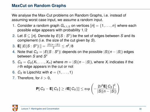
We analyse the Max-Cut problems on Random Graphs, i.e. instead ofassuming worst case input, we assume a random input.
1. Consider a random graph Gn,1/2 on vertices [n] = 1, . . . , n where eachpossible edge appears with probability 1/2
2. Let S ⊆ [n]. Denote by E(S : Sc) be the set of edges between S and itscomplement (i.e. the size of the cut given by S).
3. E[ |E(S : Sc)| ] = |S|(n−|S|)2 ≤ n2/8
4. Note that CS = |E(S : Sc)| depends on the possible |S|(n − |S|) edgesbetween S and Sc
5. CS = CS(X1, . . . ,Xm) where m = |S|(n − |S|), where Xi indicates if thei-th edge appears in the cut or not
6. CS is Lipschitz with c = (1, . . . , 1)
7. Therefore, for δ > 0,
P[CS − E[CS ] ≥ δE[CS ] ] ≤ exp
(− 2δ2E[CS ]2
|S|(n − |S|)
)
Lecture 7: Martingales and Concentration 30

8. Exercise: Deduce that for any S ⊆ [n],
P[
CS ≥n2
8+ δ
n2
4
]≤ e−Ω(δ2n2)
9. By the union bound, we have that
P[∃S : CS ≥
n2
8+ δ
n2
4
]≤ 2ne−Ω(δ2n2) = 2ne−Ω(c2n)
10. Recall that δ = c/√
n, now we pick c to be large enough, such that2ne−Ω(c2n) = 2−n
11. The main result is:
There is a constant c, such that w.h.p. the Max Cut in Gn,1/2 is at mostn2/8 + cn1/2
Theorem
Lecture 7: Martingales and Concentration 31


![LE MARTINGALE: ASPETTI TEORICI ED APPLICATIVI The ...Ceris-Cnr, W.P. N 7/2001 LE MARTINGALE: ASPETTI TEORICI ED APPLICATIVI [The martingales: theoretical and empirical characteristics]Fabrizio](https://img.pdfslide.net/doc/110x75/60ce46ea67ed16281b38b2ce/le-martingale-aspetti-teorici-ed-applicativi-the-ceris-cnr-wp-n-72001-le.jpg)