Lecture 9: Decision TreeShuai Li

John Hopcroft Center, Shanghai Jiao Tong University

https://shuaili8.github.io

https://shuaili8.github.io/Teaching/VE445/index.html

1

Outline

• Tree models

• Information theory• Entropy, cross entropy, information gain

• Decision tree

• Continuous labels• Standard deviation

2

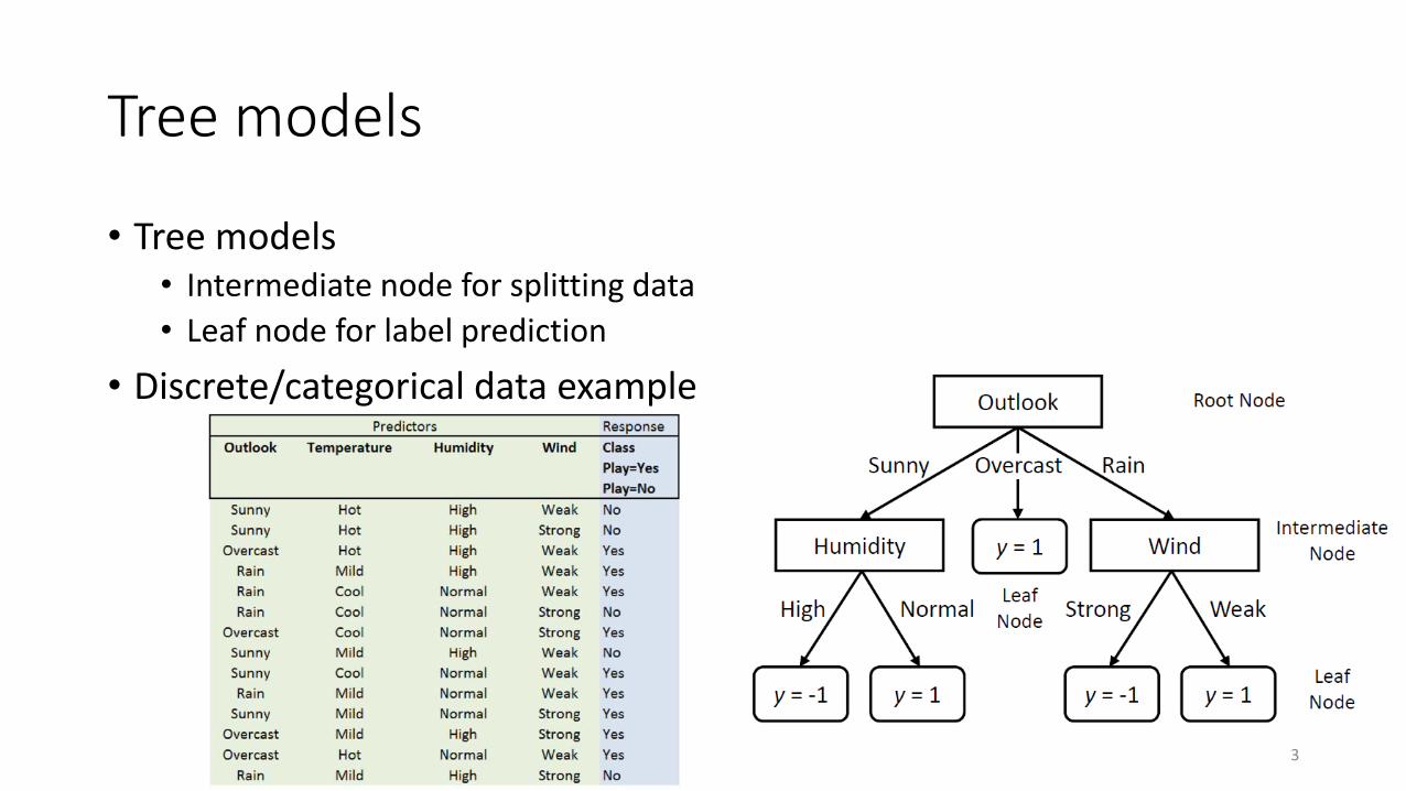
Tree models

• Tree models• Intermediate node for splitting data

• Leaf node for label prediction

• Discrete/categorical data example

3

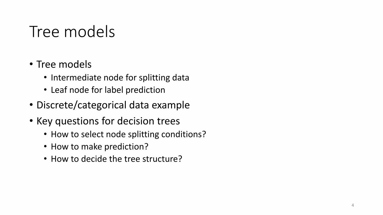
Tree models

• Tree models• Intermediate node for splitting data

• Leaf node for label prediction

• Discrete/categorical data example

• Key questions for decision trees• How to select node splitting conditions?

• How to make prediction?

• How to decide the tree structure?

4

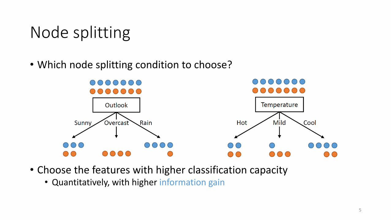
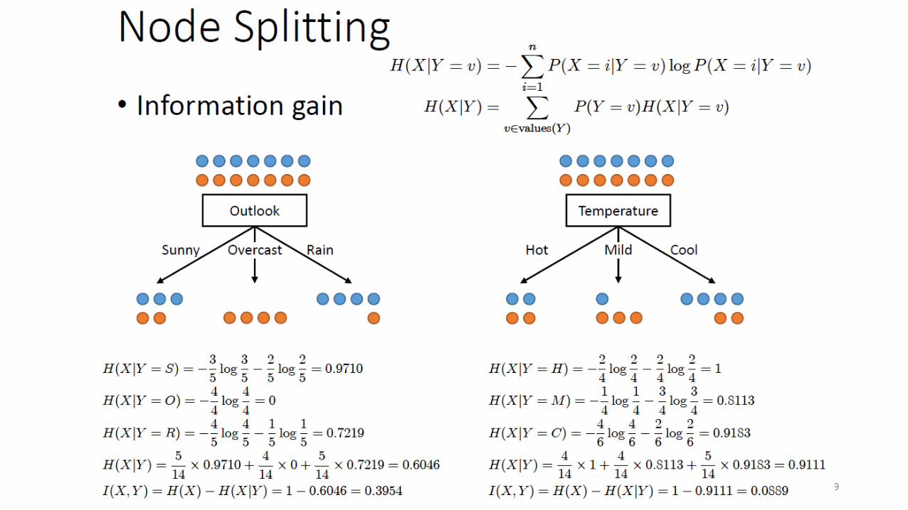
Node splitting

• Which node splitting condition to choose?

• Choose the features with higher classification capacity• Quantitatively, with higher information gain

5

Information Theory

6

Motivating example 1

• Suppose you are a police officer and there was a robbery last night. There are several suspects and you want to find the criminal from them by asking some questions.

• You may ask: where are you last night?

• You are not likely to ask: what is your favorite food?

• Why there is a preference for the policeman? Because the first one can distinguish the guilty from the innocent. It is more informative.

7

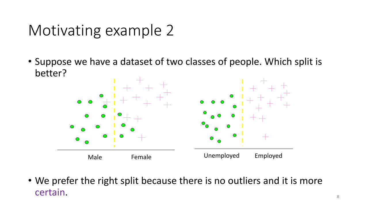
Motivating example 2

• Suppose we have a dataset of two classes of people. Which split is better?

• We prefer the right split because there is no outliers and it is more certain.

8

FemaleMale EmployedUnemployed

Entropy

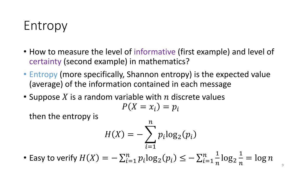
• How to measure the level of informative (first example) and level of certainty (second example) in mathematics?

• Entropy (more specifically, Shannon entropy) is the expected value (average) of the information contained in each message

• Suppose 𝑋 is a random variable with 𝑛 discrete values𝑃 𝑋 = 𝑥𝑖 = 𝑝𝑖

then the entropy is

𝐻 𝑋 = −

𝑖=1

𝑛

𝑝𝑖log2 𝑝𝑖

• Easy to verify 𝐻 𝑋 = −σ𝑖=1𝑛 𝑝𝑖log2 𝑝𝑖 ≤ −σ𝑖=1

𝑛 1

𝑛log2

1

𝑛= log 𝑛

9

Illustration

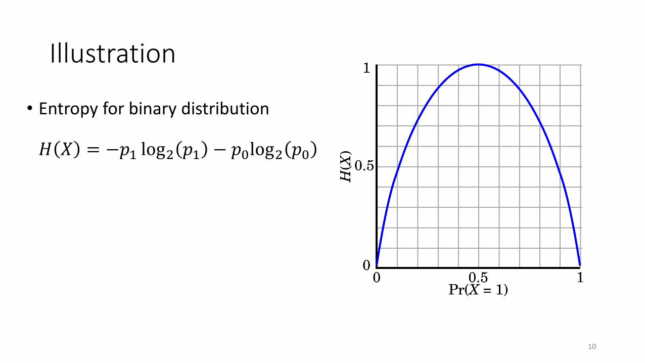
• Entropy for binary distribution

𝐻 𝑋 = −𝑝1 log2 𝑝1 − 𝑝0log2 𝑝0

10

Entropy examples

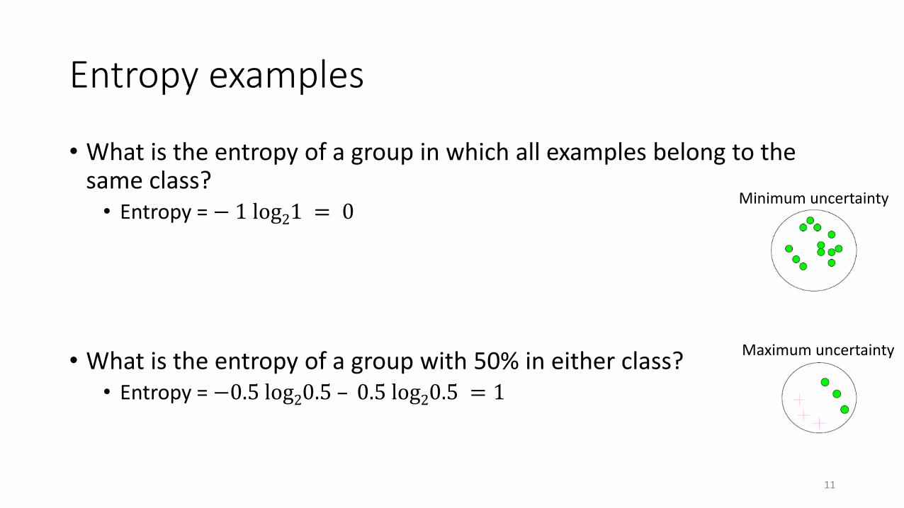
• What is the entropy of a group in which all examples belong to the same class?• Entropy = − 1 log21 = 0

• What is the entropy of a group with 50% in either class?• Entropy = −0.5 log20.5 – 0.5 log20.5 = 1

11

Minimum uncertainty

Maximum uncertainty

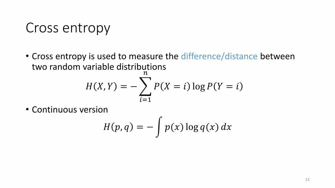
Cross entropy

• Cross entropy is used to measure the difference/distance between two random variable distributions

𝐻 𝑋, 𝑌 = −

𝑖=1

𝑛

𝑃 𝑋 = 𝑖 log 𝑃 𝑌 = 𝑖

• Continuous version

𝐻 𝑝, 𝑞 = −න𝑝(𝑥) log 𝑞(𝑥) 𝑑𝑥

12

Recall on logistic regression

• Binary classification

• Cross entropy loss function

• Gradient

is also convex in 𝜃

13

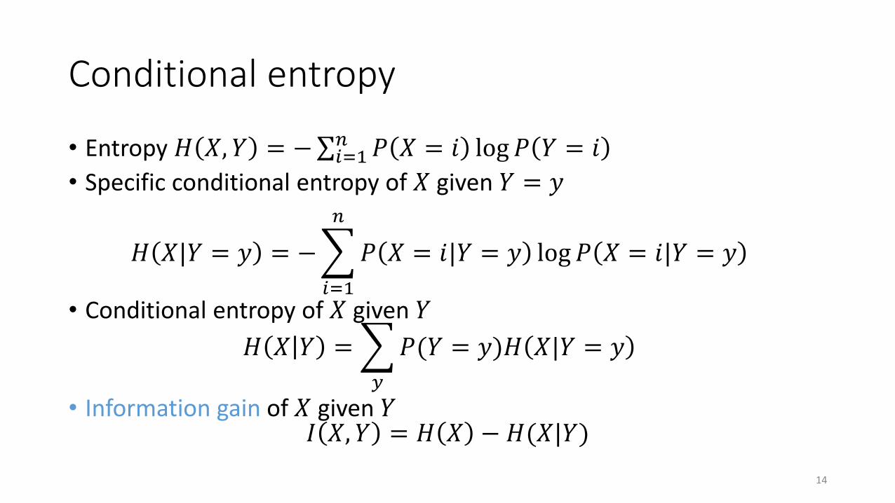
Conditional entropy

• Entropy 𝐻 𝑋, 𝑌 = −σ𝑖=1𝑛 𝑃 𝑋 = 𝑖 log 𝑃 𝑌 = 𝑖

• Specific conditional entropy of 𝑋 given 𝑌 = 𝑦

𝐻 𝑋|𝑌 = 𝑦 = −

𝑖=1

𝑛

𝑃 𝑋 = 𝑖|𝑌 = 𝑦 log 𝑃 𝑋 = 𝑖|𝑌 = 𝑦

• Conditional entropy of 𝑋 given 𝑌

𝐻 𝑋 𝑌 =

𝑦

𝑃(𝑌 = 𝑦)𝐻 𝑋|𝑌 = 𝑦

• Information gain of 𝑋 given 𝑌𝐼 𝑋, 𝑌 = 𝐻 𝑋 − 𝐻(𝑋|𝑌)

14

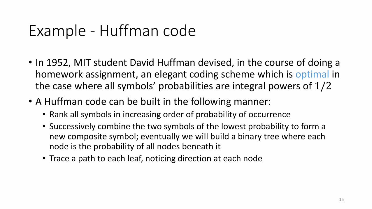
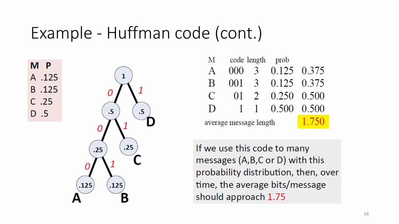
Example - Huffman code

• In 1952, MIT student David Huffman devised, in the course of doing a homework assignment, an elegant coding scheme which is optimal in the case where all symbols’ probabilities are integral powers of 1/2

• A Huffman code can be built in the following manner:• Rank all symbols in increasing order of probability of occurrence

• Successively combine the two symbols of the lowest probability to form a new composite symbol; eventually we will build a binary tree where each node is the probability of all nodes beneath it

• Trace a path to each leaf, noticing direction at each node

15

Example - Huffman code (cont.)

16

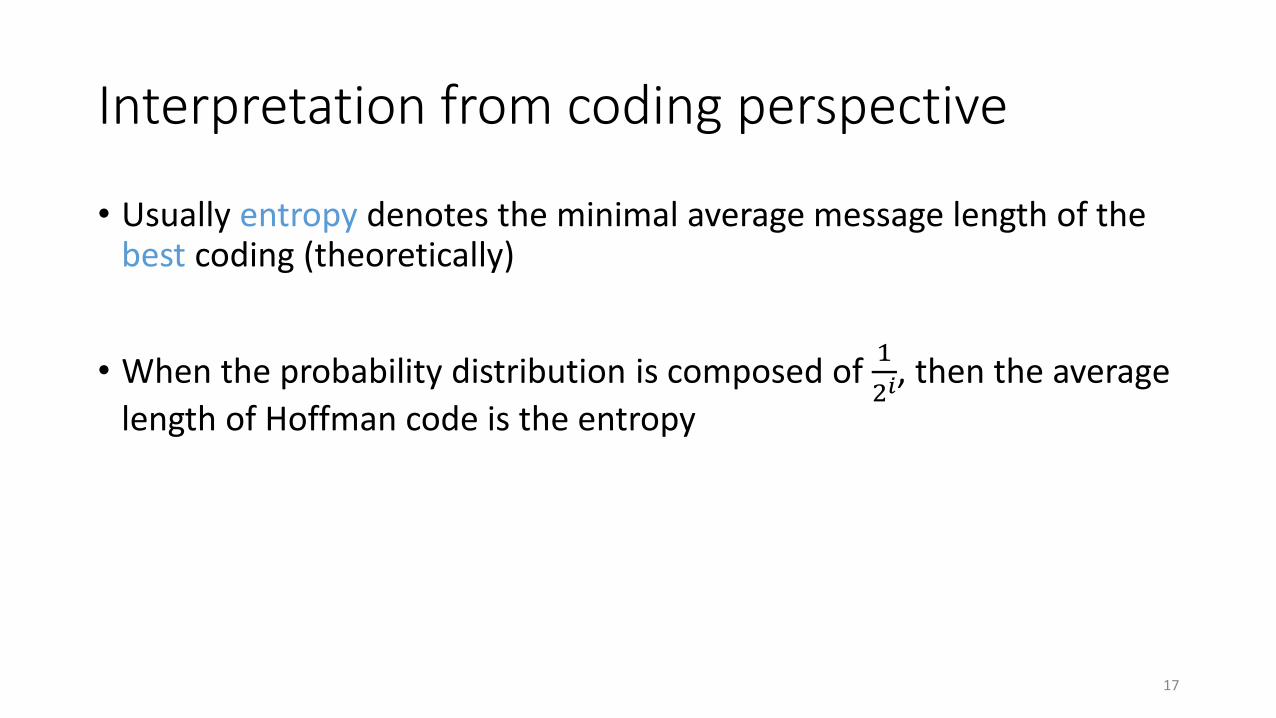
Interpretation from coding perspective

• Usually entropy denotes the minimal average message length of the best coding (theoretically)

• When the probability distribution is composed of 1

2𝑖, then the average

length of Hoffman code is the entropy

17

Decision Tree

18

19

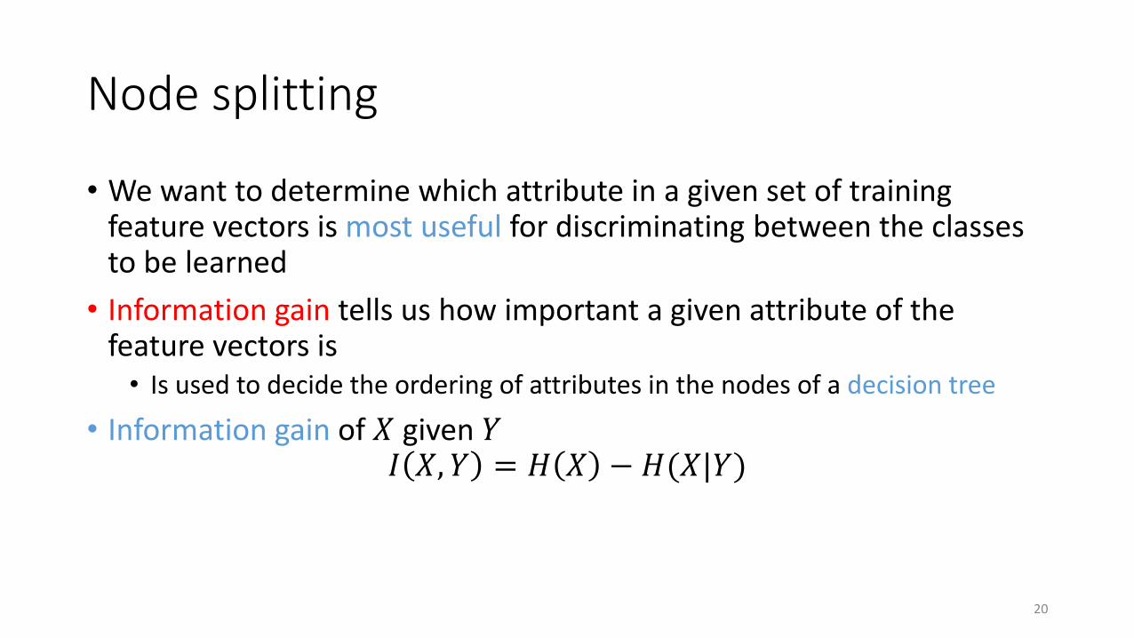
Node splitting

• We want to determine which attribute in a given set of training feature vectors is most useful for discriminating between the classes to be learned

• Information gain tells us how important a given attribute of the feature vectors is• Is used to decide the ordering of attributes in the nodes of a decision tree

• Information gain of 𝑋 given 𝑌𝐼 𝑋, 𝑌 = 𝐻 𝑋 − 𝐻(𝑋|𝑌)

20

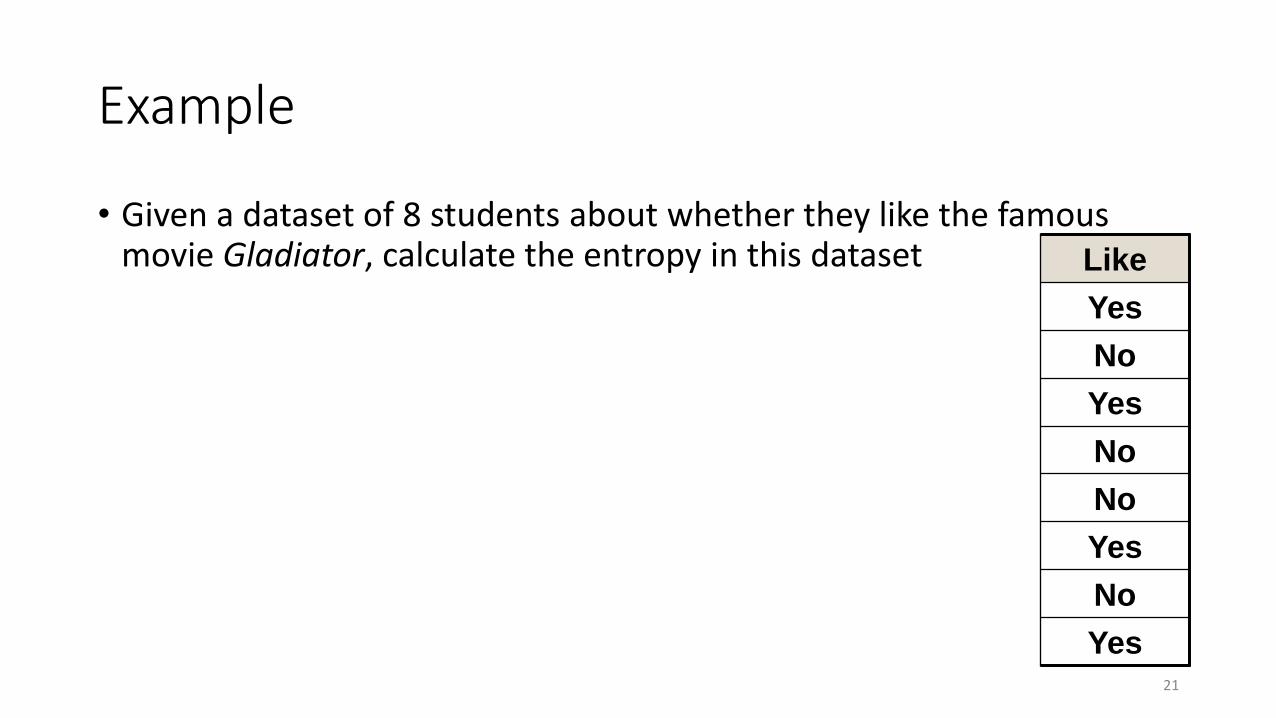
Example

• Given a dataset of 8 students about whether they like the famous movie Gladiator, calculate the entropy in this dataset

21

Like

Yes

No

Yes

No

No

Yes

No

Yes

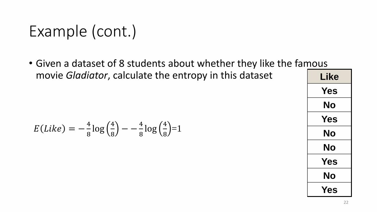
Example (cont.)

• Given a dataset of 8 students about whether they like the famous movie Gladiator, calculate the entropy in this dataset

22

𝐸 𝐿𝑖𝑘𝑒 = −4

8log

4

8−−

4

8log

4

8=1

Like

Yes

No

Yes

No

No

Yes

No

Yes

Example (cont.)

• Suppose we now also know the gender of these 8 students, what is the conditional entropy on gender?

23

Gender Like

Male Yes

Female No

Male Yes

Female No

Female No

Male Yes

Male No

Female Yes

Example (cont.)

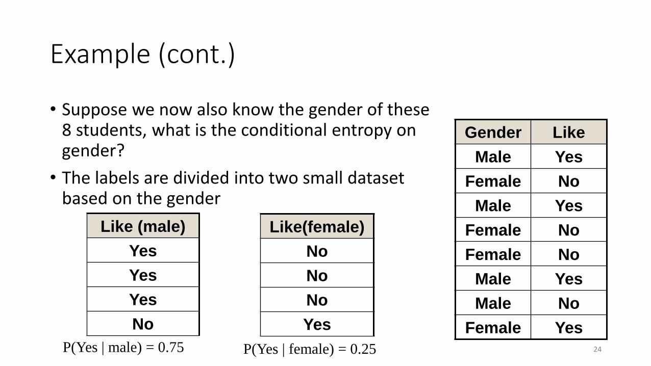
• Suppose we now also know the gender of these 8 students, what is the conditional entropy on gender?

• The labels are divided into two small dataset based on the gender

24P(Yes | male) = 0.75 P(Yes | female) = 0.25

Gender Like

Male Yes

Female No

Male Yes

Female No

Female No

Male Yes

Male No

Female Yes

Like (male)

Yes

Yes

Yes

No

Like(female)

No

No

No

Yes

Example (cont.)

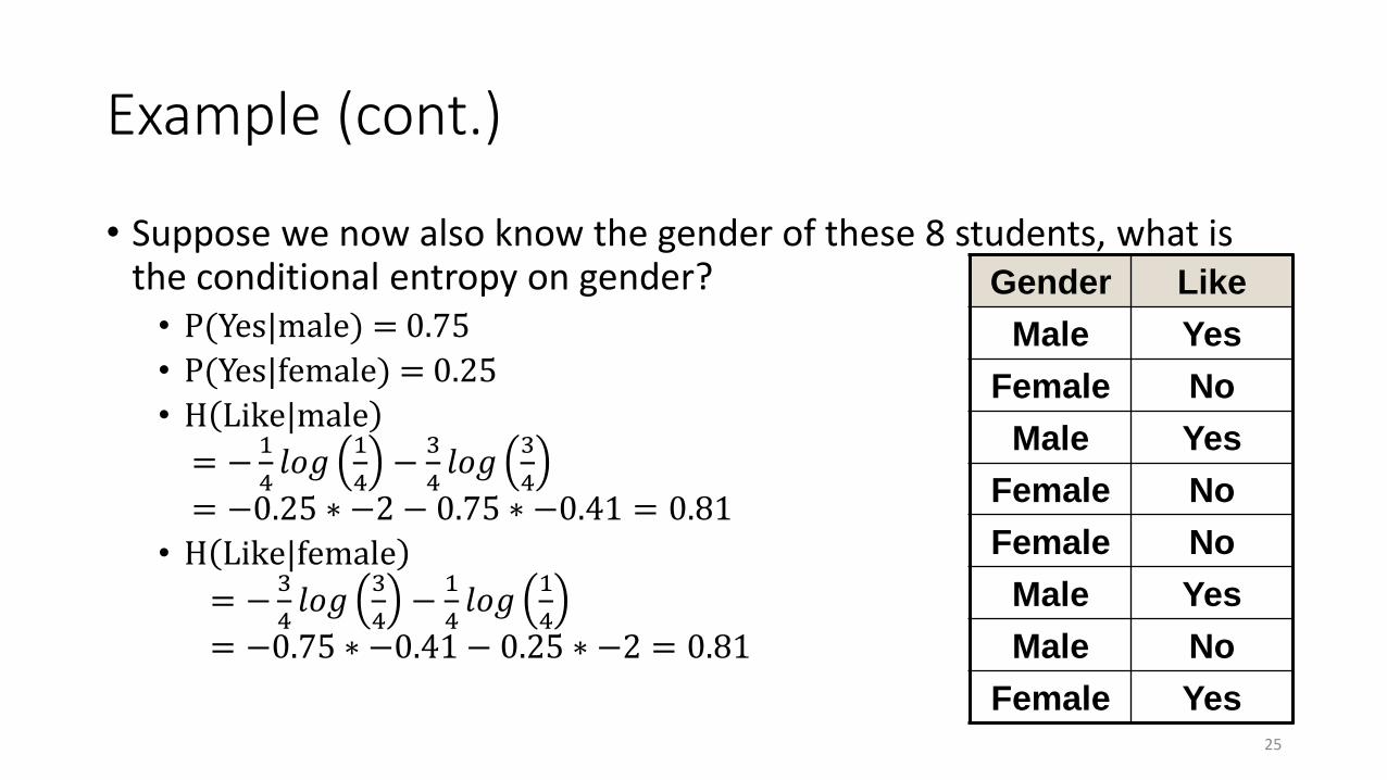
• Suppose we now also know the gender of these 8 students, what is the conditional entropy on gender?• P(Yes|male) = 0.75

• P(Yes|female) = 0.25

• H Like|male

= −1

4𝑙𝑜𝑔

1

4−

3

4𝑙𝑜𝑔

3

4= −0.25 ∗ −2 − 0.75 ∗ −0.41 = 0.81

• H Like|female

= −3

4𝑙𝑜𝑔

3

4−

1

4𝑙𝑜𝑔

1

4= −0.75 ∗ −0.41 − 0.25 ∗ −2 = 0.81

25

Gender Like

Male Yes

Female No

Male Yes

Female No

Female No

Male Yes

Male No

Female Yes

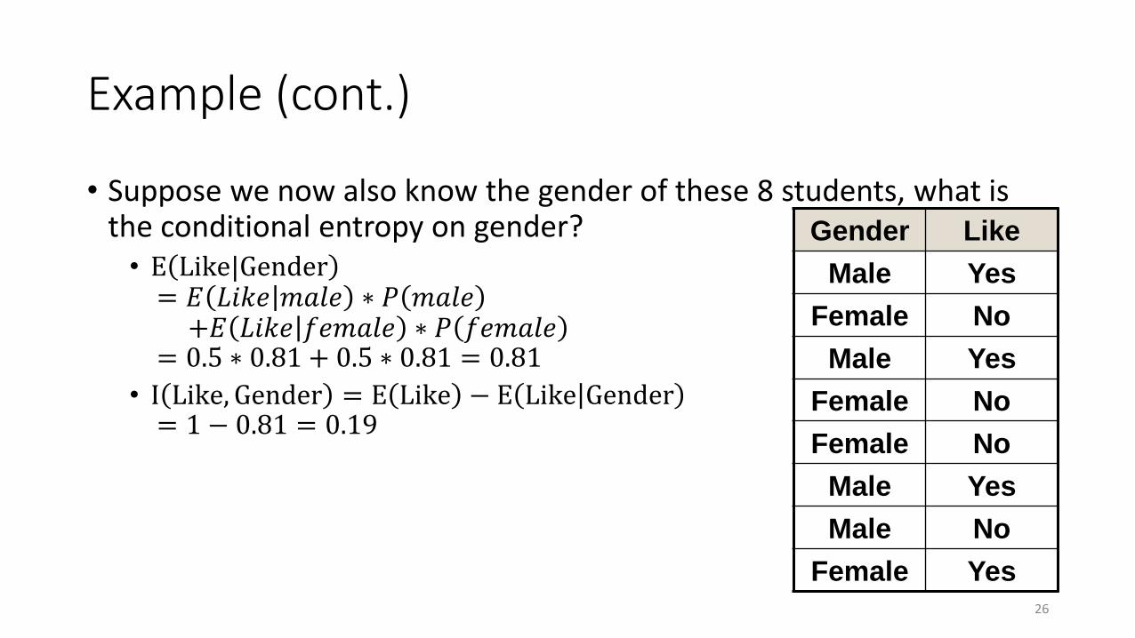
Example (cont.)

• Suppose we now also know the gender of these 8 students, what is the conditional entropy on gender?• E Like|Gender= 𝐸 𝐿𝑖𝑘𝑒 𝑚𝑎𝑙𝑒 ∗ 𝑃 𝑚𝑎𝑙𝑒+𝐸 𝐿𝑖𝑘𝑒 𝑓𝑒𝑚𝑎𝑙𝑒 ∗ 𝑃 𝑓𝑒𝑚𝑎𝑙𝑒

= 0.5 ∗ 0.81 + 0.5 ∗ 0.81 = 0.81

• I Like, Gender = E Like − E Like Gender= 1 − 0.81 = 0.19

26

Gender Like

Male Yes

Female No

Male Yes

Female No

Female No

Male Yes

Male No

Female Yes

Example (cont.)

• Suppose we now also know the major of these 8 students, what about the conditional entropy on major?

27

Major Like

Math Yes

History No

CS Yes

Math No

Math No

CS Yes

History No

Math Yes

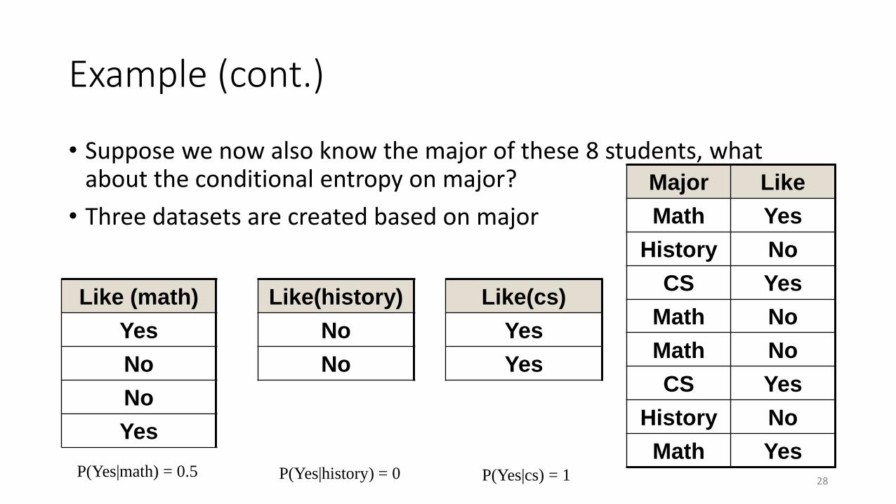
Example (cont.)

• Suppose we now also know the major of these 8 students, what about the conditional entropy on major?

• Three datasets are created based on major

28

Major Like

Math Yes

History No

CS Yes

Math No

Math No

CS Yes

History No

Math YesP(Yes|history) = 0 P(Yes|cs) = 1P(Yes|math) = 0.5

Like (math)

Yes

No

No

Yes

Like(history)

No

No

Like(cs)

Yes

Yes

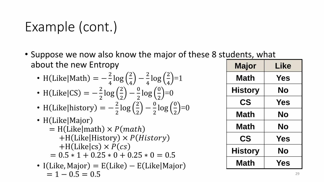
Example (cont.)

• Suppose we now also know the major of these 8 students, what about the new Entropy

• H Like|Math = −2

4log

2

4−

2

4log

2

4=1

• H Like|CS = −2

2log

2

2−

0

2log

0

2=0

• H Like|history = −2

2log

2

2−

0

2log

0

2=0

• H Like|Major= H Like math × 𝑃 𝑚𝑎𝑡ℎ

+H Like History × 𝑃 𝐻𝑖𝑠𝑡𝑜𝑟𝑦+H Like cs × 𝑃 𝑐𝑠

= 0.5 ∗ 1 + 0.25 ∗ 0 + 0.25 ∗ 0 = 0.5

• I Like,Major = E Like − E Like Major= 1 − 0.5 = 0.5 29

Major Like

Math Yes

History No

CS Yes

Math No

Math No

CS Yes

History No

Math Yes

Example (cont.)

• Compare gender and major

• As we have computed• I(Like, Gender) = E Like −E Like Gender = 1 − 0.81 = 0.19

• I(Like,Major) = E Like −E Like Major = 1 − 0.5 = 0.5

• Major is the better feature to predict the label “like”

30

Gender Major Like

Male Math Yes

Female History No

Male CS Yes

Female Math No

Female Math No

Male CS Yes

Male History No

Female Math Yes

Example (cont.)

• Major is used as the decision condition and it splits the dataset into three small one based on the answer

31

Gender Like

Male Yes

Female No

Female No

Female Yes

Gender Like

Female No

Male No

Major?

Math CS

Gender Like

Male Yes

Female Yes

History

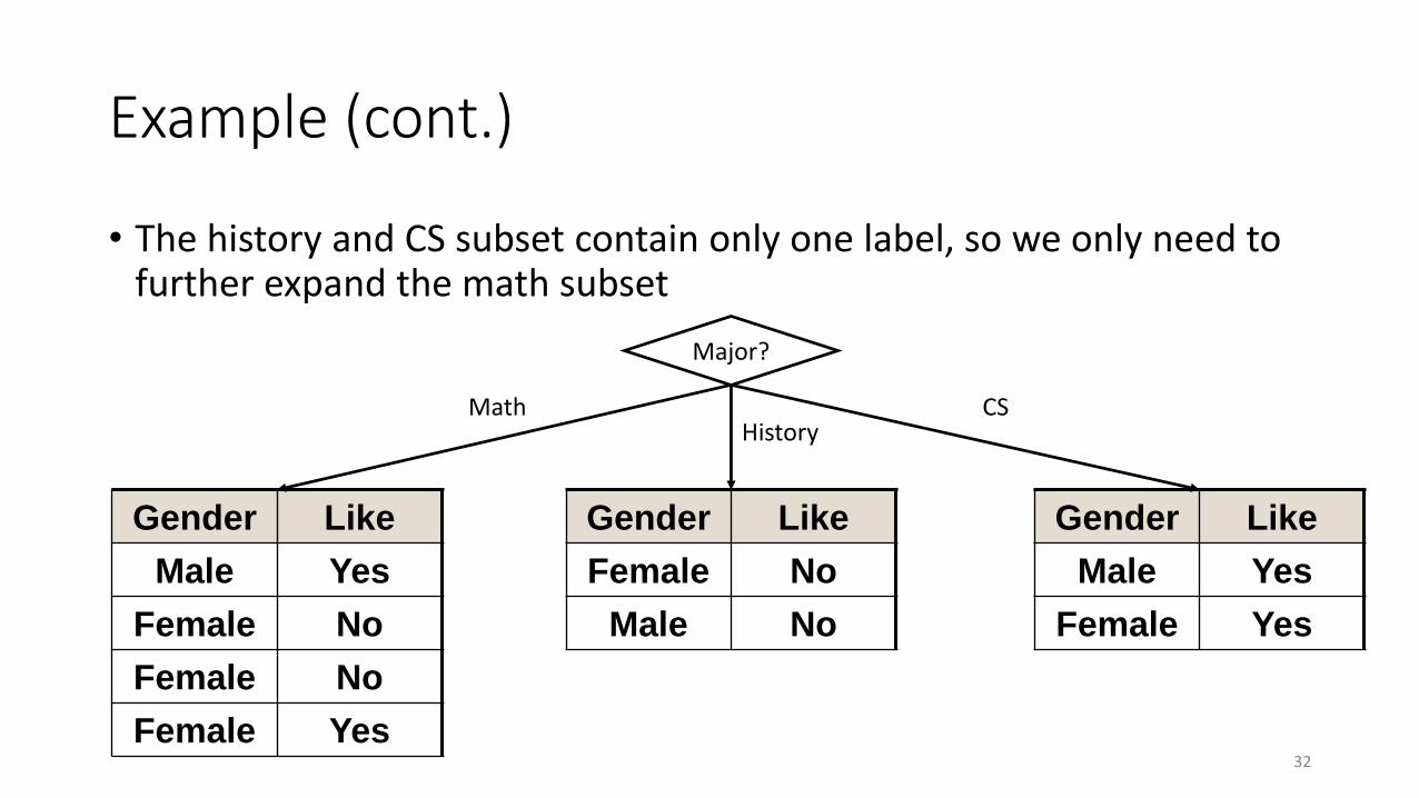
Example (cont.)

• The history and CS subset contain only one label, so we only need to further expand the math subset

32

Gender Like

Male Yes

Female No

Female No

Female Yes

Gender Like

Female No

Male No

Major?

Math CS

Gender Like

Male Yes

Female Yes

History

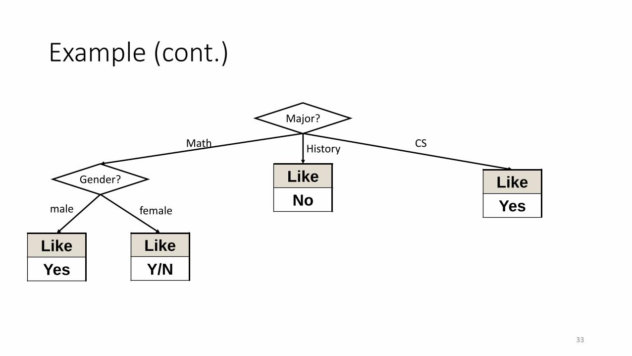
Example (cont.)

33

Major?

Math CSHistory

Like

Yes

Like

No

Gender?

female

Like

Y/N

Like

Yes

male

Example (cont.)

• In the stage of testing, suppose there come a female students from the CS department, how can we predict whether she like the movie Gladiator?• Based on the major of CS, we will directly predict she like the movie.

• What about a male student and a female student from math department?

34

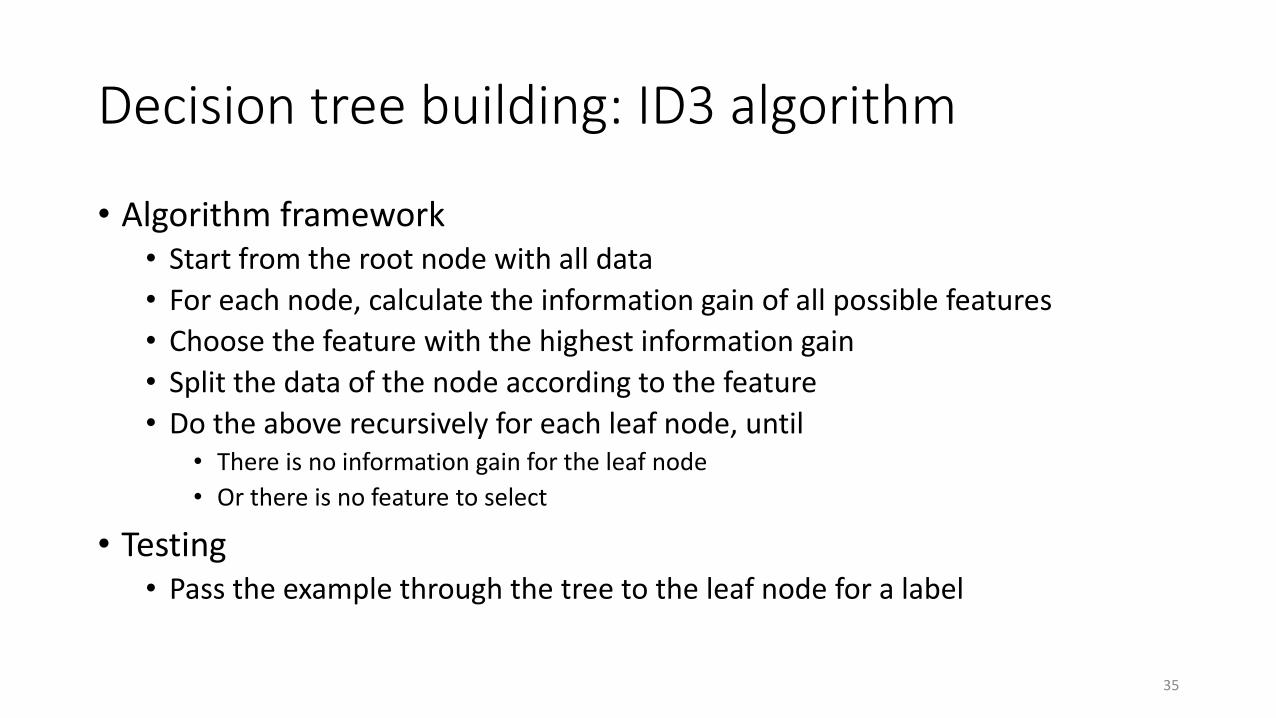
Decision tree building: ID3 algorithm

• Algorithm framework• Start from the root node with all data

• For each node, calculate the information gain of all possible features

• Choose the feature with the highest information gain

• Split the data of the node according to the feature

• Do the above recursively for each leaf node, until• There is no information gain for the leaf node

• Or there is no feature to select

• Testing• Pass the example through the tree to the leaf node for a label

35

Continuous Labels

36

Continuous label (regression)

• Previously, we have learned how to build a tree for classification, in which the labels are categorical values

• The mathematical tool to build a classification tree is entropy in information theory, which can only be applied in categorical labels

• To build a decision tree for regression (in which the labels are continuous values), we need new mathematical tools

37

Regression tree vs Classification tree

38

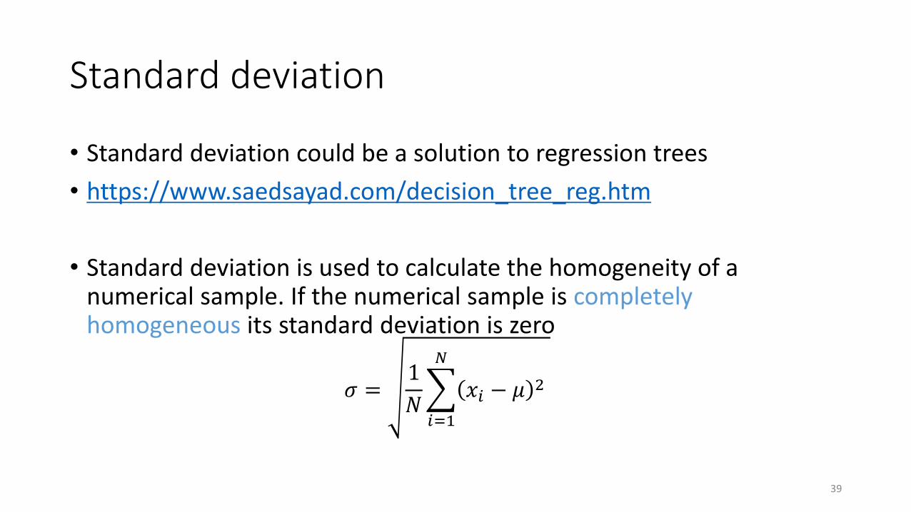
Standard deviation

• Standard deviation could be a solution to regression trees

• https://www.saedsayad.com/decision_tree_reg.htm

• Standard deviation is used to calculate the homogeneity of a numerical sample. If the numerical sample is completely homogeneous its standard deviation is zero

𝜎 =1

𝑁

𝑖=1

𝑁

𝑥𝑖 − 𝜇 2

39

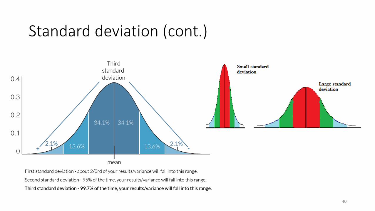
Standard deviation (cont.)

40

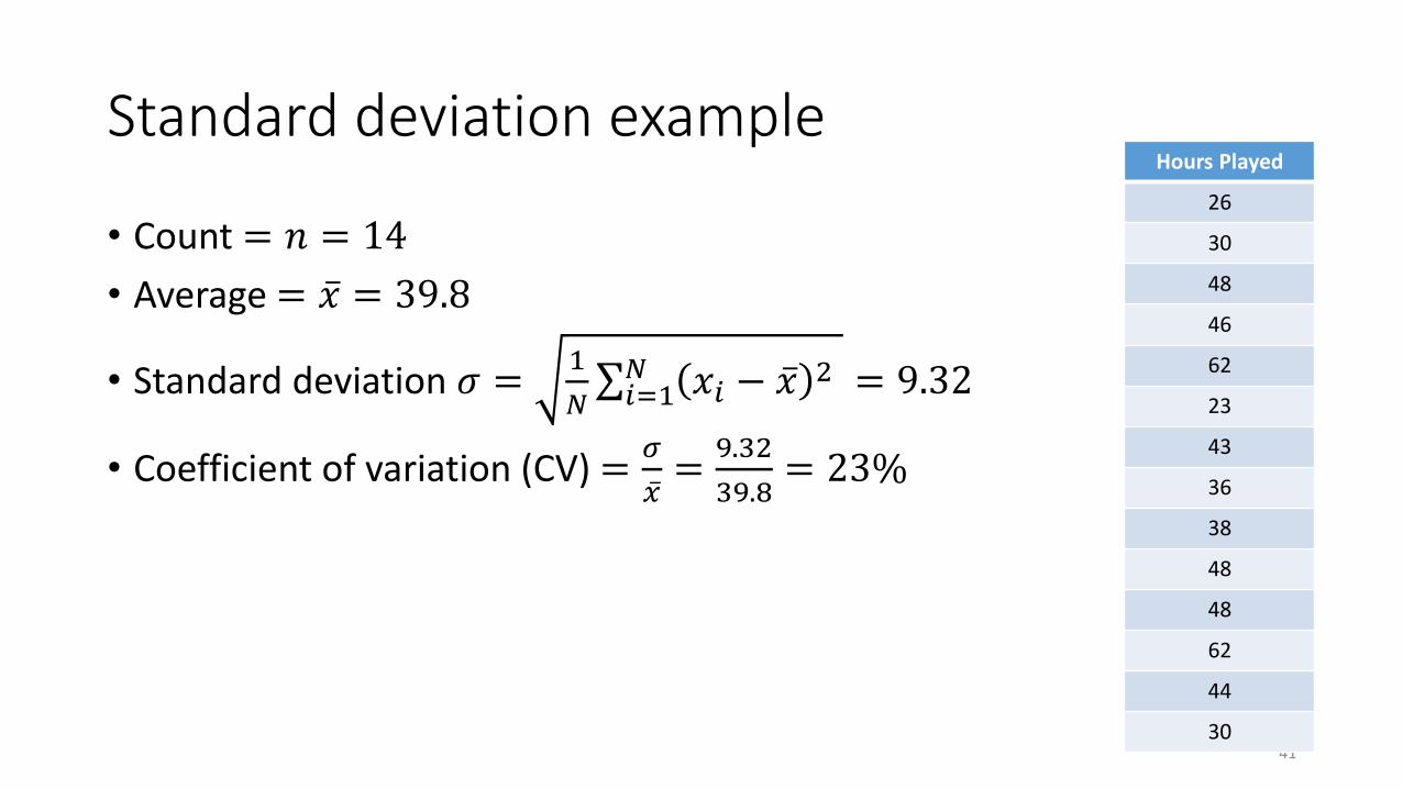
Standard deviation example

• Count = 𝑛 = 14

• Average = ҧ𝑥 = 39.8

• Standard deviation 𝜎 =1

𝑁σ𝑖=1𝑁 𝑥𝑖 − ҧ𝑥 2 = 9.32

• Coefficient of variation (CV) =𝜎

ҧ𝑥=

9.32

39.8= 23%

41

Hours Played

26

30

48

46

62

23

43

36

38

48

48

62

44

30

Standard deviation example (cont.)

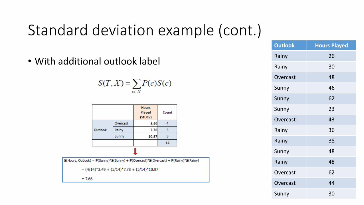
• With additional outlook label

42

Outlook Hours Played

Rainy 26

Rainy 30

Overcast 48

Sunny 46

Sunny 62

Sunny 23

Overcast 43

Rainy 36

Rainy 38

Sunny 48

Rainy 48

Overcast 62

Overcast 44

Sunny 30

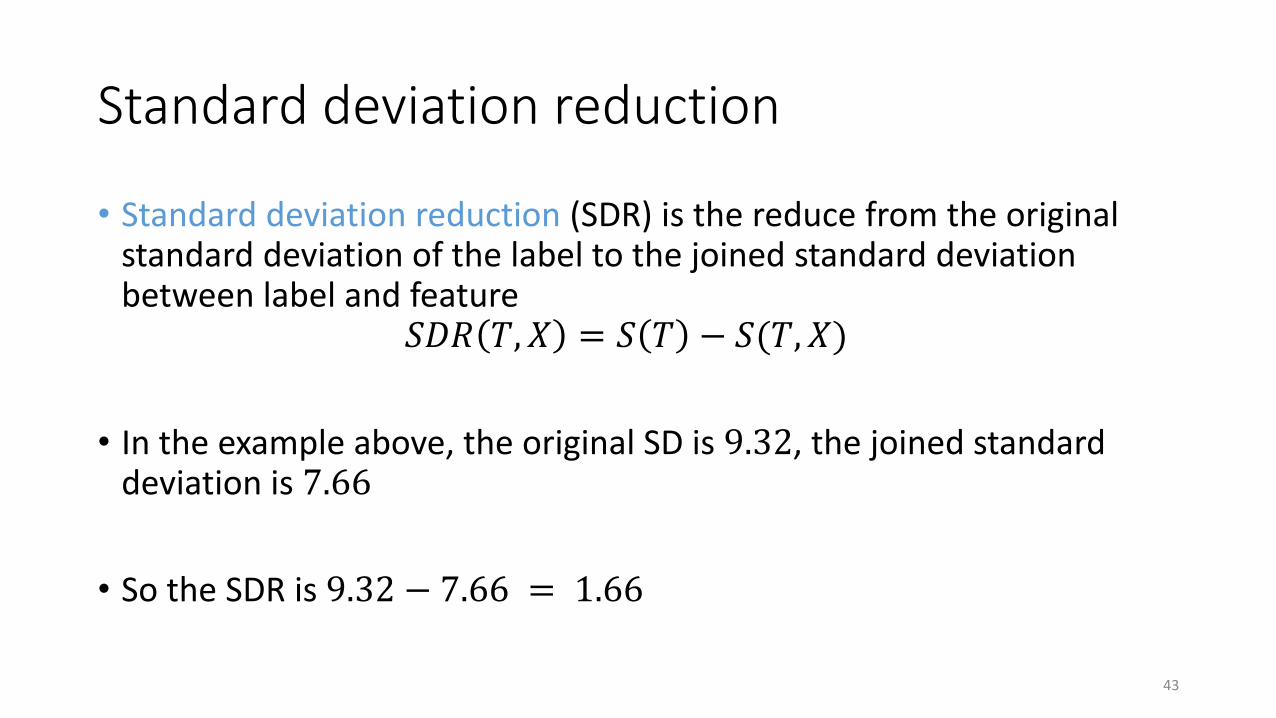
Standard deviation reduction

• Standard deviation reduction (SDR) is the reduce from the original standard deviation of the label to the joined standard deviation between label and feature

𝑆𝐷𝑅 𝑇, 𝑋 = 𝑆 𝑇 − 𝑆(𝑇, 𝑋)

• In the example above, the original SD is 9.32, the joined standard deviation is 7.66

• So the SDR is 9.32 − 7.66 = 1.66

43

Complete example dataset

44

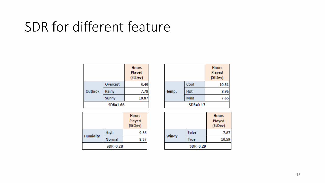
SDR for different feature

45

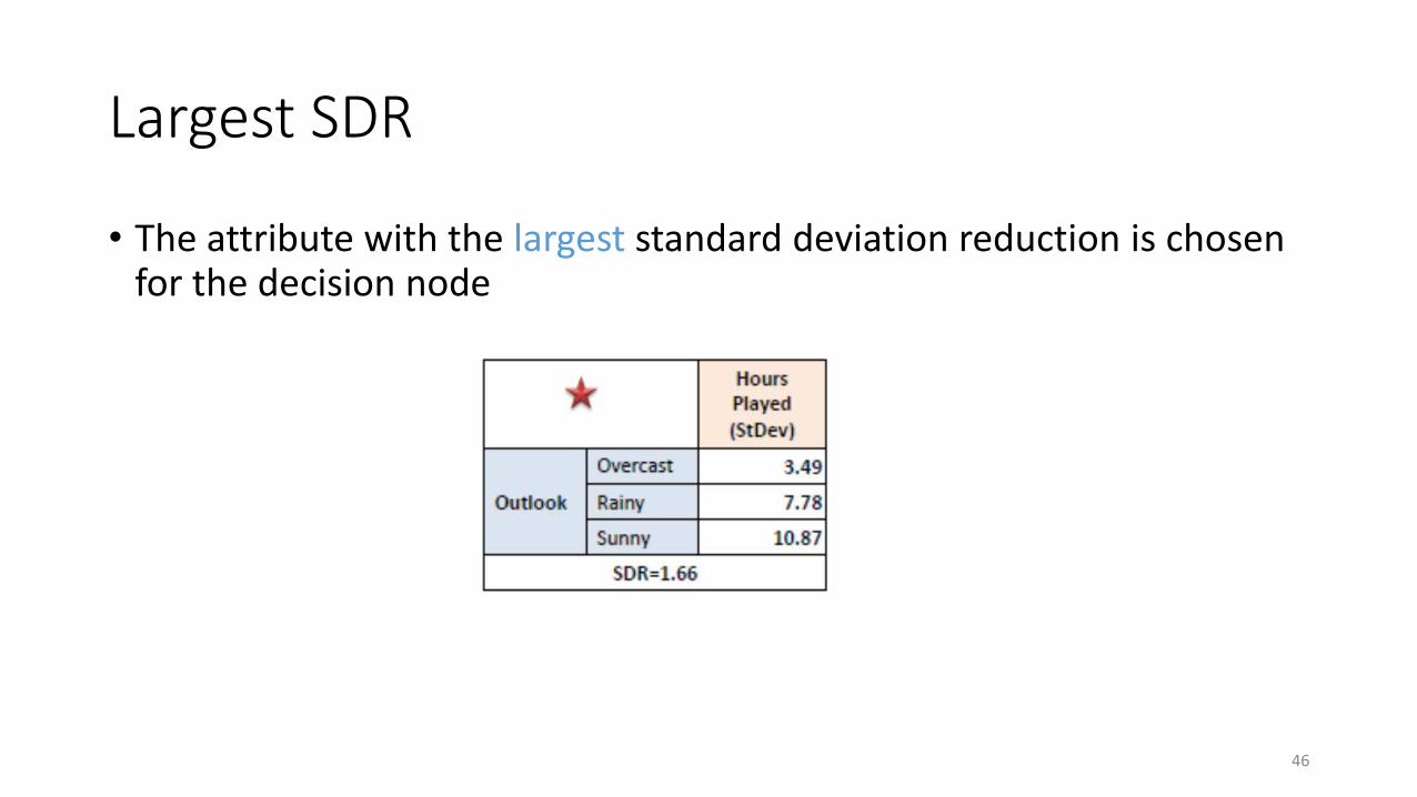
Largest SDR

• The attribute with the largest standard deviation reduction is chosen for the decision node

46

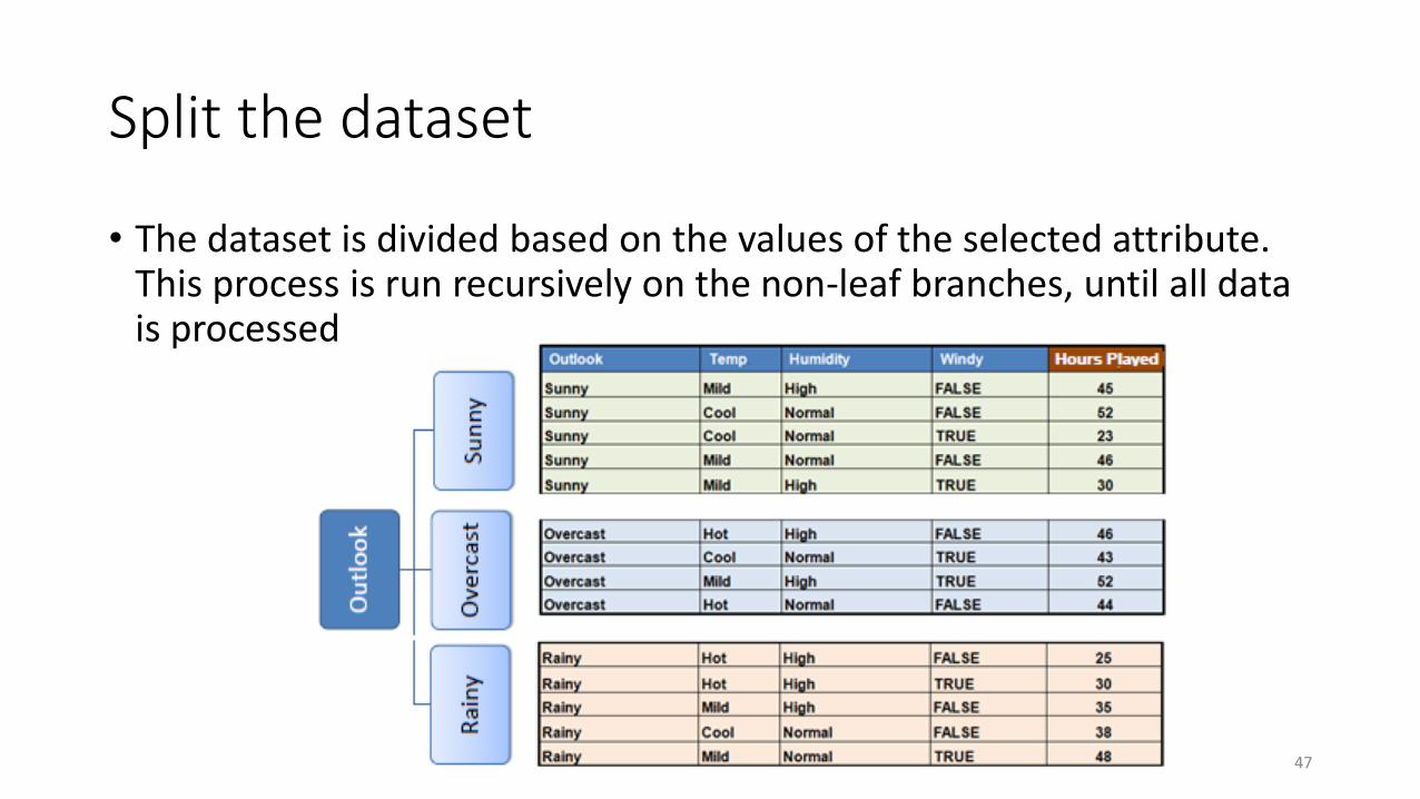
Split the dataset

• The dataset is divided based on the values of the selected attribute. This process is run recursively on the non-leaf branches, until all data is processed

47

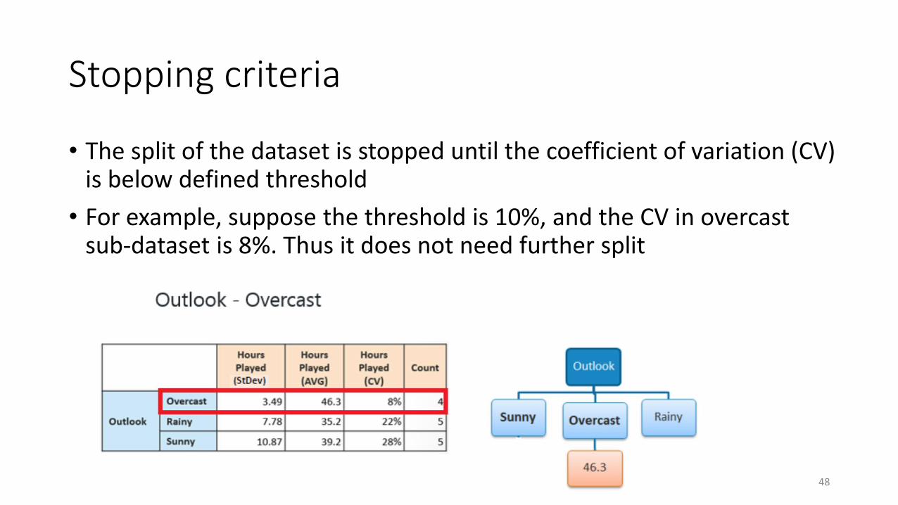
Stopping criteria

• The split of the dataset is stopped until the coefficient of variation (CV) is below defined threshold

• For example, suppose the threshold is 10%, and the CV in overcast sub-dataset is 8%. Thus it does not need further split

48

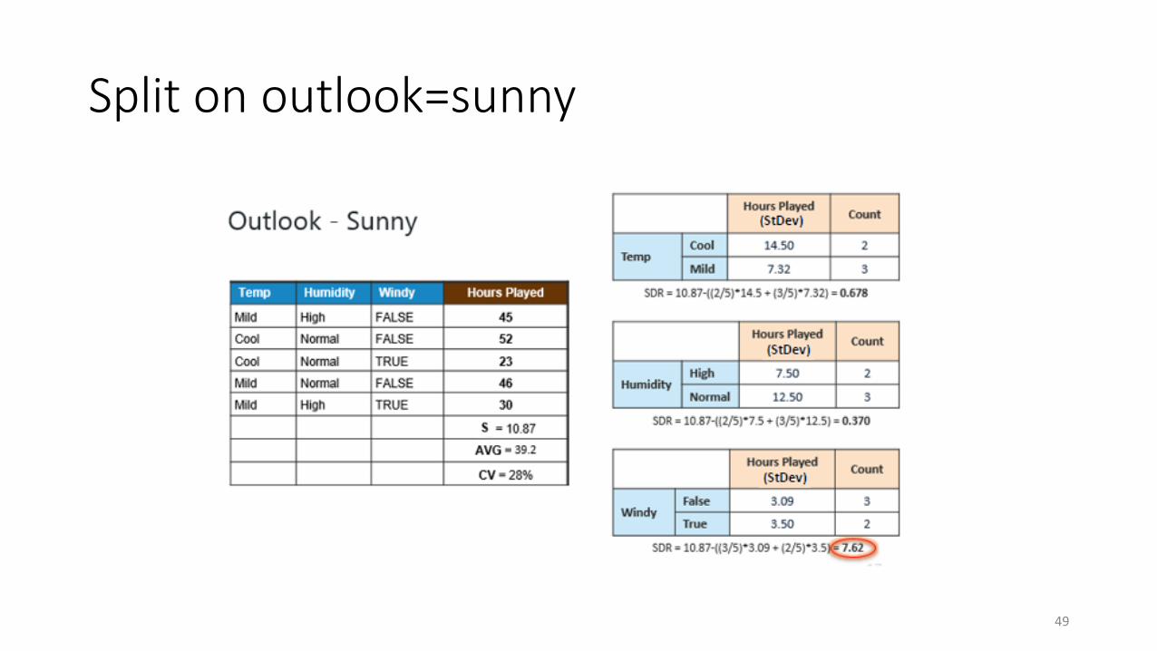
Split on outlook=sunny

49

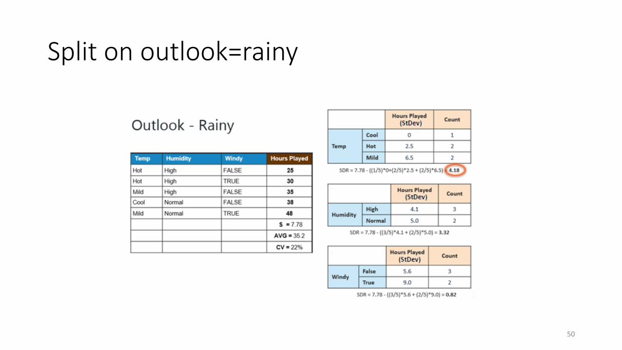
Split on outlook=rainy

50

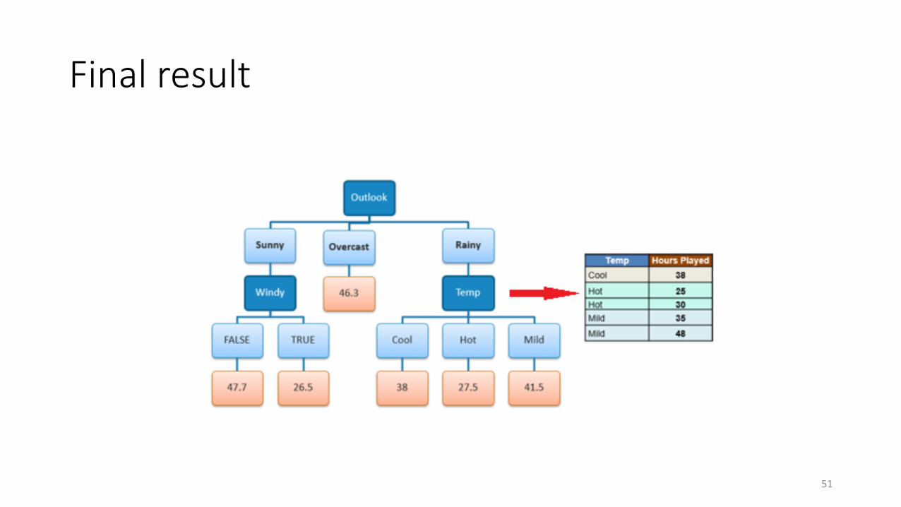
Final result

51

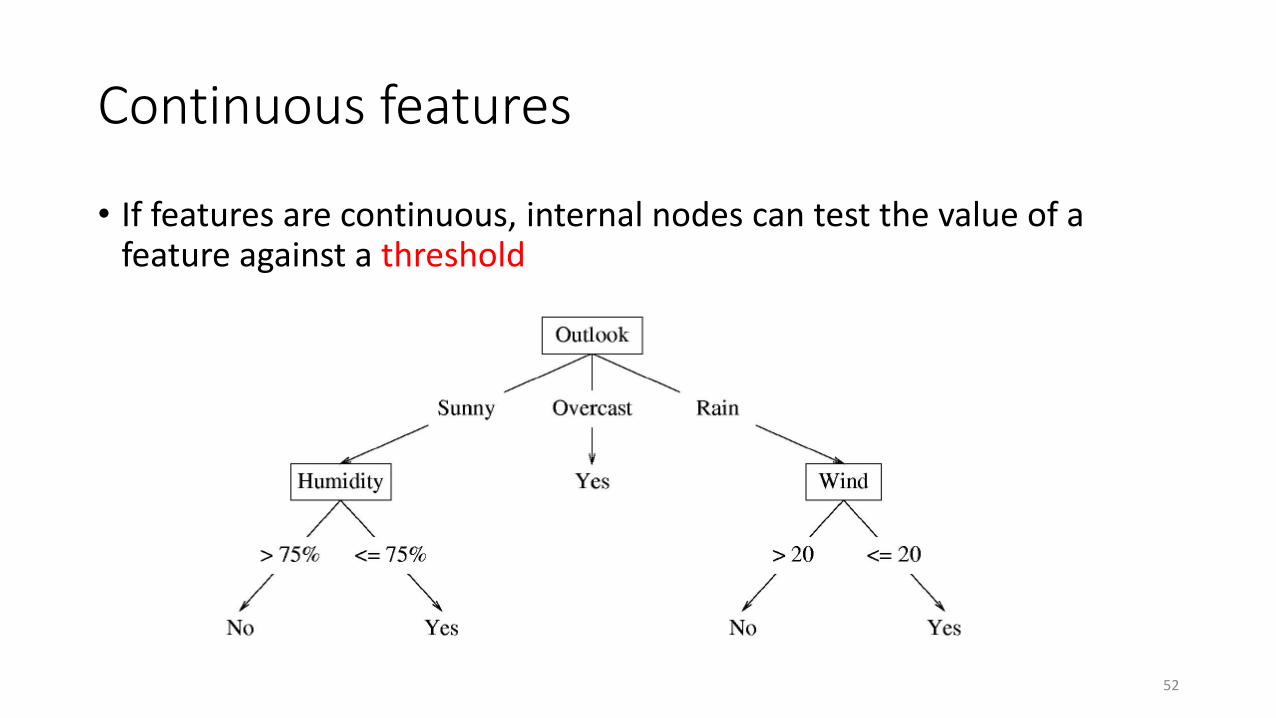
Continuous features

• If features are continuous, internal nodes can test the value of a feature against a threshold

52

Summary

Decision Tree Features

Discrete Continuous

Labels Discrete Information Gain (IG)

Continuous Standard Deviation Reduction (SDR)

53