LECTURE NOTES 16 - University of Illinois at Urbana ...web.hep.uiuc.edu/home/serrede/P436/Lecture_Notes/P436_Lect_16.pdf · UIUC Physics 436 EM Fields & Sources II Fall Semester,

UIUC Physics 436 EM Fields & Sources II Fall Semester, 2015 Lect. Notes 16 Prof. Steven Errede

© Professor Steven Errede, Department of Physics, University of Illinois at Urbana-Champaign, Illinois 2005-2015. All Rights Reserved.

1

LECTURE NOTES 16

THE STRUCTURE OF SPACE-TIME

Lorentz Transformations Using Four-Vectors:

Space-time {as we all know…} has four dimensions: 1 time dimension & 3 {orthogonal} spatial dimensions: ˆ ˆ ˆ, t r xx yy zz

.

Einstein’s Theory of (Special) Relativity:

1-D time and 3-D space are placed on an equal/symmetrical footing with each other.

We use 4-vector/tensor notation for relativistic kinematics and relativistic electrodynamics because the mathematical description of the physics takes on a simpler, and more elegant appearance; the principles and physical consequences of the physics are also made clearer/more profound!

Lorentz Transformations Expressed in 4-Vector Notation:

Note the contravariant superscripts, here!

We define any 4-vector: 0 1 2 3, , ,x x x x x

Where, by convention: the 0th component of the 4-vector, x0 = is the temporal (time-like), {i.e. scalar} component of the 4-vector x , and (x1, x2, x3) are the (x, y, z) spatial (space-like) {i.e. 3-vector} components of the 4-vector x , respectively.

n.b. Obviously, the physical SI units of a 4-vector components must all be the same!!!

For space-time 4-vectors, we define contravariant/superscript x as:

0

1

2

3

x ct

x x

x y

x z

0 1 2 3, , , , , ,x x x x x ct x y z

Then the Lorentz transformation of space-time quantities in IRF(S) to IRF(S´), the latter of which is moving e.g. with velocity ˆv vx

relative to IRF(S) is given by:

ct ct x

x x ct

y y

z z

0 0 1

1 1 0

2 2

3 3

x x x

x x x

x x

x x

Where: vc and:

2

1

1

Original 4-vector Notation:

New/Tensor 4-vector Notation



2

We can also write these four equations (either version) in matrix form as:

0 0

0 0

0 0 1 0

0 0 0 1

ct ct

x x

y y

z z

or:

0 0

1 1

2 2

3 3

0 0

0 0

0 0 1 0

0 0 0 1

x x

x x

x x

x x

Each of the four above equations of the RHS representation can also be written compactly and elegantly in tensor notation as:

3

0

x x

where: μ = 0, 1, 2, 3 and: Λ Lorentz Transformation Matrix

0 0 0 00 1 2 31 1 1 10 1 2 32 2 2 20 1 2 33 3 3 30 1 2 3

0 0

0 0

0 0 1 0

0 0 0 1

superscript, μ = 0, 1, 2, 3 = row index

where: throwcolumn v

element of Λ

subscript, v = 0, 1, 2, 3 = column index

We explicitly write out each of the four equations associated with3

0

v

v

x x

for μ = 0, 1, 2, 3:

3

0 0 0 0 0 1 0 2 0 3 0 10 1 2 3

0

x x x x x x x x

3

1 1 1 0 1 1 1 2 1 3 1 00 1 2 3

0

x x x x x x x x

32 2 2 0 2 1 2 2 2 3 2

0 1 2 30

x x x x x x x

33 3 3 0 3 1 3 2 3 3 3

0 1 2 30

x x x x x x x

We can write this relation even more compactly using the Einstein summation convention: Repeated indices are always summed over:

3

0

v v

v

x x x

The RHS of this equation has repeated index v, which implicitly means we are to sum over it, i.e.

Thus: vx x is simply shorthand notation for:

3

0

v

v

x x

row index

column index

People (including Einstein) got / get tired of explicitly writing all of the

summation symbols 3

0v all the time /

everywhere….



3

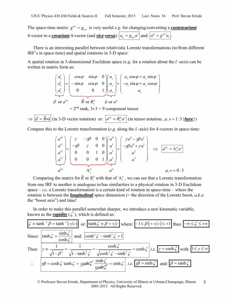
The nature/composition of the Lorentz transformation matrix Λ (a rank-two, 4 x 4 = 16 component tensor) defines the space-time structure of our universe, i.e. specifies the rules for transforming from one IRF to another IRF.

Generally speaking mathematically, one can define a 4-vector a to be anything one wants, however for special relativity and Lorentz transformations between one IRF and another, our 4-vectors are only those which transform from one IRF to another IRF as:

3

0

vv

v

a a

vva a

This compact relation mathematically defines the space-time nature/structure of our universe!

For a Lorentz transformation along the ˆ ˆ1 x axis, with: ˆv vx

and thus: x

, v c

for a 4-vector 0 1 2 3, , ,a a a a a , where 0a is the temporal/scalar component and

1 2 3, , , ,x y za a a a a a a

are the ˆ ˆ ˆ, ,x y z spatial/3-vector components of the 4-vector a ,

then vva a written out in matrix form is:

0 10 0

1 1 1 0

2 22

3 33

0 0

0 0

0 0 1 0

0 0 0 1

a aa a

a a a aa a aa a a

Dot Products with 4-Vectors:

In “standard” 3-D space-type vector algebra, we have the familiar scalar product / dot product:

ˆ ˆ ˆ ˆˆ ˆx y z x y z x x y y z za b a x a y a z b x b y b z a b a b a b = scalar quantity (i.e. = pure #)

A relativistic 4-vector analog of this, but it is NOT simply the sum of like components.

Instead, the zeroth component product of a relativistic 4-vector dot product has a minus sign:

0 0 1 1 2 2 3 3a b a b a b a b four-dimensional scalar product / dot product ( = pure #)

Just as an ordinary / “normal” 3-D vector product a b is invariant (i.e. unchanged) under

3-D space rotations ( a b is the length of vector b

projected onto a

{and/or vice versa} – a

length does not change under a 3-D space rotation), the four-dimensional scalar product between two relativistic 4-vectors is invariant (i.e. unchanged) under any/all Lorentz transformations, from one IRF(S) to another IRF(S′).

i.e. The scalar product/dot product of any two relativistic 4-vectors is a Lorentz invariant quantity. The scalar product/dot product of any two relativistic 4-vectors has the same numerical value in any/all IRFs !!!



4

Thus: 0 0 1 1 2 2 3 3a b a b a b a b = 0 0 1 1 2 2 3 3a b a b a b a b = pure #

In IRF(S′) In IRF(S)

In order to keep track of the minus sign associated with the temporal component of a 4-vector, especially when computing a scalar/dot product, we introduce the notion of contravariant and covariant 4-vectors.

What we have been using thus far in these lecture notes are contravariant 4-vectors a , denoted by the superscript μ:

0 1 2 3, , ,a a a a a = contravariant 4-vector:

A covariant 4-vector a is denoted by its subscript μ:

0 1 2 3, , ,a a a a a = covariant 4-vector: 0 1 2 3columna a a a a a

The temporal/zeroth component {only} of covariant a differs from that of contravariant a

by a minus sign: 0

01

12

23

3

a a

a a

a a

a a

Thus, raising {or lowering} the index μ of a 4-vector, e.g. a a or a a

changes the

sign of the zeroth (i.e. temporal/scalar) component of the 4-vector {only}.

That’s why we have to pay very close attention to subscripts vs. superscripts here !!!

Thus, a 4-vector scalar/dot product ( = a Lorentz invariant quantity) may be written using contravariant and covariant 4-vectors as:

3 3

0 0

a b a b

= 0 1 2 3

0 1 2 3a b a b a b a b = 0 1 2 3

0 1 2 3a b a b a b a b = pure #

This {again} can be written more compactly / elegantly / succinctly using the Einstein summation convention (i.e. summing over repeated indices) as:

a b a b =

0 1 2 30 1 2 3a b a b a b a b =

0 1 2 30 1 2 3a b a b a b a b = pure #

We define the 4-D “flat” space-time metric vvg g

:

1 0 0 0

0 1 0 0

0 0 1 0

0 0 0 1

vvg g

with: g g

Note: the above definition of the metric vvg g

is not universal in the literature/textbooks…

Same sign for both contravariant and covariant 4-vectors

0

1

2

3

row

a

aa a

a

a

Note the – sign difference !!!

is the 4-D space-time version of

the 3-D Kroenecker -function ij ,

i.e. 0 if and

1 for 0,1,2,3 .



5

The space-time metric vvg g

is very useful e.g. for changing/converting a contravariant

4-vector to a covariant 4-vector (and vice-versa): vva g a and: v

va g a .

There is an interesting parallel between relativistic Lorentz transformations (to/from different IRF’s in space-time) and spatial rotations in 3-D space:

A spatial rotation in 3-dimensional Euclidean space (e.g. for a rotation about the z -axis) can be written in matrix form as:

cos sin 0 cos sin

sin cos 0 sin cos

0 0 1

x x x y

y y x y

z z z

a a a a

a a a a

a a a

or a a or vR R

or a a

= 2nd rank, 33 = 9 component tensor

a R a (in 3-D vector notation) or: v

va R a (in tensor notation, , 1: 3v {here})

Compare this to the Lorentz transformation (e.g. along the x -axis) for 4-vectors in space-time:

0 0 0 1

1 1 0 1

2 2 2

3 3 3

0 0

0 0

0 0 1 0

0 0 0 1

a a a a

a a a a

a a a

a a a

vva a

a v a , 0 : 3v

Comparing the matrix for or vR R

with that of v , we can see that a Lorentz transformation

from one IRF to another is analogous to/has similarities to a physical rotation in 3-D Euclidean space – i.e. a Lorentz transformation is a certain kind of rotation in space-time – where the rotation is between the longitudinal space dimension (= the direction of the Lorentz boost, a.k.a. the “boost axis”) and time!

In order to make this parallel somewhat sharper, we introduce a new kinematic variable, known as the rapidity ( ), which is defined as:

1 1tanh tanh v c or: tanh v c where: 1 1v c thus:

Since: sinh

tanhcosh

and: 2 2cosh sinh 1

Then: 2 2 2 2

1 1 coshcosh

1 1 tanh cosh sinh

i.e. cosh with: 1

cosh tanh cosh sinh

cosh

sinh i.e. sinh and: tanh



6

Since: 2 2cosh sinh 1 we also see that: 2 2 2 1 . {Obvious, since:

22

1

1

}

Thus, the Lorentz transformation (along the x -axis) vva a of a 4-vector a can be written

{using tanh , cosh and sinh } as:

0 0 0 0 1

1 1 1 0 1

2 2 2 2

3 3 3 3

0 0 cosh sinh 0 0 cosh sinh

0 0 sinh cosh 0 0 sinh cosh

0 0 1 0 0 0 1 0

0 0 0 1 0 0 0 1

a a a a a

a a a a a

a a a a

a a a a

Again, compare this with the 3-D space rotation of a 3-D space-vector a

about the z -axis:

cos sin 0 cos sin

sin cos 0 sin cos

0 0 1

x x x y

y y x y

z z z

a a a a

a a a a

a a a

We see that the above Lorentz transformation is similar (but not identical) to the expression for the 3-D Euclidean geometry spatial rotation!

However, because of the sinh and cosh nature associated with the Lorentz transformation we see that the Lorentz transformation is in fact a hyperbolic rotation in space-time – i.e. the transformation of the longitudinal space dimension associated with the axis parallel to the Lorentz boost direction and time is that of a hyperbolic-type rotation!!!

The use of the rapidity variable, has benefits e.g. for the Einstein Velocity Addition Rule:

If u dx dt

= the velocity of a particle as seen by an observer in IRF(S) and u dx dt

= the velocity of the particle as seen by an observer in IRF(S') and ˆv vx

= the relative velocity

between IRF(S) and IRF(S'), then u is related to u by:

21

u vu

uv c

Einstein Velocity Addition Rule (1-D Case)

We can re-write this as: 21

u c v cu c

uv c

1

uu

u

Then since: tanh we can similarly define: tanhu u and tanhu u .

Then: 1

uu

u

tanh tanh

tanh tanh1 tanh tanh

uu u

u

Thus: tanh tanhu u

Or: u u Rapidity form of the Einstein Velocity Addition Rule (1-D Case)

Rapidities 1tanh are additive quantities in going from one IRF to another IRF !!!

See e.g. CRC Handbook r.e. trigonometric identities for hyperbolic functions!



7

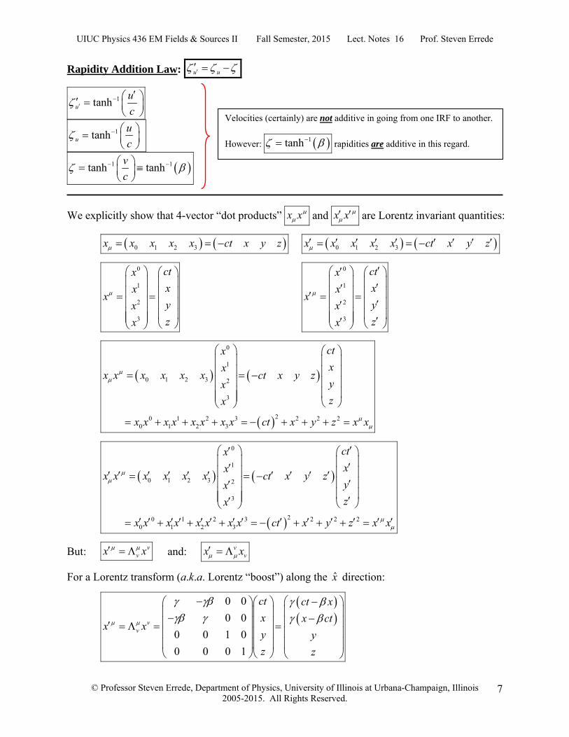
Rapidity Addition Law: u u

1tanhu

u

c

1tanh u

u

c

1 1tanh tanhv

c

We explicitly show that 4-vector “dot products” x x and x x

are Lorentz invariant quantities:

0 1 2 3x x x x x ct x y z 0 1 2 3x x x x x ct x y z

0

1

2

3

ctx

xxx

yx

zx

0

1

2

3

ctx

xxx

yx

zx

0

1

0 1 2 3 2

3

20 1 2 3 2 2 20 1 2 3

ctx

xxx x x x x x ct x y z

yx

zx

x x x x x x x x ct x y z x x

0

1

0 1 2 3 2

3

20 1 2 3 2 2 20 1 2 3

ctx

xxx x x x x x ct x y z

yx

zx

x x x x x x x x ct x y z x x

But: vvx x and: v

vx x

For a Lorentz transform (a.k.a. Lorentz “boost”) along the x direction:

0 0

0 0

0 0 1 0

0 0 0 1

vv

ct ct x

x x ctx x

y y

z z

Velocities (certainly) are not additive in going from one IRF to another.

However: 1tanh rapidities are additive in this regard.



8

And:

0 0

0 0

0 0 1 0

0 0 0 1

vvx x ct x y z ct x x ct y z

Thus:

2 22 2 2 2

2 22 2 2 2 2 2 2 2

22 2

2 2

2

ct x

x ctx x ct x x ct y z

y

z

ct x x ct y z

ct xct x x xct ct y z

ct xct

2 2 2 2 2 22x x xct

22 2 2 2

2 22 2 2 2 2 2 2 2 2 2

22 2 2 2 2 2 2

1 1

ct y z

ct ct x x y z

ct x y z

But: 2 21 1

2

2

1

1x x

2

2

2

1

1ct

22 2 2 2 2 2x y z ct x y z

i.e. 2 22 2 2 2 2 2x x x x ct x y z ct x y z x x x x

x x x x = x x x x

are indeed Lorentz invariant quantities!

Lorentz Transformations from the Lab Frame IRF(S) to a Moving Frame IRF(S'):

1.) 1-D Lorentz Transform / “Boost” along the x direction: xx

v

c

2

1

1 x

0

1

2

3

0 0

0 0

0 0 1 0

0 0 0 1

x x

xv xv

ct ct ct xx

x x x ctxx x

y y yx

z z zx



9

2.) 1-D Lorentz Transform / “Boost” along the y direction: yy

v

c

2

1

1 y

0

1

2

3

0 0

0 1 0 0

0 0

0 0 0 1

yy

vv

y y

ct yct ctx

x x xxx x

y yx y ctz zx z

3.) 1-D Lorentz Transform / “Boost” along the z direction: zz

v

c

2

1

1 z

0

1

2

3

0 0

0 1 0 0

0 0 1 0

0 0

zz

vv

zz

ct zct ctx

xx xxx x

yy yx

z ctz zx

4.) 3-D Lorentz Transform / “Boost” along arbitrary r direction: v

c

2

1

1

First, we define: ˆ ˆ ˆr xx yy zz

2 2 2 r r x y z

ˆ ˆ ˆx y zv v x v y v z

In IRF(S) 2 2 2 x y zv v v v v

v

c

ˆ ˆ ˆx y zx y z

2 2 2

x y z

Then:

2

02 2 2

12

22 2 2

3

2

2 2 2

11 11

1 1 11

11 11

x y z

x yx x zx

vv x y y y z

y

y zx z zz

ct ctx

x xxx x

y yx

z zx

{n.b. By inspection of this 3-D -matrix for 1-D motion (i.e. only along ˆ ˆ, ,x y or z ) it is easy to show that this expression reduces to the appropriate 1-D Lorentz transformation 1.) – 3.) above.}



10

Or:

0

21

2

23

2

1

1

1

x x

vv

y y

z z

ct r

ctx x r ctxx

x xyx y r ctzx

z r ct

with: 2 2 2

2

ˆ ˆ ˆ

1

1

x y z

x y z

x y z

n.b. The 0x ct equation follows trivially from 0x ct in 1.) through 3.) above.

The 3-D spatial part can be written vectorially as: 2

1r r r ct

which may appear to be a more complicated expression, but it’s really only sorting out components of and r r

that are and to v

for separate treatment.

Thus, we can write the 3-D Lorentz transformation from the lab frame IRF(S) to the moving frame IRF(S) along an arbitrary direction r with relative velocity ˆv vr

elegantly and compactly as:

2

1

ct rct

r r r ct

See J.D. Jackson’s “Electrodynamics”, 3rd Edition, p. 525 & p. 547 for more information. Inverse Lorentz Transformations from a Moving Frame IRF(S') to the Lab Frame IRF(S):

1'.) 1-D Lorentz Transform / “Boost” along the x direction: x xx x

v v

c c

2

1

1 x

0

1

2

3

0 0

0 0

0 0 1 0

0 0 0 1

x x

xv xv

ct ct ct xx

x x x ctxx x

y y yx

z z zx

2'.) 1-D Lorentz Transform / “Boost” along the ydirection: y yy y

v v

c c

2

1

1 y

0

1

2

3

0 0

0 1 0 0

0 0

0 0 0 1

yy

vv

y y

ct yct ctx

x x xxx x

y yx y ctz zx z



11

3'.) 1-D Lorentz Transform / “Boost” along the zdirection: z zz z

v v

c c

2

1

1 z

0

1

2

3

0 0

0 1 0 0

0 0 1 0

0 0

zz

vv

zz

ct zct ctx

xx xxx x

yy yx

z ctz zx

4'.) 3-D Lorentz Transform / “Boost” along arbitrary r direction:v v

c c

2

1

1

First, we define: ˆ ˆ ˆr x x y y z z

2 2 2 r r x y z

ˆ ˆ ˆx y zv v x v y v z v

In IRF(S') 2 2 2 x y zv v v v v v

v v

c c

ˆ ˆ ˆ

ˆ ˆ ˆ

x y z

x y z

x y z

x y z

2 2 2

2 2 2

x y z

x y z

Then:

2

02 2 2

12

22 2 2

3

2

2 2 2

11 11

1 1 11

11 11

x y z

x yx x zx

vv x y y y z

y

y zx z zz

ct ctx

x xxx x

y yx

z zx

{n.b. By inspection of this 3-D -matrix for 1-D motion (i.e. only along ˆ ˆ, ,x y or z ) it is easy to show that this expression reduces to the appropriate 1-D Lorentz transformation 1'.) – 3'.) above.}

Or:

0

21

2

23

2

1

1

1

x x

vv

y y

z z

ct r

ctx x r ctxx

x xyx y r ctzx

z r ct

with: 2 2 2

2

ˆ ˆ ˆ

1

1

x y z

x y z

x y z



12

n.b. The 0x ct equation follows trivially from 0x ct in 1'.) through 3'.) above.

The 3-D spatial part can be written vectorially as: 2

1r r r ct

which may appear to be a more complicated expression, but it’s really only sorting out components of and r r

that are and to v for separate treatment.

Thus, we can write the 3-D Lorentz transformation from the moving frame IRF(S) to the lab frame IRF(S) along an arbitrary direction r with relative velocity ˆv vr

elegantly and compactly as:

2

1

ct rct

r r r ct

Note also that: vvx x but: v vx x . v v

v vx x x

The quantity: 1vv

= identity (i.e. unit) 44 matrix =

1 0 0 0

0 1 0 0

0 0 1 0

0 0 0 1

Thus: 1v vv vx x x x x

i.e. 1v vv v

We define the relativistic space-time interval between two “events” as the

Space-time difference: A Bx x x ← known as the space-time displacement 4-vector

Event A occurs at space-time coordinates:

0

1

2

3

AA

AAA

AA

AA

ctx

xxx

yx

zx

Event B occurs at space-time coordinates:

0

1

2

3

BB

BBB

BB

BB

ctx

xxx

yx

zx

The scalar 4-vector product of x x x x is a Lorentz-invariant quantity,

= same numerical value in any IRF, also known as the interval I between two events:

n.b. Lorentz-invariant

quantity!!!



13

Lorentz-Invariant Interval: I x x x x = same numerical value in all IRF’s.

2 2 2 2 2 2 2 20 1 2 3 2

2 2 2 2 2

AB AB AB AB

A B A B A B A B

t x y z

AB AB AB AB

I x x x x c t t x x y y z z

c t x y z

Define the usual 3-D spatial distance: 2 2 2AB AB AB ABd x y z

2 2 2 2 2 2 2 2AB AB AB AB AB ABI x x x x c t x y z c t d

←

Thus, when Lorentz transform from one IRF(S) to another IRF(S′):

In IRF(S): 2 2 2AB ABI x x x x c t d

In IRF(S′): 2 2 2AB ABI x x x x c t d

Because the interval I is a Lorentz-invariant quantity, then:

I x x x x = I x x x x

Or: 2 2 2AB ABc t d = 2 2 2

AB ABc t d

Work this out / prove to yourselves that it is true → follow procedure / same as on pages 7-8 of these lecture notes.

Note that: ( ) ( )

AB ABIRF S IRF S

t t

and ( ) ( )

AB ABIRF S IRF S

d d

Time dilation in IRF(S′) relative to IRF(S) is exactly compensated by spatial Lorentz contraction in IRF(S′) relative to IRF(S), keeping the interval I the same (i.e. Lorentz invariant) in all IRF’s !

Profound aspect / nature of space-time!

Depending on the details of the two events (A & B), the interval 2 2 2

AB ABI x x x x c t d can be positive, negative, or zero:

I < 0: Interval I is time-like: 2 2 2AB ABc t d

e.g. If two events A & B occur at same spatial location, then: A Br r

→ 0ABd ,

The two events A & B must have occurred at different times, thus: 0ABt .

I > 0: Interval I is space-like: 2 2 2AB ABc t d

e.g. If two events A & B occur simultaneously, then: A Bt t → 0ABt ,

The two events A & B must have occurred at different spatial locations, thus: 0ABd .

I = 0: Interval I is light-like: 2 2 2AB ABc t d

e.g. The two events A & B are connected by a signal traveling at the speed of light (in vacuum).

Lorentz-invariant quantity, same numerical

value in all IRF’s



14

Space-time Diagrams Minkowski Diagrams:

On a “normal”/Galilean space-time diagram, we plot x(t) vs. t:

speed, v(t) = local slope

t

dx t

dt

of x(t) vs. t graph at time t.

In relativity, we {instead} plot ct vs. x (danged theorists!!!) for the space-time diagram: (a.k.a. Minkowski diagram)

Dimensionless speed :

1 1

slope

x

v

c d ct

dx

of ct vs. x graph at point x.

A particle at rest in an IRF is represented by a vertical line on the relativistic space-time diagram:

slope

Ax x

d ct

dx

1 10

slope

The “trajectory” of a particle in the space-time diagram makes an angle θ = 0o with respect to vertical (ct) axis.

A photon traveling at v = c is represented by a straight line at 45o with respect to the vertical (ct) axis:

slope

1Ax x

d ct

dx

1 11

1photon slope

(i.e. photonv c )



15

A particle traveling at constant speed v < c (β < 1) is represented by a straight line making an angle θ < 45o with respect to the vertical (ct) axis:

slope

1Ax x

d ct

dx

1 11

1particle slope

i.e. vparticle < c

particleparticle

vc

c

The trajectory {i.e. locus of space-time points} of a particle on a relativistic space-time / Minkowski diagram is known as the world line of the particle.

All three of the above situations superimposed together on the Minkowski/space-time diagram: Suppose you set out from t = 0 at the origin of your own Minkowski diagram. Because your speed can never exceed c ( v c , i.e. 1 ), your trajectory (your world line) in the ct vs. x space-time diagram can never have |slope| = |d(ct)/dx| < 1, anywhere along it.

Your “motion” in the Minkowski diagram is restricted to the wedge-shaped region bounded by the two 45o lines (with respect to vertical (ct) axis) as shown in the figure below:



16

The ±45o wedge-shaped region above the horizontal x-axis (ct > 0) is your future at t = 0 = locus of all space-time points potentially accessible to you.

Of course, as time goes on, as you do progress along your world line, your “options” progressively narrow – your future at any moment t > 0 is the ±45o wedge constructed from / at whatever space-time point (ctA, xA) you are at, at that point in space (xA) at the time tA.

The backward ±45o wedge below the horizontal x-axis (ct < 0) is your past at t = 0 = locus of all points potentially accessed by you in the past.

The space-time regions outside the present and past ±45o wedges in the Minkowski diagram are inaccessible to you, because you would have to travel faster than speed of light c to be in such regions!

A space-time diagram with one time dimension (vertical axis) and 3 space dimensions (3 horizontal axes: x, y and z) is a 4-dimensional diagram – can’t draw it on 2-D paper!

In a 4-D Minkowski Diagram, ±45o wedges become 4-D “hypercones” (aka light cones). “future” = contained within the forward light cone. “past” = contained within the backward light cone.

The slope of the world line/the trajectory connecting two events on a space-time diagram tells

you at a glance whether the invariant interval I x x x x is:

a) Time-like (slope

1d ct

dx ) (all points in your future and your past are time-like)

b) Space-like (slope

1d ct

dx ) (all points in your present are space-like)

c) Light-like (slope

1d ct

dx ) (all points on your light cone(s) are light-like)



17

Changing Views of Relativistic Space-time Along the World line of a Rapidly Accelerating Observer

For relativistic space-time, the vertical axis is ctime, the horizontal axis is distance; the dashed line is the space-time trajectory ("world line") of the observer. The small dots are arbitrary events in space-time. The lower quarter of the diagram (within the light cone) shows events (dots) in the past that were visible to the user, the upper quarter (within the light cone) shows events (dots) in the future that the observer will be able to see. The slope of the world line (deviation from vertical) gives the relative speed to the observer. Note how the view of relativistic space-time changes when the observer accelerates {see relativistic animation}.

Changing Views of Galilean Space-time Along the World Line of a Slowly Accelerating Observer

In non-relativistic Galilean/ Euclidean space, the vertical axis is ctime, the horizontal axis is distance; the dashed line is the space-time trajectory ("world line") of the observer. The small dots are arbitrary events in space-time. The lower half of the diagram shows (past) events that are "earlier" than the observer, the upper half shows (future) events that are "later" than the observer. The slope of the world line (deviation from vertical) gives the relative speed to the observer. Note how the view of Galilean / Euclidean space-time changes when the observer accelerates {see Galilean animation}.



18

Note that time in space-time is not “just another coordinate” (like x, y, z) – its “mark of distinction” is the minus sign in the invariant interval:

2 2 2 2I x x x x c t x y z

The minus sign in the invariant interval (arising from / associated with time dimension) imparts a rich structure to sinh, cosh, tanh . . . the hyperbolic geometry of relativistic space-time versus the circular geometry of Euclidean 3-dimensional space.

In Euclidean 3-D space, a rotation {e.g. about the z -axis} of a point P in the x-y plane

describes a circle – the locus of all points at a fixed distance 2 2r x y from the origin:

r = constant (i.e. is invariant) under a rotation in Euclidean / 3-D space. For a Lorentz transformation in relativistic space-time, the interval

2 2 2 2I x x x x c t x y z is a Lorentz-invariant quantity

(i.e. is preserved under any/all Lorentz transformations from one IRF to another).

The locus of all points in space-time with a given / specific value of I is a hyperbola

(for ct and x (i.e. 1 space dimension) only): 2 2I c t x

If we include e.g. the y -axis, the locus of all points in space-time with a given / specific

value of 2 2 2I c t x y is a hyperboloid of revolution:

When the invariant interval I is time-like (I < 0) → surface is a hyperboloid of two sheets.

When the invariant interval I is space-like (I > 0) → surface is a hyperboloid of one sheet.



19

When carrying out a Lorentz transformation from IRF(S) to IRF(S') (where IRF(S') is moving with respect to IRF(S) with velocity v

)

the space-time coordinates (x, ct) of a given event will change (via appropriate Lorentz transformation) to (x', ct').

The new coordinates (x', ct') will lie on the same hyperbola as (x, ct) !!!

By appropriate combinations of Lorentz transformations and rotations, a single space-time point (x, ct) can generate the entire surface of a given hyperboloid

(i.e. but only the hyperboloid that the original space-time point (x, ct) is on).

no Lorentz transformations from the upper → lower sheet of the time-like (I < 0) hyperboloid of two sheets (and vice versa).

no Lorentz transformations from the upper or lower sheet of the time-like (I < 0) hyperboloid of two sheets to the space-like (I > 0) hyperboloid of one sheet (and vice versa).

In discussion(s) of the simultaneity of events, reversing the time-ordering of events is {in general} not always possible.

If the invariant interval 2 2 0I c t d (i.e. is time-like) the time-ordering is absolute

(i.e. the time-ordering cannot be changed).

If the invariant interval 2 2 0I c t d (i.e. is space-like) the time-ordering of events

depends on the IRF in which they are observed.

In terms of the space-time/Minkowski diagram for time-like invariant intervals 2 2 0I c t d :

An event on the upper sheet of a time-like hyperboloid (n.b. lies inside of light cone) definitely occurred after time t = 0.

An event on lower sheet of a time-like hyperboloid (n.b. also lies inside of light cone) definitely occurred before time t = 0.

For an event occurring on a space-like hyperboloid, invariant interval 2 2 0I c t d ,

the space-like hyperboloid lies outside of the light cone) the event can occur either at positive or negative time t – it depends on the IRF from which the event is viewed!

This rescues the notion of causality! To an observer in one IRF: “Event A caused event B” To another “observer” (outside of light cone, in another IRF) could say: “B preceded A”.

If two events are time-like separated (within the light cone) → they must obey causality.

If the invariant interval 2 2 0I x x x x c t d (i.e. is time-like) between

two events (i.e. they lie within the light cone) then the time-ordering is same (for all) observers – i.e. causality is obeyed.



20

Causality is IRF-dependent for the space-like invariant interval

2 2 0I x x x x c t d between two events (i.e. they lie outside the light

cone). Temporal-ordering is IRF-dependent / not the same for all observers.

We don’t live outside the light cone (n.b. outside the light cone → β > 1). Another Perspective on the Structure of Space-Time:

Mathematician Herman Minkowski (1864-1909) in 1907 introduced the notion of 4-D space-time (not just space and time separately). In his mathematical approach to special relativity and inertial reference frames, space and time Lorentz transform (e.g. along the x direction) as given above, however in his scheme the contravariant x and covariant x 4-vectors that he advocated using

were: ict

xx

y

z

and x ict x y z

It can be readily seen that the Lorentz invariant quantity 2 2 2 2x x ct x y z is the

same as always, but here the – ve sign in the temporal (0) index is generated by * 1i i .

Thus, in Minkowski’s notation vvx x for a 1-D Lorentz transform along the x -direction is:

0

1

2

3

0 0

0 0

0 0 1 0

0 0 0 1

x x

xv xv

ict ict ict xx

x x x ictxx x

y y yx

z z zx

with:

2

1

1

xx

x

v

c

The physical interpretation of the “ ict ” temporal component vs. the x, y, z spatial components of the four-vectors x and x is that there exists a complex, 90o phase relation between space

and time in special relativity – i.e. flat space-time.

We’ve seen this before, e.g. for {zero-frequency} virtual photons, where the relation for the

relativistic total energy associated with a virtual photon is 2 2 2 2 4* * * * 0E p c m c hf

2* *p c im c .



21

In the flat space-time of special relativity, graphically this means that Lorentz transformations from one IRF to another are related to each other e.g. via the {flat} space-time diagram as shown in the figure below:

This formalism works fine in flat space-time/special relativity, but in curved space-time / general relativity, it is cumbersome to work with – the complex phase relation between time and space is no longer 90o, it depends on the local curvature of space-time!

Imagine taking the above flat space-time 2-D surface and curving it e.g. into potato-chip shape!!! Then imagine taking the 4-D flat space-time and curving/warping it per the curved 4-D space-time e.g. in proximity to a supermassive black hole or a neutron star!!!

Thus, for people working in general relativity, the use of the modern 4-vector notation e.g. for contravariant x and covariant x is strongly preferred, e.g.

ct

xx

y

z

and x ct x y z

In flat space-time/special relativity, the modern mathematical notation works equally well and then also facilitates people learning the mathematics of curved space-time/general relativity.

Using the rule for the temporal (0) component of covariant x that 00x x , then Lorentz

invariant quantities such as 2 2 2 2x x ct x y z are “automatically” calculated properly.

However, the physical interpretation of the complex phase relation between time and space (and the temporal-spatial components of {all} other 4-vectors) often gets lost in the process…. which is why we explicitly mention it here…

ict ict′

x

x′

O

A

B

Documents

LECTURE NOTES 16 - University of Illinois at Urbana ...web.hep.uiuc.edu/home/serrede/P436/Lecture_Notes/P436_Lect_16.pdf · UIUC Physics 436 EM Fields & Sources II Fall Semester,