POTENTIAL APPROXIMATION TECHNIQUES: THE ELECTRIC …web.hep.uiuc.edu/home/serrede/P435/Lecture_Notes/P435_Lect_08.pdf · If the localized charge distribution has a net electric charge

UIUC Physics 435 EM Fields & Sources I Fall Semester, 2007 Lecture Notes 8 Prof. Steven Errede

©Professor Steven Errede, Department of Physics, University of Illinois at Urbana-Champaign, Illinois 2005 - 2008. All rights reserved.

1

LECTURE NOTES 8

POTENTIAL APPROXIMATION TECHNIQUES: THE ELECTRIC MULTIPOLE EXPANSION

AND MOMENTS OF THE ELECTRIC CHARGE DISTRIBUTION

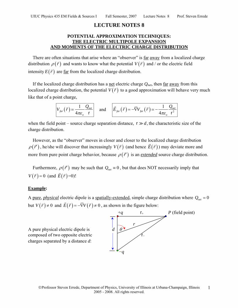
There are often situations that arise where an “observer” is far away from a localized charge distribution ( )rρ and wants to know what the potential ( )V r and / or the electric field

intensity ( )E r are far from the localized charge distribution. If the localized charge distribution has a net electric charge Qnet, then far away from this localized charge distribution, the potential ( )V r to a good approximation will behave very much like that of a point charge,

( ) 14

netfar

o

QV rπε r

and ( ) ( ) 2

14

netfar far

o

QE r V rπε

= −∇ −r

when the field point – source charge separation distance, ,dr the characteristic size of the charge distribution. However, as the “observer” moves in closer and closer to the localized charge distribution ( )rρ ′ , he/she will discover that increasingly ( )V r (and hence ( )E r ) may deviate more and

more from pure point charge behavior, because ( )rρ ′ is an extended source charge distribution. Furthermore, ( )rρ ′ may be such that 0netQ ≡ , but that does NOT necessarily imply that

( ) 0V r = (and ( )E r =0)! Example:

A pure, physical electric dipole is a spatially-extended, simple charge distribution where 0netQ =

but ( ) 0V r ≠ and ( ) ( ) 0E r V r= −∇ ≠ , as shown in the figure below: +q r+ P (field point) r A pure physical electric dipole is d θ composed of two opposite electric r− charges separated by a distance d: −q



2

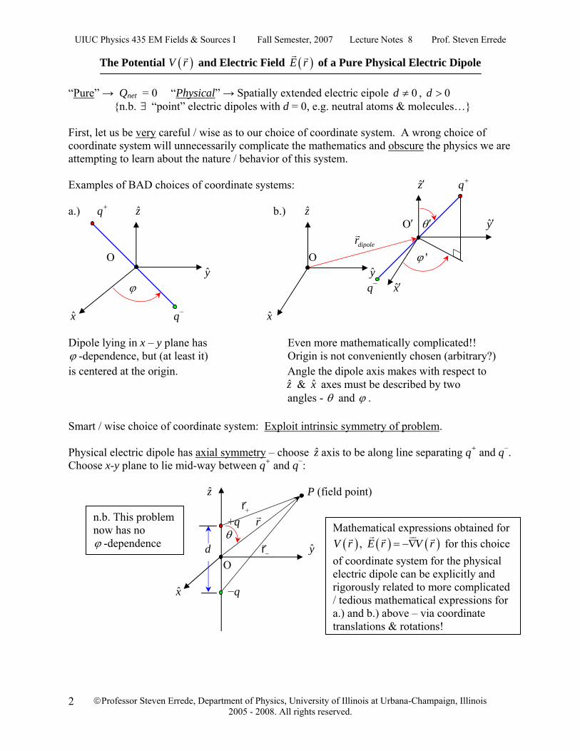
The Potential ( )V r and Electric Field ( )E r of a Pure Physical Electric Dipole “Pure” → Qnet = 0 “Physical” → Spatially extended electric eipole 0d ≠ , 0d > {n.b. ∃ “point” electric dipoles with d = 0, e.g. neutral atoms & molecules…} First, let us be very careful / wise as to our choice of coordinate system. A wrong choice of coordinate system will unnecessarily complicate the mathematics and obscure the physics we are attempting to learn about the nature / behavior of this system. Examples of BAD choices of coordinate systems: z′ q+ a.) q+ z b.) z ′Ο θ ′ y′ dipoler Ο Ο 'ϕ y y ϕ q− x′ x q− x Dipole lying in x – y plane has Even more mathematically complicated!! ϕ -dependence, but (at least it) Origin is not conveniently chosen (arbitrary?) is centered at the origin. Angle the dipole axis makes with respect to z & x axes must be described by two angles - θ and ϕ . Smart / wise choice of coordinate system: Exploit intrinsic symmetry of problem. Physical electric dipole has axial symmetry – choose z axis to be along line separating q+ and q−. Choose x-y plane to lie mid-way between q+ and q−: z P (field point) +r +q r θ d −r

y Ο x −q

Mathematical expressions obtained for ( ) ( ) ( ), V r E r V r= −∇ for this choice

of coordinate system for the physical electric dipole can be explicitly and rigorously related to more complicated / tedious mathematical expressions for a.) and b.) above – via coordinate translations & rotations!

n.b. This problem now has no ϕ -dependence



3

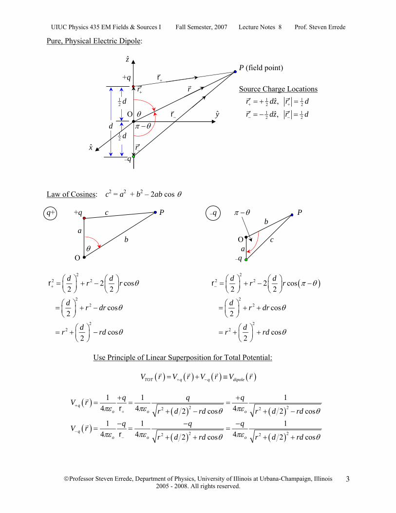
Pure, Physical Electric Dipole: z P (field point) +q +r r+′ r Source Charge Locations 1

2 d 1 12 2ˆ, r dz r d+ +′ ′= + =

Ο θ −r y 1 12 2ˆ, r dz r d− −′ ′= − =

d π θ− 1

2 d x r−′ −q Law of Cosines: c2 = a2 + b2 – 2ab cos θ q+ +q c P −q π θ− P b

a b Ο c θ a

Ο −q

22 2

22

22

2 cos2 2

cos2

cos2

d dr r

d r dr

dr rd

θ

θ

θ

+⎛ ⎞ ⎛ ⎞= + −⎜ ⎟ ⎜ ⎟⎝ ⎠ ⎝ ⎠

⎛ ⎞= + −⎜ ⎟⎝ ⎠

⎛ ⎞= + −⎜ ⎟⎝ ⎠

r

( )2

2 2

22

22

2 cos2 2

cos2

cos2

d dr r

d r dr

dr rd

π θ

θ

θ

−⎛ ⎞ ⎛ ⎞= + − −⎜ ⎟ ⎜ ⎟⎝ ⎠ ⎝ ⎠

⎛ ⎞= + +⎜ ⎟⎝ ⎠

⎛ ⎞= + +⎜ ⎟⎝ ⎠

r

Use Principle of Linear Superposition for Total Potential:

( ) ( ) ( ) ( )TOT q q dipoleV r V r V r V r+ −= + ≡

( )( ) ( )2 22 2

1 1 14 4 42 cos 2 cos

qo o o

q q qV rr d rd r d rdπε πε πεθ θ

++

+ += = =

+ − + −r

( )( ) ( )2 22 2

1 1 14 4 42 cos 2 cos

qo o o

q q qV rr d rd r d rdπε πε πεθ θ

−−

− − −= = =

+ + + +r



4

( ) ( ) ( )

( ) ( )

( ) ( )

2 22 2

2 22 2

1 1 4 4

1 1 4 42 cos 2 cos

1 1 4 2 cos 2 cos

dipole q qo o

o o

o

q qV r V r V r

q q

r d rd r d rd

q

r d rd r d rd

πε πε

πε πεθ θ

πε θ θ

+ −+ −

+∴ = + = −

= −+ − + +

⎡ ⎤⎢ ⎥= −⎢ ⎥+ − + +⎣ ⎦

r r

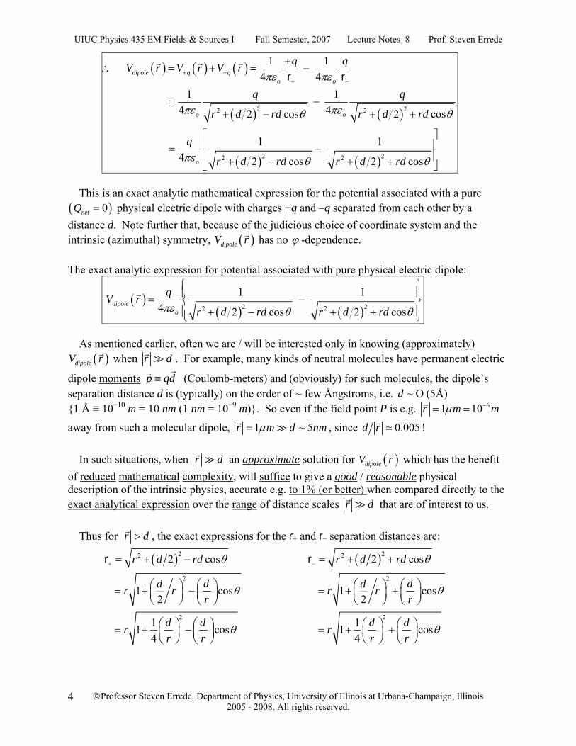
This is an exact analytic mathematical expression for the potential associated with a pure ( )0netQ = physical electric dipole with charges +q and –q separated from each other by a distance d. Note further that, because of the judicious choice of coordinate system and the intrinsic (azimuthal) symmetry, ( )dipoleV r has no ϕ -dependence. The exact analytic expression for potential associated with pure physical electric dipole:

( )( ) ( )2 22 2

1 1 4 2 cos 2 cos

dipoleo

qV rr d rd r d rdπε θ θ

⎧ ⎫⎪ ⎪= −⎨ ⎬⎪ ⎪+ − + +⎩ ⎭

As mentioned earlier, often we are / will be interested only in knowing (approximately)

( )dipoleV r when r d . For example, many kinds of neutral molecules have permanent electric

dipole moments p qd≡ (Coulomb-meters) and (obviously) for such molecules, the dipole’s separation distance d is (typically) on the order of ~ few Ångstroms, i.e. ~d Ο (5Å) {1 Å ≡ 10−10 m = 10 nm (1 nm = 10−9 m)}. So even if the field point P is e.g. 61 10r m mμ −= =

away from such a molecular dipole, 1 ~ 5r m d nmμ= , since 0.005d r ! In such situations, when r d an approximate solution for ( )dipoleV r which has the benefit of reduced mathematical complexity, will suffice to give a good / reasonable physical description of the intrinsic physics, accurate e.g. to 1% (or better) when compared directly to the exact analytical expression over the range of distance scales r d that are of interest to us. Thus for r d> , the exact expressions for the r+ and r− separation distances are:

( )22

2

2

2 cos

1 cos2

1 1 cos4

r d rd

ddr rr

d drr r

θ

θ

θ

+ = + −

⎛ ⎞⎛ ⎞= + −⎜ ⎟ ⎜ ⎟⎝ ⎠ ⎝ ⎠

⎛ ⎞ ⎛ ⎞= + −⎜ ⎟ ⎜ ⎟⎝ ⎠ ⎝ ⎠

r

( )22

2

2

2 cos

1 cos2

1 1 cos4

r d rd

ddr rr

d drr r

θ

θ

θ

− = + +

⎛ ⎞⎛ ⎞= + +⎜ ⎟ ⎜ ⎟⎝ ⎠ ⎝ ⎠

⎛ ⎞ ⎛ ⎞= + +⎜ ⎟ ⎜ ⎟⎝ ⎠ ⎝ ⎠

r



5

Now if ( ) 1d r , then let us define:

21 cos

4d dr r

ε θ+⎛ ⎞ ⎛ ⎞≡ −⎜ ⎟ ⎜ ⎟⎝ ⎠ ⎝ ⎠

and: 21 cos

4d dr r

ε θ−⎛ ⎞ ⎛ ⎞≡ +⎜ ⎟ ⎜ ⎟⎝ ⎠ ⎝ ⎠

Then:

1 11r ε+ +

=+r

and:

1 11r ε− −

=+r

with: 1ε+ and: 1ε−

Now if 1ε+ and 1ε− , we can use the Binomial Expansion (a specific version of the more generalized Taylor Series Expansion) of the expression:

( )1 2 321 1 1 3 1 3 51 1 ... ...

2 2 4 2 4 61ε ε ε ε

ε−

± ± ± ±±

= + = − + − + −+

i i ii i i

(Valid on the interval: 1 1ε±− ≤ ≤ + )

Since ε± is already <<1, then the higher-order terms ( ) ( ) ( )2 3 4, , ,...ε ε ε± ± ± etc. are incredibly small (<<<<<1), so negligible error is incurred by neglecting these higher-order terms,

i.e. keeping only terms linear in ε± in the binomial expansion of 11 ε±+

, we have:

( )12

1 1 1 11 rr

εε +

+ +

= −+r

and: ( )12

1 1 1 11 rr

εε −

− −

= −+r

Then: ( ) ( ) ( )1 1

2 2

1 1 1 11 14 4

1 14

dipole

o o

o

q qV rr r

qx

ε επε πε

πε

+ −+ −

⎧ ⎫ ⎧ ⎫= − − − −⎨ ⎬ ⎨ ⎬⎩ ⎭⎩ ⎭

⎛ ⎞= ⎜ ⎟⎝ ⎠

r r

12 1ε+− −{ } ( )( ){ }1 1

2 21

4 o

qr

ε ε επε− − +

⎛ ⎞+ = −⎜ ⎟⎝ ⎠

Now: 21 cos

4d dr r

ε θ+⎛ ⎞ ⎛ ⎞≡ −⎜ ⎟ ⎜ ⎟⎝ ⎠ ⎝ ⎠

and: 21 cos

4d dr r

ε θ−⎛ ⎞ ⎛ ⎞≡ +⎜ ⎟ ⎜ ⎟⎝ ⎠ ⎝ ⎠

Then:

( )21 1 1

4 2 4dipoleo

q dV rr rπε

⎛ ⎞ ⎛ ⎞ ⎛ ⎞⎛ ⎞= ⎜ ⎟ ⎜ ⎟ ⎜ ⎟⎜ ⎟⎝ ⎠ ⎝ ⎠ ⎝ ⎠⎝ ⎠

21cos 4

d dr r

θ⎛ ⎞⎛ ⎞ ⎛ ⎞⎛ ⎞⎜ ⎟+ −⎜ ⎟ ⎜ ⎟⎜ ⎟⎜ ⎟⎝ ⎠ ⎝ ⎠⎝ ⎠⎝ ⎠

cos

1 1 cos cos4 2

1 1 4 2

o

o

dr

q d dr r r

qr

θ

θ θπε

πε

⎧ ⎫⎡ ⎤⎛ ⎞⎪ ⎪⎛ ⎞⎢ ⎥⎜ ⎟−⎨ ⎬⎜ ⎟⎜ ⎟⎢ ⎥⎝ ⎠⎪ ⎪⎝ ⎠⎣ ⎦⎩ ⎭⎧ ⎫⎛ ⎞⎛ ⎞ ⎛ ⎞ ⎛ ⎞= +⎨ ⎬⎜ ⎟⎜ ⎟ ⎜ ⎟ ⎜ ⎟

⎝ ⎠⎝ ⎠ ⎝ ⎠ ⎝ ⎠⎩ ⎭

⎛ ⎞= ⎜ ⎟⎝ ⎠

2⎛ ⎞⎜ ⎟⎝ ⎠

1cos cos4 o

d q dr r r

θ θπε

⎧ ⎫⎛ ⎞ ⎛ ⎞⎛ ⎞=⎨ ⎬⎜ ⎟ ⎜ ⎟⎜ ⎟⎝ ⎠ ⎝ ⎠⎝ ⎠⎩ ⎭

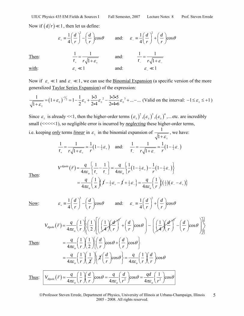
Thus: ( ) 2 2

1 1 cos cos cos4 4 4dipole

o o o

q d q d qdV rr r r r

θ θ θπε πε πε

⎛ ⎞⎛ ⎞ ⎛ ⎞ ⎛ ⎞= =⎜ ⎟⎜ ⎟ ⎜ ⎟ ⎜ ⎟⎝ ⎠⎝ ⎠ ⎝ ⎠ ⎝ ⎠



6

The Magnitude of the Electric Dipole Moment: p qd p≡ = Thus, we may also express the potential of a pure physical dipole as:

( ) 2 2

1 1 cos cos4 4dipole

o o

qd pV rr r

θ θπε πε

⎛ ⎞ ⎛ ⎞= =⎜ ⎟ ⎜ ⎟⎝ ⎠ ⎝ ⎠

(valid for d << r)

Note that: ( ) 2

1 dipoleV rr

∼ whereas ( ) 1monopoleV r

r∼ (valid for point charge q located at origin)

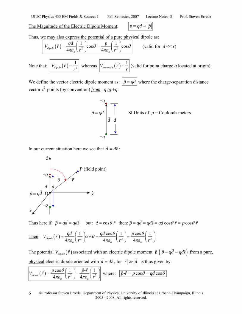
We define the vector electric dipole moment as: p qd≡ where the charge-separation distance vector d points (by convention) from –q to +q: +q p qd≡ SI Units of p = Coulomb-meters d d −q In our current situation here we see that ˆd dz= :

z P (field point)

+q θ r

d d p qd≡ Ο y

−q x Thus here if: ˆp qd qdz= = but: ˆˆ cos z rθ= then: ˆ ˆˆ cos cos p qd qdz qd r p rθ θ= = = =

Then: ( ) 2 2 2

1 cos 1 cos 1cos4 4 4dipole

o o o

qd qd pV rr r r

θ θθπε πε πε

⎛ ⎞ ⎛ ⎞ ⎛ ⎞= =⎜ ⎟ ⎜ ⎟ ⎜ ⎟⎝ ⎠ ⎝ ⎠ ⎝ ⎠

The potential ( )dipoleV r associated with an electric dipole moment p ( )ˆp qd qdz= = from a pure,

physical electric dipole oriented with ˆd dz= , for r d is thus given by:

( ) 2 2

ˆcos 1 14 4dipole

o o

p p rV rr r

θπε πε

⎛ ⎞ ⎛ ⎞=⎜ ⎟ ⎜ ⎟⎝ ⎠ ⎝ ⎠

i where: ˆ cos cosp r p qdθ θ= =i



7

The electric field ( )dipoleE r associated with a pure, physical electric dipole,

with electric dipole moment ˆp qd qdz= = is:

( ) ( ) ( ) ( ) ( )ˆ ˆˆdipole dipole dipoledipole dipole rE r V r E r r E r E rθ ϕθ ϕ= −∇ = + + in spherical-polar coordinates.

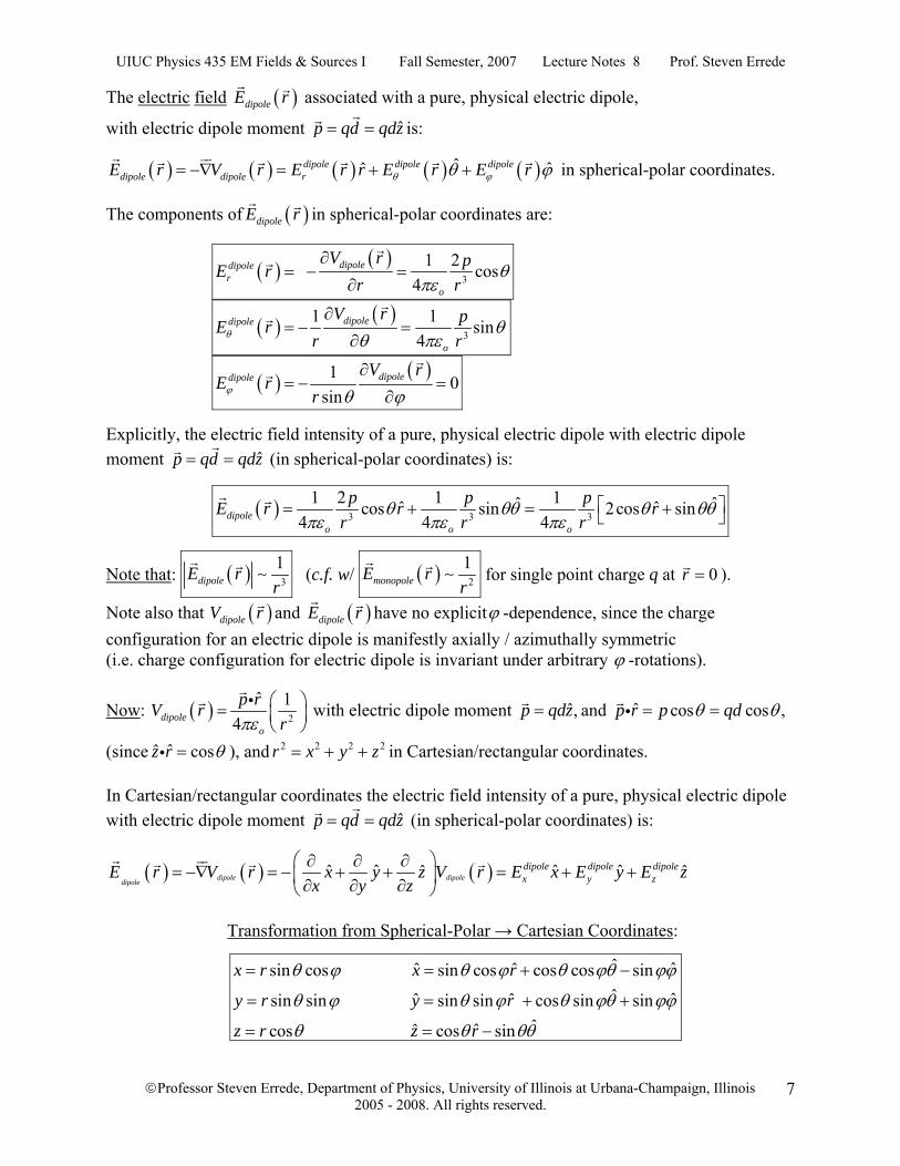
The components of ( )dipoleE r in spherical-polar coordinates are:

( ) ( )3

1 2 cos4

dipoledipoler

o

V r pE rr r

θπε

∂= − =

∂

( ) ( )3

1 1 sin4

dipoledipole

o

V r pE rr rθ θ

θ πε∂

= − =∂

( ) ( )1 0sin

dipoledipole V rE r

rϕ θ ϕ∂

= − =∂

Explicitly, the electric field intensity of a pure, physical electric dipole with electric dipole moment ˆp qd qdz= = (in spherical-polar coordinates) is:

( ) 3 3 3

1 2 1 1ˆ ˆˆ ˆcos sin 2cos sin4 4 4dipole

o o o

p p pE r r rr r r

θ θθ θ θθπε πε πε

⎡ ⎤= + = +⎣ ⎦

Note that: ( ) 3

1dipoleE r

r∼ (c.f. w/ ( ) 2

1monopoleE r

r∼ for single point charge q at 0r = ).

Note also that ( )dipoleV r and ( )dipoleE r have no explicitϕ -dependence, since the charge configuration for an electric dipole is manifestly axially / azimuthally symmetric (i.e. charge configuration for electric dipole is invariant under arbitrary ϕ -rotations).

Now: ( ) 2

ˆ 14dipole

o

p rV rrπε

⎛ ⎞= ⎜ ⎟⎝ ⎠

i with electric dipole moment ˆ,p qdz= and ˆ cos cos ,p r p qdθ θ= =i

(since ˆˆ cosz r θ=i ), and 2 2 2 2r x y z= + + in Cartesian/rectangular coordinates. In Cartesian/rectangular coordinates the electric field intensity of a pure, physical electric dipole with electric dipole moment ˆp qd qdz= = (in spherical-polar coordinates) is:

( ) ( ) ( )ˆ ˆ ˆ ˆˆ ˆdipole dipoledipole

dipole dipole dipolex y zE r V r x y z V r E x E y E z

x y z⎛ ⎞∂ ∂ ∂

= −∇ = − + + = + +⎜ ⎟∂ ∂ ∂⎝ ⎠

Transformation from Spherical-Polar → Cartesian Coordinates:

ˆ ˆˆ ˆsin cos sin cos cos cos sinˆ ˆˆ ˆsin sin sin sin cos sin sin

ˆˆˆcos cos sin

x r x r

y r y r

z r z r

θ ϕ θ ϕ θ ϕθ ϕϕ

θ ϕ θ ϕ θ ϕθ ϕϕ

θ θ θθ

= = + −

= = + +

= = −



8

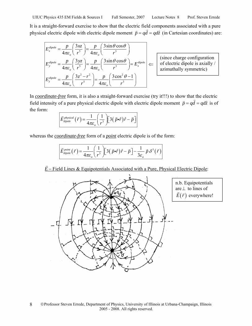
It is a straight-forward exercise to show that the electric field components associated with a pure physical electric dipole with electric dipole moment ˆp qd qdz= = (in Cartesian coordinates) are:

5 3

5 3

2 2 2

5 3

3 3sin cos4 4

3 3sin cos4 4

3 3cos 14 4

dipolex

o o

dipole dipoley x

o o

dipolez

o o

p xz pEr r

p yz pE Er r

p z r pEr r

θ θπε πε

θ θπε πε

θπε πε

⎛ ⎞ ⎛ ⎞= =⎜ ⎟ ⎜ ⎟⎝ ⎠ ⎝ ⎠

⎛ ⎞ ⎛ ⎞= = =⎜ ⎟ ⎜ ⎟⎝ ⎠ ⎝ ⎠

⎛ ⎞ ⎛ ⎞− −= =⎜ ⎟ ⎜ ⎟

⎝ ⎠ ⎝ ⎠

⇐

In coordinate-free form, it is also a straight-forward exercise (try it!!!) to show that the electric field intensity of a pure physical electric dipole with electric dipole moment ˆp qd qdz= = is of the form:

( ) ( )3

1 1 ˆ ˆ34

physicaldipole

o

E r p r r prπε

⎛ ⎞= −⎡ ⎤⎜ ⎟ ⎣ ⎦⎝ ⎠i

whereas the coordinate-free form of a point electric dipole is of the form:

( ) ( ) ( )33

1 1 1ˆ ˆ3 4 3

pointdipole

o o

E r p r r p p rr

δπε ε

⎛ ⎞= − −⎡ ⎤⎜ ⎟ ⎣ ⎦⎝ ⎠i

E − Field Lines & Equipotentials Associated with a Pure, Physical Electric Dipole:

(since charge configuration of electric dipole is axially / azimuthally symmetric)

n.b. Equipotentials are⊥ to lines of ( )E r everywhere!



9

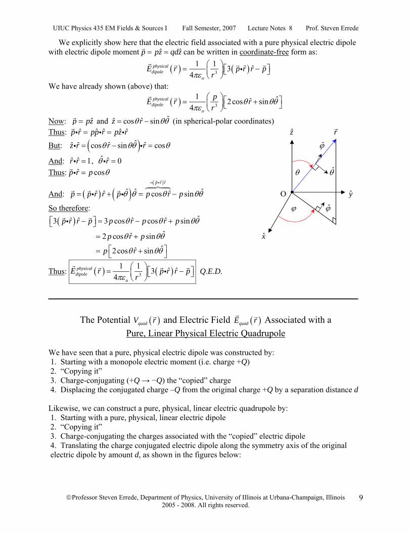
We explicitly show here that the electric field associated with a pure physical electric dipole with electric dipole moment ˆ ˆp pz qdz= = can be written in coordinate-free form as:

( ) ( )3

1 1 ˆ ˆ34

physicaldipole

o

E r p r r prπε

⎛ ⎞= −⎡ ⎤⎜ ⎟ ⎣ ⎦⎝ ⎠i

We have already shown (above) that:

( ) 3

1 ˆˆ2cos sin4

physicaldipole

o

pE r rr

θ θθπε

⎛ ⎞ ⎡ ⎤= +⎜ ⎟ ⎣ ⎦⎝ ⎠

Now: ˆp pz= and ˆˆˆ cos sinz rθ θθ= − (in spherical-polar coordinates) Thus: ˆ ˆ ˆ ˆˆp r pp r pz r= =i i i z r

But: ( )ˆˆ ˆ ˆˆ cos sin cosz r r rθ θθ θ= − =i i ϕ

And: ˆ ˆ 1r r =i , ˆ ˆ 0rθ =i Thus: ˆ cosp r p θ=i θ θ

And: ( ) ( )( )ˆ ˆ

ˆ ˆ ˆˆ ˆ ˆcos sinp r r

p p r r p p r pθ θ θ θθ=

= + = −

i

i i O y

So therefore: ϕ ϕ

( ) ˆˆ ˆ ˆ ˆ3 3 cos cos sinˆˆ 2 cos sinˆˆ 2cos sin

p r r p p r p r p

p r p

p r

θ θ θθ

θ θθ

θ θθ

− = − +⎡ ⎤⎣ ⎦

= +

⎡ ⎤= +⎣ ⎦

i

x

Thus: ( ) ( )3

1 1 ˆ ˆ34

physicaldipole

o

E r p r r prπε

⎛ ⎞= −⎡ ⎤⎜ ⎟ ⎣ ⎦⎝ ⎠i Q.E.D.

The Potential ( )quadV r and Electric Field ( )quadE r Associated with a

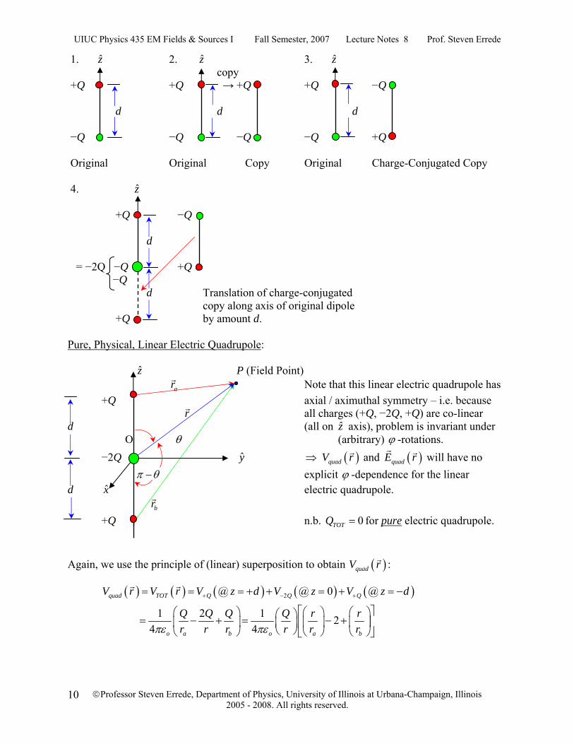
Pure, Linear Physical Electric Quadrupole We have seen that a pure, physical electric dipole was constructed by: 1. Starting with a monopole electric moment (i.e. charge +Q) 2. “Copying it” 3. Charge-conjugating (+Q → −Q) the “copied” charge 4. Displacing the conjugated charge –Q from the original charge +Q by a separation distance d Likewise, we can construct a pure, physical, linear electric quadrupole by: 1. Starting with a pure, physical, linear electric dipole 2. “Copying it” 3. Charge-conjugating the charges associated with the “copied” electric dipole 4. Translating the charge conjugated electric dipole along the symmetry axis of the original electric dipole by amount d, as shown in the figures below:



10

1. z 2. z 3. z copy +Q +Q → +Q +Q −Q d d d −Q −Q −Q −Q +Q Original Original Copy Original Charge-Conjugated Copy 4. z

+Q −Q d = −2Q −Q +Q −Q d Translation of charge-conjugated copy along axis of original dipole +Q by amount d. Pure, Physical, Linear Electric Quadrupole:

z P (Field Point) ar Note that this linear electric quadrupole has +Q axial / aximuthal symmetry – i.e. because r all charges (+Q, −2Q, +Q) are co-linear d (all on z axis), problem is invariant under Ο θ (arbitrary) ϕ -rotations. −2Q y ⇒ ( )quadV r and ( )quadE r will have no π θ− explicit ϕ -dependence for the linear d x electric quadrupole. br +Q n.b. 0TOTQ = for pure electric quadrupole. Again, we use the principle of (linear) superposition to obtain ( )quadV r :

( ) ( ) ( ) ( ) ( )2@ @ 0 @

1 2 1 24 4

quad TOT Q Q Q

o a b o a b

V r V r V z d V z V z d

Q Q Q Q r rr r r r r rπε πε

+ − += = = + + = + = −

⎡ ⎤⎛ ⎞ ⎛ ⎞ ⎛ ⎞⎛ ⎞= − + = − +⎢ ⎥⎜ ⎟ ⎜ ⎟ ⎜ ⎟⎜ ⎟⎝ ⎠⎝ ⎠ ⎝ ⎠ ⎝ ⎠⎣ ⎦



11

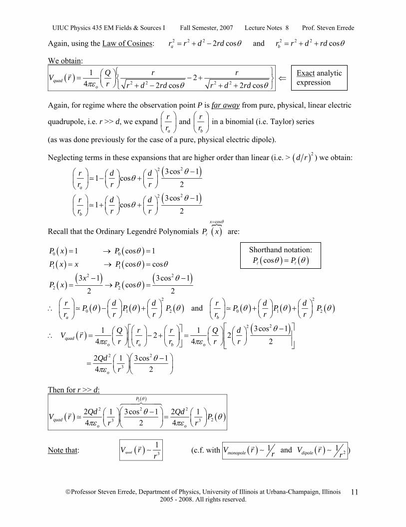
Again, using the Law of Cosines: 2 2 2 2 cosar r d rd θ= + − and 2 2 2 cosbr r d rd θ= + + We obtain:

( )2 2 2 2

1 24 2 cos 2 cos

quado

Q r rV rr r d rd r d rdπε θ θ

⎧ ⎫⎛ ⎞= − +⎨ ⎬⎜ ⎟⎝ ⎠ + − + +⎩ ⎭

⇐

Again, for regime where the observation point P is far away from pure, physical, linear electric

quadrupole, i.e. r >> d, we expand a

rr

⎛ ⎞⎜ ⎟⎝ ⎠

and b

rr

⎛ ⎞⎜ ⎟⎝ ⎠

in a binomial (i.e. Taylor) series

(as was done previously for the case of a pure, physical electric dipole).

Neglecting terms in these expansions that are higher order than linear (i.e. > ( )2d r ) we obtain:

( )22 3cos 1

1 cos2a

r d dr r r

θθ

−⎛ ⎞ ⎛ ⎞ ⎛ ⎞− +⎜ ⎟ ⎜ ⎟ ⎜ ⎟⎝ ⎠ ⎝ ⎠⎝ ⎠

( )22 3cos 1

1 cos2b

r d dr r r

θθ

−⎛ ⎞ ⎛ ⎞ ⎛ ⎞+ +⎜ ⎟ ⎜ ⎟ ⎜ ⎟⎝ ⎠ ⎝ ⎠⎝ ⎠

Recall that the Ordinary Legendré Polynomials ( )cosx

P xθ=

are:

( ) ( )0 01 cos 1P x P θ= → =

( ) ( )1 1 cos cosP x x P θ θ= → =

( ) ( ) ( ) ( )2 2

2 2

3 1 3cos 1cos

2 2x

P x Pθ

θ− −

= → =

( ) ( ) ( )2

0 1 2 a

r d dP P Pr r r

θ θ θ⎛ ⎞ ⎛ ⎞ ⎛ ⎞∴ − +⎜ ⎟ ⎜ ⎟ ⎜ ⎟

⎝ ⎠ ⎝ ⎠⎝ ⎠ and ( ) ( ) ( )

2

0 1 2b

r d dP P Pr r r

θ θ θ⎛ ⎞ ⎛ ⎞ ⎛ ⎞+ +⎜ ⎟ ⎜ ⎟ ⎜ ⎟

⎝ ⎠ ⎝ ⎠⎝ ⎠

( ) ( )22

2 2

3

3cos 11 1 2 24 4 2

2 1 3cos 1 4 2

quado a b o

o

Q r r Q dV rr r r r r

Qdr

θ

πε πε

θπε

⎡ ⎤−⎡ ⎤⎛ ⎞ ⎛ ⎞⎛ ⎞ ⎛ ⎞ ⎛ ⎞⎢ ⎥∴ = − + =⎢ ⎥⎜ ⎟ ⎜ ⎟⎜ ⎟ ⎜ ⎟ ⎜ ⎟⎝ ⎠ ⎝ ⎠ ⎝ ⎠⎢ ⎥⎝ ⎠ ⎝ ⎠⎣ ⎦ ⎣ ⎦

⎛ ⎞−⎛ ⎞= ⎜ ⎟⎜ ⎟⎝ ⎠⎝ ⎠

Then for r >> d:

( )

( )

( )

2

2 2 2

23 3

2 1 3cos 1 2 14 2 4

P

quado o

Qd QdV r Pr r

θ

θ θπε πε

⎛ ⎞−⎛ ⎞ ⎛ ⎞=⎜ ⎟⎜ ⎟ ⎜ ⎟⎝ ⎠ ⎝ ⎠⎝ ⎠

Note that: ( ) 3

1quadV r

r∼ (c.f. with ( ) ( ) 2

1 1 and monopole dipoleV r V rr r∼ ∼ )

Exact analytic expression

Shorthand notation: ( ) ( )cosP Pθ θ=



12

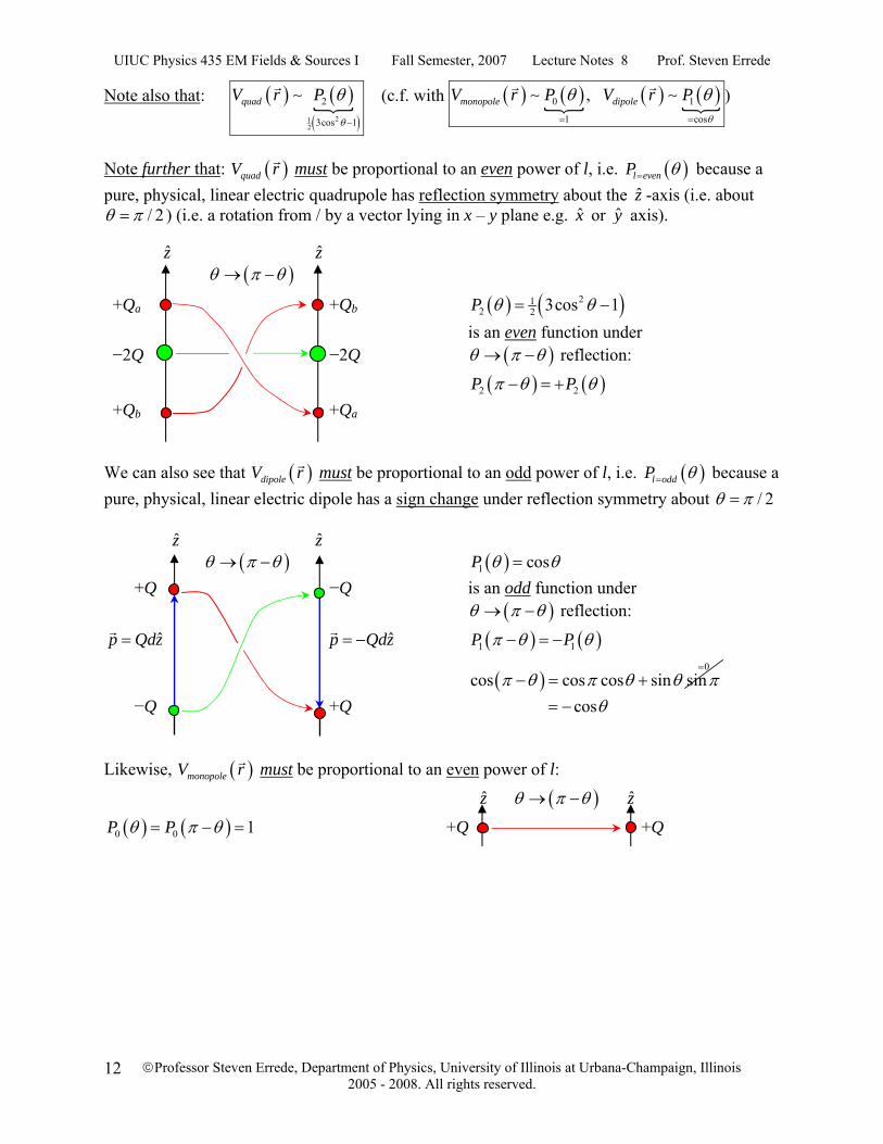
Note also that: ( ) ( )( )21

2

2

3cos 1

quadV r Pθ

θ−

∼ (c.f. with ( ) ( ) ( ) ( )0 1

1 cos

, monopole dipoleV r P V r Pθ

θ θ= =

∼ ∼ )

Note further that: ( )quadV r must be proportional to an even power of l, i.e. ( )l evenP θ= because a pure, physical, linear electric quadrupole has reflection symmetry about the z -axis (i.e. about

/ 2θ π= ) (i.e. a rotation from / by a vector lying in x – y plane e.g. x or y axis).

z z ( )θ π θ→ −

+Qa +Qb ( ) ( )212 2 3cos 1P θ θ= −

is an even function under −2Q −2Q ( )θ π θ→ − reflection:

( ) ( )2 2P Pπ θ θ− = + +Qb +Qa We can also see that ( )dipoleV r must be proportional to an odd power of l, i.e. ( )l oddP θ= because a pure, physical, linear electric dipole has a sign change under reflection symmetry about / 2θ π=

z z ( )θ π θ→ − ( )1 cosP θ θ=

+Q −Q is an odd function under ( )θ π θ→ − reflection:

ˆp Qdz= ˆp Qdz= − ( ) ( )1 1P Pπ θ θ− = −

( )0

cos cos cos sin sinπ θ π θ θ π=

− = + −Q +Q cosθ= − Likewise, ( )monopoleV r must be proportional to an even power of l:

z ( )θ π θ→ − z

( ) ( )0 0 1P Pθ π θ= − = +Q +Q



13

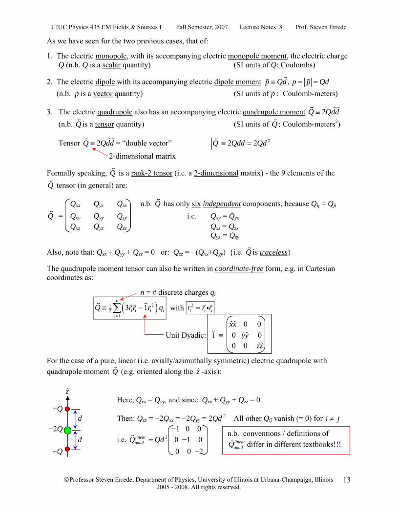
As we have seen for the two previous cases, that of: 1. The electric monopole, with its accompanying electric monopole moment, the electric charge

Q (n.b. Q is a scalar quantity) (SI units of Q: Coulombs)

2. The electric dipole with its accompanying electric dipole moment , p Qd p p Qd≡ = = (n.b. p is a vector quantity) (SI units of p : Coulomb-meters)

3. The electric quadrupole also has an accompanying electric quadrupole moment 2Q Qdd≡ (n.b. Q is a tensor quantity) (SI units of Q : Coulomb-meters2)

Tensor 2Q Qdd≡ = “double vector” 22 2Q Qdd Qd≡ =

2-dimensional matrix

Formally speaking, Q is a rank-2 tensor (i.e. a 2-dimensional matrix) - the 9 elements of the Q tensor (in general) are:

Qxx Qyz Qzx n.b. Q has only six independent components, because Qij = Qji Q = Qxy Qyy Qzy i.e. Qxy = Qyx Qxz Qyz Qzz Qxz = Qzx Qyz = Qzy

Also, note that: Qxx + Qyy + Qzz = 0 or: Qzz = −(Qxx+Qyy) {i.e. Q is traceless} The quadrupole moment tensor can also be written in coordinate-free form, e.g. in Cartesian coordinates as: n = # discrete charges qi

( )212

13 1

n

i i i ii

Q rr r q=

≡ −∑ with 2i i ir r r= i

ˆ ˆxx 0 0 Unit Dyadic: 1 ≡ 0 ˆ ˆyy 0 0 0 ˆˆzz For the case of a pure, linear (i.e. axially/azimuthally symmetric) electric quadrupole with quadrupole moment Q (e.g. oriented along the z -axis): z Here, Qxx = Qyy, and since: Qxx + Qyy + Qzz = 0 +Q d Then: Qzz = −2Qxx = −2Qyy ≡ 2Qd 2 All other Qij vanish (= 0) for i j≠ −2Q −1 0 0 d i.e. 2linear

quadQ Qd= 0 −1 0 +Q 0 0 +2

n.b. conventions / definitions of linearquadQ differ in different textbooks!!!



14

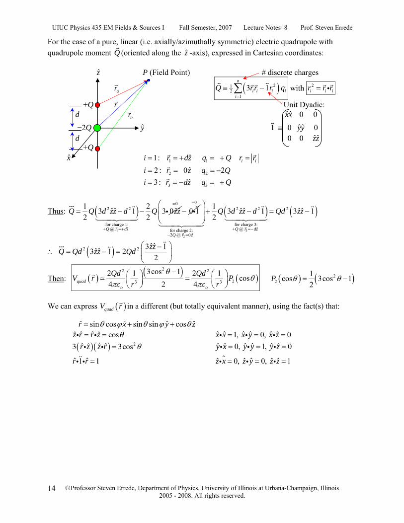
For the case of a pure, linear (i.e. axially/azimuthally symmetric) electric quadrupole with quadrupole moment Q (oriented along the z -axis), expressed in Cartesian coordinates: z P (Field Point) # discrete charges

ar ( )212

13 1

n

i i i ii

Q rr r q=

≡ −∑ with 2i i ir r r= i

+Q r Unit Dyadic: d br ˆ ˆxx 0 0

−2Q y 1 ≡ 0 ˆ ˆyy 0 d 0 0 ˆˆzz +Q x 1 ˆ1: i r dz= = + 1 q Q= + i ir r=

2 ˆ2 : 0i r z= = 2 2q Q= −

3 ˆ3 : i r dz= = − 3 q Q= +

Thus: ( )1

2 2

for charge 1: ˆ+ @

1 2ˆˆ ˆˆ3 1 3 02 2

Q r dz

Q Q d zz d Q zz

=+

= − − i0

0 1=

− i ( ) ( )3

2

02 2 2

for charge 3: ˆ+ @ for charge 2:

ˆ2 @ 0

1 ˆˆ ˆˆ3 1 3 12

Q r dzQ r z

Q d zz d Qd zz=

=−− =

⎛ ⎞+ − = −⎜ ⎟⎜ ⎟

⎝ ⎠

( )2 2 ˆˆ3 1ˆˆ 3 1 22

zzQ Qd zz Qd⎛ ⎞−

∴ = − = ⎜ ⎟⎝ ⎠

Then: ( ) ( ) ( )22 2

23 3

3cos 12 1 2 1 cos4 2 4quad

o o

Qd QdV r Pr r

θθ

πε πε

−⎛ ⎞ ⎛ ⎞=⎜ ⎟ ⎜ ⎟⎝ ⎠ ⎝ ⎠

( ) ( )22

1cos 3cos 12

P θ θ= −

We can express ( )quadV r in a different (but totally equivalent manner), using the fact(s) that: ˆ ˆ ˆ ˆsin cos sin sin cosr x y zθ ϕ θ ϕ θ= + +

ˆ ˆˆ ˆ cosz r r z θ= =i i ˆ ˆ ˆ ˆ ˆ ˆ1, 0, 0x x x y x z= = =i i i ( )( ) 2ˆ ˆˆ ˆ3 3cosr z z r θ=i i ˆ ˆ ˆ ˆ ˆ ˆ0, 1, 0y x y y y z= = =i i i

ˆ ˆ1 1r r =i i ˆˆ ˆ ˆ ˆ0, 0, 1z x z y z z= = =i i i



15

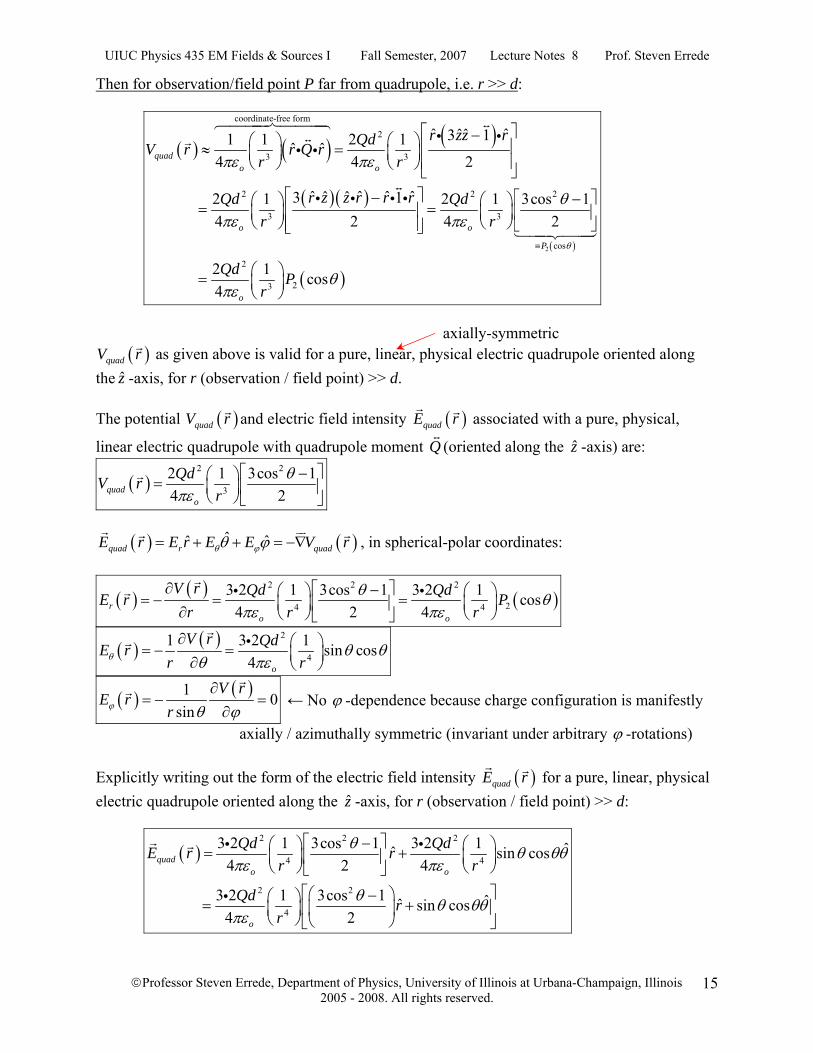
Then for observation/field point P far from quadrupole, i.e. r >> d:

( ) ( ) ( )

( )( )

( )2

coordinate-free form

2

3 3

2 2 2

3 3

cos

ˆ ˆˆˆ3 11 1 2 1ˆ ˆ4 4 2

ˆ ˆ ˆ ˆˆ ˆ3 12 1 2 1 3cos 1 4 2 4 2

quado o

o o

P

r zz rQdV r r Q rr r

r z z r r rQd Qdr r

θ

πε πε

θπε πε

≡

⎡ ⎤−⎛ ⎞ ⎛ ⎞ ⎢ ⎥≈ =⎜ ⎟ ⎜ ⎟ ⎢ ⎥⎝ ⎠ ⎝ ⎠ ⎣ ⎦⎡ ⎤− ⎡ ⎤−⎛ ⎞ ⎛ ⎞= =⎢ ⎥⎜ ⎟ ⎜ ⎟ ⎢ ⎥

⎝ ⎠ ⎝ ⎠⎢ ⎥ ⎣ ⎦⎣ ⎦

i ii i

i i i i

( )2

23

2 1 cos4 o

Qd Pr

θπε

⎛ ⎞= ⎜ ⎟⎝ ⎠

axially-symmetric

( )quadV r as given above is valid for a pure, linear, physical electric quadrupole oriented along the z -axis, for r (observation / field point) >> d. The potential ( )quadV r and electric field intensity ( )quadE r associated with a pure, physical,

linear electric quadrupole with quadrupole moment Q (oriented along the z -axis) are:

( )2 2

3

2 1 3cos 14 2quad

o

QdV rr

θπε

⎡ ⎤−⎛ ⎞= ⎜ ⎟ ⎢ ⎥⎝ ⎠ ⎣ ⎦

( ) ( )ˆ ˆˆquad r quadE r E r E E V rθ ϕθ ϕ= + + = −∇ , in spherical-polar coordinates:

( ) ( ) ( )2 2 2

24 4

3 2 1 3cos 1 3 2 1 cos4 2 4r

o o

V r Qd QdE r Pr r r

θ θπε πε

∂ ⎡ ⎤−⎛ ⎞ ⎛ ⎞= − = =⎜ ⎟ ⎜ ⎟⎢ ⎥∂ ⎝ ⎠ ⎝ ⎠⎣ ⎦

i i

( ) ( ) 2

4

1 3 2 1 sin cos4 o

V r QdE rr rθ θ θ

θ πε∂ ⎛ ⎞= − = ⎜ ⎟∂ ⎝ ⎠

i

( ) ( )1 0sin

V rE r

rϕ θ ϕ∂

= − =∂

← No ϕ -dependence because charge configuration is manifestly

axially / azimuthally symmetric (invariant under arbitrary ϕ -rotations) Explicitly writing out the form of the electric field intensity ( )quadE r for a pure, linear, physical electric quadrupole oriented along the z -axis, for r (observation / field point) >> d:

( )

2 2 2

4 4

2 2

4

3 2 1 3cos 1 3 2 1 ˆˆ sin cos4 2 4

3 2 1 3cos 1 ˆˆ sin cos4 2

quado o

o

Qd QdE r rr r

Qd rr

θ θ θθπε πε

θ θ θθπε

⎡ ⎤−⎛ ⎞ ⎛ ⎞= +⎜ ⎟ ⎜ ⎟⎢ ⎥⎝ ⎠ ⎝ ⎠⎣ ⎦⎡ ⎤⎛ ⎞−⎛ ⎞= +⎢ ⎥⎜ ⎟⎜ ⎟

⎝ ⎠ ⎝ ⎠⎣ ⎦

i i

i



16

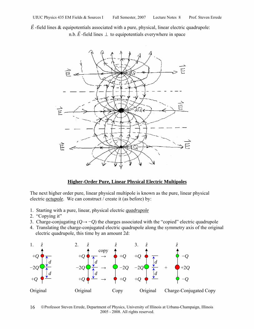
E -field lines & equipotentials associated with a pure, physical, linear electric quadrupole: n.b. E -field lines ⊥ to equipotentials everywhere in space

Higher-Order Pure, Linear Physical Electric Multipoles

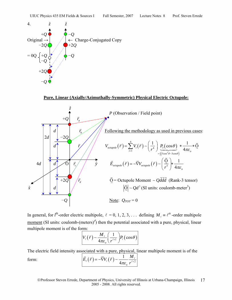
The next higher order pure, linear physical multipole is known as the pure, linear physical electric octupole. We can construct / create it (as before) by: 1. Starting with a pure, linear, physical electric quadrupole 2. “Copying it” 3. Charge-conjugating (Q→ −Q) the charges associated with the “copied” electric quadrupole 4. Translating the charge-conjugated electric quadrupole along the symmetry axis of the original

electric quadrupole, this time by an amount 2d: 1. z 2. z z 3. z z copy +Q +Q → +Q +Q −Q d d d −2Q −2Q → −2Q −2Q + +2Q d d d +Q +Q → +Q +Q −Q Original Original Copy Original Charge-Conjugated Copy



17

4. z z +Q −Q Original → ← Charge-Conjugated Copy −2Q +2Q = 0Q +Q −Q −Q +2Q −Q

Pure, Linear (Axially/Azimuthally-Symmetric) Physical Electric Octupole: z P (Observation / Field point) +Q ar d br Following the methodology as used in previous cases: 2d −2Q

d r ( ) ( ) ( )( )31

2

4

341

5cos 3cos

1 1cos4octupole i

i o

V r V r Pr

θ θ

θπε=

= −

⎛ ⎞= ∗ ∗Ο⎜ ⎟⎝ ⎠

∑ ∼

4d d Ο cr y ( ) ( ) 5

14octupole octupole

o

E r V rr πε

⎛ ⎞Ο= −∇ ∗⎜ ⎟

⎝ ⎠∼

+2Q dr Ο= Octupole Moment Qddd∼ (Rank-3 tensor)

x d 3~ QdΟ (SI units: coulomb-meter3) −Q Note: QTOT = 0

In general, for lth-order electric multipole, = 0, 1, 2, 3, . . . defining thM ≡ -order multipole moment (SI units: coulomb-(meters) ) then the potential associated with a pure, physical, linear multipole moment is of the form:

( ) ( )1

1 cos4 o

MV r Pr

θπε +

⎛ ⎞⎜ ⎟⎝ ⎠

∼

The electric field intensity associated with a pure, physical, linear multipole moment is of the

form: ( ) ( ) 2

14 o

ME r V rrπε += −∇ ∼



18

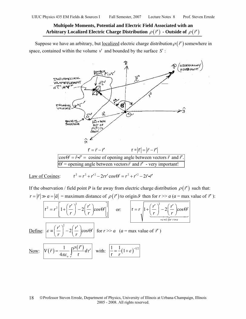
Multipole Moments, Potential and Electric Field Associated with an Arbitrary Localized Electric Charge Distribution ( )rρ ′ - Outside of ( )rρ ′

Suppose we have an arbitrary, but localized electric charge distribution ( )rρ ′ somewhere in space, contained within the volume v′ and bounded by the surface S ′ :

r r′= −r r r′= −r = r ˆ ˆcos cosine of opening angle between vectors and .r r r r′ ′ ′Θ = =i ′Θ = opening angle between vectors and r r′ - very important! Law of Cosines: 2 2 2 22 cos 2r r rr r r r r′ ′ ′ ′ ′= + − Θ = + − i2r If the observation / field point P is far away from electric charge distribution ( )rρ ′ such that:

r r a a= = = maximum distance of ( )rρ ′ to originϑ then for r >> a (a = max value of r′ ): 2

2 1 2 cosr rrr r

⎡ ⎤′ ′⎛ ⎞ ⎛ ⎞ ′= + − Θ⎢ ⎥⎜ ⎟ ⎜ ⎟⎝ ⎠ ⎝ ⎠⎢ ⎥⎣ ⎦

2r or: 2

1

1 2 cos

for r a

r rrr r

ε≡

′ ′⎛ ⎞ ⎛ ⎞ ′= + − Θ⎜ ⎟ ⎜ ⎟⎝ ⎠ ⎝ ⎠

r

Define: 2

2 cosr rr r

ε′ ′⎛ ⎞ ⎛ ⎞ ′≡ − Θ⎜ ⎟ ⎜ ⎟

⎝ ⎠ ⎝ ⎠ for r >> a (a = max value of r′ )

Now: ( ) ( )14 o v

rV r d

ρτ

πε ′

′′= ∫ r with: ( ) 1 21 1 1

rε −= +

r



19

Carry out a (full) binomial expansion of 1/r (for r >> a):

( ) 1/ 2 2 3

0

1 21 1 1 1 1 3 51 1 ... 2 8 16

n

n nr r rε ε ε ε ε

∞−

=

−⎛ ⎞ ⎛ ⎞= + = = − + − +⎜ ⎟ ⎜ ⎟⎝ ⎠⎝ ⎠

∑r

where: ( ) ( )( )

121 2 1

!

n nn n n

− Γ −−⎛ ⎞=⎜ ⎟ Γ⎝ ⎠

is the binomial coefficient and ( )xΓ is the gamma function.

and: ( )( ) ( )( ) ( ) ( )( ) ( )

12 31 1 1 1 1

2 2 2 2 2 21 .... 1 ....n

n nn

Γ −= − − + − + − = − −

Γ

Then: 2 2 3 31 1 1 3 51 2cos 2cos 2cos ...

2 8 16r r r r r r

r r r r r r r⎡ ⎤′ ′ ′ ′ ′ ′⎛ ⎞⎛ ⎞ ⎛ ⎞ ⎛ ⎞ ⎛ ⎞ ⎛ ⎞′ ′ ′= − − Θ + − Θ − − Θ +⎢ ⎥⎜ ⎟⎜ ⎟ ⎜ ⎟ ⎜ ⎟ ⎜ ⎟ ⎜ ⎟

⎝ ⎠⎝ ⎠ ⎝ ⎠ ⎝ ⎠ ⎝ ⎠ ⎝ ⎠⎢ ⎥⎣ ⎦r

Collecting together like powers of r r′ :

32 32 31 1 3cos 1 5cos 3cos1 cos ...

2 2r r r

r r r r

⎡ ⎤′ ′ ′ ′ ′ ′⎛ ⎞ ⎛ ⎞Θ − Θ − Θ⎛ ⎞ ⎛ ⎞ ⎛ ⎞′= + Θ + + +⎢ ⎥⎜ ⎟ ⎜ ⎟⎜ ⎟ ⎜ ⎟ ⎜ ⎟⎝ ⎠ ⎝ ⎠ ⎝ ⎠⎢ ⎥⎝ ⎠ ⎝ ⎠⎣ ⎦r

Thus we see that:

( ) ( ) ( ) ( )2 3

0 1 2 31 1 cos cos cos cos ...r r rP P P P

r r r r⎡ ⎤′ ′ ′⎛ ⎞ ⎛ ⎞ ⎛ ⎞′ ′ ′ ′= Θ + Θ + Θ + Θ +⎢ ⎥⎜ ⎟ ⎜ ⎟ ⎜ ⎟

⎝ ⎠ ⎝ ⎠ ⎝ ⎠⎢ ⎥⎣ ⎦r !!!!

Hence: ( )0

1 1 cosr Pr r

∞

=

′⎛ ⎞ ′= Θ⎜ ⎟⎝ ⎠

∑r where ′Θ = opening angle between and .r r′

This remarkable result occurs because 11 ε+

(where 2

2 cosr rr r

ε′ ′⎛ ⎞ ⎛ ⎞ ′≡ − Θ⎜ ⎟ ⎜ ⎟

⎝ ⎠ ⎝ ⎠) is known as the

Generating Function for the Legendré Polynomials!!!

Then, since ( ) ( )1 14 o v

V r r dr

ρ τπε ′

⎛ ⎞′ ′= ⎜ ⎟⎝ ⎠∫ for r >> a (a = max value of r′ ), the potential outside

the volume v′ containing the charge distribution ( )rρ ′ is given by:

( ) ( ) ( )

( ) ( ) ( )

0

10

1 1 cos4

1 1 cos4

outsideo v

o v

rV r r P dr r

r r P dr

ρ τπε

ρ τπε

∞

=′

∞

+= ′

′⎛ ⎞ ⎛ ⎞ ′ ′ ′= Θ⎜ ⎟ ⎜ ⎟⎝ ⎠ ⎝ ⎠

⎛ ⎞ ′ ′ ′ ′= Θ⎜ ⎟⎝ ⎠

∑∫

∑ ∫

Then defining: ( ) ( ) ( ) ( )1

1 1 cos4

outside

o v

V r r r P dr

ρ τπε +

′

⎛ ⎞ ′ ′ ′ ′= Θ⎜ ⎟⎝ ⎠ ∫



20

We obtain (for r >> a): ( ) ( ) ( ) ( ) ( )10 0

1 1 cos4

outsideoutside

o v

V r V r r r P dr

ρ τπε

∞ ∞

+= = ′

⎛ ⎞ ′ ′ ′ ′= = Θ⎜ ⎟⎝ ⎠

∑ ∑ ∫

Linear superposition of ′Θ = opening angle multipole potentials!!! between and .r r′

This expression is known as the Multipole Expansion of ( )outsideV r in powers of 1/r. It is valid / useful when r >> a (a = max value of r′ ). Note that this is an exact expression.

Having obtained ( )outsideV r , we can then obtain ( ) ( )outside outsideE r V r= −∇ , and thus we see that:

( ) ( ) ( )0 0

outside outsideoutsideE r E r V r

∞ ∞

= =

= = − ∇∑ ∑ i.e. ( ) ( )outside outsideE r V r= −∇

Linear superposition of multipole electric fields!!! Thus, we see that, for observation / field point distances far away from the (arbitrary) localized electric charge distribution ( )rρ ′ (i.e. r >> a (a = max value of r′ )) the electrostatic potential

( )outsideV r and associated electric field ( ) ( )outside outsideE r V r= −∇ are linear superpositions of

multipole electrostatic potentials ( )outsideV r and multipole electric fields ( )outsideE r respectively,

each arising from the th electric multipole moment M associated with the localized electric charge distribution ( )rρ ′ !!!

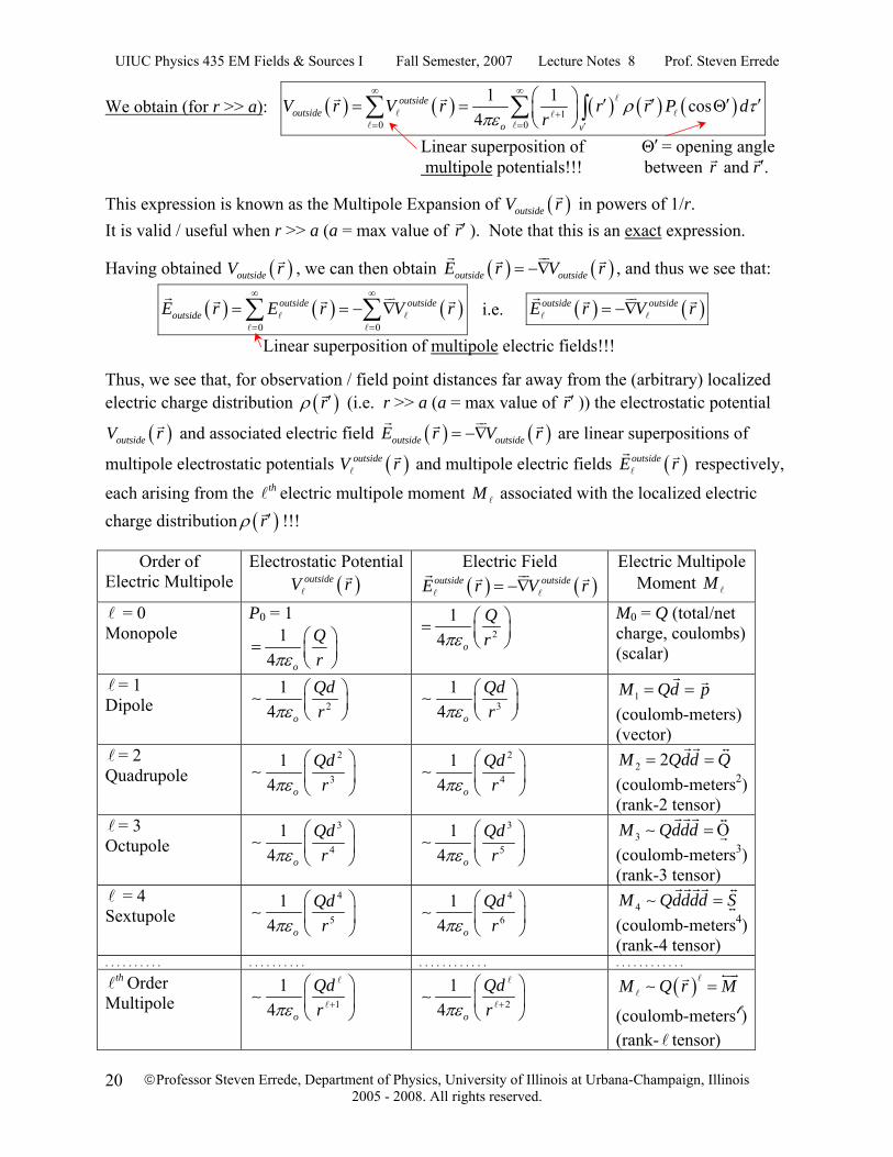
Order of Electric Multipole

Electrostatic Potential( )outsideV r

Electric Field ( ) ( )outside outsideE r V r= −∇

Electric Multipole Moment M

= 0 Monopole

P0 = 1 1

4 o

Qrπε

⎛ ⎞= ⎜ ⎟⎝ ⎠

2

14 o

Qrπε

⎛ ⎞= ⎜ ⎟⎝ ⎠

M0 = Q (total/net charge, coulombs) (scalar)

= 1 Dipole 2

14 o

Qdrπε

⎛ ⎞⎜ ⎟⎝ ⎠

∼ 3

14 o

Qdrπε

⎛ ⎞⎜ ⎟⎝ ⎠

∼ 1M Qd p= = (coulomb-meters) (vector)

= 2 Quadrupole

2

3

14 o

Qdrπε

⎛ ⎞⎜ ⎟⎝ ⎠

∼ 2

4

14 o

Qdrπε

⎛ ⎞⎜ ⎟⎝ ⎠

∼ 2 2M Qdd Q= = (coulomb-meters2)(rank-2 tensor)

= 3 Octupole

3

4

14 o

Qdrπε

⎛ ⎞⎜ ⎟⎝ ⎠

∼ 3

5

14 o

Qdrπε

⎛ ⎞⎜ ⎟⎝ ⎠

∼ 3M Qddd = Ο∼ (coulomb-meters3)(rank-3 tensor)

= 4 Sextupole

4

5

14 o

Qdrπε

⎛ ⎞⎜ ⎟⎝ ⎠

∼ 4

6

14 o

Qdrπε

⎛ ⎞⎜ ⎟⎝ ⎠

∼ 4M Qdddd S=∼ (coulomb-meters4)(rank-4 tensor)

. . . . . . . . . . . . . . . . . . . . . . . . . . . . . . . . . . . . . . . . . . . . th Order

Multipole 1

14 o

Qdrπε +

⎛ ⎞⎜ ⎟⎝ ⎠

∼ 2

14 o

Qdrπε +

⎛ ⎞⎜ ⎟⎝ ⎠

∼ ( )M Q r M=∼

(coulomb-meters ) (rank- tensor)



21

Thus we see that: → The higher-order multipole fields fall off 1/r faster than those associated with next lower

order multipole. → Must get in closer and closer to charge distribution ( )rρ ′ in order to sense / observe / detect

the higher-order moments!

We can write the electrostatic potential yet another way: For r >> a (a = max value of r′ )

( ) ( ) ( ) ( )( )( )

( )2 2

2 30

ˆ31 1 1 1 ....4 2

outsideoutside l

l o v v v

r r rV r V r r d r r r d r d

r r rρ τ ρ τ ρ τ

πε

∞

= ′ ′ ′

⎡ ⎤′ ′−⎢ ⎥′ ′ ′ ′ ′ ′ ′= = + + +⎢ ⎥⎢ ⎥⎣ ⎦

∑ ∫ ∫ ∫i

i

Thus, we see that: ( ) 2 3

ˆ ˆ ˆ1 .....4

Netoutside

omonopole dipole quadrupole

term term term

Q p r r Q rV rr r rπε

⎡ ⎤⎢ ⎥⎢ ⎥= + + +⎢ ⎥⎢ ⎥⎣ ⎦

i i i

with: ( )Netv

Q r dρ τ′

′ ′≡ ∫ , ( )v

p r r dρ τ′

′ ′ ′≡ ∫ and ( )( )

( )2 2ˆ3

2v

r r rQ r dρ τ

′

′ ′−′ ′≡ ∫

i …..

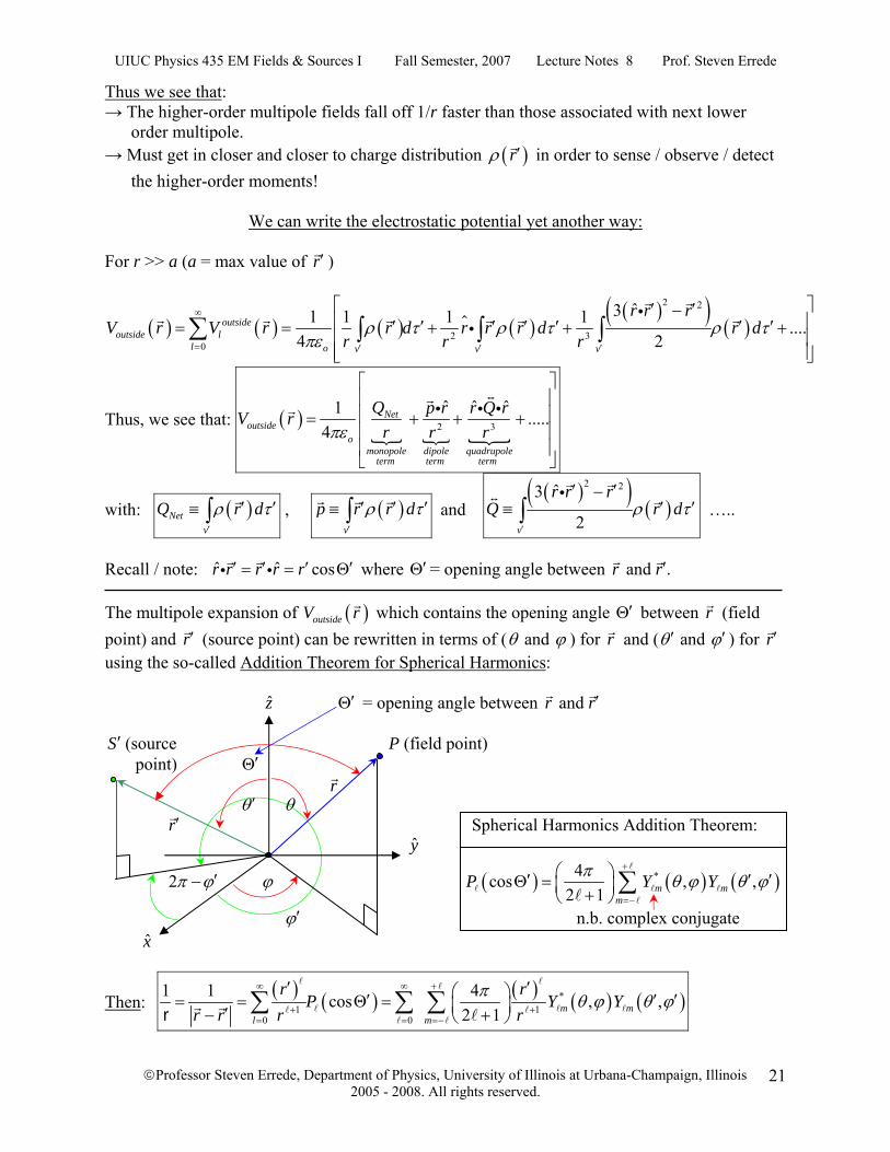
Recall / note: ˆ ˆ cosr r r r r′ ′ ′ ′= = Θi i where ′Θ = opening angle between and .r r′ The multipole expansion of ( )outsideV r which contains the opening angle ′Θ between r (field point) and r′ (source point) can be rewritten in terms of ( and θ ϕ ) for r and ( and θ ϕ′ ′ ) for r′ using the so-called Addition Theorem for Spherical Harmonics: z ′Θ = opening angle between and r r′ S ′ (source P (field point) point) ′Θ r θ ′ θ r′ Spherical Harmonics Addition Theorem: y

2π ϕ′− ϕ ( ) ( ) ( )*4cos , ,2 1 m m

mP Y Yπ θ ϕ θ ϕ

+

=−

⎛ ⎞′ ′ ′Θ = ⎜ ⎟+⎝ ⎠∑

ϕ′ n.b. complex conjugate x

Then: ( ) ( ) ( ) ( ) ( )*

1 10 0

1 1 4cos , ,2 1 m m

l m

r rP Y Y

r r r rπ θ ϕ θ ϕ

∞ ∞ +

+ += = =−

′ ′⎛ ⎞′ ′ ′= = Θ = ⎜ ⎟′− +⎝ ⎠∑ ∑ ∑r



22

Thus:

( ) ( ) ( ) ( )

( ) ( ) ( ) ( )

( )

10

*, ,1

0

0

1 1 cos4

1 1 4 , ,4 2 1

outsideo v

m mmo v

outsidem

m

V r r r P dr

r r Y Y dr l

V r

ρ τπε

π ρ θ ϕ θ ϕ τπε

∞

+= ′

∞ +

+= =−′

∞ +

= =−

⎛ ⎞ ′ ′ ′ ′= Θ⎜ ⎟⎝ ⎠

⎛ ⎞ ⎛ ⎞ ′ ′ ′ ′ ′= ⎜ ⎟ ⎜ ⎟+⎝ ⎠ ⎝ ⎠

=

∑ ∫

∑ ∑∫

∑ ∑

where: ( ) ( ) ( ) ( ) ( )*, ,1

1 4 , ,4 2 1

outsidem m m

o v

rV r r Y Y d

rπ ρ θ ϕ θ ϕ τ

πε +′

′⎛ ⎞ ′ ′ ′ ′= ⎜ ⎟+⎝ ⎠ ∫

Thus:

( ) ( ) ( ) ( ) ( )

( ) ( ) ( ) ( )

*, ,1

0

*, ,1

0

1 4 1 , ,4 2 1

1 4 1 , ,4 2 1

outside m mmo v

m mmo v

V r r r Y Y dl r

Y r r Y dl r

π ρ θ ϕ θ ϕ τπε

π θ ϕ ρ θ ϕ τπε

∞ +

+= =−′

∞ +

+= =− ′

⎛ ⎞⎛ ⎞ ′ ′ ′ ′ ′= ⎜ ⎟⎜ ⎟+⎝ ⎠⎝ ⎠

⎡ ⎤⎛ ⎞⎛ ⎞ ′ ′ ′ ′ ′= ⎢ ⎥⎜ ⎟⎜ ⎟+⎝ ⎠⎝ ⎠ ⎣ ⎦

∑ ∑∫

∑ ∑ ∫

The ( ), ,l mY θ ϕ are the Spherical Harmonics; and θ ϕ are the polar & azimuthal angles for r , the vector from the origin to the field point, P and and θ ϕ′ ′ are the polar & azimuthal angles for r′ , the vector from the origin to the source point, S ′ . We can then define mq - the Electric Multipole Moment of order & m:

( ) ( ) ( ),m mv

q r r Y dρ θ ϕ τ′

′ ′ ′ ′ ′≡ ∫

Because of the properties of the ( ), ,mY θ ϕ , namely that:

( ) ( ) ( )*,, 1 ,m mY Yθ ϕ θ ϕ− = − ( ) ( )( )

( ) ( )2 1 !, cos

4 !im

m

mY P e

mϕθ ϕ θ

π+ −

=+

We see that: ( ) *

,1m mq q− = −

Thus: ( )*, ,1

1 4 1 ,4 2 1

outsidem m m

o

V Y qr

π θ ϕπε +

⎛ ⎞= ⎜ ⎟+⎝ ⎠

Then: ( ) ( ) ( )*, , ,1

0 0

1 4 1 ,4 2 1

outsideoutside m m m

m mo

V r V r Y qr

π θ ϕπε

∞ + ∞ +

+= =− = =−

⎛ ⎞= = ⎜ ⎟+⎝ ⎠∑ ∑ ∑ ∑

Again, ( ) ( )outside outsideE r V r= −∇ which by the principle of linear superposition becomes:

( ) ( ), ,0 0

outside outsidem m

m m

E r V r∞ + ∞ +

= =− = =−

= = − ∇∑ ∑ ∑ ∑

i.e. ( ) ( ), ,

outside outsidem mE r V r= −∇



23

The main advantage of using these seemingly more complex expressions for ( ),outsidemV r

involving the ( )* ,mY θ ϕ and ( ),mY θ ϕ′ ′ spherical harmonics is that they are directly connected to

a right-handed ˆ ˆ ˆx y z− − coordinate system. The earlier expression for ( )outsideV r involving the

( )cosP ′Θ Legendré Polynomials, it must be kept in mind at all times that ′Θ = opening angle between field point r and source point r′ . The explicit derivation of ( )outsideV r using the Addition Theorem for Spherical Harmonics:

( ) ( ) ( ) ( ) ( )*1

0

(electric multipole moment of order & )

1 4 1 , ,4 2 1

m

outside m mmo v

qm

V r Y r r Y dr

π θ ϕ ρ θ ϕ τπε

∞ +

+= =− ′

≡

⎛ ⎞⎛ ⎞ ′ ′ ′ ′ ′= ⎜ ⎟⎜ ⎟+⎝ ⎠⎝ ⎠∑ ∑ ∫

thus makes it explicitly clear that ( ) ( ), ,outsideV r fcn r θ ϕ= only – all source variable

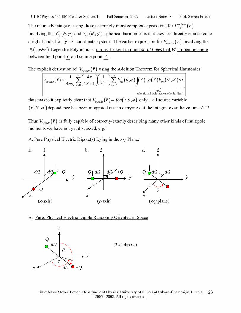
( ), ,r θ ϕ′ ′ ′ dependence has been integrated out, in carrying out the integral over the volume v′ !!! Thus ( )outsideV r is fully capable of correctly/exactly describing many other kinds of multipole moments we have not yet discussed, e.g.: A. Pure Physical Electric Dipole(s) Lying in the x-y Plane: a. z b. z c. z d/2 d/2 −Q −Q d/2 d/2 +Q −Q d/2 d/2 y y y +Q ϕ x x x (x-axis) (y-axis) (x-y plane) B. Pure, Physical Electric Dipole Randomly Oriented in Space: z −Q d/2 (3-D dipole) θ y ϕ x d/2 +Q



24

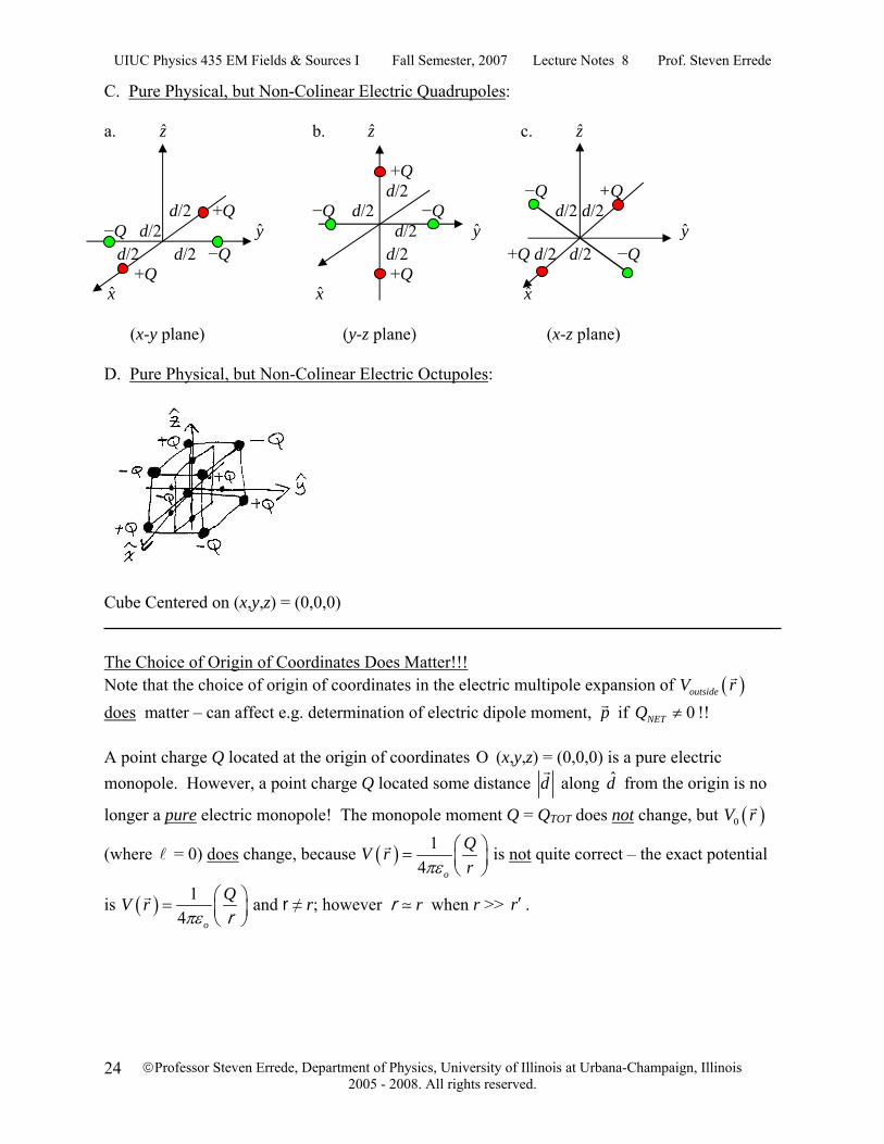
C. Pure Physical, but Non-Colinear Electric Quadrupoles: a. z b. z c. z +Q d/2 −Q +Q d/2 +Q −Q d/2 −Q d/2 d/2 −Q d/2 y d/2 y y d/2 d/2 −Q d/2 +Q d/2 d/2 −Q +Q +Q x x x (x-y plane) (y-z plane) (x-z plane) D. Pure Physical, but Non-Colinear Electric Octupoles:

Cube Centered on (x,y,z) = (0,0,0) The Choice of Origin of Coordinates Does Matter!!! Note that the choice of origin of coordinates in the electric multipole expansion of ( )outsideV r does matter – can affect e.g. determination of electric dipole moment, p if 0NETQ ≠ !! A point charge Q located at the origin of coordinates Ο (x,y,z) = (0,0,0) is a pure electric monopole. However, a point charge Q located some distance d along d from the origin is no

longer a pure electric monopole! The monopole moment Q = QTOT does not change, but ( )0V r

(where = 0) does change, because ( ) 14 o

QV rrπε

⎛ ⎞= ⎜ ⎟⎝ ⎠

is not quite correct – the exact potential

is ( ) 14 o

QV rπε

⎛ ⎞= ⎜ ⎟⎝ ⎠r

and r ≠ r; however rr when r >> r′ .



25

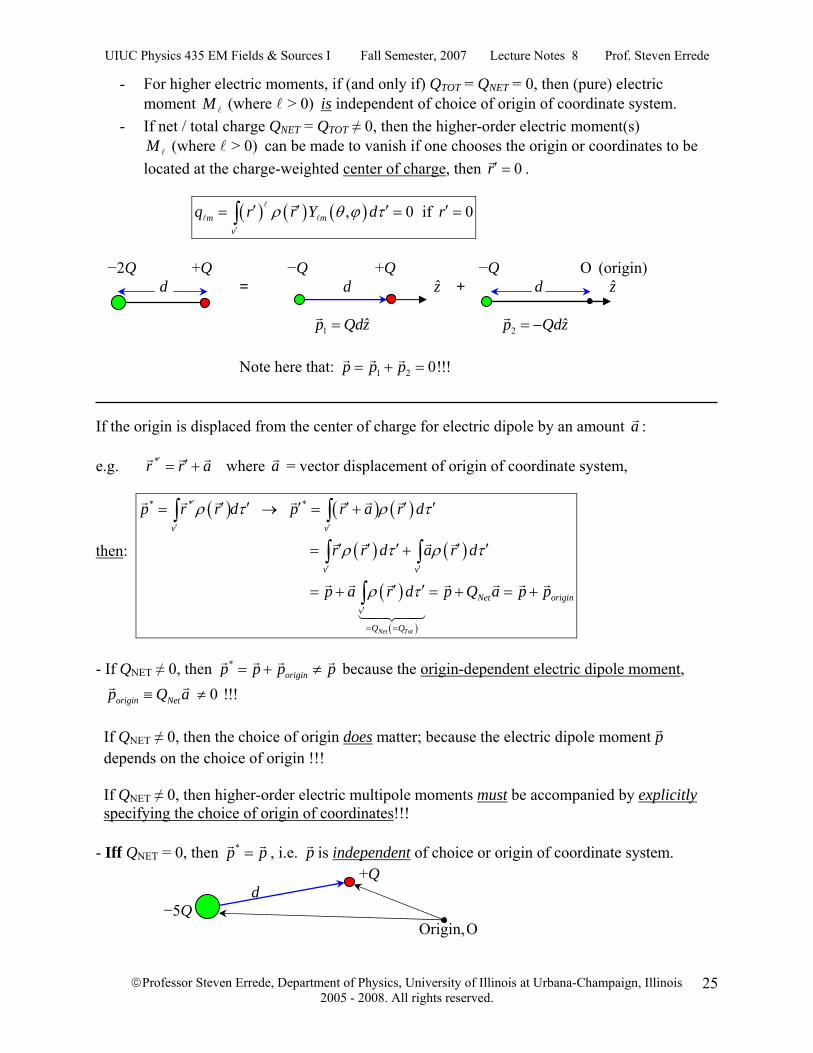
- For higher electric moments, if (and only if) QTOT = QNET = 0, then (pure) electric moment (where > 0)M is independent of choice of origin of coordinate system.

- If net / total charge QNET = QTOT ≠ 0, then the higher-order electric moment(s) (where > 0)M can be made to vanish if one chooses the origin or coordinates to be

located at the charge-weighted center of charge, then 0r′ = .

( ) ( ) ( ), 0 if 0m mv

q r r Y d rρ θ ϕ τ′

′ ′ ′ ′= = =∫

−2Q +Q −Q +Q −Q Ο (origin)

d = d z + d z 1 ˆp Qdz= 2 ˆp Qdz= − Note here that: 1 2 0!!!p p p= + = If the origin is displaced from the center of charge for electric dipole by an amount a : e.g. *r r a′ ′= + where a = vector displacement of origin of coordinate system,

then:

( ) ( ) ( )

( ) ( )

( )

( )

* * *

Net Tot

v v

v v

Netv

Q Q

p r r d p r a r d

r r d a r d

p a r d p Q a

ρ τ ρ τ

ρ τ ρ τ

ρ τ

′

′ ′

′ ′

′

= =

′ ′ ′ ′ ′ ′= → = +

′ ′ ′ ′ ′= +

′ ′= + = +

∫ ∫

∫ ∫

∫ originp p= +

- If QNET ≠ 0, then *

originp p p p= + ≠ because the origin-dependent electric dipole moment, 0 !!!origin Netp Q a≡ ≠ If QNET ≠ 0, then the choice of origin does matter; because the electric dipole moment p depends on the choice of origin !!! If QNET ≠ 0, then higher-order electric multipole moments must be accompanied by explicitly specifying the choice of origin of coordinates!!! - Iff QNET = 0, then *p p= , i.e. p is independent of choice or origin of coordinate system. +Q d −5Q Origin,Ο



26

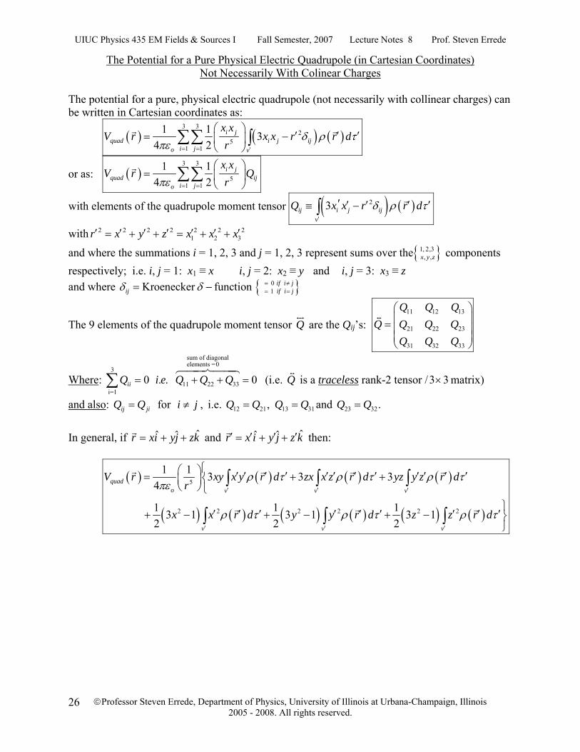
The Potential for a Pure Physical Electric Quadrupole (in Cartesian Coordinates) Not Necessarily With Colinear Charges

The potential for a pure, physical electric quadrupole (not necessarily with collinear charges) can be written in Cartesian coordinates as:

( ) ( ) ( )3 3

25

1 1

1 1 34 2

i jquad i j ij

i jo v

x xV r x x r r d

rδ ρ τ

πε = = ′

⎛ ⎞′ ′ ′= −⎜ ⎟

⎝ ⎠∑∑ ∫

or as: ( )3 3

51 1

1 14 2

i jquad ij

i jo

x xV r Q

rπε = =

⎛ ⎞= ⎜ ⎟

⎝ ⎠∑∑

with elements of the quadrupole moment tensor ( ) ( )23ij i j ijv

Q x x r r dδ ρ τ′

′ ′ ′ ′ ′≡ −∫

with 2 2 2 2 2 2 21 2 3r x y z x x x′ ′ ′ ′ ′ ′ ′= + + = + +

and where the summations i = 1, 2, 3 and j = 1, 2, 3 represent sums over the{ }1, 2,3, ,x y z components

respectively; i.e. i, j = 1: x1 ≡ x i, j = 2: x2 ≡ y and i, j = 3: x3 ≡ z and where { } 0

1 Kroenecker function if i jij if i jδ δ = ≠

= == −

The 9 elements of the quadrupole moment tensor Q are the Qij’s: 11 12 13

21 22 23

31 32 33

Q Q QQ Q Q Q

Q Q Q

⎛ ⎞⎜ ⎟= ⎜ ⎟⎜ ⎟⎝ ⎠

Where:

sum of diagonalelements =0

3

11 22 33i=1

0 . . 0iiQ i e Q Q Q= + + =∑ (i.e. Q is a traceless rank-2 tensor /3 3× matrix)

and also: for ij jiQ Q i j= ≠ , i.e. 12 21,Q Q= 13 31Q Q= and 23 32.Q Q= In general, if ˆˆ ˆr xi yj zk= + + and ˆˆ ˆr x i y j z k′ ′ ′ ′= + + then:

( ) ( ) ( ) ( )

( ) ( ) ( ) ( ) ( ) ( )

5

2 2 2 2 2 2

1 1 3 3 34

1 1 1 3 1 3 1 3 12 2 2

quado v v v

v v v

V r xy x y r d zx x z r d yz y z r dr

x x r d y y r d z z r d

ρ τ ρ τ ρ τπε

ρ τ ρ τ ρ τ

′ ′ ′

′ ′ ′

⎧⎛ ⎞ ′ ′ ′ ′ ′ ′ ′ ′ ′ ′ ′ ′= + +⎨⎜ ⎟⎝ ⎠⎩

⎫′ ′ ′ ′ ′ ′ ′ ′ ′+ − + − + − ⎬

⎭

∫ ∫ ∫

∫ ∫ ∫



27

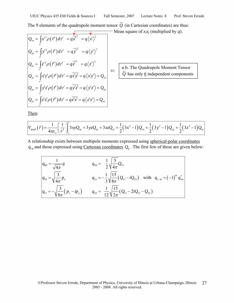
The 9 elements of the quadrupole moment tensor Q (in Cartesian coordinates) are thus: Mean square of xixj (multiplied by q).

( )

( )

( )

( )

( )

( )

2 22

2 22

2 22

xxv

yyv

zzv

xy yxv

yz zyv

zx xv

Q x r d qx q x

Q y r d q y q y

Q z r d qz q z

Q x y r d qx y q x y Q

Q y z r d q y z q y z Q

Q z x r d qz x q z x Q

ρ τ

ρ τ

ρ τ

ρ τ

ρ τ

ρ τ

′

′

′

′

′

′

′ ′ ′ ′ ′= = =

′ ′ ′ ′ ′= = =

′ ′ ′ ′ ′= = =

′ ′ ′ ′ ′ ′ ′ ′= = = =

′ ′ ′ ′ ′ ′ ′ ′= = = =

′ ′ ′ ′ ′ ′ ′ ′= = = =

∫

∫

∫

∫

∫

∫ z

⇐

Then:

( ) ( ) ( ) ( )2 2 25

1 1 1 1 13 3 3 3 1 3 1 3 14 2 2 2quad xy yz xz xx yy zz

o

V r xyQ yzQ xzQ x Q y Q z Qrπε

⎛ ⎞ ⎡= + + + − + − + −⎜ ⎟ ⎢⎝ ⎠ ⎣

A relationship exists between multipole moments expressed using spherical-polar coordinates

mq and those expressed using Cartesian coordinates ijQ . The first few of these are given below:

( ) ( )

( ) ( )

00 20 33

*10 21 13 23

11 22 11 12 22

1 1 5 2 44

3 1 15 with 14 3 8

3 1 15 28 12 2

mz m m

x y

q q q Q

q p q Q iQ q q

q p ip q Q iQ Q

ππ

π π

π π

−

= =

= = − − = −

= − − = − −

n.b. The Quadrupole Moment Tensor Q has only 6 independent components



28

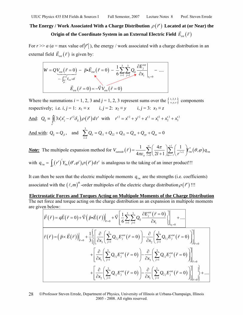
The Energy / Work Associated With a Charge Distribution ( )rρ ′ Located at (or Near) the

Origin of the Coordinate System in an External Electric Field ( )extE r

For r >> a (a = max value of r′ ), the energy / work associated with a charge distribution in an

external field ( )extE r is given by:

( ) ( )

( ) ( )

0.

.

3 3

1 1 0

10 0 .... 6

0 0

r iextref

pt

extj

ext ext iji j i x

E dl

ext ext

EW QV r p E r Q

x

E r V r

== = =

=−

∂= = − = − −

∂∫

= = −∇ =

∑∑i

i

Where the summations i = 1, 2, 3 and j = 1, 2, 3 represent sums over the { }1, 2,3, ,x y z components

respectively; i.e. i, j = 1: x1 ≡ x i, j = 2: x2 ≡ y i, j = 3: x3 ≡ z

And: ( ) ( )23ij i j ijv

Q x x r r dδ ρ τ′

′ ′ ′ ′ ′≡ −∫ with 2 2 2 2 2 2 21 2 3r x y z x x x′ ′ ′ ′ ′ ′ ′= + + = + +

And with: ij jiQ Q= , and 3

11 22 331

0ii xx yy zzi

Q Q Q Q Q Q Q=

= + + = + + =∑

Note: The multipole expansion method for ( ) ( )*1

0

1 4 1 ,4 2 1outside m m

mo

V r Y ql rπ θ ϕ

πε

∞ +

+= =−

⎛ ⎞ ⎛ ⎞= ⎜ ⎟ ⎜ ⎟+⎝ ⎠ ⎝ ⎠∑ ∑

with ( ) ( ) ( ),m lmvq r Y r dθ ϕ ρ τ

′′ ′ ′ ′ ′= ∫ is analogous to the taking of an inner product!!!

It can then be seen that the electric multipole moments mq are the strengths (i.e. coefficients)

associated with the ( ), thm -order multipoles of the electric charge distribution ( )rρ ′ !!!

Electrostatic Forces and Torques Acting on Multipole Moments of the Charge Distribution The net force and torque acting on the charge distribution as an expansion in multipole moments are given below:

( ) ( ) ( )( ) ( )3 3

0 1 10

010 ....6

i

extj

ijr i j i x

E rF r qE r p E r Q

x= = ==

⎡ ⎤∂ == = +∇ +∇ +⎢ ⎥

∂⎢ ⎥⎣ ⎦∑∑i

( ) ( )( ) ( ) ( )

( ) ( )

3 3

2 30 1 13 2 0

3 3

3 11 11 3 0

1 0 03

0 0

ext extj j j j

r j jr

ext extj j j j

j jr

r p E r Q E r Q E rx x

Q E r Q E rx x

τ= = =

=

= ==

⎧⎡ ⎤⎛ ⎞ ⎛ ⎞∂ ∂⎪= × + = − =⎢ ⎥⎨ ⎜ ⎟ ⎜ ⎟∂ ∂⎢ ⎥⎝ ⎠ ⎝ ⎠⎪⎣ ⎦⎩

⎡ ⎤⎛ ⎞ ⎛ ⎞∂ ∂+ = − =⎢ ⎥⎜ ⎟ ⎜ ⎟∂ ∂⎢ ⎥⎝ ⎠ ⎝ ⎠⎣ ⎦

∑ ∑

∑ ∑

( ) ( )3 3

1 21 12 1 0

0 0 ....ext extj j j j

j jr

Q E r Q E rx x= =

=

⎫⎡ ⎤⎛ ⎞ ⎛ ⎞∂ ∂ ⎪+ = − = +⎢ ⎥ ⎬⎜ ⎟ ⎜ ⎟∂ ∂⎢ ⎥⎝ ⎠ ⎝ ⎠ ⎪⎣ ⎦ ⎭∑ ∑

Documents

POTENTIAL APPROXIMATION TECHNIQUES: THE ELECTRIC …web.hep.uiuc.edu/home/serrede/P435/Lecture_Notes/P435_Lect_08.pdf · If the localized charge distribution has a net electric charge