Lecture notes for M - Itbaba.comitbaba.com/ditnotes/data communication.doc · Web viewThere is considerable scope for confusion if the use of the words analogue and digital are not

Data Communication

Lecture notes for M.Sc. Data communication Networks and Distributed Systems D51 -- Basic Communications and Networks

Introduction and Overview of Communication Systems o Classification of communication networks o The variety and description of telecommunications traffic o The conversion of analogue and digital signals o The transmission of information o The relationship between information, bandwidth and noise o The description and types of communication channels o Digital transmission and switching o Standards

Communication Techniques o Time, frequency and bandwidth o Digital modulation, ASK, FSK and PSK o Spread spectrum techniques o Digital demodulation, DPSK and MSK o Noise in communication systems; probability and random signals o Errors in digital communication o Timing control in digital communication o Design limitations on maximum data-rate and channel capacity

Communication channels o Transmission lines o Optical fibre waveguide o The electromagnetic spectrum; propagation in free-space and the

atmosphere; noise in free-space o Microwave link communication o Satellite communication o Optical fibre cables o Mobile communications

Information and Coding Theory o Information Sources and Entropy o Information source coding o Channel coding; Hamming distance o Channel capacity o Error detection coding

Compiled by http:www.itbaba.com

1

http://www.cs.ucl.ac.uk/staff/S.Bhatti/D51-notes/node32.html#SECTION00045000000000000000

































Data Communication

o Error correction coding o Encryption

Broadband ISDN o Broadband ISDN services o Network architecture o Signaling o Protocol Reference Model o Operation and Maintenance o Asynchronous Transfer Mode (ATM) o ATM Adaptation Layer o Physical Layer; SONET and SDH o Connectionless Service

Switching o Transfer Modes o Switches o Switching services in networks

High Speed Networks o Medium access control at high data rates o Fibre Distributed Data Interface (FDDI) o Distributed Queue Dual Bus (DQDB) o High Performance Parallel Interface (HIPPI) o 100Base-VG o ATM LANs

About this document ...

Introduction and Overview of Communication Systems


2

























Data Communication

Classification of communication networks The variety and description of telecommunications traffic The conversion of analogue and digital signals The transmission of information The relationship between information, bandwidth and noise The description and types of communication channels Digital transmission and switching Standards

Classification of communication networksCommunication networks are usually defined by their size and complexity. We can distinguish four main types:

Small. These networks are for the connection of computer subassemblies. They are usually contained within a single piece of equipment.


3









Data Communication

Local area networks (LAN). These networks connect computer equipment and other terminals distributed in a localized area, e.g. a university campus, factory, office. The connection is usually a cable or fibre, and the extent of the cable defines the LAN.

Metropolitan area networks (MAN). These networks are used to interconnect LANs that are spread around, say, a town or city. This kind of network is a high speed network using optical fibre connections.

Wide area networks (WAN). These networks connect computers and other terminals over large distances. They often require multiple communication connections, including microwave radio links and satellite.

LANs may have a number of different physical configurations, i.e. the manner in which workstations on the LAN are physically connected. The physical configuration will often reflect the media access control (MAC) method used to allow the workstation to gain access to the connection media. Most LANs are shared medium networks, i.e. there is effectively one link between all the workstations on the LAN and each must wait its turn for the use of the media. There are various methods of controlling how and when a workstation gets its turn to use the media, e.g. carrier sense multiple access with collision detect (CSMA/CD) or the use of token passing.

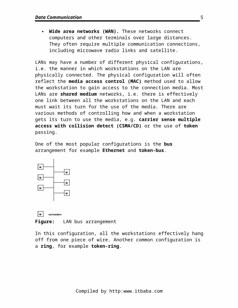
One of the most popular configurations is the bus arrangement for example Ethernet and token-bus.

Figure: LAN bus arrangement

In this configuration, all the workstations effectively hang off from one piece of wire. Another common configuration is a ring, for example token-ring.


4

Data Communication

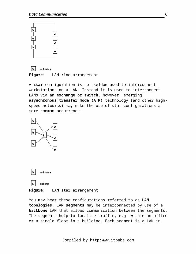
Figure: LAN ring arrangement

A star configuration is not seldom used to interconnect workstations on a LAN. Instead it is used to interconnect LANs via an exchange or switch, however, emerging asynchronous transfer mode (ATM) technology (and other high-speed networks) may make the use of star configurations a more common occurrence.

Figure: LAN star arrangement

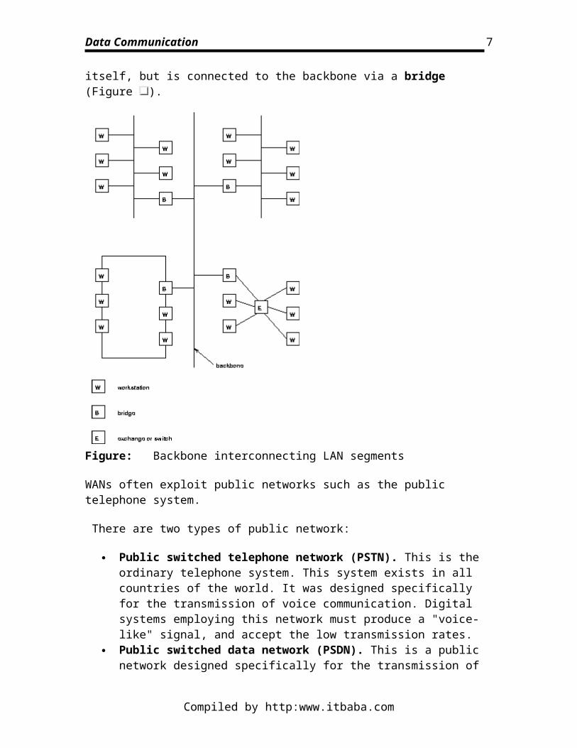
You may hear these configurations referred to as LAN topologies. LAN segments may be interconnected by use of a backbone LAN that allows communication between the segments. The segments help to localise traffic, e.g. within an office or a single floor in a building. Each segment is a LAN in itself, but is connected to the backbone via a bridge (Figure ).


5

http://www.cs.ucl.ac.uk/staff/S.Bhatti/D51-notes/node2.html#figbackbonelan

Data Communication

Figure: Backbone interconnecting LAN segments

WANs often exploit public networks such as the public telephone system.

There are two types of public network:

Public switched telephone network (PSTN). This is the ordinary telephone system. This system exists in all countries of the world. It was designed specifically for the transmission of voice communication. Digital systems employing this network must produce a "voice-like" signal, and accept the low transmission rates.

Public switched data network (PSDN). This is a public network designed specifically for the transmission of digital data. They arose from privately owned WANs that required higher performance than the PSTN. Many countries of the world are introducing PSDN services. They can support much higher transmission rates. An integrated services digital network (ISDN) is the term given to all-digital networks that can carry simultaneously voice and data communication, and offer additionally a variety of teletex services. ISDN services are being introduced all round the world and are indeed on offer in the UK.


6

Data Communication

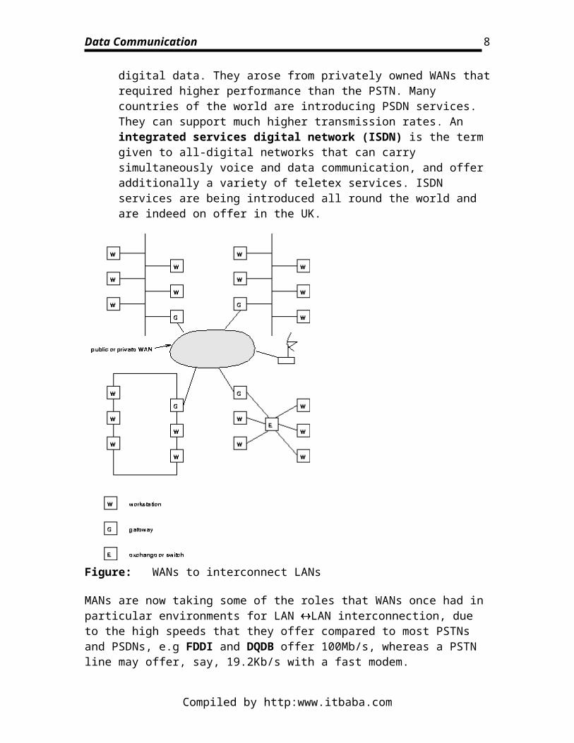
Figure: WANs to interconnect LANs

MANs are now taking some of the roles that WANs once had in particular environments for LAN LAN interconnection, due to the high speeds that they offer compared to most PSTNs and PSDNs, e.g FDDI and DQDB offer 100Mb/s, whereas a PSTN line may offer, say, 19.2Kb/s with a fast modem.

At the present time the world's communication systems are in a state of flux. Historically, digital computing equipment conformed to the requirements of the PSTN. Now, increasingly, analogue traffic such as voice and video is conforming to the requirements of the PSDN.

Public networks employ two types of switching. Switching describes the method by which the corresponders are connected. A circuit switched network (CSN) establishes a connection through the network that is then used exclusively by the two correspondents. (Of course, only in 19th century telephone exchanges is the switching actually current driven.) The PSTN is a circuit switched network. A packet switched network (PSN) divides the message into packets, which are addressed to the recipient. The packets are then forwarded through the network, together with many other packets. These are locally distributed on arrival. The Post Office is a packet switched network. More relevantly, LAN communication is exclusively via a PSN. The outstanding advantage of the PSN is


7

Data Communication

that the two correspondents can communicate at different rates, permitting much more efficient use of the communication channel.

The variety and description of telecommunications trafficTelecommunications traffic is characterized by great diversity. A non-exclusive list is the following:

Digital data is universally represented by strings of 1s or 0s. Each one or zero is referred to as a bit. Often, but not always, these bit strings are interpreted as numbers in a binary number system. Thus . The information content of a digital signal is equal to the number of bits required to represent it. Thus a signal that may vary between 0 and 7 has an information content of 3 bits. Written as an equation this relationship is:

where n is the number of levels a signal may take. It is important to appreciate that information is a measure of the number of different outcomes a value may take. Thus, the individual values 0 or 7 each have an information content of 1 bit; the range of integer values between 0 and 7 have an information content of 3 bits.

The information rate is a measure of the speed with which information is transferred. It is measured in b/s.

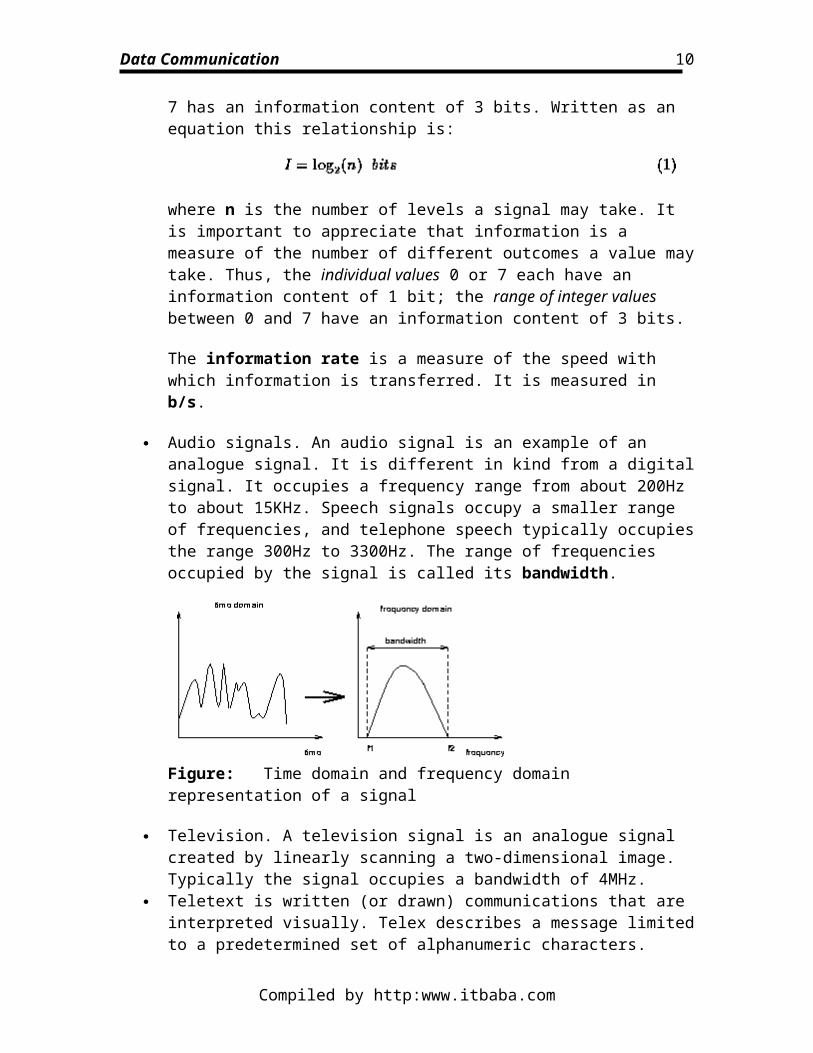
Audio signals. An audio signal is an example of an analogue signal. It is different in kind from a digital signal. It occupies a frequency range from about 200Hz to about 15KHz. Speech signals occupy a smaller range of frequencies, and telephone speech typically occupies the range 300Hz to 3300Hz. The range of frequencies occupied by the signal is called its bandwidth.

Figure: Time domain and frequency domain representation of a signal


8

Data Communication

Television. A television signal is an analogue signal created by linearly scanning a two-dimensional image. Typically the signal occupies a bandwidth of 4MHz.

Teletext is written (or drawn) communications that are interpreted visually. Telex describes a message limited to a predetermined set of alphanumeric characters. Facsimile describes the transmission of documents that have been converted into a discrete two-tone image.

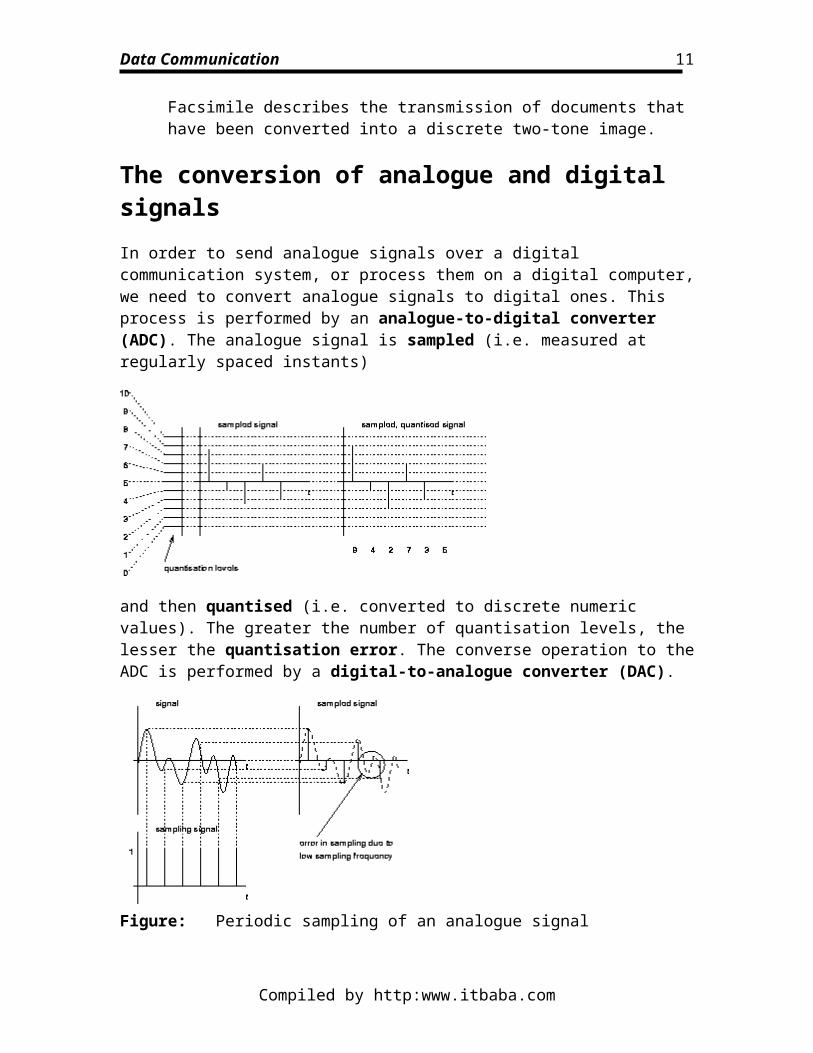
The conversion of analogue and digital signalsIn order to send analogue signals over a digital communication system, or process them on a digital computer, we need to convert analogue signals to digital ones. This process is performed by an analogue-to-digital converter (ADC). The analogue signal is sampled (i.e. measured at regularly spaced instants)

and then quantised (i.e. converted to discrete numeric values). The greater the number of quantisation levels, the lesser the quantisation error. The converse operation to the ADC is performed by a digital-to-analogue converter (DAC).

Figure: Periodic sampling of an analogue signal


9

Data Communication

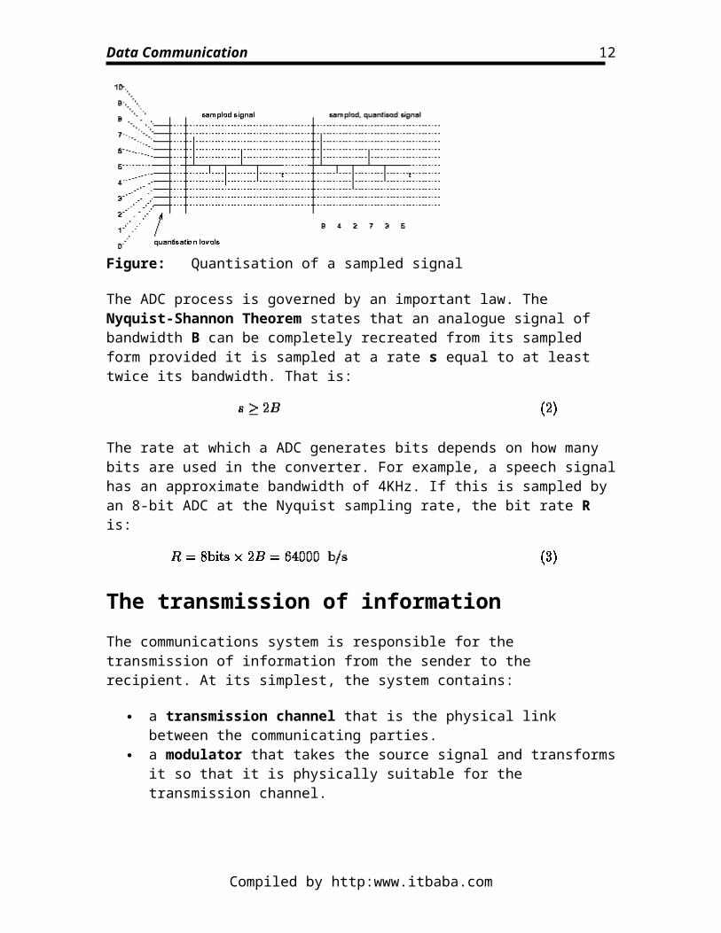
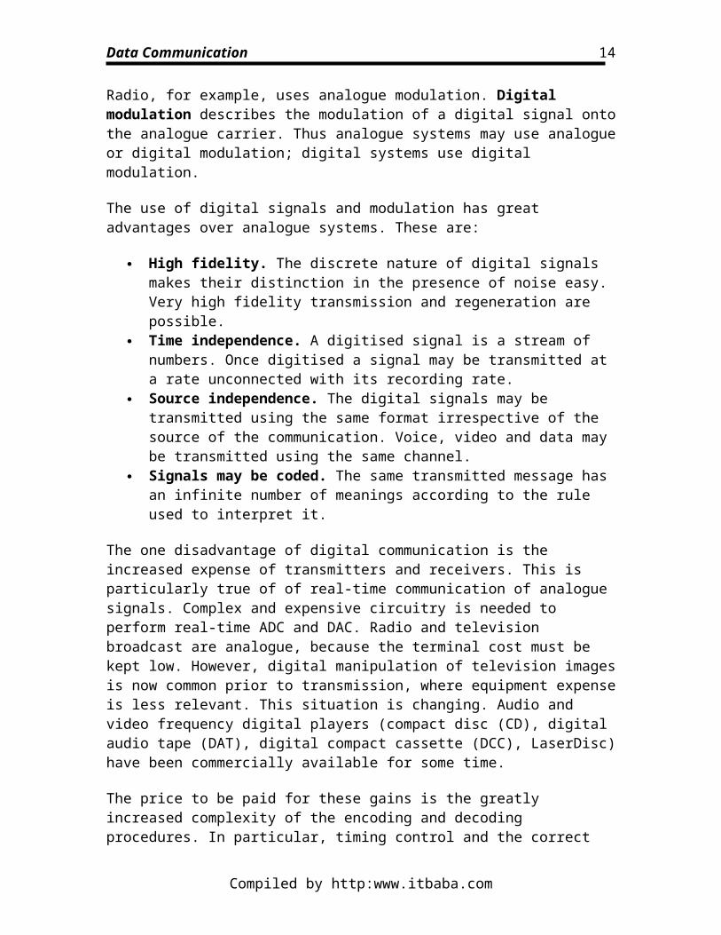
Figure: Quantisation of a sampled signal

The ADC process is governed by an important law. The Nyquist-Shannon Theorem states that an analogue signal of bandwidth B can be completely recreated from its sampled form provided it is sampled at a rate s equal to at least twice its bandwidth. That is:

The rate at which a ADC generates bits depends on how many bits are used in the converter. For example, a speech signal has an approximate bandwidth of 4KHz. If this is sampled by an 8-bit ADC at the Nyquist sampling rate, the bit rate R is:

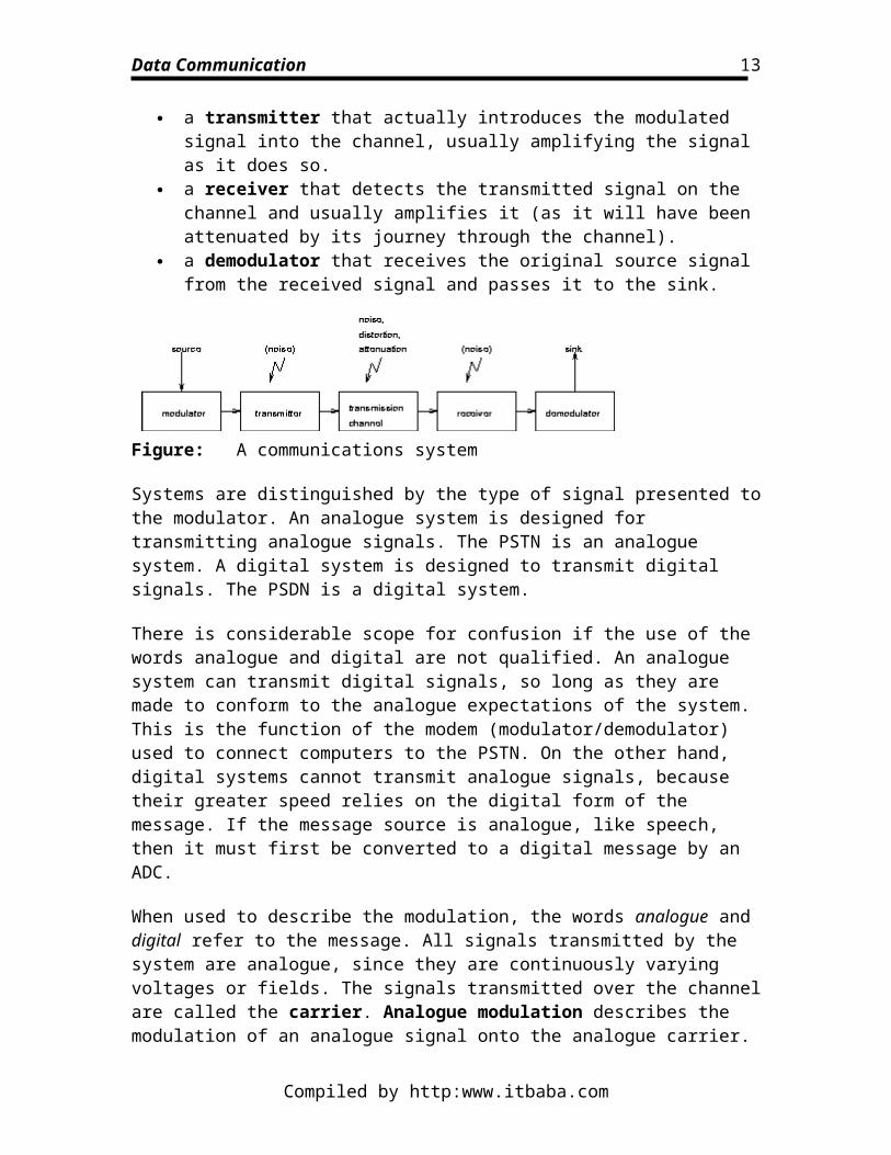
The transmission of informationThe communications system is responsible for the transmission of information from the sender to the recipient. At its simplest, the system contains:

a transmission channel that is the physical link between the communicating parties.

a modulator that takes the source signal and transforms it so that it is physically suitable for the transmission channel.

a transmitter that actually introduces the modulated signal into the channel, usually amplifying the signal as it does so.

a receiver that detects the transmitted signal on the channel and usually amplifies it (as it will have been attenuated by its journey through the channel).

a demodulator that receives the original source signal from the received signal and passes it to the sink.


10

Data Communication

Figure: A communications system

Systems are distinguished by the type of signal presented to the modulator. An analogue system is designed for transmitting analogue signals. The PSTN is an analogue system. A digital system is designed to transmit digital signals. The PSDN is a digital system.

There is considerable scope for confusion if the use of the words analogue and digital are not qualified. An analogue system can transmit digital signals, so long as they are made to conform to the analogue expectations of the system. This is the function of the modem (modulator/demodulator) used to connect computers to the PSTN. On the other hand, digital systems cannot transmit analogue signals, because their greater speed relies on the digital form of the message. If the message source is analogue, like speech, then it must first be converted to a digital message by an ADC.

When used to describe the modulation, the words analogue and digital refer to the message. All signals transmitted by the system are analogue, since they are continuously varying voltages or fields. The signals transmitted over the channel are called the carrier. Analogue modulation describes the modulation of an analogue signal onto the analogue carrier. Radio, for example, uses analogue modulation. Digital modulation describes the modulation of a digital signal onto the analogue carrier. Thus analogue systems may use analogue or digital modulation; digital systems use digital modulation.

The use of digital signals and modulation has great advantages over analogue systems. These are:

High fidelity. The discrete nature of digital signals makes their distinction in the presence of noise easy. Very high fidelity transmission and regeneration are possible.

Time independence. A digitised signal is a stream of numbers. Once digitised a signal may be transmitted at a rate unconnected with its recording rate.

Source independence. The digital signals may be transmitted using the same format irrespective of the source of the communication. Voice, video and data may be transmitted using the same channel.

Signals may be coded. The same transmitted message has an infinite number of meanings according to the rule used to interpret it.

The one disadvantage of digital communication is the increased expense of transmitters and receivers. This is particularly true of of real-time communication of analogue signals. Complex and expensive circuitry is needed to perform real-time ADC and DAC. Radio and television broadcast are analogue, because the terminal cost must be kept low.


11

Data Communication

However, digital manipulation of television images is now common prior to transmission, where equipment expense is less relevant. This situation is changing. Audio and video frequency digital players (compact disc (CD), digital audio tape (DAT), digital compact cassette (DCC), LaserDisc) have been commercially available for some time.

The price to be paid for these gains is the greatly increased complexity of the encoding and decoding procedures. In particular, timing control and the correct identification of the digital structure are crucial. These problems do not exist with analogue communication.

The relationship between information, bandwidth and noiseThe most important question associated with a communication channel is the maximum rate at which it can transfer information. Information can only be transferred by a signal if the signal is permitted to change. Analogue signals passing through physical channels may not change arbitrarily fast. The rate at which a signal may change is determined by the bandwidth. In fact it is governed by the same Nyquist-Shannon law as governs sampling; a signal of bandwidth B may change at a maximum rate of 2B. If each change is used to signify a bit, the maximum information rate is 2B.

The Nyquist-Shannon theorem makes no observation concerning the magnitude of the change. If changes of differing magnitude are each associated with a separate bit, the information rate may be increased. Thus, if each time the signal changes it can take one of n levels, the information rate is increased to:

This formula states that as n tends to infinity, so does the information rate.

Is there a limit on the number of levels? The limit is set by the presence of noise. If we continue to subdivide the magnitude of the changes into ever decreasing intervals, we reach a point where we cannot distinguish the individual levels because of the presence of noise. Noise therefore places a limit on the maximum rate at which we can transfer information. Obviously, what really matters is the signal-to-noise ratio (SNR). This is defined by the ratio of signal power S to noise power N, and is often expressed in deciBels;

Also note that it is common to see following expressions for power in many texts:


12

Data Communication

i.e. equation expresses power as a ratio to 1 Watt and expresses power as a ratio to 1 milliWatt. These are expressions of power and should not be confused with SNR.

There is a theoretical maximum to the rate at which information passes error free over the channel. This maximum is called the channel capacity C. The famous Hartley-Shannon Law states that the channel capacity C is given by:

Note that S/N is linear in this expression. For example, a 10KHz channel operating in a SNR of 15dB has a theoretical maximum information rate of

b/s.

The theorem makes no statement as to how the channel capacity is achieved. In fact, channels only approach this limit. The task of providing high channel efficiency is the goal of coding techniques. The failure to meet perfect performance is measured by the bit-error-rate (BER). Typically BERs are of the order .

The description and types of communication channelsThe communication channel is a crucial part of the communication network. It is an analogue part of the system, and is described in terms of the analogue -- quantities bandwidth, absorption etc. It limits the bandwidth and noise power, which we have already identified as factors determining the maximum information rate of the channel. Additionally, the channel can introduce various kinds of distortion into the signal, and also has a delay associated with it.

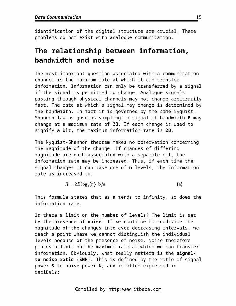
When a signal is introduced into a channel of bandwidth B, the signal emerging from the end of a channel has its bandwidth reduced to the bandwidth B of the channel. Signals lying outside the bandwidth of the channel are removed. The channel places a maximum value of the bandwidth of the system, irrespective of the signal bandwidth. According to the type and length of the channel, the bandwidth will be determined (Figure ).

Figure: The effects of limited bandwidth

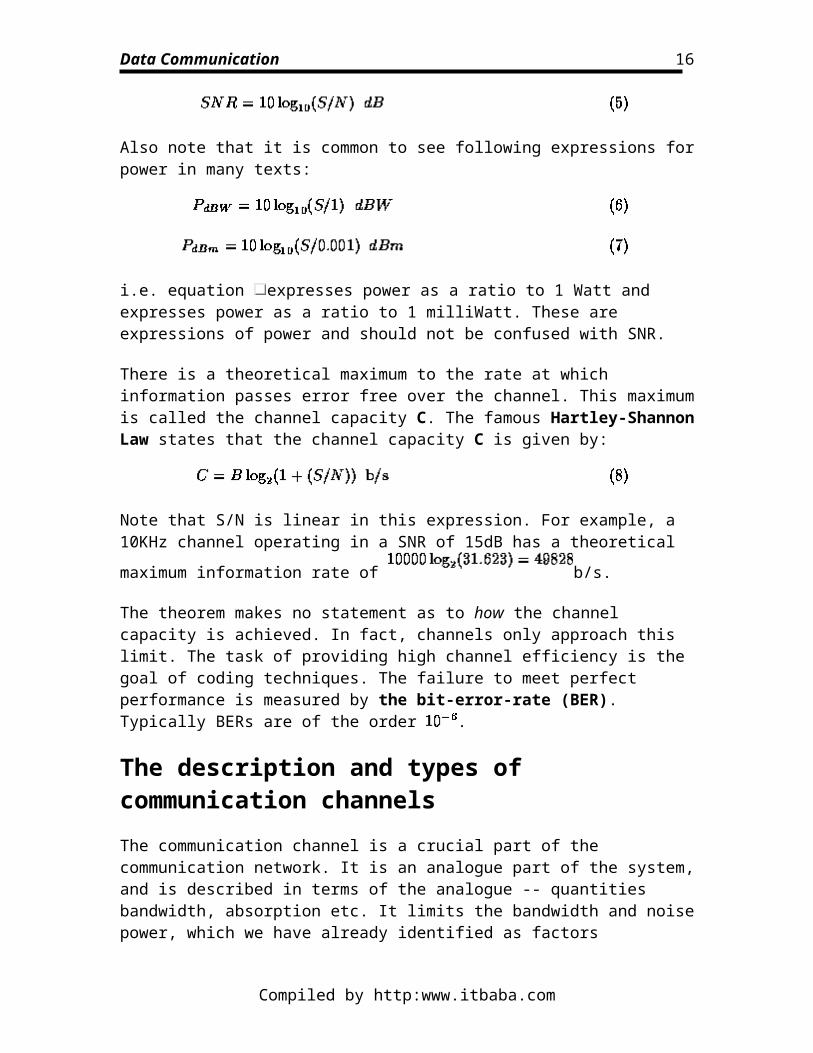
Absorption is the term used to describe the loss of signal power as the signal moves through the channel (Figure ). The longer the channel, the higher the absorption. It is

usually specified in . Absorption is usually frequency dependent. It reduces the available bandwidth. Equalisers are frequency dependent amplifiers that restore the spectral balance of the signal.


13

http://www.cs.ucl.ac.uk/staff/S.Bhatti/D51-notes/node6.html#equPdBW

http://www.cs.ucl.ac.uk/staff/S.Bhatti/D51-notes/node7.html#figlimitedbandwidth

http://www.cs.ucl.ac.uk/staff/S.Bhatti/D51-notes/node7.html#figabsorption

Data Communication

Figure: The effects of channel absorption

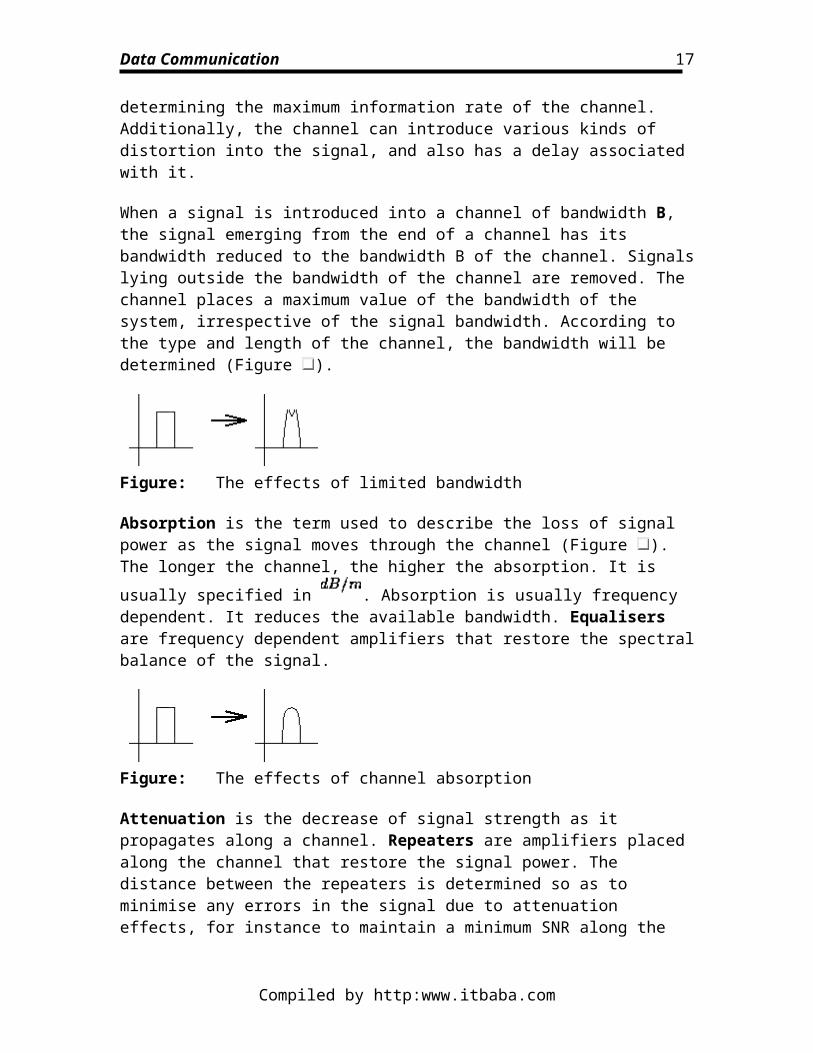
Attenuation is the decrease of signal strength as it propagates along a channel. Repeaters are amplifiers placed along the channel that restore the signal power. The distance between the repeaters is determined so as to minimise any errors in the signal due to attenuation effects, for instance to maintain a minimum SNR along the channel (Figure ). Some attenuation affects are due to absorption. The amount of attentuation is

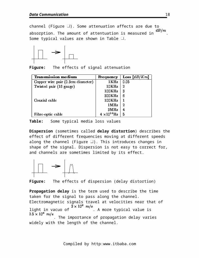
measured in . Some typical values are shown in Table .

Figure: The effects of signal attenuation

Table: Some typical media loss values

Dispersion (sometimes called delay distortion) describes the effect of different frequencies moving at different speeds along the channel (Figure ). This introduces changes in shape of the signal. Dispersion is not easy to correct for, and channels are sometimes limited by its effect.

Figure: The effects of dispersion (delay distortion)

Propagation delay is the term used to describe the time taken for the signal to pass along the channel. Electromagnetic signals travel at velocities near that of light in vacuo of


14

http://www.cs.ucl.ac.uk/staff/S.Bhatti/D51-notes/node7.html#figattenuation

http://www.cs.ucl.ac.uk/staff/S.Bhatti/D51-notes/node7.html#tblattenuation

http://www.cs.ucl.ac.uk/staff/S.Bhatti/D51-notes/node7.html#figdispersion

Data Communication

. A more typical value is . The importance of propagation delay varies widely with the length of the channel.

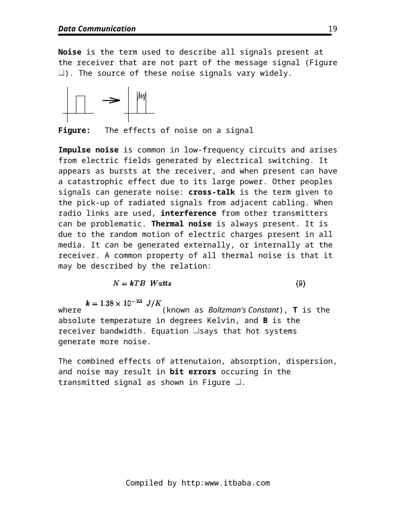
Noise is the term used to describe all signals present at the receiver that are not part of the message signal (Figure ). The source of these noise signals vary widely.

Figure: The effects of noise on a signal

Impulse noise is common in low-frequency circuits and arises from electric fields generated by electrical switching. It appears as bursts at the receiver, and when present can have a catastrophic effect due to its large power. Other peoples signals can generate noise: cross-talk is the term given to the pick-up of radiated signals from adjacent cabling. When radio links are used, interference from other transmitters can be problematic. Thermal noise is always present. It is due to the random motion of electric charges present in all media. It can be generated externally, or internally at the receiver. A common property of all thermal noise is that it may be described by the relation:

where (known as Boltzman's Constant), T is the absolute temperature in degrees Kelvin, and B is the receiver bandwidth. Equation says that hot systems generate more noise.

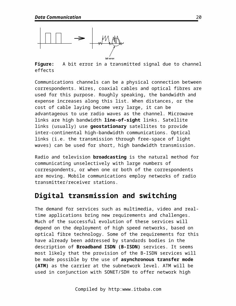
The combined effects of attenutaion, absorption, dispersion, and noise may result in bit errors occuring in the transmitted signal as shown in Figure .

Figure: A bit error in a transmitted signal due to channel effects

Communications channels can be a physical connection between correspondents. Wires, coaxial cables and optical fibres are used for this purpose. Roughly speaking, the bandwidth and expense increases along this list. When distances, or the cost of cable laying become very large, it can be advantageous to use radio waves as the channel. Microwave links are high bandwidth line-of-sight links. Satellite links (usually) use geostationary satellites to provide inter-continental high-bandwidth communications.


15

http://www.cs.ucl.ac.uk/staff/S.Bhatti/D51-notes/node7.html#fignoise

http://www.cs.ucl.ac.uk/staff/S.Bhatti/D51-notes/node7.html#equThermalNoise

http://www.cs.ucl.ac.uk/staff/S.Bhatti/D51-notes/node7.html#figsignaltx

Data Communication

Optical links (i.e. the transmission through free-space of light waves) can be used for short, high bandwidth transmission.

Radio and television broadcasting is the natural method for communicating unselectively with large numbers of correspondents, or when one or both of the correspondents are moving. Mobile communications employ networks of radio transmitter/receiver stations.

Digital transmission and switchingThe demand for services such as multimedia, video and real-time applications bring new requirements and challenges. Much of the successful evolution of these services will depend on the deployment of high speed networks, based on optical fibre technology. Some of the requirements for this have already been addressed by standards bodies in the description of Broadband ISDN (B-ISDN) services. It seems most likely that the provision of the B-ISDN services will be made possible by the use of asynchronous transfer mode (ATM) as the carrier at the subnetwork level. ATM will be used in conjunction with SONET/SDH to offer network high speed network services, with rates of 155Mb/s to 622Mb/s (and higher) being planned. Synchronous Optical Network (SONET) and Synchronous Digital Hierarchy (SDH) are two similar architectures proposed for using ATM based networks, the latter (a European standard) being based heavily on the former (a US standard).

With the real-time applications that need to run over large, diverse networks, issues arise concerning the Quality of Service (QoS) guarantees required from the network in order to maintain the required network resources for the needs of a particular application. Most of the current activity in this increasingly popular area of research focus around providing models for QoS in terms of various parameters such as speed, delay, jitter and various error rates.

To fully exploit the huge bandwidth offered by optical fibre technology we require electronic equipment that will be able to operate at speeds of at least the rate of optical transmission. Currently, our use of the optical bandwidths is limited by the electronic technology that is used for transmitting and receiving the signals, as the electronic components used approach the operational limits of their fabrication techniques, e.g. CMOS. The electronic components not only restrict the way in which the information is actually transmitted into the fibre (the type of signal modulation used), but also the speed at which information is switched between the links that make up the network.

Network switches are crucial elements in the provision of high speed networks. Switches link the physical paths which the data takes through the network. Although it may be possible to build on known switching techniques and improve their throughput, with the increasing speed of transmission of the data, the switches must also become faster if they are not to become performance bottlenecks in the evolution of high speed networks.


16

Data Communication

StandardsInternational bodies concerned with the interconnection of telecommunications equipment have for decades provided standards for the connection of terminals to these lines. These systems were initially analogue, and the associated standards were primarily concerned with defining the hardware and electrical interfaces. V-series standards relate to the connection of terminals to PSTNs, D-series to PSDN's and I-series to ISDNs. The X-series recommendations relate to network services and protocols that are independent of the underlying subnetwork technology. This in marked contrast to computer manufacturers, who in the past have tended to introduce internal standards that make different manufactures equipment incompatible. Such systems are described as closed systems, in contrast to the open systems of the telephone networks.

The recognition that compatibility was potentially advantageous led to the formation of the International Organisation for Standardisation (ISO). This body has generated a range of standards concerning the connection of computer equipment, the connection of LANs, the connection of equipment and LANs to PSDNs, and more recently the connection to the higher level functions of the ISDNs. ISO works in close collaboration with the ITU-TSS (International Telecommunications Union-Telecommunication Standardization Sector), which was formerly the CCITT (International Consultative Committee for Telephony and Telegraphy). These groups receive contributions and suggestions from various national bodies, such as BSI (British Standards Institute) and ANSI (American National Standards Institute), IEEE (Institute of Electrical and Electronic Engineers), as well as from commercial companies with interest in the areas to be standardised. ANSI and IEEE also produce their own documents which are often adopted as ISO or CCITT standards.

While these international standards bodies are important, they are not the only people involved with the promotion of the the use of data communications technologies. Indeed, the largest network in the world, the Internet uses standards that were developed within its own community, consisting originally of many universities and research establishments. The Internet continues to encourage the publishing of its Request For Comments (RFC) documents that are available freely to anyone with Internet access.

Many other groups are concerned with the use of standards or producing profiles for architectures based on existing standards for instance the Network Management Forum (NMF) and the Open Software Foundation (OSF). These two organisations are particularly interested in promoting agreements that will encourage use and interoperability of 'open' standards.

Time, frequency and bandwidthPreviously, the ideas of the frequency content and bandwidth of an analogue signal were introduced. In this section, we wish to examine these ideas more closely.


17

Data Communication

Most signals carried by communication channels are modulated forms of sine waves. A sine wave is described mathematically by the expression:

The quantities A, , and are termed the amplitude, frequency and phase of the sine wave, respectively. We can describe this signal in two ways. One way is to describe its evolution in time (time domain model), and equation is a mathematical representation of this evolution. The second way is to describe its frequency content (frequency domain model). The sine wave has a single frequency, .

This representation is quite general. In fact we have the following theorem due to Fourier:

Any signal of time may be represented as the sum of a set of sine waves of different frequencies and phases.

Mathematically:

The frequency description of this signal would describe the amplitudes as a function of the frequency . The description of a signal in terms of its constituent frequencies is called its frequency spectrum.

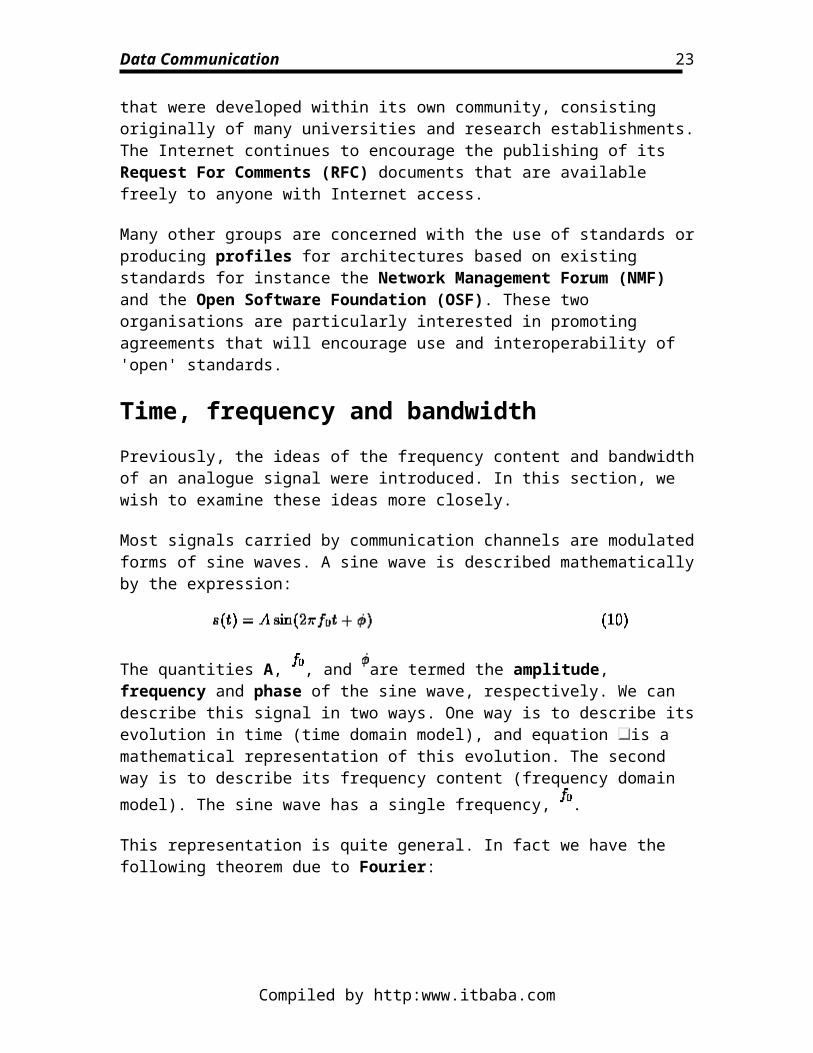
As an example, consider the square wave (Figure ):

Figure: A square wave

This has the Fourier series:


18

http://www.cs.ucl.ac.uk/staff/S.Bhatti/D51-notes/node11.html#equsin

http://www.cs.ucl.ac.uk/staff/S.Bhatti/D51-notes/node11.html#figsquarewave

Data Communication

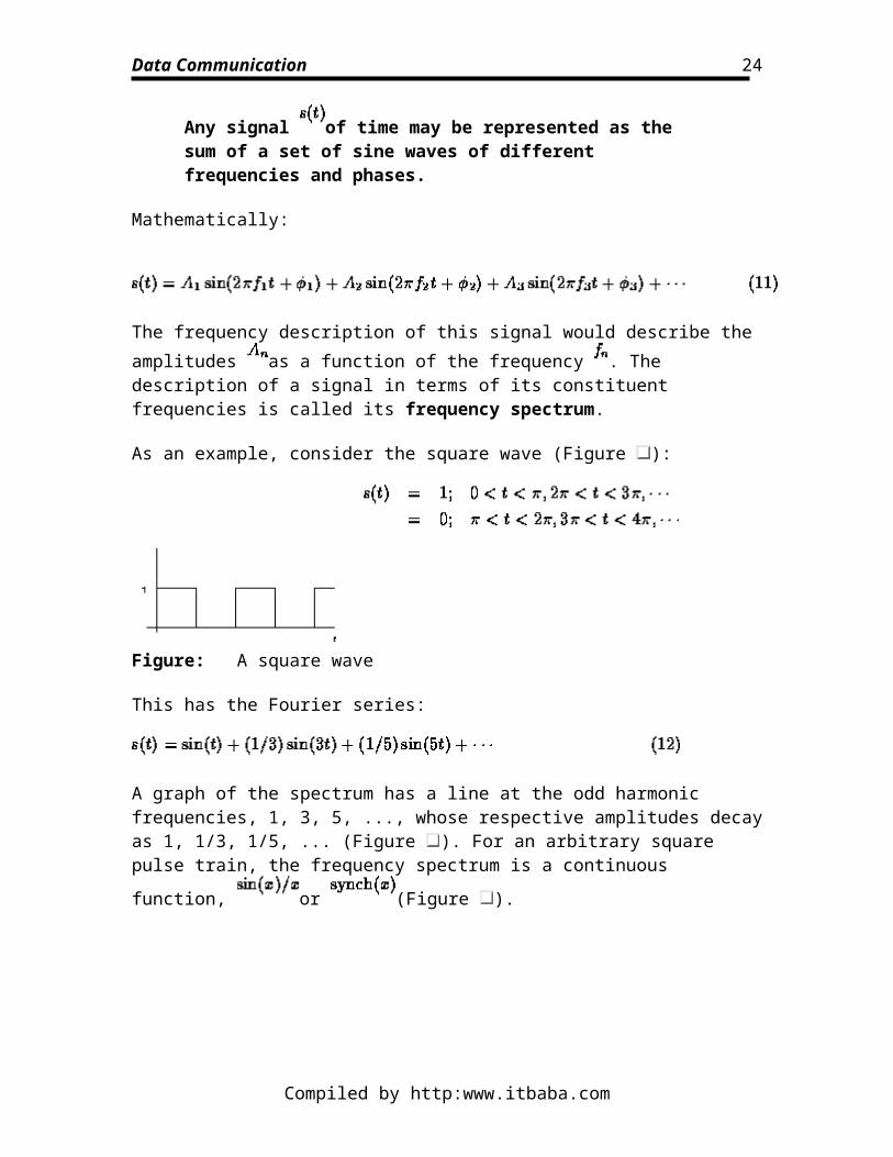
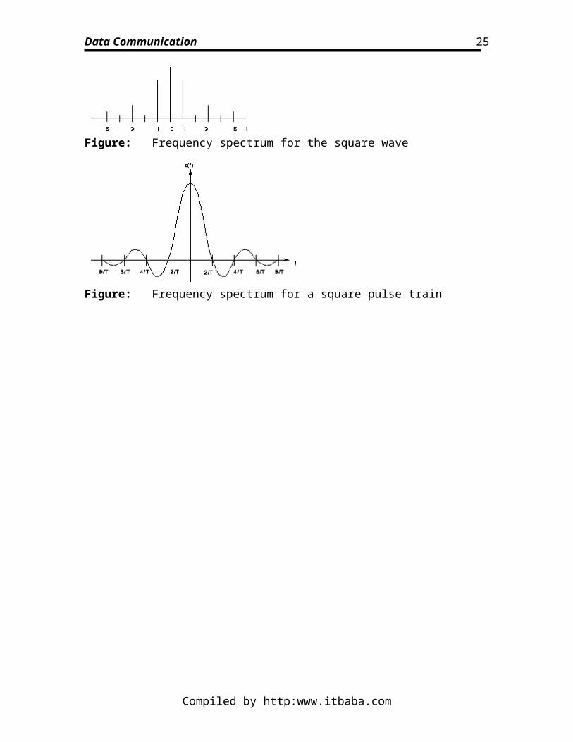
A graph of the spectrum has a line at the odd harmonic frequencies, 1, 3, 5, ..., whose respective amplitudes decay as 1, 1/3, 1/5, ... (Figure ). For an arbitrary square pulse

train, the frequency spectrum is a continuous function, or (Figure ).

Figure: Frequency spectrum for the square wave

Figure: Frequency spectrum for a square pulse train


19

http://www.cs.ucl.ac.uk/staff/S.Bhatti/D51-notes/node11.html#figsquarespectrum

http://www.cs.ucl.ac.uk/staff/S.Bhatti/D51-notes/node11.html#figsynch

Data Communication

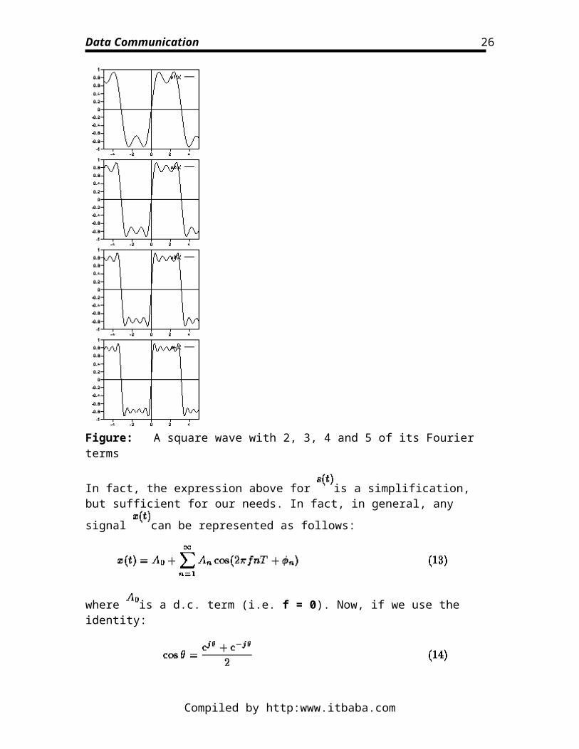
Figure: A square wave with 2, 3, 4 and 5 of its Fourier terms

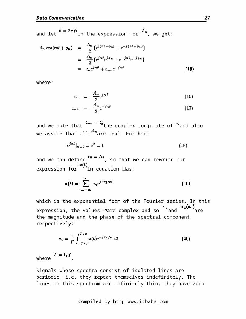
In fact, the expression above for is a simplification, but sufficient for our needs. In

fact, in general, any signal can be represented as follows:

where is a d.c. term (i.e. f = 0). Now, if we use the identity:

and let in the expression for , we get:


20

Data Communication

where:

and we note that the complex conjugate of and also we assume that all are real. Further:

and we can define , so that we can rewrite our expression for in equation as:

which is the exponential form of the Fourier series. In this expression, the values are

complex and so and are the magnitude and the phase of the spectral component respectively:

where .

Signals whose spectra consist of isolated lines are periodic, i.e. they repeat themselves indefinitely. The lines in this spectrum are infinitely thin; they have zero bandwidth. The Hartley-Shannon law (equation ) tells us that the maximum information rate of a zero bandwidth channel is zero. Thus, zero bandwidth signals carry no information.

To permit the signal to carry information we must introduce the capacity for aperiodic change. The consequence of an aperiodic change is to introduce a spread of frequencies into the signal. Detailed theoretical consideration leads us to the Nyquist-Shannon law


21

http://www.cs.ucl.ac.uk/staff/S.Bhatti/D51-notes/node11.html#equFouriercos

http://www.cs.ucl.ac.uk/staff/S.Bhatti/D51-notes/node6.html#equHartleyShannon

Data Communication

that a signal of bandwidth B may change in an aperiodic fashion at a maximum rate of 2B (equation ).

If the square-wave signal discussed in the previous example is replaced with an aperiodic sequence of 1s and 0s, the spectrum changes substantially. The discrete harmonic components are replaced by a continuous range of frequencies whose shape is a synch function. There a number of features to note:

The bandwidth of the signal is only approximately finite. Most of the energy is contained in a limited region called the main-lobe. However, some energy is found at all frequencies.

If there are two changes in the period T, the width of the main-lobe is . The

Nyquist-Shannon law (equation ) states that if a signal has bandwidth , then

the maximum number of changes that may take place is per second, or 8 changes in the period T. If each change is taken to represent 1 bit, it is apparent that this signal does not carry as much information as the bandwidth permits.

The spectrum has positive and negative frequencies. These are symmetric about the origin. This may seem non-intuitive but can be seen from equation .

The bandwidth of a communication channel is limited by the physical construction of the channel. The Nyquist-Shannon law places a limit on the maximum number of aperiodic changes per unit time the signal may perform. It is the task of the modulator to make best use of the available bandwidth. However, the modulator is itself constrained by its physical design and construction, and it may or may not approach the Nyquist limit in its operation.

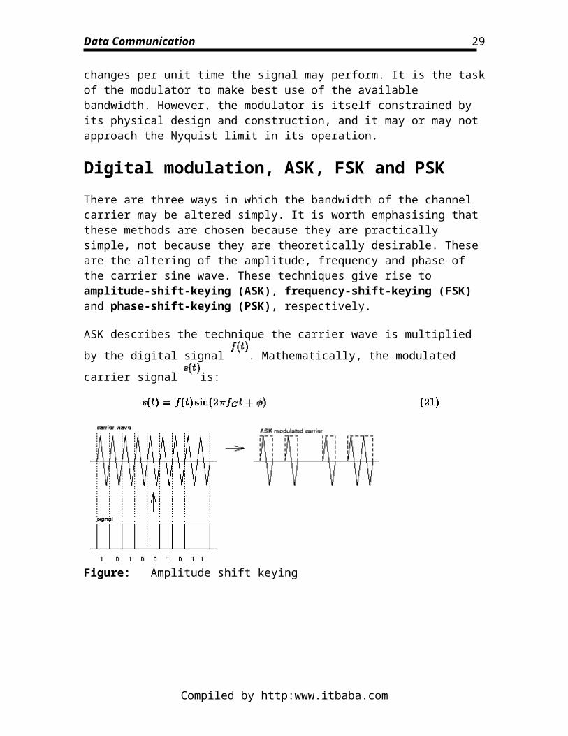
Digital modulation, ASK, FSK and PSKThere are three ways in which the bandwidth of the channel carrier may be altered simply. It is worth emphasising that these methods are chosen because they are practically simple, not because they are theoretically desirable. These are the altering of the amplitude, frequency and phase of the carrier sine wave. These techniques give rise to amplitude-shift-keying (ASK), frequency-shift-keying (FSK) and phase-shift-keying (PSK), respectively.

ASK describes the technique the carrier wave is multiplied by the digital signal .

Mathematically, the modulated carrier signal is:


22

http://www.cs.ucl.ac.uk/staff/S.Bhatti/D51-notes/node4.html#equNyquistShannon

http://www.cs.ucl.ac.uk/staff/S.Bhatti/D51-notes/node4.html#equNyquistShannon

http://www.cs.ucl.ac.uk/staff/S.Bhatti/D51-notes/node11.html#equFourierexp

Data Communication

Figure: Amplitude shift keying

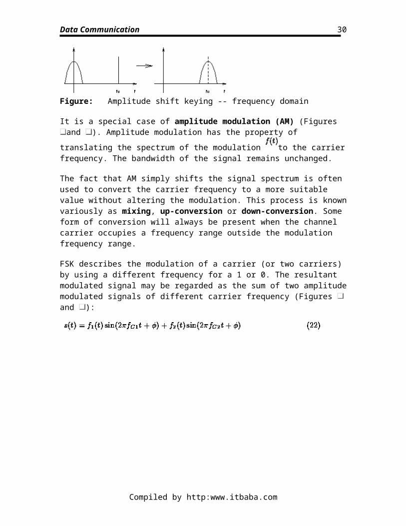
Figure: Amplitude shift keying -- frequency domain

It is a special case of amplitude modulation (AM) (Figures and ). Amplitude

modulation has the property of translating the spectrum of the modulation to the carrier frequency. The bandwidth of the signal remains unchanged.

The fact that AM simply shifts the signal spectrum is often used to convert the carrier frequency to a more suitable value without altering the modulation. This process is known variously as mixing, up-conversion or down-conversion. Some form of conversion will always be present when the channel carrier occupies a frequency range outside the modulation frequency range.

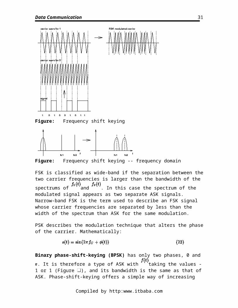
FSK describes the modulation of a carrier (or two carriers) by using a different frequency for a 1 or 0. The resultant modulated signal may be regarded as the sum of two amplitude modulated signals of different carrier frequency (Figures and ):


23

http://www.cs.ucl.ac.uk/staff/S.Bhatti/D51-notes/node12.html#figask

http://www.cs.ucl.ac.uk/staff/S.Bhatti/D51-notes/node12.html#figaskf

http://www.cs.ucl.ac.uk/staff/S.Bhatti/D51-notes/node12.html#figfsk

http://www.cs.ucl.ac.uk/staff/S.Bhatti/D51-notes/node12.html#figfskf

Data Communication

Figure: Frequency shift keying

Figure: Frequency shift keying -- frequency domain

FSK is classified as wide-band if the separation between the two carrier frequencies is

larger than the bandwidth of the spectrums of and . In this case the spectrum of the modulated signal appears as two separate ASK signals. Narrow-band FSK is the term used to describe an FSK signal whose carrier frequencies are separated by less than the width of the spectrum than ASK for the same modulation.

PSK describes the modulation technique that alters the phase of the carrier. Mathematically:

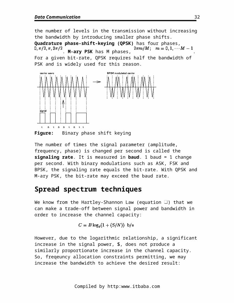
Binary phase-shift-keying (BPSK) has only two phases, 0 and . It is therefore a type of

ASK with taking the values -1 or 1 (Figure ), and its bandwidth is the same as that of ASK. Phase-shift-keying offers a simple way of increasing the number of levels in the transmission without increasing the bandwidth by introducing smaller phase shifts.

Quadrature phase-shift-keying (QPSK) has four phases, . M-ary PSK

has M phases, . For a given bit-rate, QPSK requires half the bandwidth of PSK and is widely used for this reason.


24

http://www.cs.ucl.ac.uk/staff/S.Bhatti/D51-notes/node12.html#figbpsk

Data Communication

Figure: Binary phase shift keying

The number of times the signal parameter (amplitude, frequency, phase) is changed per second is called the signaling rate. It is measured in baud. 1 baud = 1 change per second. With binary modulations such as ASK, FSK and BPSK, the signaling rate equals the bit-rate. With QPSK and M-ary PSK, the bit-rate may exceed the baud rate.

Spread spectrum techniquesWe know from the Hartley-Shannon Law (equation ) that we can make a trade-off between signal power and bandwidth in order to increase the channel capacity:

However, due to the logarithmic relationship, a significant increase in the signal power, S, does not produce a similarly proportionate increase in the channel capacity. So, freqeuncy allocation constraints permitting, we may increase the bandwidth to achieve the desired result:

with the last step in the above derivation is made by using the logarithmic expansion:

with . Since is typically of the order of 0.1 in spread spectrum techniques, we consider all terms in the expansion except the first as negligible. So, for instance, for a


25


Data Communication

32Kb/s channel with a SNR of 0.001 (-30dB), B 22MHz. The two main criteria for using spread spectrum are:

The transmitted bandwidth is much greater that the minimum bandwidth that the signal requires (as given by the Hartley-Shannon Law).

Some function other than the information being sent determines the radio frequency bandwidth.

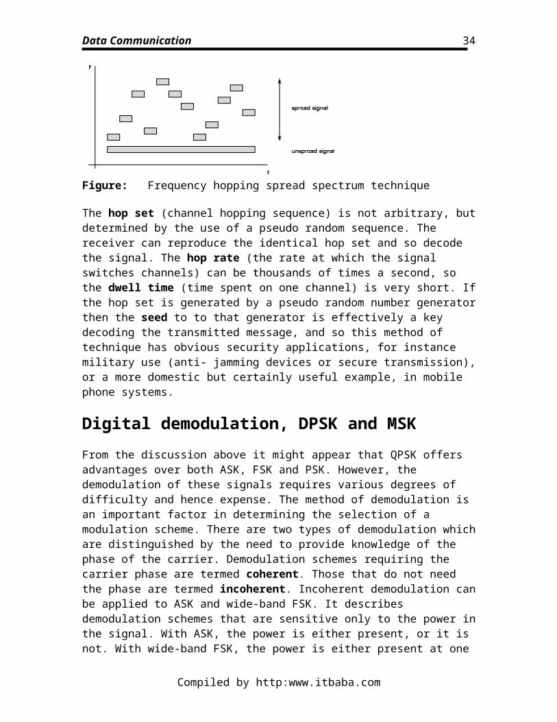
The first of these criteria has been demonstrated. The second criteria is determined by the type of modulation technique used. Cleary, incoherent modulation techniques by themselves will not be useful as the noise power is higher than the signal power! we shall not delve deeply into mechanisms, but shall look at one particular technique that is used called frequency hopping. In frequency hoping, the large bandwidth is effectively split into frequency channels. The signal is then spread across the channels as shown in Figure

.

Figure: Frequency hopping spread spectrum technique

The hop set (channel hopping sequence) is not arbitrary, but determined by the use of a pseudo random sequence. The receiver can reproduce the identical hop set and so decode the signal. The hop rate (the rate at which the signal switches channels) can be thousands of times a second, so the dwell time (time spent on one channel) is very short. If the hop set is generated by a pseudo random number generator then the seed to to that generator is effectively a key decoding the transmitted message, and so this method of technique has obvious security applications, for instance military use (anti- jamming devices or secure transmission), or a more domestic but certainly useful example, in mobile phone systems.

Digital demodulation, DPSK and MSKFrom the discussion above it might appear that QPSK offers advantages over both ASK, FSK and PSK. However, the demodulation of these signals requires various degrees of difficulty and hence expense. The method of demodulation is an important factor in determining the selection of a modulation scheme. There are two types of demodulation which are distinguished by the need to provide knowledge of the phase of the carrier. Demodulation schemes requiring the carrier phase are termed coherent. Those that do not need the phase are termed incoherent. Incoherent demodulation can be applied to


26

http://www.cs.ucl.ac.uk/staff/S.Bhatti/D51-notes/node13.html#figspreadspectrum

Data Communication

ASK and wide-band FSK. It describes demodulation schemes that are sensitive only to the power in the signal. With ASK, the power is either present, or it is not. With wide-band FSK, the power is either present at one frequency, or the other. Incoherent modulation is inexpensive but has poorer performance. Coherent demodulation requires more complex circuitry, but has better performance.

In ASK incoherent demodulation, the signal is passed to an envelope detector. This a device that outputs the "outline" of the signal. A decision is made as to whether the signal is present or not. Envelope detection is the simplest and cheapest method of demodulation. In optical communications, phase modulation is technically very difficult, and ASK is the only option. In the electrical and microwave context, however, it is considered crude. In addition, systems where the signal amplitude may vary unpredictably, such as microwave links, are not suitable for ASK modulation.

Incoherent demodulation can also be used for wide-band FSK. Here the signals are passed to two circuits, each sensitive to one of the two carrier frequencies. Circuits whose output depends on the frequency of the input are called discriminators or filters. The outputs of the two discriminators are interrogated to determine the signal. Incoherent FSK demodulation is simple and cheap, but very wasteful of bandwidth. The signal must

be wide-band FSK to ensure the two signals and are distinguished. It is used in circumstances where bandwidth is not the primary constraint.

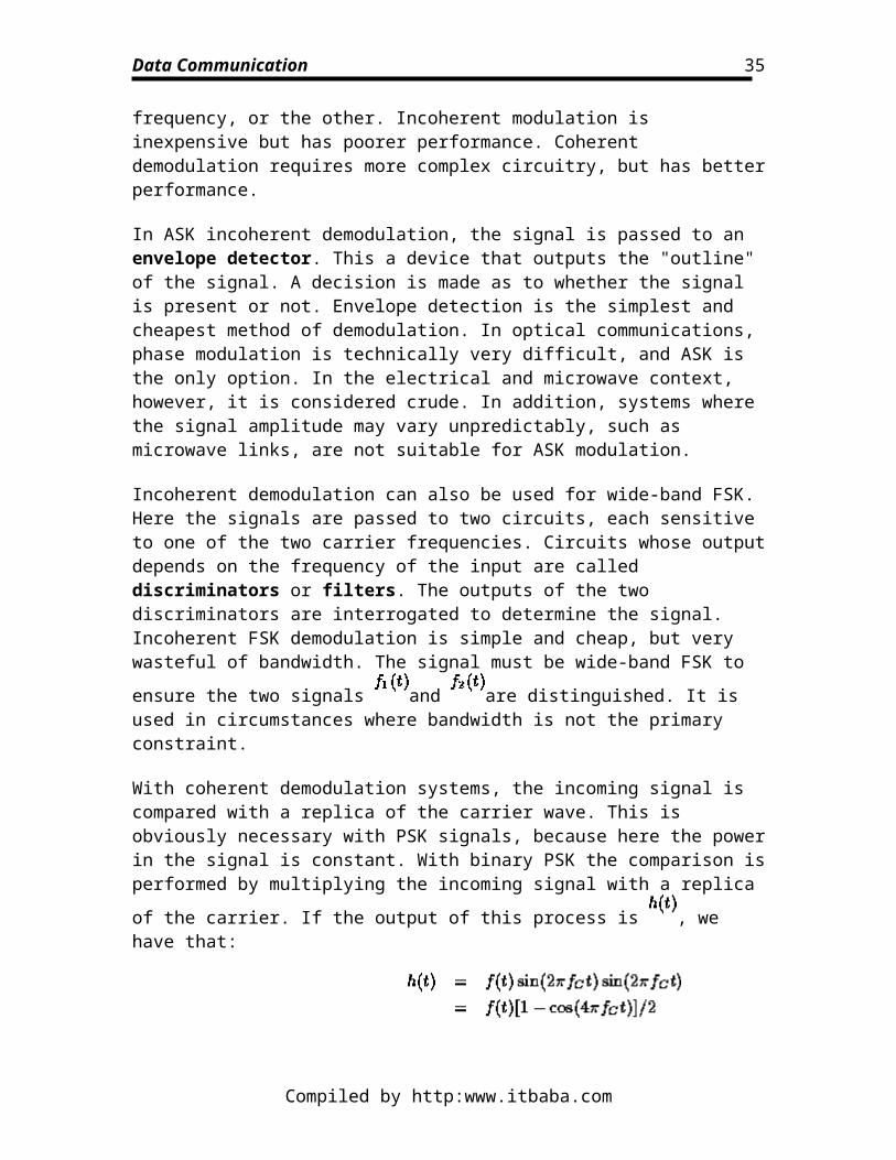
With coherent demodulation systems, the incoming signal is compared with a replica of the carrier wave. This is obviously necessary with PSK signals, because here the power in the signal is constant. With binary PSK the comparison is performed by multiplying the

incoming signal with a replica of the carrier. If the output of this process is , we have that:

i.e. the original signal plus a term a twice the carrier frequency. By removing, or filtering

out the harmonic term, the output of the demodulator is the modulation . With QPSK, the processing is more complicated, and two separate demodulators are required. The demodulator complexity increases rapidly for M-ary PSK; for this reason it is rarely used.

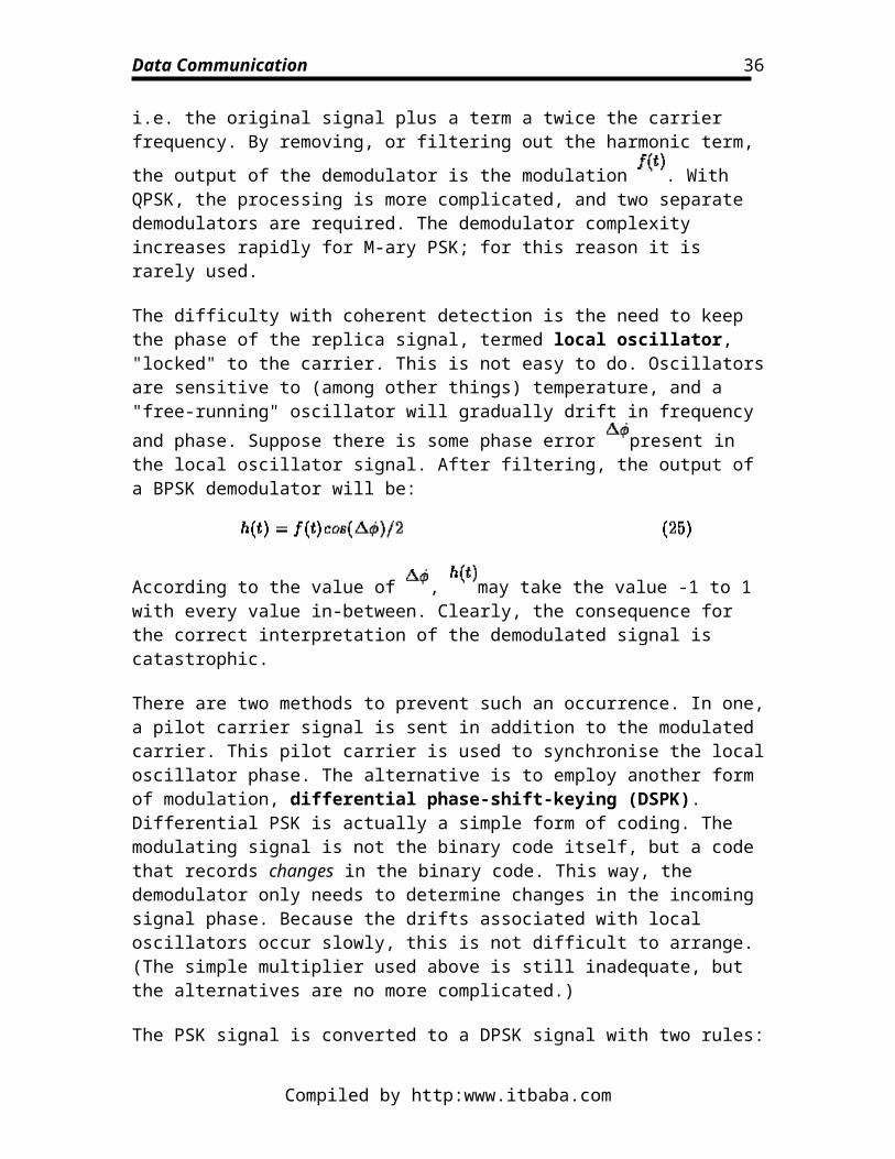
The difficulty with coherent detection is the need to keep the phase of the replica signal, termed local oscillator, "locked" to the carrier. This is not easy to do. Oscillators are sensitive to (among other things) temperature, and a "free-running" oscillator will gradually drift in frequency and phase. Suppose there is some phase error present in the local oscillator signal. After filtering, the output of a BPSK demodulator will be:


27

Data Communication

According to the value of , may take the value -1 to 1 with every value in-between. Clearly, the consequence for the correct interpretation of the demodulated signal is catastrophic.

There are two methods to prevent such an occurrence. In one, a pilot carrier signal is sent in addition to the modulated carrier. This pilot carrier is used to synchronise the local oscillator phase. The alternative is to employ another form of modulation, differential phase-shift-keying (DSPK). Differential PSK is actually a simple form of coding. The modulating signal is not the binary code itself, but a code that records changes in the binary code. This way, the demodulator only needs to determine changes in the incoming signal phase. Because the drifts associated with local oscillators occur slowly, this is not difficult to arrange. (The simple multiplier used above is still inadequate, but the alternatives are no more complicated.)

The PSK signal is converted to a DPSK signal with two rules:

1. a 1 in the PSK signal is denoted by no change in the DPSK 2. a 0 in the PSK signal is denoted by a change in the DPSK signal

The sequence is initialised with a leading 1. An example of the pattern is thus:

PSK 0 1 0 0 1 1 0 1 DPSK 1 0 0 1 0 0 0 1 1

Coherent detection is also necessary for the correct demodulation of narrow-band FSK. We have already noted that the form of the modulation signal gives rise to a bandwidth that is larger than that required by the Nyquist limit, and that has appreciable energy outside this bandwidth. This is in part due to the abrupt changes in the phase of the signal in FSK and PSK. By combining coherent detection with appropriate smoothing of the phase change, narrow-band FSK can become very bandwidth efficient, approaching the Nyquist limit, and have low side-lobe levels. This form of modulation, which is a combination of FSK and PSK, is termed minimum-shift-keying (MSK), or fast-FSK (FFSK).

To illustrate the way in which the complexity of demodulation determines the method used we consider two examples.

The modem is used to connect computer equipment to the PSTN to communicate with other equipment. The PSTN has a pass-band from 400Hz to 3400Hz; its bandwidth is 3000 Hz. Modems must be inexpensive if they are to be widely available. Variations in amplitude are common on telephone lines (don't we know it!) and ASK is not suitable. Incoherent FSK is widely used for low-rate modems. In all, four frequencies are used, two to transmit and two to receive. The bandwidth available per frequency is 750Hz, and with some simple smoothing baud rates up to 1200 baud are possible. For rates above this value PSK is necessary, and rates up to 2400 baud are possible.


28

Data Communication

For the second example, consider the problem of modulation choice for the down-link of a satellite microwave link. Here the requirement is for maximum data-rate, coupled with the need to avoid saturation of the available bandwidths close to the link bandwidth. In this case, MSK would be used, due to its good side-lobe performance and low bandwidth use. The additional cost of the demodulation processor is immaterial in comparison with the cost of the satellite.

Noise in communication systems; probability and random signalsNoise plays a crucial role in communication systems. In theory, it determines the theoretical capacity of the channel. In practise it determines the number of errors occurring in a digital communication. We shall consider how the noise determines the error rates in the next subsection. In this subsection we shall provide a description of noise.

Noise is a random signal. By this we mean that we cannot predict its value. We can only make statements about the probability of it taking a particular value, or range of values.

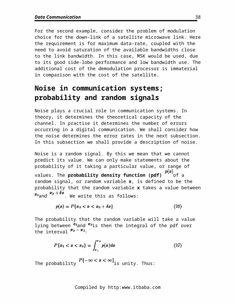
The probability density function (pdf) of a random signal, or random variable x, is defined to be the probability that the random variable x takes a value between and

. We write this as follows:

The probability that the random variable will take a value lying between and is then the integral of the pdf over the interval :

The probability is unity. Thus:

A density satisfying equation is termed normalised.

The probability distribution function is defined to be the probability that a random variable, x is less than :


29

http://www.cs.ucl.ac.uk/staff/S.Bhatti/D51-notes/node15.html#equpDense3

Data Communication

From the rules of integration:

Also, from equations and :

The meaning of the two functions and become clearer with the aid of examples.

Continuous distribution. An example of a continuous distribution is the Normal, or Gaussian distribution:

where m is the mean value of . The constant term ensures that the distribution is normalised. This expression is important as many naturally occurring noise sources can be described by it, e.g. white noise. Further, we can simplify the expression by considering the source to be a zero mean random variable, i.e. m = 0.

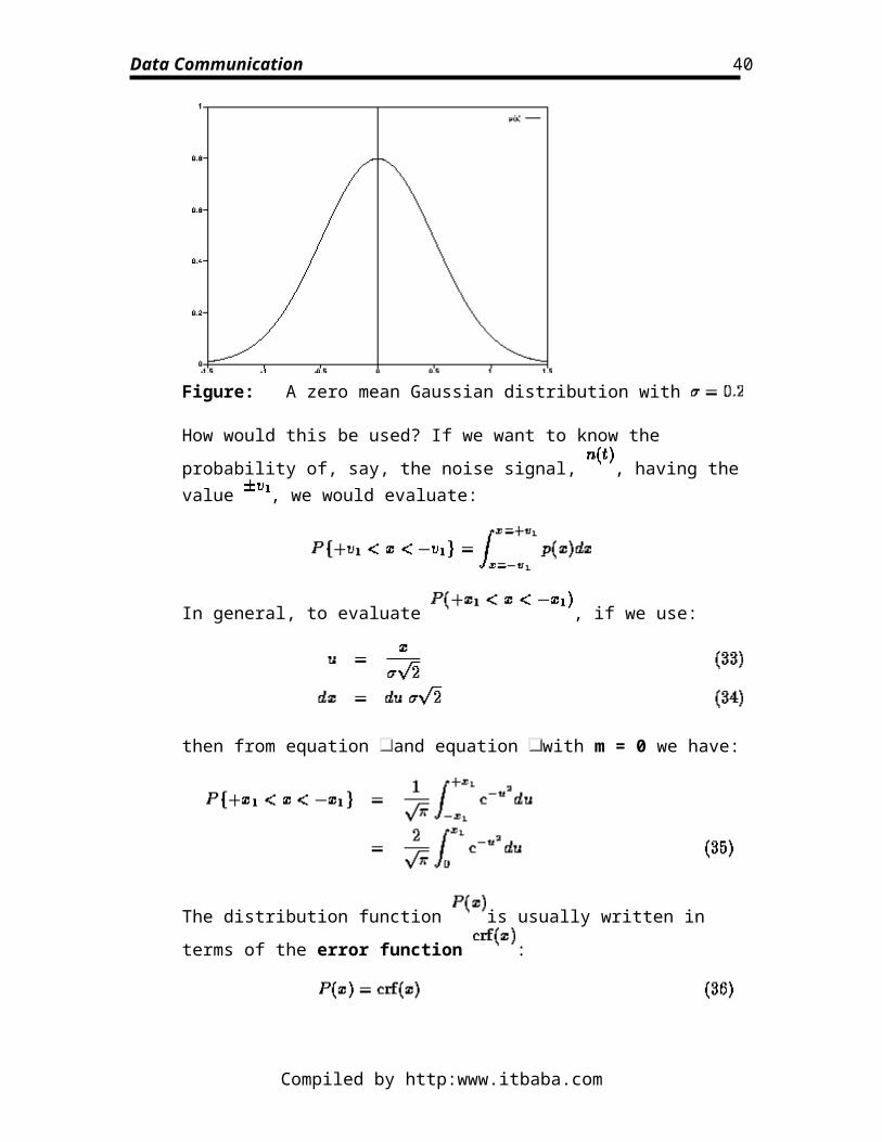
Figure: A zero mean Gaussian distribution with

How would this be used? If we want to know the probability of, say, the noise

signal, , having the value , we would evaluate:


30

http://www.cs.ucl.ac.uk/staff/S.Bhatti/D51-notes/node15.html#equpDense3

http://www.cs.ucl.ac.uk/staff/S.Bhatti/D51-notes/node15.html#equpDist1

Data Communication

In general, to evaluate , if we use:

then from equation and equation with m = 0 we have:

The distribution function is usually written in terms of the error function

:

where is given by:

which has the property:

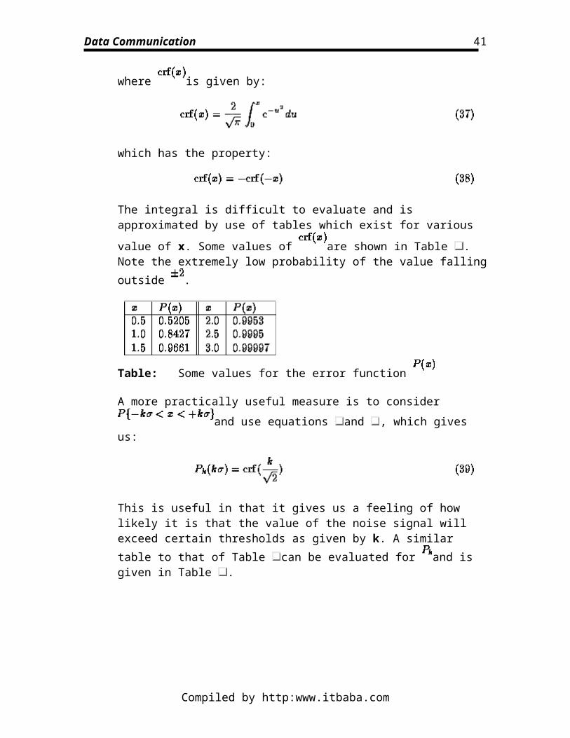
The integral is difficult to evaluate and is approximated by use of tables which

exist for various value of x. Some values of are shown in Table . Note the extremely low probability of the value falling outside .

Table: Some values for the error function

A more practically useful measure is to consider and use equations and , which gives us:


31

http://www.cs.ucl.ac.uk/staff/S.Bhatti/D51-notes/node15.html#equpDist1

http://www.cs.ucl.ac.uk/staff/S.Bhatti/D51-notes/node15.html#equGaussian

http://www.cs.ucl.ac.uk/staff/S.Bhatti/D51-notes/node15.html#tblerf

http://www.cs.ucl.ac.uk/staff/S.Bhatti/D51-notes/node15.html#equuerf

http://www.cs.ucl.ac.uk/staff/S.Bhatti/D51-notes/node15.html#equPerf

Data Communication

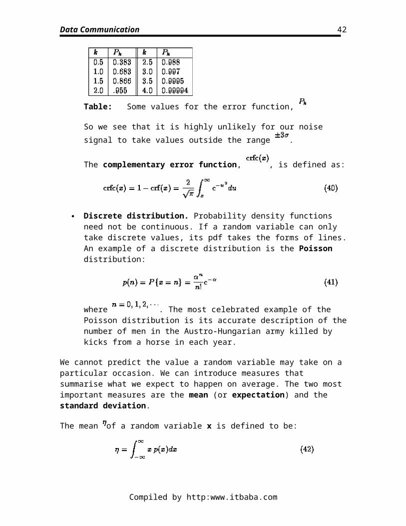
This is useful in that it gives us a feeling of how likely it is that the value of the noise signal will exceed certain thresholds as given by k. A similar table to that of Table can be evaluated for and is given in Table .

Table: Some values for the error function,

So we see that it is highly unlikely for our noise signal to take values outside the range .

The complementary error function, , is defined as:

Discrete distribution. Probability density functions need not be continuous. If a random variable can only take discrete values, its pdf takes the forms of lines. An example of a discrete distribution is the Poisson distribution:

where . The most celebrated example of the Poisson distribution is its accurate description of the number of men in the Austro-Hungarian army killed by kicks from a horse in each year.

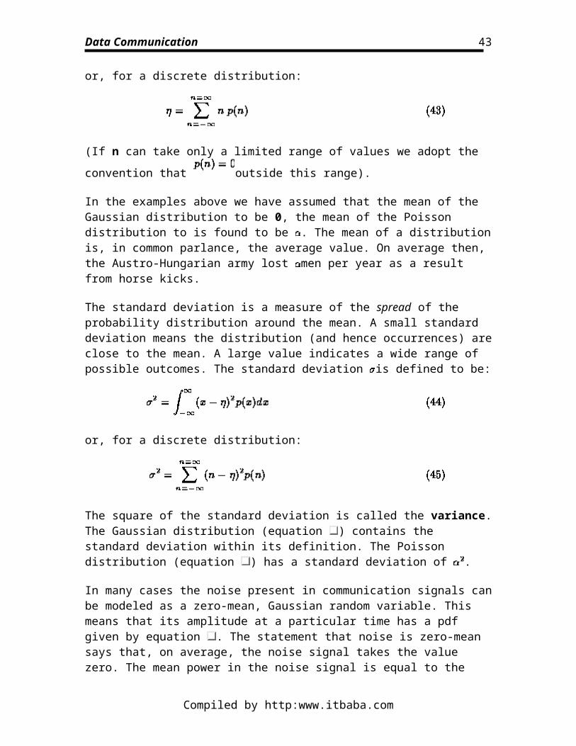
We cannot predict the value a random variable may take on a particular occasion. We can introduce measures that summarise what we expect to happen on average. The two most important measures are the mean (or expectation) and the standard deviation.

The mean of a random variable x is defined to be:

or, for a discrete distribution:


32

http://www.cs.ucl.ac.uk/staff/S.Bhatti/D51-notes/node15.html#tblerf

http://www.cs.ucl.ac.uk/staff/S.Bhatti/D51-notes/node15.html#tblkerf

Data Communication

(If n can take only a limited range of values we adopt the convention that outside this range).

In the examples above we have assumed that the mean of the Gaussian distribution to be 0, the mean of the Poisson distribution to is found to be . The mean of a distribution is, in common parlance, the average value. On average then, the Austro-Hungarian army lost men per year as a result from horse kicks.

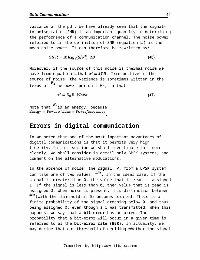
The standard deviation is a measure of the spread of the probability distribution around the mean. A small standard deviation means the distribution (and hence occurrences) are close to the mean. A large value indicates a wide range of possible outcomes. The standard deviation is defined to be:

or, for a discrete distribution:

The square of the standard deviation is called the variance. The Gaussian distribution (equation ) contains the standard deviation within its definition. The Poisson distribution (equation ) has a standard deviation of .

In many cases the noise present in communication signals can be modeled as a zero-mean, Gaussian random variable. This means that its amplitude at a particular time has a pdf given by equation . The statement that noise is zero-mean says that, on average, the noise signal takes the value zero. The mean power in the noise signal is equal to the variance of the pdf. We have already seen that the signal-to-noise ratio (SNR) is an important quantity in determining the performance of a communication channel. The noise power referred to in the definition of SNR (equation ) is the mean noise power. It can therefore be rewritten as:

Moreover, if the source of this noise is thermal noise we have from equation that . Irrespective of the source of noise, the variance is sometimes written in the

terms of the power per unit Hz, so that:


33


http://www.cs.ucl.ac.uk/staff/S.Bhatti/D51-notes/node15.html#equPoisson


http://www.cs.ucl.ac.uk/staff/S.Bhatti/D51-notes/node6.html#equSNR


Data Communication

Note that is an energy, because .

Errors in digital communicationIn we noted that one of the most important advantages of digital communications is that it permits very high fidelity. In this section we shall investigate this more closely. We shall consider in detail only BPSK systems, and comment on the alternative modulations.

In the absence of noise, the signal, V, from a BPSK system can take one of two values, . In the ideal case, if the signal is greater than 0, the value that is read is assigned 1. If

the signal is less than 0, then value that is read is assigned 0. When noise is present, this distinction between (with the threshold at 0) becomes blurred. There is a finite probability of the signal dropping below 0, and thus being assigned 0, even though a 1 was transmitted. When this happens, we say that a bit-error has occurred. The probability that a bit-error will occur in a given time is referred to as the bit-error rate (BER). In actuality, we may decide that our threshold of deciding whether the signal is

interpreted as a 0 or a 1 is set at such that any signal detected between a 0 is read if and a 1 is read if .

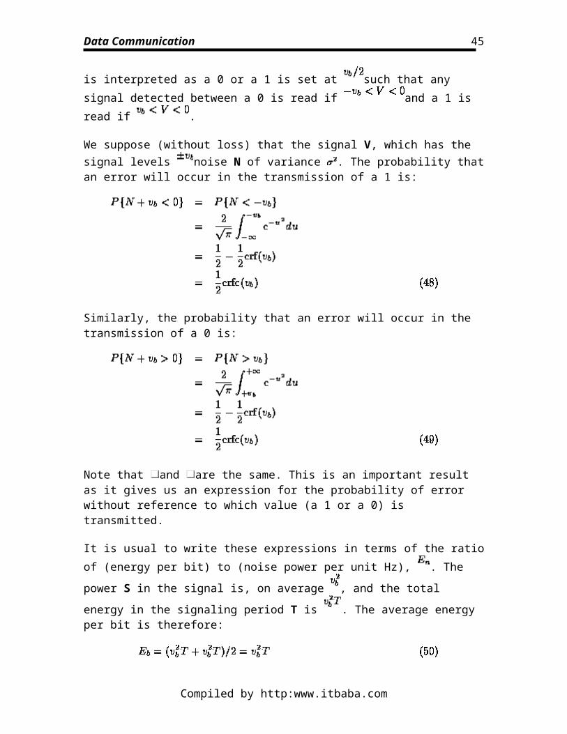
We suppose (without loss) that the signal V, which has the signal levels noise N of variance . The probability that an error will occur in the transmission of a 1 is:

Similarly, the probability that an error will occur in the transmission of a 0 is:

Note that and are the same. This is an important result as it gives us an expression for the probability of error without reference to which value (a 1 or a 0) is transmitted.


34

http://www.cs.ucl.ac.uk/staff/S.Bhatti/D51-notes/node16.html#equerror1


Data Communication

It is usual to write these expressions in terms of the ratio of (energy per bit) to (noise

power per unit Hz), . The power S in the signal is, on average , and the total energy

in the signaling period T is . The average energy per bit is therefore:

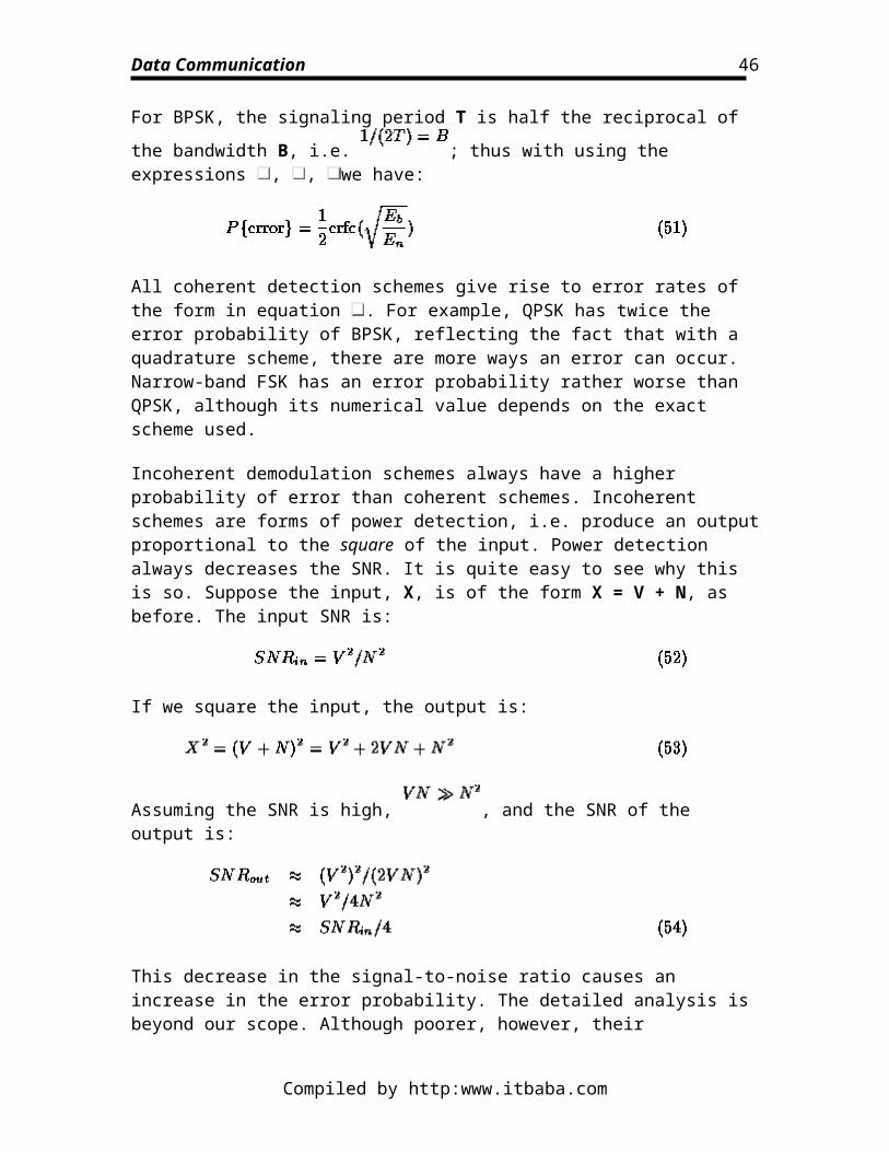
For BPSK, the signaling period T is half the reciprocal of the bandwidth B, i.e.

; thus with using the expressions , , we have:

All coherent detection schemes give rise to error rates of the form in equation . For example, QPSK has twice the error probability of BPSK, reflecting the fact that with a quadrature scheme, there are more ways an error can occur. Narrow-band FSK has an error probability rather worse than QPSK, although its numerical value depends on the exact scheme used.

Incoherent demodulation schemes always have a higher probability of error than coherent schemes. Incoherent schemes are forms of power detection, i.e. produce an output proportional to the square of the input. Power detection always decreases the SNR. It is quite easy to see why this is so. Suppose the input, X, is of the form X = V + N, as before. The input SNR is:

If we square the input, the output is:

Assuming the SNR is high, , and the SNR of the output is:

This decrease in the signal-to-noise ratio causes an increase in the error probability. The detailed analysis is beyond our scope. Although poorer, however, their performance is good nonetheless. This explains the widespread use of incoherent FSK.


35


http://www.cs.ucl.ac.uk/staff/S.Bhatti/D51-notes/node15.html#equnoiseEnergy

http://www.cs.ucl.ac.uk/staff/S.Bhatti/D51-notes/node16.html#equbitEnergy

http://www.cs.ucl.ac.uk/staff/S.Bhatti/D51-notes/node16.html#equerrorE

Data Communication

Error rates are usually quoted as bit error rates (BER). The conversion from error

probability to BER is numerically simple: BER = . However, this conversion assumes that the probabilities of errors from bit-to-bit are independent. This may or may not be a reasonable assumption. In particular, loss of timing can cause multiple bit failures that can dramatically increase the BER.

When signals travel along the channel, they are being attenuated. As the signal is losing power, the BER increases with the length of the channel. Regenerators, placed at regular intervals, can dramatically reduce the error rate over long channels. To determine the BER of the channel with N regenerators, it is simplest to calculate first the probability of no error. This probability is the probability of no error over one regenerator, raised to the Nth power:

assuming the regenerators are regularly spaced and the probabilities are independent. The BER is then determined simply by:

This avoids having to enumerate all the ways in which the multiple system can fail.

Timing control in digital communicationIn addition to providing the analogue modulation and demodulation functions, digital communication also requires timing control. Timing control is required to identify the rate at which bits are transmitted, and to identify the start and end of each bit. This permits the receiver to correctly identify each bit in the transmitted message. Bits are never sent individually. They are grouped together in segments, called blocks. A block is the minimum segment of data that can be sent with each transmission. (Usually, a message will contain many such blocks.) Each block is framed by binary characters identifying the start and end of the block. Sometimes, blocks are also referred to as frames. In addition to bit synchronisation, the receiver must also provide frame synchronisation, permitting the correct identification of the start and end of each block.

The type of method used depends on the source of the timing information. If the timing in the receiver is generated by the receiver, separately from the transmitter, the transmission is termed asynchronous. If the timing is generated, directly or indirectly, from the transmitter clock, the transmission is termed synchronous.

Asynchronous transmission is used for low data-rate transmission and stand-alone equipment. The block length is only 8 data-bits, permitting different clocks with only approximate synchronism to be used. Very commonly, the 8 bits represent an ASCII


36

Data Communication

character. For this reason, frame synchronisation is often referred to as character synchronisation in asynchronous systems.

Synchronous transmission is used for high data rate transmission. The timing is generated by sending a separate clock signal, or embedding the timing information into the transmission. This information is used to synchronise the receiver circuitry to the transmitter clock. Because the clocks are synchronised, much longer block lengths are possible.

The type of framing, character or block, is sometimes used to indicate whether a system uses asynchronous or synchronous transmission. This terminology does obscure the important difference between the different methods of timing control.

A typical asynchronous character frame consists of a start-bit, 8 data-bits and one or two stop bits. The start bit is chosen to have an opposite polarity to the line-idle state. Its arrival causes an idle/not-idle transition, that indicates to the receiver a character is arriving. The 8 data bits are then sampled (or clocked) through the receiver. The stop-bit(s) return the line to the idle state (Figure ).

Figure: Asynchronous character principle

The clocking is achieved by providing the receiver with a clock running several times faster than the bit-rate (Figure ). In this way, having identified the idle/start-bit transition, the receiver can easily identify the approximate centre of each bit. Because only 8 data-bits are transmitted, the clock need only be approximate; a 5% difference between transmitter and receiver clocks can be tolerated. (It should be recognised that with modern clock circuitry, a 5% error in clock rate is an enormous error.)

Figure: Asynchronous receiver operation with 8 clock

The addition of start and stop bits reduces the information rate of the channel. If one start and stop bit are used, the data-rate is 8/10 times the signaling rate. This is a general result. The addition of timing information always reduces the information rate of the channel.


37

http://www.cs.ucl.ac.uk/staff/S.Bhatti/D51-notes/node17.html#figasyncclock

http://www.cs.ucl.ac.uk/staff/S.Bhatti/D51-notes/node17.html#figasyncrxclock

Data Communication

Asynchronous transmission is used for transmissions up to 20Kb/s. When the data rate is high, the addition of framing characters around each byte becomes very inefficient. It is natural to wish to increase the block length, to maximise the data-rate. However, as the block length becomes longer, so errors in receiver clock rate less easy to tolerate, because they are accumulative. For example, if a 10000 bit frame is used, and we need to maintain the sampling point to within the central 50% of the bit period, the maximum clock rate error we can tolerate is 2.5 parts in . In consequence, asynchronous transmission is inappropriate for high data rates, and synchronous transmission must be used.

When using synchronous transmission, special procedures must be adopted to permit the unique identification of the frame. This is achieved by setting the frame header to a predetermined pattern. On transmission, any repeat of this pattern in the data is destroyed by the addition of binary zeroes, that are removed again on reception. This process is known as bit-stuffing.

Synchronous receivers require a timing signal from the transmitter. An additional channel may be used in the system to transmit the clock signal. This is wasteful of bandwidth, and it is more customary to embed the timing signal within the transmitted data stream by use of suitable encoding.

One way of embedding the timing signal is to encode the binary signal in such a way as to ensure a 1/0 transition with each bit. This transition is used to generate the clock signal used by the receiver. Bipolar encoding (Figure is an example of such a code. This uses a three level line; +V volts to represent a 1 and -V volts to represent a 0, and 0 volts between transmitting a 1 or 0. Bipolar encoding is an example of a return-to-zero (RZ) code.

Figure: Bipolar encoding

Another example of a timing code scheme is phase or Manchester encoding (Figure ). In this scheme, a transition in voltage level is used to represent a 1 or zero, rather than a voltage level itself, so only a two level line is needed. A 1 is represented by a low-high transition and 0 by a high-low transition. A transition occurs in the middle of each bit. This is an example of a non-return-to-zero (NRZ) code and requires a two level line.


38

http://www.cs.ucl.ac.uk/staff/S.Bhatti/D51-notes/node17.html#figbipolar

http://www.cs.ucl.ac.uk/staff/S.Bhatti/D51-notes/node17.html#figmanchester

Data Communication

Figure: Manchester encoding

These codes are very inefficient in their use of bandwidth. Both codes require a doubling of bandwidth over the original bit-stream, with no increase in data rate. RZ additionally requires a third signal level with no increase in data rate.

This increase can be avoided by using a device called a digital phase locked loop (DPLL). This uses a non-return-zero-inverted (NRZI) coding (Figure ). In NRZI, the signal is first NRZ encoded. Then, the NRZI signal is produced by the rule that a 1 in the NRZ signal produces no change in the NRZI signal, while a 0 in the NRZ signal produces a change in the NRZI signal. The details of the DPLL need not concern us. All we need to understand is that a DPLL has the property that, when presented with a timing signal, it can generate a second timing signal in synchronism with the first. This second signal is used to clock the data through the receiver. The DPLL has a settling time; the correct timing signal is not generated instantaneously. Conversely, the DPLL has "inertia"; it will continue to generate accurate timing after the "driving" signal has turned off. These properties permit the bit-stream itself to be used as a driver. On average, the bit stream will present sufficient 1/0 and 0/1 changes to ensure stable output from the DPLL. The practise of bit-stuffing often has the second function of ensuring sufficient 1/0 transitions for the DPLL. When using a DPLL, it is necessary to precede the frame with synchronisation characters whose only function is to permit the DPLL to settle before the start-frame bytes (or frame header) are read.

Figure: NRZI encoding for use with DPLL


39

http://www.cs.ucl.ac.uk/staff/S.Bhatti/D51-notes/node17.html#fignrzi

Data Communication

Design limitations on maximum data-rate and channel capacityIn the methods described in this section, we have found that the choice of modulation technique places a limit on the data rate. This limit is imposed by the number of levels in each signaling interval. For a binary system, there is two levels per signaling interval, and the maximum data-rate equals the signaling rate. We have also seen that the addition of framing and timing information will degrade the data-rate, so that in general, for a binary system, the data-rate will fall below the signaling rate. These limitations exist by virtue of practise, not principle; by introducing more complex circuitry and signal processing we may increase the data-rate.

An additional limitation on data-rate in some systems arises due to inter-symbol interference (ISI). ISI is the name given to the mistaken identification of one bit due to the presence of a bit in a neighboring time-slot (Figure ). The importance of ISI varies according to the system. Its effects can be reduced by signal processing, although simple techniques to perform this may require an increase in bandwidth. Its effects can dominate systems relying on crude incoherent detection. The data-rate of optical fibres is usually determined by the need to separate bit-intervals sufficiently to avoid ISI.

Figure: Intersymbol interference

Earlier, we introduced the Hartley-Shannon law that states that the maximum rate at which information can be transmitted error-free over a communication channel is the channel capacity C, given by equation :

For a given bandwidth, this relation states that as tends to infinity, so does the capacity. It is apparent that the methods we have just described will not satisfy this law. To take BPSK, for example, the maximum capacity in the absence of noise is equal to the signaling rate.

This inability to satisfy the Hartley-Shannon equation is often explained away by stating that it is a theoretical relation, and that we have to deal with the practical world. This is


40

http://www.cs.ucl.ac.uk/staff/S.Bhatti/D51-notes/node18.html#figisi


Data Communication

neither a good nor correct explanation. The law is valid for systems whose input and outputs may take any value. Since this is not true of our systems, the equation is not satisfied, but there is no reason why it should be. (We may derive an alternative relation for binary channels.) The remarkable feature of the Hartley-Shannon law is not that our channels do not obey it but that the message may be transmitted error-free. This is an astonishing result. If we consider our results of above we can see that, for a finite signal-to-noise ratio, we always have a finite probability of error. It is the existence of a channel capacity, not its functional form, that makes equation such an important relationship.

It is important to understand the distinction between maximum data-rate and capacity. The maximum data-rate is determined by the system design, and is associated with a given error rate. The channel capacity is the maximum rate that the channel can transmit data error-free, given its design. Clearly, the channel capacity cannot exceed the maximum-data rate. However, we have (as yet) said nothing concerning how error-free transmission might be achieved.

Communication channelsEarlier, we have described the terminology and general properties of communication channels. In this section, the properties of particular channels are described and contrasted. Broadly speaking, we may distinguish between channels that are physically connected with cable or fibre, and channels that have no physical connection, such as microwave links. Cable systems can be divided into transmission lines, that carry an electrical voltage between two conductors, and waveguides, that carry an electromagnetic wave.

Transmission lines Optical fibre waveguide The electromagnetic spectrum; propagation in free-space and the atmosphere;

noise in free-space Microwave link communication Satellite communication Optical fibre cables Mobile communications

Transmission linesA transmission line is a pair a conducting wires held apart by an insulator or dielectric. They come in a variety of construction geometries. The simplest and least expensive form


41










Data Communication

is two-wire (ribbon) cable. Twisted pair cable consists of two wires sheathed in an insulator and twisted together. Shielded pair cable contains two wires surrounded and separated by a solid dielectric. The dielectric is contained within a copper braid, that shields the conductors from external noise sources. The entire construction is housed in a flexible, waterproof cover.

The use of this kind of cable is limited by two factors: attenuation and cross-talk. There are three principle sources of attenuation. Resistance (or impedance) losses are simply the loss resulting from the resistance of the wires. This loss is minimised by the choice of a metal with low resistivity. Copper is chosen for this reason. (Gold is even better, and is in fact used on satellites to reduce losses.) Dielectric losses are caused by the heating effects when a varying electric field passes through a dielectric (insulator). Radiation losses occur because the cable acts as an antenna. All these losses increase with frequency.

Figure: Some different types of transmission lines

When a transmission line can act as an antenna, it can also act as a receiver. Lines prone to radiation loss are also susceptable to pick-up, or cross-talk. The first two types described above are particularly prone to this fault. The shielded pair is designed to reduce this pick-up.

All these lines have strong attenuation at frequencies above 1MHz. They are generally used for for low bit-rate communication. Two-wire ribbon cable is standard for the connection of individual telephone receivers. Twisted pair(s) is the normal method of connection for computer terminals and short high bit-rate connections.

Attenuation increases with both frequency and length. It is usually specified in dB/m at a particular frequency. Because of this fact, it is not possible to give hard-and-fast rules concerning the bandwidth availability of transmission lines. A twisted pair can support rates of several Mb/s over short distances (metres), but over long distances (kilometres) will be completely unsuitable at these data-rates.

For long distances, or data-rates in excess of several Mb/s, coaxial cable is used. Coaxial cable has a central wire, surrounded by a dielectric, in turn concentrically sheathed in a braided conductor. The cable is finally surrounded in a water-proof, flexible sheath. Coaxial cable is familiar to you -- it is the cable used to connect your television ariel. The


42

Data Communication

supreme advantage of this method of construction is its resistance to radiation losses. The outer conductor acts to shield out any external fields, whist preventing any internal fields escaping.

Until the advent of optical fibre, coaxial lines were the standard method of long-distance, high bit-rate communication. They are expensive (but getting cheaper, especially as demand rises), and only used where necessary. Typical attenuation values for coaxial cable are 10dB/Km at 10KHz, 50dB/Km at 500MHz. For very long-haul routes, repeaters and equalisers are necessary.

Figure: A sketch graph of attenuation in 0.375 inch coaxial cable

For short runs (metres), very high bit-rates are sustainable on coaxial cable -- up to 1Gb/s. At rates above this, the cables develop a waveguide action, and dispersion becomes a problem. Although it is possible to design coaxial cable that has still improved performance, these developments have been largely superceded by optical fibre.

Optical fibre waveguideFor many years it has been appreciated that the use of optical (light) waves as a carrier wave provides an enormous potential bandwidth. Optical carriers are in the region of Hz to Hz, i.e. three to six orders of magnitude higher than microwave frequencies. However, the atmosphere is a poor transmission medium for light waves. Optical communication only became a widespread option with the development of low-loss dielectric waveguide. In addition to the potential bandwidth, optical fibre communication offers a number of benefits:

Size, weight, flexibility. Optical fibres have very small diameters. A very large number of fibres can be carried in a cable the thickness of a coaxial cable.


43

Data Communication

Electrical isolation. Optical fibres are almost completely immune from external fields. They do not suffer from cross-talk, radio interference, etc.

Security. It is difficult to tap into an optical line. It is extremely difficult to tap into an optical line unnoticed.

Low transmission loss. Modern optical fibre now has better loss characteristics

than coaxial cable. Fibres have been fabricated with losses as low as .

The primary disadvantage of optical fibre are the technical difficulties associated with reliable and cheap connections, and the development of an optical circuit technology that can match the potential data-rates of the cables. The speed of these circuits, which are electronically controlled, is usually the limiting factor on the bit-rate. The difficulty of connection and high-cost of associated circuitry result in optical fibres being used only in very high bit-rate communication. There is considerable current debate as to whether optics will ever completely replace electronic technology. In addition, good phase control of an optical signal is extremely difficult. Optical communications are forced to use the comparatively crude method of ASK modulation.

Optical fibre is a waveguide. The fibre (in its simplest form) consists of a core of glass of one refractive index, and a cladding of a slightly lower refractive index (Figure ). The

fibre is then surrounded by a refractive sheath. Typical fibre dimensions are to

diameter.

Figure: The basic structure of a fibre optic waveguide

In simple terms, the action of a waveguide can be partially understood by considering the rays down the fibre. A light-wave entering the fibre is either refracted into the cladding, and attenuated, or is totally internally reflected at the core/cladding boundary. In this manner it travels along the length of the fibre. The maximum angle at which it may enter the guide and travel by total internal reflection is termed the acceptance angle (Figure ). It is also possible for the wave to follow a helical path down the guide. These rays are called skew-rays.


44

http://www.cs.ucl.ac.uk/staff/S.Bhatti/D51-notes/node21.html#figfibre

http://www.cs.ucl.ac.uk/staff/S.Bhatti/D51-notes/node21.html#figfibrewaveguide

Data Communication

Figure: Waveguide action of an optical fibre

However, this view is too simple to explain all features of waveguide behaviour. In fact, it is not possible for the wave to take any ray down the guide. Only certain rays can be taken. These rays are called modes. For any particular frequency, there is a different ray. The modal action of a waveguide is a consequence of the wave nature of the radiation. A mono-mode fibre is a fibre that only has one acceptable ray-path per frequency. A multi-mode fibre has a number of possible rays that light of a particular frequency may take.

The attenuation of light in the guide has a number of sources. Absorption of light occurs in the glass and this decreases with frequency. Scattering of light from internal imperfections within the glass -- Rayleigh scattering -- increases with frequency. Waveguide imperfections account for low-level loss that is approximately constant with wavelength. Bending the waveguide changes the local angle of total internal reflection and loss increases through the walls. A combination of these effects results in a minimum

absorption of about to in the to wavelength region. It is these wavelengths that are used for transmission. (See Figure .)


45

http://www.cs.ucl.ac.uk/staff/S.Bhatti/D51-notes/node21.html#figfibreloss

Data Communication

Figure: Sketch graph showing contributions to net spectral loss is a glass core

In addition to attenuation, optical waveguides also suffer from dispersion. The dispersion has two sources. Due to the modal behaviour, a waveguide is an intrinsically dispersive device. Put simply, rays of different frequency travel on different paths having different lengths. Because the different frequencies travel different lengths they take different times. In addition to the waveguide dispersion, however, is the material dispersion. Glass is an intrinsically dispersive media. In single mode fibres the material dispersion dominates the waveguide dispersion.

The bandwidth of optical fibres is dominated by the dispersion. In fact, the bandwidth of individual fibres is actually much the same as high quality co-axial cable. It is ironic that the principle justification for optical communication, very large bandwidth, has not in practise been realised. However, it is possible to lay many hundreds of optical fibres in the same cable cross-section as a single co-axial cable.

Fibre optic cable is available in three basic forms:

1. Stepped-index fibre. In this type of fibre, the core has a uniform refractive index

throughout. This generally has a core diameter of to . This is a multi-mode fibre. (Figure .)


46

http://www.cs.ucl.ac.uk/staff/S.Bhatti/D51-notes/node21.html#figsteppedindex

Data Communication

Figure: Stepped-index fibre

2. Graded-index fibre. In this type of fibre, the core has a refractive index that gradually decreases as the distance from the centre of the fibre increases. This

generally has a core diameter of . This is a multi-mode fibre. (Figure .)

Figure: Graded-index fibre

3. Mono-mode fibre. As the name suggests, the distinguishing characteristic of this fibre is that allows only a single ray path. The radius of the core of this type of fibre is much less than that of the other two, however it does have a uniform refractive index. (Figure .)

Figure: Mono-mode fibre

From, 1 to 3, we find that the cost of production increases, the complexity of transmitter and receiver increases, while the dispersion decreases. This latter property change means that the mono-fibre also has the potential to provide greater bandwidth. As it becomes cheaper to produce mono-mode fibre technology, we will see an increased use of this type of optical fibre. Figure gives typical operational information for a mono-mode fibre.


47

http://www.cs.ucl.ac.uk/staff/S.Bhatti/D51-notes/node21.html#figgradedindex

http://www.cs.ucl.ac.uk/staff/S.Bhatti/D51-notes/node21.html#figmonomode

http://www.cs.ucl.ac.uk/staff/S.Bhatti/D51-notes/node21.html#figmonomodefibre

Data Communication

Figure: Operational information for a mono-mode fibre

The electromagnetic spectrum; propagation in free-space and the atmosphere; noise in free-spaceIn this section we shall consider the physical properties of free-space electromagnetic waves, and how the atmosphere influences the propagation of electromagnetic waves. In the following sections, we shall describe how these properties have determined the selection of frequencies for communication.

The electromagnetic spectrum is divided up into a number of bands, as shown in Table .

Table: The higher frequencies of the electro-magnetic spectrum

Propagation of waves in free-space is different from that in cable or waveguides. With respect to signal propagation, these latter are one-dimensional systems, and a wave does not lose energy as it travels, except that due to absorption or scattering. In three-dimensions waves radiate spherically. As they travel, the surface area they occupy increases as the square of the distance traveled. However, since energy is conserved, the energy per unit surface area must decrease as the square of the distance. Thus the power of free-space waves obey an inverse square law. For each doubling of the distance between the source and receiver, a 6dB loss is experienced. For all frequencies up to


48

http://www.cs.ucl.ac.uk/staff/S.Bhatti/D51-notes/node22.html#tblspectrum

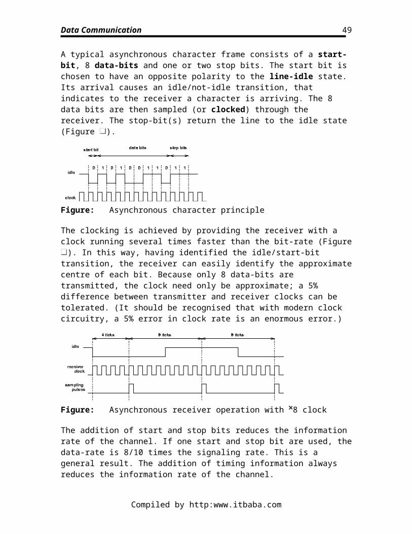
Data Communication

millimetre-wave frequencies, this free-space loss is the most important source of loss. Because of it, free-space systems usually require much more power than cable or fibre systems.

When waves traveling in free-space are obstructed, new waves result from the interaction. There are four types of interaction:

1. Reflection. This occurs when a wave meets a plane object. The wave is reflected back without distortion.

Figure: Reflection, refraction and diffraction

2. Refraction. This occurs when a wave encounters a medium with a different wave speed. The direction and speed of the wave is altered.

3. Diffraction. This occurs when the wave encounters an edge. The wave has the ability to turn the corner of the edge. This ability of waves to turn corners is called diffraction. It is markedly dependent on frequency -- the higher the frequency, the less diffraction. Very high frequencies (light) hardly diffract at all; "light travels in straight lines."

4. Scattering. Catch-all description of wave interactions that are too complex to be described as reflection, refraction or diffraction. Typically the result of scattering is to remove radiation of the wave, and re-radiate it over a wide range of directions. Scattering too is strongly frequency dependent. Usually it will increase with frequency.

Figure depicts reflection, refraction and diffraction of an electromagnetic wave.

The propagation of electromagnetic waves through the atmosphere is strongly influenced by the atmosphere (Figure ). From the point of view of wave propagation, there are two layers. The troposphere is the lowest layer of the atmosphere. It extends (typically) from the surface to a height of 50 Km. It contains all the Earth's weather, all the liquid water, most of the water vapour, most of the gaseous atmosphere, and most of the pollution. The ionosphere extends from the top of the troposphere into outer space. The ionosphere plays a crucial historical role in radio communication. It consists of oxygen molecules that are ionised by the action of the sun. During the day, the quantity of ions rises. At night, the ions recombine to form uncharged oxygen molecules. The ionisation of the atmosphere converts the ionosphere into a plasma: an electrically neutral gas of positive and negative charges.


49

http://www.cs.ucl.ac.uk/staff/S.Bhatti/D51-notes/node22.html#figrrd

http://www.cs.ucl.ac.uk/staff/S.Bhatti/D51-notes/node22.html#figemloss

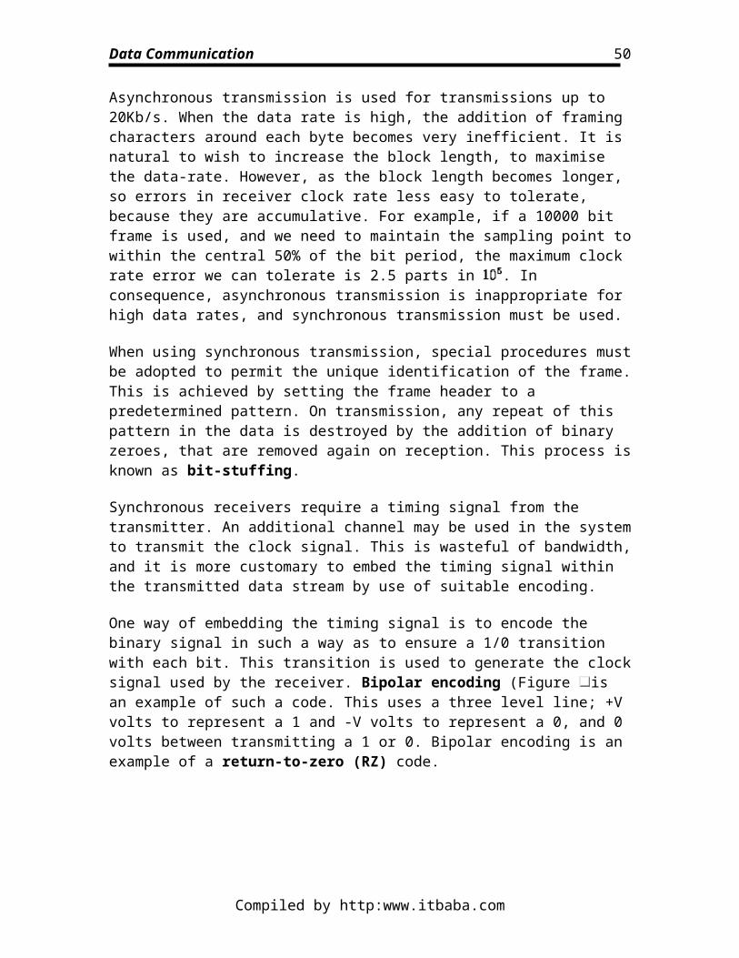
Data Communication

Figure: Sketch graph of attenuation due to rain, mist, water vapour and oxygen (temperate climate at ground level)

A plasma has a wave-speed that is a strong function of frequency. The consequence of this is that, to a low frequency wave, the ionosphere behaves as a mirror. Waves are simply reflected. This permits a mode of propagation in which the wave bounces forwards and backwards between the ionosphere and the Earth (Figure ). It was this mode of propagation that permitted Marconi, against the experts' advice, to achieve cross-Atlantic radio communication, and, in the process, discover the ionosphere. The Earth itself also acts as a mirror for electromagnetic waves. As the frequency increases to around 50MHz, the ionospheric effect reduces, and at higher frequencies becomes invisible.

Figure: Using the ionosphere for radiowave propagation

High Frequency (HF) propagation. The propagation of HF consists of two waves. The sky-wave, that bounces from the ionosphere, and the ground-wave, that propagates along the ground. Because of the long wavelengths, HF communications are not effected by the troposhpere, and can usually bend around even large objects such as hills. The ionosphere permits communication over great distances: these are the frequencies of the radio ham. The ionosphere is not dependable, however, and signal strengths can vary


50

http://www.cs.ucl.ac.uk/staff/S.Bhatti/D51-notes/node22.html#figionosphere

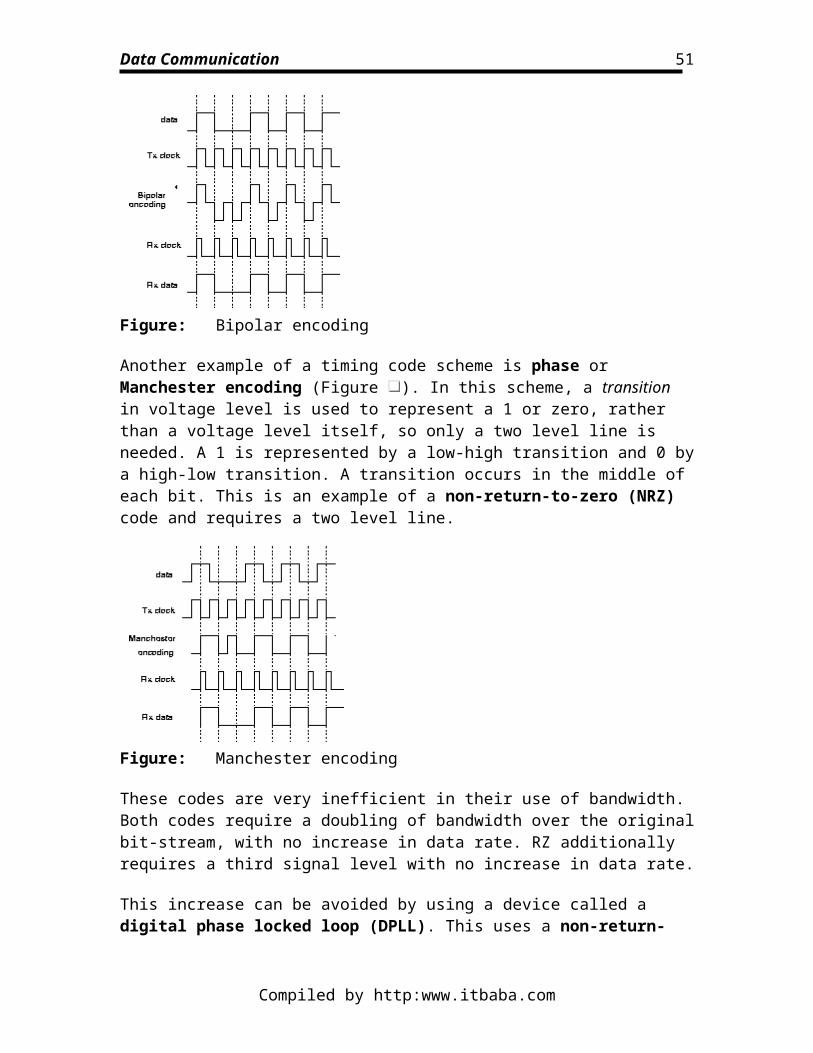
Data Communication

considerably -- effect is maximum in early evening, explaining the overcrowding of the medium wave-band in Britain with European transmissions in the evening.

Very High Frequency (VHF) and Ultra High Frequency (UHF) propagation. These frequencies are not effected by the troposphere, but are too high to exploit the ionosphere. In addition their decreased wavelength makes them increasingly less able to diffract around obstacles. At UHF in particular, areas in deep radio shadow can experience very poor reception. In urban areas, most reception is due to scattered arrivals. Experiments have shown that the free-space loss is increased in urban areas, to the extent of following a fourth power law. These effects are noticeable under motorway bridges: medium wavelength transmission is usually better than VHF. VHF is used for FM radio stations and UHF for TV transmissions.

When the received signal consists of a number of scattered arrivals, an effect called fading occurs. According to the location, the many arrivals may interfere constructively or destructively. The phase relationship between the arrivals changes as the location of receiver changes. This causes a moving receiver to experience fluctuations between strong and weak signals. This effect is known as fading.

Microwave and millimetre wave propagation. Microwave frequencies are usually completely blocked by obstructions. They need line-of-sight geometries. In addition, the wavelengths are small enough to become effected by water vapour and rain. Above 10GHz these effects become important. Above 25GHz, the effects of individual molecules becomes important. Water and oxygen are the most important gases. These have resonant absorption lines at 23, 69 and 120GHz (Figure ). Above these frequencies, absorption is increasingly effected by the Earth's black-body spectrum. These peaks leave "windows" that may be used for communication, notably at 38GHz and 98GHz.

Figure: Sketch graph of attenuation due to water and oxygen for microwave and millimetre wave


51

http://www.cs.ucl.ac.uk/staff/S.Bhatti/D51-notes/node22.html#figmmwaveloss

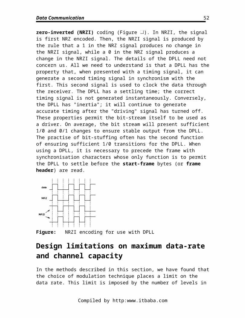
Data Communication

The use of the atmosphere as a transmission medium means that control over the noise environment is not possible. There are a number of sources of noise. Natural noise is classified by its source. Atmospheric noise dominates the low frequencies, up to 2MHz. The primary cause of this noise is electrical discharges in the atmosphere: lightning. So-called galactic noise is radio noise from outside the solar system. It is important up to 200GHz. The sun also generates a small noise contribution at these frequencies.

In urban environments these natural sources of noise are dominated by man-made noise. In the HF and VHF bands these are mostly other signals, although the very high power early warning radars can generate noise in these bands. At higher frequencies car ignition systems generate high noise levels. In comparison, receiver noise typically is small in the HF, UHF and VHF. At microwave frequencies, however, the thermal noise generated by the receiver (as given by equation ) is usually the dominant source of noise in the system.

Microwave link communicationThe maturity of radio frequency (RF) technology has permitted the use of microwave links as the major trunk channel for long distance communication. The use of microwave links has major advantages over cabling systems:

Freedom from land acquisition rights. The acquisition of rights to lay cabling, repair cabling, and have permanent access to repeater stations is a major cost in the provision of cable communications. The use of radio links, that require only the acquisition of the transmitter/receiver station, removes this requirement. It also simplifies the maintenance and repair of the link.

Ease of communication over difficult terrain. Some terrains make cable laying extremely difficult and expensive, even if the land acquisition cost is negligible.

The use of microwave links has a number of disadvantages, that mainly arise from the use of free-space communication:

Bandwidth allocation is extremely limited. The competition for RF bandwidth from various competing users leads to very strict allocations of bandwidth. Unlike cabling systems, that can increase bandwidth by laying more cables, the radio frequency (RF) bandwidth allocation is finite and limitied. In practise, bandwidth allocations of 50MHz in the carrier range 300MHz to 1GHz are typical.

Atmospheric effects. The use of free-space communication results in susceptibility to weather effects, particularly rain.

Transmission path needs to be clear. Microwave communication requires line-of-sight, point-to-point communication. The frequency of repeater stations is determined by the terrain. Care must be taken in the system design to ensure freedom from obstacles. In addition, links must be kept free of future constructions that could obstruct the link.

Interference. The microwave system is open to RF interference.


52


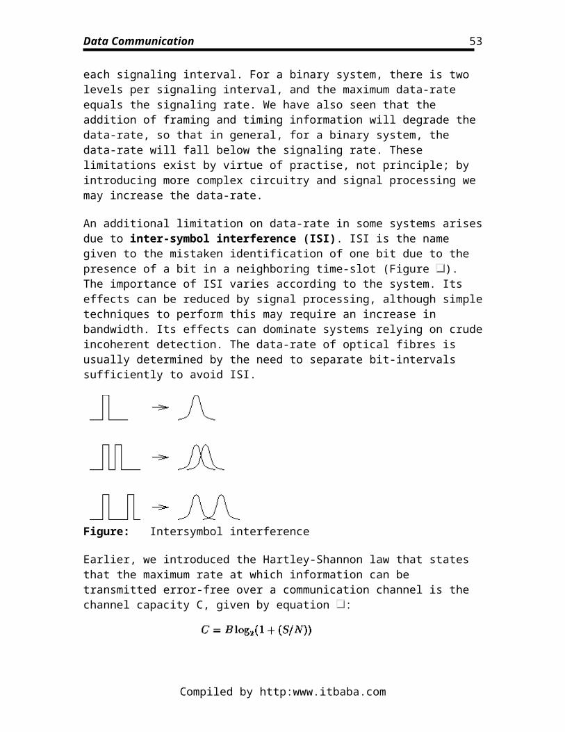
Data Communication

Restrictive Costs. The cost of design, implementation and maintenance of microwave links is high. Many countries are not well equipped with good technical resources to provide efficient and continuous operation.

The modern urban environment presents a particular challenge, in that bandwidth allocation, RF interference, link obstruction and atmospheric pollution place maximum constraints on the system simultaneously. However, urban environments also have the highest land acquisition values too. Many modern cities have found it cost effective to build a single, very high tower to house an entire city's trunk communication microwave dishes. These towers are now a common feature of the modern urban landscape.

As the demand for bandwidth increases, microwave links will become increasingly unable to deliver. The use of increased carrier frequencies in the millimetre wave region would be advantageous. However, for technical reasons, no efficient method of producing large quantities of millimetre power have been found. This is a necessity, given the increase in atmospheric attenuation at millimetre wave frequencies.

Satellite communicationSatellite communication became a possibility when it was realised (by the science fiction writer, Arthur C. Clarke) that a satellite orbiting at a distance of 36000Km from the Earth would be geostationary, i.e. would have an angular orbital velocity equal to the Earth's own orbital velocity. It would thus appear to remain stationary relative to the Earth if placed in an equatorial orbit. This is a consequence of Kepler's law that the period of rotation T of a satellite around the Earth was given by:

where r is the orbit radius, R is the Earth's radius and is the acceleration due to gravity at the Earth's surface. As the orbit increases in radius, the angular velocity reduces, until it is coincident with the Earth's at a radius of 36000Km. In principle, three geostationary satellites correctly placed can provide complete coverage of the Earth's surface (Figure ).


53

http://www.cs.ucl.ac.uk/staff/S.Bhatti/D51-notes/node24.html#figgeostationary

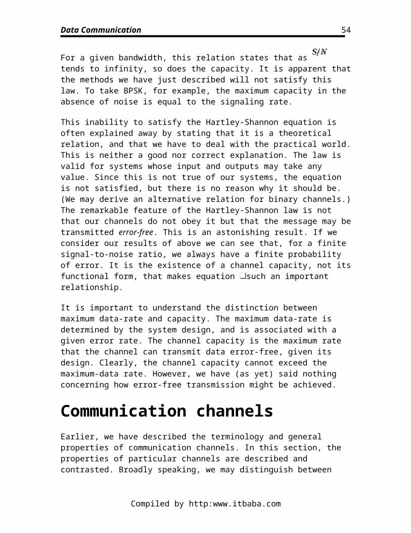
Data Communication

Figure: Geostationary satellites providing global coverage

For intercontinental communication, satellite radio links become a commercially attractive proposition. Space communication showed phenomenal growth in the 1970s, and will continue to grow for some years to come. The growth has been so rapid that there is now danger of overcrowding the geostationary orbit. Satellite communication has a number of advantages:

The laying and maintenance of intercontinental cable is difficult and expensive. The heavy usage of intercontinental traffic makes the satellite commercially

attractive. Satellites can cover large areas of the Earth. This is particularly useful for sparsely

populated areas.

Satellite communication is limited by four factors:

Technological limitations preventing the deployment of large, high gain antennas on the satellite platform.

Over-crowding of available bandwidths due to low antenna gains. The high investment cost and insurance cost associated with significant

probability of failure. High atmospheric losses above 30GHz limit carrier frequencies.

A microwave antenna has two functions. It provides gain (i.e. amplification). It also directs the radiation into confined regions of space: the antenna beam. These properties are largely dependent on the antenna size. For a circular, dish antenna, the gain G is related to the antenna area A by the formula:

where is the wavelength of the transmitted carrier. The angular width of the antenna beam is related to the antenna radius R by:


54

Data Communication

Thus, large antennas have high gains and narrow beams (Figure ).

Figure: A typical antenna beam profile of a dish antenna

The cost of constructing an antenna is a strong function of its size. A rough rule of thumb is the the cost is proportional to the diameter cubed. Thus a doubling of the antenna size will result in the satellite cost increasing eight times. As a result, antenna sizes are limited. The limitation in antenna size means that the satellite beam is wide. In order to prevent electromagnetic interference with terrestrial stations, the power radiated by the satellite is limited by international convention. In any event power is severely limited on a satellite platform.

Because the radiated power is low, large receiving antennas are required. The larger the receiver antenna, the larger the antenna gain, and hence the better the receiver SNR. The SNR is a function of the bandwidth, and the atmospheric attenuation. Ground stations close to the poles of the Earth have low elevation look angles, and signals have to pass through a thicker section of atmosphere. The size of receiver antenna is determined by

the two requirements; 500MHz receive bandwidth and full capability at of latitude.

A standard INTELSAT receiver is 30m in diameter. An antenna this large has a very narrow beam, typically . A geostationary satellite is not truly stationary, it wanders slightly in the sky. The very narrow beam width of the receiver requires automatic tracking of the satellite, and continuous pointing of the receiver antenna. An INTELSAT ground station is thus a large, expensive piece of equipment.

Satellite systems are extremely expensive. As an example, the break down for a particular British satellite is as shown in Table .


55

http://www.cs.ucl.ac.uk/staff/S.Bhatti/D51-notes/node24.html#figantennabeam

http://www.cs.ucl.ac.uk/staff/S.Bhatti/D51-notes/node24.html#tblsatPrice

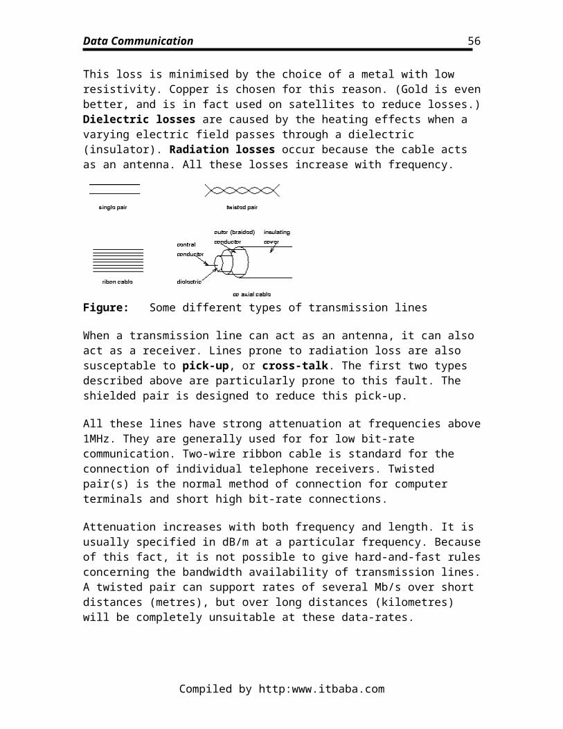
Data Communication

Table: Example costs for a satellite system

The use of satellites for regional communication is possible if there is sufficient demand

for traffic. By reducing the range of latitudes down to , and reducing the bandwidth down to 50MHz, large reductions in satellite and ground station receiver costs are possible. One such direct-to-user (DTU) system is the Satellite Business System (SBS) covering a range of business and governments users with a demand for high speed data links in the US. The region is split into areas, roughly coincident with the satellite antenna gain contours, denoting increased cost of receiver technology. It is important to realise that the economies of satellite communication only make this regional communication possible if the system is heavily used (Figure ).

Figure: The Satellite Business System operational schematic

Improvements in satellite receiver technology have permitted smaller antennas to be used as ground station receivers. However, antennas are reciprocal. They have the same directional characteristics in transmit and receive. The use of low gain, wide beam earth stations for DTU systems has contributed considerably to the bandwidth overcrowding problem, particularly in the US.


56

http://www.cs.ucl.ac.uk/staff/S.Bhatti/D51-notes/node24.html#figsatellitesystem

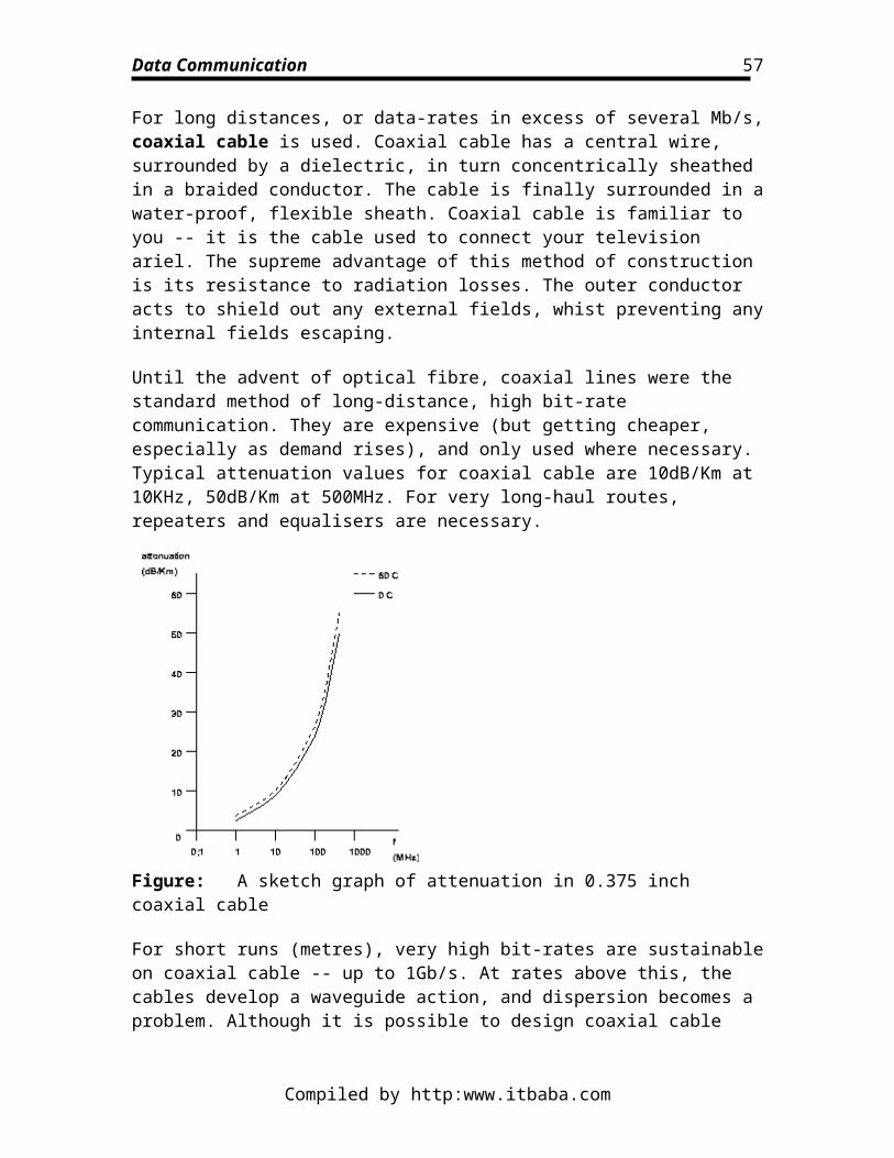
Data Communication

Recently there has been interest in low-earth orbiting (LEO) satellites. Here, a satellite placed in a 1000Km orbit has an orbital time of 1 hour. These satellites can be operated in a store-and-forward mode, picking up data at one part of the globe and physically transferring it to another. Because the data-rates and orbit radius are greatly reduced, small, low-cost satellites and ground stations are possible. However, such satellites have yet to demonstrate any commercial success.

Optical fibre cablesThe tremendous growth of optical fibre technology and its bandwidth capacity has led to a gradual replacement of microwave links with optical fibre cable for point-to-point communication. The rate of growth has depended on the communication policy of various nations. Europe has seen a rather more rapid growth than the US, reflecting the increased investment by government, however, there are many cable TV companies in the US that are laying fibre based networks. The primary disadvantage of optical cable is that it is largely restricted to point-to-point communications. Microwave and satellite systems retain an advantage in the ease with which they may be extended to include additional users.

Cable laying for intercontinental use is an expensive operation that, like satellites, can be justified only if the additional bandwidth is fully used. Optical fibre links now connect Britain and the US, and areas of Japan. Within the national network in Britain, the replacement of microwave systems by optical fibre is well advanced, especially in heavily populated areas of the country. Microwave systems will continue for some time to come, however, if only because they are already paid for. In addition, microwave links retain a considerable cost advantage in sparsely populated areas.

Mobile communicationsThe use of mobile radio-telephones has seen an enormous boost in the 1980s and 1990s. Previous to this time, citizen band (CB) radio had served a limited market. However, the bandwidth assignation for CB radio was very limited and rapidly saturated. Even in the U.S., a total of only 40 10KHz channels were available around 27MHz. The use of digital mobile telephones has a number of advantages over CB radio:

Access to national and international telephone system. Privacy of communication. Data independent transmission. An infinitely extendable number of channels.

Mobile communications are usually allocated bands in the 50MHz to 1GHz band. At these frequencies the effects of scattering and shadowing are significant. Lower frequencies would improve this performance, but HF bandwidth is not available for this purpose. The primary problems associated with mobile communication at these frequencies are:


57

Data Communication

Maintaining transmission in the fading circumstances of mobile communication. The extensive investigation of propagation characteristics required prior to

installation.

Mobile communication work by limiting transmitter powers. This restricts the range of communication to a small region. Outside this region, other transmitters can operated independently. Each region is termed a cell. These cells are often represented in diagrams as hexagons. In practise the cell shape is determined by local propagation characteristics. Together the cells will completely cover the area supplied with mobile communication coverage (Figures and ).

Figure: Use of cells to provide geographical coverage for mobile phone service

Figure: Frequency re-use in cells

Within each cell, the user communicates with a transmitter within the cell. As the mobile approaches a cell boundary, the signal strength fades, and the user is passed on to a transmitter from the new cell. Each cell is equipped with cell-site(s) that transmit/receive to/from the mobile within the cell. Within a single cell, a number of channels are available. These channels are (usually) separated by frequency. Then a mobile initiates a call, it is assigned an idle channel within the current cell by the mobile-services


58

http://www.cs.ucl.ac.uk/staff/S.Bhatti/D51-notes/node26.html#figcellcoverage

http://www.cs.ucl.ac.uk/staff/S.Bhatti/D51-notes/node26.html#figfreqreuse

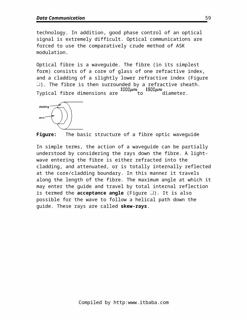
Data Communication

switching centre (MSC). He/she uses the channel within the cell until he/she reaches the boundary. He/she is then allocated a new idle channel within the next cell.

For example, the American advanced mobile phone service (AMPS) makes use of a 40MHz channel in the 800 - 900MHz band. This band is split into a 20MHz transmit and 20MHz receive bandwidth. These bands are split into 666 two-way channels, each having a bandwidth of 30KHz. These channels are subdivided into 21 sets of channels, arranged in 7 groups of 3. The nominally hexagonal pattern contains 7 cells, a central one and its 6 nearest neighbours. Each cell is assigned a different group in such a way that at least two cells lie between it and the next block using that set. With a total of 666 channels, it is possible to assign three sets of 31 channels per cell.

The great strength of this type of network is the ease with which more channels may be introduced. As demand rises, one simply reduces the cell size. Then the same number of channels is available in a smaller area, increasing the total number of channels per unit area. In a well planned system, the density of cells would reflect the user density.

AMPS is a first generation mobile phone system. It uses analogue modulation. It is one of six incompatible first generation systems that exist around the world. Currently, second generation systems are being introduced. These are digital in nature. One aim of the second generation mobile systems was to try and develop one global standard, allowing use of the same mobile phone anywhere in the world. However, there are are currently three digital standards in use, so this seems unlikely. The pan-European standard is known as GSM (Groupe Special Mobile), and is now available in the UK. The services planned for the GSM are similar to those for ISDN (e.g. call forwarding, charge advice, etc. ). Full GSM will have 200KHz physical channels offering 270Kb/s. Currently, one physical channel is split between 8 users, each having use of 13Kb/s (the rest is used for channel overhead). The aims of the GSM system were:

Good speech quality Low terminal cost Low service cost International roaming Ability to support hand-held portables A range of new services and facilities (ISDN!)

The heart of the mobile telephone network is the MSC. Its task is to acknowledge the paging of the user, assign him/her a channel, broadcast his/her dialed request, return the call. In addition it automatically monitors the signal strength of both transmitter and receiver, and allocates new channels as required. This latter process, known as hand-off, is completely hidden to the user, although is a major technical problem. In addition, the MSC is responsible for charging the call (Figure ). The decision making ability of the MSC relies to a great extent on modern digital technology. It is the maturity of this technology that has permitted the rapid growth of mobile communications.


59

http://www.cs.ucl.ac.uk/staff/S.Bhatti/D51-notes/node26.html#fighandoff

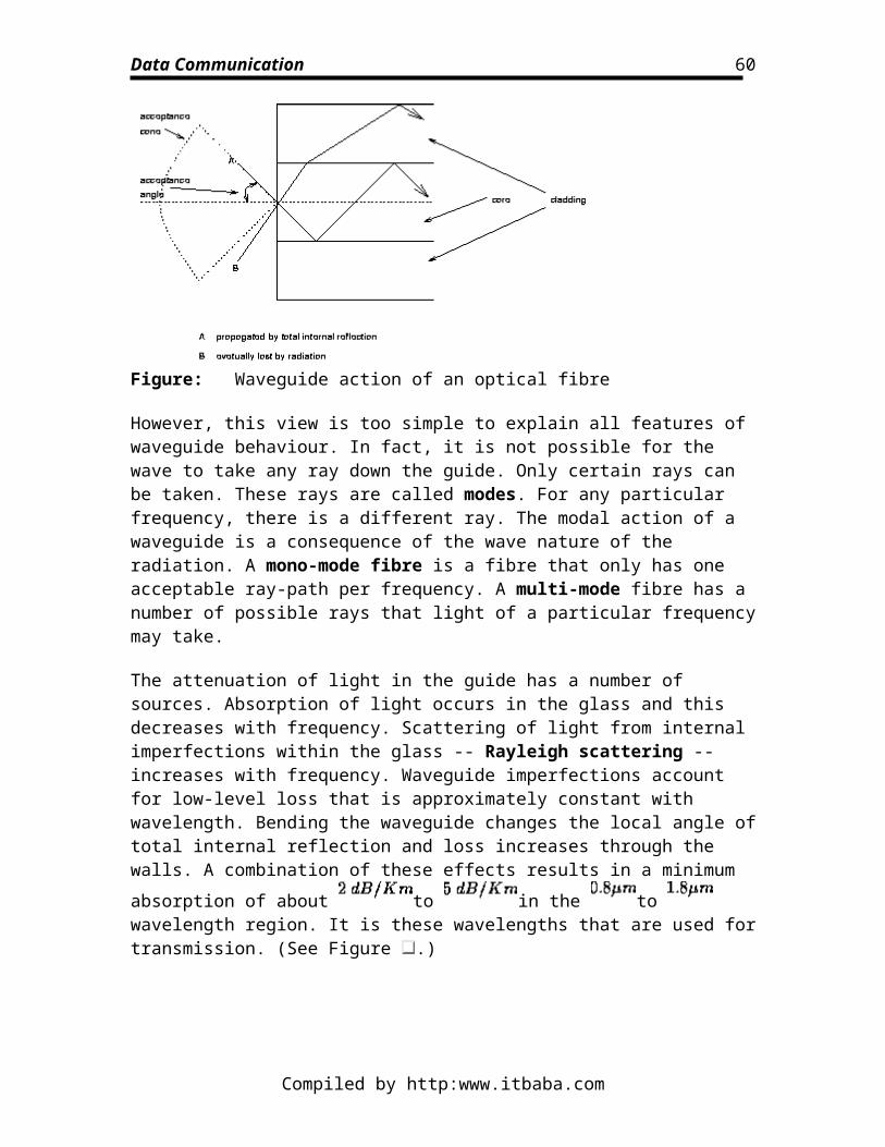
Data Communication

Figure: Hand-off between cells

The principle problem with mobile communication is the variation in signal strength as the communicating parties move. This variation is due to the varying interference of scattered radiation -- fading. Fading causes rapid variation in signal strength. The normal solution to fading, increasing the transmitter power, is not available in mobile communication where transmitter power is limited.

There is considerable research into suitable modulation schemes to cope with fading. The presence of fading has a severe effect on the BER. It can reduce the BER by several orders of magnitude over the non-fading case. In addition, some modulation schemes cope better than others. Surprisingly, coherent AM modulation is better than coherent FM in the fading environment. In any event BERs of are typical, in comparison with BERs of for non-fading channels. There should be no surprise if your mobile phone has a worse performance than that in your home.

The installation of a mobile telephone system requires a large initial effort in determining the propagation behaviour in the area covered by the network. Propagation planning, by a mixture of observation and computer simulation, is necessary if the system is to work properly. At UHF and VHF frequencies, the effects of obstructions is significant. Some of the effects that need to be considered are:

Free space loss. This significantly increases in urban environments. Studies have

indicated that a relationship is more often followed than a

law. Effect of street orientation. Streets have a significant waveguide effect.

Variations of up to 20dB have been measured in urban environments as a result of street direction.

Effects of foliage. Propagation in rural areas is significantly effected by the presence of leaves. Variations of 18dB between summer and winter have been observed in forested areas.

Effect of tunnels. Tunnels can introduce signal attenuation of up to 30dB according to the tunnel length and frequency.


60

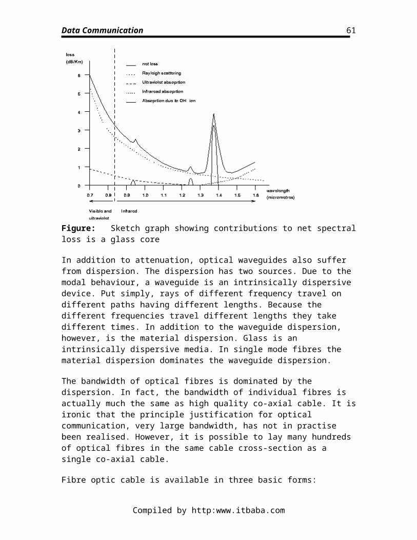
Data Communication

Information and Coding TheoryInformation theory is concerned with the description of information sources, the representation of the information from a source, and the transmission of this information over a channel.

Information Sources and Entropy Information source coding Channel coding; Hamming distance Channel capacity Error detection coding Error correction coding Encryption

Information Sources and EntropyConsider a rain forecast in the Sahara desert. This forecast is an information source. The information source has two outcomes: rain or no-rain. Clearly, the outcome no-rain contains little information; it is a highly probable outcome. The outcome rain, however, contains considerable information; it is a highly improbable event.

In information theory, an information source is a probability distribution, i.e. a set of probabilities assigned to a set of outcomes. This reflects the fact that the information contained in an outcome is determined not only by the outcome, but by how uncertain it is. An almost certain outcome contains little information.

A measure of the information contained in an outcome was introduced by Hartley in 1927. He defined the information (sometimes called self-information) contained in an outcome as:

This measure satisfies our requirement that the information contained in an outcome is

proportional to its uncertainty. If , then , telling us that a certain event contains no information.


61








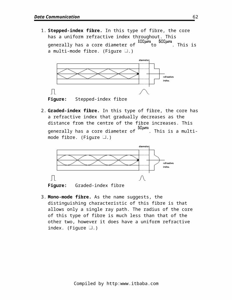
Data Communication

The definition also satisfies the requirement that the total information in independent events should add. Clearly, our rain forecast for two days contains twice as much information as for one day. From equation , for two independent outcomes and :

Hartley's measure defines the information in a single outcome. The measure entropy

, (sometimes absolute entropy), defines the information content of the source X as a whole. It is the mean information provided by the source per source output or symbol. We have from equation :

A binary symmetric source (BSS) is a source with two outputs whose probabilities are p and 1 - p respectively. The rain forecast discussed is a BSS. The entropy of the source is:

This (Figure ) function takes the value zero when p = 0. When one outcome is certain, so is the other, and the entropy is zero. As p increases, so too does the entropy, until it

reaches a maximum when . When p is greater than 1/2, the curve declines symmetrically to zero, reached when p = 1. We conclude that the average information in the BSS is maximised when both outcomes are equally likely. The entropy is measuring the average uncertainty of the source. (The term entropy is borrowed from thermodynamics. There too it is a measure of the uncertainty, or disorder of a system.)


62

http://www.cs.ucl.ac.uk/staff/S.Bhatti/D51-notes/node28.html#equHartley

http://www.cs.ucl.ac.uk/staff/S.Bhatti/D51-notes/node28.html#equHartley

http://www.cs.ucl.ac.uk/staff/S.Bhatti/D51-notes/node15.html#equPoissonmean

http://www.cs.ucl.ac.uk/staff/S.Bhatti/D51-notes/node28.html#figbss

Data Communication

Figure: Entropy of the binary symmetric source

When , . The unit of entropy is bits/symbol. An equally probable BSS has an entropy, or average information content per symbol, of 1 bit per symbol.

By long tradition, engineers have used the word bit to describe both the symbol, and its information content. A BSS whose outputs are 1 or 0 has an output we describe as a bit. The entropy of the source is also measured in bits, so that we might say the equi-probable

( ) BSS has an information rate of 1 bit/bit. The numerator bit refers to the information content. The denominator bit refers to the symbol 1 or 0. We can avoid this

by writing it as 1 bit/symbol. When , the BSS information rate falls. When

, bits/symbol. This means that, on average, each symbol (1 or 0) of source output is providing 0.47 bits of information.

For a BSS, the entropy is maximised when both outcomes are equally likely. This property is generally true. If an information source X has J symbols, its maximum

entropy is and this is obtained when all J outcomes are equally likely. Thus, for a J symbol source:

Information source codingIt seems intuitively reasonable that an information source of entropy H needs on average only H binary bits to represent each symbol. Indeed, the equi-probable BSS generates on average 1 information bit per symbol bit. However, consider the rain forecast again. Suppose the probability of rain is 0.1 and that of no-rain 0.9. We have already noted that this source has an entropy of 0.47 bits/symbol. Suppose we identify rain with 1 and no-


63

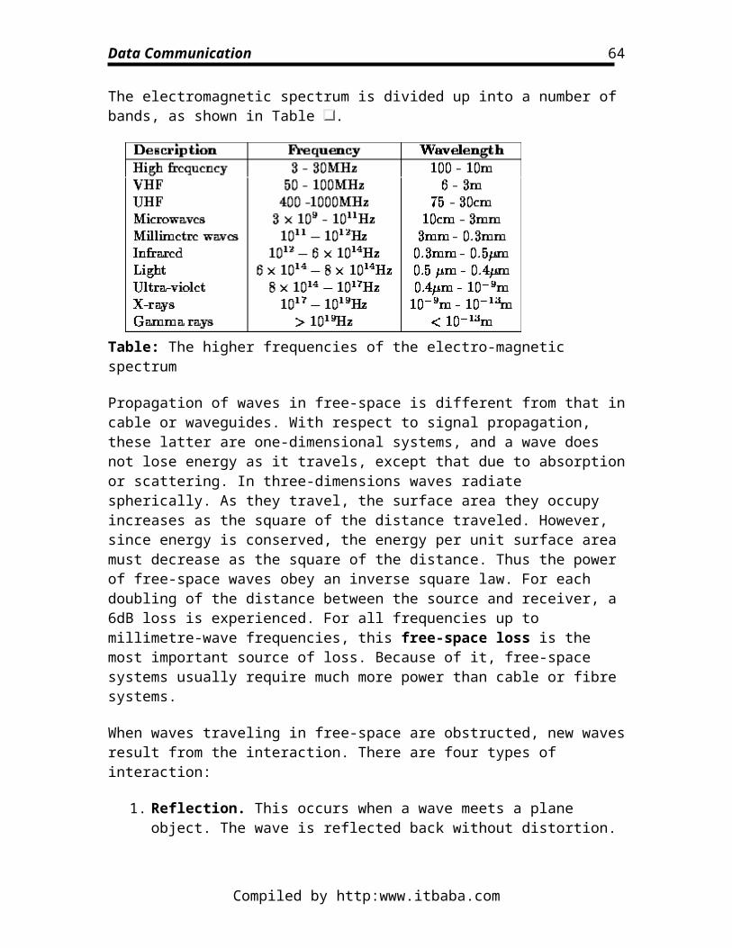
Data Communication

rain with zero. This representation uses 1 binary bit per symbol, and is using more binary bits per symbol than the entropy suggests is necessary.

The replacement of the symbols rain/no-rain with a binary representation is termed source coding. In any coding operation we replace the symbol with a codeword. The purpose of source coding is to reduce the number of bits required to convey the information provided by the information source.

Central to source coding is the use of sequences. By this, we mean that codewords are not simply associated to a single outcome, but to a sequence of outcomes. To see why this is useful, let us return to the problem of the rain forecast. Suppose we group the outcomes in threes, according to their probability, and assign binary codewords to these grouped outcomes. Table shows such a code, and the probability of each codeword occurring. It is easy to compute that this code will on average use 1.2 bits/sequence. Each sequence contains three symbols, so the code uses 0.4 bits/symbol.

This example shows how using sequences permits us to decrease the average number of bits per symbol. Moreover, without difficulty, we have found a code that has an average bit usage less than the source entropy. However, there is a difficulty with the code in Table . Before a codeword can be decoded, it must be parsed. Parsing describes the activity of breaking the message string into its component codewords. After parsing, each codeword can be decoded into its symbol sequence. An instantaneously parseable code is one that can be parsed as soon as the last bit of a codeword is received. An instantaneous code must satisfy the prefix condition. That is, no codeword may be a prefix of any other codeword. This condition is not satisfied by the code in Table .

The code in Table , however, is an instantaneously parseable code. It satisfies the prefix condition.

Table: Variable length coding


64

http://www.cs.ucl.ac.uk/staff/S.Bhatti/D51-notes/node29.html#tblvlc



http://www.cs.ucl.ac.uk/staff/S.Bhatti/D51-notes/node29.html#tblhuffman

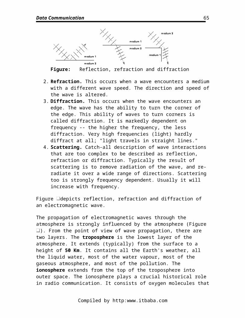
Data Communication

Table: Instantly parseable variable length coding

The code in Table uses on average 1.6 bits per sequence, or 0.53 bits/symbol. This is a 47% improvement on identifying each symbol with a bit. In fact this is the Huffman code for the sequence set. The code for each sequence is found by generating the Huffman code tree for the sequence. A Huffman code tree is an unbalanced binary tree. The derivation of the Huffman code tree is shown in Figure and the tree itself is shown in Figure . In both these figures, the letters A to H have been used in place of the sequences in Table to make them easier to read.

Figure: Example derivation of a Huffman code tree


65


http://www.cs.ucl.ac.uk/staff/S.Bhatti/D51-notes/node29.html#fighuffman1



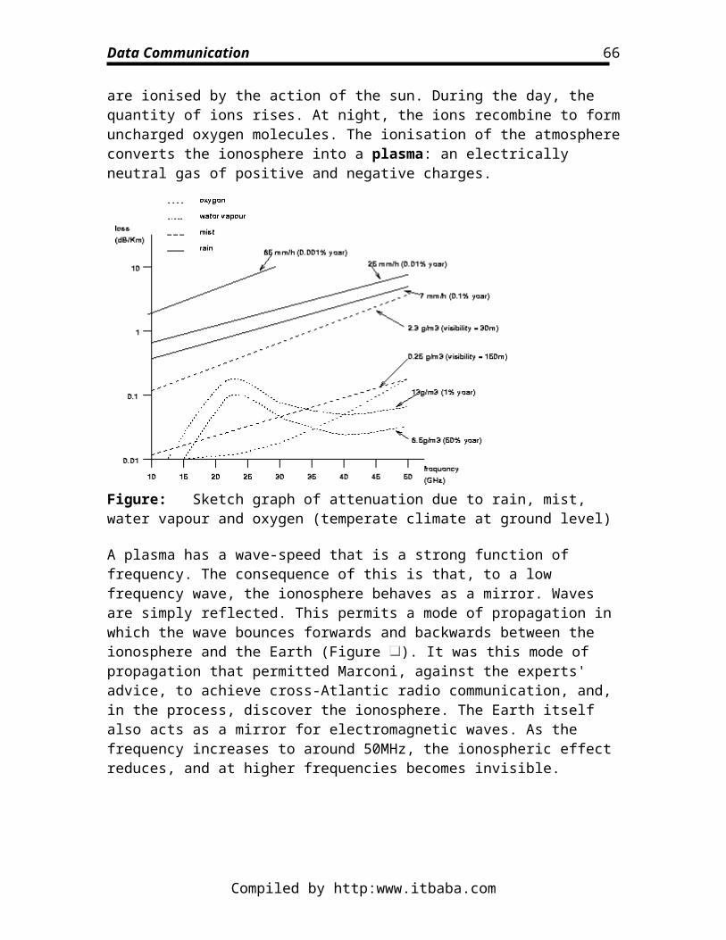
Data Communication

Figure: Example Huffman code tree

In Figure , the sequences are ordered with respect to the probability of the sequence occurring, highest probability at the top of the list. (The probabilities are effectiveley used as weights in the process to be described.) The tree is derived bottom up, in terms of branch nodes and leaf nodes by combining weights and removing leaf nodes in progressive stages. As shown in Figure , the two lowest leaf nodes G and H have their weights added, and the topmost node is labelled with a 1 and the lower one with a 0. In the next stage the are represented by that weight, and the list is rewritten, agan in order of the weights. The two lowest leaf nodes are now E and F, and they are labelled 1 and 0, respectiveley, and their weights are added to be taken on to the next stage. This continues until only two nodes remain. The Huffman tree shown in Figure is then produced by following backwards along the arrows in Figure . To derived the codewords from the tree, descend from the top node (the root node), and list the 1s and 0s in the order you appear until you reach the leaf node for one of the letters.

Huffman coding relies on the fact that both the transmitter and the receiver know the sequence set (or data set) before communicating and can build the code table. Where this is not possible dynamic Huffman coding can be used to build up the code table as the data is transmitted or received.

The noiseless source coding theorem (also called Shannon's first theorem) states that

an instantaneous code can be found that encodes a source of entropy with an average number of bits per symbol such that:

Ordinarily, the longer the sequences of symbols, the closer will be to .

Like many theorems of information theory, the theorem tells us nothing of how to find the code. However, it is a useful result. For example, the code in Table uses 0.53 bits/symbol which is only 11% more bits per symbol than the theorem tells us is the best we can do (0.47 bits/symbol). We might conclude that there is little point in expending the effort in finding a code closer to satisfying the inequality .


66






http://www.cs.ucl.ac.uk/staff/S.Bhatti/D51-notes/node29.html#equShannon

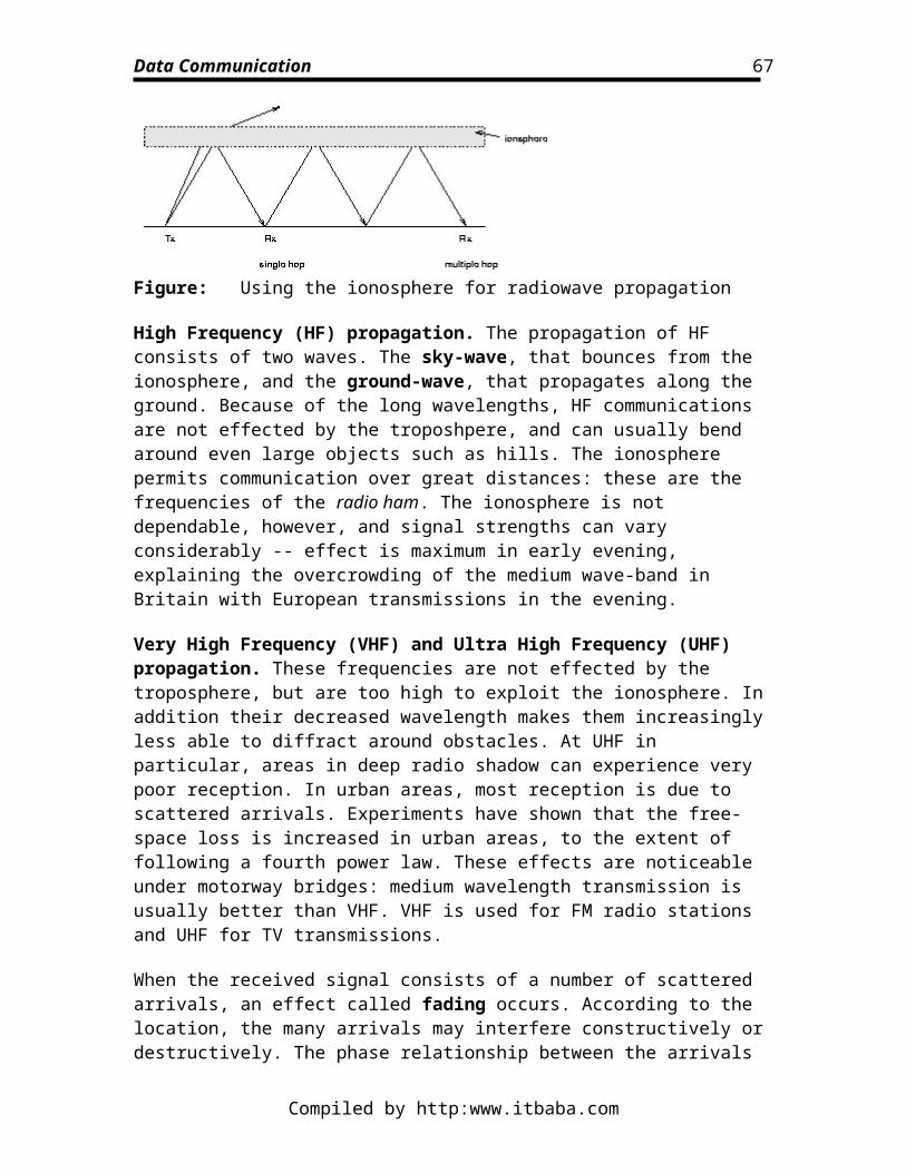
Data Communication

Channel coding; Hamming distanceThe task of source coding is to represent the source information with the minimum of symbols. When a code is transmitted over a channel in the presence of noise, errors will occur. The task of channel coding is to represent the source information in a manner that minimises the error probability in decoding.

It is apparent that channel coding requires the use of redundancy. If all possible outputs of the channel correspond uniquely to a source input, there is no possibility of detecting errors in the transmission. To detect, and possibly correct errors, the channel code sequence must be longer than the source sequence. The rate R of a channel code is the average ratio of the source sequence length to the channel code length. Thus, R < 1.

A good channel code is designed so that, if a few errors occur in transmission, the output can still be identified with the correct input. This is possible because although incorrect, the output is sufficiently similar to the input to be recognisable. The idea of similarity is made more firm by the definition of a Hamming distance. Let x and y be two binary sequences of the same length. The Hamming distance between these two codes is the number of symbols that disagree. Suppose the code x is transmitted over the channel. Due to errors, y is received. The decoder will assign to y the code x that minimises the Hamming distance between x and y. For example, consider the codewords:

a 10000 b 01100 c 10011

If the transmitter sends 10000 but there is a single bit error and the receiver gets 10001, it can be seen that the "nearest" codeword is in fact 10000 and so the correct codeword is found.

It can be shown that to detect n bit errors, a coding scheme requires the use of codewords with a Hamming distance of at least n + 1. It can also be shown that to correct n bit errors requires a coding scheme with at least a Hamming distnace of 2n + 1 between the codewords.

By designing a good code, we try to ensure that the Hamming distance between possible codewords x is larger than the Hamming distance arising from errors.

Channel capacityOne of the most famous of all results of information theory is Shannon's channel coding theorem. For a given channel there exists a code that will permit the error-free

transmission across the channel at a rate R, provided , the channel capacity. Equality is achieved only when the SNR is infinite.


67

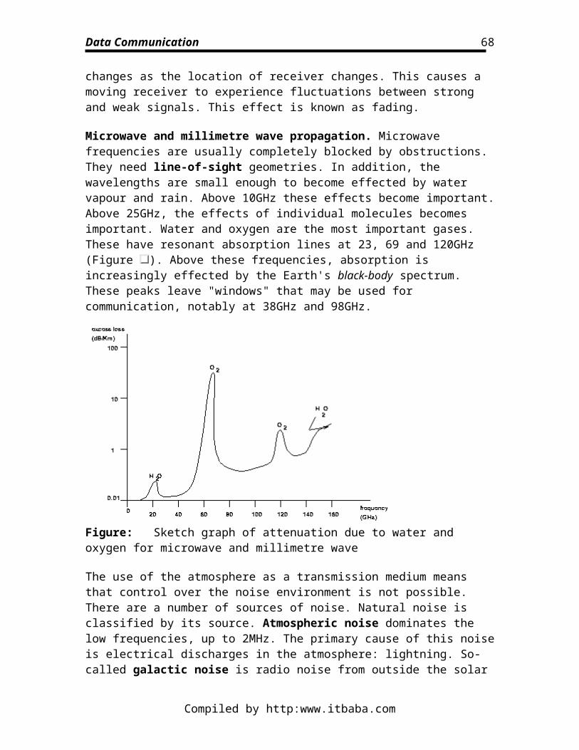
Data Communication

As we have already noted, the astonishing part of this theory is the existence of a channel capacity. Shannon's theorem is both tantalising and frustrating. It offers error-free transmission, but it makes no statement as to what code is required. In fact, all we may deduce from the proof of the theorem is that it must be a long one. No one has yet found a code that permits the use of a channel at its capacity. However, Shannon has thrown down the gauntlet, in as much as he has proved that the code exists.

We shall not give a description of how the capacity is calculated. However, an example is instructive. The binary channel (BC) is a channel with a binary input and output. Associated with each output is a probability p that the output is correct, and a probability

it is not. For such a channel, the channel capacity turns out to be:

Here (Figure ), p is the bit error probability. If p = 0 then C = 1. If the C = 0. Thus, if there is equal probability of receiving a 1 or 0, irrespective of the signal sent, the channel is completely unreliable and no message can be sent across it.

Figure: The capacity of a binary channel

So defined, the channel capacity is a non-dimensional number. We normally quote the capacity as a rate, in bits/second. To do this we relate each output to a change in the signal. For a channel of bandwidth B, we can transmit at most 2B changes per second. Thus, the capacity in bits/second is 2BC. For the binary channel, we have:

For the binary channel the maximum bit rate W is 2B. We note that C < W, i.e. the capacity is always less than the bit rate. The data rate D, or information rate describes the rate of transfer of data bits across the channel. In theory, we have:


68

http://www.cs.ucl.ac.uk/staff/S.Bhatti/D51-notes/node31.html#figbinarychannel

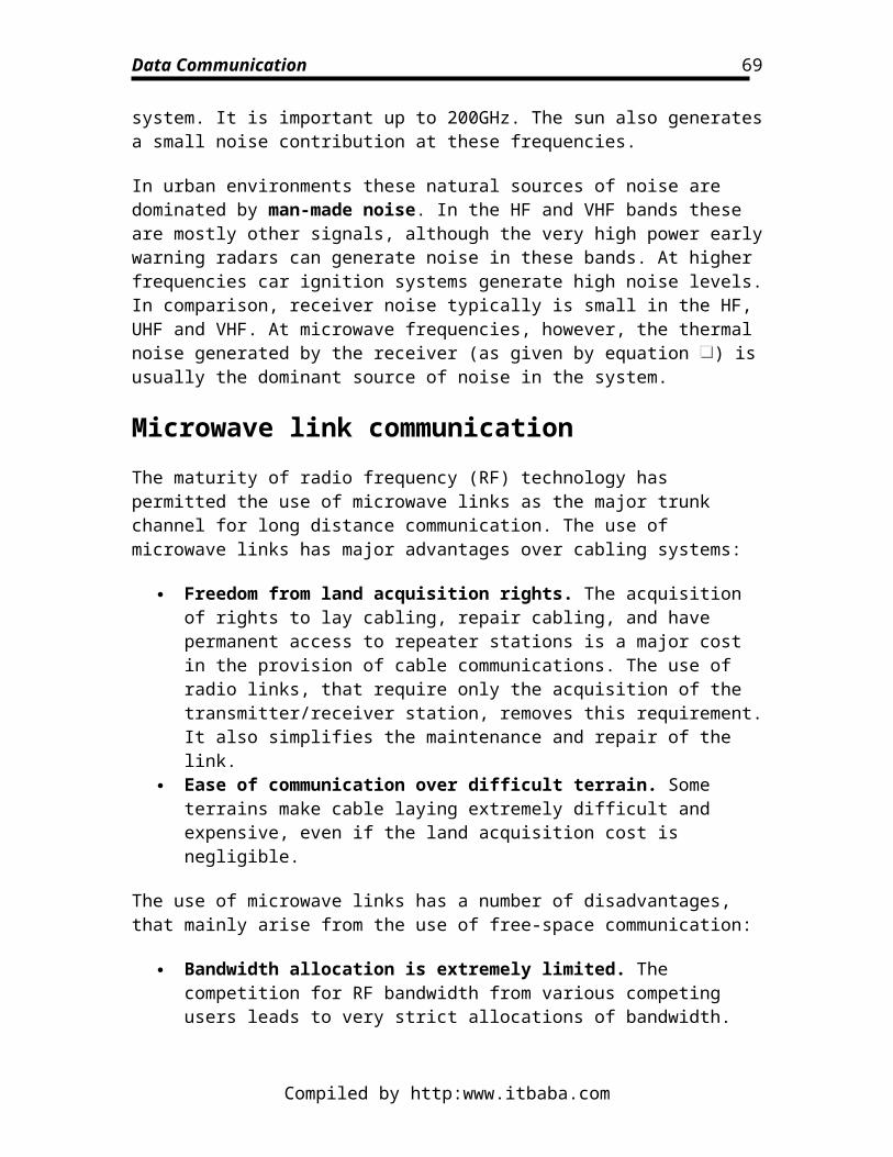
Data Communication

As a matter of practical fact:

Shannon's channel coding theorem applies to the channel, not to the source. If the source is optimally coded, we can rephrase the channel coding theorem: A source of information

with entropy can be transmitted error free over a channel provided .

All the modulations described earlier are binary channels. For equal BER, all these schemes have the same capacity. We have noted, however, that QPSK only uses half the bandwidth of PSK for the same bit rate. We might suppose that for the same bandwidth, QPSK would have twice the capacity. This is not so. We have noted that PSK modulation is far from optimum in terms of bandwidth use. QPSK makes better use of the bandwidth. The increase in bit rate provided by QPSK does not reflect an increase in capacity; merely a better use of bandwidth.

The capacity of the binary channel is much less than that calculated from the Hartley-Shannon Law (equation ). Why so? The answer is that equation applies to systems whose outputs may take any values. We use systems obeying equation because they are technically convenient, not because they are desirable.

Error detection codingThe theoretical limitations of coding are placed by the results of information theory. These results are frustrating in that they offer little clue as to how the coding should be performed. Error detection coding is designed to permit the detection of errors. Once detected, the receiver may ask for a re-transmission of the erroneous bits, or it may simply inform the recipient that the transmission was corrupted. In a binary channel, error checking codes are called parity check codes.

Practical codes are normally block codes. A block code converts a fixed length of K data

bits to a fixed length N codeword, where N > K. The rate of the code is the ratio ,

and the redundancy of the code is . Our ability to detect errors depends on the rate. A low rate has a high detection probability, but a high redundancy.

The receiver will assign to the received codeword the preassigned codeword that minimises the Hamming distance between the two words. If we wish to identify any pattern of n or less errors, the Hamming distance between the preassigned codewords must be n + 1 or greater.

A very common code is the single parity check code. This code appends to each K data bits an additional bit whose value is taken to make the K + 1 word even (or odd). Such a


69



http://www.cs.ucl.ac.uk/staff/S.Bhatti/D51-notes/node31.html#equbinaryChannel2

Data Communication

choice is said to have even (odd) parity. With even (odd) parity, a single bit error will make the received word odd (even). The preassigned code words are always even (odd), and hence are separated by a Hamming distance of 2 or more.

To see how the addition of a parity bit can improve error performance, consider the

following example. A common choice of K is eight. Suppose the BER is . Then:

So, the probability of a transmission with an error is . With the addition of a parity error bit we can detect any single bit error. So:

As can be seen, the addition of a parity bit has reduced the uncorrected error rate by three orders of magnitude.

Single parity bits are common in asynchronous, character oriented transmission. Where synchronous transmission is used, additional parity symbols are added that checks not only the parity of each 8 bit row, but also the parity of each 8 bit column. The column is formed by listing each successive 8 bit word one beneath the other. This type of parity checking is called block sum checking, and it can correct any single 2 bit error in the transmitted block of rows and columns. However, there are some combinations of errors that will go undetected in such a scheme (Figure )


70

http://www.cs.ucl.ac.uk/staff/S.Bhatti/D51-notes/node32.html#figbsc

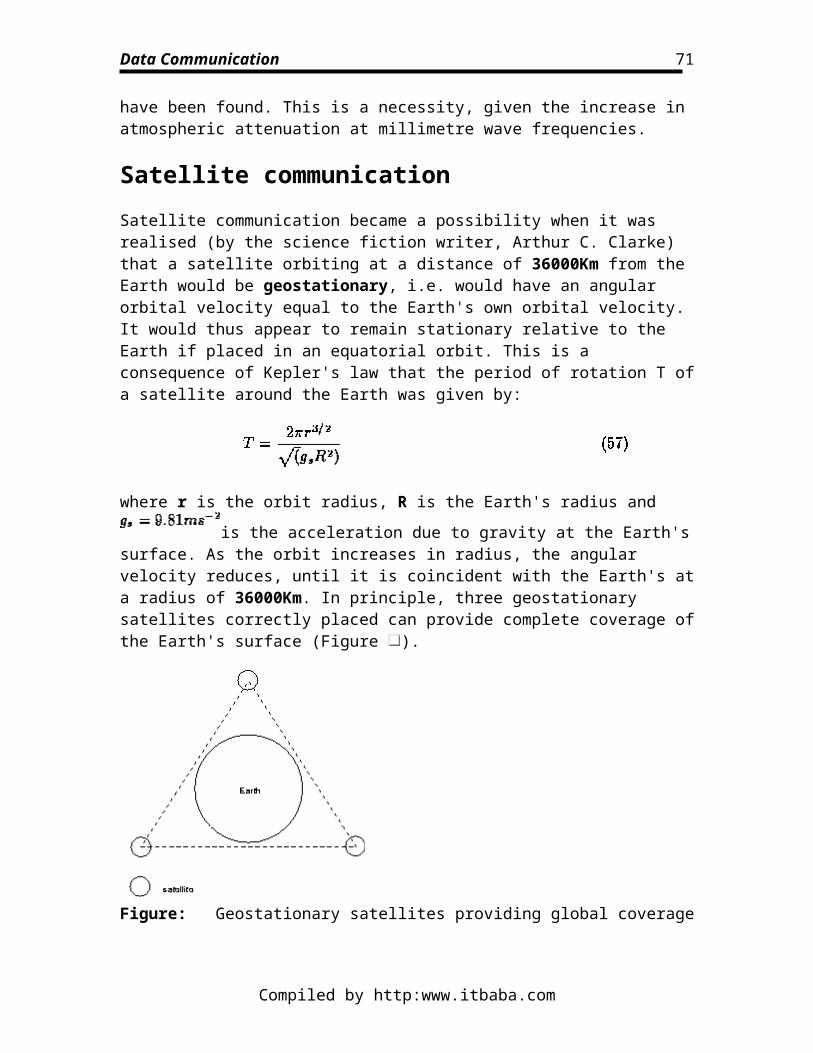
Data Communication

Figure: Example of block sum check showing undetected errors

Parity checking in this way provides good protection against single and multiple bit errors when the probability of the errors are independent. However, in many circumstances, errors occur in groups, or bursts. Parity checking of the kind just described then provides little protection. In these circumstances, a polynomial code is used.

The mechanism of polynomial codes is beyond the scope of this course. We shall content ourselves with a description. Polynomial codes work on each frame. Additional digits are added to the end of each frame. These digits depend on the contents of the frame. The number of added digits depends on the length of the expected error burst. Typically 16 or 32 digits are added. The computed digits are called the frame check sequence (FCS) or cyclic redundancy check (CRC). Before transmission, each frame is divided by a generator polynomial. The remainder of this division is added to the frame. On reception, the division is repeated. Since the remainder has been added, the result should be zero. A non-zero result indicates that an error has occurred.

A polynomial code can detect any error burst of length less than or equal to the length of the generator polynomial. The technique requires the addition of hardware to perform the division. However, with modern integrated circuitry, this hardware is now available inexpensively. CRC error checking is now quite common, and its use will increase.

Error correction codingError correction coding is more sophisticated than error detection coding. Its aim to to detect and locate errors in transmission. Once located, the correction is trivial: the bit is inverted. Error correction coding requires lower rate codes than error detection, often markedly so. It is therefore uncommon in terrestrial communication, where better performance is usually obtained with error detection and retransmission. However, in satellite communications, the propagation delay often means that many frames are transmitted before an instruction to retransmit is received. This can make the task of data handling very complex. Real-time transmission often precludes retransmission. It is necessary to get it right first time. In these special circumstances, the additional bandwidth required for the redundant check-bits is an acceptable price. There are two principle types: Hamming codes and convolutional codes.


71

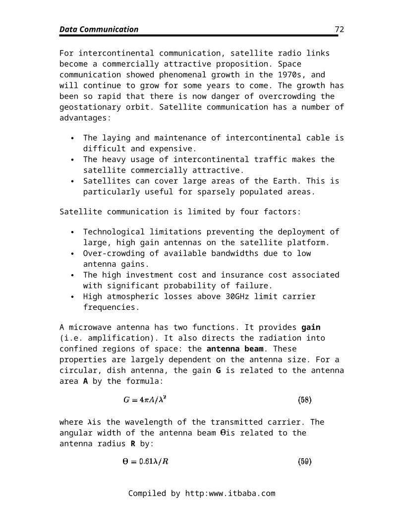
Data Communication

A Hamming code is a block code capable of identifying and correcting any single bit error occurring within the block. It is identified by the numbers K and N; we talk of an

Hamming code. Hamming codes employ modulo 2 arithmetic. Addition in modulo 2 arithmetic is replaced by the exclusive OR (often written XOR or EOR) logic operation. This operation has a truth-table shown in Table .

Table: Truth Table for exclusive OR

The theory of Hamming codes is beyond the scope of our course. An example of a (11, 7) code is given.

Consider a Hamming code to detect and correct for single-bit errors assuming each codeword contains a seven-bit data field, e.g. an ASCII character. for example. Such a coding scheme requires four check bits since, with this scheme, the check bits occupy all bit positions that are powers of 2. Such a code is thus known as an (11, 7) block code

with a rate of 7/11 and a redundancy of . For example, the bit positions of the value 1001101 are:

Bit Position 11 10 9 8 7 6 5 4 3 2 1 Bit value 1 0 0 x 1 1 0 x 1 x x

The four bit positions marked with x are used for the check bits, which are derived as follows. The four-bit binary numbers corresponding to those bit positions having a binary 1 are added together using modulo 2 arithmetic and the four check bits are then the four-bit sum:

11 = 1011 7 = 0111 6 = 0110 3 = 0011 1001

The transmitted codeword is thus:

Bit Position 11 10 9 8 7 6 5 4 3 2 1 Bit value 1 0 0 1 1 1 0 0 1 0 1

Similarly, at the receiver, the four-bit binary numbers corresponding to those bit positions having a binary 1, including the check bits, are again added together and, if no errors have occurred, the modulo 2 sum should be zero:

11 = 1101


72

http://www.cs.ucl.ac.uk/staff/S.Bhatti/D51-notes/node33.html#tblxor

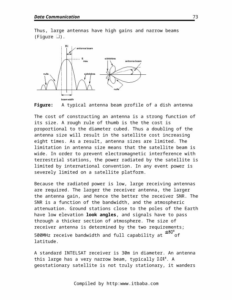
Data Communication

8 = 1100 7 = 0111 6 = 0110 3 = 0011 1 = 0001 0000

Now consider a single-bit error; say bit 11 is corrupted from 1 to 0. The new modulo 2 sum would now be:

8 = 1100 7 = 0111 6 = 0110 3 = 0011 1 = 0001 1011

Firstly, the sum is non-zero, which indicates an error, and secondly the modulo 2 sum, equivalent to decimal 11, indicates that bit 11 is the erroneous bit. The latter would therefore be inverted to obtain the corrected codeword and hence data bits.

Hamming codes suffer from the same difficulty as block-codes. They offer protection against single-bit errors. They offer little protection against burst errors. Convolutional codes are designed to deal with this circumstances. Convolutional codes are different from previous codes we have examined in that they work in a statistical sense. By this we mean that we cannot say that, for example, every single-bit error will be corrected. We can only say that, on average, the use of the convolutional code will improve the error rate. We shall not examine these codes in detail. They are widely used. Their use can typically provide an error rate improvement of 3 orders of magnitude, with a code rate of 1/2.

EncryptionIn all our discussion of coding, we have not mentioned what is popularly supposed to be the purpose of coding: security. We have only considered coding as a mechanism for improving the integrity of the communication system in the presence of noise. The use of coding for security has a different name: encryption. The use of digital computers has made highly secure communication a normal occurrence. It is very much easier to encrypt than it is to decipher. The principle is just that of a combination lock. With a computer, the number of the digits in the lock can be very large. Of course, one still has to keep the combination secure!

The most commonly used encryptions algorithms are block ciphers. This means that the algorithm splits the plaintext (message to be encrypted) into (usually) fixed size blocks which these are subjected to various functions to produce a block of ciphertext. The most common functions are permutations based on expansion and compression and straight "shuffling" transformations. In a straight permutation, the bits of an n bit block are simply reordered. In expansion, as well as being reordered, the group of n bits is


73

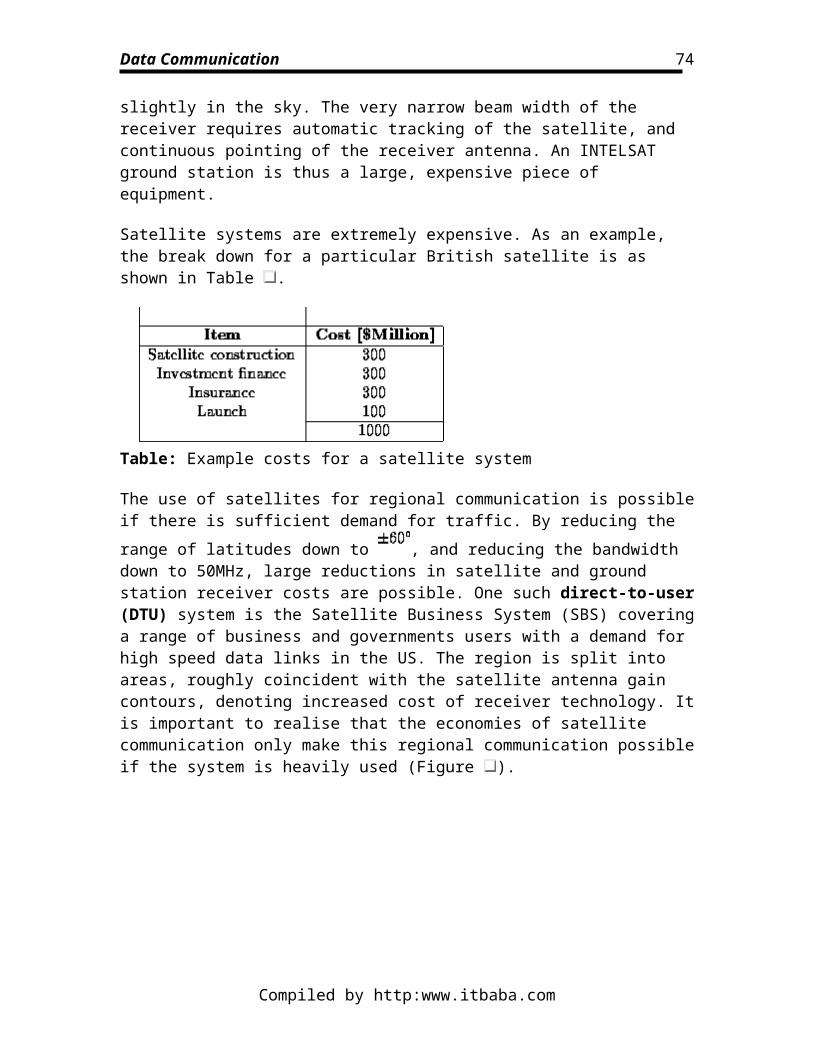
Data Communication

converted to m bits (m > n), with some bits being duplicated. In compression, the n bit block in converted to a p bit block (p < n), with some of the original bits unused (Figure

).

Figure: Examples of block cipher permutations

The most widely used form of encyrption is defined by the National Bureau of Standards and is known as the data encryption standard (DES). The DES is a block cipher, splitting the data stream into 64-bit blocks that are enciphered separately. A (probably) unique key of 56 bits is then used to perform a succession of transposition and

substitution operations. A 56 bit key has possible combinations. Assuming a powerful computer could attempt combinations per second, it would still take over 20 years to break the code. If the code is changed once per year, there is little possibility of it being broken, unless the code breaker has additional information. The DES converts 64 bits of plaintext into 64 bits of ciphertext. The receiver uses the same key to decipher the ciphertext into plaintext.

The difficulty with this method is that each block is independent. This permits an interceptor in possession of the key to introduce additional blocks without the recipient being aware of this fact. In addition, the same plaintext will generate the same ciphertext, a fact of great value to someone attempting to break the code. These disadvantages are removed by chaining. Chaining describes the process of EOR-ing the plaintext of one block with the ciphertext of the previous block. In this way it is not possible to introduce blocks in a transparent fashion, and repetitions of the same plaintext generates different ciphertexts.

Like the combination of a lock, the system is only secure if the key is secure. If the key is changed often, the security of the key becomes a problem, because the transfer of the key between sender and receiver may not be secure. This is avoided by the use of matched keys. In a matched key scheme, the encryption is not reversible with the same key. The message is encrypted using one key, and decrypted with a second, matched key. The receiver makes available the first, public key. This key is used by the sender to encrypt the message. This message is unintelligible to anyone not in possession of the second, private key. In this way the private key need not be transferred. The most famous of such schemes is the Public Key mechanism using the work of Rivest, Shamir and Adleman (RSA). It is based on the use of multiplying extremely large numbers and, with current technology, is computationally very expensive.


74

http://www.cs.ucl.ac.uk/staff/S.Bhatti/D51-notes/node34.html#figpermutations

Data Communication

Broadband ISDNThe original specifications for the intergrated services digital network (ISDN), were based around voice and non-voice telephone-type services: telephony, data, telex, facsimile, as it was hoped that the ISDN would evolve from the (then) emerging digital telephone networks. Indeed, this is one of the reasons that the fundamental element of an ISDN link is the 64Kb/s B-Channel. However, the planning for ISDN was started around 1976, and as technology evolved, so did the requirements of the users that wanted to use this technology. In 1988, the CCITT released a document that described a new set of Broadband ISDN (B-ISDN) services. To distinguish this new concept from the original ISDN service, we now refer to the latter as Narrowband ISDN (N-ISDN).

Since then the CCITT has become the ITU. The B-ISDN work is far from complete, and some of the factors influencing the emergence of the B-ISDN from ITU are:

Demand. Users (both commercial and residential) are showing interest in receiving high speed, reliable services.

Technology. This has been one of the biggest factors. Advances in technology have increased demand, as well as the ability to supply it. As data processing technologies available to the user have become more sophisticated so has his/her demands, while high speed transmission (based on the use of optical fibre), high speed switching and increased processing power make the realisation of these demands possible.

Service integration. There is a need to integrate both circuit switched and packet switched services into one network that can provide interactive and distribution services.

Flexibility. The resulting network must be able to satisfy the needs of the users as well as the network operators in terms of its functionality and usability.

Broadband ISDN services Network architecture Signaling Protocol Reference Model Operation and Maintenance Asynchronous Transfer Mode (ATM) ATM Adaptation Layer Physical Layer; SONET and SDH Connectionless Service

Broadband ISDN services


75










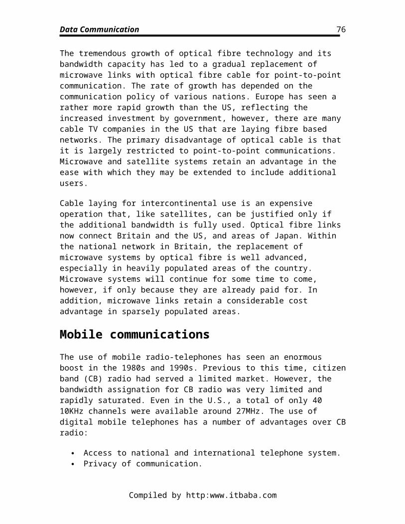
Data Communication

The need for a Broadband ISDN service sprung from the growing needs of the customers. The planned Broadband ISDN services can broadly be categorised as follows:

Interactive services. These are services allowing information flow between two end users of the network, or between the user and the service provider. Such services can be subdivided:

o Conversational services. These are basically end-to-end, real-time communications, between users or between a user and a service provider, e.g. telephone-like services. Indeed, B-ISDN will support N-ISDN type services. (Note also that the user-to-user signaling, user-to-network signaling, and inter-echange signaling are also provided but outside our scope.) Also the additional bandwidth offered will allow such services as video telephony, video conferencing and high volume, high speed data transfer.

o Messaging services. This differs from conversational services in that it is mainly a store-and-forward type of service. Applications could include voice and video mail, as well as multi-media mail and traditional electronic mail.

o Retrieval services. This service provides access to (public) information stores, and information is sent to the user on demand only. This includes things like tele-shopping, videotex services, still and moving pictures, telesoftware and entertainment.

Distribution services. These are mainly broadcast services, are intended for mainly one way interaction from a service provider to a user:

o No user control of presentation. This would be for instance, a TV broadcast, where the user can choose simply either to view or not. It is expected that cable TV companies will become interested in Broadband ISDN as a carrier for the high definition TV (HDTV) services that are forseen for the future.

o User controlled presentation. This would apply to broadcast information that the user can partially control, in that the user can decide which part of it he/she accesses, e.g. teletext and news retrieval services.

However, many of these services have very high throughput requirements, as shown in Table . The burstiness is the ratio of the peak bit rate to average bit rate.

Table: Some Broadband service throughput needs


76

http://www.cs.ucl.ac.uk/staff/S.Bhatti/D51-notes/node36.html#tblbisdnneeds

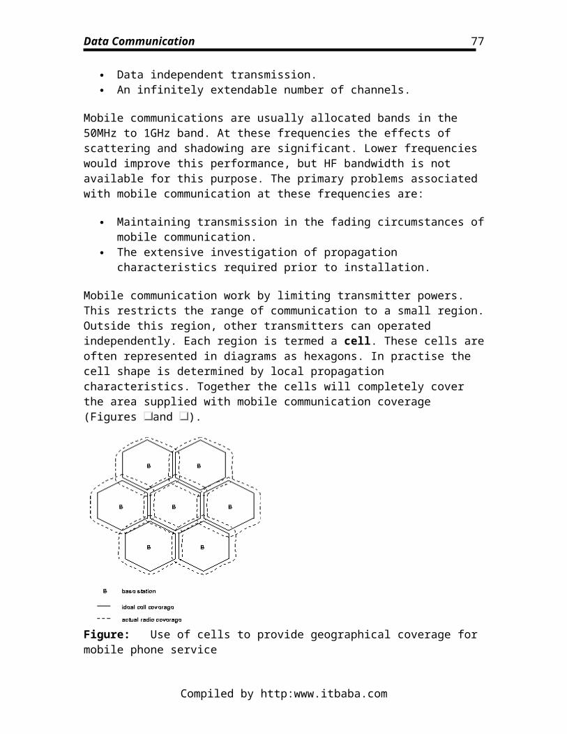
Data Communication

It is clear that high network capacity is required if this kind of service is to be offered to many user simultaneously. The N-ISDN can currently offer interfaces which aggregate B-Channels to give additional throughput, as shown in Table and Table . However, these are not sufficient for our Broadband service requirements.

Table: Narrowband ISDN channels

Table: Narrowband ISDN interfaces

Network architectureThe B-ISDN needs to provide:

Broadband services, as described in the last subsection. Narrowband services (for backwards compatibility). User-to-network signaling, to allow the B-ISDN user to initiate and control

communication. Inter-exchange signaling within the network, to allow the network to provide and

control resources as requested by the B-ISDN user or by another network exchange.

User-to-user signaling, to allow B-ISDN users to send control, operation and maintenance information to each other.

Management facilities for controlling and operating the network.

It is intended that the B-ISDN will offer both connection oriented (CO) and connectionless (CL) services, however, the CO mode of operation is receiving the greatest attention at the moment, while CL service definitions mature. The broadband information transfer is provided by the use of asynchronous transfer mode (ATM), in


77

http://www.cs.ucl.ac.uk/staff/S.Bhatti/D51-notes/node36.html#tblnisdnchannels

http://www.cs.ucl.ac.uk/staff/S.Bhatti/D51-notes/node36.html#tblnisdninterfaces

Data Communication

both cases, using end-to-end logical connections. ATM makes use of small, fixed size (53 octets) cells in which the information is transferred, along the logical connections. Each cell contains a header (5 octets) which is used to identify the logical connection to which the cell belongs.

Each logical connection is accessed as a virtual channel (VC). Many VCs may be used to a single destination and they may be associated by use of a virtual path (VP). There relationship between VCs and VPs with respect to the transmission path is shown in Figure . The transmission path is the logical connection between the two end-points, and consists in reality of many links between network exchanges and switches.

Figure: Transmission path model for Broadband ISDN

The VCs are identified at each end of the connection by a virtual channel identifier (VCI) and user-to-user data VCs are unidirectional. Similarly, the VP is identified by a virtual path identifier (VPI). The VCI/VPI pair uniquely identifies a user-to-user information flow and is carried in each ATM cell header. Both VCIs and VPIs in general have only local significance. The concept of the link can be applied to both VCs and VPs in explaining the use of VCIs and VPIs, and we can say that the VCI/VPI pair identifies a particular link. VCIs and VPIs are used within the network for switching purposes, with virtual channel links and virtual path links being defined as the connection between two points where the either the VC or the VP is switched, respectively, i.e. the link is defined to exist between the two points where the VCI or VPI value is removed or translated (switched). There will be many virtual channel links comprising a virtual channel connection (VCC) and, similarly, many virtual path links in a virtual path connection (VPC). This relationship is shown in Figure .


78

http://www.cs.ucl.ac.uk/staff/S.Bhatti/D51-notes/node37.html#figtxpath

http://www.cs.ucl.ac.uk/staff/S.Bhatti/D51-notes/node37.html#figlayertolayer

Data Communication

Figure: Hierarchical layer to layer relationship in the ATM layer and Physical layer

The transmission path consists of digital sections that are responsible for assembling bit/octet streams. In turn, each digital section may consist of regenerator sections which are sections between two regenerators (repeaters) on a physical link.

The switching of the VCs and VPs is depicted in Figure and Figure .

Figure: Virtual path switch


79

http://www.cs.ucl.ac.uk/staff/S.Bhatti/D51-notes/node37.html#figvpswitch

http://www.cs.ucl.ac.uk/staff/S.Bhatti/D51-notes/node37.html#figvpvcswitch

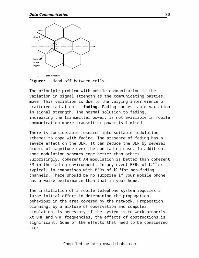
Data Communication

Figure: Virtual path and virtual circuit switch

Figure depicts a scenario which may result in the same VCI being used to identify the VCC at both ends of the transmission path. In this case the VC link may be the same as as the VC connection. However, in general, bpth the VCI and VPI values may be translated in a switch as shown in Figure .

The setting up of VCCs and VPCs between B-ISDN users may be done in a number of ways. For VCCs, one of the following procedures can be used:

A semi-permanent or permanent VCC is established by the network provider as the result of a subscription procedure. This requires no signaling, and the VCCs behave like leased lines.

A switched VCC is established and/or release by the use of user-to-network signaling procedure.

If a VPC already exists between two B-ISDN users, then they may employ user-to-user signaling procedures on one of the the existing VCCs to establish and/or release other VCCs.

A signaling VCC is established by the use of a meta-signaling procedure, using a special meta-signaling VCC.

The cell sequence integrity is guaranteed on any VCC. The QoS for a VCC will have been negotiated at subscription, but may be renegotiated at VCC establishment.

For VPCs, one of the following procedures can be used:

A VPC is established by the network provider as the result of a subscription procedure. This requires no signaling.

A VPC may be established by the B-ISDN user employing network management procedures.


80

http://www.cs.ucl.ac.uk/staff/S.Bhatti/D51-notes/node37.html#figvpswitch

http://www.cs.ucl.ac.uk/staff/S.Bhatti/D51-notes/node37.html#figvpvcswitch

Data Communication

A VPC may be established by the network itself using network management procedures.

Again, cell sequence integrity is guaranteed for each VCC in the VPC but also for the VPC as a whole. This is an improvement over N-ISDN where the use of several B-Channels results in skew in the data sent from one user to another. The QoS required for the VPC can be selected from a set of known classes that have been negotiated with the network provider. Some of the VCIs that could be used for the VPC may be reserved for special purposes, such as operation and management (OAM) activities.

SignalingBroadband ISDN uses out-of-band signaling (as does N-ISDN). Instead of using a D Channel as in N-ISDN, a special VCC can be used for signaling. This also means that the B-ISDN user can have a much more flexible and powerful signaling capability, as further VCCs for signaling can be established as required. As the B-ISDN is meant to backwards compatible with N-ISDN applications, the B-ISDN also provide N-ISDN signaling. Also, the B-ISDN services bring their own requirements for more powerful signaling:

Establish, release and maintain VCCs as required. Negotiate and/or renegotiate the QoS for VCCs. Allow mutli-connection calls, i.e. composite calls that require several different

types of information flow to the same destination. For instance, a multimedia call that carries voice, video and data may use one VC each for the voice, video and data, each with its own QoS requirements and synchronisation requirements.

Allow multi-party calls, i.e. calls between more than two end-points. For instance a conference call. This type of call requires facilities to allow users to leave or join the call/conference. If the call is a multi-media conference, then the multi-connection signaling facility will also be required and should operate in harmony.

B-ISDN uses dedicated signaling virtual channels (SVCs). There are four types as shown in Table .

Table: SVCs at the B-ISDN user-to-network interface

There is only meta-signaling channel per interface and it is permanent. It is used to set up instances of the point-to-point SVC as required. It is identified by the use of a specially allocated VCI/VPI.


81

http://www.cs.ucl.ac.uk/staff/S.Bhatti/D51-notes/node38.html#tblsvc

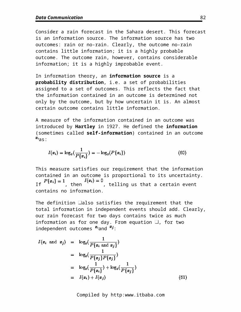
Data Communication

The broadcast SVCs are directed from network to user. The general broadcast SVC is permanent and provides signaling information to all network users. The selective broadcast SVC is optionally set up by the network provider to provide additional signaling services to only certain terminals.

The point-to-point SVC exists only while it is active and is used to establish, maintain, control and release data VCCs between to end points.

Protocol Reference ModelThe network is described in terms of a protocol reference model (PRM) (Figure ). Not all of the PRM is fully defined. The main aspects of the model are that it can be viewed in terms of the three planes -- user plane, control plane and management plane -- and in terms of the 3 layers -- ATM adaptation layer, ATM layer and the Physical layer.

Figure: Broadband ISDN protocol reference model

The functions of the layers are as follows:

ATM adaptation layer (AAL). This layer is responsible for mapping the service offered by ATM to the service expected by the higher layers. It has two sublayers.

o Convergence sublayer (CS). Responsible for presenting the ATM service to the higher layers. The functionality of this sublayer is very much dependent on the higher layer service.

o Segmentation and reassembly (SAR). This layer is responsible for, at the transmitter, splitting the higher level PDU into 48 octet chunks, and at the receiving side, to reassemble the 48 octet chunks back into the original PDU.

ATM Layer. This layer is independent of the physical medium over which transmission is to take place. It has four functions:


82

http://www.cs.ucl.ac.uk/staff/S.Bhatti/D51-notes/node39.html#figbisdnprm

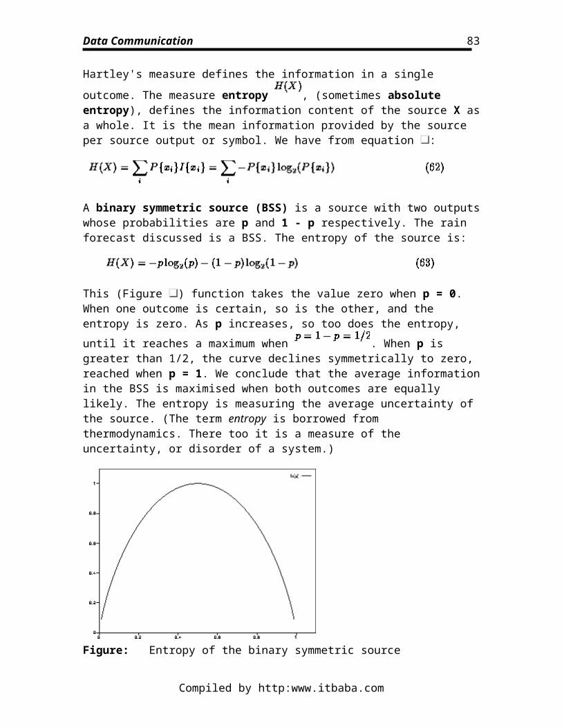
Data Communication

o Generic flow control (GFC) function. This can be used to alleviate short term overload conditions above the ATM layer, as it is accessible by the user.

o Cell header generation and extraction. At the transmitter, adds header information to a cell, and at the receiver removes it.

o Cell multiplex and demultiplex. At the transmitter, multiplex cells into one continuous stream, and at the header demultiplex the cells according to VPI and VCI values.

Physical layer. This consists of two sublayers: o Transport Convergence (TC). This sublayer has five functions:

Cell rate decoupling. Insertion and extraction of idle cells. Header error control (HEC) generation and verification. In the

transmitter, generation of the HEC, and in the receiver checking of the HEC. The HEC that is used can detect and correct a 1 bit error and can further detect certain multiple bit errors.

Cell delineation. In the receiver, detection of cell boundaries. Transmission frame adaptation. Adapts cell flow according to

the payload of the Physical level frame being used, e.g. for SDH. Transmission frame generation and recovery. At the

transmitter, generates Physical level frames, and at the receiver, extracts the ATM cells from the Physical level frame.

o Physical medium (PM). This contains two sublayers: Bit timing. Insertion and extraction of bit timing information and

generation and reception of waveforms. Physical medium. Bit transmission, bit alignment and optical

electrical conversion, if required. (The physical medium need not be optical, at least for transmission rates of 155Mb/s and lower.)

This (sub-)layering of the PRM is depicted in Figure .


83

http://www.cs.ucl.ac.uk/staff/S.Bhatti/D51-notes/node39.html#figbisdnlayerfunc

Data Communication

Figure: Broadband ISDN layer functionality

The management plane consists of two functions to perform layer management and plane management. The plane management is not layered as the other layers are. This is because it relies needs information on all aspects of the the system to provide management facilities for the systems as a whole. The layer management provides information and control facilities for the protocol entities that exists in each individual layer. This includes operation and maintenance (OAM) functions for each layer.

The control plane is responsible for the supervision of connections, including call set-up, call release and maintenance.

The user plane provides for the transfer of user information. It also includes mechanisms to perform error recovery, flow control etc.

Broadband ISDN intends to offer many Mb/s to the user, but intends to remaim backwards compatible with Narrowband ISDN. Indeed, the Narrowband services will eventually need to be offered over the global Broadband network to come. To this extent the user interface to Broadband ISDN is very similar to that for Narrowband ISDN. Figure shows the position of the user to network interface (UNI), as well as the internal network to network interface (NNI) for Broadband-ISDN. We will concentrate our attention mainly on the UNI. The UNI is accessed at the reference point or (Figure ).


84

http://www.cs.ucl.ac.uk/staff/S.Bhatti/D51-notes/node39.html#figbisdninterface

http://www.cs.ucl.ac.uk/staff/S.Bhatti/D51-notes/node39.html#figbisdnuniconfig

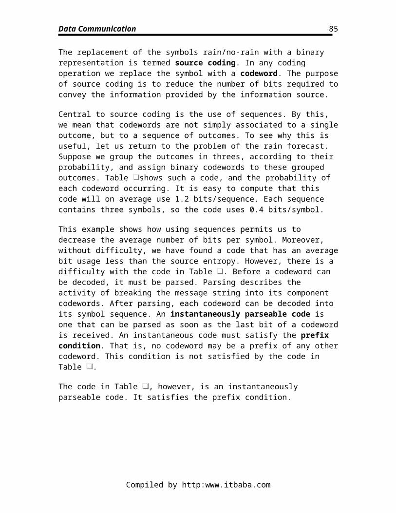
Data Communication

Figure: Broadband ISDN user and network interfaces

Figure: Broadband ISDN UNI configuration reference points

Note that in Figure , it is expected that Narrowband ISDN (or even other PSTN) equipment will be able to connect to the Broadband network via a suitable terminal adaptor. The various functional groups are now described:

B-NT1. This group contains functions that are considered to be part of OSI layer 1. It represents the physical connection point to the network, i.e. the socket on the wall. It includes functions such as:

o Line transmission termination. Provision of the physical connection. o Transmission interface handling. The interface to the transmission

channel, be it electrical or optical. o Operation and Maintenance (OAM). This is not normally associated

with the socket in the wall. However, it is expected that for B-ISDN, more sophisticated management capabilities will be required than at present.

B-NT2. This group contains OSI layer 1 and higher OSI layer functions: o Adaptation functions. For different physical media and network

topologies. o Multiplexing and demultiplexing. The user data may be sent and

received on several VCCs and VPCs. o Buffering. User data may be sent and/or received at varying rates with

respect to the B-ISDN user and the network.


85

http://www.cs.ucl.ac.uk/staff/S.Bhatti/D51-notes/node39.html#figbisdnuniconfig

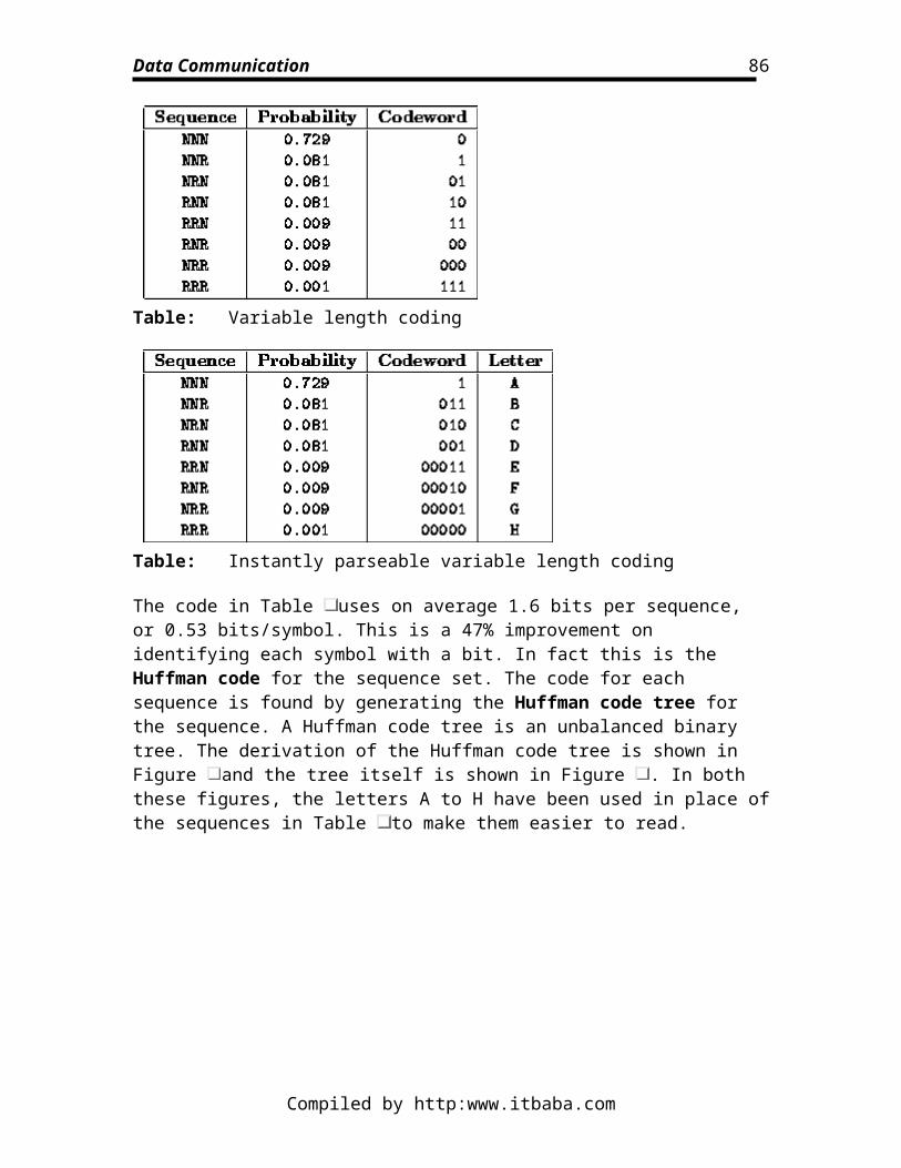
Data Communication

o Signaling. VCCs/VPCs must be established, controlled and released. o Interface. Interaction with the B-ISDN user.

B-TE1. Equipment requiring B-ISDN access. B-TA. Equipment allowing connection of other B-ISDN, N-ISDN and non-ISDN

equipment. B-TE2. B-ISDN with special interface needs or N-ISDN equipment. TE2. Non-ISDN equipment.

Note that these are logical units. The physical implementation may be quite different. For instance, it may be common to find the following in the same physical unit, depending on need: B-NT1 and B-NT2; B-TE1 and B-NT2; B-TA and B-TE2 etc.

Further, the way in which the terminal equipment is connected to the user-to-network interface via B-NT1/B-NT2 is not restricted with respect to local topologies (Figure ).

Figure: Broadband ISDN multiple interface configurations


86

http://www.cs.ucl.ac.uk/staff/S.Bhatti/D51-notes/node39.html#figbisdnifconfigs

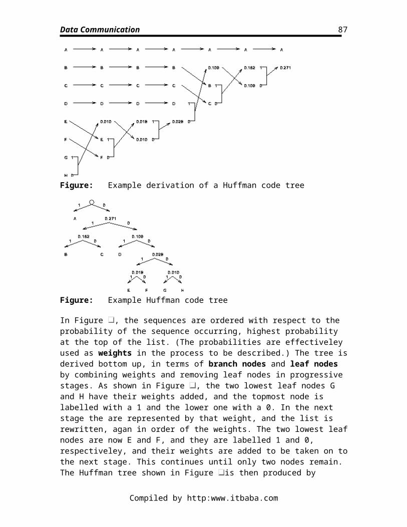
Data Communication

The B-NT2 equipment is considered to be the customer premisis equipment (CPN) (Figure ). This could in real terms be an private branch exchange (PBX) or other local switch.

Figure: B-ISDN customer premisis network configuration

The discussion above has mentioned the OSI reference model. This was developed in collaboration between the ISO and the (then) CCITT. It seems surprising therefore that there is no defined relationship between the B-ISDN PRM and the OSI reference model. Figure is the author's view of the relationship between the two.

Figure: Broadband ISDN PRM compared with OSI model

As there is unlikely to be a user interface directly to the AAL, included in this figure are the interfaces to the service classes defined by the ATM Forum for the UNI:

Constant bit rate (CBR). The CBR service offers a very simple, reliable guaranteed channel that effectively acts as a circuit emulation. The QoS of this service must be maintained throughout the lifetime of a CBR connection, as the data rate is expected to be constant. It is intended for use by applications with stringent real-time constraints on delay and jitter, e.g.\ real-time video.

Variable bit rate (VBR). This service is also intended for use by by real-time applications. However, it differs from CBR in that it does not expect the data rate to be constant, i.e. the sources may use variable bit rate coding for efficiency and also be statistically multiplexed.


87

http://www.cs.ucl.ac.uk/staff/S.Bhatti/D51-notes/node39.html#figbisdncpn

http://www.cs.ucl.ac.uk/staff/S.Bhatti/D51-notes/node39.html#figbisdnosi

Data Communication

Available bit rate (ABR). This service class offers the B-ISDN user some degree of fairness, and also control of loss or delay with respect to QoS, but is intended for non real-time applications. It is likely that ABR QoS statements will specify that there are minimum acceptable parameters, but that if better QoS should become available then it will be used. ABR is intended for use by unit-oriented applications such as database access and electronic mail.

Unspecified bit rate (UBR). UBR is intended for applications that send data very sporadically and the use of CBR, VBR or ABR would be wasteful of resources. In fact, this service class is effectively a best-effort approach which is similar to today's IP. Applications that use this service would have non-real time requirements and not be too sensitive to loss, e.g. file transfers.

Operation and MaintenanceThe operation and maintenance (OAM) of the B-ISDN network has five main actions:

Performance monitoring. Managed entities are continuously or periodically monitored in order to generate maintenance event information.

Defect and failure detection. Errors or malfunctions in the managed entities are detected or predicted resulting in the generation of maintenance event information or service alarms.

System protection. To offer some degree of fault tolerance, the effect of failures in managed entities are minimised by the use of backups, standbys or other resources, and the failed entity is excluded form the normal operation of the system.

Failure or performance information. Communication of failure and performance information as alarms to other managed entities in the management plane. Also acts as a response service to status report requests.

Fault localisation. Use of test systems, both internal and external, to determine whether information about faults is complete or sufficient for other actions to take place.

These actions are supported by the use of OAM information flows in the ATM layer and Physical layer (Figure ).


88

http://www.cs.ucl.ac.uk/staff/S.Bhatti/D51-notes/node40.html#figlayertolayeroam

Data Communication

Figure: OAM information flows in ATM layer and Physical layer

Other management capabilities such as use of the TMN (Telecommunications Management Network) may also be employed in conjunction with (or instead of!) the OAM.

Asynchronous Transfer Mode (ATM)To provide the new B-ISDN services, use of a technology called asynchronous transfer mode (ATM) is specified by ITU. ATM is a connection-oriented technique based on the use of fixed size packets termed cells. These cells are 53 octets in size, with 5 octets used for the cell header, and the remaining 48 octets for data (Figure ).

Figure: An ATM cell

The term asynchronous transfer mode needs some explanation. The words transfer mode say that this technology is specific way of transmitting and switching through the network. The term asynchronous refers to the fact that the packets are transmitted using asynchronous techniques, and the two end-points need not have synchronised clocks. Also, the use and allocation of cells and their subsequent multiplexing and transmission through the network is determined in an asynchronous fashion, e.g. on demand, and is


89

http://www.cs.ucl.ac.uk/staff/S.Bhatti/D51-notes/node41.html#figatmcell

Data Communication

independent of the user (Figure and Figure ). ATM will support both circuit switched and packet switched (sometimes referred to as circuit mode and packet mode, respectively) services.

Figure: The principle of synchronous transfer mode

Figure: The principle of asynchronous transfer mode

There is much to know about ATM, however, here we will consider only the transmission aspects, by looking at the Physical layer and the ATM layer.

There are several types of cells to consider, some are passed all the way through to the ATM layer, while others never proceed beyond the Physical layer:

Assigned Cell. (ATM Layer) A cell which is used to provide the service to the higher layers. This is the cell type that is used in transporting the higher level PDU.

Unassigned cell. (ATM Layer) An ATM layer cell which is not an assigned cell. Valid cell. (Physical layer) Any cell that does not contain header errors, either

through successful transmission or after being corrected by the physical layer. Invalid cell. (Physical layer) A cell with an error in its header that can not be

corrected. It will be discarded by the physical layer. Idle cell. (Physical layer) A cell that is inserted/extracted by the physical layer for

the purposes of payload capacity adaptation.

As explained earlier, there are two interfaces to the B-ISDN to consider -- the user-to-network interface (UNI) and the network-to-network interface (NNI). For these two interfaces the internal structure of the ATM cell header is slightly different, as shown in Figure and Figure .

The various parts of the cell header are:


90

http://www.cs.ucl.ac.uk/staff/S.Bhatti/D51-notes/node41.html#figstmprinciple

http://www.cs.ucl.ac.uk/staff/S.Bhatti/D51-notes/node41.html#figatmprinciple

http://www.cs.ucl.ac.uk/staff/S.Bhatti/D51-notes/node41.html#figatmuniheader

http://www.cs.ucl.ac.uk/staff/S.Bhatti/D51-notes/node41.html#figatmnniheader

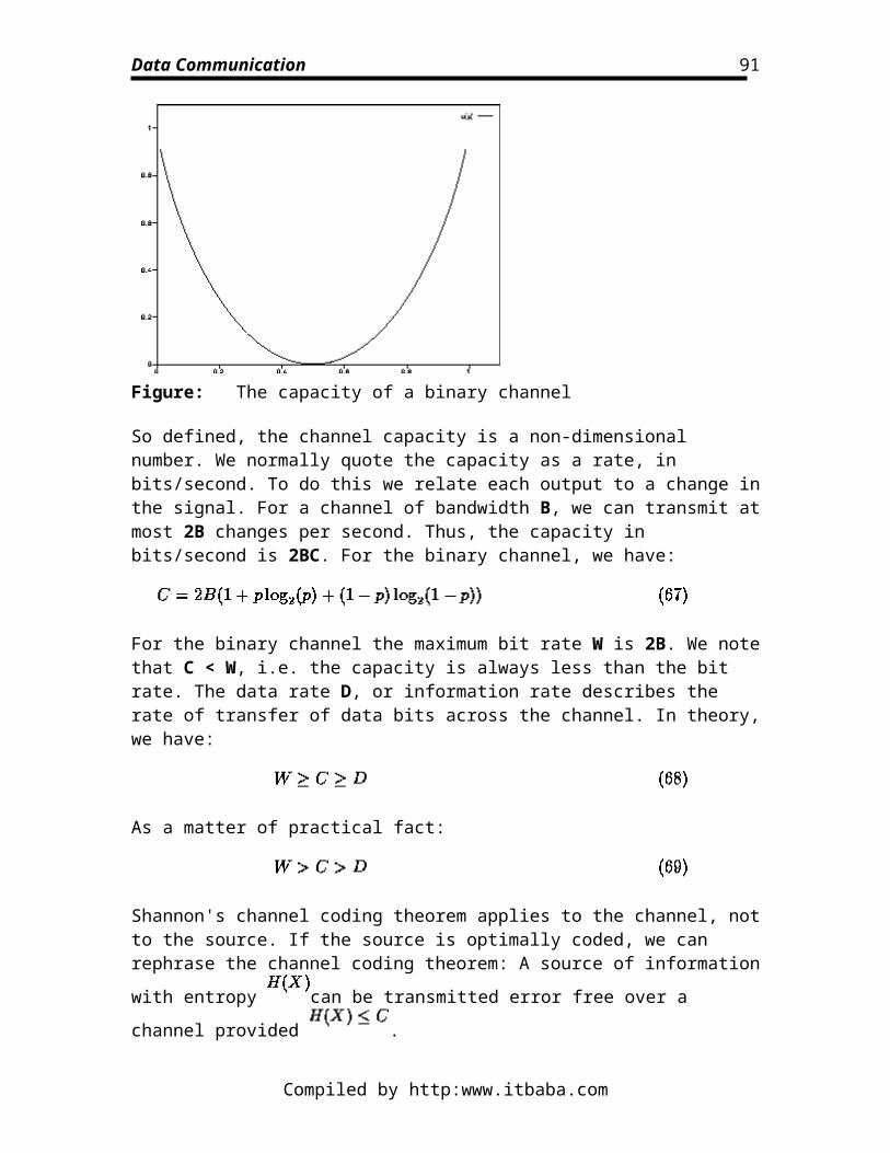
Data Communication

Generic flow control (GFC). (4 bits) Default value 0000. The exact use of this field is, as yet, not fully defined. This is used only in assigned or unassigned (i.e. ATM layer cells).

Virtual path identifier (VPI). (8 or 12 bits) This is used for physical layer routing, together with the;

Virtual circuit identifier (VCI). (16 bits) This is used in conjunction with the VPI field to provide physical level routing. Many cells with different VCIs may have the same VPI. Some VCI/VPI values are pre-assigned for special purposes (Table ).

Payload type (PT). (3 bits) Some PT values -- PT identifiers (PTIs) -- are pre-assigned (Table ) for special purposes.

Cell loss priority (CLP). (1 bit) Flag stating whether or not this cell can be dropped in the prescence of network congestion or other network difficulties. A value of 0 means that this cell has high priority and should not be discarded.

Header error control (HEC). (8 bits) This is used by the physical layer for detecting and correcting errors in the cell header.

Figure: ATM cell header for UNI

Figure: ATM cell header for NNI


91

http://www.cs.ucl.ac.uk/staff/S.Bhatti/D51-notes/node41.html#tblvci

http://www.cs.ucl.ac.uk/staff/S.Bhatti/D51-notes/node41.html#tblpti

Data Communication

Table: Pre-assigned VCI/VPI values for ATM cells

Table: Pre-assigned PTI values for ATM cells

ATM Adaptation LayerThe purpose of the ATM Adaptation Layer (AAL) is to adapt the PDUs passed down from the higher layer onto ATM cells. As the higher level PDUs may in general be of an arbitrary size, so one of the two sublayers in the AAL is responsible for segmentation and reassembly (SAR) of the higher layer PDUs. The other sublayer, the convergence sublayer (CS), is responsible for packaging the higher layer PDU with any additional information required for the adaptation necessary and offering an interface to the B-ISDN user. As mentioned previously, there are many and varied requirements for applications using the B-ISDN and as there are several AAL protocols defined. The classification of these protocols was guided by considering the following parameters:

Timing relationship. The (non-)requirement for synchronisation between the receiver and sender.

Bit rate. Constant or variable. Connection mode. Connection oriented or connectionless.


92

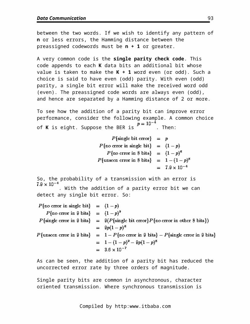
Data Communication

A summary of the (sensible) combinations of these parameters is given in Figure . Each of these classes may be looseley associated with the the ATM Forum classes described previously: Class A, CBR; Class B, VBR; Class C, ABR(ish); Class D, UBR. This mapping also give example use of the various classes. The various AAL classes are provided by several AAL protocols identified by a type number. The use of a particular AAL type for the provision of a particular service is not wholy well defined.

Figure: AAL service classification

AAL Type 0. This is effectively a NULL AAL. It is not really an official AAL type but is mentioned for completeness.

AAL Type 1. This AAL type is normally used by Class A (CBR) services. The function performed by this AAL are:

Segmentation and reassembly of user information. Handling of cell delay variation (jitter). Handling of cell reassembly variation. Handling of lost and misinserted cells. Source clock frequency recovery at receiver. Source data structure recovery at receiver. Monitoring and handling of AAL-PCI bit errors. Monitoring and (possibly) correcting the bit errors in the user information field. For circuit emulation, monitoring and maintenance of end-to-end QoS.

AAL Type 2. This AAL type would be used with Class B (VBR). This type is not well defined and it seems possible that the it may be merged with AAL Type 1 in the future. Some of its functions are similar to ALL Type 1:

Segmentation and reassembly of user information. Handling of cell delay variation (jitter). Handling of lost and misinserted cells. Source clock frequency recovery at receiver. Monitoring and handling of AAL-PCI bit errors. Monitoring and (possibly) correcting the bit errors in the user information field.

It also has the additional functions:

Handle SDUs from a variable bit rate source. Transfer timing information between source and destination. Notify the higher layers of uncorrectable errors in AAL.


93

http://www.cs.ucl.ac.uk/staff/S.Bhatti/D51-notes/node42.html#figaalserviceclasses

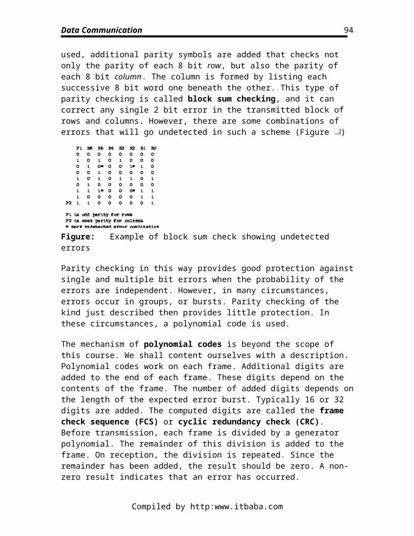
Data Communication

AAL Type 3/4. There was once separate Type 3 and Type 4 AALs, but they have now been merged. This AAL is now intended to support both Class C (ABR) and Class D (UBR) services.

In this AAL, the convergence sublayer is split into two (Figure ), the service specific convergence subslayer (SSCS) and the common part convergence sublayer (CPCS). The SSCS is application dependent, i.e. it could be for a VBR video application. The CPCS is responsible for constructing PDUs that can be sent to the other end user. There are two modes of operation of ALL Type 3/4; message mode and streaming mode.

Figure: AAL Type 3/4 sub-layering

The message mode is intended for use framed data where the AAL-SDU is a logical unit of data with respect to the B-ISDN user (Figure ). It allows the the transport of a single AAL-SDU in one or (optionally) more than one CS-PDU. The CS-PDU may be then further spilt into several SAR-PDUs. The AAL-SDU can be of an arbitrary size.

Figure: AAL Type 3/4 message mode service


94

http://www.cs.ucl.ac.uk/staff/S.Bhatti/D51-notes/node42.html#figaal34

http://www.cs.ucl.ac.uk/staff/S.Bhatti/D51-notes/node42.html#figaal34messagemode

Data Communication

In streaming mode, the AAL-SDUs are of fixed size and one or more of them may be transported in a single CS-PDU (Figure ). Each AAL-SDU is delivered in a separate SAR-PDU.

Figure: AAL Type 3/4 streaming mode service

In both cases, the SAR sublayer provides error detection and both these modes can offer the following operational procedures:

Assured operation. Flow control and retransmission of missing or erroneous AAL-SDUs. Flow control restricted to point-to-point connections at the ATM layer and point-to-multipoint flow control possible.

Non-assured operation. No retransmission of missing or erroneous SAR-PDUs. Optionally deliver erroneous PDUs to user. Allow flow control for point-to-point connections but not point-to-multipoint.

This AAL type also provides multiplexing at the SAR sublayer.

AAL Type 5.

This AAL type provides similar services as AAL Type 3/4, but has a reduced overhead when compared to AAL Type 3/4. It is intended for use by VBR sources with timing relationship between source and destination. It has identical modes and operational procedures as AAL Type 3/4. The difference is that this AAL does not provide the AAL Type 3/4 multiplexing capability. The SAR sublayer accepts only AAL-SDUs that are an integer multiple of 48 octets. So, it would be possible for this AAL to offer an efficient cell based interface to the B-ISDN user.

AAL Types 1 and Type 2 are not used much.

AAL Type 3/4 has been chosen for the provision of the Bellcore switched multi-megabit data service (SMDS), the European version of which is the connectionless broadband data service (CBDS).

AAL Type 5 has been selected by the IETF to provide IP services over ATM.


95

http://www.cs.ucl.ac.uk/staff/S.Bhatti/D51-notes/node42.html#figaal34streamingmode

Data Communication

Physical Layer; SONET and SDHFor B-ISDN, two transmission rates are currently specified; 155Mb/s and 622Mb/s, although it is highly likely that other higher rates will be standardised (Table ).

Table: SONET and SDH data rates and payload rates

To achieve these rates, the physical layer uses a structuring called synchronous digital hierarchy (SDH). This is a ITU standard based heavily on earlier work by ANSI called synchronous optical network (SONET). For our interests the two are practically identical, and so further, only reference to SDH will be made, with specific differences in SONET being highlighted where necessary. SDH specifies a hierarchy of signals that are multiples of 155.52Mb/s to achieve higher data rates. For instance, the 155Mb/s rate, SDH uses a 9 270 octet frame. This frame is repeated with a frequency of 8KHz, so achieving a rate of 155Mb/s (Figure ). The frame consists of 81 octets of section overhead (SOH) and the rest of the frame, which we will call the payload, is filled with ATM cells. The capacity available to the network user is then the payload rate. The path overhead (POH) are special control octets. The AU-4 pointer give the location of the VC-4 container which holds the ATM cells. There may not be an integral number of cells in the VC-4.

The 622Mb/s rate can be achieved simply extending the 155Mb/s SDH frame by increasing the field sizes (Figure ).


96

http://www.cs.ucl.ac.uk/staff/S.Bhatti/D51-notes/node43.html#tblsdh

http://www.cs.ucl.ac.uk/staff/S.Bhatti/D51-notes/node43.html#figstm1

http://www.cs.ucl.ac.uk/staff/S.Bhatti/D51-notes/node43.html#figstm4

Data Communication

Figure: Frame structure for 155.520Mb/s SDH-based interface

Figure: Frame structure for 622.080Mb/s SDH-based interface

Some of the Physical layer specifications for the optical transmission of the signal are given in Table .


97

http://www.cs.ucl.ac.uk/staff/S.Bhatti/D51-notes/node43.html#tblsdhoptical

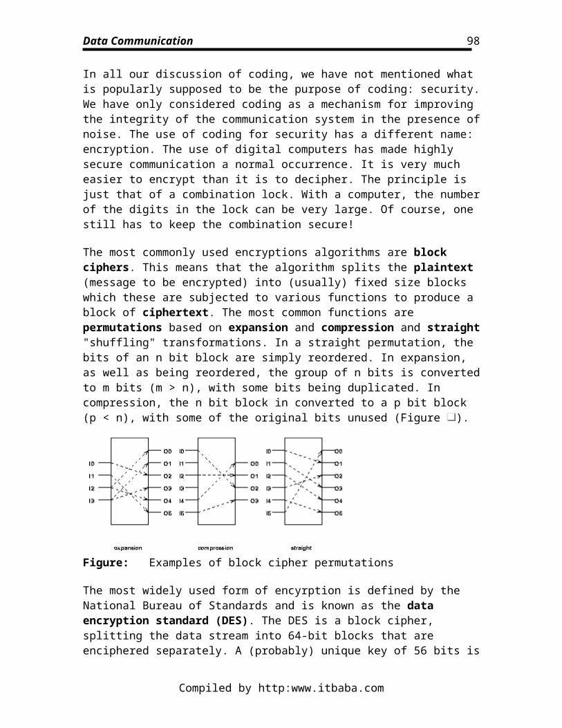
Data Communication

Table: Optical interface characteristics for SDH

Connectionless ServiceB-ISDN can also provide a connectionless (CL) service. This type of service is likely to be important as one of the first uses of B-ISDN is likely to be LAN/MAN interconnection. Most LANs and MANs use CL services and protocols at the subnetwork level, e.g. Ethernet.

There is always the possibility of indirect provision of CL services by putting the CL service functions (CLSF) outside the B-ISDN network and using ATM connections, i.e. a form of simulated CL (Figure ). The CLSF would use ATM connections to the required destinations. These connections could be (semi-)permanent VCCs, pre-configured services specially supplied by the network provider or switched connections set up on demand. In the latter case, the user-to-network signaling would need to be very fast and efficient and the VCC set-up time would have to be minimised in order that the characteristics of the CL service expected by the B-ISDN user are maintained. Use of the permanent or reserved VCCs is obviously wasteful of resources.

Figure: Indirect provision of connectionless service on B-ISDN

A connectionless service can also be provided by the B-ISDN directly. Connectionless service functions (CLSFs) would be enabled either by a specialised connectionless service provider or by the B-ISDN itself. The CL service would use special connections between the user and the CLSF, which could be permanent, semi-permanent or switched circuits. Semi-permanent connections could be either VPCs with several VCCs offering


98

http://www.cs.ucl.ac.uk/staff/S.Bhatti/D51-notes/node44.html#figindirectclsf

Data Communication

CL services, or a single VCC. With switched connections would only allow the use of a single VCC at a time. In the case of a switched connection service, if the connection can not be established when the data transfer is requested, the data will be rejected by the CLSF.

Figure: Direct provision of connectionless service on B-ISDN

SwitchingSwitching is concerned with connecting any communicating end-points in a network with out the need of having direct, dedicated connections between all the possible end-points in the network. It's purpose is to efficiently determine the transmission links that are used in transporting information between two end-points. It is essentially a Physical Layer (Layer 1) and Data-Link Layer (Layer 2) function, and although its description will involve some description of routing type problems, it should not be confused with Network level (Layer 3) routing functions.

Transfer Modes Switches Switching services in networks

Transfer Modes


99




Data Communication

The type of switching used can be heavily dependent on the type of subnetwork, specifically if the subnetwork is connection of a connection oriented (CO) or a connection less (CL) nature. This can be described by its transfer mode, the way in which information is passed along the transmission path, multiplexed as well as switched.

Circuit Switching (CS). This is used in traditional telephone networks and also in N-ISDN. This involves the two end-points first setting up a (logical) connection between them ( connection establishment phase). Then, their follows the required information exchange ( data transfer phase), after which the connection is dropped ( connection release phase). Any network resources that are required for the connection must be made available at connection establishment, maintained during data transfer and then freed at connection release. This kind of technology uses time domain multiplexing and synchronous transfer mode to allocate available capacity to users.

Multi-rate circuit switching (MRCS). CS is inflexible and can be wasteful of resources. Although similar to CS, MRCS allows different basic rates by defining different channel types, and a user can choose which channel type to use. For instance, in with N-ISDN, H0, H11 etc aggregate channels can be used when required. The basic channel rate must be carefully chose in a trade-off between flexibility and efficiency. This type of transfer mode has a limited number of channels of each type that can be used, so is not very future-proof. For example, it may only be possible to offer a given number of H0 channels at a single exchange.

Fast circuit switching (FCS). Both CS and MRCS are inefficient for bursty data. FCS attempts to overcome this problem by caching some information about the type of connection and resources required, but does not actually set up the connection. When data transfer is requested, the cached information is used to set up a connection, and then the connection is torn down again after data transfer. Because there is no resource reservation, as with CS or MRCS, the Quaility of Service (QoS) may not always be guaranteed. There are also descriptions of mechanisms combining MRCS and FCS, but they become complex to design and implement, and one of the biggest problems is how to handle the high signaling rate involved.

Asynchronous transfer mode (ATM). This uses a CO based approach, setting up a connection, and multiplexing and switching fixed size cells onto the the connection. The connection has reduced functionality from the traditional CS type connection and is made possible by making assumptions about the reliability and capacity of the subnetwork. The fixed size cells and the asynchronous allocation of available network capacity means that this transfer mode is flexible and future-proof.

Frame switching. This is similar to frame relay, differing only in the way it allows error control at the data-link level. Frame relay has no end-to-end error control or flow control, while frame switching has both of these.

Frame relay. This is similar to (and precursor to) ATM. Again, it is CS with reduced functionality, however the frames do not have to be of a fixed size.


100

Data Communication

Packet switching (PS). In PS there is no prearranged connection between the end-points, and the information flow between them is contained in packets, each with its own header giving relevant information to facilitate switching, error control, flow control etc.

ATM, frame relay and frame switching seem very similar. Indeed, sometimes frame relay and ATM are considered synonymous, however we will make the distinction as there are two different sets of CCITT recommendations describing each.

Table: The functions of some transfer modes

This spectrum of transfer modes is summarised in Figure and Table gives a short summary of the main functional differences between the some of the transfer modes mentioned above, and the following Notes are referred to:

Note 1: As fixed-size cells and fixed cell formats are used in ATM and SDH, there is no need for bit stuffing.

Notes 2: Some AALs may provide error checking for the data portions of the AAL-SDU, however this is not part of the ATM or B-ISDN physical layer.

Note 3: The assignments of VCI/VPI values that are used for multiplexing are for left to the AAL ro B-ISDN user.

Figure: The range of transfer modes


101

http://www.cs.ucl.ac.uk/staff/S.Bhatti/D51-notes/node46.html#figtransfermodes

http://www.cs.ucl.ac.uk/staff/S.Bhatti/D51-notes/node46.html#tbltransfermodefunctions

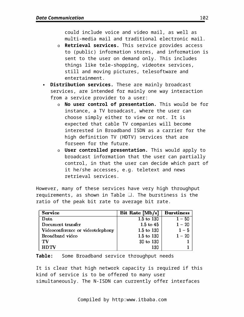
Data Communication

SwitchesThe purpose of switching is to provide interconnection between all the nodes on a network without the need for single connections between each pair of nodes (Figure ).

Figure: Direct connection between nodes is in efficient

We require switching technology that provides a mechanism to establish connectivity as and when required. As we saw in the last subsection, the nature of the switching required depends on the transfer mode. In this subsection, we discuss something of the physical nature of the switches themselves. Before we go on to describe the types of switches, it is worth defining some terminology:

Switching element: This is a basic building block of a switch. A switching element will consist of a input controllers and output controllers which provide the input and outputs, respectively, to an interconnection network (Figure ).

Switching fabric: This is an interconnection of switching elements to facilitate a particular switching mechanism. The switching fabric is characterised by the types and interconnection of its switching elements.

Switching elements have have many forms, however they have the following two common problems that must be resolved:

Collisions: This occurs when more than one inputs are destined for the same output.

Blocking: This occurs when the progress of one message through the interconnection network is stopped by a message that is not destined for the same output.


102

http://www.cs.ucl.ac.uk/staff/S.Bhatti/D51-notes/node47.html#fignoswitch

http://www.cs.ucl.ac.uk/staff/S.Bhatti/D51-notes/node47.html#figswitchingelement

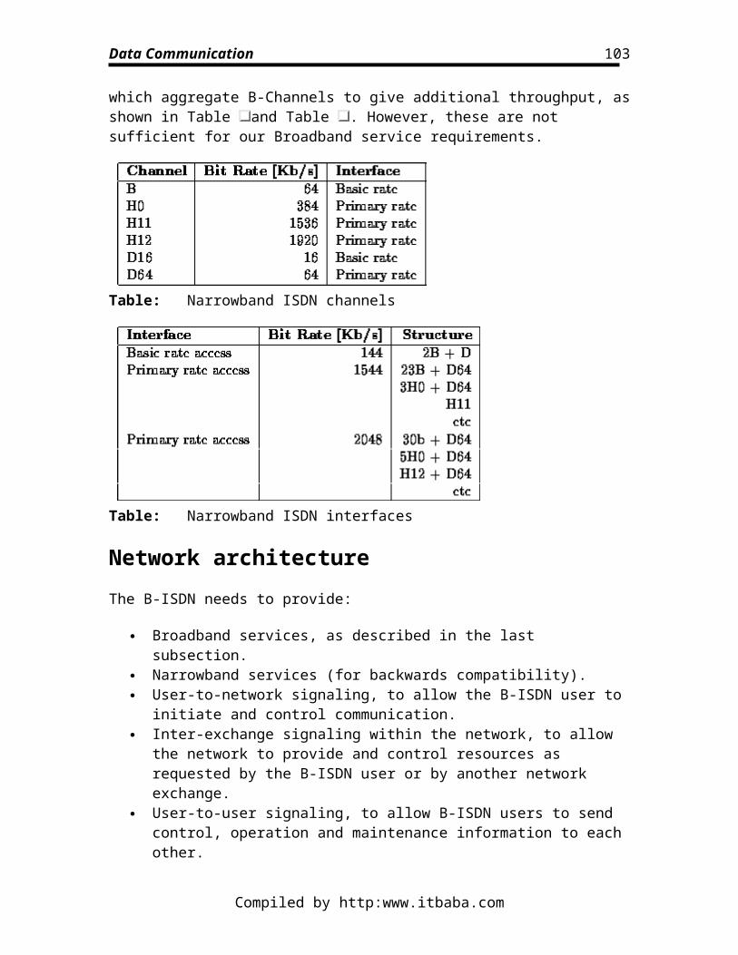
Data Communication

Figure: The main components of a switching element

In a matrix switch (or space division switch), the interconnection of network consists of a rectangular matrix of cross-points (Figure ). This is the simplest form of switch. Buffering can be used at the inputs, at the outputs, at the cross-points or at any three of these in combination.

Figure: A matrix switching element

Buffers placed at the inputs (Figure ) can be used to prevent collisions. If FIFOs are used, collisions will still occur if the messages at the head of the FIFOs are destined for the same port. Further, this will have the effect of blocking other messages in the queue. This problem can be overcome by the use of RAM buffers, but this may give rise to sequencing problems, and increase the complexity of the switching element.


103

http://www.cs.ucl.ac.uk/staff/S.Bhatti/D51-notes/node47.html#figmatrixswitchelement

http://www.cs.ucl.ac.uk/staff/S.Bhatti/D51-notes/node47.html#figipbmatrixswitchelement

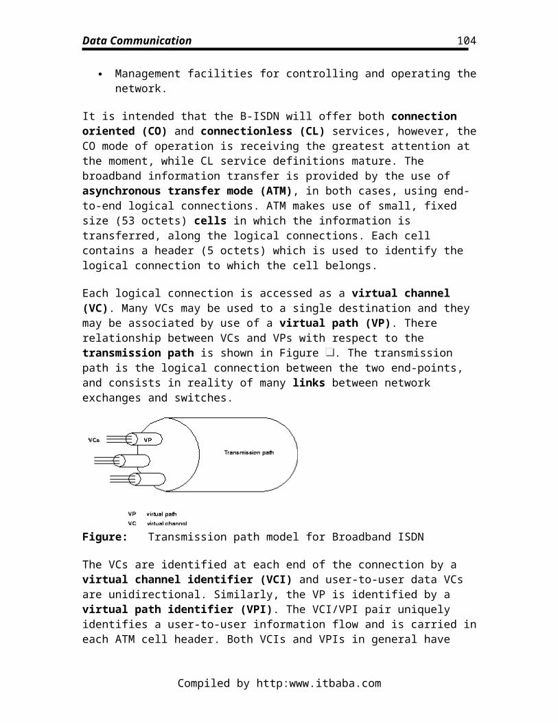
Data Communication

Figure: A matrix switching element with input buffers

Buffers placed at the outputs (Figure )can produce a non-blocking switching element if the switch is speeded up by a factor of N for a switch. If the speed up is not possible, then buffers must additionally be used at the inputs.

Figure: A matrix switching element with output buffers

Buffers can be placed at the cross-points of the interconnection matrix (Figure ), resulting in a Butterfly switching element. This requires logic to prevent collisions, based on some fairness and timeliness metric. A Butterfly switch may require a large increase in the complexity of the switching element, as each cross-point now requires memory.

Figure: A matrix switching element with buffers at the matrix cross-points


104

http://www.cs.ucl.ac.uk/staff/S.Bhatti/D51-notes/node47.html#figopbmatrixswitchelement

http://www.cs.ucl.ac.uk/staff/S.Bhatti/D51-notes/node47.html#figxpbmatrixswitchelement

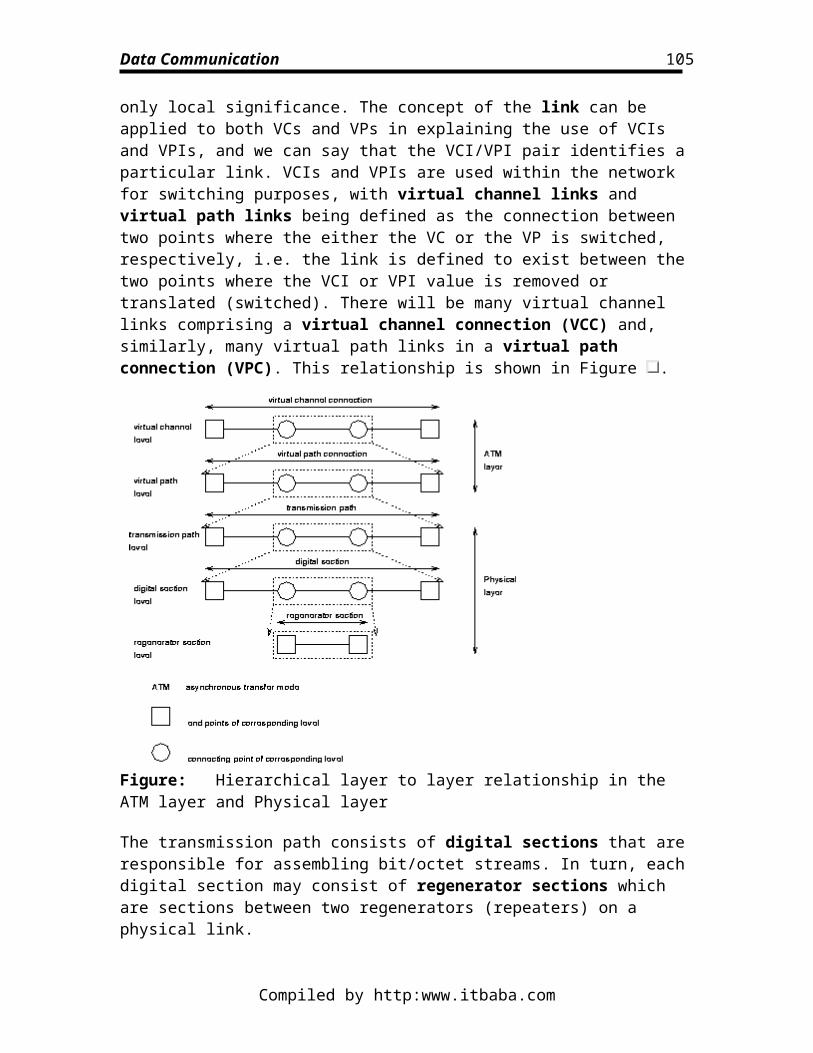
Data Communication

In the time slot interchange (TSI) technique (Figure ), the line is logically partioned, with respect to time, into regular time slots. Users on each side of the TSI switch are allocated a time slot. For two users, one on each side of the switch to communicate requires only that as the slot passes through the switch, its time slot is interchanged with that of the use on the other side. The size of this kind of switching element is limited by the memory access speed of the hardware. This switching element demonstrates an example of time domain multiplexing (TDM).

Figure: A time slot interchange switching element

Although single stage switching elements and switches are possible using one of these two, many useful switching fabrics can be realised with just these two switching elements used in multi stage switches. They are usually written as an enumeration of the order in which the stages are connected, with a S representing the matrix (space division switch), and a T representing a time division switch. Common fabrics are TST or STS.

In a central memory switching element (Figure ), the input controllers and output controllers are connected by central memory, which can be programmed to provide input and output buffering. This requires a highly parallel machine architecture for the purposes of memory access.

Figure: A central memory switching element

The interconnection network could also be arranged as a Bus-Type switching element, using a TDM bus (Figure . This is similar to a computer bus system. However, the bus


105

http://www.cs.ucl.ac.uk/staff/S.Bhatti/D51-notes/node47.html#figtsi

http://www.cs.ucl.ac.uk/staff/S.Bhatti/D51-notes/node47.html#figcmswitchelement

http://www.cs.ucl.ac.uk/staff/S.Bhatti/D51-notes/node47.html#figbusswitchelement

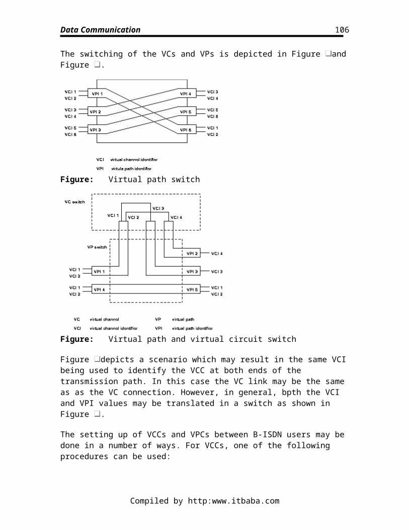
Data Communication

would have to be at least as fast as the sum of the speeds of its inputs to prevent messages being dropped.

Figure: A TDM bus switching element

A Ring-Type switching element (Figure ) passes round a time-slot that can be used by the input and output controllers connected to the ring, while having some of the constraints of the Bus-Type of switching element, the slot can be used several times in one cycle of the token.

Figure: A Ring-Type switching element

When a large number of (often identical) switching elements are connected together in a network, we have a multistage interconnection network (MIN). Probably the most famous MIN is the Delta Banyan network. This is a regular network of switching elements. An Delta Banyan switching fabric have the following useful properties:

1. They consist of identical switching elements. 2. They have the self-routing property, i.e. regardless of which input the message

arrives at, it will always be routed to the same input. Such routing requires bits of information.


106

http://www.cs.ucl.ac.uk/staff/S.Bhatti/D51-notes/node47.html#figringswitchelement

Data Communication

3. They consist of stages, with each stage having switching elements. 4. As they are regular networks, and have a simple interconnection pattern, they are

suited to VLSI techniques.

An example of a 4-stage Delta-Banyan network is given in Figure .

Figure: A Delta-2 4-Stage network

However, they are susceptible to blocking. This can be reduced by using a preceding distribution network (Figure ), but then this may cause sequencing problems without a complementary resequencing function at the outputs.

Figure: Structure of a distribution Banyan network

An alternative solution is to use a sorting network preceding the inputs, which orders the messages in a monotonous sequence, dependent on its destination output line. To prevent blocking, a trap network is placed after the sorting network, which feeds back messages with the same destination. Any fed back messages receive priority through the sorting network, in order to preserve sequencing. An example of such a network is the Batcher Banyan network.


107

http://www.cs.ucl.ac.uk/staff/S.Bhatti/D51-notes/node47.html#figd2network

http://www.cs.ucl.ac.uk/staff/S.Bhatti/D51-notes/node47.html#figdistbanyan

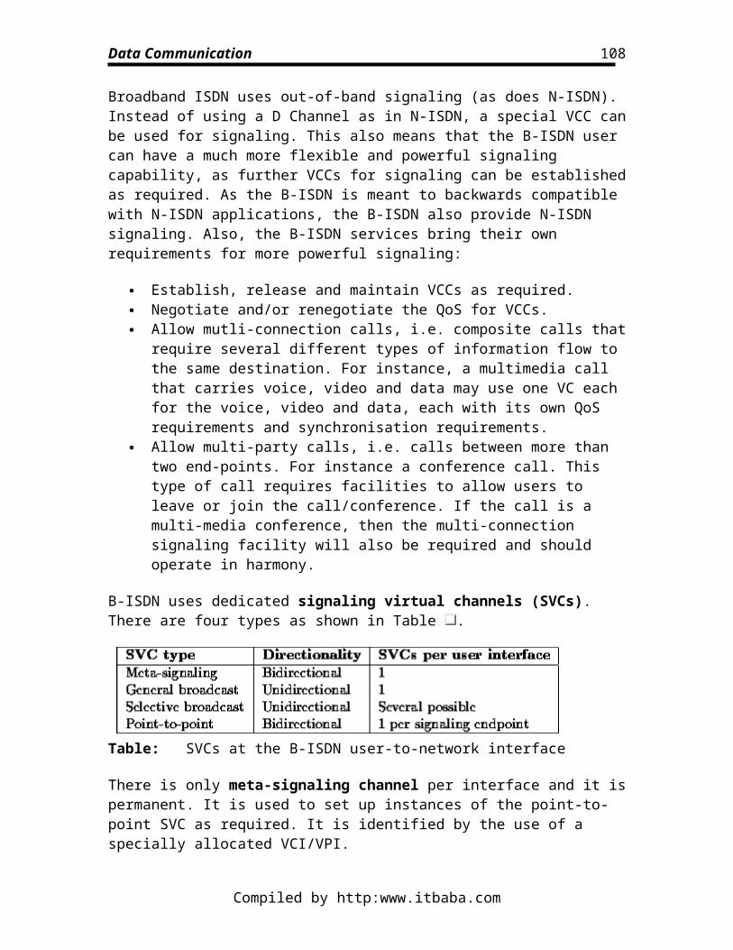
Data Communication

Figure: Structure of a sort-trap Banyan network

Switching services in networksOne of the most common uses of switching is in the private automatic branch exchange (PABX). A PABX is a local switch that performs a similar function to a switch in a PSTN, however it is does not use the PSTN, saving on costs and making communication in an office environment more efficient. In a company or organisation, much of the communication is voice. This means that, until recently, much of the PABX equipment was based on carrying analogue, limited bandwidth signals. If data switching is required for computer equipment, most institutions also employ some sort of LAN arrangement for electronic messaging and other such data services. However, as people realise the need for integration of services such as data, voice and video, increasing number of PABXs are being produced that employ digital switching techniques, capable of switching data, as well as voice and video that has undergone analogue to digital conversion (ADC). Such PABXs are also know as private digital exchanges (PDXs). PDXs can also offer additional services that may not have been possible in the analogue PABXs, such as call forwarding, call redirection, voice store-and-forward, etc.

Although the integration of voice and data using only one network via PDXs seems a natural step to take, it requires careful planning, and the management or corporate structure often assigns communications needs and data needs to different groups within in a company, so maintaining the separation between these services. Also, in an environment where there may be much data traffic with a very dynamic and unpredictable traffic profile, it may be unwise to switch voice traffic with data in case voice suffers at the cost of high bursts of data (e.g. UCL.CS!)

Another reason is that many data LANs are bus based - Ethernet remains the most widely used LAN environment - while the PDX based approach is naturally a star topology. With a LAN such as Ethernet, there is inherently a CL mode of operation while PDXs are circuit switches. It is likely that if PDXs are incorporated in to such a LAN environment they will be used to interconnect LAN segments.

Circuit switching will continue in widespread use all over world -- the world's telephone networks are circuit switched. Data requirements are ofted of a bursty nature and this is often because the exchange of data, unlike most phone calls, can often have very different data rates depending on direction. For instance, a user querying a database will probably make, for instance, simple menu choices which will result in the database providing much data in answer to his/her queries. This kind of data transfer is best suited to packet data, and can be facilitated by a packet switching exchange (PSE). PSEs switch data by considering the header data provided as part of each packet.


108

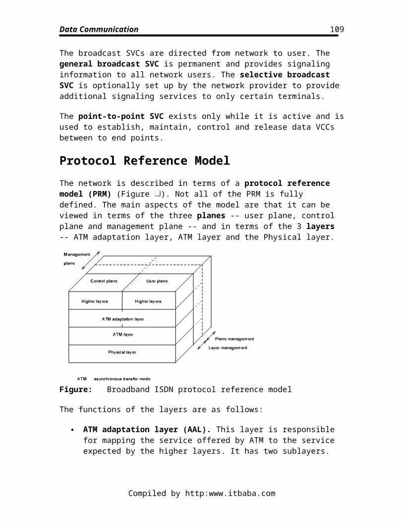
Data Communication

PSEs can also provide another service, that of virtual circuits (VC), each VC being referenced by a number called the virtual circuit identifier (VCI). When a user requires this service, a call request containing the address of the destination and a VCI is sent to the PSE. The destination, on accepting the call, assigns another VCI to the call request and forwards it. VCIs only have local significance. When the call request reaches the destination, a VC is said to exist between the two end-points. The VC maybe set up through a route that has many PSEs, although this is transparent to the end-points. Such a packet switched network is the X.25 network.

For the future, many people are looking to B-ISDN to provide integrated services - voice, video and data on one network using ATM. ATM switching can introduces new problems, not least the speed at which the switching must be achieved to maintain sufficient QoS. It seems likely that ATM switching will use the self-routing capabilities of Delta Banyan type switches. The main restriction in ATM switching is the electronic equipment that is required to process the optical signal. The optical signal must be converted to an electronic signal, processed, and then converted back to an optical signal from the electronic signal. Although CMOS, BiCMOS and ECL techniques can achieve Mb/s rates this may not be sufficient for the future Gb/s rates. GaAs technology may improve the situation but it seems that there will not be any significant progress until optical switching can be used. This may make it possible to fully exploit wave division multiplexing (WDM) or better coherent optical transmission techniques in modulation and switching.

High Speed NetworksUse of LANs is now common place in commercial, research, government and educational establishments. The evolution of hardware over the past decade has resulted in inexpensive solutions to interfacing computer systems to networks such as Ethernet and Token Ring. Such systems can typically offer around 10Mb/s on the shared media. Further, the ISDN is available widely in Britain and in many places in Europe and it is now possible to buy hardware that will allow access to the ISDN from a desktop machine.

The technology explosion has two important consequences:

Increase in the processing power available on the desktop. It is possible to go to a high street shop and buy a PC with hardware that can offer facilities for real-time conferencing across a LAN, or perform simulations in real-time.

A diversity of software wanting to make use of the increased processing power and available network capacity. As the hardware has become more capable so the applications designers have began to try and offer increasingly sophisticated services. Whereas LANS were initially used to provide access to, say, mailboxes or maybe a shared printer, we found now a host of services requiring the use of the network to provide real-time distributed services, for instance a distributed database or a network file service. Additionally,


109

Data Communication

applications that make higher demands from the network are also becoming very popular -- for example multimedia conferencing and computer supported cooperative work (CSCW).

As well as network hungry applications resulting in increased network load, we find that there are now few computer installations that are not networked -- virtually gone is the day of a stand alone PC used by a single person. So not only has the demand for network capacity increased per user but the number of users all contending for the same piece of LAN has increased.

To try and rationalise on the use of the available network capacity within an office or a site wide LAN, sites will often split the network up into segments. These segments are connected to a backbone network by use of bridges. The use of segments and bridges helps to localise traffic, so there is effectively less contention for the media compared to the case where there is only one segment. Further organisational changes like replication of data can also help to improve services for the user, but such schemes bring their own problems! While segmenting the network will help to create more localised traffic flows, the backbone may still need to contend with much inter-segment traffic.

Sometimes a user would simply like to have more network capacity available to him/her than the 10Mbp/s or so that, say, an Ethernet can offer, and if segments and bridges are used, the backbone needs to offer a greater capacity to cope with the many segments attached to it.

In this section we discuss some of the mechanisms of various high speed technologies that can bring 100Mbp/s and more to the LAN environment. Some of the technologies discussed here can be used to interconnect LANs over large public areas such as a town or city, and so are also referred to as metropolitan area networks (MANs).

Medium access control at high data rates Fibre Distributed Data Interface (FDDI) Distributed Queue Dual Bus (DQDB) High Performance Parallel Interface (HIPPI) 100Base-VG ATM LANs

Medium access control at high data ratesProbably the most common form of LAN medium access control (MAC) is carrier sense multiple access/collision detect (CSMA/CD), which is based on the use of a shared-bus network. We consider in this section why it is not feasible simply to run this kind of network 'faster' to get a higher throughput. Consider the following definitions for


110







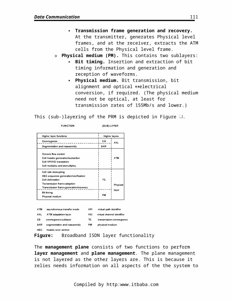
Data Communication

the propagation delay, , and in a MAC layer frame being transmitted and the time taken to transmit a MAC layer frame, :

where:

¯ D separation of transmitter and receiver [m]

V the velocity of propagation [m/s]

the number of bits in the frame

R the link bit rate [b/s]

maximum time taken to detect a collision [s]

CSMA/CD networks work well provided that A is small, i.e. the propagation delay is small compared to the time required to transmit the frame. This is necessary in order to detect collisions during transmission. The maximum time that a node on a CSMA/CD

network must wait to detect a collision is and so (from equations , and ) we see that 2A is the fraction of our frame that will be transmitted before a collision is

detected. Hence, if is much less than then there is not much time wasted when a

collision is detected. If we consider a 2.5Km bus and take m/s, then

s. So, in considering the detection of collisions, let us take a mean frame size of, say, 10 000 bits. Table summarises information concerning collision detection as the bit rate of the link increases.

Table: Collision detection data for a 2.5Km CSMA/CD bus (10 000 bit frame)


111

http://www.cs.ucl.ac.uk/staff/S.Bhatti/D51-notes/node50.html#equTp

http://www.cs.ucl.ac.uk/staff/S.Bhatti/D51-notes/node50.html#equA

http://www.cs.ucl.ac.uk/staff/S.Bhatti/D51-notes/node50.html#equTc

http://www.cs.ucl.ac.uk/staff/S.Bhatti/D51-notes/node50.html#tblcdframesize

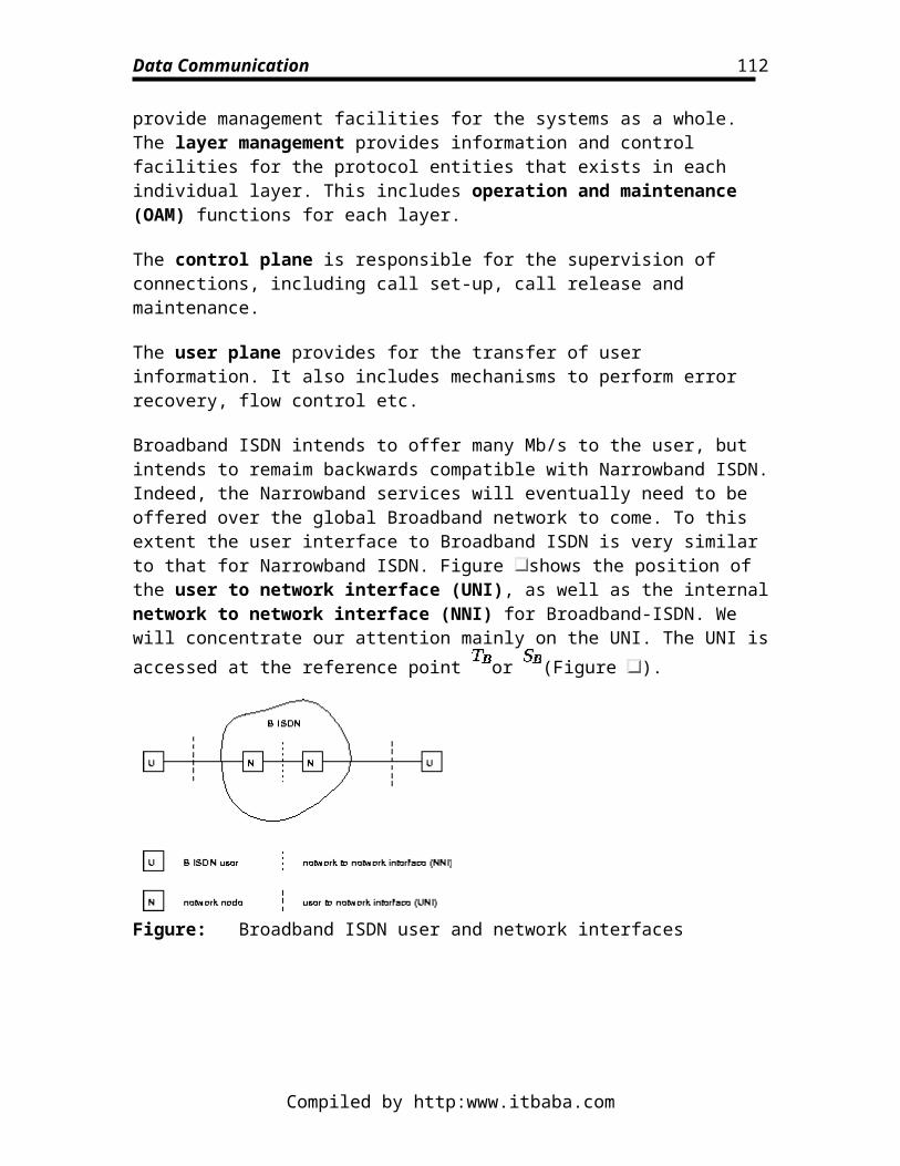
Data Communication

Table shows us that it is possible for the whole frame to have been transmitted before we can expect to detect a collision. This is obviously unacceptable. A solution to this problem might be to insist on an increasingly larger minimum frame size for higher transmission rates and longer cable lengths, but this is wasteful of network capacity. It is for these reasons that high speed networks -- both LANs and MANs -- must use other MAC methods.

Fibre Distributed Data Interface (FDDI)The fibre distributed data interface (FDDI) is a token based technology using fibre optical links. The FDDI specification defines the use of OSI layers 1 and 2 (Physical layer and Data Link layer). Some characteristics of FDDI are given in Table . FDDI's operation is similar to that of token ring.

Table: Some characteristics of FDDI

Dual counter-rotating rings are used to improve reliability. The rings are labelled the primary ring and the secondary ring. Stations attached to the FDDI may be connected to both rings -- dual attach stations (DASs) -- or only to the primary ring -- single attach station (SASs). Although, the stations are logically attached in a ring, the physical connection is more conveniently realised in a hub-star fashion by using wiring concentrators.

The FDDI may be used as a LAN, but is more often used as a backbone and so most of the attached stations will be bridges that are dual attached.

In a token ring, the single active ring monitor encodes the clock signal into the token that it generates, using Manchester encoding. However, for a 100Mb/s rate, Manchester encoding requires 200Mbaud signalling rate. So in an FDDI, NRZI coding is used (signal transition when a 1 is transmitted and no transition when a 0 is transmitted) and all stations have their own local clock which is used in data transmission. When receiving frames, stations synchronise using the incoming signal. The physical interface is depicted in Figure .


112

http://www.cs.ucl.ac.uk/staff/S.Bhatti/D51-notes/node50.html#tblcdframesize

http://www.cs.ucl.ac.uk/staff/S.Bhatti/D51-notes/node51.html#tblfddi

http://www.cs.ucl.ac.uk/staff/S.Bhatti/D51-notes/node51.html#figfddiinterface

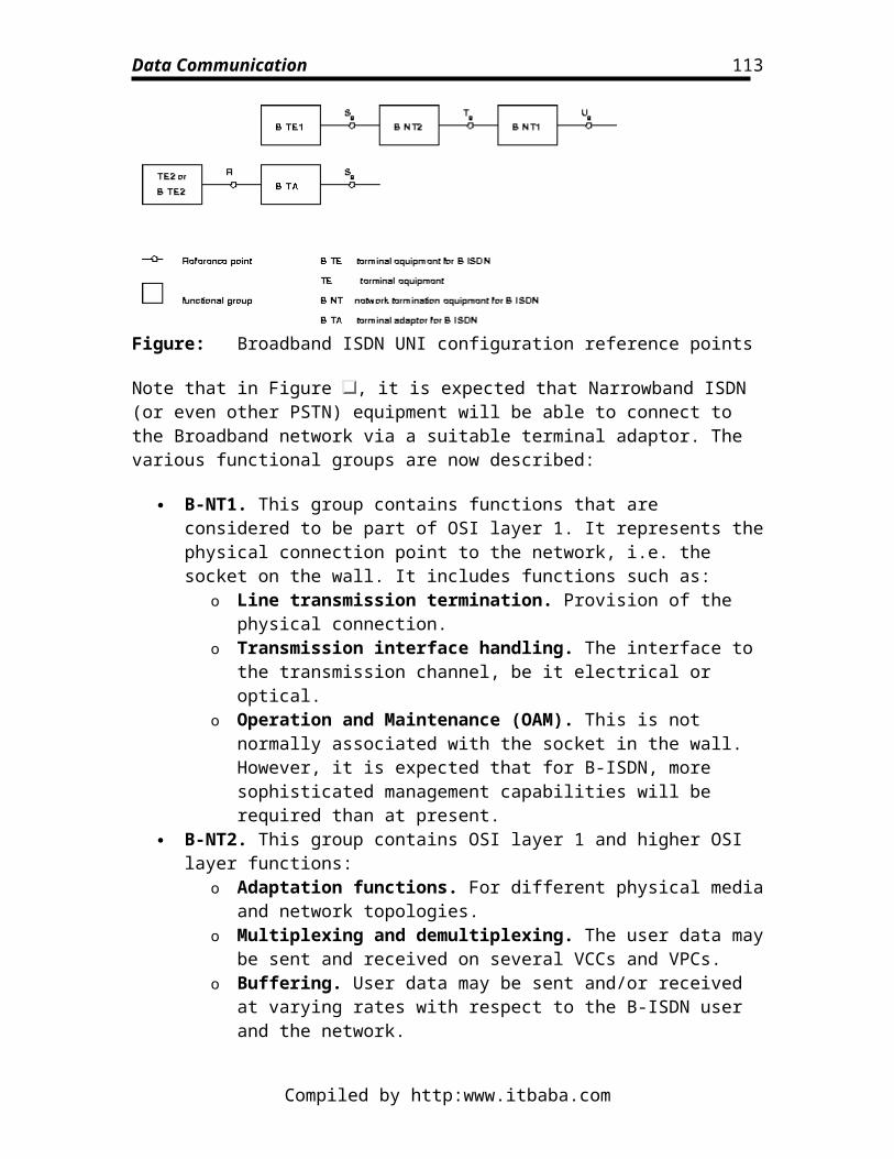
Data Communication

Figure: Schematic of FDDI physical interface

The 4B/5B encoder takes each group of 4 bits and replaces them with a 5-bit symbol (Table ), and the 4B/5B decoder performs the reverse operation. The use of 4B/5B coding and NRZI ensures a signal transition every 2 bits. The latency buffer is where 2 5-bit symbols are used to give correct symbol boundary alingment.

Table: FDDI 4B/5B data symbols


113

http://www.cs.ucl.ac.uk/staff/S.Bhatti/D51-notes/node51.html#tblfddidatacodes

Data Communication

Table: FDDI control code symbols

The FDDI frame formats are shown in Figure . The various fields are as follows (the various control symbols are given in Table ):

Preamble (PA): 16 (or more) IDLE symbols. Causes line signal changes every bit to ensure receiver clock synchronisation at the beginning of a frame.

Start delimiter (SD): the 2 symbols J and K are used to show the start of the frame and also to allow interpretation of correct symbol boundaries.

Frame control (FC): 2 symbols indicating whether or not this is an information frame or a MAC frame (e.g. the token), with some additional control information for the station identified by the DA.

Destination address (DA): 4 or 12 symbols identifying the destination station. 16 symbols are used for a full 48-bit MAC address, 4 symbols for a 16-bit local addressing mechanism. If the first bit of the (decoded) address is a 1 then this identifies a group address.

Source address (SA): 4 or 12 symbols identifying the source station. Information: this is usually set to about 9000 symbols (4500 decoded octets) in

length and is determined by the maximum length of time that a station can hold the token.

Frame check sequence (FCS): 8 symbols containing a 32-bit CRC. The FCS covers the fields FC, DA, SA, information and FCS.

End delimiter (ED): 1 or 2 T control symbols. Frame status (FS): 3 symbols which are a combination of R and S symbols

indicating if the frame has been seen by the destination station and if it has been copied by the destination station.


114

http://www.cs.ucl.ac.uk/staff/S.Bhatti/D51-notes/node51.html#figfddiframes

http://www.cs.ucl.ac.uk/staff/S.Bhatti/D51-notes/node51.html#tblfddicontrolcodes

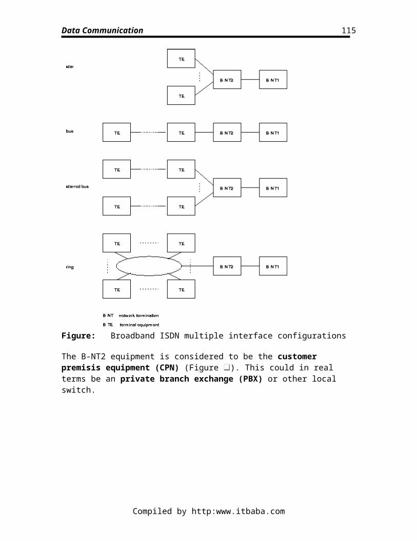
Data Communication

Figure: FDDI frame formats

The operation of FDDI is much the same as token ring. A station must be in possession of a token before it can transmit an information frame. Once it has seen the frame go around the ring it can the regenerate the token allowing someone else to transmit. However, the potentially large size of the FDDI ring means that it has a higher latency than token ring and so more than one frame may be circulating around the ring at a given time. The physical interface will then repeat the PA, SD, FC and DA filed before it nows if this is its own frame which it should remove from the ring. If this occurs, the station stops sending any more of the frame and instead sends out IDLE symbols until it receives an SD indicating another frame. This will lead to many frame fragments around the ring which should be removed by receiving stations.

All stations also keep a note of the token rotation time (TRT) which is the time elapsed since the station last saw the token. As the load on the FDDI network this time will increase. The TRT can be compared to a preset value called the target token rotation time (TTRT) to allow a priority operation scheme: only priority frames can be transmitted if the TRT is greater than the TTRT.

A timer called the token hold timer (THT) also controls the normal transmission of data. When a station receives the token it transfers the TRT to the THT which starts to count down. The station can then continue to transmit frames as long as the THT remains greater than the TTRT. In fact the THT determines the maximum number of octets/symbols that can be sent in one FDDI frame, as the the THT determines the maximum time that a station can remain transmitting data.

FDDI is a connectionless system and is designed for data purposes only. FDDI II is an evolution of FDDI which can be seen as a superset of FDDI. It was developed a standards project that proposed adding isochronous transmission services to FDDI so that it was possible to support real-time applications such as multimedia. The proposal includes a mechanism for dividing the the 100Mb/s into 16 channels, each of which would be allocated for a certain use, e.g.\ video, bursty data, etc. However, because existing FDDI hardware would be unable to have plug-in upgrades and with the advent of ATM LANs and DQDB, this option of FDDI may not be so heavily deployed.


115

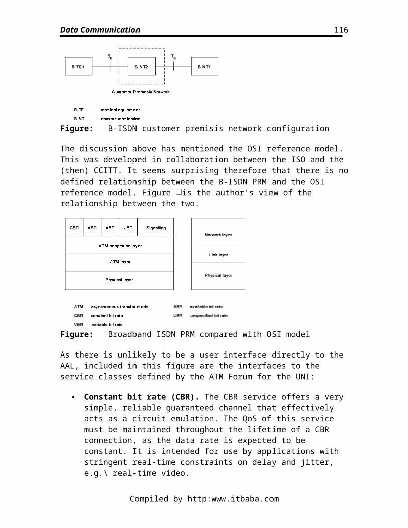
Data Communication

Distributed Queue Dual Bus (DQDB)The distributed queue dual bus (DQDB) network uses a different kind of MAC method based on the use of a distributed queuing algorithm called queued-packet distributed-switch (QPSX) and a slotted ring arrangement. It uses two unconnected unidirectional buses, which are normally implemented as a series of point-to-point segments. DQDB also expects the use of optical fibre links. Some of the characteristics of DQDB are given in Table .

Table: Some characteristics of DQDB

The DQDB LAN or MAN transports data in fixed size cells, which happen to look very much like ATM cells (Figures and ). However, as DQDB offers a MAC service, the MAC frame may need to be segmented into several cells before transmission (Figure ). The cell structure for DQDB is almost identical to that of an ATM cell. This similarity between the cell structure has been made so that the DQDB will be compatible with B-ISDN.

Figure: A DQDB cell


116

http://www.cs.ucl.ac.uk/staff/S.Bhatti/D51-notes/node52.html#tbldqdb

http://www.cs.ucl.ac.uk/staff/S.Bhatti/D51-notes/node52.html#figdqdbcell

http://www.cs.ucl.ac.uk/staff/S.Bhatti/D51-notes/node52.html#figdqdbcellheader

http://www.cs.ucl.ac.uk/staff/S.Bhatti/D51-notes/node52.html#figdqdbmacsegment

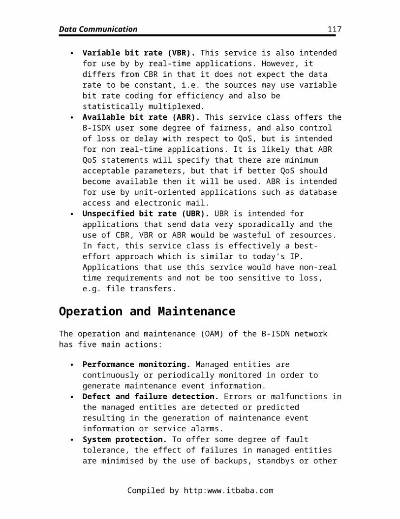
Data Communication

Figure: A DQDB cell header

Figure: MAC frame segmentation in DQDB

A DQDB cell differs from an ATM cell in its header and its payload. In the header of the DQDB cell there is no virtual path identifier (VPI) and the virtual channel identifier (VCI) has an additional 4 bits. The first 8 bits of the DQDB header form an access control field (ACF) (in ATM this is the first 8 bits of the VPI). Also, the next 4 bits (the final 4 bits of the VPI in ATM) form the first 4 bits of the VCI.

Also, the cell payload is structured:

Segment type (ST): identifies the cell as one of the following: o single segment: only this segment (no MAC fragmentation was required). o first segment: the first cell of a segmented MAC frame; o intermediate segment: the intermediate cells in a fragmented MAC

frame. o last segment: the final cell of a segmented MAC frame>

Message identifier (MID): the MID is the same for all DQDB cells from the same MAC frame. This allows the identification of intermediate segments.


117

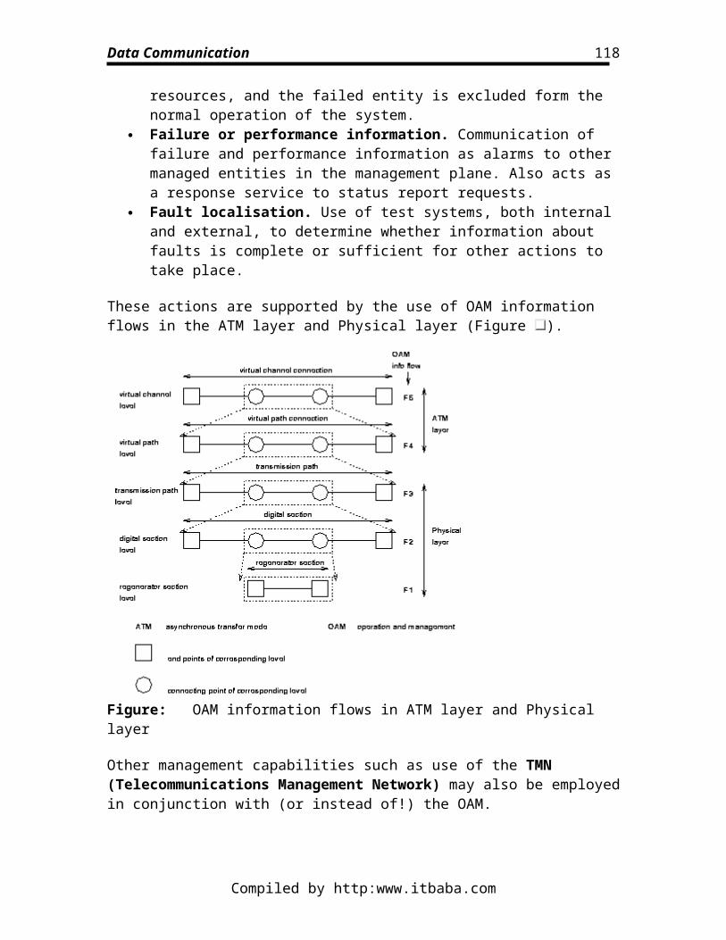
Data Communication

Information: (part of) the MAC frame contents. Length (LEN): the length of the information field. CRC: covering everything the whole cell payload.

The cell header contains the following information:

Access control field (ACF): this contains the BUSY and REQUEST bits that are used in the operation of the QPSX mechanism. The BUSY bit indicates the the slot is in use. The REQUEST bit is set in a slot by a node that is waiting to transmit.

Virtual channel identifier (VCI): This is not used in a DQDB MAN as there are no logical connections which require multiplexing -- the ST and MID fields in the payload are used instead. In a DQDB LAN with a private UNI, there is the possibility for applications to make use of this field.

Payload type (PT): same as ATM. Cell loss priority (CLP): same as ATM. Header error control (HEC): CRC for the header.

A DQDB network is comprised of two buses that transmit cells in opposite directions and each node is connected to both buses. The connections are normally point-to-point, but are often depicted in the tapped-bus type configuration as shown in Figure . Both these buses always have a constant number of slots circulating on them. A slot on one bus is copied to the other.


118

http://www.cs.ucl.ac.uk/staff/S.Bhatti/D51-notes/node52.html#figdqdboperation

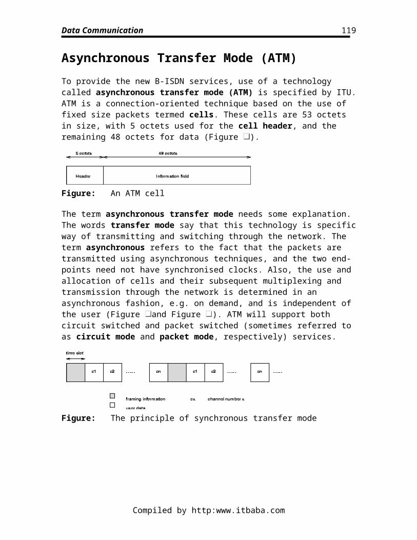
Data Communication

Figure: The operation of a DQDB network

The way that the DQDB network operates is by setting up a notion of a distributed queue at each node. This is done by using a counter -- REQUEST counter (RC) -- that records how many nodes are waiting to transmit ahead of this node in the queue. Consider Figure

which shows a node on the DQDB network. Only the inputs from the two buses to the node are shown, for simplicity. By ahead in the queue we mean any nodes upstream (relative to the flow of cells/slots) from this node. The count of waiting nodes is incremented by counting any set BUSY bits in passing slots on Bus A. The count is decremented by seeing any set REQUEST bits on Bus B.

For this node, we will consider what happens when it wishes to transmit on Bus A. Firstly, it waits for a passing slot on Bus B with an available REQUEST bit, which it then sets to indicate it is waiting to transmit. It then transfers the RC value to a down counter (DC). DC now contains the number of nodes ahead of this node in the queue. DC is decremented by slots passing by with BUSY bits set, indicating slots/cells used by other nodes that are ahead in the queue. When DC becomes 0, then this node can transmit on


119

http://www.cs.ucl.ac.uk/staff/S.Bhatti/D51-notes/node52.html#figdqdbcounter1

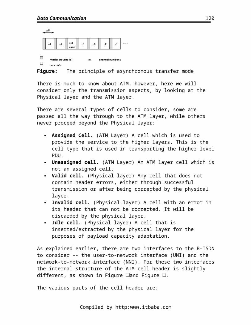
Data Communication

Bus A. Although we have only considered Bus A, an identical procedure is followed if the node wishes to transmit on Bus B.

Figure: DQDB node collecting queue information about Bus A

Figure: DQDB node waiting to send on Bus A

DQDB also has 4 priority transmission levels, which are also based around a distributed queue system using counters, i.e. each node effectively has 5 queues, with a RC and DC for each queue. The priority levels are indicated by 4 further REQUEST bits in the ACF in the cell header, labelled R1, R2, R3 and R4. The highest priority is R4. To cater for the priority levels, the behaviour of RC and DC must be modified as follows:

RC must count all request bits of its priority level or higher. DC decrements if an empty cell passes on Bus A, as this will be used by a waiting

node with a higher priority further downstream. DC increments if it sees a a REQUEST bit for a higher priority queue on Bus B.


120

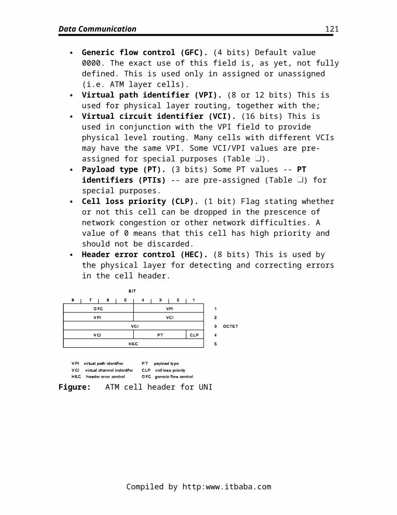
Data Communication

High Performance Parallel Interface (HIPPI)The high performance parallel interface (HIPPI) is a star-hub switch based technology for providing very high speed connectivity for short distances. The original HIPPI protocol specified the use of 50 copper twisted pairs to provide a uni-directional point-to-point link for a maximum length of 25 metres. HIPPI uses connections set up at very high speed through local switches. There is also work in progress to specify the use of HIPPI over fibre channel (an optical fibre based technology). Some of the characteristics of HIPPI are given in Table , with information about the fibre channel flavour of HIPPI given in brackets. The normal operating bit rate of HIPPI is 8000Mb/s.

Table: Some characteristics of HIPPI

A protocol suite is defined for the various functions to be performed in a HIPPI network (Figure ).

Figure: HIPPI protocol suite

The HIPPI physical layer (HIPPI-PH) is responsible for the electrical, mechanical and signalling aspects of HIPPI. The data is transferred in parallel normally as 32 bit words, but the cable can be doubled up (often called double wide HIPPI) to transfer 64 bit words


121

http://www.cs.ucl.ac.uk/staff/S.Bhatti/D51-notes/node53.html#tblhippi

http://www.cs.ucl.ac.uk/staff/S.Bhatti/D51-notes/node53.html#fighippisuite

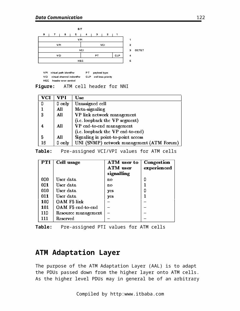
Data Communication

and so offer 1600Mb/s. As HIPPI has unidirectional links, upto four separate wires are required to support duplex 1600Mb/s data exchange. HIPPI uses a block parity based error control scheme at transmission time.

The HIPPI switching control (HIPPI-SC) function is responsible for setting up connections between HIPPI switches. The HIPPI network can be composed of many HIPPI switches (Figure ). The boxes marked as HIPPI device would be high performance machines (such as supercomputers), interworking units (for instance to B-ISDN) or intelligent peripheral devices. The switch control function uses information in the I-field of a HIPPI frame (see below). A HIPPI source requests a connection giving the relevant information in the I-field and the switch will try and make the connection to the destination, then data transfer can proceed, after which the connection is released. The control bits in the I-field and their affect on connection establishment is explained below. It is possible to get switches that can set up connections in less than one microsecond!

Figure: A LAN constructed using HIPPI switches

HIPPI specifies a framing protocol for transmitting information (Figure ). The unit of transmission for data is a burst of 256 words (32 bits or 64 bits). The I-field contains information that is used for switching by the hub(s) (Figure ). The various bits of the I-field are:

Locally defined (L): if this bit is set to one, it signifies that the rest of the I-field has locally (privately) defined format and not the standard format.

Width (W): if this bit is set it indicates that a double wide HIPPI connection (64 bit words) should be attempted. If the source or the destination can not support this, the connection request is rejected.

Direction (D): if this bit is set it indicates that the source and destination address bits should be swapped round. This provides a method for devices to simply route return messages, but is not useful when a LAN type arrangement is in operation such as that depicted in Figure .

Path selection (PS): determines how the I-field address information is treated. It can be treated as a 24 bit block which contains a series of port numbers that effectively define s route through a set of switches, or it can be used as two 12 bit


122

http://www.cs.ucl.ac.uk/staff/S.Bhatti/D51-notes/node53.html#fighippilan

http://www.cs.ucl.ac.uk/staff/S.Bhatti/D51-notes/node53.html#fighippiframing

http://www.cs.ucl.ac.uk/staff/S.Bhatti/D51-notes/node53.html#fighippiifield

http://www.cs.ucl.ac.uk/staff/S.Bhatti/D51-notes/node53.html#fighippilan

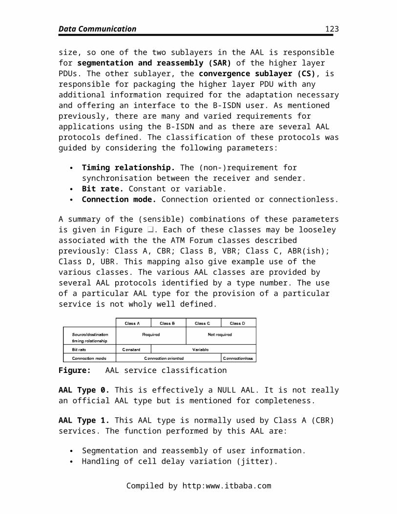
Data Communication

addresses, as depicted in Figure . The former mode is called source route mode and the latter logical address mode.

Camp on (C): is set, this bit instructs the switch not to reject the connection if the destination is busy, but to wait until the destination is free and then re-attempt the connection.

Source/Destination address: this information in logical address mode is often encoded as a 6 bit switch number and a 6 bit port number.

Figure: HIPPI data framing hierarchy

Figure: HIPPI data frame I-field

The HIPPI link encapsulation (HIPPI-LE) offers an interface that supports IEEE 802.2 Logical link PDUs, i.e. it looks like a CSMA/CD or token-bus/ring LAN but 80/160 times as fast! This provides a way for other standard technologies to be used over HIPPI, e.g. the Internet Protocol suite, IP, UDP and TCP.

The HIPPI fibre channel (HIPPI-FC) interface is still under development, but when completed, hopes to offer a increased capabilities, as shown by the bracketed information in Table .

The HIPPI intelligent peripheral interface (HIPPI-IPI) will allow high speed computer controlled peripherals (such as optical disc drives) and the HIPPI-FC developments intends to add support for the small computer systems interface (SCSI) command set.


123

http://www.cs.ucl.ac.uk/staff/S.Bhatti/D51-notes/node53.html#fighippiifield

http://www.cs.ucl.ac.uk/staff/S.Bhatti/D51-notes/node53.html#tblhippi

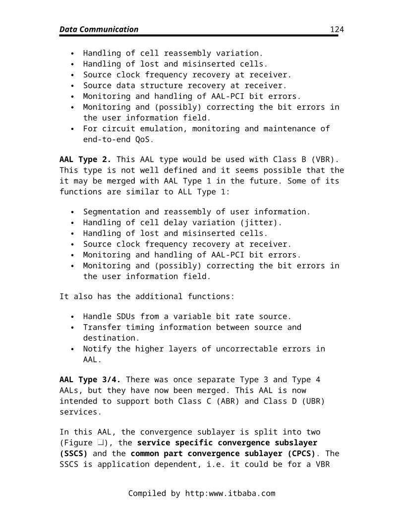
Data Communication

100Base-VG100Base-VG is a hub-star topology system that uses a round-robin policy for allowing connected stations to transmit on the network. It is not intended (or has any future plans) for use over long distances as is the previously discussed technology. It is intended for use by small local workgroups. Also, it is intended to work over existing 10BaseT twisted pair voice grade cabling now being used for 10Mb/s CSMD/CD or Ethernet networks, so one of its main strengths is that it is relatively cheap to install. Some of the characteristics of 100BaseVG are given in Table .

Table: Some characteristics of 100Base-VG

The operation of the network is very simple. When a station wishes to transmit, it requests network access by using a tone of a certain frequency. When access is granted, the station can transmit its frame and also receive a frame. It is only allowed to transmit and receive one packet at a time. An acknowledgement is by way of a tone issued from the hub. Apart from this special signalling protocol, it is essentially a LAN type MAC service. Multicast and broadcast is handled by a store-and-forward mechanism in the switch and a special signalling tone directed from the hub/switch to the station. A typical set-up is depicted in Figure .

Figure: An example 100Base-VG hub set-up


124

http://www.cs.ucl.ac.uk/staff/S.Bhatti/D51-notes/node54.html#tbl100basevg

http://www.cs.ucl.ac.uk/staff/S.Bhatti/D51-notes/node54.html#fig100basevghub

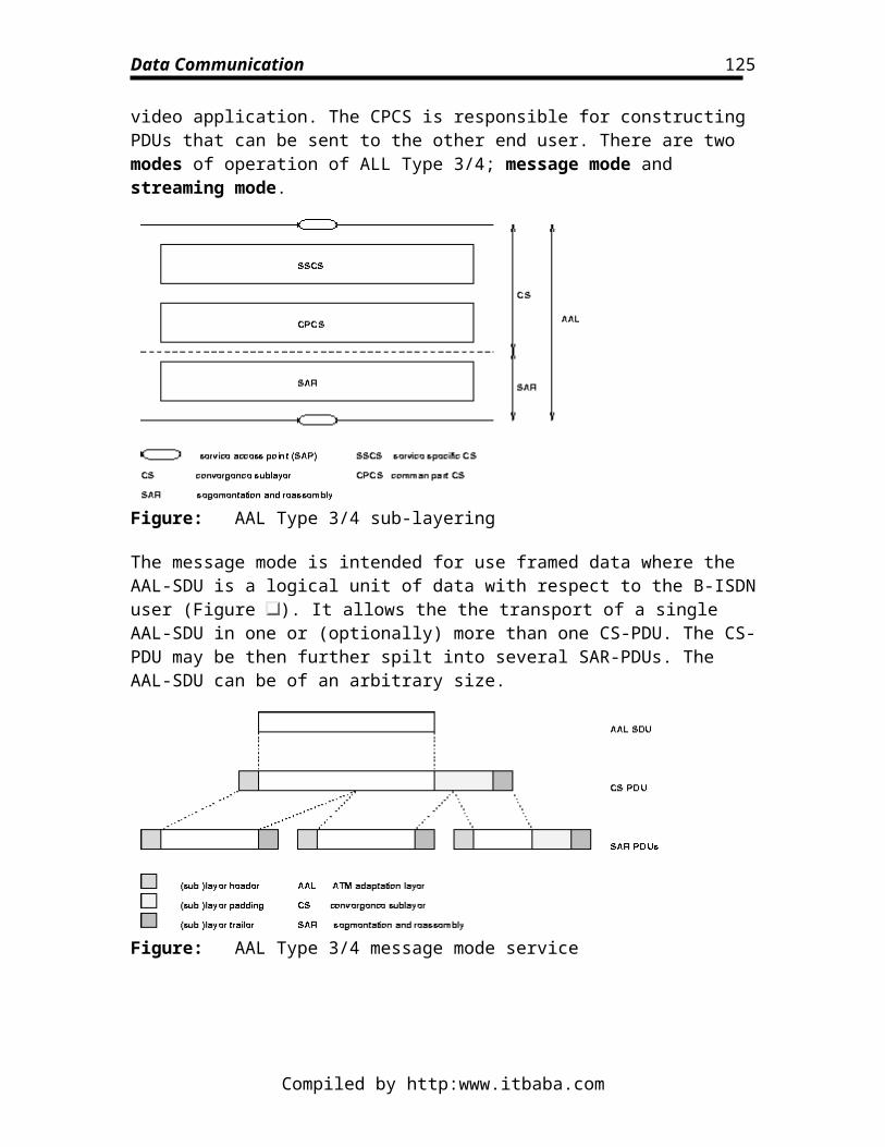
Data Communication

All stations are accessed in a round-robin fashion, thereby assuring a high degree of fairness with respect to network access. With such fairness, it is easy to evaluate the maximum access delay of this network and so it is very much suited for use by workgroups that make use of multi-media or real-time applications with stringent timing or synchronisation requirements.

The system also supports a single priority level, which modifies the round-robin arbitration behaviour by allowing priority access requests to preempt normal access requests.

Future plans for 100Base-VG include further support for multi-media applications but to offer a some guaranteed high bit rate logical channels by overlaying a connection management scheme over the basic network arbitration mechanism by introducing additional signalling procedures.

ATM LANsThe concept of ATM LANs (or local ATM (LATM) is very simple: use ATM switches to build a LAN and so allow users to have access extremely high network capacity. Such an ATM LAN may be as depicted in Figure . In fact, it is expected that this will be the most common usage of ATM at least in the near future. While there are no readily available B-ISDN services and much work is progressing on high throughput applications, there is a need for high speed reliable network environments for workgroups. Using ATM LANs also offer the advantage that the applications developed to use them may be used over DQDB MANs and any B-ISDN infrastructure as it appears.

Figure: An example ATM LAN configuration


125

http://www.cs.ucl.ac.uk/staff/S.Bhatti/D51-notes/node55.html#figatmlan

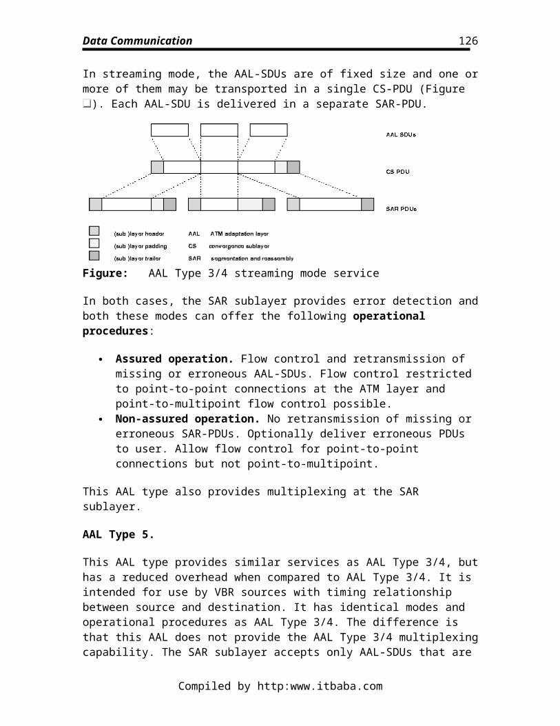
Data Communication

For such local use, the ATM forum have defined several low cost interfaces that can run at lower rates (e.g. 2Mb/s) and use existing wiring.

This concept can be extended further by saying that it is possible to bring high speed links to the desktop, e.g. 150Mb/s, and that this cab be exploited by peripherals directly. In a similar fashion to the HIPP-IPI interface, people are considering peripheral devices that connect to a desktop area network (DAN) that is effectively and extension of the desktop machine's back-plane bus. All the peripheral components, for example video cameras, disc drives, printers, etc., would be able to communicate with the processor or memory directly using ATM. This would mean that the peripherals could be located remotely or locally and this could be made transparent to the application, but also that any peripheral could easily be connected to the desktop machine via a high speed interface.


126

Documents

Lecture notes for M - Itbaba.comitbaba.com/ditnotes/data communication.doc · Web viewThere is considerable scope for confusion if the use of the words analogue and digital are not