Embed Size (px)
Citation preview

Lecture Notes
Statistical Mechanics
Alejandro L. Garcia
San Jose State University
PHYSICS 260 / Spring 2012

c⃝2012 by Alejandro L. Garcia
Department of Physics, San Jose State University, San Jose CA 95192-0106
Creative Commons Attribution- Noncommercial-Share Alike 3.0 United States License
Preface
These lecture notes should supplement your notes, especially for those of you (like myself) who are poor
note takers. But I don’t recommend reading these notes while I lecture; when you go to see a play you
don’t take the script to read along. Continue taking notes in class but relax and don’t worry about
catching every little detail. WARNING: THESE NOTES ARE IN DRAFT FORM AND
PROBABLY HAVE NUMEROUS TYPOS; USE AT YOUR OWN RISK.
The main text for the course is R. K. Pathria and Paul D. Beale, Statistical Mechanics, 3rd Ed.,
Pergamon, Oxford (2011). Other texts that will sometimes be mentioned and that you may want to
consult include: K. Huang, Statistical Mechanics, 2nd Ed., Wiley, New York (1987); F. Reif, Funda-
mentals of Statistical and Thermal Physics, McGraw-Hill, New York (1965); L.D. Landau and E.M.
Lifshitz, Statistical Physics, Addison-Wesley, Reading Mass. (1969).
Here is the general plan for the course: First review some basic thermodynamics and applications;
this is not covered in your text book but any undergraduate thermodynamics book should be suitable.
Given the entropy of a system, all other thermodynamic quantities may be found. The theory of
statistical ensembles (Chapters 1−4 in Pathria) will tell us how to find the entropy given the microscopic
dynamics. The theory of ensembles connects mechanics and thermodynamics.
The calculations involved in ensemble theory can be quite hard. We start with the easier non-
interacting systems, such as paramagnets, classical ideal gas, Fermion gas, etc., (Chapters 6 − 8) and
work up to interacting systems, such as condensing vapor and ferromagnets (Chapter 12− 13).
Most of statistical mechanics is concerned with calculating statistical averages but we briefly con-
sider the variation of microscopic and macroscopic quantities about their mean values as predicted by
fluctuation theory (Chapter 15). Finally we’ll touch on my own specialty, computer simulations in
statistical mechanics in Chapter 16.
Alejandro L. Garcia
1
Chapter 1
Thermodynamics
Equation of StateLecture 1
We consider thermodynamic systems as physical systems entirely described by a set of thermodynamic
parameters. Commonly used parameters include:
• pressure, P , and volume, V
• tension, τ and length, L
• magnetic field, H and magnetization, M
These parameters appear in pairs, the first being a generalized force and the second a generalized
displacement, with the product of the pair having the dimensions of energy. All these parameters are
well-defined by mechanics and are readily measured mechanically.
An additional thermodynamic parameter, temperature, T , is not a mechanical parameter; we defer
its definition for now. Rather than trying to be general, let’s say that our thermodynamic parameters
are P , V , and T , for example, if our system was a simple gas in a container.
An isolated system (no energy or matter can enter or leave the system) will, in time, attain thermo-
dynamic equilibrium. At thermodynamic equilibrium, the parameters do not change with time. Though
thermometers have been in use since the time of Galileo (late 1500’s) many concepts regarding temper-
ature were not well understood until much later. In the mid 1700’s Joseph Black used thermometers to
establish that two substances in thermal contact have the same at thermodynamic equilibrium. This is
counterintuitive — if metal and wood are at thermal equilibrium the metal still “feels colder” than the
wood. This misleading observation is due to the fact that our sense of touch uses conduction of heat
and thus is a poor thermometer.
The equation of state is the functional relation between P , V , and T at equilibrium (see Fig. 1.1).
An example of an equation of state is the ideal gas law for a dilute gas,
PV = NkT (Ideal gas only)
where N is the number of molecules in the gas and k (k = 1.38× 10⁻²³ J/K is Boltzmann’s constant.
Boltzmann’s constant does not have any deep meaning. Since the temperature scale was developed long
before the relation between heat and energy was understood the value of k simply allows us to retain
the old Kelvin and Celsius scales. Later we’ll see the theoretical justification for the ideal gas law in
the next chapter.
2

CHAPTER 1. THERMODYNAMICS 3
Figure 1.1: Point in state space on the equation of state surface
Figure 1.2: Path from points A to B in pressure-volume diagram
You should not get the impression that the equation of state completely specifies all the thermody-
namic properties of a system. As an example, both argon and nitrogen molecules have about the same
mass and the two gases obey the ideal gas law yet their molar heat capacities are very different (can
you guess why Ar and N2 are different?).
It follows from the equation of state that given V and T , we know P at equilibrium (or in general,
given any two we know the third).
First Law of Thermodynamics
Call U(V, T ) the internal energy∗ of our system (why don’t we write U(P, V, T )?). One way that the
energy can change is if the system does mechanical work. The work done by a system in going from
state A to B is,
∆WAB =
∫ VB
VA
P (V ) dV
since Work = Force × Distance = (Force/Area) × (Distance×Area) = (Pressure) × (Volume). Graph-
ically, the work done is the area under the path travelled in going from A to B as shown in Fig. 1.2.
The mental picture for this process is that of a piston lifting a weight as the system’s volume expands.
Notice that if the path between A and B is changed, ∆WAB is different; for this reason dW = P dV is
not an exact differential.
∗NOTATION: Pathria writes E(V, T ) instead of U(V, T ).
CHAPTER 1. THERMODYNAMICS 4
By conservation of energy,
U(VB , TB)− U(VA, TA) = ∆QAB −∆WAB
where ∆QAB is the non-mechanical energy change in going from A to B. We call ∆QAB the heat added
to the system in going from A to B. If A and B are infinitesimally close,
dU = dQ− dW = dQ− PdV (∗)
where dU is an exact differential though dQ and dW are not. This is the first law of thermodynamics,
which simply states that total energy is conserved.
The results so far are very general. If our mechanical variables are different, everything carries over.
For example, for a stretched wire the mechanical variables are tension τ and length L instead of P and
V . We simply replace P dV with −τ dL in equation (∗). Note that the minus sign comes from the fact
that the wire does work when it contracts (imagine the wire contracting and lifting a weight).
Example: For n moles of an ideal gas held at constant temperature T0 find the work done in going
from volume VA to VB .
Solution: The number of molecules in n moles is N = nNA where NA = 6.205×10²³ is Avogadro’s
number (not to be confused with Avocado’s number which is the number of molecules in a guaca-mole).
The ideal gas equation of state is
PV = NkT = (nNA)kT = nRT
where R = kNA = 8.31 J/(mol K) is the universal gas constant.
To find the work done, we solve,
∆WAB =
∫ VB
VA
P (V ) dV
Since the temperature is fixed at T0, then P (V ) = nRT0/V or
∆WAB = nRT0
∫ VB
VA
dV
V= nRT0 ln(VB/VA)
Note that on a different path we would have to know how temperature varied with volume, i.e., be
given T (V ) along the path.
Heat capacity
We define heat capacity, C, as
dQ = CdT
Specifically, the heat capacity at constant volume, CV , is
CV =
(∂Q
∂T
)V

CHAPTER 1. THERMODYNAMICS 5
and the heat capacity at constant pressure
CP =
(∂Q
∂T
)P
The heat capacity gives the amount of heat energy required to change the temperature of an object
while holding certain mechanical variables fixed. We also define the heat capacity per unit mass, which
is often called the specific heat, and the heat capacity per particle (e.g., cV = CV /N).
For liquids and solids, since their expansion at constant pressure is often negligible, one finds CP ≈CV ; this is certainly not the case for gases.
For any function f(x, y) of two variables, the differential df is
df =
(∂f
∂x
)y
dx+
(∂f
∂y
)x
dy (Math identity)
where the subscripts on the parentheses remind us that a variable is held fixed. Applying this identity
to internal energy
dU(T, V ) =
(∂U
∂T
)V
dT +
(∂U
∂V
)T
dV (∗∗)
If we hold volume fixed (i.e., set dV = 0) in this expression and in (*) then we obtain the result
dQ =
(∂U
∂T
)V
dT (constant V )
From the above,
CV =
(∂U
∂T
)V
This result is easy to understand since the change in internal energy equals the heat added when volume
is fixed since no work can be done if volume is fixed.
The heat capacity is important because given the equation of state and the heat capacity of a
system, all other thermodynamic properties can be obtained. This is proved in most thermodynamics
textbooks.
Joule’s Free Expansion Experiment
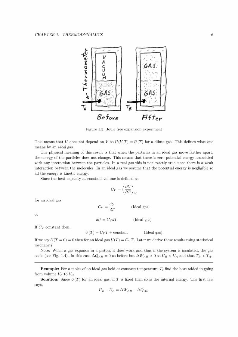
Let’s apply some of these results to a historically important experiment. Take a gas in an insulated
container as shown in Fig. 1.3.
Experimentally, one finds that TB = TA, that is, the temperature remains constant after the gas
expands to fill both sides of the container. If you were thinking that the gas would cool when it
expanded, I’ll explain the source of your confusion in a moment.
In the free-expansion, the gas does no work so, ∆WAB = 0. The system is insulated so no heat
enters or leaves, thus ∆QAB = 0. From first law, the internal energy U must remain constant.
From (∗∗) for constant U ,
0 =
(∂U
∂T
)V
dT +
(∂U
∂V
)T
dV (dU = 0)
Since the experiment shows that the temperature does not change on expansion, then dT = 0 and thus
for an ideal gas, (∂U
∂V
)T
dV = 0 (Ideal Gas)
CHAPTER 1. THERMODYNAMICS 6
Figure 1.3: Joule free expansion experiment
This means that U does not depend on V so U(V, T ) = U(T ) for a dilute gas. This defines what one
means by an ideal gas.
The physical meaning of this result is that when the particles in an ideal gas move farther apart,
the energy of the particles does not change. This means that there is zero potential energy associated
with any interaction between the particles. In a real gas this is not exactly true since there is a weak
interaction between the molecules. In an ideal gas we assume that the potential energy is negligible so
all the energy is kinetic energy.
Since the heat capacity at constant volume is defined as
CV =
(∂U
∂T
)V
for an ideal gas,
CV =dU
dT(Ideal gas)
or
dU = CV dT (Ideal gas)
If CV constant then,
U(T ) = CV T + constant (Ideal gas)
If we say U(T = 0) = 0 then for an ideal gas U(T ) = CV T . Later we derive these results using statistical
mechanics.
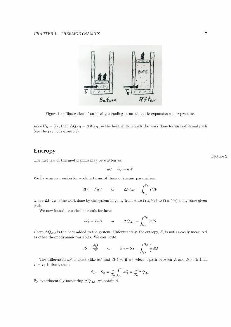
Note: When a gas expands in a piston, it does work and thus if the system is insulated, the gas
cools (see Fig. 1.4). In this case ∆QAB = 0 as before but ∆WAB > 0 so UB < UA and thus TB < TA.
Example: For n moles of an ideal gas held at constant temperature T0 find the heat added in going
from volume VA to VB .
Solution: Since U(T ) for an ideal gas, if T is fixed then so is the internal energy. The first law
says,
UB − UA = ∆WAB −∆QAB
CHAPTER 1. THERMODYNAMICS 7
Figure 1.4: Illustration of an ideal gas cooling in an adiabatic expansion under pressure.
since UB = UA, then ∆QAB = ∆WAB , so the heat added equals the work done for an isothermal path
(see the previous example).
EntropyLecture 2
The first law of thermodynamics may be written as:
dU = dQ− dW
We have an expression for work in terms of thermodynamic parameters:
dW = PdV or ∆WAB =
∫ VB
VA
PdV
where ∆WAB is the work done by the system in going from state (TA, VA) to (TB , VB) along some given
path.
We now introduce a similar result for heat:
dQ = TdS or ∆QAB =
∫ SB
SA
TdS
where ∆QAB is the heat added to the system. Unfortunately, the entropy, S, is not as easily measured
as other thermodynamic variables. We can write:
dS =dQ
Tor SB − SA =
∫ QB
QA
1
TdQ
The differential dS is exact (like dU and dV ) so if we select a path between A and B such that
T = T0 is fixed, then:
SB − SA =1
T0
∫ B
A
dQ =1
T0∆QAB
By experimentally measuring ∆QAB , we obtain S.

CHAPTER 1. THERMODYNAMICS 8
Figure 1.5: Carnot engine cycle in P − V diagram
But what if we cannot get from A to B along an isothermal path? Along an adiabatic path (no heat
added or removed) dQ = 0 so dS = 0. In general, we can build a path between any two points A and
B by combining isothermal and adiabatic paths and thus calculate SB − SA.
The entropy is important in that given S(U, V ) for a physical system, all other thermodynamic
properties may be computed. We derive and use this result when we develop statistical mechanics.
Third Law of Thermodynamics
The entropy is a function of the thermodynamic parameters so we may write it as S(T, V ). The third
law says:
S(T = 0, V ) = 0
that is, at zero Kelvin the entropy is zero. Thus, we can find the entropy for arbitrary T and V by
computing:
S(T, V ) =
∫ (T,V )
(T=0,V )
dQ
T
along any convenient path. There are many deep meanings to the third law and I encourage you to
plunge in and read about them on your own.
Engines and Refrigerators
A heat engine is described by a closed cycle in a P − V diagram for which the enclosed area (i.e., the
work done) is positive (contour loop is clockwise). If the loop is counterclockwise we have a refrigerator.
Call the heat added in a cycle Q+ and the work done W ; we define engine efficiency as η = W/Q+,
that is, the fraction of the heat added that is converted into work.
An important example is a Carnot engine. In a Carnot engine the cycle consists of a pair of
isothermal paths and a pair of adiabatic paths (see Fig. 1.5).
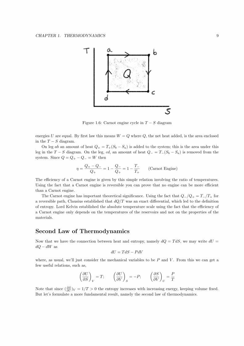
Notice that the Carnot cycle is a rectangle in the T − S diagram (see Fig. 1.6). The area enclosed
in the P − V diagram is the work done. Since the cycle is a closed loop, our final and initial internal
CHAPTER 1. THERMODYNAMICS 9
Figure 1.6: Carnot engine cycle in T − S diagram
energies U are equal. By first law this means W = Q where Q, the net heat added, is the area enclosed
in the T − S diagram.
On leg ab an amount of heat Q+ = T+(Sb − Sa) is added to the system; this is the area under this
leg in the T − S diagram. On the leg, cd, an amount of heat Q− = T−(Sb − Sa) is removed from the
system. Since Q = Q+ −Q− = W then
η =Q+ −Q−
Q+= 1− Q−
Q+= 1− T−
T+(Carnot Engine)
The efficiency of a Carnot engine is given by this simple relation involving the ratio of temperatures.
Using the fact that a Carnot engine is reversible you can prove that no engine can be more efficient
than a Carnot engine.
The Carnot engine has important theoretical significance. Using the fact that Q−/Q+ = T−/T+ for
a reversible path, Clausius established that dQ/T was an exact differential, which led to the definition
of entropy. Lord Kelvin established the absolute temperature scale using the fact that the efficiency of
a Carnot engine only depends on the temperatures of the reservoirs and not on the properties of the
materials.
Second Law of Thermodynamics
Now that we have the connection between heat and entropy, namely dQ = TdS, we may write dU =
dQ− dW as
dU = TdS − PdV
where, as usual, we’ll just consider the mechanical variables to be P and V . From this we can get a
few useful relations, such as,(∂U
∂S
)V
= T ;
(∂U
∂V
)S
= −P ;
(∂S
∂V
)U
=P
T
Note that since ( ∂S∂U )V = 1/T > 0 the entropy increases with increasing energy, keeping volume fixed.
But let’s formulate a more fundamental result, namely the second law of thermodynamics.
CHAPTER 1. THERMODYNAMICS 10
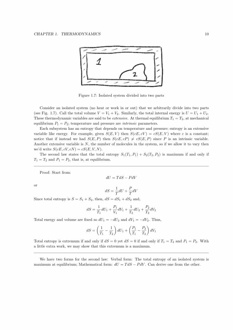
Figure 1.7: Isolated system divided into two parts
Consider an isolated system (no heat or work in or out) that we arbitrarily divide into two parts
(see Fig. 1.7). Call the total volume V = V1 + V2. Similarly, the total internal energy is U = U1 + U2.
These thermodynamic variables are said to be extensive. At thermal equilibrium T1 = T2, at mechanical
equilibrium P1 = P2; temperature and pressure are intrinsic parameters.
Each subsystem has an entropy that depends on temperature and pressure; entropy is an extensive
variable like energy. For example, given S(E, V ) then S(cE, cV ) = cS(E, V ) where c is a constant;
notice that if instead we had S(E,P ) then S(cE, cP ) = cS(E,P ) since P is an intrinsic variable.
Another extensive variable is N , the number of molecules in the system, so if we allow it to vary then
we’d write S(cE, cV, cN) = cS(E, V,N).
The second law states that the total entropy S1(T1, P1) + S2(T2, P2) is maximum if and only if
T1 = T2 and P1 = P2, that is, at equilibrium.
Proof: Start from:
dU = TdS − PdV
or
dS =1
TdU +
P
TdV
Since total entropy is S = S1 + S2, then, dS = dS1 + dS2 and,
dS =1
T1dU1 +
P1
V1dV1 +
1
T2dU2 +
P2
T2dV2
Total energy and volume are fixed so dU1 = −dU2 and dV1 = −dV2. Thus,
dS =
(1
T1− 1
T2
)dU1 +
(P1
T1− P2
T2
)dV1
Total entropy is extremum if and only if dS = 0 yet dS = 0 if and only if T1 = T2 and P1 = P2. With
a little extra work, we may show that this extremum is a maximum.
We have two forms for the second law: Verbal form: The total entropy of an isolated system is
maximum at equilibrium; Mathematical form: dU = TdS − PdV . Can derive one from the other.

CHAPTER 1. THERMODYNAMICS 11
Thermodynamic Manipulations
We often want to manipulate partial derivatives in thermodynamics calculations. Use the partial deriva-
tive rules: (∂x
∂y
)w
(∂y
∂z
)w
=
(∂x
∂z
)w
(D1)(∂x
∂y
)z
=1(
∂y∂x
)z
(D2)
(∂x
∂y
)z
(∂y
∂z
)x
(∂z
∂x
)y
= −1 (D3)
with D3 known as the chain relation; sometimes it is written as(∂x
∂z
)y
= −(∂x
∂y
)z
(∂y
∂z
)x
Finally, if f(x, y), (∂
∂x
)y
(∂f
∂y
)x
=
(∂
∂y
)x
(∂f
∂x
)y
=∂2f
∂x∂y(D4)
These are most of the math identities we need to manipulate partial derivatives.
We define the following useful thermodynamic quantities:
α ≡ 1
V
(∂V
∂T
)P
(coefficient of thermal expansion)
KT ≡ − 1
V
(∂V
∂P
)T
(isothermal compressibility)
Various relations among different quantities may be obtained, for example,
CP − CV =TV α2
KT
which many thermodynamics texts derive.
Example: Determine CP − CV for an ideal gas.
Solution: For an ideal gas, PV = NkT or V = NkTP so:
α =1
V
(∂
∂T
)P
(NkT
P
)=
1
V
Nk
P=
1
T
KT = − 1
V
(∂
∂P
)T
(NkT
P
)=
NkT
P 2V=
1
P
and thus,
CP − CV =TV (1/T )2
(1/P )=
PV
T= Nk
Notice that CP > CV since heating a gas at constant pressure will cause the gas to expand and do work
thus more heat energy is thus required for a given change in temperature.

CHAPTER 1. THERMODYNAMICS 12
Maxwell RelationsLecture 3
Consider our expression for the second law:
dU = TdS − PdV
Since dU is an exact differential, we can use the mathematical identity for the differential of a function
of two variables,
dU(S, V ) =
(∂U
∂S
)V
dS +
(∂U
∂V
)S
dV
Comparing the two expressions above,
T =
(∂U
∂S
)V
and
P = −(∂U
∂V
)S
which gives the formal definitions of temperature and pressure for a thermodynamic system.
Using these results along with the partial derivative identity (D4),
∂2U
∂S∂V=
(∂
∂V
)S
(∂U
∂S
)V
=
(∂
∂S
)V
(∂U
∂V
)S
so (∂
∂V
)S
(T ) =
(∂
∂S
)V
(−P )
or (∂T
∂V
)S
= −(∂P
∂S
)V
(M1)
This identity is called a Maxwell relation; it is a relation between T, V, P, and S arising from the fact
that dU is an exact differential.
There are 3 other Maxwell relations:(∂T
∂P
)S
=
(∂V
∂S
)P
(M2)(∂S
∂V
)T
=
(∂P
∂T
)V
(M3)(∂S
∂P
)T
= −(∂V
∂T
)P
(M4)
Example: Express the rate of change of temperature when volume changes adiabatically in terms
of α,KT , and CV .
Solution: The quantity we want to find is:(∂T
∂V
)S
= −(∂P
∂S
)V
(using M1)
= −(∂P
∂T
)V
/
(∂S
∂T
)V
(using D1)
CHAPTER 1. THERMODYNAMICS 13
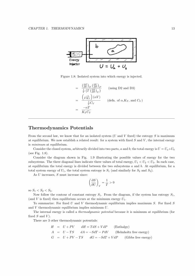
Figure 1.8: Isolated system into which energy is injected.
=
(∂P∂V
)T
(∂V∂T
)P
1T
(T(∂S∂T
)V
) (using D2 and D3)
=
(−1
VKT
)(αV )
1T CV
(defn. of α,KT , and CV )
=−αT
KTCV
Thermodynamics Potentials
From the second law, we know that for an isolated system (U and V fixed) the entropy S is maximum
at equilibrium. We now establish a related result: for a system with fixed S and V , the internal energy
is minimum at equilibrium.
Consider the closed system, arbitrarily divided into two parts, a and b; the total energy is U = Ua+Ub
(see Fig. 1.8).
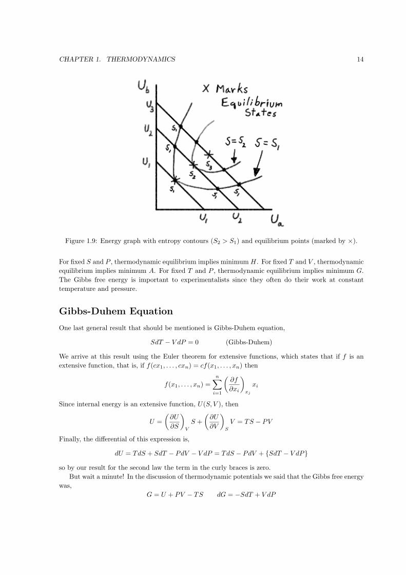
Consider the diagram shown in Fig. 1.9 illustrating the possible values of energy for the two
subsystems. The three diagonal lines indicate three values of total energy, U1 < U2 < U3. In each case,
at equilibrium the total energy is divided between the two subsystems a and b. At equilibrium, for a
total system energy of U1, the total system entropy is S1 (and similarly for S2 and S3).
As U increases, S must increase since: (∂S
∂U
)V
=1
T> 0
so S1 < S2 < S3.
Now follow the contour of constant entropy S1. From the diagram, if the system has entropy S1,
(and V is fixed) then equilibrium occurs at the minimum energy U1.
To summarize: For fixed U and V thermodynamic equilibrium implies maximum S. For fixed S
and V thermodynamic equilibrium implies minimum U .
The internal energy is called a thermodynamic potential because it is minimum at equilibrium (for
fixed S and V ).
There are 3 other thermodynamic potentials:
H = U + PV dH = TdS + V dP (Enthalpy)
A = U − TS dA = −SdT − PdV (Helmholtz free energy)
G = U + PV − TS dG = −SdT + V dP (Gibbs free energy)
CHAPTER 1. THERMODYNAMICS 14
Figure 1.9: Energy graph with entropy contours (S2 > S1) and equilibrium points (marked by ×).
For fixed S and P , thermodynamic equilibrium implies minimumH. For fixed T and V , thermodynamic
equilibrium implies minimum A. For fixed T and P , thermodynamic equilibrium implies minimum G.
The Gibbs free energy is important to experimentalists since they often do their work at constant
temperature and pressure.
Gibbs-Duhem Equation
One last general result that should be mentioned is Gibbs-Duhem equation,
SdT − V dP = 0 (Gibbs-Duhem)
We arrive at this result using the Euler theorem for extensive functions, which states that if f is an
extensive function, that is, if f(cx1, . . . , cxn) = cf(x1, . . . , xn) then
f(x1, . . . , xn) =
n∑i=1
(∂f
∂xi
)xj
xi
Since internal energy is an extensive function, U(S, V ), then
U =
(∂U
∂S
)V
S +
(∂U
∂V
)S
V = TS − PV
Finally, the differential of this expression is,
dU = TdS + SdT − PdV − V dP = TdS − PdV + SdT − V dP
so by our result for the second law the term in the curly braces is zero.
But wait a minute! In the discussion of thermodynamic potentials we said that the Gibbs free energy
was,
G = U + PV − TS dG = −SdT + V dP

CHAPTER 1. THERMODYNAMICS 15
Does the Gibbs-Duhem equation imply that dG = 0? No, because we’ve been neglecting the dependance
of the energy on number of particles; instead of writing U(S, V ) it’s more complete to write U(S, V,N).
The second law is then generalized to,
dU = TdS − PdV + µdN
where µ is the chemical potential. The full form of the Gibbs-Duhem equation is then
SdT − V dP +Ndµ = 0 (Gibbs-Duhem)
so dG = Ndµ, that is the Gibbs free energy is also the chemical potential per particle.
Van der Waals Equation of State (Pathria §12.2)Real substances have complicated equations of state. Van der Waals introduced a simple model that
extends the ideal gas law to dense gases and liquids.
The Van der Waals equation of state is:(P +
an2
V 2
)(V − bn) = nRT
where n is the number of moles and the positive constants a and b depend on the material. To understand
the origin of these constants, let’s consider them separately.
Take a = 0, then:
P =nRT
(V − bn)
Notice that P → ∞ if V → bn. There is a minimum volume to which we can compress the gas; for
one mole, this volume is b so b/NA is the volume of a single molecule. This term simulates the strong
repulsion between atoms when they are brought close together (Coulomb repulsion of electron shells).
To understand the other constant, a, write the equation of state as,
P =nRT
V − nb− an2
V 2
The larger the value of a, the smaller the pressure. This term represents the weak, attractive force
between atoms in the gas. This binding force reduces the pressure required to contain the gas in
a volume V . The smaller the volume, the closer the atoms get and the stronger this binding force
becomes. However, if we further decrease V , the repulsive term, (V − nb), kicks in and keeps the gas
from collapsing.
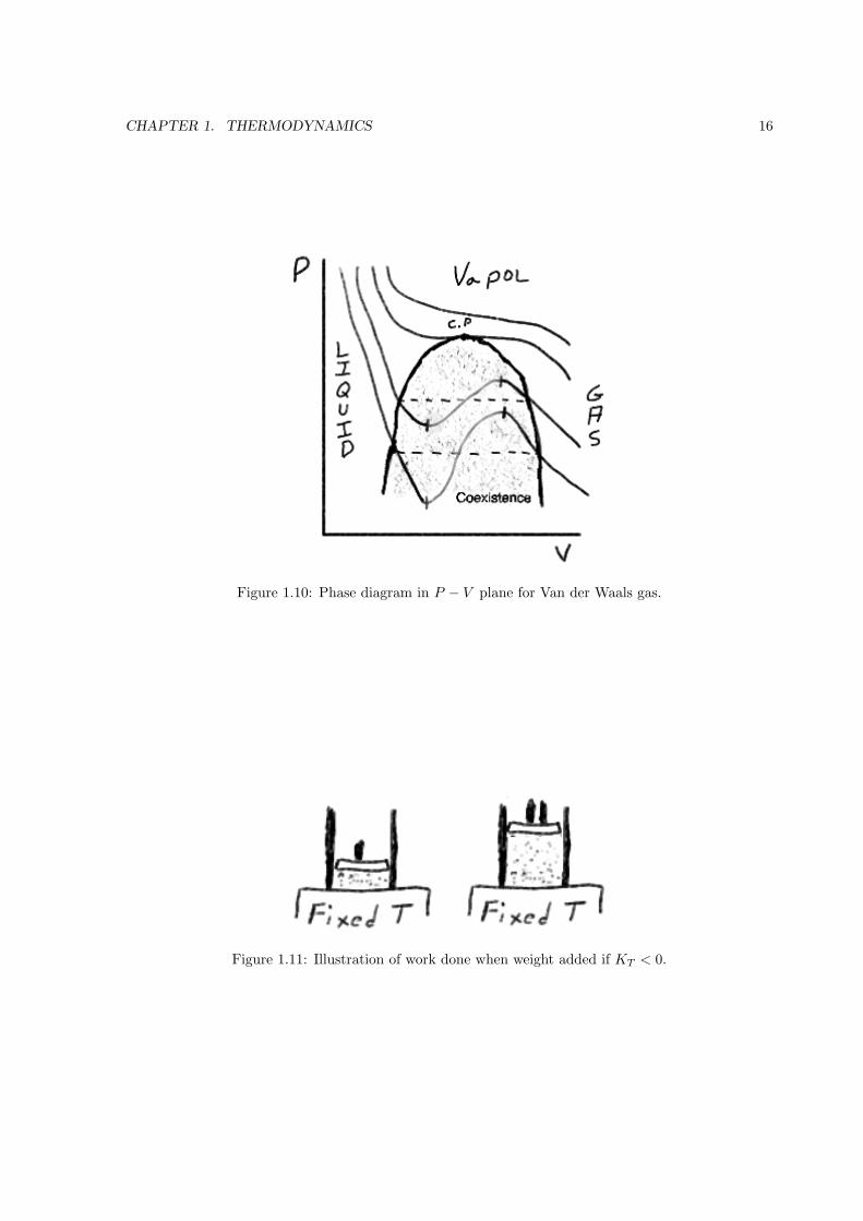
Fig. 1.10 shows the isotherms on the P −V diagram. The inflection point is called the critical point.
Using the fact that (∂P/∂V )T = (∂2P/∂V 2)T = 0 at the critical point you can work out the critical
values,
Tc =8a
27bRPc =
a
27b2Vc = 3bn
PcVc
nRTc=
3
8
For T < Tc the equation of state has an S-shape.
The region where the slope (∂P/∂V )T is positive is thermodynamically impossible; this region is
called the spinoidal region. The isothermal compressibility
KT ≡ − 1
V
(∂V
∂P
)T
of a substance must be positive or else second law is violated. To understand why, consider Fig. 1.11;
weight is added to the piston and if KT < 0 then the piston rises. Heat energy is spontaneously removed
from the reservoir and converted into work, a violation of the second law of thermodynamics.
CHAPTER 1. THERMODYNAMICS 16
Figure 1.10: Phase diagram in P − V plane for Van der Waals gas.
Figure 1.11: Illustration of work done when weight added if KT < 0.

CHAPTER 1. THERMODYNAMICS 17
Figure 1.12: Phase diagram in P − T plane.
Figure 1.13: Phase diagram in P − V plane.
Thermodynamics of Phase Transitions
The equation of state for a real substance is a complicated function, especially since we have phase
transitions. Since the EOS is difficult to draw in 3D, we often look at 2D projections (see Fig. 1.12 and
1.13).
What makes the van der Waals model so interesting is that the critical point in the model is liquid-gas
critical point, the point with the highest temperature at which liquid and gas can coexist.
Given that the spinoidal bend in the van der Waals equation of state is forbidden, you should be
curious as to what replaces it. Specifically, if we travel along an isotherm by increasing the pressure to
take the system from the gas phase (large V ) to the liquid phase (small V ), what does this isotherm
look like?
To answer this question, consider the Gibbs free energy,
dG = −SdT + V dP
Say that starting from PA, we move along the isotherm of temperature T0 < Tc. Along an isotherm
dT = 0 so
G(P, T0) =
∫ P
PA
V dP + C
where the constant of integration C can be a function of T0 and PA.
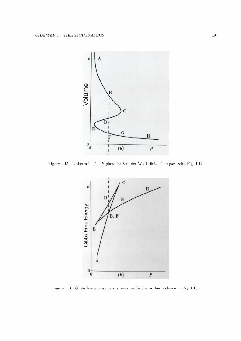
By rotating the P − V diagram to a V − P diagram (see Fig. 1.15, the qualitative shape of the
integral∫V dP can be sketched to give the Gibbs free energy shown in Fig. 1.16. Finally, the Gibbs
free energy is a thermodynamic potential that is minimum at equilibrium for fixed P and T . This
means that in traveling from point A to point H the pressure at points B through F must be equal.
CHAPTER 1. THERMODYNAMICS 18
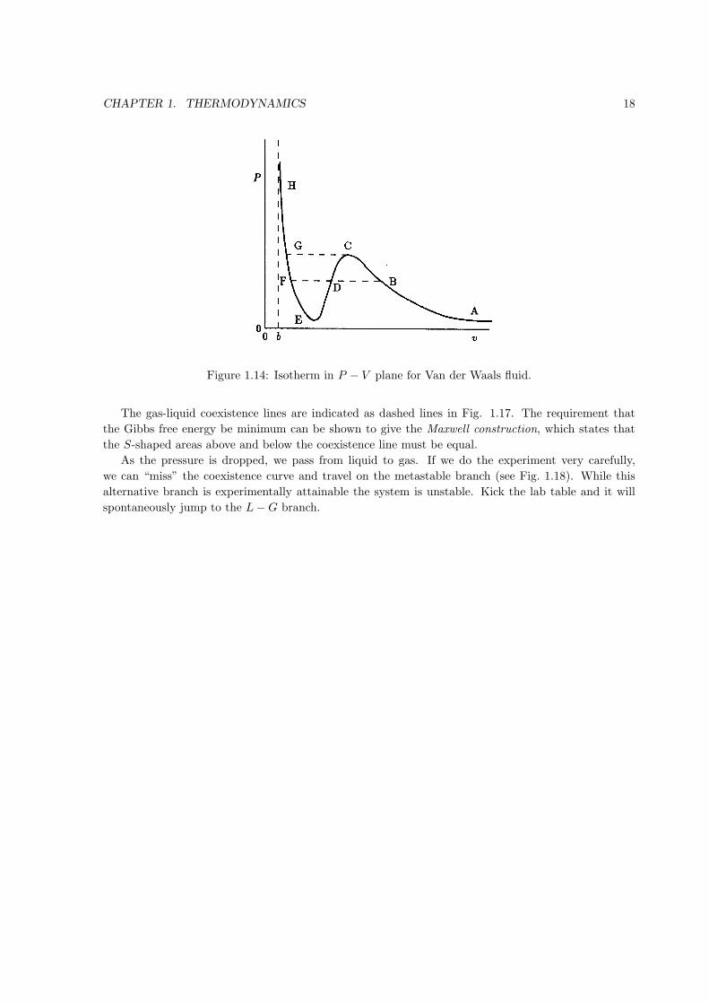
Figure 1.14: Isotherm in P − V plane for Van der Waals fluid.
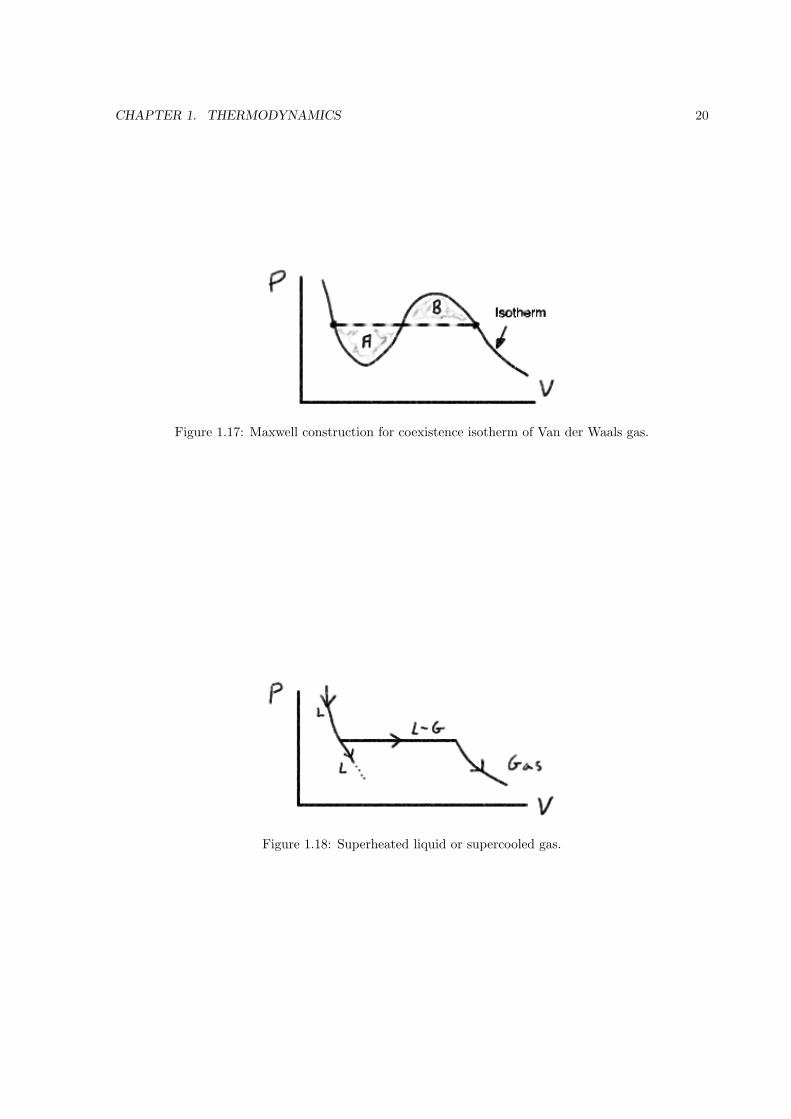
The gas-liquid coexistence lines are indicated as dashed lines in Fig. 1.17. The requirement that
the Gibbs free energy be minimum can be shown to give the Maxwell construction, which states that
the S-shaped areas above and below the coexistence line must be equal.
As the pressure is dropped, we pass from liquid to gas. If we do the experiment very carefully,
we can “miss” the coexistence curve and travel on the metastable branch (see Fig. 1.18). While this
alternative branch is experimentally attainable the system is unstable. Kick the lab table and it will
spontaneously jump to the L−G branch.
CHAPTER 1. THERMODYNAMICS 19
Vo
lum
e
Figure 1.15: Isotherm in V − P plane for Van der Waals fluid. Compare with Fig. 1.14
Gib
bs F
ree
En
erg
y
Figure 1.16: Gibbs free energy versus pressure for the isotherm shown in Fig. 1.15.
CHAPTER 1. THERMODYNAMICS 20
Figure 1.17: Maxwell construction for coexistence isotherm of Van der Waals gas.
Figure 1.18: Superheated liquid or supercooled gas.
Chapter 2
Ensemble Theory I
Ergodic Hypothesis (§2.1 – 2.2)Lecture 4
Since this is a statistical mechanics class, it is time that we end our brief review of thermodynamics
and move on to statistical mechanics. Pathria and Beale give an introduction to ensemble theory in
their Chapter 1 then give a more formal exposition in Chapter 2. In these notes the coverage is slightly
different, just to give you an alternative way to understand how it all fits together.
Given certain information about a substance (e.g., equation of state, heat capacity), thermodynamics
allows us to derive various other quantities. What is missing is a way to bridge from the mechanical
(classical or quantum) description of atomic interactions to the macroscopic level of thermodynamics.
Statistical mechanics serves as the bridge.
We first consider the formulation of statistical mechanics using classical mechanics. Since Gibbs,
Maxwell, and Boltzmann established the theory with no knowledge of quantum physics we retrace their
steps. Some systems (e.g., dilute gas) are well described by classical mechanics. Surprisingly we later
find that the quantum systems are not much harder to do. In fact Pathria and Beale start with quantum
systems, where states are easier to count, and then formulate ensemble theory for classical system in
their Chapter 2.
From Hamiltonian dynamics, we know that a system is completely described by its canonical coor-
dinates and momenta. For an N -particle system, we write the coordinates q1, q2, ..., q3N (in 3D each
particle has 3 coordinates, such as x, y, and z). Similarly the momenta are p1, p2, ..., p3N .
The instantaneous state of the system is given by:
(q, p) ≡ (q1, ..., q3N , p1,..., p3N )
The system is not frozen in this state; particles move and interact and thus the q’s and p’s change with
time. The Hamiltonian may be used to compute the dynamics.
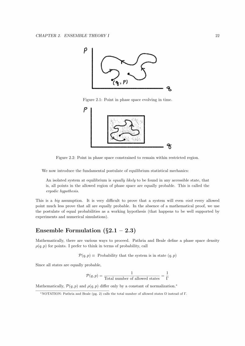
At any instant in time, the values (q, p) may be viewed as a point in 6N dimensional space (hard
to draw). In time, this point moves around in this phase space, the trajectory completely describes the
evolution of the system (see Fig. 2.1).
It is neither possible nor desirable to compute this trajectory for real systems (in which N ≈ 1023).
The trajectory cannot wander arbitrarily through phase space. For example, if our system is isolated
(so U and V are fixed) then only points that satisfy these constraints can be reached.
In Fig. 2.2 suppose that only points within the shaded region are permitted by the constraints on
the system.
21
CHAPTER 2. ENSEMBLE THEORY I 22
Figure 2.1: Point in phase space evolving in time.
Figure 2.2: Point in phase space constrained to remain within restricted region.
We now introduce the fundamental postulate of equilibrium statistical mechanics:
An isolated system at equilibrium is equally likely to be found in any accessible state, that
is, all points in the allowed region of phase space are equally probable. This is called the
ergodic hypothesis.
This is a big assumption. It is very difficult to prove that a system will even visit every allowed
point much less prove that all are equally probable. In the absence of a mathematical proof, we use
the postulate of equal probabilities as a working hypothesis (that happens to be well supported by
experiments and numerical simulations).
Ensemble Formulation (§2.1 – 2.3)
Mathematically, there are various ways to proceed. Pathria and Beale define a phase space density
ρ(q, p) for points. I prefer to think in terms of probability, call
P(q, p) ≡ Probability that the system is in state (q, p)
Since all states are equally probable,
P(q, p) =1
Total number of allowed states=
1
Γ
Mathematically, P(q, p) and ρ(q, p) differ only by a constant of normalization.∗
∗NOTATION: Pathria and Beale (pg. 2) calls the total number of allowed states Ω instead of Γ.
CHAPTER 2. ENSEMBLE THEORY I 23
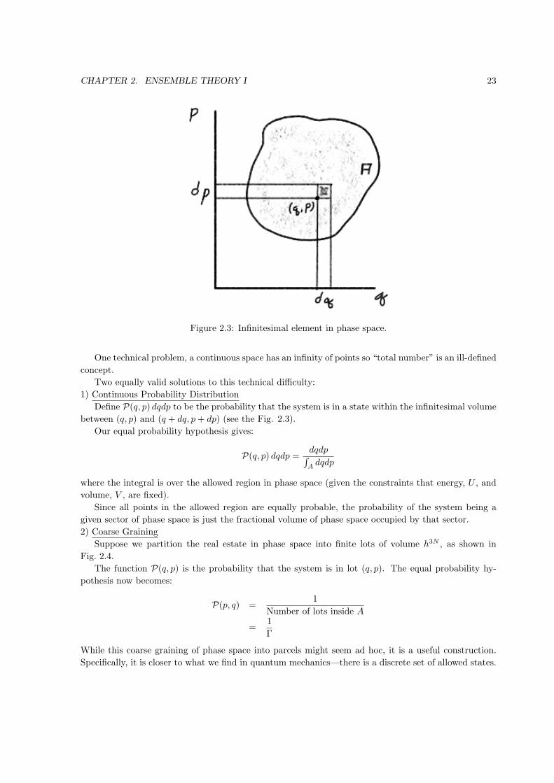
Figure 2.3: Infinitesimal element in phase space.
One technical problem, a continuous space has an infinity of points so “total number” is an ill-defined
concept.
Two equally valid solutions to this technical difficulty:
1) Continuous Probability Distribution
Define P(q, p) dqdp to be the probability that the system is in a state within the infinitesimal volume
between (q, p) and (q + dq, p+ dp) (see the Fig. 2.3).
Our equal probability hypothesis gives:
P(q, p) dqdp =dqdp∫Adqdp
where the integral is over the allowed region in phase space (given the constraints that energy, U , and
volume, V , are fixed).
Since all points in the allowed region are equally probable, the probability of the system being a
given sector of phase space is just the fractional volume of phase space occupied by that sector.
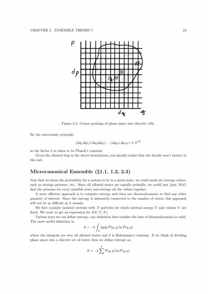
2) Coarse Graining
Suppose we partition the real estate in phase space into finite lots of volume h3N , as shown in
Fig. 2.4.
The function P(q, p) is the probability that the system is in lot (q, p). The equal probability hy-
pothesis now becomes:
P(p, q) =1
Number of lots inside A
=1
Γ
While this coarse graining of phase space into parcels might seem ad hoc, it is a useful construction.
Specifically, it is closer to what we find in quantum mechanics—there is a discrete set of allowed states.
CHAPTER 2. ENSEMBLE THEORY I 24
Figure 2.4: Coarse graining of phase space into discrete cells.
By the uncertainty principle:
(∆q1∆p1)(∆q2∆p2) . . . (∆q3N∆p3N ) ≈ h3N
so the factor h is taken to be Planck’s constant.
Given the allowed slop in the above formulation, you should realize that the details won’t matter in
the end.
Microcanonical Ensemble (§1.1, 1.2, 2.3)Now that we know the probability for a system to be in a given state, we could work out average values,
such as average pressure, etc.. Since all allowed states are equally probable, we could just (just, HA!)
find the pressure for every possible state and average all the values together.
A more efficient approach is to compute entropy and then use thermodynamics to find any other
quantity of interest. Since the entropy is intimately connected to the number of states, this approach
will not be as difficult as it sounds.
We first consider isolated systems with N particles for which internal energy U and volume V are
fixed. We want to get an expression for S(U, V,N).
Various ways we can define entropy; any definition that satisfies the laws of thermodynamics is valid.
The most useful definition is,
S = −k
∫A
dqdpP(q, p) lnP(q, p)
where the integrals are over all allowed states and k is Boltzmann’s constant. If we think of dividing
phase space into a discrete set of states then we define entropy as,
S = −kΓ∑
P(q, p) lnP(q, p)
CHAPTER 2. ENSEMBLE THEORY I 25
Probability theory tells us this expression for S gives the uncertainty (or disorder) in a system. You
can prove that it possesses all the desired features for entropy, for example, it is maximum when all
states are equally probable thus S is maximum at equilibrium.
Example: Suppose that a system has only 2 states, a and b. Show that the entropy is maximum
when Pa = Pb = 1/2.
Solution: Our definition for entropy is:
S = −kΓ∑
P lnP= −k(Pa lnPa + Pb lnPb)
But probabilities must sum to one so Pa + Pb = 1 or Pb = 1− Pa so:
S = −k(Pa lnPa + (1− Pa) ln(1−Pa))
To find the maximum, we take the derivative
∂S
∂Pa= −k
(lnPa + Pa
(1
Pa
)− ln (1− Pa) + (1− Pa)
(−1
1−Pa
))so
0 = −k(lnPa − ln(1− Pa))
or
Pa = 1−Pa
so Pa = 1/2. You can check that this extremum is a maximum.
For an isolated system, the equal probability hypothesis gives the probability P(q, p) = 1/Γ so:
S = −kΓ∑
P(q, p) lnP(q, p)
= −kΓ∑(
1
Γ
)ln
(1
Γ
)= +k
(1
Γ
)ln (Γ)
(Γ∑
1
)
= k
(1
Γ
)ln (Γ) (Γ)
= k ln Γ
Aside from the constant k, the entropy is the logarithm of the number of accessible states.
Entropy and Thermodynamics (§1.3, 2.3)We just discussed how, for a system with internal energy, U , and volume, V , the equal probability
hypothesis gave us an entropy
S = k ln Γ
CHAPTER 2. ENSEMBLE THEORY I 26
where Γ is the number of states that the system can be in. The set of allowed states for fixed U and V
is called the microcanonical ensemble.
Pathria and Beale point out that it doesn’t matter if we use
Number of states such that
U = E
U ≤ E ≤ U +∆U
E ≤ U
where E is the energy of an individual state. That is, we can count just states that have exactly energy
U , or count all states with energy in the range U and U +∆U or even counting all states with energy
less than or equal to U . This will be useful because sometimes one set of states is easier to count that
another, as you will see in later examples.
Given the number of states in the microcanonical ensemble Γ(U, V ) we have the following recipe:
1) Evaluate S(U, V ) = k ln Γ(U, V )
2) Given S(U, V ) solve for U(S, V )
3) Evaluate
T =(
∂∂S
)VU(S, V )
P = −(
∂∂V
)SU(S, V )
The third step comes from using
dU = TdS − PdV =
(∂U
∂S
)V
dS +
(∂U
∂V
)S
dV
Finally, use conventional thermodynamics to find any other desired quantities (e.g., heat capacity,
compressibility).
Notice that temperature now has a mechanical definition since
1
T=
(∂S
∂U
)V
=
(∂
∂U
)V
(k ln Γ(U, V ))
so1
T= k
1
Γ
(∂Γ
∂U
)V
or
T =1
k
Γ(U, V )(∂Γ∂U
)V
The temperature is inversely proportional to the rate at which the number of states increases as internal
energy increases. Of course it is difficult find a “number of allowed states” meter in the lab. Simpler to
calibrate thermometers that use properties, such as electrical conductivity, that vary with temperature
and are easy to measure mechanically.
For most physical systems, the number of accessible states increases as energy increases so (∂Γ/∂U) >
0. There are exceptional systems for which the energy that can be added to the system has some max-
imum saturation value. For these systems, one can have (∂Γ/∂U) < 0 giving negative temperatures.
Note that negative temperatures occur not when a system has very little energy but rather when it has
so much energy that it is running out of available states. You’ll do an example of such a system as a
homework problem.
CHAPTER 2. ENSEMBLE THEORY I 27
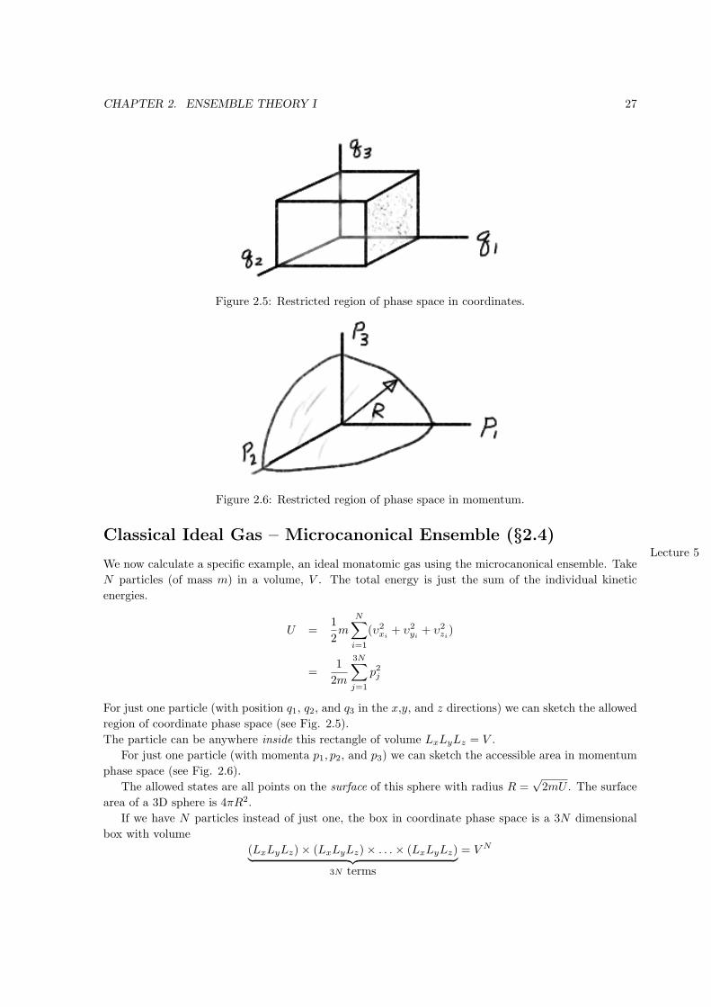
Figure 2.5: Restricted region of phase space in coordinates.
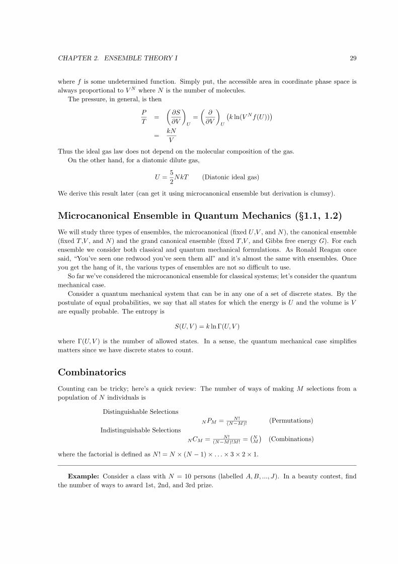
Figure 2.6: Restricted region of phase space in momentum.
Classical Ideal Gas – Microcanonical Ensemble (§2.4)Lecture 5
We now calculate a specific example, an ideal monatomic gas using the microcanonical ensemble. Take
N particles (of mass m) in a volume, V . The total energy is just the sum of the individual kinetic
energies.
U =1
2m
N∑i=1
(υ2xi
+ υ2yi+ υ2
zi)
=1
2m
3N∑j=1
p2j
For just one particle (with position q1, q2, and q3 in the x,y, and z directions) we can sketch the allowed
region of coordinate phase space (see Fig. 2.5).
The particle can be anywhere inside this rectangle of volume LxLyLz = V .
For just one particle (with momenta p1, p2, and p3) we can sketch the accessible area in momentum
phase space (see Fig. 2.6).
The allowed states are all points on the surface of this sphere with radius R =√2mU . The surface
area of a 3D sphere is 4πR2.
If we have N particles instead of just one, the box in coordinate phase space is a 3N dimensional
box with volume
(LxLyLz)× (LxLyLz)× . . .× (LxLyLz)︸ ︷︷ ︸3N terms
= V N

CHAPTER 2. ENSEMBLE THEORY I 28
Similarly, for N particles instead of one, the accessible states in momentum space are the points on the
surface of a 3N dimensional sphere. The surface area of a 3N dimensional sphere is BNR3N−1 where
BN is a geometric constant (see Appendix C in Pathria and Beale). The number of accessible states is
thus,
BNR3N−1 = BN
(√2mU
)3N−1
≈ BN (2mU)3N/2
Since N ≫ 1, we can set 3N − 1 ≈ 3N .
Collecting the above results, the total number of accessible states is the product of the number of
states in coordinate space times the number of states in momentum space, so
Γ(U, V ) =(V N)×(BN (2mU)3N/2
)= BN (V (2mU)3/2)N
We now follow the steps in our recipe; first get the entropy,
S = k ln Γ(U, V )
= kN ln(V (2mU)3/2) + k lnBN
The temperature in an ideal gas is found by solving
1
T=
(∂S
∂U
)V
= kN1
V (2mU)3/23
2V (2m)3/2U1/2
=32kN
U
This relation between energy and temperature is usually written as
U =3
2kNT (Monatomic ideal gas)
This confirms the result found in the Joule free expansion experiment—the internal energy depends
only on the temperature and not on volume.
To get the pressure we could use P = −(∂U∂V
)S. Instead let’s use
P
T=
(∂S
∂V
)U
=
(∂
∂V
)U
[kN ln(V (2mU)3/2) + k lnBN
]= kN
1
V (2mU)3/2(2mU)
3/2
=kN
V
or PV = NkT , the ideal gas law.
Our derivation was for a monatomic dilute gas such as helium or argon. Most dilute gases are not
monatomic, for example nitrogen and oxygen form diatomic molecules.
However, for dilute gases, the energy of the molecules is independent of the molecules’ positions.
This means that, in general, for a gas,
Γ(U, V ) = V Nf(U)
CHAPTER 2. ENSEMBLE THEORY I 29
where f is some undetermined function. Simply put, the accessible area in coordinate phase space is
always proportional to V N where N is the number of molecules.
The pressure, in general, is then
P
T=
(∂S
∂V
)U
=
(∂
∂V
)U
(k ln(V Nf(U))
)=
kN
V
Thus the ideal gas law does not depend on the molecular composition of the gas.
On the other hand, for a diatomic dilute gas,
U =5
2NkT (Diatonic ideal gas)
We derive this result later (can get it using microcanonical ensemble but derivation is clumsy).
Microcanonical Ensemble in Quantum Mechanics (§1.1, 1.2)We will study three types of ensembles, the microcanonical (fixed U ,V , and N), the canonical ensemble
(fixed T ,V , and N) and the grand canonical ensemble (fixed T ,V , and Gibbs free energy G). For each
ensemble we consider both classical and quantum mechanical formulations. As Ronald Reagan once
said, “You’ve seen one redwood you’ve seen them all” and it’s almost the same with ensembles. Once
you get the hang of it, the various types of ensembles are not so difficult to use.
So far we’ve considered the microcanonical ensemble for classical systems; let’s consider the quantum
mechanical case.
Consider a quantum mechanical system that can be in any one of a set of discrete states. By the
postulate of equal probabilities, we say that all states for which the energy is U and the volume is V
are equally probable. The entropy is
S(U, V ) = k ln Γ(U, V )
where Γ(U, V ) is the number of allowed states. In a sense, the quantum mechanical case simplifies
matters since we have discrete states to count.
Combinatorics
Counting can be tricky; here’s a quick review: The number of ways of making M selections from a
population of N individuals is
Distinguishable Selections
NPM = N !(N−M)! (Permutations)
Indistinguishable Selections
NCM = N !(N−M)!M ! =
(NM
)(Combinations)
where the factorial is defined as N ! = N × (N − 1)× . . .× 3× 2× 1.
Example: Consider a class with N = 10 persons (labelled A,B, ..., J). In a beauty contest, find
the number of ways to award 1st, 2nd, and 3rd prize.
CHAPTER 2. ENSEMBLE THEORY I 30
Solution: Since the selections are distinguishable (1st prize is different from 2nd prize) making the
list of possible selections we have,ABC
ACB
ABD...
The number of permutations is
10!
(10− 3)!=
10!
7!= 10 · 9 · 8 = 720
Example (cont.): If in a class of 10 students three students flunk the class, find the number of ways
of selecting them.
Solution: In this case the selections are indistinguishable so the list of possible selections is
ABC
ABD...
The number of combinations is 10!7!3! = 120.
Finally, the number of ways of putting M indistinguishable objects into N distinguishable boxes is(N +M − 1
M
)=
(N +M − 1
N − 1
)=
(N +M − 1)!
(N − 1)!M !
Quantum Harmonic Oscillators (§3.8)Lecture 6
Our first quantum mechanics example is a system composed of a collection of N uncoupled harmonic
oscillators. The total energy U is fixed; this system has no volume (or pressure) so the number of states
Γ only depends on U . The oscillators are distinguishable.
The energy levels for an individual oscillator are ϵ(n) = hω(n + 1/2), n = 0, 1, 2, .... Call ni the
energy level for oscillator i and
M =N∑i=1
ni
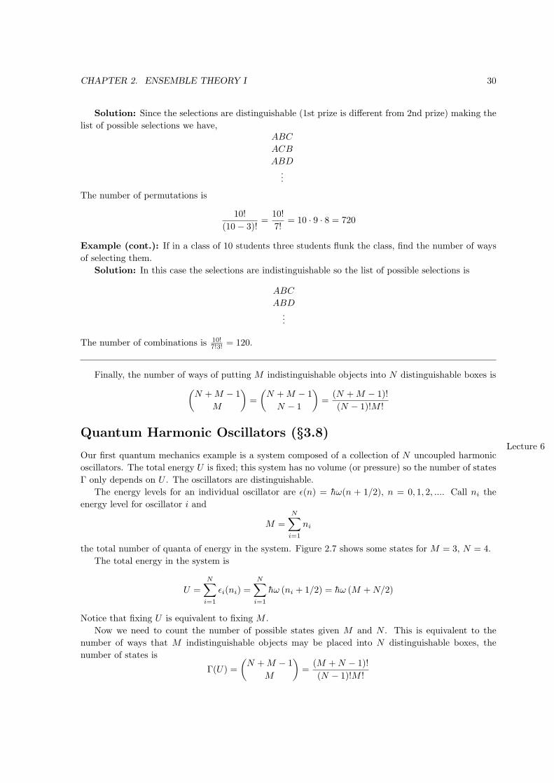
the total number of quanta of energy in the system. Figure 2.7 shows some states for M = 3, N = 4.
The total energy in the system is
U =N∑i=1
ϵi(ni) =N∑i=1
hω (ni + 1/2) = hω (M +N/2)
Notice that fixing U is equivalent to fixing M .
Now we need to count the number of possible states given M and N . This is equivalent to the
number of ways that M indistinguishable objects may be placed into N distinguishable boxes, the
number of states is
Γ(U) =
(N +M − 1
M
)=
(M +N − 1)!
(N − 1)!M !

CHAPTER 2. ENSEMBLE THEORY I 31
Figure 2.7: Two possible quantum harmonic oscillator system states for M = 3, N = 4.
where M = U/hω −N/2.
The entropy in the system is
S(U) = k ln Γ ≈ k [(M +N) ln (M +N)−M lnM −N lnN ]
where we’ve used the approximation ln(x!) ≈ x ln(x) − x for x ≫ 1. We can now proceed to compute
other thermodynamic quantities. For example,
1
T=
dS
dU=
dS
dM
dM
dU= (k ln(M +N)− k lnM)
(1
hω
)which gives us the following relation between M and T ,
M =N
ehω/kT − 1
so
U =hωN
ehω/kT − 1+
1
2hωN
Notice that M → 0, U → 12 hωN as T → 0 and M → ∞, U → ∞ as T → ∞. This is the Einstein model
for a solid. Though it gives the right qualitative behavior and is better than a classical description of
a solid this model is superseded by the Debye model.
Example: Find the heat capacity for a system of N quantum mechanical harmonic oscillators.
Solution: Since the system cannot do mechanical work, CP = CV = C. In other words, the internal
energy is only a function of temperature so,
C =dU
dT=
dU
dM
dM
dT
= (hω)−N(
ehω/kT − 1)2 −hω
kT 2
=
(hω
kT
)2kN(
ehω/kT − 1)2
CHAPTER 2. ENSEMBLE THEORY I 32
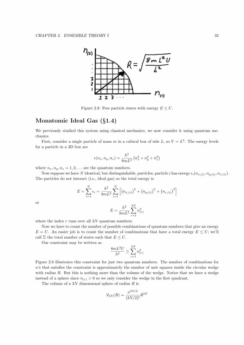
Figure 2.8: Free particle states with energy E ≤ U .
Monatomic Ideal Gas (§1.4)We previously studied this system using classical mechanics, we now consider it using quantum me-
chanics.
First, consider a single particle of mass m in a cubical box of side L, so V = L3. The energy levels
for a particle in a 3D box are
ϵ(nx, ny, nz) =h2
8mL2
(n2x + n2
y + n2z
)where nx, ny, nz = 1, 2, . . . are the quantum numbers.
Now suppose we haveN identical, but distinguishable, particles; particle i has energy ϵi(nx,(i), ny,(i), nz,(i)).
The particles do not interact (i.e., ideal gas) so the total energy is
E =N∑i=1
ϵi =h2
8mL2
N∑i=1
[(nx,(i)
)2+(ny,(i)
)2+(nz,(i)
)2]or
E =h2
8mL2
3N∑r=1
n2(r)
where the index r runs over all 3N quantum numbers.
Now we have to count the number of possible combinations of quantum numbers that give an energy
E = U . An easier job is to count the number of combinations that have a total energy E ≤ U ; we’ll
call Σ the total number of states such that E ≤ U .
Our constraint may be written as
8mL2U
h2≥
3N∑r=1
n2(r)
Figure 2.8 illustrates this constraint for just two quantum numbers. The number of combinations for
n’s that satisfies the constraint is approximately the number of unit squares inside the circular wedge
with radius R. But this is nothing more than the volume of the wedge. Notice that we have a wedge
instead of a sphere since n(r) > 0 so we only consider the wedge in the first quadrant.
The volume of a 3N dimensional sphere of radius R is
V3N (R) =π3N/2
(3N/2)!R3N
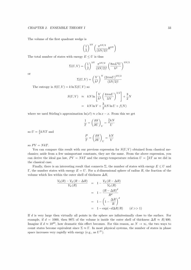
CHAPTER 2. ENSEMBLE THEORY I 33
The volume of the first quadrant wedge is(1
2
)3N (π3N/2
(3N/2)!R3N
)The total number of states with energy E ≤ U is thus
Σ(U, V ) =
(1
2
)3Nπ3N/2
(3N/2)!
(8mL2U
h2
)3N/2
or
Σ(U, V ) =
(V
h3
)N(2πmU)
3N/2
(3N/2)!
The entropy is S(U, V ) = k lnΣ(U, V ) so
S(U, V ) ≈ kN ln
[V
h3
(4πmU
3N
)3/2]+
3
2N
= kN lnV +3
2kN lnU + f(N)
where we used Stirling’s approximation ln(x!) ≈ x lnx− x. From this we get
1
T=
(∂S
∂U
)V
=32kN
U
so U = 32kNT and
P
T=
(∂S
∂V
)U
=kN
V
so PV = NkT .
You can compare this result with our previous expression for S(U, V ) obtained from classical me-
chanics; aside from a few unimportant constants, they are the same. From the above expression, you
can derive the ideal gas law, PV = NkT and the energy-temperature relation U = 32kT as we did in
the classical case.
Finally, there is an interesting result that connects Σ, the number of states with energy E ≤ U and
Γ, the number states with energy E = U . For a d-dimensional sphere of radius R, the fraction of the
volume which lies within the outer shell of thickness ∆R,
Vd(R)− Vd (R−∆R)
Vd (R)= 1− Vd (R−∆R)
Vd (R)
= 1− (R−∆R)d
Rd
= 1−(1− ∆R
R
)d
= 1− exp(−d∆R/R) (d >> 1)
If d is very large then virtually all points in the sphere are infinitesimally close to the surface. For
example, if d = 1000, then 90% of the volume is inside the outer shell of thickness ∆R ≈ R/400.
Imagine if d ≈ 1023, how dramatic this effect becomes. For this reason, as N → ∞, the two ways to
count states become equivalent since Σ ≈ Γ. In most physical systems, the number of states in phase
space increases very rapidly with energy (e.g., as UN ).
CHAPTER 2. ENSEMBLE THEORY I 34
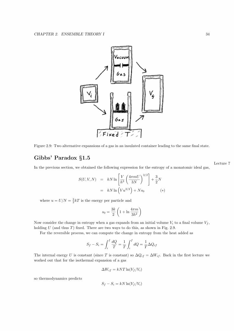
Figure 2.9: Two alternative expansions of a gas in an insulated container leading to the same final state.
Gibbs’ Paradox §1.5Lecture 7
In the previous section, we obtained the following expression for the entropy of a monatomic ideal gas,
S(U, V,N) = kN ln
[V
h3
(4πmU
3N
)3/2]+
3
2N
= kN ln(V u3/2
)+Ns0 (∗)
where u = U/N = 32kT is the energy per particle and
s0 =3k
2
(1 + ln
4πm
3h2
)Now consider the change in entropy when a gas expands from an initial volume Vi to a final volume Vf ,
holding U (and thus T ) fixed. There are two ways to do this, as shown in Fig. 2.9.
For the reversible process, we can compute the change in entropy from the heat added as
Sf − Si =
∫ f
i
dQ
T=
1
T
∫ f
i
dQ =1
T∆Qif
The internal energy U is constant (since T is constant) so ∆Qif = ∆Wif . Back in the first lecture we
worked out that for the isothermal expansion of a gas
∆Wif = kNT ln(Vf/Vi)
so thermodynamics predicts
Sf − Si = kN ln(Vf/Vi)
CHAPTER 2. ENSEMBLE THEORY I 35
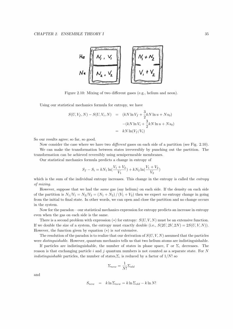
Figure 2.10: Mixing of two different gases (e.g., helium and neon).
Using our statistical mechanics formula for entropy, we have
S(U, Vf , N)− S(U, Vi, N) = (kN lnVf +3
2kN lnu+Ns0)
−(kN lnVi +3
2kN lnu+Ns0)
= kN ln(Vf/Vi)
So our results agree; so far, so good.
Now consider the case where we have two different gases on each side of a partition (see Fig. 2.10).
We can make the transformation between states irreversibly by punching out the partition. The
transformation can be achieved reversibly using semipermeable membranes.
Our statistical mechanics formula predicts a change in entropy of
Sf − Si = kN1 ln(V1 + V2
V1) + kN2 ln(
V1 + V2
V2)
which is the sum of the individual entropy increases. This change in the entropy is called the entropy
of mixing.
However, suppose that we had the same gas (say helium) on each side. If the density on each side
of the partition is N1/V1 = N2/V2 = (N1 +N2) / (V1 + V2) then we expect no entropy change in going
from the initial to final state. In other words, we can open and close the partition and no change occurs
in the system.
Now for the paradox—our statistical mechanics expression for entropy predicts an increase in entropy
even when the gas on each side is the same.
There is a second problem with expression (∗) for entropy: S(U, V,N) must be an extensive function.
If we double the size of a system, the entropy must exactly double (i.e., S(2U, 2V, 2N) = 2S(U, V,N)).
However, the function given by equation (∗) is not extensive.The resolution of the paradox is to realize that our derivation of S(U, V,N) assumed that the particles
were distinguishable. However, quantum mechanics tells us that two helium atoms are indistinguishable.
If particles are indistinguishable, the number of states in phase space, Γ or Σ, decreases. The
reason is that exchanging particle i and j quantum numbers is not counted as a separate state. For N
indistinguishable particles, the number of states,Σ, is reduced by a factor of 1/N ! so
Σnew =1
N !Σold
and
Snew = k lnΣnew = k lnΣold − k lnN !
CHAPTER 2. ENSEMBLE THEORY I 36
= Sold − k lnN !
= Sold − k (N lnN −N)
= kN ln
(V
N
(U
N
)3/2)
+NC
where C is a constant. You can see that S(U, V,N)new is an extensive function so this resolves Gibbs’
paradox. This corrected expression for the entropy of a monatomic ideal gas is called the Sackur-Tetrode
equation. Our previous results (before the 1/N ! correction) are unaffected because the term added to
the entropy is independent of U and V .
If instead of one type of particle we haveM distinguishable species with particle numbersN1, . . . , NM
then the Gibbs correction is
Σnew =1
N1! . . . NM !Σold
so
Snew = Sold − k lnN1!− . . .− k lnNM !
which you can check makes S(U, V,N1, . . . , NM )new an extensive function.
Finally, note that the combinatorial argument which gave us the 1/N ! factor assumes only one
particle per quantum state. This is a good assumption except at low temperatures where particle
occupancy of states has to be treated more carefully. We return to do the low temperature scenario
when we consider Fermi and Bose quantum ideal gases.

Chapter 3
Ensemble Theory II
Canonical Ensemble (§3.2)Lecture 8
Our fundamental definition for entropy is
S = −k
states∑i
Pi lnPi
where the sum is over all allowed states, and Pi is the probability of each state.
In the microcanonical ensemble, only states that had energy Ei = U were allowed and all allowed
states were equally probable, thus
Pi =1
Γ(microcanonical ensemble)
where Γ was the total number of allowed states. We found that sometimes it was more convenient to
find Σ, the number of states with energy Ei ≤ U . Besides, we saw that Γ ≈ Σ which comes from
the fact that there are very few states with energy less than U (i.e., the number of states increases
astronomically fast with increasing energy).
In the canonical ensemble, we let all states be allowed states but demand that the average energy
equal U . The average energy is
⟨E⟩ =states∑
i
EiPi
We now allow states with energy Ei > U . However, our constraint on ⟨E⟩ will assign them low
probability.
We want to determine Pi such that S is maximum. There are two constraints on Pi,∑i
Pi = 1 ;∑i
EiPi = U
The first is the demand that probabilities must sum to unity; the second is our condition that ⟨E⟩ = U .
To maximize S with these constraints, we use the method of Lagrange multipliers. Introduce the
function
W = S − α′∑i
Pi − β′∑i
EiPi
where α′ and β′ are Lagrange multipliers.
37
CHAPTER 3. ENSEMBLE THEORY II 38
We seek to maximize W so we compute ∂W/∂Pj and set the derivative to zero,
∂W
∂Pj=
∂
∂Pj
(−k∑i
Pi lnPi − α′∑i
Pi − β′∑i
EiPi
)
= −∑i
∂
∂Pj(kPi lnPi + α′Pi + β′EiPi)
= −∑i
(k lnPj + k + α′ + β′Ej) δij
= −k(lnPj + α+ βEj)
where α ≡ 1 + α′/k, β ≡ β′/k.
Setting ∂W/∂Pj = 0 gives
lnPj = −α− βEj
or
Pj = e−αe−βEj
Notice that in the canonical ensemble, states are not equally probable. Instead, the higher the energy
of a state, the lower the probability (we’ll see β > 0 so as Ej increases e−βEj decreases so Pj decreases).
But isn’t our fundamental assumption of statistical mechanics that all accessible states are equally
probable? Not quite. We stated that for an isolated system (no energy in or out), all accessible
states were equally probable. The canonical ensemble describes equilibrium systems but not isolated
equilibrium systems since energy is not fixed. So what type of equilibrium system does the canonical
ensemble describe? We’ll see in a just a few pages (look at Fig. 3.2 if you just can’t wait).
The two Lagrange multipliers are determined by imposing the constraints∑i
Pi = 1;∑
EiPi = U
on the above expression for Pj .
From the constraint that the probabilities sum to unity.∑i
(e−αe−βEi) = 1
or
e−α∑i
e−βEi = 1
We define the partition function as,
QN ≡∑i
e−βEi
so e−αQN = 1 or
α = lnQN
This gives us α in terms of β.
The probabilities are thus
Pi =e−βEi∑i
e−βEi=
e−βEi
QN

CHAPTER 3. ENSEMBLE THEORY II 39
For the constraint demanding that the average energy equal U ,
U =∑i
EiPi =∑i
Eie−βEi
QN
=1
QN
∑i
Eie−βEi
= − 1
QN
∂
∂β
∑i
e−βEi (slick trick)
= − 1
QN
∂
∂βQN
so
U = − ∂
∂βlnQN
While this is not an explicit expression for β, it turns out to be good enough. Notice the slick trick
used above to change the sum by introducing a derivative.
Collecting our results, we can write the entropy as
S = −k∑i
Pi lnPi
= −k∑i
(1
QNe−βEi
)ln
(1
QNe−βEi
)= −k
∑i
(1
QNe−βEi
)[−βEi − lnQN ]
= +kβ∑i
1
QNEie
−βEi + k lnQN
∑i
1
QNe−βEi
= kβ∑i
EiPi + k lnQN
∑i
Pi
Finally,
S = kβU + k lnQN
Our link to thermodynamics is still shaky since we haven’t nailed down β in terms of something
familiar. Let’s hammer using (∂S
∂U
)V
=1
T
then1
T=
(∂
∂U
)V
[kβU + k lnQN ] = kβ
so
β =1
kT; T =
1
kβ
which is the link we wanted to find.
Our entropy is
S =1
TU + k lnQN
or
kT lnQN = TS − U = −A
CHAPTER 3. ENSEMBLE THEORY II 40
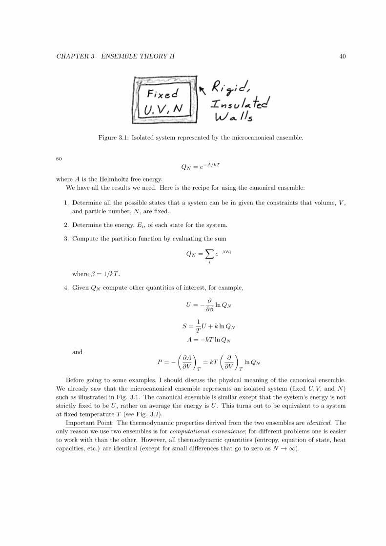
Figure 3.1: Isolated system represented by the microcanonical ensemble.
so
QN = e−A/kT
where A is the Helmholtz free energy.
We have all the results we need. Here is the recipe for using the canonical ensemble:
1. Determine all the possible states that a system can be in given the constraints that volume, V ,
and particle number, N , are fixed.
2. Determine the energy, Ei, of each state for the system.
3. Compute the partition function by evaluating the sum
QN =∑i
e−βEi
where β = 1/kT .
4. Given QN compute other quantities of interest, for example,
U = − ∂
∂βlnQN
S =1
TU + k lnQN
A = −kT lnQN
and
P = −(∂A
∂V
)T
= kT
(∂
∂V
)T
lnQN
Before going to some examples, I should discuss the physical meaning of the canonical ensemble.
We already saw that the microcanonical ensemble represents an isolated system (fixed U, V, and N)
such as illustrated in Fig. 3.1. The canonical ensemble is similar except that the system’s energy is not
strictly fixed to be U , rather on average the energy is U . This turns out to be equivalent to a system
at fixed temperature T (see Fig. 3.2).
Important Point: The thermodynamic properties derived from the two ensembles are identical. The
only reason we use two ensembles is for computational convenience; for different problems one is easier
to work with than the other. However, all thermodynamic quantities (entropy, equation of state, heat
capacities, etc.) are identical (except for small differences that go to zero as N → ∞).
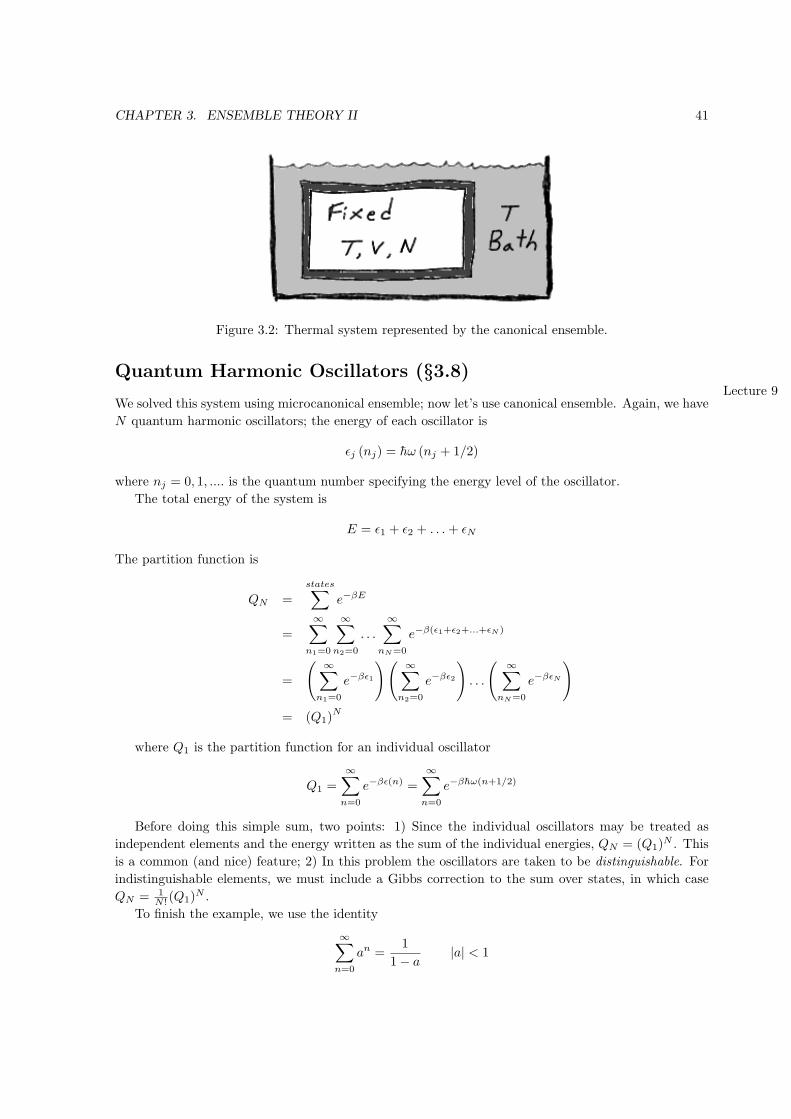
CHAPTER 3. ENSEMBLE THEORY II 41
Figure 3.2: Thermal system represented by the canonical ensemble.
Quantum Harmonic Oscillators (§3.8)Lecture 9
We solved this system using microcanonical ensemble; now let’s use canonical ensemble. Again, we have
N quantum harmonic oscillators; the energy of each oscillator is
ϵj (nj) = hω (nj + 1/2)
where nj = 0, 1, .... is the quantum number specifying the energy level of the oscillator.
The total energy of the system is
E = ϵ1 + ϵ2 + . . .+ ϵN
The partition function is
QN =states∑
e−βE
=∞∑
n1=0
∞∑n2=0
. . .∞∑
nN=0
e−β(ϵ1+ϵ2+...+ϵN )
=
( ∞∑n1=0
e−βϵ1
)( ∞∑n2=0
e−βϵ2
). . .
( ∞∑nN=0
e−βϵN
)= (Q1)
N
where Q1 is the partition function for an individual oscillator
Q1 =∞∑
n=0
e−βϵ(n) =∞∑
n=0
e−βhω(n+1/2)
Before doing this simple sum, two points: 1) Since the individual oscillators may be treated as
independent elements and the energy written as the sum of the individual energies, QN = (Q1)N . This
is a common (and nice) feature; 2) In this problem the oscillators are taken to be distinguishable. For
indistinguishable elements, we must include a Gibbs correction to the sum over states, in which case
QN = 1N ! (Q1)
N .
To finish the example, we use the identity
∞∑n=0
an =1
1− a|a| < 1
CHAPTER 3. ENSEMBLE THEORY II 42
so
Q1 =e−βhω/2
1− e−βhω=
1
2sinh (βhω/2)
Using
U = − ∂
∂βlnQN = − ∂
∂β(N lnQ1)
then
U =1
2Nhω coth(βhω/2)
You can check that this result matches our microcanonical result for U (recall β = 1/kT ).
Monatomic Ideal Gas – Canonical Ensemble
This is the third (and I promise, the last) time we derive the thermodynamics of this system using
statistical mechanics. It is worth repeating using the canonical ensemble since our derivation will be
useful when we study fermion and boson systems.
Recall that the energy levels of a particle in a cubic box of volume V = L3 are
ϵ (nx, ny, nz) =h2
8mL2(n2
x + n2y + n2
z)
Since we have an ideal gas, the interactions between the particles are negligible. The partition function
is thus
QN =1
N !QN
1
where Q1 is the partition function for a single particle. Notice we have a factor of 1/N ! out in front
because the particles are indistinguishable.
The single particle partition function is
Q1 =∞∑
nx=1
∞∑ny=1
∞∑nz=1
e−βϵ(nx,ny,nz)
or
Q1 =
( ∞∑nx=1
exp
(−πλ2n2
x
4L2
))(same for ny) (same for nz)
where
λ =h√
2πmkT
is the thermal wavelength (the de Broglie wavelength of a particle with energy ≈ kT ).
In the classical limit the de Broglie wavelength of the particles is much smaller than the distance
between them(λ ≪ 3
√V/N = L/ 3
√N), so we may replace the sums with integrals.
∞∑nx=1
exp
(−πλ2n2
x
4L2
)≈
∞∫0
dx exp
(−πλ2x2
4L2
)This Gaussian integral is easy to compute,
∞∫0
dx exp
(−πλ2x2
4L2
)=
1
2
√π(
πλ2
4L2
) =L
λ
CHAPTER 3. ENSEMBLE THEORY II 43
so
Q1 ≈(L
λ
)(L
λ
)(L
λ
)=
V
λ3
The N particle partition function is
QN =1
N !QN
1 =1
N !
(V
λ3
)N
The internal energy is
U = −(
∂
∂β
)V
lnQN = 3N
(∂
∂β
)V
lnλ =3N
2β=
3
2NkT
The pressure is
P = kT
(∂
∂V
)T
lnQN = kT
(∂
∂V
)T
lnV N =NkT
V
confirming all of our previous results.
Canonical Ensemble in Classical Mechanics (§3.5)Lecture 10
So far we’ve developed the canonical ensemble in the framework of physical systems with discrete states.
This formulation is appropriate for quantum mechanics but in classical mechanics, our phase space is
continuous. However, the extension to continuous states is simply a replacement of sums over states
with integrals in phase space.
Consider a physical system whose state is given by the coordinates and momenta (q, p) = q1, . . . , q3N ,
p1, . . . , p3N. The energy of this state is E(q, p). In the canonical ensemble, the probability of being in
this state is
P(q, p) dqdp =1
QNe−βE(q,p) dqdp
where the partition function is
QN =1
h3N
∫dq
∫dp e−βE(q,p)
where the integral over q is restricted to positions inside the volume V and the integral over p is
unrestricted.
Our previous identities linking QN to standard thermodynamic quantities (S,U ,P ,etc.) are un-
changed.
Equipartition Theorem (§3.7)Let’s derive an important general result using the classical canonical ensemble. Again, consider a system
whose energy is E(q1, . . . , q3N , p1, . . . , p3N ) = E(q, p).
Suppose that EITHER:
a1) The total energy splits additively as
E(q, p) = ϵi(pi) + E′(q, p′)
where the prime indicates that pi is missing and a2) The function ϵi is quadratic in pi so
ϵi(pi) = bp2i
CHAPTER 3. ENSEMBLE THEORY II 44
where b is a constant.
OR
b1) The total energy splits additively as
E(q, p) = ϵi(qi) + E′(q′p)
where the prime indicates that qi is missing and b2) The function ϵi is quadratic in qi as
ϵi(qi) = bq2i
where b is a constant.
Case a) is common since often the energy of a system is of the form
E = kinetic energy + potential energy
and the kinetic energy of a particle is
K =1
2m |v|2 =
1
2m
(p2x + p2y + p2z
)so each component satisfies a1) and a2).
Case b) occurs when the potential energy of a particle is well approximated by the harmonic oscillator
potential, 12kq
2, where k is the effective spring constant.
Back to our derivation. We want to compute the average value of ϵi, that is
⟨ϵi⟩ =1
h3N
∫dq
∫dp ϵiP(q, p)
=1
h3N
∫dq∫dp ϵi exp (−βE(q, p))
1h3N
∫dq∫dp exp (−βE(q, p))
Consider case a) (the derivation for b) is similar)
⟨ϵi⟩ =
∫dpiϵie
−βϵi∫dq∫dp′e−βE′(q,p′)∫
dpie−βϵi∫dq∫dp′e−βE′(q,p′)
=
∫dpiϵie
−βϵi∫dpie−βϵi
=− ∂
∂β
∫e−βϵidpi∫
e−βϵidpi
= − ∂
∂βln
(∫e−βϵidpi
)since 1
f(x)ddxf (x) = d
dx ln f (x).
Using a2),
⟨ϵi⟩ = − ∂
∂βln
(∫e−βbp2
i dpi
)= − ∂
∂βln
(β−1/2
∫e−by2
dy
)(Use y ≡ β1/2pi)
= − ∂
∂β
[−1/2 lnβ + ln
∫e−by2
dy
](No β dependence in 2nd term)
=1
2
1
β=
1
2kT

CHAPTER 3. ENSEMBLE THEORY II 45
Figure 3.3: Atom in a solid modeled as mass on springs.
Thus the average value of energy for component i is 12kT . The derivation for case b) is identical except
we interchange p ⇐⇒ q.
Whenever the energy of a particle has a component that goes as p2 or q2 we call this a degree of
freedom. From the equipartition theorem, each degree of freedom has an average energy of 12kT . A
monatomic gas atom has three degrees of freedom (d.o.f.) so the energy in one mole of the gas is
U = 32NAkT = 3
2RT . At low T , a diatomic gas has five degrees of freedom (three translational d.o.f.
for the center of mass motion plus two rotational kinetic energy d.o.f.) in the absence of vibrational
states. At high temperatures, the molecule may be approximated as a pair of masses coupled by a
spring giving seven degrees of freedom (three translational d.o.f. for each atom in the molecule plus
one potential d.o.f. from the spring). Thus a diatomic gas has a molar specific heat of cV = 52R at low
temperatures and cV = 72R at high temperatures.
Heat Capacity of a Solid
Consider the following simple model for a solid. Each atom is independent and rattles around in a cage
formed by springs (see Fig. 3.3).
The energy of the atom may be written as
EAtom =1
2m
(p2x + p2y + p2z
)+
1
2k(q2x + q2y + q2z
)Using equipartition theorem on each term,
⟨EAtom⟩ = 6
(1
2kT
)= 3kT
For one mole of atoms
U = NA ⟨EAtom⟩ = 3NAkT = 3RT
Finally, the heat capacity (for 1 mole)
c =dU
dT= 3R
(for solids, expansion is negligible so cP ≈ cV = c).
CHAPTER 3. ENSEMBLE THEORY II 46
Our result says that the molar heat capacity of a solid is 3R independent of the material. This is
called the law of Dulong and Petit. The result is quite accurate, despite the simplicity of the model.
At low temperatures, quantum effects become important and a more complex formulation (e.g., Debye
theory) is needed.
Chemical PotentialLecture 11
So far we have implicitly assumed that the number of particles, N , in a system was fixed. We now
consider the more general case in which N is allowed to vary.
As we have seen, the entropy, S(U, V,N), and internal energy, U(S, V,N), are functions of N .
Specifically we have
dU =
(∂U
∂S
)V,N
dS +
(∂U
∂V
)S,N
dV +
(∂U
∂N
)S,V
dN
or
dU = TdS − PdV + µdN
where the chemical potential is defined as
µ =
(∂U
∂N
)S,V
that is, µ is the change in the internal energy with N , given that S and V are fixed. Notice that µ has
the dimensions of energy per particle; in fact it is the Gibbs free energy per particle.
An alternative expression for chemical potential is
µ = −T
(∂S
∂N
)U,V
which may be obtained from TdS = dU + PdV − µdN .
For a monatomic ideal gas, the Sackur-Tetrode equation gives the entropy,
S(U, V,N) =5
2kN + kN ln
(C0
V U3/2
N5/2
)where C0 is a constant. The chemical potential is
µ = −kT ln
(C0
V U3/2
N5/2
)Notice that even an inert monatomic gas (such as neon) has a chemical potential, i.e., µ has no more
to do with chemistry than, say, temperature. Also notice that the chemical potential is negative since
increasing the number of particles will increase the number of accessible states (and thus increase S)
unless the energy U simultaneously decreases. From this observation and the definition
µ =
(∂U
∂N
)S,V
we see that the chemical potential is the amount of energy that must be removed when one particle is
added in order to keep S fixed.
CHAPTER 3. ENSEMBLE THEORY II 47
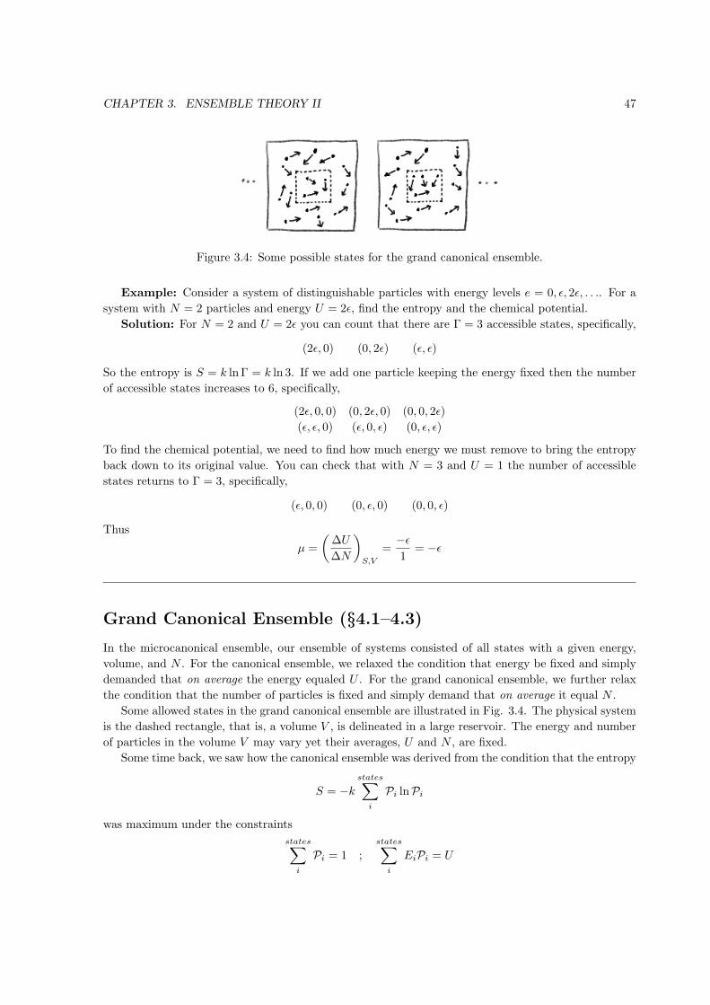
Figure 3.4: Some possible states for the grand canonical ensemble.
Example: Consider a system of distinguishable particles with energy levels e = 0, ϵ, 2ϵ, . . .. For a
system with N = 2 particles and energy U = 2ϵ, find the entropy and the chemical potential.
Solution: For N = 2 and U = 2ϵ you can count that there are Γ = 3 accessible states, specifically,
(2ϵ, 0) (0, 2ϵ) (ϵ, ϵ)
So the entropy is S = k ln Γ = k ln 3. If we add one particle keeping the energy fixed then the number
of accessible states increases to 6, specifically,
(2ϵ, 0, 0) (0, 2ϵ, 0) (0, 0, 2ϵ)
(ϵ, ϵ, 0) (ϵ, 0, ϵ) (0, ϵ, ϵ)
To find the chemical potential, we need to find how much energy we must remove to bring the entropy
back down to its original value. You can check that with N = 3 and U = 1 the number of accessible
states returns to Γ = 3, specifically,
(ϵ, 0, 0) (0, ϵ, 0) (0, 0, ϵ)
Thus
µ =
(∆U
∆N
)S,V
=−ϵ
1= −ϵ
Grand Canonical Ensemble (§4.1–4.3)In the microcanonical ensemble, our ensemble of systems consisted of all states with a given energy,
volume, and N . For the canonical ensemble, we relaxed the condition that energy be fixed and simply
demanded that on average the energy equaled U . For the grand canonical ensemble, we further relax
the condition that the number of particles is fixed and simply demand that on average it equal N .
Some allowed states in the grand canonical ensemble are illustrated in Fig. 3.4. The physical system
is the dashed rectangle, that is, a volume V , is delineated in a large reservoir. The energy and number
of particles in the volume V may vary yet their averages, U and N , are fixed.
Some time back, we saw how the canonical ensemble was derived from the condition that the entropy
S = −k
states∑i
Pi lnPi
was maximum under the constraints
states∑i
Pi = 1 ;states∑
i
EiPi = U

CHAPTER 3. ENSEMBLE THEORY II 48
where Pi is the probability of a state and Ei is the energy of a state.
For the grand canonical ensemble, states can have different numbers of particles; call Ni the number
of particles for state i. We now add an additional constraint that the average value of Ni equals N ,
that isstates∑
i
NiPi = N
Note: we use Ei for the energy of a state and U for the average energy of the system, averaged over
all states. With number of particles we use Ni and N for state and system values; hope this is not
confusing but the notation is standard and probably necessary since we are running out of letters.
Using Lagrange multipliers, as before, we obtain that S is maximum when
Pi =e−βEi+βµNi∑i
e−βEi+βµNi
Since the constraint on N is similar to the constraint on E it should not be surprising that their terms
in the above expression are similar.
The denominator in the above expression for Pi is the grand canonical partition function, Q. It is
useful to write it as
Q =
states∑i
e−βEi+βµNi
=∞∑
N=0
eβµN∑j
e−βEj (sum j is over states with Ni = N)
=
∞∑N=0
eβµNQN
where QN is the canonical partition function with N particles.
Define z = eβµ as the fugacity (sometimes called the absolute activity). Our partition function may
then be written as
Q =
∞∑N=0
zNQN
We can compute other quantities in terms of Q using the following results
U =∑i
EiPi = −(
∂
∂β
)z
lnQ
N =∑i
NiPi = z
(∂
∂z
)β
lnQ
S = −k∑i
Pi lnPi = k lnQ+ kβU − kβµN
andPV
kT= lnQ

CHAPTER 3. ENSEMBLE THEORY II 49
Example: Given the canonical partition function for a highly relativistic ideal gas of N indistin-
guishable particles to be,
QN =1
N !
[8πV (hcβ)−3
]NFind the grand canonical partition function, Q, and use it to obtain the equation of state, P (T, V,N).
Solution: Right off the bat I should mention that since we have QN we could find all the ther-
modynamic quantities directly using it; this exercise is simply to demonstrate the manipulation of
Q.
The grand canonical partition function may be written in terms of QN as,
Q =∞∑
N=0
zNQN =∞∑
N=0
1
N !
[8πV (hcβ)−3z
]NUsing
ex =∞∑
N=0
xN
N !
gives
Q = exp(8πV (hcβ)−3z)
soPV
kT= 8πV (hcβ)−3z
To replace z with N in this expression we evaluate,
N =∑i
NiPi = z
(∂
∂z
)β
= 8πV (hcβ)−3z
which yields the familiar result, P = NkT/V .
Before leaving this chapter, you might ask:
Q: For a physical system (e.g. diatomic gas, crystal, semiconductor) don’t all three ensembles (micro,
plain, and grand) give the same answer for S,U,CV , etc..?
A: Yes.
Q: Exactly the same answer?
A: Not quite, but, the differences are terms which vanish in the limit N → ∞, V → ∞, N/V fixed.
Q: So for all practical purposes, the answers are the same?
A: Yes.
Q: So why bother with three different ensembles?
A: Because depending on the problem at hand one ensemble can be much easier to work with than
another.
Q: How could the grand canonical ensemble ever be simpler since the above expression for Q involves
the canonical ensemble partition function QN?
A: You are about to see an important example. The key will be to find a trick for getting Q without
QN .
Chapter 4
Sample Exercises for First Midterm
Lecture 10The problems below are typical of midterm problems and are good exercises for review.
Problem: (a) Show that for S(T, V ),
dS =CV
TdT +
(∂P
∂T
)V
dV
(b) Show that for U(T, V ),
dU = CV dT +
[T
(∂P
∂T
)V
− P
]dV
Hint: Use part (a).
(c) Consider a van der Waals gas with molar heat capacity CV (i.e., heat capacity for one mole) and
equation of state
P =nRT
V − bn− an2
V 2
Find (∂U/∂V )T for this gas.
(d) Consider n moles of this gas undergoing free expansion from an initial state Ti, Vi to a final volume
Vf . Find the final temperature Tf .
Solution: (a) For S(T, V ),
dS =
(∂S
∂T
)V
dT +
(∂S
∂V
)T
dV
but (∂S
∂T
)V
=CV
T
(∂S
∂V
)T
=
(∂P
∂T
)V
where we used the Maxwell relation (M3).
(b) Using dU = TdS − PdV and the result from part (a) for dS gives the desired result.
(c) Comparing the mathematical expression
dU =
(∂U
∂T
)V
dT +
(∂U
∂V
)T
dV
50
CHAPTER 4. SAMPLE EXERCISES FOR FIRST MIDTERM 51
with the result from part (b) gives (∂U
∂V
)T
= T
(∂P
∂T
)V
− P
From the equation of state (∂P
∂T
)V
=nR
V − bn
so (∂U/∂V )T = an2/V 2. Notice that it is zero for an ideal gas (for which a = 0).
(d) A system does no work and exchanges no heat in a free expansion so dU = 0 and
dU =
(∂U
∂T
)V
dT +
(∂U
∂V
)T
dV = nCV dT +an2
V 2dV = 0
using the result from part (c). From this
dT = − an
CV V 2dV
so integrating both sides gives
T2 − T1 =an
CV
(1
V2− 1
V1
)Note that unlike an ideal gas, a van der Waals gas cools on expanding due to the potential energy
between the molecules. In case you’re concerned about a free expansion not being a reversible process,
remember that we’re working with exact differentials so we can always consider another path, which is
reversible, which goes from the same initial and final states and has ∆U = 0.
Problem: Consider the classical ideal gas (with N indistinguishable particles in a volume V ) in the
highly relativistic limit where the energy of a particle may be approximated as, ϵ = c(|px|+ |py|+ |pz|),where pi are the components of the momentum of the particle and c is the speed of light.
(a) Using the classical micro-canonical ensemble (fixed U , V , N), find the number of states Σ that have
energy E ≤ U . Note that the volume of a hyper-simplex in d dimensions (a pyramid whose edges are
the lines connecting the origin and the points x1 = L, x2 = L, . . ., xd = L) is Ld/d!.
(b) From the result in part (a), find U(V, T ). Note: If you could not do part (a) then take Σ = AV BUC ,
where A, B, and C are constants.
(c) From the result in part (a), find the equation of state.
(d) Find γ = CP /CV , the ratio of the heat capacities.
Solution: (a) We want to evaluate the following expression
Σ =1
N !h3N
∫dr1 . . .
∫drN
∫dp1 . . .
∫dpN
where the position integrals are constrained such that ri is within the volume V . The momentum
integrals are constrained such that
0 ≤ c(px,1 + py,1 + . . .+ pz,N ) ≤ U
CHAPTER 4. SAMPLE EXERCISES FOR FIRST MIDTERM 52
Each position integral is independent and gives a factor of V . The momentum integrals equal the
volume of a hyper-simplex with sides L = U/c and dimension d = 3N multiplied by the number of
quadrants in d dimensions, which is 2d. Thus
Σ =1
N !h3NV N 23NU3N
(3N)!c3N=
V NU3N
N !(3N)!(hc/2)3N
(b) The entropy is
S = k lnΣ = kN lnV + 3kN lnU + f(N)
where f = −k ln(N !(3N)!(hc/2)3N ). To obtain the energy in terms of temperature we may use
1
T=
(∂S
∂U
)V
=3kN
U
so U = 3kNT .
(c) The equation of state may be found using
P
T=
(∂S
∂V
)U
=kN
V
which gives ideal gas law.
(d) The heat capacity at constant volume is
CV =
(∂U
∂T
)V
= 3Nk
In general
CP = CV +TV α2
KT
where α is the coefficient of thermal expansion and KT is the isothermal compressibility. Since our
equation of state is the ideal gas law, α = 1/T and KT = 1/P , which gives CP = CV + Nk = 4Nk,
thus γ = CP /CV = 4/3. Note that for the non-relativistic ideal gas γ = 5/3.
Problem: Consider the following simple model for rubber. A chain consisting of N independent,
distinguishable links, each of length a, is attached to a weight of mass M . Each link points either
up or down; the individual links have negligible mass and kinetic energy. The energy for any given
configuration may be written as E(L) = Mg[Na−L] where the length L = a(n1 +n2 + . . .+nN ), with
ni = −1 and +1 for links pointing up and down. Find the canonical partition function, QN , and use it
to find the average length ⟨L⟩ = L(E = U) as a function of temperature. Hint: Unlike most materials,
rubber expands when cooled; you can check that your answer confirms this observation.
Solution: The partition function is
QN =
states∑e−βE =
states∑e−βMgNa exp(βMga(n1 + n2 + . . .+ nN ))
= e−βMgNa
(+1∑
n1=−1
eβMgan1
)× . . .×
(+1∑
nN=−1
eβMganN
)
= e−βMgNa
(+1∑
n=−1
eβMgan
)N
= e−βMgNa(e−βMga + eβMga
)N
CHAPTER 4. SAMPLE EXERCISES FOR FIRST MIDTERM 53
Using
U = − ∂
∂βlnQN
=∂
∂β
[βMgNa−N ln
(e−βMga + eβMga
)]= MgNa−MgNa
eβMga − e−βMga
eβMga + e−βMga
Since L(E) = Na− E/Mg,
⟨L⟩ = Na−Na+NaeβMga − e−βMga
eβMga + e−βMga
= NaeβMga − e−βMga
eβMga + e−βMga
= Na tanh(βMga) = Na tanh(Mga/kT )
Since tanh(x) increases as x increases the length increases as temperature decreases. A state of zero
entropy occurs when all the links point in the downward direction, which gives the maximum length.
Problem: Consider a classical ideal gas of N indistinguishable particles (mass m) in a rectangular
container (sides of length Lx, Ly, Lz) in a constant gravitational field with acceleration of g in the −z
direction. The container is very tall, specifically Lz ≫ LT where LT = kT/mg is the thermal height
(i.e., height at which the gravitational potential energy of a particle equals kT ).
(a) Find the classical canonical partition function, QN . You may find this integral identity helpful∫ ∞
0
e−a2x2
=
√π
2a
(b) Find the heat capacity per particle, cV = CV /N .
(c) Could the result in part (b) have been predicted from the equipartition theorem? You must justify
your answer to receive credit.
Solution: (a) The gas is ideal so the canonical partition function may be formulated as
QN =1
N !(Q1)
N
where the classical, single particle partition function is
Q1 =1
h3
∫ Lx
0
dx
∫ Ly
0
dy
∫ Lz
0
dz
∫ ∞
−∞dpx
∫ ∞
−∞dpy
∫ ∞
−∞dpz e
−βE(r,p)
where the energy is
E(r,p) =p2x2m
+p2y2m
+p2z2m
+mgz
The x and y integrals give Lx and Ly, respectively; each momentum integral is similar, for example,
1
h
∫ ∞
−∞dpxe
−p2x/(2mkT ) =
√2πmkT
h=
1
λ
CHAPTER 4. SAMPLE EXERCISES FOR FIRST MIDTERM 54
Finally, the z integral gives∫ Lz
0
dz e−βmgz =
[−1
βmge−βmgz
]Lz
0
=−1
βmg
(e−βmgLz − 1
)Since the box is tall βmgLz ≫ 1 so the exponential term is negligible and integral is approximately just
1/βmg = kT/mg = LT . Collecting these pieces gives
QN =1
N !
(LxLyLT
λ3
)N
(b) The energy of the system is
U = − ∂
∂βlnQN = −N
∂
∂βlnLT + 3N
∂
∂βlnλ = NkT +
3
2NkT =
5
2NkT
Finally, the heat capacity is
CV =
(∂U
∂T
)V
=5
2Nk
and cV = 52k.
(c) The result in part (b) could not be predicted from the equipartition theorem, as presented in
the notes and in class, because the gravitational potential energy is not quadratic in position so the
theorem does not apply. Pathria derives a more general form (eqn. (3.7.4)) for which⟨z∂E
∂z
⟩= ⟨mgz⟩ = kT
which tells us that the average potential energy for a particle is kT . Since the average kinetic energy
for a particle is 32kT we do arrive at the result obtained in part (b). Since either yes or no is a correct
answer, credit is given only when your answer is justified.
Lecture 11:
Midterm
Chapter 5
Quantum Ideal Gases
Classical LimitLecture 12
We already used the canonical ensemble to study the monatomic ideal gas using quantum mechanics
(i.e., non-interacting particles in a box). However, we had to use the approximation,
λ ≪ 3√V/N ≪ L/
3√N
Recall that
λ =h√
2πmkT
is the de Broglie wavelength of a particle at temperature T so the above inequality indicates that λ is
much smaller than the distance between particles.
This approximation puts us into the classical regime and gives us the classical result for the canonical
partition function
QN =1
N !
(V
λ3
)N
(Classical ideal gas)
The grand canonical partition function is
Q =
∞∑N=0
zNQN =
∞∑N=0
1
N !
(zV
λ3
)N
= exp
(zV
λ3
)We now return to the quantum ideal gas but without making the approximation that λ is small.
Usually when the distance between particles is comparable to their deBroglie wavelength we may no
longer neglect the interparticle forces (i.e., the gas is no longer ideal). However, there are some important
exceptions:
• Conduction electrons in a solid (λ is large because m is small).
• Photon gas (i.e., blackbody radiation).
• Liquid Helium (interatomic forces are weak).
• Ultracold systems (λ is large because T is extremely small; T ≈ 10−7).
In these cases the system of particles can be approximated as a quantum ideal gas, that is, the
interparticle forces can be neglected yet the gas cannot be treated classically.
Quantum mechanics seems to divide particles into two categories. Particles with integer spin can
have more than one particle occupying the same quantum state; these types of particles are called bosons.
55
CHAPTER 5. QUANTUM IDEAL GASES 56
Examples of such particles (and their spin) are: Alpha (0), Pion (0), Photon (1), Deuteron (1), Gluon
(1), W (1), Z0 (1). Particles with 1/2 integer spin obey an exclusion principle (Pauli exclusion). Each
quantum state can have at most one particle; these types of particles are called fermions. Examples of
such particles (and their spin) are: Electron (1/2), Muon (1/2), Proton (1/2), Neutron (1/2), Quarks
(1/2), 3He (1/2), Ω (3/2), 55Fe (3/2). Why is this the way nature works? Are there other possibilities
(i.e. anyons)? Who knows? Until other types of particles are discovered, we’ll stick with fermions and
bosons.
Fermion Grand Partition Function (§6.2)We first derive the grand partition function of fermions. Recall that this function may be written in
terms of the canonical partition function QN as
Q =∞∑
N=0
zNQN
where z = eβµ is the fugacity. While we use this definition of Q we won’t explicitly compute QN .
Start with the definition of the canonical partition function,
QN =states∑
j
e−βEj
=1∗∑
n1=0
1∗∑nz=0
. . .1∗∑
nM=0
exp (−β [n1ϵ1 + n2ϵ2 + . . .+ nM ϵM ])
where ni is the number of particles in energy state i. We have i = 1, ....,M where M is the number of
energy states (which might be infinite). The asterisks on the sums are to remind us of the constraint,
n1 + n2 + . . .+ nM = N nj = 0 or 1
that is, there are N particles distributed among the M energy states with at most one particle per
energy state.
By the way, don’t confuse system states, which are all the possible configurations of the system,
with energy states. The energy states are similar to energy levels however remember that energy states
don’t necessarily have unique energy values (i.e., ϵi = ϵj is allowed, in fact it’s common). If we picture
the classical phase space for a single particle then each energy level is a parcel in that phase space.
We can formulate our sum over system states in terms of just energy states of a single particle because
we’re still doing ideal gases where the energy of a particle only depends on its own state and not the
state of the other particles (although with quantum ideal gases, the energy states that are available to
a particle are affected by the number of particles in those energy states).
Our next step is to write QN as
QN =
(1∑
n1=0
e−βn1ϵ1
)(1∗∑
n2=0
. . .
1∗∑nM=0
exp (−β [n2ϵ2 + . . .+ nM ϵM ])
)
=(1 + e−βϵ1
)( 1∗∑n2=0
. . .
1∗∑nM=0
exp (−β [n2ϵ2 + . . .+ nM ϵM ])
)= Q
′
N +Q′
N−1e−βϵ1
CHAPTER 5. QUANTUM IDEAL GASES 57
where the prime means “remove energy state 1 from the sums.”
The grand partition function is
Q =∞∑
N=0
zNQN =
∞∑N=0
zN(Q
′
N +Q′
N−1e−βϵ1
)=
∞∑N=0
zNQ′
N + e−βϵ1z
∞∑N=1
zN−1Q′
N−1
=(1 + ze−βϵ1
) ∞∑N=0
zNQ′
N
or
Q =(1 + ze−βϵ1
)Q′
We can play the same game and pull out energy state 2 and 3 and so on. Ultimately we arrive at
Q =(1 + ze−βϵ1
) (1 + ze−βϵ2
). . .(1 + ze−βϵM
)=
M∏i=1
(1 + ze−βϵi
)which is our grand partition function for fermions.
Boson Grand Partition Function (§6.2)Our derivation here will follow the same lines as the formulation for fermions. We start with the
canonical partition function,
QN =N∗∑
n1=0
N∗∑n2=0
. . .N∗∑
nm=0
exp (−β [n1ϵ1 + . . .+ nM ϵM ])
=
(N∑
n1=0
e−βn1ϵ1
)(N∗∑
n2=0
. . .N∑
nM=0
exp (−β [n2ϵ2 + . . .+ nM ϵM ])
)Note that for bosons the sum goes from 0 to N instead of from 0 to 1. Again the ∗ means that the
sums are restricted by the condition n1 + n2 + . . .+ nM = N .
As before, we explicitly expand the n1 summation to get
QN = Q′
N + e−βϵ1Q′
N−1 + e−2βϵ1Q′
N−2 + . . .
The grand partition function is
Q =∞∑
N=0
zNQN
=∞∑
N=0
zNQ′
N + ze−βϵ1
∞∑N=1
zN−1Q′
N−1 + z2e−2βϵ1
∞∑N=2
zN−2Q′
N−2 + . . .
= (1 + ze−βϵ1 + z2e−βϵ1 + . . .)∞∑
N=0
zNQ′
N
=(1− ze−βϵ1
)−1∞∑
N=0
zNQ′
N
CHAPTER 5. QUANTUM IDEAL GASES 58
where we used the identity
1
1− a=
∞∑i=0
ai = 1 + a+ a2 + . . . |a| < 1
Next we would apply the same procedure to strip out energy state 2 then 3 and so forth. Ultimately,
we have
Q =(1− ze−βϵ1
)−1 (1− ze−βϵ2
)−1. . .(1− ze−βϵM
)−1
=M∏i=1
(1− ze−βϵi
)−1
which is our expression for the grand partition function for bosons.
General Results for Fermi and Bose Gases (§6.2–6.3)Before studying fermion and boson systems in detail, let’s obtain some general results which apply to
both types of particles.
We may write the grand partition function as
Q =
M∏i=1
(1 + σze−βϵi
)σwhere
σ =
+1, for fermions
−1, for bosons
and M is the number of energy states (which can be infinite). From this
lnQ = σM∑i=1
ln(1 + σze−βϵi
)The average number of particles in the system is
N = z
(∂
∂z
)β
lnQ = zσ
M∑i=1
σe−βϵi
1 + σze−βϵi
=
M∑i=1
(z−1eβϵi + σ
)−1 (Note: σ2 = 1
)Yet the average number of particles in an energy state, ni, is related to N as
N =M∑i=1
ni
so
ni =1
z−1eβϵi + σ
for fermions and bosons.
Some points: 1) Sometimes ni is written as ⟨ni⟩; 2) For fermions 0 ≤ ni ≤ 1 while for bosons
0 ≤ ni ≤ N ; 3) In both cases, z is fixed by the above relation for N ; 4) In the classical (high T ) limit
z ≪ 1 so ni ≈ exp(−βϵi), which gives the Maxwell-Boltzmann distribution.

CHAPTER 5. QUANTUM IDEAL GASES 59
The energy is
U = −(
∂
∂β
)z
lnQ =M∑i=1
ϵiz−1eβϵi + σ
=M∑i=1
niϵi
Many of our calculations for Fermi and Bose ideal gases will involve either the above expression for N
or the expression for U .
Fermi and Bose Integrals (§7.1, 8.1, Appendices D,E)Lecture 13
We now have the grand partition function for quantum ideal gases,
Q =M∏i=1
(1 + σze−βϵi
)σwhere
σ =
+1, for fermions
−1, for bosons
We also have
PV
kT= lnQ = σ
M∑i=1
ln(1 + σze−βϵi
)and
N = z
(∂
∂z
)β
lnQ =
M∑i=1
ze−βϵi/(1 + σze−βϵi
)and
U = −(
∂
∂β
)z
lnQ = −(
∂
∂β
)z
PV
kT
We could write other thermodynamic variables in terms of lnQ but the above are the most useful.
While the above is complete, the sums are clumsy to work with. For this reason we will convert
from sums over energy states (taking M → ∞) to integrals over phase space,
M∑i=1
→ gdh3
∫r
∫dp
=gdh3
(V )
2π∫0
dϕ
π∫0
dθ sin θ
∞∫0
dp p2
=
4πgdh3
V
∞∫0
dp p2
where gd is the degeneracy factor (number of states that have the same energy). Since our only
integration is over momentum, we rewrite the energy of a state using ϵ = p2/2m (which is legit as long
as our particles do not move at relativistic speeds).
We are not reverting back to classical mechanics even though the notation is similar. Physical
systems have many particles so there are a large number of states; the only approximation that we are
making here to assume that systems have so many states that we can replace the sums with integrals.
Our previous classical limit was a high temperature approximation.
CHAPTER 5. QUANTUM IDEAL GASES 60
Our expressions are now
P
kT= gd
4π
h3σ
∫ ∞
0
dp p2 ln(1 + σze−βp2/2m
)and
N
V= gd
4π
h3
∫ ∞
0
dp p2ze
−βp2/2m
1 + σze−βp2/2m
Our previous classical approximation, taking z ≪ 1 and using ln(1 + x) ≈ x, we would write these
expressions as
P
kT≈ gd
4π
h3σ
∫ ∞
0
dp p2σze−βp2/2m
=gdz
λ3(Classical approximation)
which agrees with our earlier result, lnQ = PV/kT = zV/λ3, for nondegenerate (gd = 1) energy states.
Similarly, the classical approximation gives
N
V≈ gd
4π
h3σ
∫ ∞
0
dp p2σze−βp2/2m
=gdz
λ3(Classical approximation)
which using the previous equation gives PV = NkT .
We introduce the Fermi integrals
f5/2 (z) =4√π
∫ ∞
dxx2 ln
(1 + ze−x2
)=
∞∑ℓ=1
(−1)ℓ+1zℓ
ℓ5/2
f3/2 (z) = z∂
∂zf5/2(z)
=∞∑ℓ=1
(−1)ℓ+1zℓ
ℓ3/2
For fermions, we thus have
P
kT=
gdλ3
f5/2 (z)
N
V=
gdλ3
f3/2 (z)
which are equations (8.1.3) and (8.1.4) in Pathria (see pg. 231).
Similarly, we introduce the Bose integrals,
g5/2 (z) = − 4√π
∫ ∞
0
dxx2 ln(1− ze−x2
)=
∞∑ℓ=1
zℓ
ℓ5/2
g3/2 (z) = z∂
∂zg5/2 (z)
=∞∑ℓ=1
zℓ
ℓ3/2

CHAPTER 5. QUANTUM IDEAL GASES 61
so for bosons,
P
kT=
gdλ3
g5/2 (z)
N
V=
gdλ3
g3/2 (z)
Careful: don’t confuse gd with the Bose integrals; sorry but this is the standard notation.
If you compare the above with equations (7.1.5) and (7.1.6) in Pathria (pg. 180) you will find a
discrepancy. We should actually write
P
kT=
1
λ3g5/2 (z)−
1
Vlog (1− z)
N
V=
1
λ3g3/2 (z) +
1
V
z
1− z
The last term in each expression is a correction required for very low temperature problems. Since the
origin of these corrections is intellectually interesting we return to this question later and consider it in
some depth.
We may also write the internal energy in terms of the above integrals. Using
U = −(
∂
∂β
)z
lnQ = −(
∂
∂β
)z
PV
kT
Since dλ/dβ = λ/2β, from our previous results,
U =3
2gdV
kT
λ3×f5/2(z), (Fermi)
g5/2(z), (Bose)
We also find
U =3
2PV (both Bose and Fermi)
a result which is also true for the classical monatomic ideal gas.
Fermi Energy
We now consider a Fermi gas in some detail. Using the grand canonical ensemble, we already determined
thatN
V=
gdλ3
f3/2 (z)
where λ = h/√2πmkT is the thermal wavelength and z = eβµ is the fugacity. You should view this
expression as an equation to obtain z, or equivalently, to give the chemical potential µ, given T , V , and
N .
The Fermi function f3/2 (z) may be written as
f3/2 (z) =4√π
∫ ∞
0
dxx2
z−1ex2 + 1=
∞∑ℓ=1
(−1)ℓ+1
zℓ
ℓ3/2
Figure 5.1 shows a sketch of this function. We will be interested in the approximations
f3/2 (z) ≈z, z ≪ 14
3√π(log z)
3/2, z ≫ 1
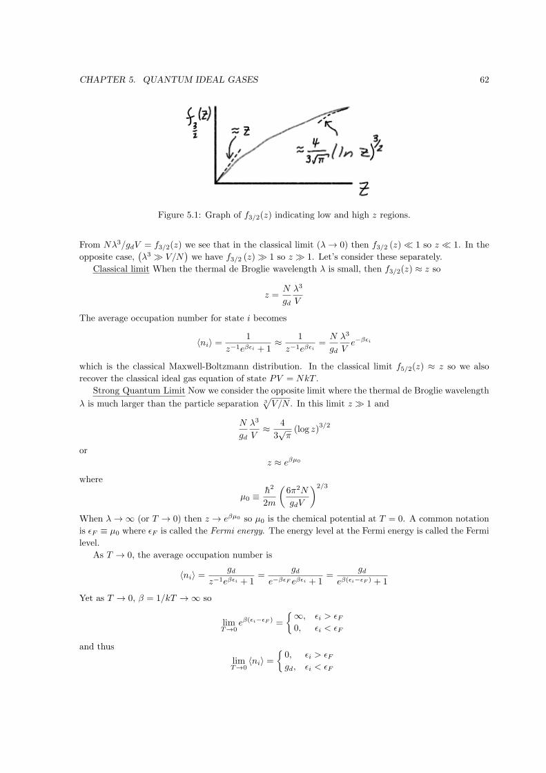
CHAPTER 5. QUANTUM IDEAL GASES 62
Figure 5.1: Graph of f3/2(z) indicating low and high z regions.
From Nλ3/gdV = f3/2(z) we see that in the classical limit (λ → 0) then f3/2 (z) ≪ 1 so z ≪ 1. In the
opposite case,(λ3 ≫ V/N
)we have f3/2 (z) ≫ 1 so z ≫ 1. Let’s consider these separately.
Classical limit When the thermal de Broglie wavelength λ is small, then f3/2(z) ≈ z so
z =N
gd
λ3
V
The average occupation number for state i becomes
⟨ni⟩ =1
z−1eβϵi + 1≈ 1
z−1eβϵi=
N
gd
λ3
Ve−βϵi
which is the classical Maxwell-Boltzmann distribution. In the classical limit f5/2(z) ≈ z so we also
recover the classical ideal gas equation of state PV = NkT .
Strong Quantum Limit Now we consider the opposite limit where the thermal de Broglie wavelength
λ is much larger than the particle separation 3√V/N . In this limit z ≫ 1 and
N
gd
λ3
V≈ 4
3√π(log z)
3/2
or
z ≈ eβµ0
where
µ0 ≡ h2
2m
(6π2N
gdV
)2/3
When λ → ∞ (or T → 0) then z → eβµ0 so µ0 is the chemical potential at T = 0. A common notation
is ϵF ≡ µ0 where ϵF is called the Fermi energy. The energy level at the Fermi energy is called the Fermi
level.
As T → 0, the average occupation number is
⟨ni⟩ =gd
z−1eβϵi + 1=
gde−βϵF eβϵi + 1
=gd
eβ(ϵi−ϵF ) + 1
Yet as T → 0, β = 1/kT → ∞ so
limT→0
eβ(ϵi−ϵF ) =
∞, ϵi > ϵF0, ϵi < ϵF
and thus
limT→0
⟨ni⟩ =0, ϵi > ϵFgd, ϵi < ϵF

CHAPTER 5. QUANTUM IDEAL GASES 63
In other words, as T → 0, all states below the Fermi level are filled and all states above the Fermi level
are empty. The particles filling the energy levels below ϵF are called the “Fermi sea” (a better term
would be the “Fermi Seventh Street Garage During the First Week of Classes”).
From the Fermi energy we can define a Fermi temperature as ϵF = kTF or TF = ϵF /k. If T ≫ TF ,
then the system is in the classical regime. However, for most fermi gases of interest, T ≪ TF so they
are in the strong quantum limit.
It is easy to understand why the chemical potential at T = 0 equals the Fermi energy. At T = 0,
every fermion is in its lowest possible energy level and stacked, due to Fermi exclusion, up to the Fermi
level. The entropy is zero at T = 0; there is only one possible state for the system. Now add a single
particle; this particle has to be place on the stack at the next available energy level. This means that
the particle will have infinitesimally more energy than the Fermi energy. But the entropy remains zero
so the energy of the system increases by ϵF thus the chemical potential
µ =
(∂U
∂N
)S,V
= ϵF (T = 0)
It turns out that µ ≈ 0 for T ≈ TF and the chemical potential is negative when T ≫ TF , which was
already pointed out for the classical ideal gas.
The chemical potential at T = 0 is µ0 = ϵF ; to obtain µ for T > 0, we need to keep the next order
in the expansion for f3/2 (z). Specifically,
f3/2(z) =4
3√π(log z)
3/2
[1 +
π2
8(log z)
−2+ . . .
]≈ 4
3√π(βµ)
3/2
[1 +
π2
8(βµ)
−2
](z ≫ 1)
Using this new approximation we get,
Nλ3
gdV=
4
3√π(βµ)
3/2
[1 +
π2
8(βµ)
−2
]or
(βµ)3/2
=3√π
4
Nλ3
gdV
[1 +
π2
8(βµ)
−2
]−1
or
µ =1
β
(3√π
4
Nλ3
gdV
)2/3 [1 +
π2
8(βµ)
−2
]−2/3
= ϵF
[1 +
π2
8(βµ)
−2
]−2/3
Only one hitch, we have µ in the correction term on the r.h.s.. However, since that term is the first
order correction, we set µ = µ0 = ϵF on the r.h.s. and get
µ ≈ ϵF
[1 +
π2
8(βϵF )
−2
]−2/3
≈ ϵF
[1− π2
12(βϵF )
−2
]= ϵF
[1− π2
12
(kT
ϵF
)2]
= ϵF
[1− π2
12
(T
TF
)2]
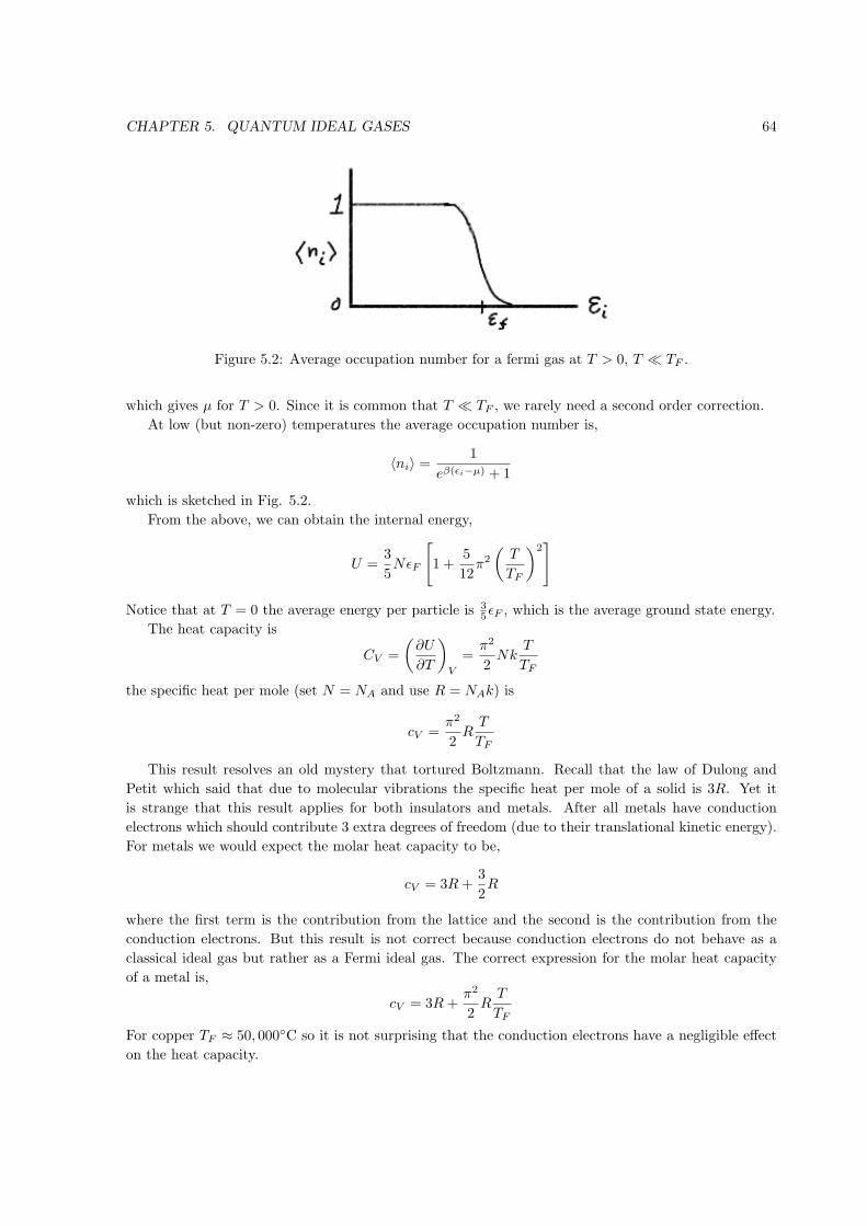
CHAPTER 5. QUANTUM IDEAL GASES 64
Figure 5.2: Average occupation number for a fermi gas at T > 0, T ≪ TF .
which gives µ for T > 0. Since it is common that T ≪ TF , we rarely need a second order correction.
At low (but non-zero) temperatures the average occupation number is,
⟨ni⟩ =1
eβ(ϵi−µ) + 1
which is sketched in Fig. 5.2.
From the above, we can obtain the internal energy,
U =3
5NϵF
[1 +
5
12π2
(T
TF
)2]
Notice that at T = 0 the average energy per particle is 35ϵF , which is the average ground state energy.
The heat capacity is
CV =
(∂U
∂T
)V
=π2
2Nk
T
TF
the specific heat per mole (set N = NA and use R = NAk) is
cV =π2
2R
T
TF
This result resolves an old mystery that tortured Boltzmann. Recall that the law of Dulong and
Petit which said that due to molecular vibrations the specific heat per mole of a solid is 3R. Yet it
is strange that this result applies for both insulators and metals. After all metals have conduction
electrons which should contribute 3 extra degrees of freedom (due to their translational kinetic energy).
For metals we would expect the molar heat capacity to be,
cV = 3R+3
2R
where the first term is the contribution from the lattice and the second is the contribution from the
conduction electrons. But this result is not correct because conduction electrons do not behave as a
classical ideal gas but rather as a Fermi ideal gas. The correct expression for the molar heat capacity
of a metal is,
cV = 3R+π2
2R
T
TF
For copper TF ≈ 50, 000C so it is not surprising that the conduction electrons have a negligible effect
on the heat capacity.
CHAPTER 5. QUANTUM IDEAL GASES 65
An alternative way to view this phenomenon is to consider the other definition of heat capacity
CV = T
(∂S
∂T
)V
As temperature increases, only a few particles rise above their ground states. Most particles remain in
the ground state so long as T ≪ TF . For this reason, the number of accessible states Γ (and consequently
the entropy S) increases very slowly. Since(∂S∂T
)V
is small, so is CV .
Finally, the pressure in a Fermi gas is
P =2
3
U
V=
2
5
NϵFV
[1 +
5π2
12
(T
TF
)2]
Notice that even when T = 0, the pressure is nonzero. Again this is due to the ground state energy of
the particles. In the next section we consider an example in which this pressure supports a star and
prevents its gravitational collapse.
White Dwarf Stars (§8.5)Lecture 14
We now consider an interesting example of a Fermi gas. White dwarf stars have long been recognized
as unusual in that they are exceptionally faint given their color. It is well established that this is due to
their old age; in a white dwarf most of the hydrogen has been fused into heavier elements (outer shell
is helium while the core is mostly carbon, oxygen and nughat).
From various types of measurements, we know that a typical white dwarf has a density of ρ ≈107g/cm
3(10 million times the density of water) and temperature T ≈ 107K (about the temperature of
the sun). Interestingly, because the density is high, the Fermi temperature of the electrons is TF ≈ 1011
K. Since T ≪ TF almost all the electrons are in their ground state. The star’s temperature is relatively
“cold” and we can treat the electrons as a Fermi gas in its ground state.
A star is an interesting container of gas. It has no outer wall but rather it relies on gravitational
attraction to contain its gas. We may view the gravitational force as exerting a pressure, just as the
walls of an ordinary container.
The question we now want to answer is: knowing the theory for a Fermi gas, what is the radius of
a white dwarf given its mass? That is, at what radius does the pressure of the Fermi gas balance the
gravitational force?
First, let’s derive the results we need for a Fermi gas of electrons, (Note: we could work out
the pressure contribution for the helium nuclei but would find it to be negligible compared with the
electrons).
Unfortunately, our derivation for a Fermi gas assumed nonrelativistic dynamics (i.e., we used ϵ =12mv2 = p2/2m). However, we must now use the relativistic expression
ϵ =
√(pc)2 + (mc2)
2
Fortunately, we can assume that all the electrons are in their ground state (since T ≪ TF ).
The total internal energy is then
U = gd
states∑i
ϵini
CHAPTER 5. QUANTUM IDEAL GASES 66
with the number of electrons in state i being
ni =
1, if ϵi < ϵF0, if ϵi > ϵF
Electrons are spin 12 so each energy state (level) can contain two electrons, a spin up and a spin down,
so gd = 2.
We define a Fermi momentum pF as the momentum of a particle with Fermi energy. Since every
state up to the Fermi level is filled,
N = 2∑r
∑p≤pF
1
= 2
(1
h3
∫dr
∫dp
)=
2V
h3(4π)
∫ pF
0
dp p2 =8πV
h3
p3F3
so
pF = h
(3π2N
V
)1/3
The total energy in the gas is found by summing up the energy of all the particles,
U = 2∑r
∑p<pF
ϵ (r, p)
As usual, we replace the sum over states with an integral over states by integrating over position and
momentum,
U = 21
h3
∫V
dr
∫p<pF
dp
√(pc)
2+ (mc2)
2
= 21
h3(V ) (4π)
pF∫0
dp p2√(pc)
2+ (mc2)
2
or
U =m4c5
π2h3 V f (xF )
where xF ≡ pF /mc and
f(x) ≡∫ x
0
dy y2√1 + y2 =
1
8
√x2 + 1(2x3 + x)− 1
8sinh−1(x)
Note that f(x) is no a particularly interesting looking function; it basically looks like xa where a is a
small integer (around 2 to 5 depending on whether x → 0 or x → ∞).
The reason we wanted to get U is that we can get the pressure using
P = −(∂U
∂V
)S
Note: Entropy is fixed because all electrons are in the ground state. Putting in our expression for U ,
P = −(m4c5
π2h3
)[f (xF ) +
∂f
∂xF
(∂xF
∂V
)S
]=
(m4c5
π2h3
)[1
3x3F
√1 + x2
F − f (xF )
]
CHAPTER 5. QUANTUM IDEAL GASES 67
This gives us pressure in terms of xF but we would prefer to know in terms of M , the star’s mass
and R, the star’s radius. Yet it is simple to write xF in terms of M and R since
xF =pFmc
=h
mc
(3π2N
V
)1/3
=M
1/3
R
where
R =R
h/mc
is a dimensionless radius and
M =9π
8
M
mp
is a dimensionless mass. We’ve used the fact that the star’s mass, M , is related to the number of
electrons, N , as
M ≈ 2mpN
where mp is the mass of a proton. That is for each electron there is approximately one proton and one
neutron (which have about the same mass). All miscellaneous constants are stuffed into M and R to
keep things tidy.
Our expression for the pressure remains complicated. However, in the two approximations
P ≈ 4
5Kx5
F (xF ≪ 1)
and
P ≈ K(x4F − x2
F
)(xF ≫ 1)
where
K =mc2
12π
(mc
h
)3we use these expressions in a moment.
The gravitational force of the star must balance the pressure of the Fermi gas in order to contain
the gas. To do this right, the calculation requires solving some partial differential equations. Yet we
can use a simple approximation for the pressure exerted by gravity.
(Force) = − ∂
∂R(gravitational potential energy)
P × (surface area) = − ∂
∂R
(−GM2
R
)P(4πR2
)=
GM2
R2
so
P =1
4π
GM2
R4
Comparing this with our previous expression for pressure allows us to solve for radius in terms of
mass. We find,
1) In the low density limit (xF ≪ 1),
R ∝ M−1/3
Notice that as mass increases, radius decreases.
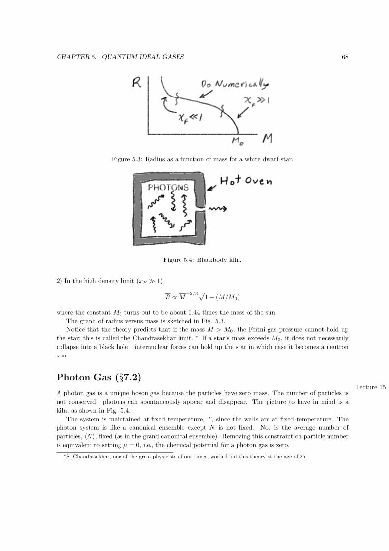
CHAPTER 5. QUANTUM IDEAL GASES 68
Figure 5.3: Radius as a function of mass for a white dwarf star.
Figure 5.4: Blackbody kiln.
2) In the high density limit (xF ≫ 1)
R ∝ M−2/3√
1− (M/M0)
where the constant M0 turns out to be about 1.44 times the mass of the sun.
The graph of radius versus mass is sketched in Fig. 5.3.
Notice that the theory predicts that if the mass M > M0, the Fermi gas pressure cannot hold up
the star; this is called the Chandrasekhar limit. ∗ If a star’s mass exceeds M0, it does not necessarily
collapse into a black hole—internuclear forces can hold up the star in which case it becomes a neutron
star.
Photon Gas (§7.2)Lecture 15
A photon gas is a unique boson gas because the particles have zero mass. The number of particles is
not conserved—photons can spontaneously appear and disappear. The picture to have in mind is a
kiln, as shown in Fig. 5.4.
The system is maintained at fixed temperature, T , since the walls are at fixed temperature. The
photon system is like a canonical ensemble except N is not fixed. Nor is the average number of
particles, ⟨N⟩, fixed (as in the grand canonical ensemble). Removing this constraint on particle number
is equivalent to setting µ = 0, i.e., the chemical potential for a photon gas is zero.
∗S. Chandrasekhar, one of the great physicists of our times, worked out this theory at the age of 25.
CHAPTER 5. QUANTUM IDEAL GASES 69
The canonical partition function is
Q =
∞∑n1=0
∞∑ni=0
. . .
∞∑nM=0
exp (−βE (n1, n2, . . . , nM ))
where ni is the number of photons in energy level i and E is the energy for the state (n1, . . . , nM ).
Notice that the sums are unrestricted since particle number is unconstrained.
Call ϵi the energy of a photon in state i and we may write
Q =∞∑
n1=0
. . .∞∑
nM=0
e−β[n1ϵ1+n2ϵ2+...+nM ϵM ]
=
( ∞∑n1=0
e−βn1ϵ1
)( ∞∑n2=0
e−βn2ϵ2
). . .
( ∞∑nM=0
e−βnM ϵM
)
=
(1
1− e−βϵ1
)(1
1− e−βϵ2
). . .
(1
1− e−βϵM
)=
M∏i=1
1
1− e−βϵi
so
lnQ = −M∑i=1
ln(1− e−βϵi
)Notice how easy those unrestricted sums were. For photons there is no physical upper bound on the
number of states so we may take M = ∞.
As usual, to get much farther we need to replace the sum over states into integrals over phase space,
states∑→
spins∑ 1
h3
∫V
dr
∫dp
= (2)1
h3(V )
∫dp
=8πV
h3
∫ ∞
0
dp p2
since there are two spin states (corresponding to left and right polarized).
One usually prefers characterizing the state of a photon by its frequency rather than its momentum
so using p = ϵ/c = hω/c,8πV
h3
∫ ∞
0
dp p2 → V
π2c3
∫ ∞
0
dω ω2
and
lnQ = − V
π2c3
∫ ∞
0
dω ω2 ln(1− e−βhω
)=
π2V
45c3
(kT
h
)3
The pressure may be found using PV = kT lnQ, and
P =π2
45c3h3 (kT )4=
4
3σT 4
CHAPTER 5. QUANTUM IDEAL GASES 70
where σ is Stefan’s constant.
The energy is
U = −(
∂
∂βlnQ
)V
= 4σV T 4
so PV = 13U .
For our final result, go back a moment to our integral expression for lnQ,
lnQ = − V
π2c3
∫ ∞
0
dω ω2 ln(1− e−βhω
)Using U = −
(∂∂β
)VlnQ
U =V
π2c3
∫ ∞
0
dω ω2 hωe−βhω
1− e−βhω
orU
V=
∫ ∞
0
dω u(ω, T )
where
u(ω, T ) =h
π2c3ω3
eβhω − 1
is the energy per unit volume per unit frequency, i.e., the Planck radiation law (see Fig. 7.7 in Pathria).
By the correspondence principle, in the limit, h → 0, eβhω ≃ 1 + βhω, we recover the classical
Rayleigh-Jeans law
u (ω, T ) =kT
π2c3ω2
The ultraviolet catastrophe (u → ∞ as ω → ∞) in the classical result led to the birth of quantum
mechanics.
Phonons in Solids (§7.3)The sound modes in a solid can be analyzed in a fashion very similar to blackbody radiation. This
similarity is suggested by the name “phonon” which is a quantized vibrational excitation.
Just as with photons, our partition function is
lnQ = −M∑i=1
ln(1− e−βϵi
)= −
M∑i=1
ln(1− e−βhωi
)Yet there are some differences. First, the number of states (i.e., modes), M , is not infinite but rather
is limited to 3N , where N is the number of atoms in the solid. This limitation may be understood by
the fact that the smallest wavelength of the sound modes is bounded by the finite separation between
atoms.
As before, we want to replace the sum over states with an integral and this is as with photons,
M∑i=1
→ 3
2
V
π2c3
∫ ωmax
0
dω ω2
with the following differences:

CHAPTER 5. QUANTUM IDEAL GASES 71
(1) The polarization vector for phonons has 3 directions (2 traverse + 1 longitudinal) instead of 2
(just transverse) as with photons. This produces the factor 3/2.
(2) The speed c is the sound speed instead of the speed of light
(3) The finite number of modes introduces a maximum frequency ωmax. This ωmax is found using
the condition,3
2
V
π2c3
∫ ωmax
0
dω ω2 = 3N
or
ωmax = c
(6π2N
V
)1/3
for the maximum frequency.
I should mention that we have made an approximation (first introduced by Debye) that the distri-
bution of modes is the same as for photons. In reality, we should write
M∑i=1
→∫ ωmax
0
f (ω) dω
where f (ω) is the density of states.
The partition function, using the Debye approximation, is
lnQ = − 3V
2π2c3
∫ ωmax
0
ln(1− e−βhω
)ω2 dω
The internal energy is
U = −(
∂
∂βlnQ
)V
=3V
2π2c3
∫ ωmax
0
dω ω2 hω
eβhω − 1
= 9N(kT )
4
(hωmax)3
∫ βhωmax
0
t3
et − 1dt
This last integral is tabulated (see Debye function). If we define a Debye temperature T0 = hωm/k
then we have the approximations,
U = 3NkT ×
1− 38T0
T + . . . , T ≫ T0
π2
5
(TT0
)3+ . . . , T ≪ T0
Typically, T0 ≈ 200K so at room temperature U ≈ 3NkT and CV =(∂U∂T
)V≈ 3Nk = 3Rn, where n is
the number of moles. This last expression is the familiar law of Dulong and Petit. For low temperatures,
U ∝ T 4 so CV ∝ T 3, as seen experimentally.
Bose-Einstein Condensation (§7.1-2)Lecture 16
We already worked out the grand partition function for bosons,
Q =states∏
i
(1− ze−βϵi
)−1
CHAPTER 5. QUANTUM IDEAL GASES 72
where ϵi is the energy of state i. We also have
PV
kT= lnQ = −
states∑i
ln(1− ze−βϵi
)
N = z∂
∂zlnQ =
states∑i
ze−βϵi
1− ze−βϵi
Normally, we replace the sums over states with integrals over phase space
states∑i
→ 4π
h3V
∫ ∞
0
dp p2
so, for example
N =4π
h3V
∫ ∞
0
dp p2ze−βp2/2m
1− ze−βp2/2m
=V
λ3g3/2 (z)
where the function g3/2 (z) is the Bose integral we met before.
I already mentioned that, in some cases, this replacement of the sum over states was not a good
approximation and had to be modified. Let’s consider why.
An aside: For bosons, 0 ≤ z < 1. You can prove this by considering the average occupation number
ni =1
z−1eβϵi − 1=
z
eβϵi − z
For the ground state, i = 1, ϵ1 = 0, we have
n1 =z
1− z
Since 0 ≤ n1 < ∞, the fugacity must be between 0 and 1. (Note: for fermions 0 ≤ z < ∞.)
Consider the bose integral g3/2 (z) in its summation form,
g3/2 (z) =
∞∑l=1
zl
l3/2
It is easy to show that
maxg3/2 (z)
= g3/2 (1) = ζ (3/2) ≃ 2.612
See Fig. 12.3 in Huang for a graph of g3/2 (z).
Now for the paradox. Since the thermal wavelength is
λ =h√
2πmkT
then λ → ∞ as T → 0. Yet if
N =V
λ3g3/2 (z)
then N → 0 as T → 0, that is, the number of particles in the system goes to zero as the temperature
goes to zero. Weird. As one author (Robertson) puts it
CHAPTER 5. QUANTUM IDEAL GASES 73
“. . . not even the magic of quantum mechanics can make particles disappear with cooling
or reappear when warmed.”
The key to resolving this paradox is to realize that at low temperatures, a significant fraction of the
particles will occupy the ground state. We explicitly separate the first term from the sum over states,
and replace the remaining sum with an integral, as before,
N =
∞∑i=1
1
z−1eβϵi − 1
=1
z−1 − 1+
∞∑i=2
1
z−1eβϵi − 1
=z
1− z+
V
λ3g3/2 (z)
= Ngr (z) +Nex (z)
where Ngr, Nex are the number of particles in the ground state and non-ground states respectively. As
we saw, the Nex → 0 as T → 0 yet the first term, Ngr = z/ (1− z) can be arbitrarily large as z → 1.
As we saw, the maximum value for g3/2 (z) is ζ (3/2) (≃ 2.612) so the maximum number of particles
outside the ground state is
max Nex (z) =V
λ3ζ (3/2) = Nex (z = 1)
Recall that λ ∝ T−3/2; we define a critical temperature, Tc, by the condition,
Nex (1) = N
orV
λ(Tc)3ζ (3/2) = N
In other words, we ask: at what minimum temperature could we still fit all the particles into non-ground
states? Solving the above for this temperature
kTc =
(h2
2πm
)(N
V ζ (3/2)
)2/3
By the way, the value of kTc is approximately the same as the Fermi energy so quantum effects appear
in the same energy range for fermions and bosons.
The graph of Ngr and Nex is shown in Fig. 5.5. Specifically, the functions are
Ngr =
N(1− (T/Tc)
3/2), T < Tc
0, T > Tc
Notice that below T = Tc, particles start collecting in the ground state; this phenomenon is called
Bose-Einstein condensation.
To obtain the other thermodynamic properties, we use the standard expressions but treat the ranges
T < Tc and T > Tc separately:
• For T < Tc: The value of z in this case is very close to 1. For example, if the ground state contains a
mere 106 particles then from
Ngr =z
1− z

CHAPTER 5. QUANTUM IDEAL GASES 74
Figure 5.5: The number of particles in the ground state and in excited states as a function of tempera-
ture.
we have that z ≈ 0.999999. Thus for T < Tc, we may set z = 1 everywhere except the above expression
for Ngr.
• For T > Tc: We can take Ngr = 0, Nex = N so
N =V
λ3g3/2 (z)
We must solve this expression to find z; probably need to do this numerically.
Some of the other thermodynamic results we obtain from the partition function include
U =
32kT
Vλ3 g5/2 (z) , (T > Tc)
32kT
Vλ3 g5/2 (1) , (T < Tc)
(see Fig. 7.10b in Pathria and Beale) and
CV =
15R4
g5/2(z)
g3/2(z)− 9R
4
g3/2(z)
g1/2(z)(T > Tc)
15R4
g5/2(1)
g3/2(1)
(TTc
)3/2(T < Tc)
Graphing the specific heat, we get a curve with a noticeable cusp; see Fig. 5.6 or Pathria and Beale’s
Fig. 7.11. Quantum effects in a Fermi gas of electrons are significant, even at room temperature, because
the mass of an electron is small, giving it a large deBroglie wavelength. We don’t have a similar situation
for bosons. For a He4 atom (spin 0), the critical temperature at which Bose-Einstein condensation would
occur is Tc = 2.18K. Experimentally, at T = 3.14K, He4 does have a phase transition into a superfluid
phase. The specific heat near the transition is reminiscent of the ideal Bose gas result. Unfortunately,
a liquid is not well approximated as an ideal gas; the interaction between atoms is not negligible. Thus
our B-E condensation is only a first step toward understanding superfluid helium.
Bose-Einstein condensation is observed in the laboratory † and significant experimental work has
been done in the field of quantum ideal gases in the past decade. Finally, white dwarfs are filled with
helium nuclei and are so dense that the critical temperature is quite high(Tc ≈ 2.5× 10⁶K
). Maybe we
have B-E condensation in their cores? There is a white dwarf nearby (8 light years away, near Sirius),
we should go check this out.
†M.H. Anderson, J.R. Ensher, M.R. Matthews, C.E. Wieman, and E.A. Cornell, Science 269 198 (1995).

CHAPTER 5. QUANTUM IDEAL GASES 75
Figure 5.6: Heat capacity of an ideal boson gas as a function of temperature; notice cusp at T = Tc.
Chapter 6
Non-ideal Systems – Ising Model
Ideal vs. Non-ideal Systems §12.3Lecture 17
Statistical mechanics has given us a general recipe for obtaining thermodynamic properties given the
microscopic dynamics of a system. For example, using the canonical ensemble, one computes the
partition function
QN =states∑
i
e−βEi
and obtain all thermodynamics from this.
Thus far we have concentrated on ideal systems, that is, systems where the energy of each state was
a sum over the energy of each particle
Ei = ϵ1(j′) + ϵ2(j
′′) + . . .+ ϵN (j′ · · ·′)
and the energy of each particle is independent of the state of the other particles. For distinguishable
particles, the partition function simplifies
QN =
states∑j
e−βϵ1(j)
︸ ︷︷ ︸
Particle 1
× . . .×
states∑j
e−βϵN (j)
︸ ︷︷ ︸
Particle N
= (Q1)N
where Q1 is the partition function for a single particle. Sometimes counting states is a little more
difficult (e.g., Fermi and Bose ideal gases) but still doable within one lecture.
In this chapter we consider the much more difficult problem of non-ideal systems for which the
energy does not decompose as a simple sum of single particle energies because of interactions between
the particles.
To give you a picture to have in mind, consider the following two examples:
Classical Non-ideal Gas In this system the energy of a single particle has both a kinetic and potential
energy contribution,
ϵi =1
2mp2i +
N∑k =i
U(|qi − qk|)
76

CHAPTER 6. NON-IDEAL SYSTEMS – ISING MODEL 77
where U is the potential energy due to the force between a pair of particles, which is here taken to only
be a function of their relative separation. The total energy for a given state is
E(q1, . . . , qN , p1, . . . , pN ) =N∑i=1
ei(q1, . . . , qN , pi)
This system is not an ideal gas, that is,
E(q1, . . . , qN , p1, . . . , pN ) =N∑i=1
ei(qi, pi)
because the potential energy for particle j is a function of the positions of all the other particles.
Quantum Ising Spin System Consider a lattice of particles with spin 12 for which the state of particle
i is si = +1 (“up”) or −1 (“down”).∗ Two typical configurations could be pictured as
+ + − +
− + − −+ + − +
+ − + −
+ + − +
+ + + +
+ − + +
+ + + +
In the left configuration the spins appear randomly oriented while on the right they are aligned to
mostly point up. The state of the system is given by the set of quantum numbers (s1, . . . , sN ).
The spins interact in this system and we write the total energy for a given state as
E(s1, . . . , sN ) =1
2
N∑i=1
N∑j=1
Uij(si, sj) +N∑i=1
UHi (si)
where Uij is the potential energy due to the interaction between spins i and j; UHi is the potential
energy of spin i in the presence of an external magnetic field H.
The Ising model simplifies this system even further to write the energy as
E(s1, . . . , sN ) = −1
2
N∑i=1
γ∑j∈Ni
ϵsisj −N∑i=1
Hsi
where the sum “j ∈ Ni” is restricted to the spins that are “neighbors” of spin i; each spin has γ
neighbors.† The interaction energy is ϵ so if ϵ > 0 then the lower energy state is when spins are aligned
(si and sj both +1 or both −1). The potential energy due to the external field is also lower when H
and si have the same sign (i.e., when the spin points in the same direction as the field).
The Ising model is a simplified representation of a ferromagnet. You can check that the energy
cannot be written as the sum of independent terms, that is,
E(s1, . . . , sN ) =N∑i=1
e(si)
because of the nonlinear interaction between the spins. The Ising model is non-ideal system due to the
coupling of a spin and its neighbors. Despite its simplicity it is a very rich theoretical model since it is
one of the simplest non-ideal systems with a direct relation to a physical material.
∗NOTATION: Pathria uses σi instead of si†NOTATION: Pathria uses J instead of ϵ and µB instead of H

CHAPTER 6. NON-IDEAL SYSTEMS – ISING MODEL 78
Approaches for Non-ideal Systems
Now that we’ve seen the general form and two examples of non-ideal systems, let’s consider some ways
of tackling these problems.
Brute Force Approach One way to proceed would be to numerically evaluate the partition function
QN using its definition as a sum over states. This turns out to be impractical; let’s see why.
Consider the Ising model for a small three-dimensional system with 10×10×10 lattice sites (N = 1000
spins). The partition function is
QN =states∑
i
e−βEi
=+1∑
s1=−1
+1∑s2=−1
. . .+1∑
sN=−1
exp(−βE(s1, s2, . . . , sN ))
Each sum has only two terms but there are 1000 sums so the total number of terms to evaluate is
21000 ≈ 10300.
Modern supercomputers can evaluate about 1015 operations per second (1 Petaflop). Even if each
term required only one operation, this small system would require 10285 s ≈ 10275 years to evaluate QN
for a single value of β!
Phenomenological Approach This approach can be generously termed “intelligent guessing” or cyn-
ically termed “fudging to fit the answer.” The paradigm for this approach is the formulation of the van
der Waals model for dense gases and liquids. Starting from the ideal gas, van der Waals proposed two
corrections to account for the short-ranged repulsion force and the long-ranged attraction force. For
many phenomena (e.g., behaviour near the gas-liquid critical point) the model is in good agreement
with experimental data, indicating that it contains some elements of truth.
The phenomenological approach produces thermodynamic models that are only partially derived
from statistical mechanics. This is less satisfying to the pure theorist but the models can be very handy
for general applications. And sometimes the model can be derived from fundamental principles, as with
the Kac-Uhlenbeck-Hemmer analysis of the van der Waals model, thought this usually takes decades
(90 years for the van der Waals model).
Perturbation Approach If a system is close to ideal then the interactions can be added as a correction
and solved by a perturbation expansion. For a non-dilute gas we can work out the virial coefficients,
Bi, to formulate an equation of state of the form
PV
NkT= B1(T ) +B2(T )
N
V+B3(T )
N2
V 2+ . . .
At low densities only the first few terms contribute. The calculation of these virial coefficients is rather
tedious and composes the bulk of chapter 9 in Pathria. Second quantizaton, a specialized perturbation
methodology for quantum gases, is described in Chapter 10 of Pathria. We will not cover either of these
chapters.
Mean Field Approach In this approach we approximate the system to be a sum of noninteracting
particles by replacing the interactions with a fake external field. The idea is that, on average, a particle
feels a “mean field” of neighbors. But don’t we need to know the distribution for the system to find this
mean field? Yes, the calculation is circular—assume we know the answer, compute the answer, then
use the answer to get the answer. This is best understood by applying the method, which is what is
done in the next section.
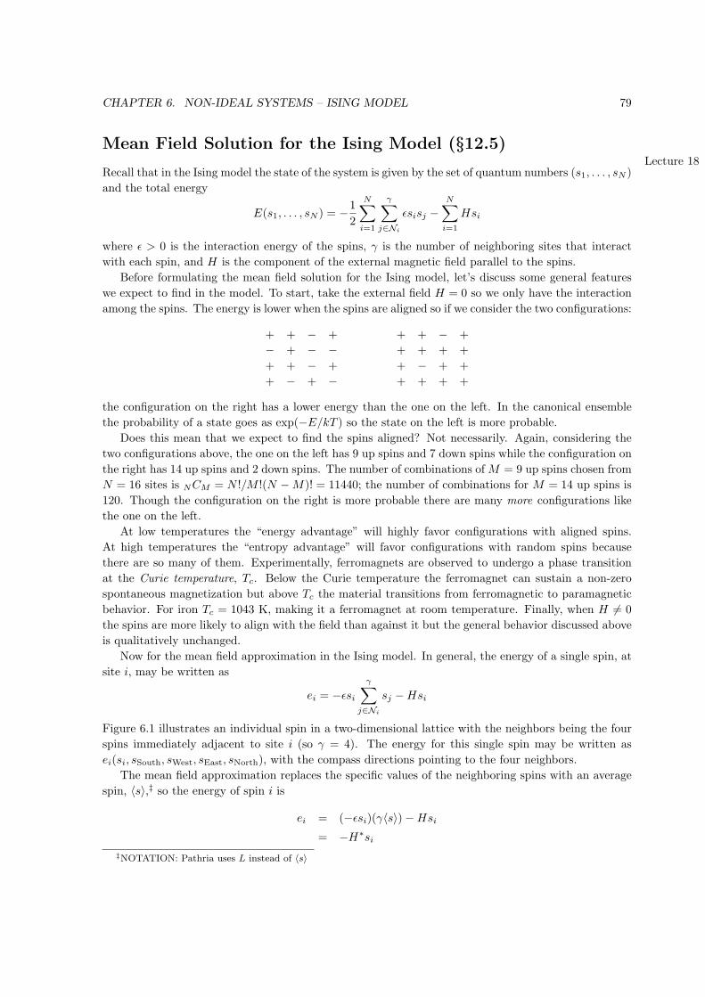
CHAPTER 6. NON-IDEAL SYSTEMS – ISING MODEL 79
Mean Field Solution for the Ising Model (§12.5)Lecture 18
Recall that in the Ising model the state of the system is given by the set of quantum numbers (s1, . . . , sN )
and the total energy
E(s1, . . . , sN ) = −1
2
N∑i=1
γ∑j∈Ni
ϵsisj −N∑i=1
Hsi
where ϵ > 0 is the interaction energy of the spins, γ is the number of neighboring sites that interact
with each spin, and H is the component of the external magnetic field parallel to the spins.
Before formulating the mean field solution for the Ising model, let’s discuss some general features
we expect to find in the model. To start, take the external field H = 0 so we only have the interaction
among the spins. The energy is lower when the spins are aligned so if we consider the two configurations:
+ + − +
− + − −+ + − +
+ − + −
+ + − +
+ + + +
+ − + +
+ + + +
the configuration on the right has a lower energy than the one on the left. In the canonical ensemble
the probability of a state goes as exp(−E/kT ) so the state on the left is more probable.
Does this mean that we expect to find the spins aligned? Not necessarily. Again, considering the
two configurations above, the one on the left has 9 up spins and 7 down spins while the configuration on
the right has 14 up spins and 2 down spins. The number of combinations of M = 9 up spins chosen from
N = 16 sites is NCM = N !/M !(N −M)! = 11440; the number of combinations for M = 14 up spins is
120. Though the configuration on the right is more probable there are many more configurations like
the one on the left.
At low temperatures the “energy advantage” will highly favor configurations with aligned spins.
At high temperatures the “entropy advantage” will favor configurations with random spins because
there are so many of them. Experimentally, ferromagnets are observed to undergo a phase transition
at the Curie temperature, Tc. Below the Curie temperature the ferromagnet can sustain a non-zero
spontaneous magnetization but above Tc the material transitions from ferromagnetic to paramagnetic
behavior. For iron Tc = 1043 K, making it a ferromagnet at room temperature. Finally, when H = 0
the spins are more likely to align with the field than against it but the general behavior discussed above
is qualitatively unchanged.
Now for the mean field approximation in the Ising model. In general, the energy of a single spin, at
site i, may be written as
ei = −ϵsi
γ∑j∈Ni
sj −Hsi
Figure 6.1 illustrates an individual spin in a two-dimensional lattice with the neighbors being the four
spins immediately adjacent to site i (so γ = 4). The energy for this single spin may be written as
ei(si, sSouth, sWest, sEast, sNorth), with the compass directions pointing to the four neighbors.
The mean field approximation replaces the specific values of the neighboring spins with an average
spin, ⟨s⟩,‡ so the energy of spin i is
ei = (−ϵsi)(γ⟨s⟩)−Hsi
= −H∗si
‡NOTATION: Pathria uses L instead of ⟨s⟩
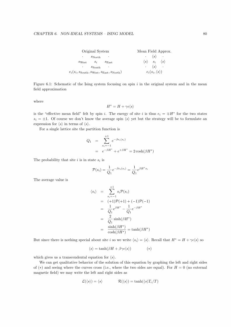
CHAPTER 6. NON-IDEAL SYSTEMS – ISING MODEL 80
Original System Mean Field Approx.
· sNorth ·sWest si sEast
· sSouth ·
· ⟨s⟩ ·⟨s⟩ si ⟨s⟩· ⟨s⟩ ·
ei(si, sSouth, sWest, sEast, sNorth) ei(si, ⟨s⟩)
Figure 6.1: Schematic of the Ising system focusing on spin i in the original system and in the mean
field approximation
where
H∗ = H + γϵ⟨s⟩
is the “effective mean field” felt by spin i. The energy of site i is thus ei = ∓H∗ for the two states
si = ±1. Of course we don’t know the average spin ⟨s⟩ yet but the strategy will be to formulate an
expression for ⟨s⟩ in terms of ⟨s⟩.For a single lattice site the partition function is
Q1 =
+1∑si=−1
e−βei(si)
= e−βH∗+ e+βH∗
= 2 cosh(βH∗)
The probability that site i is in state si is
P(si) =1
Q1e−βei(si) =
1
Q1eβH
∗si
The average value is
⟨si⟩ =+1∑
si=−1
siP(si)
= (+1)P(+1) + (−1)P(−1)
=1
Q1eβH
∗− 1
Q1e−βH∗
=2
Q1sinh(βH∗)
=sinh(βH∗)
cosh(βH∗)= tanh(βH∗)
But since there is nothing special about site i so we write ⟨si⟩ = ⟨s⟩. Recall that H∗ = H + γϵ⟨s⟩ so
⟨s⟩ = tanh(βH + βγϵ⟨s⟩) (∗)
which gives us a transcendental equation for ⟨s⟩.We can get qualitative behavior of the solution of this equation by graphing the left and right sides
of (∗) and seeing where the curves cross (i.e., where the two sides are equal). For H = 0 (no external
magnetic field) we may write the left and right sides as
L(⟨s⟩) = ⟨s⟩ R(⟨s⟩) = tanh(⟨s⟩Tc/T )
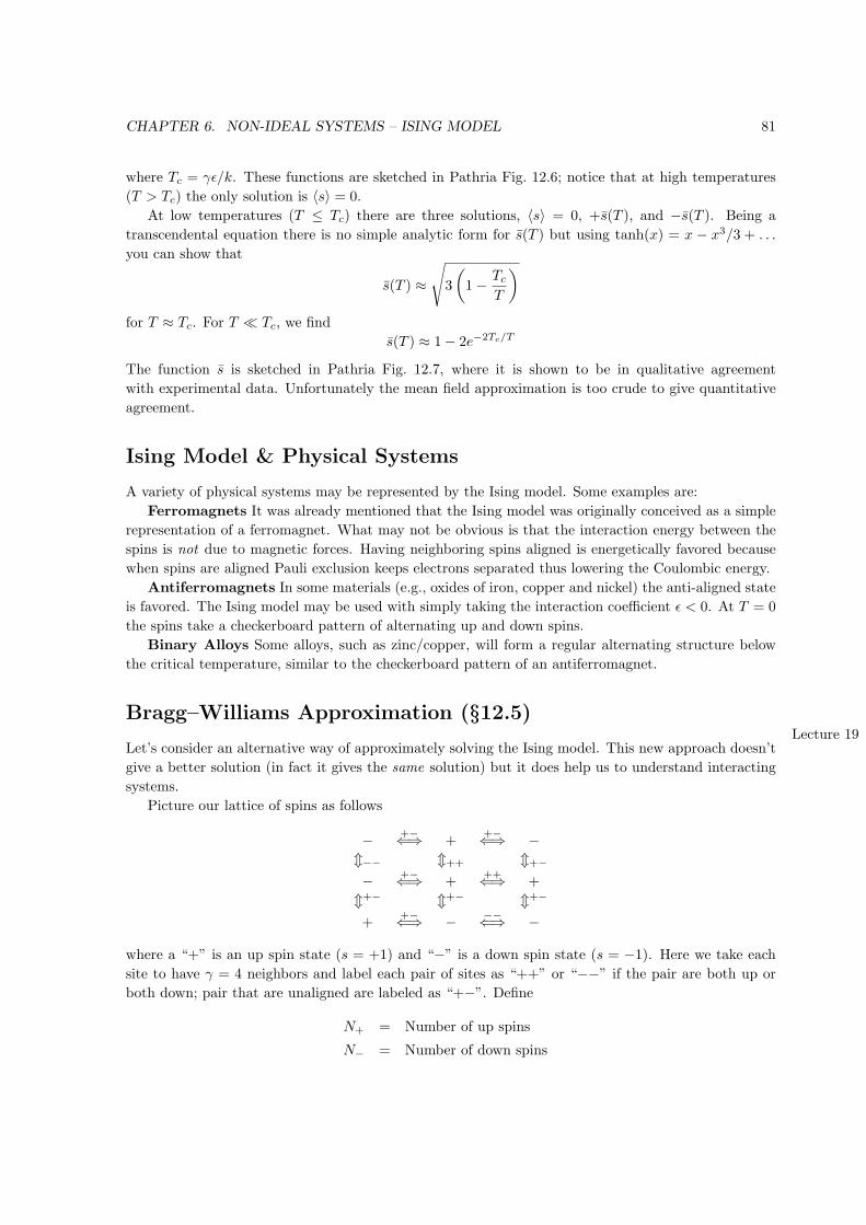
CHAPTER 6. NON-IDEAL SYSTEMS – ISING MODEL 81
where Tc = γϵ/k. These functions are sketched in Pathria Fig. 12.6; notice that at high temperatures
(T > Tc) the only solution is ⟨s⟩ = 0.
At low temperatures (T ≤ Tc) there are three solutions, ⟨s⟩ = 0, +s(T ), and −s(T ). Being a
transcendental equation there is no simple analytic form for s(T ) but using tanh(x) = x − x3/3 + . . .
you can show that
s(T ) ≈
√3
(1− Tc
T
)for T ≈ Tc. For T ≪ Tc, we find
s(T ) ≈ 1− 2e−2Tc/T
The function s is sketched in Pathria Fig. 12.7, where it is shown to be in qualitative agreement
with experimental data. Unfortunately the mean field approximation is too crude to give quantitative
agreement.
Ising Model & Physical Systems
A variety of physical systems may be represented by the Ising model. Some examples are:
Ferromagnets It was already mentioned that the Ising model was originally conceived as a simple
representation of a ferromagnet. What may not be obvious is that the interaction energy between the
spins is not due to magnetic forces. Having neighboring spins aligned is energetically favored because
when spins are aligned Pauli exclusion keeps electrons separated thus lowering the Coulombic energy.
Antiferromagnets In some materials (e.g., oxides of iron, copper and nickel) the anti-aligned state
is favored. The Ising model may be used with simply taking the interaction coefficient ϵ < 0. At T = 0
the spins take a checkerboard pattern of alternating up and down spins.
Binary Alloys Some alloys, such as zinc/copper, will form a regular alternating structure below
the critical temperature, similar to the checkerboard pattern of an antiferromagnet.
Bragg–Williams Approximation (§12.5)Lecture 19
Let’s consider an alternative way of approximately solving the Ising model. This new approach doesn’t
give a better solution (in fact it gives the same solution) but it does help us to understand interacting
systems.
Picture our lattice of spins as follows
− +−⇐⇒ ++−⇐⇒ −
−− ++ +−
− +−⇐⇒ +++⇐⇒ +
+− +− +−
++−⇐⇒ − −−⇐⇒ −
where a “+” is an up spin state (s = +1) and “−” is a down spin state (s = −1). Here we take each
site to have γ = 4 neighbors and label each pair of sites as “++” or “−−” if the pair are both up or
both down; pair that are unaligned are labeled as “+−”. Define
N+ = Number of up spins
N− = Number of down spins
CHAPTER 6. NON-IDEAL SYSTEMS – ISING MODEL 82
N++ = Number of up-up pairs
N−− = Number of up-down pairs
N+− = Number of up-down pairs
Since the total number of spins is N and the total number of pairs is 12γN ,
N+ +N− = N
N++ +N−− +N+− =1
2γN
Notice that the average value of the spin state may be written as
⟨s⟩ = 1
N
N∑i=1
si =N+ −N−
N
so
N+ =N
2(1 + ⟨s⟩)
N− =N
2(1− ⟨s⟩)
For ⟨s⟩ = 0, N+ = N− = N/2.
The total energy in the system may be written as
U = −1
2
N∑i=1
N∑j=1
sisjϵi,j −HN∑i=1
si
= −ϵ(N++ +N−− −N+−)−H(N+ −N−)
since the interaction coefficient ϵi,j = ϵ if spins i and j are neighbors and is zero otherwise.
So far we’ve made no approximations (and not gone very far). We now introduce the Bragg-William
approximation by assuming that
P++ = (P+)2
where P++ is the probability that a pair is “++” and P+ is the probability that a spin is up. This is
similar to the situation in which we flip a coin twice; the probability of getting two heads is the square
of the probability of getting a single head. Note that this is true even if it’s an unfair coin (i.e., change
of heads different from 50%).
Since
P+ =N+
N
P++ =N++12γN
the Bragg-William approximation may be written as
N++ =γ
2NN2
+
By a similar line of argument we also have
N−− =γ
2NN2
−
N+− =γ
NN+N−
CHAPTER 6. NON-IDEAL SYSTEMS – ISING MODEL 83
Putting all this into our energy expression gives
U = −ϵ(N++ +N−− −N+−)−H(N+ −N−)
= − ϵγ
2N(N2
+ +N2− − 2N+N−)−H(N+ −N−)
= − ϵγ
2N(N+ −N−)
2 −H(N+ −N−)
which may be written as
U(N+) = − ϵγ
2N(2N+ −N)2 −H(2N+ −N)
An alternative expression for the energy, using N+ = N2 (1 + ⟨s⟩), is
U(⟨s⟩) = −ϵγ
2N⟨s⟩2 −HN⟨s⟩ (∗)
Unfortunately, we still don’t know ⟨s⟩ so we’re not finished.
At this point we can use the microcanonical ensemble since we’ve formulated the energy as a function
of just N+. This means that the energy is fixed if N+ is fixed. But it is easy to count the total number
of states at fixed N+ since this is just the number of ways that we can pick N+ up spins from a set of
N , that is,
Γ(N+) =N !
N+!(N −N+)!=
N !
N+!N−!
In the microcanonical ensemble the entropy is
S = k ln Γ = k lnN !− k lnN+!− k lnN−!
Using lnM ! ≈ M lnM gives
S = kN lnN − kN+ lnN+ − kN− lnN−
which may be written as
S = −kN
2[(1 + ⟨s⟩) ln(1 + ⟨s⟩) + (1− ⟨s⟩) ln(1− ⟨s⟩)] (∗∗)
You can check that S → 0 as ⟨s⟩ → ±1.
We know the sort of behavior to expect: at high temperature the average spin is zero but below the
critical temperature the spins are favored to align. Since temperature is the key, let’s get an expression
for ⟨s⟩ in terms of T by evaluating
1
T=
(∂S
∂U
)H,N
=
(∂S∂⟨s⟩
)H,N(
∂⟨s⟩∂U
)H,N
Using (**) to evaluate the numerator and (*) to evaluate the denominator gives
1
T=
−kN2 ln
(1+⟨s⟩1+⟨s⟩
)−Nϵγ⟨s⟩+NH
=1
2ϵγ⟨s⟩+ 2Hln
(1 + ⟨s⟩1− ⟨s⟩
)
CHAPTER 6. NON-IDEAL SYSTEMS – ISING MODEL 84
We can do a bunch of algebra (but no further approximations) to arrive at the expression
⟨s⟩ = tanh(ϵγ⟨s⟩/kT +H/kT )
which is exactly the same transcendental equation we obtained from mean field theory. Naturally the
results obtained from mean field theory (e.g., critical temperature Tc = γϵ/k) are the same for the
Bragg-William approximation.
Finally, the reason that the mean field approximation and the Bragg-William approximation are
equivalent is that both represent the “long range order” in the Ising model but neglect the “short range
order.” In the real physical system, if a spin is up then it is more probable that a neighbor spin will also
be up; both approximations neglect this short-range correlation. If many spins are up then ⟨s⟩ will bepositive so in the mean field approximation the value of si will tend to be positive since spin i feels this
global field. In this sense the long-range correlation is included. For the Bragg-William approximation,
the number of “++” pairs (N++) depends only on the total number of up spins (N+) and not on how
they are distributed, which is equivalent to assuming the up spins are randomly distributed.
Any improvement of mean field theory will have to include short-range order. The simplest correc-
tion is called the Bethe approximation (section 12.6 in Pathria). Advanced methods are presented in
Chapters 13 and 14. The full story of the Ising model (and its variants) could easily occupy us for sev-
eral months. Instead of continuing its study we’ll move on to the general theory of critical phenomena.
But before leaving the Ising model, let’s consider one last important case which happens to be exactly
solvable.
One Dimensional Ising Chain (§13.2)We consider a system of N Ising spins arranged as a one-dimensional chain with nearest-neighbor
interactions, as pictured below+ − . . . + . . . −1 2 . . . i . . . N
In the absence of an external field (i.e., H = 0), the total energy is
E(s1, . . . , sN ) = −ϵ
N−1∑i=1
sisi+1
so the canonical partition function is
QN =+1∑
s1=−1
. . .+1∑
sN=−1
eβE
=+1∑
s1=−1
. . .+1∑
sN=−1
exp
(−ϵβ
N−1∑i=1
sisi+1
)
=
+1∑s1=−1
. . .
+1∑sN=−1
N−1∏i=1
exp(βϵsisi+1)
Using the identities
ex = cosh(x) + sinh(x)
cosh(−x) = cosh(x)
sinh(−x) = − sinh(x)

CHAPTER 6. NON-IDEAL SYSTEMS – ISING MODEL 85
and the fact that sisi+1 = ±1 gives
exp(βϵsisi+1) = cosh(βϵ) + sisi+1 sinh(βϵ) = (1 + sisi+1y) cosh(βϵ)
where y = tanh(βϵ).
The partition function is now
QN =+1∑
s1=−1
. . .+1∑
sN=−1
N−1∏i=1
(1 + sisi+1y) cosh(βϵ)
= coshN−1(βϵ)
+1∑s1=−1
. . .
+1∑sN=−1
N−1∏i=1
(1 + sisi+1y)
Let’s explicitly write out the product,
(1 + s1s2y)(1 + s2s3y) . . . (1 + sN−1sNy)
Doing the first sum,∑+1
s1=−1, makes the product
(1− s2y)[(1 + s2s3y) . . . (1 + sN−1sNy)] + (1 + s2y)[(1 + s2s3y) . . . (1 + sN−1sNy)]
or
2[(1 + s2s3y) . . . (1 + sN−1sNy)]
In fact, each time we do a sum we eliminate a term in the sum and pick up a factor of two.
The partition function for the one-dimensional Ising chain is just
QN = 2N coshN−1(βϵ)
Compare this with the partition function for non-interacting spins with energy levels of 0 and ϵ,
QN = (2 cosh(βϵ))N
which is the same as the 1D Ising partition function when N is large.
Interestingly, the 1D Ising chain has no critical point. Ising worked this out in writing his Ph.D.
thesis, published it in a short paper (his first) in 1925, became a high school teacher and never wrote
another paper! Though at the time he thought his model was a failure because of the negative result
he obtained for the one-dimensional case, to this day the Ising model is the topic of over 1000 papers a
year.
Chapter 7
Critical Phenomena
Universality in Critical PhenomenaLecture 20
We found that the average spin ⟨s⟩ (or total magnetic moment M ∝ N⟨s⟩) had the form of a “pitch-
fork” bifurcation. That is above the critical temperature ⟨s⟩ = 0 while below Tc we have non-zero
magnetization, as shown in Fig. 12.10 in Pathria and Beale. What is particularly interesting about this
result is that it appears to agree with all data for ferromagnetic materials (see Fig. 12.7 in Pathria and
Beale) at least when T ≈ Tc. This is surprising since different materials have different crystal structure,
material properties, etc. Furthermore, the Ising model is very simplistic.
These results suggest a universal behavior for systems near the critical point. For a specific material
the details of its structure and the nature of the interactions among its constituent atoms will affect
the value of Tc but the thermodynamic properties, when normalized by the values at the critical point,
will be universal.
Another example of this universality near the critical point is the liquid-vapor transition. Recall
the P − V diagram for the van der Waals model and the region of coexistence formulated using the
Maxwell construction (minimizing the Gibbs free energy). When the pressure, volume and temperature
are normalized by their values at the critical point then the experimental data for all materials fall on
the same curve, at least close to Tc (see Fig. 7.1) and have approximate quantitative agreement with van
der Waals. Given how difficult statistical mechanics can be for non-ideal systems, it seems worthwhile
to pursue these exceptional results.
Critical Exponents – A First Look (§12.2)To quantify how well mean field theory agrees with experiment (and with more advanced theories) we
define a set of power law exponents for the behavior of various thermodynamic quantities near the
critical point. To start, we define the critical exponent β as
⟨s⟩ ∝(Tc − T
Tc
)β
(T < Tc, T → Tc)
It’s not difficult to show that mean field theory gives
⟨s⟩ ∝√
Tc − T
Tc
86
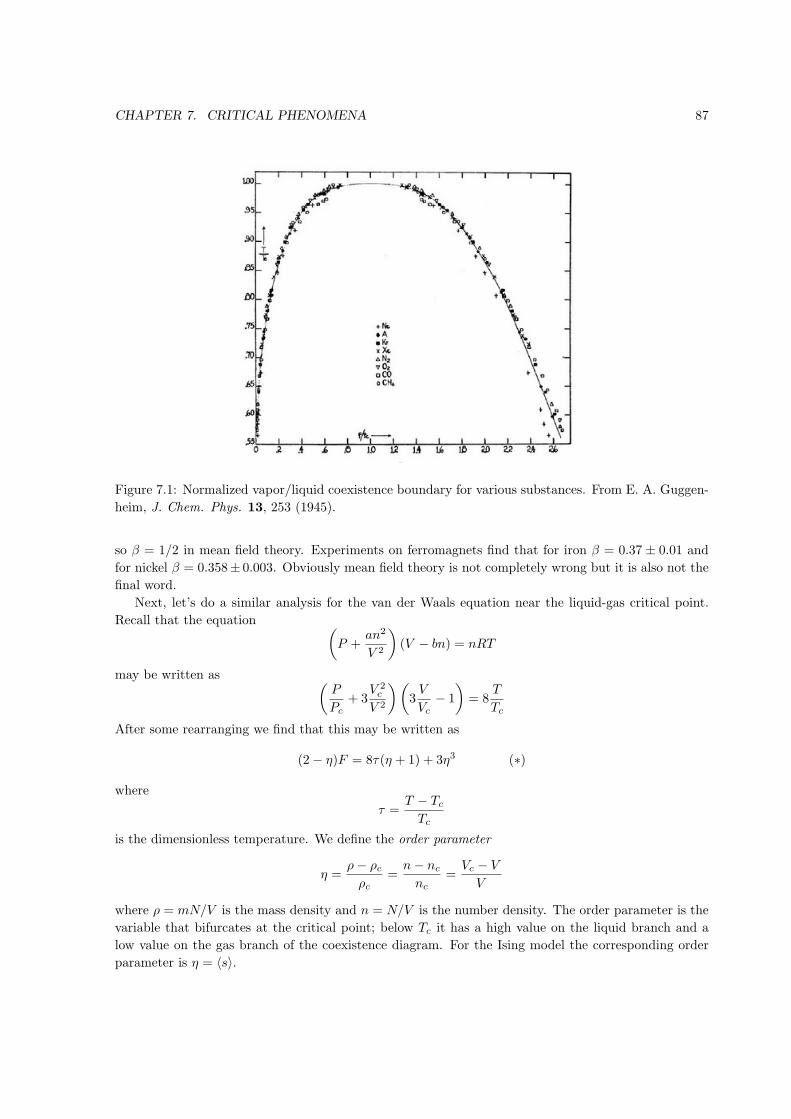
CHAPTER 7. CRITICAL PHENOMENA 87
Figure 7.1: Normalized vapor/liquid coexistence boundary for various substances. From E. A. Guggen-
heim, J. Chem. Phys. 13, 253 (1945).
so β = 1/2 in mean field theory. Experiments on ferromagnets find that for iron β = 0.37 ± 0.01 and
for nickel β = 0.358± 0.003. Obviously mean field theory is not completely wrong but it is also not the
final word.
Next, let’s do a similar analysis for the van der Waals equation near the liquid-gas critical point.
Recall that the equation (P +
an2
V 2
)(V − bn) = nRT
may be written as (P
Pc+ 3
V 2c
V 2
)(3V
Vc− 1
)= 8
T
Tc
After some rearranging we find that this may be written as
(2− η)F = 8τ(η + 1) + 3η3 (∗)
where
τ =T − Tc
Tc
is the dimensionless temperature. We define the order parameter
η =ρ− ρcρc
=n− nc
nc=
Vc − V
V
where ρ = mN/V is the mass density and n = N/V is the number density. The order parameter is the
variable that bifurcates at the critical point; below Tc it has a high value on the liquid branch and a
low value on the gas branch of the coexistence diagram. For the Ising model the corresponding order
parameter is η = ⟨s⟩.
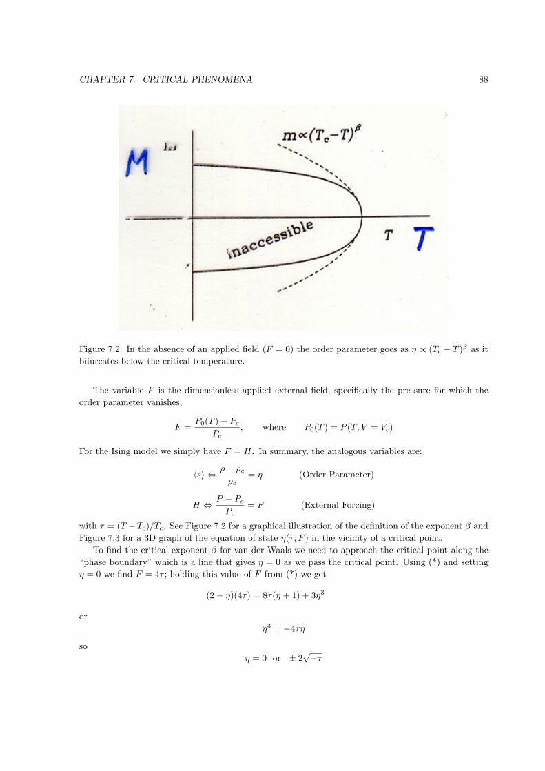
CHAPTER 7. CRITICAL PHENOMENA 88
Figure 7.2: In the absence of an applied field (F = 0) the order parameter goes as η ∝ (Tc − T )β as it
bifurcates below the critical temperature.
The variable F is the dimensionless applied external field, specifically the pressure for which the
order parameter vanishes,
F =P0(T )− Pc
Pc, where P0(T ) = P (T, V = Vc)
For the Ising model we simply have F = H. In summary, the analogous variables are:
⟨s⟩ ⇔ ρ− ρcρc
= η (Order Parameter)
H ⇔ P − Pc
Pc= F (External Forcing)
with τ = (T −Tc)/Tc. See Figure 7.2 for a graphical illustration of the definition of the exponent β and
Figure 7.3 for a 3D graph of the equation of state η(τ, F ) in the vicinity of a critical point.
To find the critical exponent β for van der Waals we need to approach the critical point along the
“phase boundary” which is a line that gives η = 0 as we pass the critical point. Using (*) and setting
η = 0 we find F = 4τ ; holding this value of F from (*) we get
(2− η)(4τ) = 8τ(η + 1) + 3η3
or
η3 = −4τη
so
η = 0 or ± 2√−τ

CHAPTER 7. CRITICAL PHENOMENA 89
Figure 7.3: Graph of the equation of state η(τ, F ) in the vicinity of a critical point (only the positive η
surface is shown).
CHAPTER 7. CRITICAL PHENOMENA 90
Above the critical temperature (τ > 0) the only solution is η = 0. But below Tc we have a pitchfork
bifurcation and the critical exponent is β = 1/2, just as we found with the Ising model. In fact, it turns
out that the van der Waals equation of state may be shown to arise from a mean field approximation
of the intermolecular attraction.
Landau Theory of Critical Phenomena
Given the results above and Maxwell’s formulation of the coexistence boundary based on minimizing the
Gibbs free energy, Landau suggested the following idea: The equilibrium state of a system is found by
minimizing the appropriate thermodynamic potential; for systems at constant temperature and pressure
that potential is the Gibbs free energy. Landau assumed that we may write the appropriate thermody-
namic potential as G(η, T ) and that above the critical temperature this potential has a single minimum
value, G0(T ) = G(0, T ) for T > Tc. Below the critical temperature there should be two minima and
Landau assumed that sufficiently close to the critical point those minima are symmetrically positioned
about η = 0. Finally, the function G(η, Tc) must have an inflection point to smoothly transition from
one minima to two minima as we pass the critical point. In brief, above Tc the thermodynamic potential
G(η, T ) is single-well and below Tc it is double-well with minima on each side of η = 0.
Since the order parameter is small near Tc, we can Taylor expand our thermodynamic potential as,
G(η, T ) = G0(T ) +1
2G2(T )η
2 +1
4G4(T )η
4 + . . .
where the odd terms are absent due to the assumption of symmetry. The simplest way to get the
desired transition of single-well to double-well is for G2(T ) to change sign from positive to negative as
the temperature drops below Tc. In the vicinity of the critical point we’ll assume that G(η, T ) has the
very simple form,
G(η, T ) = C0 +1
2C2τη2 +
1
4C4η4 + . . .
where C0, C2 and C4 are positive constants. Landau’s justification was that if the form of G(η, T ) isn’t
simple then the behavior won’t be universal.
To find the value of the order parameter at equilibrium we find the minima of G(η, T ); keeping only
the terms written above, (∂G
∂η
)T
= C2τη + C4η3 = 0
so
η = 0 or ±√
C2C4
√−τ
which, once again, produces a pitch-fork bifurcation of the order parameter as we pass through the
critical point with a critical exponent of β = 1/2.
Landau’s theory is the thermodynamic analog of mean field theory and it nicely ties together all
the results we’ve seen thus far. Unfortunately we only have approximate agreement with experimental
measurements so we don’t have a complete theory at this point.
More Critical Exponents
We already discussed one of the critical exponents, β, defined as,
η ∝ |τ |β
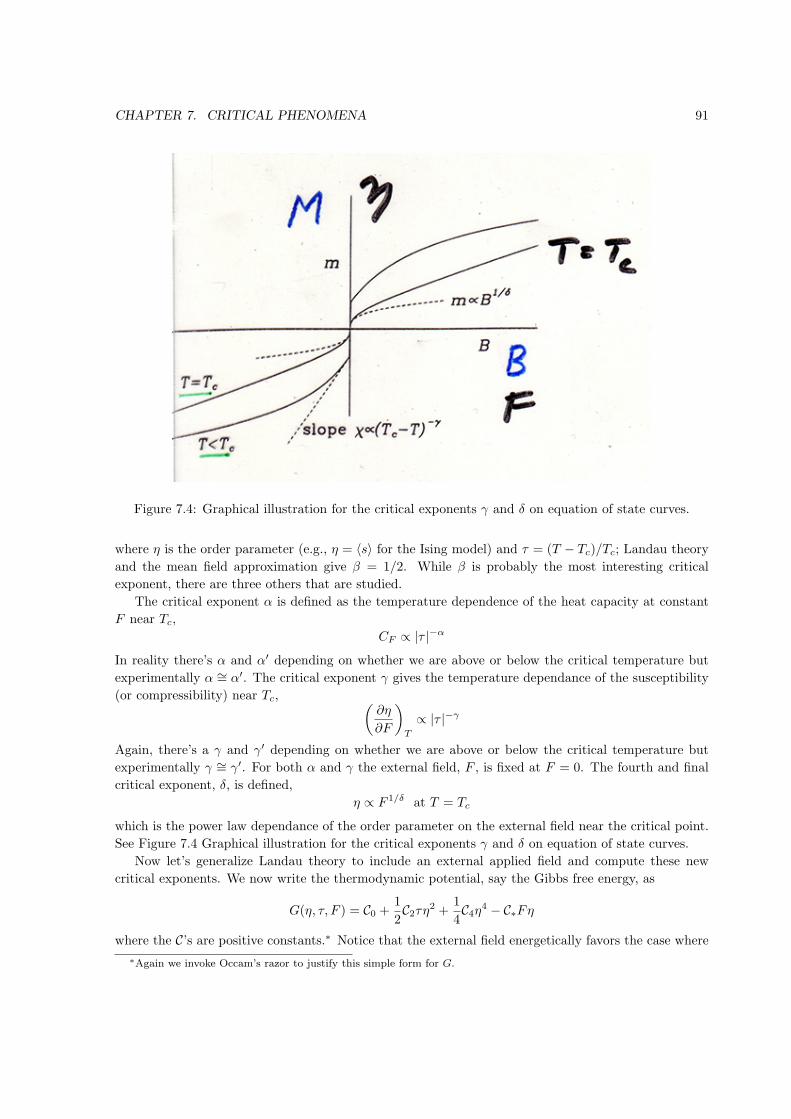
CHAPTER 7. CRITICAL PHENOMENA 91
Figure 7.4: Graphical illustration for the critical exponents γ and δ on equation of state curves.
where η is the order parameter (e.g., η = ⟨s⟩ for the Ising model) and τ = (T − Tc)/Tc; Landau theory
and the mean field approximation give β = 1/2. While β is probably the most interesting critical
exponent, there are three others that are studied.
The critical exponent α is defined as the temperature dependence of the heat capacity at constant
F near Tc,
CF ∝ |τ |−α
In reality there’s α and α′ depending on whether we are above or below the critical temperature but
experimentally α ∼= α′. The critical exponent γ gives the temperature dependance of the susceptibility
(or compressibility) near Tc, (∂η
∂F
)T
∝ |τ |−γ
Again, there’s a γ and γ′ depending on whether we are above or below the critical temperature but
experimentally γ ∼= γ′. For both α and γ the external field, F , is fixed at F = 0. The fourth and final
critical exponent, δ, is defined,
η ∝ F 1/δ at T = Tc
which is the power law dependance of the order parameter on the external field near the critical point.
See Figure 7.4 Graphical illustration for the critical exponents γ and δ on equation of state curves.
Now let’s generalize Landau theory to include an external applied field and compute these new
critical exponents. We now write the thermodynamic potential, say the Gibbs free energy, as
G(η, τ, F ) = C0 +1
2C2τη2 +
1
4C4η4 − C∗Fη
where the C’s are positive constants.∗ Notice that the external field energetically favors the case where
∗Again we invoke Occam’s razor to justify this simple form for G.
CHAPTER 7. CRITICAL PHENOMENA 92
F and η have the same sign. The order parameter at equilibrium is obtained by finding the minimum
of G so, as before, we evaluate(∂G
∂η
)τ,F
= C2τη + C4η3 − C∗F = 0 (∗)
We could solve this cubic but we don’t need the explicit solution for the purpose of finding the critical
exponents. The general shape of G is still either a single well or double well potential depending on
whether we are above or below the critical temperature; for F > 0 the largest positive root of this cubic
is the equilibrium state since it is the deeper well.
To evaluate the critical exponent γ we use (∗) to evaluate(∂F
∂η
)τ
=
(∂
∂η
)τ
[C2C∗
τη +C4C∗
η3]=
C2C∗
τ + 3C4C∗
η2
For T > Tc, F → 0, we know η → 0 (this is just the disordered state). From our earlier analysis we
also know that for T < Tc the order parameter η ∝ |τ |1/2 near the critical point. In summary, near the
critical point, (∂η
∂F
)τ
=
(
C2
C∗τ)−1
for T > Tc(C2
C∗τ + 3 C4
C∗|τ |)−1
for T < Tc
From the second law of thermodynamics we know that the isothermal susceptibility (or compressibility)
must be positive and so we find that both above and below the critical point,(∂η
∂F
)τ
∝ 1
|τ |
so γ = 1 in Landau theory.
Using (*) again but setting T = Tc (τ = 0) immediately gives
η =
(C∗C4
F
)1/3
so the critical exponent δ = 3 in Landau theory.
Finally, to get the exponent α we need to find the heat capacity; we’ll evaluate this using
CF = T
(∂S
∂T
)F
= −T
(∂2G
∂T 2
)F
= −1 + τ
Tc
(∂2G
∂τ2
)F
since dG = f(η)dF − SdT (e.g., for van der Waals dG = V dP − SdT ). Using our expression for G we
get, (∂2G
∂τ2
)F
= 2C2η(∂η
∂τ
)F
+ C2τ(∂η
∂τ
)2
F
+ C2τη(∂2η
∂τ2
)F
+3C4η2(∂η
∂τ
)2
F
+ C4η3(∂2η
∂τ2
)F
− C∗F(∂2η
∂τ2
)F
Since the critical exponent is defined at zero field (F = 0) the last term drops out. Above the critical
temperature η is constant (and equal to zero) so all the terms in the expression above are zero. Below
Tc we know that
η ∝ |τ |1/2 so
(∂η
∂τ
)F
∝ |τ |−1/2 ∝ 1
ηand
(∂2η
∂τ2
)F
∝ |τ |−3/2 ∝ 1
η3
CHAPTER 7. CRITICAL PHENOMENA 93
so we find that each term in (∂2G/∂τ2)F is constant so CF is a constant. Given the definition of α
being CF ∝ |τ |−α we have that α = 0 for Landau theory.
In summary, the Landau theory (and mean field theory) predict that the critical exponents are
α = 0 β = 1/2 γ = 1 δ = 3
Pathria and Beale list experimental data for a variety of physical systems (see Table 12.1) and find
values to be,
α = 0.0− 0.2 β = 0.30− 0.36 γ = 1.0− 1.4 δ = 4.0− 5.0
On the one hand the experimental values are comparable to the theoretical predictions and similar for
vastly different systems (magnets, gas-liquid mixtures, binary alloys, etc.). On the other hand, there
is some disagreement with theory and the values are similar among different systems but not entirely
universal.
Scaling Hypothesis §12.10By definition, a homogeneous function, f(x), has the property that
f(ax) = g(a)f(x)
where a is a constant. In fact, since this means that
f(abx) = g(ab)f(x) and f(abx) = g(a)g(b)f(x)
then g(a) must be a power law, that is,
f(ax) = arf(x)
We may write this result as
f(apx) = af(x)
where p = 1/r.
The scaling hypothesis assumes that the free energy (near Tc) is a homogeneous function of the
form,
G(apτ, aqF ) = aG(τ, F )
To obtain a relation between the coefficients p,q and the critical exponents, we apply the derivative to
both sides of this equation, (∂
∂F
)τ
G(apτ, aqF ) =
(∂
∂F
)τ
aG(τ, F )
Define the re-scaled values τ ′ = apτ and F ′ = aqF and we may write this equation as,[(∂
∂F ′
)τ
G(τ ′, F ′)
] [(∂F ′
∂F
)τ
]= a
(∂
∂F
)τ
G(τ, F )
Near the critical point the order parameter is proportional to the derivative of G with respect to the
external field, that is,
η ∝(∂G
∂F
)τ

CHAPTER 7. CRITICAL PHENOMENA 94
Using this observation we have,
η(τ ′, F ′)aq = aη(τ, F )
or
η(apτ, aqF ) = a1−qη(τ, F )
To grasp the meaning of this result, let’s consider a numerical example. It turns out that in Landau
theory p = 1/2 and q = 3/4. To get round numbers we’ll pick a = 16, so the result above gives,
η((16)(1/2)τ, (16)(3/4)F ) = (16)1/4η(τ, F )
or
η(4τ, 8F ) = 2η(τ, F )
That is, if we raise the temperature τ by a factor of 4 and also raise the applied field F by a factor of
8 then according to the scaling hypothesis the order parameter will double.
Now let’s directly link the scaling coefficients to the critical exponents. Suppose we take a =
(−τ)−1/p and set F = 0 so
η(((−τ)−1/p)pτ, 0) = ((−τ)−1/p)1−qη(τ, 0)
or
η(−1, 0) = ((−τ)−(1−q)/p)η(τ, 0)
The left hand side is a constant so
η(τ, 0) ∝ |τ |(1−q)/p thus β = (1− q)/p
Working along similar lines we can also derive that
α = 2− 1/p γ = (2q − 1)/p δ = q/(1− q)
These give two relations among the critical exponents so, for example, given β and γ we could find α
and δ. A simple form for the two relations is,
α+ 2β + γ = 2
α+ β(1 + δ) = 2
Recalling that the critical exponents in Landau theory are α = 0, β = 1/2, γ = 1, and δ = 3 we see
that they agree with this result from the scaling hypothesis. In fact these scaling hypothesis relations
appear to be exact. For example, for the Ising model in 2-dimensions can be solved exactly via a rather
long calculation (by Onsager) and one finds that,
α = 0 β = 1/8 γ = 7/4 δ = 15
which satisfy the two scaling hypothesis relations and give coefficients of p = 1/2 and q = 15/16.
Finally, the universality of the scaling hypothesis result has its origin in the long-ranged, self-similar
correlations that arise near a critical point, which is our last topic in the theory of critical phenomena.

CHAPTER 7. CRITICAL PHENOMENA 95
Critical Fluctuations §12.11, 12.12In describing thermodynamics systems we have taken them to be homogeneous. For the air in this
room we would assign an average number density, n, so the average number of particles in any given
(imaginary) volume is ⟨N⟩ = nV . Yet we know that the actual number of molecules in such a volume
would fluctuate, either if we looked at two different locations at the same time or looked in the same
location at two different times. † Typically the standard deviation of the fluctuations in N is a fraction
of the average value with
Standard Deviation
Average=
√⟨(N − ⟨N⟩)2⟩
⟨N⟩=
C√N
where the factor C =√nkTKT depends on the isothermal compressibility KT ; for an ideal gas C = 1.
In air at STP the number density is n = 2.7 × 1025m−3 so taking the volume as V = λ3Blue where
λBlue = 4.5×10⁻⁷ m is the wavelength of blue light we get about 2.5 million air molecules. The fractional
variation, 1/√
⟨N⟩, is a little less than a tenth of one percent; this is not enough to notice directly but
this variation in density (and the corresponding variation in the index of refraction) does produce
noticeable scattering of blue light over large distances, which is why the sky looks blue. Nevertheless
it’s a small effect so distant mountains have a bluish tint but not my face as viewed from across the
room.
At the critical point it’s a whole different ballgame. For example, for the liquid-vapor system the
isothermal compressibility goes as,
KT = − 1
V
(∂V
∂P
)T
∝ 1
|T − Tc|γ
where this critical exponent is γ ≈ 1.2 for water. At the critical point the compressibility diverges so it
takes no energy to expand or contract an element of fluid; the density undergoes wild fluctuations which
are macroscopically visible in a laboratory volume. Because these fluctuations turn the vapor mucky
the effect is known as critical opalescence; see www.youtube.com/watch?v=OgfxOl0eoJ0 for example.
Analogously, the isothermal susceptibility of a ferromagnet near the critical point goes as
χT ∝(∂⟨s⟩∂H
)∝ 1
|T − Tc|γ
where γ ≈ 1.3 for iron. From simulations of the Ising model we see that near the critical point we find
“islands” of all sizes, from single outcroppings to huge continents of aligned spins (with corresponding
“lakes” of the opposite alignment); see Figure 7.5. These structures at all sizes are analogous to the
density variations that create critical opalescence.
Correlations
To investigate these fluctuations near the critical point it makes sense to define a local order parameter,
η(r), such as the local number density at position r for liquid-vapor condensation. We define the
correlation function as,
g(r, r′) = ⟨η(r)η(r′)⟩ − ⟨η(r)⟩⟨η(r′)⟩†Assuming that the two locations or the two times were macroscopically distinct.
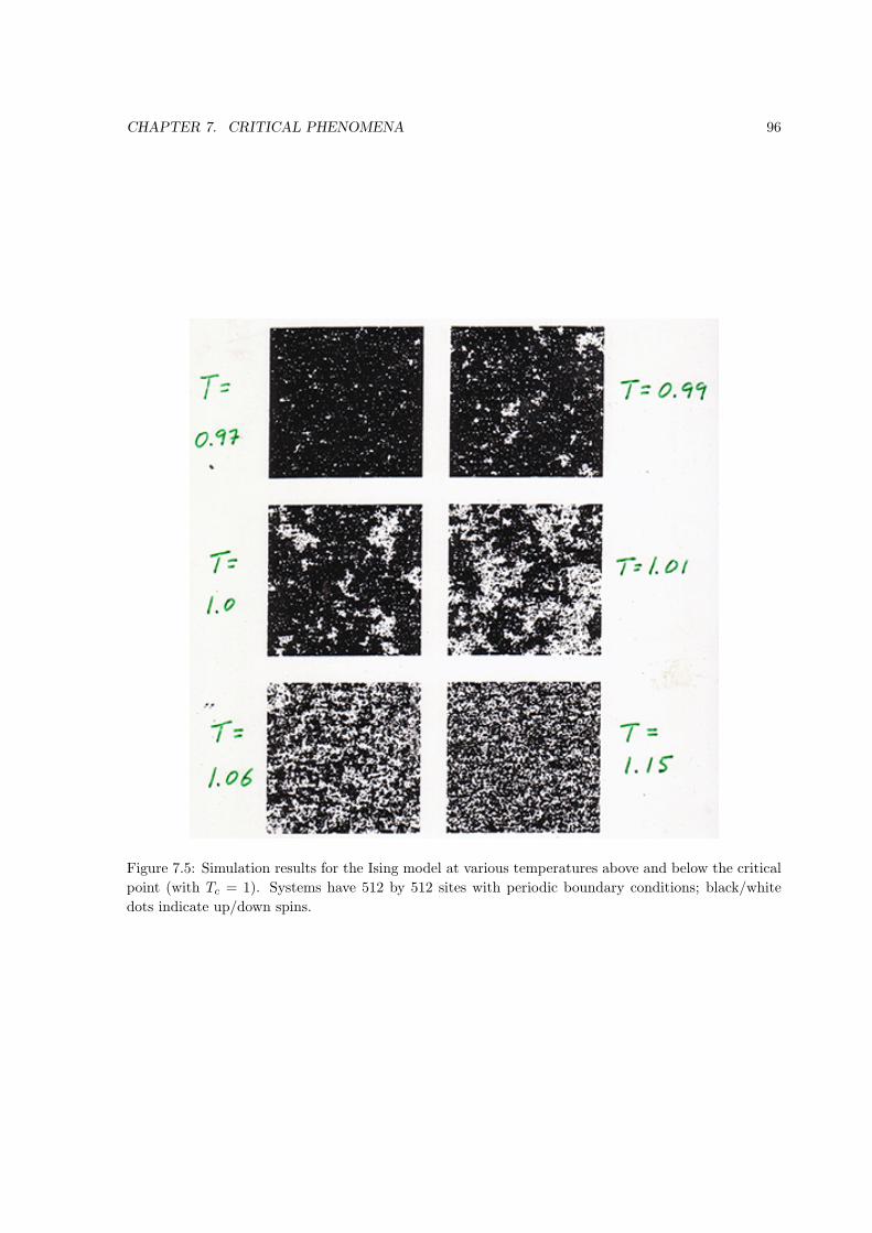
CHAPTER 7. CRITICAL PHENOMENA 96
Figure 7.5: Simulation results for the Ising model at various temperatures above and below the critical
point (with Tc = 1). Systems have 512 by 512 sites with periodic boundary conditions; black/white
dots indicate up/down spins.
CHAPTER 7. CRITICAL PHENOMENA 97
If η(r) and η(r′) are independent then g = 0. We can interpret this average as a time average, that is,
⟨f(η(r))⟩ = limt→∞
1
t
∫ t
0
f(η(r, t))dt
Since the order parameter is a mechanical variable (such as number of particles or number of up spins)
there’s no difficulty in defining the instantaneous value, η(r, t).‡
We still consider our equilibrium system to be statistically homogeneous (though not instantaneously
homogeneous) so we have ⟨η(r)⟩ = ⟨η(r′)⟩ and
g(r, r′) = g(|r − r′|) = g(∆r)
This correlation function is easy to measure in computer simulations and can be probed indirectly by
neutron scattering or light scattering in the laboratory. In both simulations and experiments one finds
that both above and below the critical point,
g(∆r) ∝ 1
∆re−∆r/ξ
for 3D systems. The correlation length, ξ, is not constant, in fact it increases and diverges as we
approach the critical point. Specifically,
ξ ∝ 1
|T − Tc|ν(T ≈ Tc)
The critical exponent, ν, is measured to be ν ≈ 0.5 − 0.8 (see Table 12.1 in Pathria and Beale). At
T = Tc the correlation function g(r) ∝ 1/r in 3D systems, so it is very long-ranged.
Ginzburg-Landau Theory
Let’s extend Landau theory to deal with spatial fluctuations of the order parameter. We now define
the local free energy density as,
G(r) = C0 +1
2C2τη(r)2 +
1
4C4η(r)4 − C∗F (r)η(r) +
1
2C∇(∇η)2
This should be familiar by now except for the last term, which depends on the spatial gradient of the
order parameter. This term accounts for the fact that although it is energetically favorable for the
system to be uniform (i.e., with zero gradients) and this term is constructed as the simplest possible
form that gives this behavior.
At equilibrium the total free energy,
GΣ =
∫drG(r)
is minimum; to find that minimum we want to evaluate
∂
∂ηGΣ =
∫dr [C2τη(r) + C4η(r)3 − C∗F (r) + C∇∇2η(r)]
‡Defining instantaneous values for non-mechanical variables, such as temperature, is a more delicate issue.

CHAPTER 7. CRITICAL PHENOMENA 98
where the last term comes from
∂
∂η
∫dr (∇η)2 =
∫dr 2(∇η)
∂
∂η(∇η)
= −2
∫dr (∇2η)
∂
∂ηη (Integration by parts)
= −2
∫dr ∇2η
and the last step is obtained using integration by parts. For the integral to vanish requires that
C′2τη(r) + C′
4η(r)3 − C′
∇∇2η(r) = F (r)
where C′2 = C2/C∗, etc.
Since we are interested in fluctuations we use perturbation theory and write,
η(r) = η0 + η1(r)
F (r) = F0 + F1(r)
where η0 = ⟨η(r)⟩ and F0 = ⟨F (r)⟩ are constants. Keeping only zero-th order terms we have
C′2τη0 + C′
4η30 = F0
which is our previous result for Landau theory (i.e., η0 is zero for T > Tc and has a pitchfork bifurcation
for T ≤ Tc). At first order in perturbation theory,
C′2τη1(r) + C′
4η20η1(r)− C′
∇∇2η(r) = F1(r)
or
(∇2 − ξ−2)η1(r) = − 1
C′∇F1(r)
which is the inhomogeneous Helmholtz equation with
ξ =
√C′∇
C′2τ + C′
4η20
Notice that for T > Tc we have η0 = 0 while for T < Tc we have η ∝√
|τ | so both above and below the
critical point we find
ξ ∝ 1
|τ |1/2In a moment we’ll see that this ξ is indeed the correlation length so Ginzburg-Landau theory predicts
the critical exponent ν = 1/2.
To finish the derivation, let’s pin the value of the order parameter at location r′ by setting f1(r) =
δ(r − r′). The solution to this Green’s function problem for the Helmholtz equation is (in 3D),
η1(r) ∝1
|r − r′|e−|r−r′|/ξ (Fixed η(r′))
This means that in the absence of an applied field the correlation function is
g(∆r) = ⟨η(r)η(r′)⟩ − ⟨η(r)⟩⟨η(r′)⟩= ⟨η1(r)η1(r′)⟩
∝ η1(r) ∝1
|r − r′|e−|r−r′|/ξ
where the last step is justified by the fact that the η1(r) gives the value of the order parameter for fixed
η(r′).
Chapter 8
Classical Non-ideal Gases
We now continue our study of systems with interacting particles (i.e., non-ideal) but in a new direction.
Up to now we’ve considered mainly the universal behavior that we find near the critical point. We now
turn to the more mundane problem of the specific behavior of specific systems, such as dense gases. The
advantage of studying the universal behavior was that since it was universal we could pick the simplest
systems, such as the Ising model, to study the behavior near the critical point. The disadvantage is
that we’re restricted to that small area of phase space.
In this chapter we’ll consider some basic approximations for treating dense gases, essentially finding
corrections to the ideal gas equation of state. We’ll also see how some of the ideas may be extended
to simple liquids. For the temperatures and pressures of interest the molecular interaction are well
approximated by classical potentials so we’ll restrict our attention to the classical canonical ensemble.
Pathria and Beale consider more advanced techniques, including some quantum mechanics calculations,
in their Chapter 10.
8.1 Canonical ensemble for non-ideal gases
Recall that in classical ensemble theory the state of a system of N particles is specified by the r1, . . . , rNpositions and p1, . . . , pN momenta, which marks a point in the 6N dimensional phase space. The
canonical partition function may be written as,
QN =1
N !h3N
∫dr1 . . .
∫drN
∫dp1 . . .
∫dpN exp−βE(r1, . . . , rN , p1, . . . , pN )
=1
N !h3N
∫dr1 . . .
∫drN exp−βV(r1, . . . , rN )
∫dp1 . . .
∫dpN exp−βK(p1, . . . , pN )
assuming that the total energy may be split as E = K + V where the kinetic energy, K, only depends
on the momenta and the potential energy, V, only depends on the positions of the particles. The 1/N !
factor accounts for the indistinguishability of the particles (recall Gibbs’ paradox) and the factor 1/h3N
is primarily for convenience, keeping the units consistent.
When we studied the classical ideal gas we assumed that U = 0 which is a good approximation when
the particles are far apart (i.e., dilute gas) since the inter-molecular potentials are very short ranged
(typically going like 1/r6). For the classical ideal gas we found,
QidealN =
V N
N !h3N
∫dp1 . . .
∫dpN exp−βK(p1, . . . , pN )
99
CHAPTER 8. CLASSICAL NON-IDEAL GASES 100
=1
N !h3N
(∫dp exp−β|p|2/2m
)N
=V N
N !λ3N
where λ = h/√2πmkT is the thermal wavelength. Using this result, we may write the partition function
for the non-ideal system as,
QN = QidealN
1
V N
∫dr1 . . .
∫drN exp−βV(r1, . . . , rN ) =
QidealN INV N
Note that for an ideal gas we have IN = V N .
To find the equation of state for this non-ideal system we could use,
P (T, V,N) = −(∂A
∂V
)T,N
=1
β
(∂
∂V
)T,N
lnQN
=1
β
(∂
∂V
)T,N
(lnQidealN + ln IN −N lnV )
=NkT
V− kT
[N
V−(
∂
∂V
)T,N
ln IN
]
= kT
(∂
∂V
)T,N
ln IN
Unfortunately the potential energy integral, IN , has a much more complex form, in general, than the
kinetic energy so we’ll have to make some approximations or limit ourselves to some simplified inter-
molecular potentials.
8.2 Hard Core Model
Suppose that the particles interact with a pure exclusion potential with no attraction and that the
volume occupied by each particle is v0. The simple physical picture to have in mind is that the particles
are hard spheres (e.g., tiny billiard balls). The potential energy for such a potential may be written as,
V(r1, . . . , rN ) =
0 no particles overlap
∞ otherwise
The probability of a point in phase space P(r1, . . . , rN ) is zero if any particles have positions that
overlap; all other points in phase space are equally probable. This might seem like it would be difficult
to work with but it turns out to be simple if we assume that the gas is not too dense.
Recall that we want to evaluate
IN =
∫dr1 . . .
∫drN exp−βV(r1, . . . , rN )
We can do the integral for the position of the first particle easily since it may be anywhere within the
volume so∫dr1 = V . The second particle may be anywhere within the volume except at positions where
it would overlap with the first particle. Since the particles have volume v0 we have∫dr2 = V − v0. For
the next particle we will assume that the system is not so dense that we have to worry about geometry
CHAPTER 8. CLASSICAL NON-IDEAL GASES 101
corrections that depend on the positions of the first two particles; in brief, we assume that the available
volume of phase space for the third particle is∫dr3 = V − 2v0.
Continuing in this way we find,
IN = (V )(V − v0)(V − 2v0) . . . (V − (N − 1)v0) =
N−1∏i=0
(V − iv0)
so
ln IN =
N−1∑i=0
ln(V − iv0)
To find the equation of state we evaluate,
P (T, V,N) = kT
(∂
∂V
)T,N
ln IN
= kTN−1∑i=0
1
V − iv0=
kT
V
N−1∑i=0
(1 + iv0/V )
=kT (N − 1)
V+ kT
v0V 2
(N − 1)(N − 2)
2
≈ NkT
V
(1 +
bN
V
)≈ NkT
V − bN
where b = v0/2. Notice that we get the van der Waals equation of state with only repulsion (i.e., van
der Waals attraction coefficient a = 0).
8.3 Intermolecular Potentials
The hard core model is obviously a highly simplified picture of intermolecular interactions. A more
accurate representation is to assume that the potential energy may be expressed in terms of pair-
potentials that only depend on the relative distance between particles, that is,
V(r1, . . . , rN ) =N∑i=1
N∑j=i+1
υ(|ri − rj |) ==1
2
N∑i=1
N∑j=1,j =i
υ(|ri − rj |)
This is a good approximation for simple molecules; far more complicated intermolecular models exist
but they’re mostly used in computer simulations.
Theory and measurement indicate that the potential υ(r) has two parts: a weak attraction term due
to dipole-dipole interactions and a strong but shorter-ranged repulsion due to Fermi exclusion of the
electron clouds. From E&M we know that the dipole-dipole potential goes as r−6 while the repulsion
term is not so short-ranged that it’s precise form is not too important so for convenience it’s usually
taken to be r−12. We’ll write this model potential, known as the Lennard-Jones potential, as,
υLJ(r) = 4ϵ
[(σr
)12−(σr
)6]where the parameter σ indicates the range of the potential and ϵ indicates the strength. See Figure 8.1
for a graph of the potential; note that the minimum of the potential well is at rmin = 21/6σ ≈ 1.12σ
and υLJ(rmin) = −ϵ.
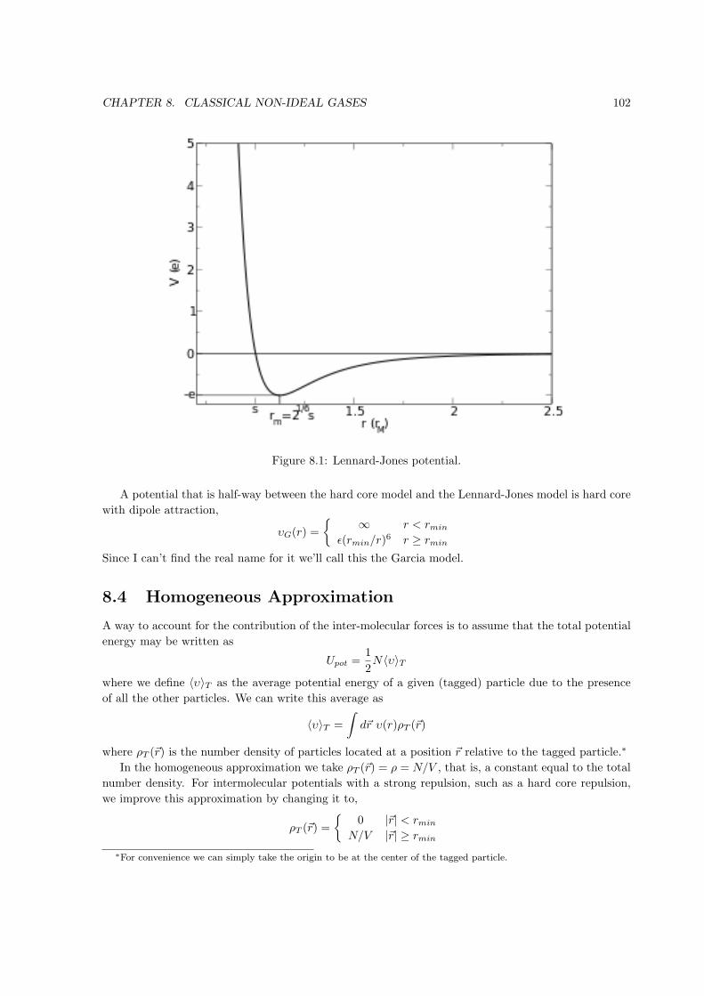
CHAPTER 8. CLASSICAL NON-IDEAL GASES 102
Figure 8.1: Lennard-Jones potential.
A potential that is half-way between the hard core model and the Lennard-Jones model is hard core
with dipole attraction,
υG(r) =
∞ r < rmin
ϵ(rmin/r)6 r ≥ rmin
Since I can’t find the real name for it we’ll call this the Garcia model.
8.4 Homogeneous Approximation
A way to account for the contribution of the inter-molecular forces is to assume that the total potential
energy may be written as
Upot =1
2N⟨υ⟩T
where we define ⟨υ⟩T as the average potential energy of a given (tagged) particle due to the presence
of all the other particles. We can write this average as
⟨υ⟩T =
∫dr υ(r)ρT (r)
where ρT (r) is the number density of particles located at a position r relative to the tagged particle.∗
In the homogeneous approximation we take ρT (r) = ρ = N/V , that is, a constant equal to the total
number density. For intermolecular potentials with a strong repulsion, such as a hard core repulsion,
we improve this approximation by changing it to,
ρT (r) =
0 |r| < rmin
N/V |r| ≥ rmin
∗For convenience we can simply take the origin to be at the center of the tagged particle.
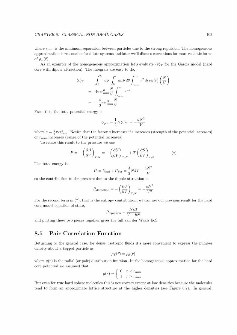
CHAPTER 8. CLASSICAL NON-IDEAL GASES 103
where rmin is the minimum separation between particles due to the strong repulsion. The homogeneous
approximation is reasonable for dilute systems and later we’ll discuss corrections for more realistic forms
of ρT (r).
As an example of the homogeneous approximation let’s evaluate ⟨υ⟩T for the Garcia model (hard
core with dipole attraction). The integrals are easy to do,
⟨υ⟩T =
∫ 2π
0
dϕ
∫ π
0
sin θ dθ
∫ ∞
rmin
r2 drυG(r)
(N
V
)= 4πϵr6min
N
V
∫ ∞
rmin
r−4
= −4
3πϵr3min
N
V
From this, the total potential energy is
Upot =1
2N⟨υ⟩T = −aN2
V
where a = 23πϵr
3min. Notice that the factor a increases if ϵ increases (strength of the potential increases)
or rmin increases (range of the potential increases).
To relate this result to the pressure we use
P = −(∂A
∂V
)T,N
= −(∂U
∂V
)T,N
+ T
(∂S
∂V
)T,N
(∗)
The total energy is
U = Ukin + Upot =3
2NkT − aN2
V
so the contribution to the pressure due to the dipole attraction is
Pattraction = −(∂U
∂V
)T,N
= −aN2
V 2
For the second term in (*), that is the entropy contribution, we can use our previous result for the hard
core model equation of state,
Prepulsion =NkT
V − bN
and putting these two pieces together gives the full van der Waals EoS.
8.5 Pair Correlation Function
Returning to the general case, for dense, isotropic fluids it’s more convenient to express the number
density about a tagged particle as
ρT (r) = ρg(r)
where g(r) is the radial (or pair) distribution function. In the homogeneous approximation for the hard
core potential we assumed that
g(r) =
0 r < rmin
1 r > rmin
But even for true hard sphere molecules this is not correct except at low densities because the molecules
tend to form an approximate lattice structure at the higher densities (see Figure 8.2). In general,
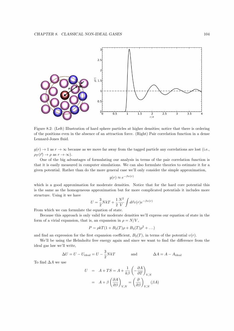
CHAPTER 8. CLASSICAL NON-IDEAL GASES 104
Figure 8.2: (Left) Illustration of hard sphere particles at higher densities; notice that there is ordering
of the positions even in the absence of an attraction force. (Right) Pair correlation function in a dense
Lennard-Jones fluid.
g(r) → 1 as r → ∞ because as we move far away from the tagged particle any correlations are lost (i.e.,
ρT (r) → ρ as r → ∞).
One of the big advantages of formulating our analysis in terms of the pair correlation function is
that it is easily measured in computer simulations. We can also formulate theories to estimate it for a
given potential. Rather than do the more general case we’ll only consider the simple approximation,
g(r) ≈ e−βυ(r)
which is a good approximation for moderate densities. Notice that for the hard core potential this
is the same as the homogeneous approximation but for more complicated potentials it includes more
structure. Using it we have
U =3
2NkT +
1
2
N2
V
∫drυ(r)e−βυ(r)
From which we can formulate the equation of state.
Because this approach is only valid for moderate densities we’ll express our equation of state in the
form of a virial expansion, that is, an expansion in ρ = N/V ,
P = ρkT (1 +B2(T )ρ+B3(T )ρ2 + . . .)
and find an expression for the first expansion coefficient, B2(T ), in terms of the potential υ(r).
We’ll be using the Helmholtz free energy again and since we want to find the difference from the
ideal gas law we’ll write,
∆U = U − Uideal = U − 3
2NkT and ∆A = A−Aideal
To find ∆A we use
U = A+ TS = A+1
kβ
(−∂A
∂T
)V,N
= A+ β
(∂A
∂β
)V,N
=
(∂
∂β
)V,N
(βA)
CHAPTER 8. CLASSICAL NON-IDEAL GASES 105
so
∆U =
(∂
∂β
)V,N
(β∆A)
This is useful once you notice that,
∆U =1
2
N2
V
∫drυ(r)e−βυ(r)
= −(
∂
∂β
)V,N
1
2
N2
V
∫dre−βυ(r)
so by comparing the two expression above for ∆U we have,
β∆A = −1
2
N2
V
∫dr[e−βυ(r) + C
]where C is a constant of integration; we know that C = −1 since ∆A = 0 if υ(r) = 0 (ideal gas limit).
We can now get the deviation from the ideal gas pressure, ∆p, from
∆P = −(
∂
∂V
)T,N
∆A = −1
2
N2
V 2
∫dr[e−βυ(r) − 1
]so
P = Pideal +∆P = ρkT
(1− 1
2ρ
∫dr[e−βυ(r) − 1
])Comparing with the virial expansion we see that
B2(T ) = −1
2
∫dr[e−βυ(r) − 1
]= −1
2
∫drf(r)
where f(r) = e−βυ(r) − 1 is known as the Mayer function.
Chapter 9
Fluctuations and Stochastic
Processes
Thermodynamic Fluctuations (14.1)Lecture xx
A system at thermodynamic equilibrium is extremely homogeneous. Most fluctuations we observe in
daily phenomena (e.g., dust particles dancing in the air, density ripples of air above hot asphalt) are non-
equilibrium phenomena. Though equilibrium fluctuations are typically extremely small in magnitude
they are fundamentally important (and sometimes have important effects).
Recall that in the micro-canonical ensemble a system with fixed energy U and volume V is at
equilibrium when its entropy, S(U, V ), is maximum. Let’s take such a system and split it into two parts
(UΣ = U1 +U2, VΣ = V1 +V2, NΣ = N1 +N2) The first being much smaller than the second (U1 ≪ U2,
V1 ≪ V2, N1 ≪ N2); for simplicity take N1, N2 fixed.
Call T ∗ and P ∗ the temperature and pressure at equilibrium. The average temperature of each part
is T 1 = T 2 = T ∗, similarly for pressure.
We ask the following question: “Suppose that we measure T1 at random, what is the probability
of a fluctuation ∆T1 = T1 − T ∗?” This is the formal version of the question, “What’s the chance that
water will spontaneously boil in the corner of your glass of water?”
Call S∗Σ the entropy at equilibrium, that is,
S∗Σ = S1(U1, V 1) + S2(U2, V 2) = S1 + S2
For different values the system has a lower entropy, that is,
SΣ = S1(U1, V1) + S2(U2, V2) ≤ S0
The probability of this fluctuation, P(S), may be found by using
S = k ln Γ
where Γ is the number of accessible states for the system. Specifically,
P(S) ∝ Γ
Γ0=
eSΣ/k
eS∗Σ/k
= e(SΣ−S∗Σ)/k = e∆SΣ/k
We’ll be OK without having to find the normalization so don’t worry that the above is “goes as” rather
than ”equals.”
106
CHAPTER 9. FLUCTUATIONS AND STOCHASTIC PROCESSES 107
Now we want to analyze ∆SΣ in terms of the states of parts 1 and 2 of the system; specifically,
∆SΣ = SΣ − SΣ = (S1 − S1) + (S2 − S2) = ∆S1 +∆S2
Since the fluctuations are small we can use the differential version of the first and second laws
∆U2 = T2∆S2 − P2∆V2
or
∆S2 =1
T2(∆U2 + P2∆V2)
There’s a similar expression for ∆S1 but we won’t need it.
Can now write
∆SΣ = ∆S1 +1
T2(∆U2 + P2∆V2)
and make the following two observations: 1) Since U = U1 + U2 is fixed, ∆U2 = −∆U1 and similarly
∆V2 = −∆V1. 2) Since system 2 is very large T2 ≈ T ∗ and P2 ≈ P ∗ (i.e., fluctuations only have a
significant effect in the smaller part). From these observations,
∆SΣ = ∆S1 −1
T ∗∆U1 −P ∗
T ∗∆V1 (∗)
We now have ∆S in terms of fluctuations in system 1; the next step is to replace ∆U1 with an expression
involving only temperature, pressure, etc.
We now write U1(S1, V1) and Taylor expand it about the equilibrium state,
U1(S1, V1) = U1(S1, V 1) +
(∂U1
∂S1
)V
∆S1 +
(∂U1
∂V1
)S
∆V1
+1
2
[(∂2U1
∂S21
)V
(∆S1)2 +
(∂2U1
∂S1∂V1
)(∆S1)(∆V1) +
(∂2U1
∂V 21
)S
(∆V1)2
]+ . . .
where the overbar indicates that the quantity is evaluated at equilibrium. For example,(∂U1
∂S1
)V
= T ∗(∂U1
∂V1
)S
= −P ∗
To deal with the quadratic term in the square brace, use the Taylor expansion
T1 =
(∂U1
∂S1
)V
=
(∂U1
∂S1
)V
+
(∂2U1
∂S21
)V
∆S1 +
(∂2U1
∂V1∂S1
)∆V1 + . . .
and note that the first term on the r.h.s. equals T ∗ so
∆T1 = T1 − T ∗ =
(∂2U1
∂S21
)V
∆S1 +
(∂2U1
∂V1∂S1
)S
∆V1
and so multiplying both sides by ∆S1 gives,
(∆T1)(∆S1) =
(∂2U1
∂S21
)V
(∆S1)2 +
(∂2U1
∂V1∂S1
)(∆S1)(∆V1)
By a similar line of reasoning, we obtain
−(∆P1)(∆V1) =
(∂2U1
∂V 21
)S
(∆V1)2 +
(∂2U1
∂V1∂S1
)(∆S1)(∆V1)

CHAPTER 9. FLUCTUATIONS AND STOCHASTIC PROCESSES 108
Collecting the above,
U1(S1, V1) = U1(S1, V 1) + T ∗∆S1 − P ∗∆V1
+1
2[(∆T1)(∆S1)− (∆P1)(∆V1)]
and putting this into (*) gives, ∗
∆S = ∆S1 −P ∗
T ∗∆V1 −1
T ∗
T ∗∆S1 − P ∗∆V1
+1
2[(∆T1)(∆S1)− (∆P1)(∆V1)]
= − 1
2T ∗ [(∆T1)(∆S1)− (∆P1)(∆V1)]
We have one more step but before we finish let’s simplify the notation and write this expression as just,
∆SΣ = − 1
2T[(∆T )(∆S)− (∆P )(∆V )]
so implicitly all the quantities are for system 1 and evaluated at equilibrium, that is, we’ll simply write
T instead of T ∗ for intensive variables and V instead of V 1 for extensive variables.
We are almost finished but our expression for ∆SΣ needs one last manipulation since the four vari-
ables ∆T,∆S,∆P and ∆V are not independent. Let’s take ∆T and ∆V as the independent variables;
to replace ∆S and ∆P we use,
∆S =
(∂S
∂T
)V
∆T +
(∂S
∂V
)T
∆V =Cv
T∆T +
(∂P
∂T
)V
∆V
∆P =
(∂P
∂T
)V
∆T +
(∂P
∂V
)T
∆V =
(∂P
∂T
)V
∆V − 1
V KT∆V
Finally, the probability of a fluctuation in temperature and volume is,
P(∆T,∆V ) = P(∆SΣ) ∝ exp
− Cv
2kT 2(∆T )2 − 1
2kTKTV(∆V )2
= exp(−(∆T )2/2σ2
T ) exp(−(∆V )2/2σ2V )
We see that P(∆T,∆V ) factors into a pair of Gaussian distributions† of the form,
P(x) = Ae−x2/2σ2
(Gaussian distribution)
where A is the normalization constant and σ is the standard deviation In this form for the Gaussian
the mean, x = 0, and the variance (x− x)2 = x2 = σ2 so,
∆T 2 =kT 2
Cv∆V 2 = kTKTV
Finally, since the distribution factors into a pair of distributions for ∆T and ∆V that means that these
variables are independent (i.e., uncorrelated) so ∆T∆V . By the way, this result for the variances in
∗You see why we kept N fixed for simplicity; as an exercise repeat this analysis to find ∆SΣ with U , V , and N as
variables.†Also known as the normal distribution.
CHAPTER 9. FLUCTUATIONS AND STOCHASTIC PROCESSES 109
temperature and volume is unchanged if we allow N to vary as well. Pathria and Beale discuss the
variances for other variables, such as ∆S2, ∆P 2, etc.
Let’s finish by putting in some values into these expressions to get a sense of the magnitude of the
fluctuations. For a Gaussian distribution the probability that a random value is 3σ above the mean is
about 0.2% and the probability that it is 9σ above the mean is about 10−19. The heat capacity of one
milliliter‡ of water at room temperature is about 4 Joules per Kelvin so for temperature fluctuations,
σT =√∆T 2 =
√kT 2
Cv≈ 5× 10⁻¹⁰ Kelvin
Even if you’ve been watching that glass of water since the start of the Universe (about 1018 seconds)
you’re not going to see a corner start to spontaneously boil (or even get noticeable warm). This result
isn’t surprising since, in general, the ratio of the fluctuation to the mean values go as 1/√N so for
macroscopic volumes where N is on the order of Avogadro’s number these deviations are negligible.
On the other hand, at microscopic scales they are significant. Consider a yoctoliter§ of water at
room temperature; for this volume the standard deviation of temperature fluctuations is,
σT ≈ (5× 10⁻¹⁰ Kelvin)×√
10−6
10−27≈ 15 Kelvin
This microscopic volume has roughly a hundred water molecules so the fluctuations in temperature are
noticeable.
Brownian MotionLecture xx
We now analyze a specific phenomenon connect to spontaneous thermal fluctuations. Consider a small
particle, such a pollen grain, that is neutrally buoyant in water. The grain is much larger than a
molecule of water so it is visible under a microscope. But it is also small enough that the random
impacts of the water molecules cause noticeable effects. We’ll refer to such a particle as a Brownian
particle.
Consider a particle with a radius of 1 micron (which is about twice the wavelength of visible light)
and a density of 1 g/cm3 (about the density of wood and of water); its mass is about 4 × 10⁻¹⁵ kg.
From the equipartition theorem we expect the mean kinetic energy of the Brownian particle is given by,
⟨ 12mv2⟩ = 32kT
so the r.m.s. speed of the particle is, √⟨v2⟩ =
√3kT/m
For T = 300 K we find that the particle’s speed is almost 2 millimeters per second. If it traveled
ballistically then in one second it would fly a distance of about 2000 radii; under the microscope it
would look like a blur. But due to the constant collisions with the water molecules the direction and
magnitude of the Brownian particle’s velocity changes randomly.¶
‡One milliliter equals one cubic centimeter equals 10−6 m3.§One yoctoliter equals one cubic nanometer equals 10−27 m3.¶The ratio of the r.m.s. momentum of the Brownian particle compared with a water molecule equals the square root
of the ratio of their masses.
CHAPTER 9. FLUCTUATIONS AND STOCHASTIC PROCESSES 110
Random Walk Model
Consider the following cartoon for the motion of the Brownian particle. For simplicity we’ll restrict the
motion to one-dimensional motion along the x-axis with the particle starting at x = 0 at t = 0; the
generalization to 3D motion will be straight-forward. To further simplify the formulation we’ll assume
that at integer time steps the particle moves a unit distance with equal probability of going to the left
or to the right. This is called the random walk model.∥ Notice that if the particle moved ballistically
(e.g., all steps were to the right) then the particle would have unit speed.
At time t = n the particle has taken n steps with n+ steps to the right and n− = n − n+ steps to
the left. The probability of taking n+ steps to the right is
Pn(n+) =
(1
2
)nn!
n+!(n− n+)!
The problem is similar to finding the probability of getting exactly n+ “heads” when flipping a fair coin
n times. Note that we could do the more general case where the probability of taking a step to the
right is p+ and to the left is p− = (1− p+) for which we’d have,
Pn(n+) = pn+
+ (1− p+)n−n+
n!
n+!(n− n+)!
But for simplicity we’ll stay with the symmetric case where p+ = 1/2.
The position of the particle is m = n+ − n− = 2n+ − n so the probability of the particle being at
position m is
Pn(m) =
(1
2
)n((n+m)/2)!
((n−m)/2)!
We can now compute a few average quantities, starting with the average position,
⟨m⟩ =n∑
m=−n
mPn(m)
For this calculation it will actually be easier to work with n+ instead of m and convert using
⟨m⟩ = 2⟨n+⟩ − n
Remember that since taking an average is a linear operation (either summing or integrating over possible
values) we have, in general,
⟨af(x) + bg(x)⟩ = a⟨f(x)⟩+ b⟨g(x)⟩
where the average is over the probability P(x).
To find ⟨n+⟩ we use the binomial expansion,
(p+ q)n =n∑
n+=0
pn+qn−n+n!
n+!(n− n+)!= qn + npqn−1 + . . .+ npn−1q + pn
We now use a common trick in manipulating these types of series and differentiate both sides,
d
dp(p+ q)n =
d
dp
n∑n+=0
pn+qn−n+n!
n+!(n− n+)!
∥The historical, less politically correct name is the “drunkard’s walk” model.
CHAPTER 9. FLUCTUATIONS AND STOCHASTIC PROCESSES 111
so
n(p+ q)n−1 =n∑
n+=0
n+pn+−1qn−n+
n!
n+!(n− n+)!
Now if we set p = q = 1/2 in this expression,
n =
n∑n+=0
n+
(1
2
)n
− 1n!
n+!(n− n+)!= 2
n∑n+=0
n+Pn(n+)
so
⟨n+⟩ =n∑
n+=0
n+Pn(n+) =n
2
which is not surprising since, on average, we take n/2 steps to the right and n/2 steps to the left. From
this result we directly find that ⟨m⟩ = 0, which is also no surprise.
The more interesting result comes from repeating the differentiation trick again, which after a little
algebra gives ⟨n2+⟩ = n(n+ 1)/4 so
⟨m2⟩ = ⟨(2n+ − n)2⟩ = 4⟨n2+⟩ − 4n⟨n+⟩+ n2 = n
The r.m.s. displacement of the particle is√⟨m2⟩ =
√n; contrast this with the ballistic displacement
(distance traveled if all the steps were in the same direction), which is n.
Simple Diffusion
To make a closer connection between the random walk model and the diffusive, random motion of
a Brownian particle we’ll formulate the probability distribution Pn(m) in the limit where n is large.
Naturally, the first step is to use Sterling’s approximation for the factorials,
lnn! ≈ n lnn− n+1
2ln 2πn
Note that we’re using one more term than usual. Recalling our earlier result,
lnPn(m) = −n ln 2 + lnn!− ln(12 (n+m)!)− ln(12 (n−m)!)
≈ n lnn− 12 (n+m) ln(n+m)− 1
2 (n−m) ln(n−m) + 12 ln 2πn− 1
2 ln(π2(n2 −m2))
= n lnn− 12n ln(n2 −m2)− 1
2m lnn+m
n−m+ 1
2 ln2n
π(n2 −m2)
Next we’ll take the limit of n ≫ m, which is reasonable since we know that√⟨m2⟩ =
√n so the
probability Pn(m) drops off rapidly with increasing |m|. This allows us to write,
lnPn(m) = n lnn− 12n ln
[n2(1−m2/n2)
]− 1
2m ln(1 +m/n)2
]+ 1
2 ln(2/πn)
= − 12n ln
[1− m2
n2
]−m ln(1 +m/n) + 1
2 ln(2/πn)
Finally, using ln(1 + x) ≈ x for x ≪ 1 gives,
lnPn(m) ≈ 1
2
m2
n− m2
n+
1
2ln(2/πn)

CHAPTER 9. FLUCTUATIONS AND STOCHASTIC PROCESSES 112
or
Pn(m) ∝√
1
ne−m2/2n
Not surprisingly, after all those approximations we have to multiply by the appropriate constant to
normalize the distribution.∗∗ Doing so yields,
Pn(m) =
√1
2πne−m2/2n
which is a Gaussian distribution with mean ⟨m⟩ = 0 and variance ⟨(m− ⟨m⟩)2⟩ = ⟨m2⟩ =√n.
Passing from discrete to continuous space (m → x) and from discrete steps to continuous time
(n → t) we obtain,
P(x, t) =
√1
4πDte−x2/4Dt (∗)
where D is the diffusion coefficient. This coefficient is implicit in the assumption in the random walk
model that the steps are unit length and occur at unit times. The mean and variance of this distribution
are,
⟨x⟩ =
∫ ∞
−∞dxxP(x, t) = 0
⟨(x− ⟨x⟩)2⟩ =
∫ ∞
−∞dx (x− ⟨x⟩)2P(x, t) = 2Dt
so the r.m.s. displacement is√⟨(x− ⟨x⟩)2⟩ =
√⟨x2⟩ =
√2Dt.
You may already be familiar with the fact that this Gaussian function (*) is the solution of the
diffusion equation,∂
∂tP(x, t) = D
∂2
∂x2P(x, t)
for the initial condition,
P(x, t) = δ(x)
and no boundary conditions (i.e., x extends from −∞ to ∞). From inspection of (*) the amplitude of
P(x, t) at x = 0 diverges for t = 0 while the standard deviation goes to zero as t → 0, which verifies
that the Gaussian satisfies the Dirac delta function initial condition.
All of the analysis may easily be extended to three-dimensional systems by assuming that the motion
in each of the x, y, and z directions is independent. From this,
P(r, t) = P(x, t)P(y, t)P(z, t) =
(√1
4πDt
)3
e−(x2+y2+z2)/4Dt = (4πDt)−3/2
e−r2/4Dt
with ⟨r⟩ = 0, ⟨r2⟩ = ⟨x2 + y2 + z2⟩ = 6Dt, and
∂
∂tP(r, t) = D∇2P(r, t)
as the corresponding three-dimensional diffusion equation.
On last comment: Notice that in this section we, for the first time in this course, introduced the
element of time. Equilibrium statistical mechanics is time-less, not in the conventional meaning of the
term but literally; at equilibrium it is meaningless to speak about the past or the future. With the
study of Brownian motion we are entering the realm of non-equilibrium statistical mechanics.
∗∗We normalize by requiring that the integral of Pn(m) from m = −∞ to ∞ equals one.

CHAPTER 9. FLUCTUATIONS AND STOCHASTIC PROCESSES 113
Langevin Theory of Brownian Motion
In the analysis above we considered Brownian motion from a microscopic point-of-view, starting from a
random walk model and taking the macroscopic limit. We now analyze Brownian motion from the other
direction, starting from a macroscopic, mechanical perspective and introducing microscopic effects due
to fluctuations. From Newton’s second law of motion we know that the motion of the Brownian particle
(mass M) suspended in the fluid is given by,
Mdv
dt= Fdrag + Frandom
For large objects only the drag force is significant but for Brownian particles we must also consider the
random force due to fluctuations. As before, we assume the Brownian particle is neutrally buoyant,
that is, the buoyant force exactly balances gravity; the main simplification is that we won’t have to
consider the falling or rising motion due to these forces (although that’s certainly possible to include in
this framework).
For a spherical Brownian particle of radius a the drag force is given by Stokes’ law,
Fdrag = −6πηav = −v/B
where η is the viscosity of the fluid suspending the Brownian particle. The mobility, B, is defined as
the terminal velocity for a particle that is pulled by an external force of unit magnitude. Note that the
smaller the particle or the lower the viscosity, the higher the mobility.
The random force is, on average, zero but we cannot neglect it since it is the source of the Brownian
motion. The random force has a non-zero variance, but instead of tackling that question directly we’ll
take an easier, if indirect route. By the way, Pathria and Beale make the distinction between a time-
average (indicated by overbar, f) and ensemble-average (indicated by angle braces, ⟨f⟩). I won’t botherwith this subtlety and will use the latter for both; use the context to decide which is more appropriate.
To start, because ⟨Frandom⟩ = 0,
Md
dt⟨v⟩ = ⟨Fdrag⟩ = − 1
B⟨v⟩
This ODE is trivial to solve,
⟨v(t)⟩ = v(0)e−t/MB = v(0)e−t/τ
where τ = MB is the relaxation time for the drag force. Returning to our original equation, we may
now write it as,d
dtv = −1
τv +
1
MFrandom(t)
Of course it’s rather meaningless for us to try to solve this for v(t) due to the random force; for an
ensemble of Brownian particles each one will have it’s own trajectory and velocity. But it is meaningful
to compute variances for position and velocity, which is what we will now do.
First, apply r· to both sides of the equation above,
r · d
dtv = −1
τr · v + 1
Mr · Frandom(t)
ord
dt(r · v)− dr
dt· v = −1
τr · v + 1
Mr · Frandom(t)
But since
r · v = r · drdt
=1
2
d
dt(r · r) = 1
2
d
dtr2

CHAPTER 9. FLUCTUATIONS AND STOCHASTIC PROCESSES 114
we have1
2
d2
dt2r2 − v2 = − 1
2τ
d
dtr2 +
1
Mr · Frandom(t)
and finally taking the average of both sides,
1
2
d2
dt2⟨r2⟩ − ⟨v2⟩ = − 1
2τ
d
dt⟨r2⟩+ 1
M⟨r · Frandom(t)⟩
Recall that our random walk description of Brownian motion gave ⟨r2⟩ ∝ t and this is the result we’re
working towards. But we’re not simply duplicating the previous results because ultimately we also hope
the find how this variance depends on physical quantities, such as the fluid viscosity and the particle’s
mass and radius.
The next two steps of the analysis are: 1) Assume that the random force is uncorrelated with the
particle’s position so ⟨r · Frandom(t)⟩ = 0. 2) Use equipartition theorem,
⟨ 12Mv2⟩ = 3
2kT
so ⟨v2⟩ = 3kT/M . With these two steps,
1
2
d2
dt2⟨r2⟩+ 1
2τ
d
dt⟨r2⟩ = 6kT
M
You can check that the solution to this ODE may be written as,
⟨r2⟩ = 6kTτ2
M
(t
τ− c1(1− e−t/τ )
)+ c2
where the constants c1 and c2 are set by the initial conditions (for example, if initially ⟨r2⟩ = d⟨r2⟩/dt =0 then c1 = 1 and c2 = 0). For times longer than the initial transient, that is, for t ≫ τ the result is,
⟨r2⟩ =(6kTτ
M
)t =
(kT
πηa
)t
Interestingly, this was one of the first experimental methods for measuring Boltzmann’s constant, k,
and subsequently for computing Avogadro’s number.
This derivation gives the correct results in the long time limit but it’s not entirely rigorous because
we assumed that ⟨v2⟩ = 3kT/M , which is correct as t → ∞ but depending on the initial conditions for
the Brownian particle this may not be accurate (e.g., if the particle is initially at rest). Let’s back up
to the original ODE,d
dtv(t) = −1
τv +
1
MFrandom(t)
The general solution of this inhomogeneous ODE is,
v(t) = v(0)e−t/τ +1
Me−t/τ
∫ t
0
et′/τ Frandom(t
′) dt′
Squaring both sides and applying the average we find,
⟨v2(t)⟩ = v2(0)e−2t/τ +1
M2e−2t/τ
∫ t
0
dt′∫ t
0
dt′′e(t′+t′′)/τ ⟨Frandom(t
′) · Frandom(t′′)⟩
Notice that the cross-term is zero since ⟨Frandom⟩ = 0.
CHAPTER 9. FLUCTUATIONS AND STOCHASTIC PROCESSES 115
After lots of manipulations Pathria and Beale arrive at the result,
⟨v2(t)⟩ = v2(t)e−2t/τ + Cτ(1− e−2t/τ )
where
C =1
M2
∫ ∞
−∞⟨Frandom(t
′) · Frandom(0)⟩ dt′
is the integral of the time-correlation of the random force. Fortunately, we don’t have to evaluate this
integral because we can, instead, use the equipartition function to fix the value of C. Specifically, since
⟨v2(t)⟩ → 3kT/M as t → ∞ then it must be the case that C = 6kT/Mτ .
I’ll just quote the final result for the variance of the position,
⟨r2(t)⟩ =6kTτ
Mt+ v2(0)τ2(1− e−t/τ )2
−3kT
Mτ2(1− e−t/τ )(3− e−t/τ )
For long times (t ≫ τ) only the first term remains, which is the same as our earlier result. See Figures
15.3 and 15.4 in Pathria and Beale for graphs of ⟨r2(t)⟩ and ⟨r2(t)⟩ as functions of time for various
initial conditions.
One last thing about this Langevin theory analysis: Since we know that the time-correlation function
of the random force is given by,
6kTM
τ=
∫ ∞
−∞⟨Frandom(t
′) · Frandom(t′′)⟩ dt′
we can use this to model the random force term. For example, we can use the white noise model, for
which the random force varies so rapidly that it immediately de-correlates, that is,
⟨Frandom(t)Frandom(t′)⟩ = 0 if t = t′
Then we can write the random force as,
Frandom(t) =
√6kTM
τW(t)
where the white noise function has the properties that
⟨W(t)⟩ = 0 ⟨W(t)W(t′)⟩ = δ(t− t′)
This formulation is useful for both theoretical analysis and numerical stochastic modeling.

Chapter 10
Computer Simulations
Metropolis Monte Carlo Method (16.2)Lecture xx
A natural (and early) application of computers is the calculation of statistical properties for interacting
systems. For example, consider a quantity of interest, X; we’ll assume that for any given state in the
ensemble we can evaluate the value of Xi for state i. For example if you tell me the up or down value
of all the spins in an Ising lattice then it’s easy enough to calculate the net magnetization. In general
we evaluate the mean value as,
⟨X⟩ =M∑i=1
XiPi
In the microcanonical ensemble we evaluate the mean value as,
⟨X⟩ = 1
M
M∑i=1
Xi
since Pi = 1/M (i.e., all states are equally probable). In the canonical ensemble we evaluate the mean
value as,
⟨X⟩ =M∑i=1
XiPi =
∑Mi=1 Xie
βEi∑Mi=1 e
−βEi
=1
QN
M∑i=1
Xie−βEi
where β = 1/kT . As mentioned before, the direct evaluation of these summations is not practical due
to the huge numbers of states, even in small systems. For example, for a three-dimensional Ising lattice
with 10 by 10 by 10 sites the number of states is M = 21000 ≈ 10300 configurations. The next generation
of supercomputers will be able to perform 1018 operations per second (an exaFLOP) so we’re still 282
orders of magnitude short of the necessary computational horsepower for the brute-force calculation.
The next option is not to evaluate the sums for all M states but instead to select a sub-sample of
M ′ states with M ′ ≪ M ; in the micro-canonical ensemble this would be just,
⟨X⟩ =M∑i=1
XiPi =1
M
M∑i=1
Xi ≈1
M ′
M ′∑i′=1
Xi′
This is analogous to doing a sample poll of a population instead of a full census. Of course the set of
states M ′ that are selected must be an unbiased sample otherwise our estimate of ⟨X⟩ will be skewed.
116
CHAPTER 10. COMPUTER SIMULATIONS 117
For micro-canonical ensemble this approach is not practical because it’s too difficult to find states
that satisfy the constraint on total energy. The canonical ensemble is much more liberal in allowing us
to pick states but then each state is weighed with probability Pi ∝ e−βEi . Unfortunately, if we pick
states at random we find that P ≈ 0 for nearly all of the states. Nearly any random sample will have
a large error because, given that M is enormous, it’s unlikely that a random subset of M ′ states will
contain any of the important states for which Pi is significantly different from zero. This is analogous
to doing a random poll of people in the US asking them what it was like to walk on the Moon.
The alternative is to not choose states entirely at random but rather to pick mostly the important
ones; this is called importance sampling. Instead of choosing M ′ states at random we will choose M∗
states and Πi the probability of choosing state i for this sample; in the canonical ensemble we would
evaluate,
⟨X⟩ =M∑i=1
XiPi =M∑i=1
Xi
ΠiΠiPi ≈
1
M∗
M∗∑i∗=1
Xi∗
Πi∗Pi∗
where the states i∗ are selected with probability Πi∗ . Notice that if states are chosen at random then
Πi∗ = 1/M∗, which is what we had before.
Ideally, we’d like to choose the most important states so we’d like to use Πi ≈ Pi. That means that
we need to find an efficient way of choosing states with the specified probability Πi. The key to finding
these important states in an efficient manner is not to draw them independently but to pick the states
close to each other in phase space; typically if a state has high probability then nearby states are also
high probability states. To continue our analogy, if you want to poll persons who’ve walked on the
moon you start with Neil Armstrong’s address book.
To locate states near each other in phase space we’ll use the transition probability, Wi→j , which is
the probability that starting from state i we pick state j as our next sample state. Moving between
states in this fashion, if we call Πi(t) the probability that we’re at state i at time t then this probability
obeys a Master equation,
d
dtΠi(t) =
M∑j
[−Wi→jΠi +Wj→iΠj
]The first term inside the sum is the rate at which we leave state i, which is equal to the probability
that we’re at i times the rate at which we jump to any other state j. The second term is the rate at
which we jump into i from any other state, which equals Wj→i times the probability that we’re in state
j (i.e., Πj(t)). Of course for the total rate of change both the “loss” and “gain” terms are summed over
all states j, whether they are the destination state (in the first term) or the source state (in the second
term).∗
Assuming that this process has a steady state (dΠi/dt = 0) we have that as t → ∞, Πi → Πi with
M∑j
[−Wi→jΠi +Wj→iΠj ] = 0
To get this we’ll impose the condition of detailed balance on our transition probability, that is,
ΠiWi→j = ΠjWj→i
This ensures that if we take a large number of steps the probability of landing on state i is Πi.
∗This type of formulation also appears in several statistical mechanical theories, such as the Boltzmann equation for
dilute gases.
CHAPTER 10. COMPUTER SIMULATIONS 118
Since we’d like to have Πi = Pi in the canonical ensemble we have,
Wi→j
Wj→i=
Πj
Πi=
Pj
Pi=
(QN )−1e−βEj
(QN )−1e−βEj= e−β(Ej−Ei) (∗)
Note an important feature: Because we only need the ratio of Pj/Pi we don’t need Pi explicitly; this
is key because computing QN for the normalization of Pi is just as difficult as computing ⟨X⟩.A simple way to construct Wi→j such that it satisfies (*) is to use,
Wi→j =
e−β(Ej−Ei) Ei < Ej
1 Ei ≥ Ej
That is, if the energy of state j is higher than that of state i by and amount ∆E = Ej −Ei then make
the transition to state j with probability proportional to e−β∆E ; if state j has lower energy (∆E < 0)
then automatically take the step. Since this transition rate gives Πi = Pi we finally have our estimate,
⟨X⟩ ≈ 1
M∗
M∗∑i∗=1
Xi∗
Πi∗Pi∗ =
1
M∗
M∗∑i=1
Xi∗
where the M∗ states are generated by stepping from one to the next. This procedure was first proposed
by Metropolis et al.† in 1953 but was independently discovered by a number of other computational
physicists and chemists at about the same time. It’s now known as the Metropolis Monte Carlo method
or sometimes as just the Monte Carlo method.‡
Let’s see how the Metropolis Monte Carlo method might be used in practice. For the Ising model
we could take a lattice of N spin sites and ask what is the value of ⟨N+⟩, the average number of “up”
sites at a given temperature T . § Starting from an arbitrary initial configuration we take a step to the
next configuration by choosing a spin site at random and then making a random choice as to whether
or not to flip that spin. If flipping the selected spin site causes it to have the same or more aligned
neighbors (i.e., if ∆E ≤ 0) then we automatically make that transition. On the other hand if the
transition is energetically unfavorable then we generate a random number, R, between zero and one;
if R ≤ exp(−β∆E) then the spin is flipped otherwise the system remains unchanged. Whatever the
outcome we now have our new state and a sample value for N+. We continue repeating this process for
the desired number of M∗ samples until we get the desired accuracy for ⟨N+⟩; the details on how to
estimate the accuracy of this sample average are discussed by Pathria and Beale in Section 16.1.
To find the equation of state for dense gas the procedure is similar. We select random values for the
positions of the particles in a volume V ; as we saw before we only need to estimate the pair-correlation
function to get the non-ideal contribution for the equation of state. We pick a random particle, change
it’s position by a random increment ∆r and compute ∆E, the difference in total energy ∆E based on
the intermolecular potential energy V(r1, . . . , rN ). Typically |∆r| is taken as a fraction of a molecular
diameter to minimize the chance of particles overlapping (i.e., the strong repulsion term can make
∆E very large, which means almost certain rejection of the move). Once the move is accepted or
rejected according to the Metropolis Monte Carlo procedure the quantities of interest are measured and
the procedure repeats. The original Metropolis Monte Carlo calculations were of this type since the
equations of state for materials at extreme conditions were of particular interest to the scientists at Los
Alamos in the early 1950’s.
†J. Chem. Phys. 21 1087 (1953)‡The latter term can be confusing given the wide variety of stochastic algorithms that are generally called Monte Carlo
methods.§Note that ⟨s⟩ = 2⟨N+⟩ −N .
CHAPTER 10. COMPUTER SIMULATIONS 119
One last note: It’s important to keep in mind that the transitions between states in the Metropolis
Monte Carlo (MMC) method have nothing to do with the actual physical dynamics of an interacting
system. That is, if we took an initial condition in phase space, say the positions and velocities of
particles, and computed the real dynamics (say, from the Lagrangian) this would trace out a trajectory in
phase space. At equilibrium the states visited by that trajectory have the same equilibrium distribution
as the states visited by the MMC method. But these two ways of traveling through phase space have
completely different trajectories. Another way to say this is that with MMC the only quantity of
physical interest is the set of sample values; the order in which we get those samples has no physical
meaning.
Molecular Dynamics
The interactions between particles in a gas or liquid often may be accurately modeled using classical
mechanics. Assume the particles interact by a pairwise force that depends only on the relative separation
Fij = F(ri − rj) = −Fji
where Fij is the force on particle i due to particle j; the positions of the particles are ri and rj ,
respectively. The explicit form for F may either be approximated from experimental data or computed
theoretically using quantum mechanics.
Once we fix the interparticle force, the dynamics is given by the equation of motion
d2
dt2ri =
1
m
N∑j=1j =i
Fij
where m is the mass of a particle. From the initial conditions, in principle, the future state can be
computed by evaluating this system of ODEs. This numerical approach is called molecular dynamics
and it has been very successful in computing microscopic properties of fluids; Pathria and Beale give a
short introduction in Sections 16.3 and 16.4.
Though simple in concept the simulations can be computationally expensive unless sophisticated
numerical techniques are used. For example, the calculation of Fij for all pairs is a computation that
requires O(N2) operations; when dealing with millions of particles this makes the calculation intractable.
But since the intermolecular force is typically short-ranged it really only needs to be computed for
particles closer than a specified radius of influence. The sophisticated approach is to maintain neighbor
lists so that the computation of Fij can be reduced to O(N) or O(N lnN).
Kinetic theory
Let’s turn our attention now to ideal gases. Although an ideal gas is simple at equilibrium, when the
gas is out of equilibrium, say flowing due to a pressure gradient, it has all the rich, interesting behavior
found in hydrodynamics. Let’s consider how to model the microscopic dynamics of a gas so as to
formulate efficient numerical methods for simulating it.
Consider the following model for a monatomic gas: a system of volume V contains N particles.
These particles interact, but since the gas is dilute, the interactions are always two-body collisions. The
criterion for a gas to be dilute is that the distance between the particles is large compared to d, the
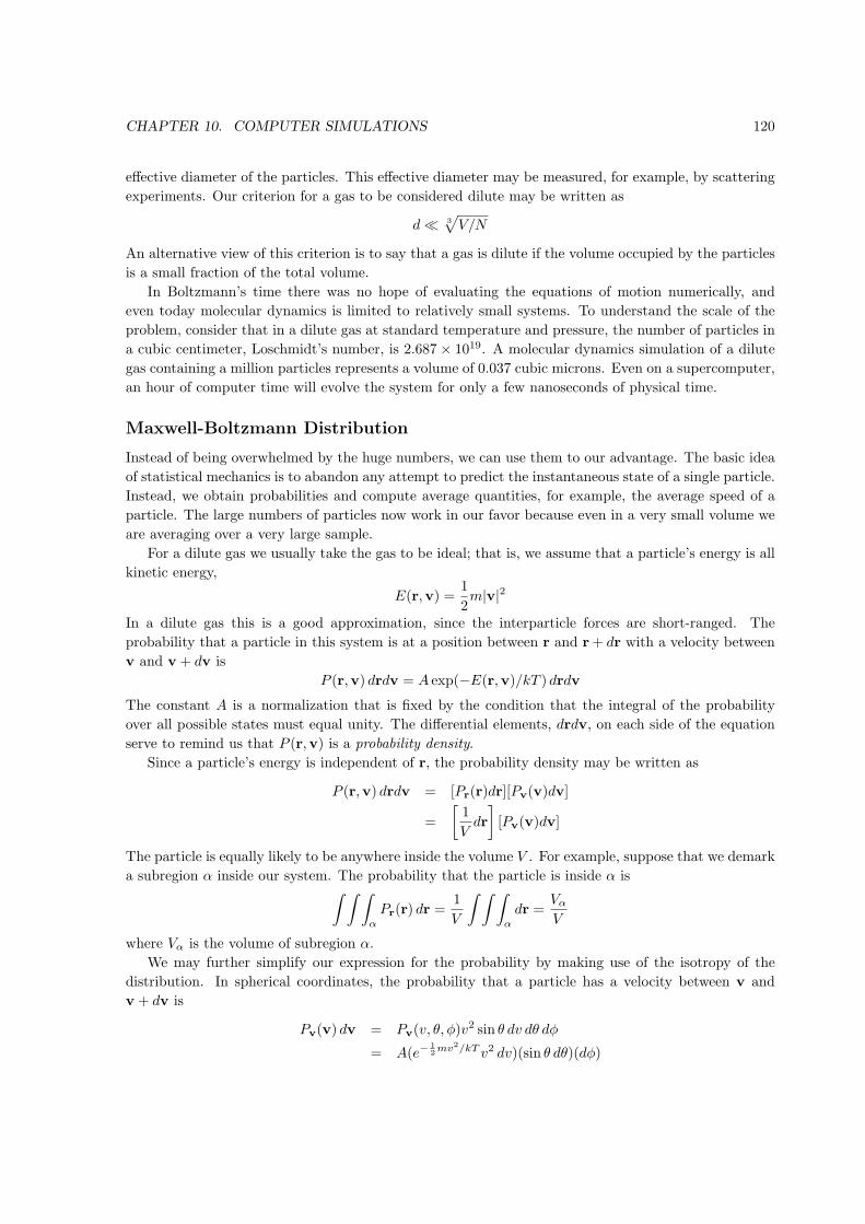
CHAPTER 10. COMPUTER SIMULATIONS 120
effective diameter of the particles. This effective diameter may be measured, for example, by scattering
experiments. Our criterion for a gas to be considered dilute may be written as
d ≪ 3√
V/N
An alternative view of this criterion is to say that a gas is dilute if the volume occupied by the particles
is a small fraction of the total volume.
In Boltzmann’s time there was no hope of evaluating the equations of motion numerically, and
even today molecular dynamics is limited to relatively small systems. To understand the scale of the
problem, consider that in a dilute gas at standard temperature and pressure, the number of particles in
a cubic centimeter, Loschmidt’s number, is 2.687× 10¹⁹. A molecular dynamics simulation of a dilute
gas containing a million particles represents a volume of 0.037 cubic microns. Even on a supercomputer,
an hour of computer time will evolve the system for only a few nanoseconds of physical time.
Maxwell-Boltzmann Distribution
Instead of being overwhelmed by the huge numbers, we can use them to our advantage. The basic idea
of statistical mechanics is to abandon any attempt to predict the instantaneous state of a single particle.
Instead, we obtain probabilities and compute average quantities, for example, the average speed of a
particle. The large numbers of particles now work in our favor because even in a very small volume we
are averaging over a very large sample.
For a dilute gas we usually take the gas to be ideal; that is, we assume that a particle’s energy is all
kinetic energy,
E(r,v) =1
2m|v|2
In a dilute gas this is a good approximation, since the interparticle forces are short-ranged. The
probability that a particle in this system is at a position between r and r+ dr with a velocity between
v and v + dv is
P (r,v) drdv = A exp(−E(r,v)/kT ) drdv
The constant A is a normalization that is fixed by the condition that the integral of the probability
over all possible states must equal unity. The differential elements, drdv, on each side of the equation
serve to remind us that P (r,v) is a probability density.
Since a particle’s energy is independent of r, the probability density may be written as
P (r,v) drdv = [Pr(r)dr][Pv(v)dv]
=
[1
Vdr
][Pv(v)dv]
The particle is equally likely to be anywhere inside the volume V . For example, suppose that we demark
a subregion α inside our system. The probability that the particle is inside α is∫ ∫ ∫α
Pr(r) dr =1
V
∫ ∫ ∫α
dr =Vα
V
where Vα is the volume of subregion α.
We may further simplify our expression for the probability by making use of the isotropy of the
distribution. In spherical coordinates, the probability that a particle has a velocity between v and
v + dv is
Pv(v) dv = Pv(v, θ, ϕ)v2 sin θ dv dθ dϕ
= A(e−12mv2/kT v2 dv)(sin θ dθ)(dϕ)
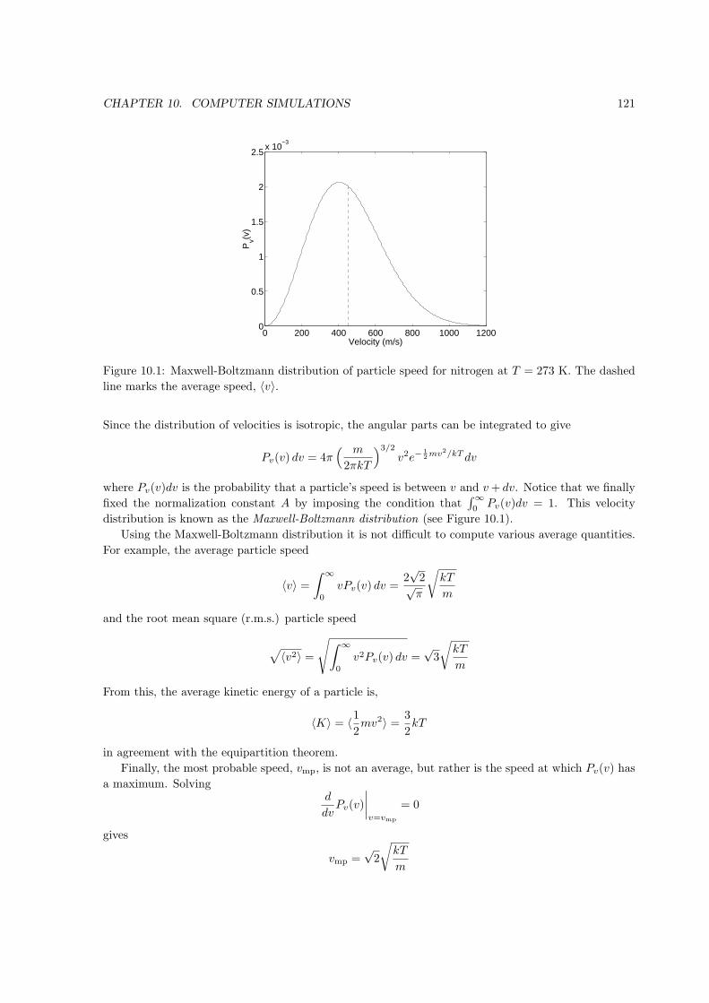
CHAPTER 10. COMPUTER SIMULATIONS 121
0 200 400 600 800 1000 12000
0.5
1
1.5
2
2.5x 10
−3
Velocity (m/s)
Pv(v
)
Figure 10.1: Maxwell-Boltzmann distribution of particle speed for nitrogen at T = 273 K. The dashed
line marks the average speed, ⟨v⟩.
Since the distribution of velocities is isotropic, the angular parts can be integrated to give
Pv(v) dv = 4π( m
2πkT
)3/2v2e−
12mv2/kT dv
where Pv(v)dv is the probability that a particle’s speed is between v and v+ dv. Notice that we finally
fixed the normalization constant A by imposing the condition that∫∞0
Pv(v)dv = 1. This velocity
distribution is known as the Maxwell-Boltzmann distribution (see Figure 10.1).
Using the Maxwell-Boltzmann distribution it is not difficult to compute various average quantities.
For example, the average particle speed
⟨v⟩ =∫ ∞
0
vPv(v) dv =2√2√π
√kT
m
and the root mean square (r.m.s.) particle speed
√⟨v2⟩ =
√∫ ∞
0
v2Pv(v) dv =√3
√kT
m
From this, the average kinetic energy of a particle is,
⟨K⟩ = ⟨12mv2⟩ = 3
2kT
in agreement with the equipartition theorem.
Finally, the most probable speed, vmp, is not an average, but rather is the speed at which Pv(v) has
a maximum. Solvingd
dvPv(v)
∣∣∣∣v=vmp
= 0
gives
vmp =√2
√kT
m
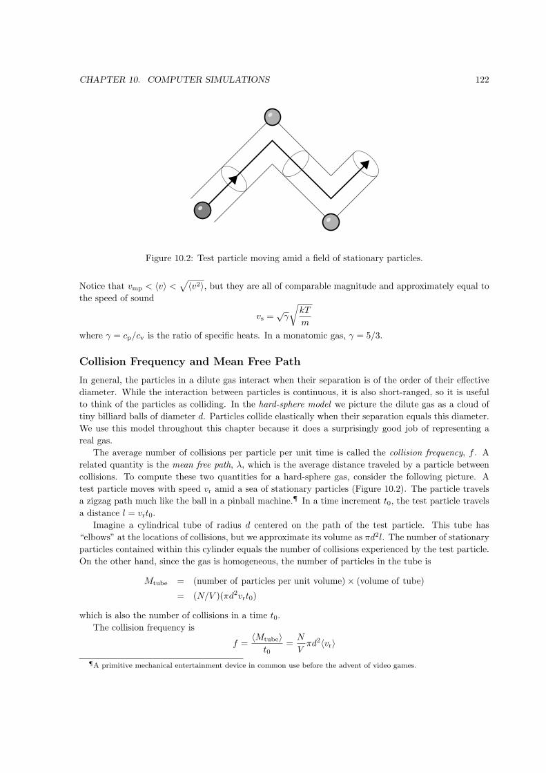
CHAPTER 10. COMPUTER SIMULATIONS 122
Figure 10.2: Test particle moving amid a field of stationary particles.
Notice that vmp < ⟨v⟩ <√⟨v2⟩, but they are all of comparable magnitude and approximately equal to
the speed of sound
vs =√γ
√kT
m
where γ = cp/cv is the ratio of specific heats. In a monatomic gas, γ = 5/3.
Collision Frequency and Mean Free Path
In general, the particles in a dilute gas interact when their separation is of the order of their effective
diameter. While the interaction between particles is continuous, it is also short-ranged, so it is useful
to think of the particles as colliding. In the hard-sphere model we picture the dilute gas as a cloud of
tiny billiard balls of diameter d. Particles collide elastically when their separation equals this diameter.
We use this model throughout this chapter because it does a surprisingly good job of representing a
real gas.
The average number of collisions per particle per unit time is called the collision frequency, f . A
related quantity is the mean free path, λ, which is the average distance traveled by a particle between
collisions. To compute these two quantities for a hard-sphere gas, consider the following picture. A
test particle moves with speed vr amid a sea of stationary particles (Figure 10.2). The particle travels
a zigzag path much like the ball in a pinball machine.¶ In a time increment t0, the test particle travels
a distance l = vrt0.
Imagine a cylindrical tube of radius d centered on the path of the test particle. This tube has
“elbows” at the locations of collisions, but we approximate its volume as πd2l. The number of stationary
particles contained within this cylinder equals the number of collisions experienced by the test particle.
On the other hand, since the gas is homogeneous, the number of particles in the tube is
Mtube = (number of particles per unit volume)× (volume of tube)
= (N/V )(πd2vrt0)
which is also the number of collisions in a time t0.
The collision frequency is
f =⟨Mtube⟩
t0=
N
Vπd2⟨vr⟩
¶A primitive mechanical entertainment device in common use before the advent of video games.
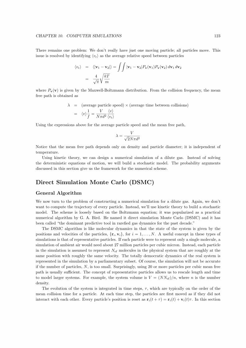
CHAPTER 10. COMPUTER SIMULATIONS 123
There remains one problem: We don’t really have just one moving particle; all particles move. This
issue is resolved by identifying ⟨vr⟩ as the average relative speed between particles
⟨vr⟩ = ⟨|v1 − v2|⟩ =∫ ∫
|v1 − v2|Pv(v1)Pv(v2) dv1 dv2
=4√π
√kT
m
where Pv(v) is given by the Maxwell-Boltzmann distribution. From the collision frequency, the mean
free path is obtained as
λ = (average particle speed)× (average time between collisions)
= ⟨v⟩ 1f=
V
Nπd2⟨v⟩⟨vr⟩
Using the expressions above for the average particle speed and the mean free path,
λ =V√
2Nπd2
Notice that the mean free path depends only on density and particle diameter; it is independent of
temperature.
Using kinetic theory, we can design a numerical simulation of a dilute gas. Instead of solving
the deterministic equations of motion, we will build a stochastic model. The probability arguments
discussed in this section give us the framework for the numerical scheme.
Direct Simulation Monte Carlo (DSMC)
General Algorithm
We now turn to the problem of constructing a numerical simulation for a dilute gas. Again, we don’t
want to compute the trajectory of every particle. Instead, we’ll use kinetic theory to build a stochastic
model. The scheme is loosely based on the Boltzmann equation; it was popularized as a practical
numerical algorithm by G. A. Bird. He named it direct simulation Monte Carlo (DSMC) and it has
been called “the dominant predictive tool in rarefied gas dynamics for the past decade.”
The DSMC algorithm is like molecular dynamics in that the state of the system is given by the
positions and velocities of the particles, ri,vi, for i = 1, . . . , N . A useful concept in these types of
simulations is that of representative particles. If each particle were to represent only a single molecule, a
simulation of ambient air would need about 27 million particles per cubic micron. Instead, each particle
in the simulation is assumed to represent Nef molecules in the physical system that are roughly at the
same position with roughly the same velocity. The totally democratic dynamics of the real system is
represented in the simulation by a parliamentary subset. Of course, the simulation will not be accurate
if the number of particles, N , is too small. Surprisingly, using 20 or more particles per cubic mean free
path is usually sufficient. The concept of representative particles allows us to rescale length and time
to model larger systems. For example, the system volume is V = (NNef)/n, where n is the number
density.
The evolution of the system is integrated in time steps, τ , which are typically on the order of the
mean collision time for a particle. At each time step, the particles are first moved as if they did not
interact with each other. Every particle’s position is reset as ri(t+ τ) = ri(t) + vi(t)τ . In this section
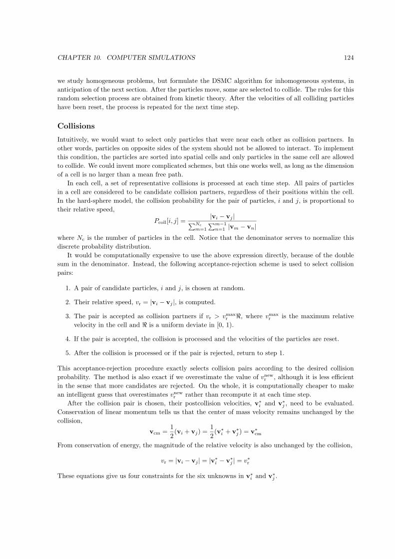
CHAPTER 10. COMPUTER SIMULATIONS 124
we study homogeneous problems, but formulate the DSMC algorithm for inhomogeneous systems, in
anticipation of the next section. After the particles move, some are selected to collide. The rules for this
random selection process are obtained from kinetic theory. After the velocities of all colliding particles
have been reset, the process is repeated for the next time step.
Collisions
Intuitively, we would want to select only particles that were near each other as collision partners. In
other words, particles on opposite sides of the system should not be allowed to interact. To implement
this condition, the particles are sorted into spatial cells and only particles in the same cell are allowed
to collide. We could invent more complicated schemes, but this one works well, as long as the dimension
of a cell is no larger than a mean free path.
In each cell, a set of representative collisions is processed at each time step. All pairs of particles
in a cell are considered to be candidate collision partners, regardless of their positions within the cell.
In the hard-sphere model, the collision probability for the pair of particles, i and j, is proportional to
their relative speed,
Pcoll[i, j] =|vi − vj |∑Nc
m=1
∑m−1n=1 |vm − vn|
where Nc is the number of particles in the cell. Notice that the denominator serves to normalize this
discrete probability distribution.
It would be computationally expensive to use the above expression directly, because of the double
sum in the denominator. Instead, the following acceptance-rejection scheme is used to select collision
pairs:
1. A pair of candidate particles, i and j, is chosen at random.
2. Their relative speed, vr = |vi − vj |, is computed.
3. The pair is accepted as collision partners if vr > vmaxr ℜ, where vmax
r is the maximum relative
velocity in the cell and ℜ is a uniform deviate in [0, 1).
4. If the pair is accepted, the collision is processed and the velocities of the particles are reset.
5. After the collision is processed or if the pair is rejected, return to step 1.
This acceptance-rejection procedure exactly selects collision pairs according to the desired collision
probability. The method is also exact if we overestimate the value of vnewr , although it is less efficient
in the sense that more candidates are rejected. On the whole, it is computationally cheaper to make
an intelligent guess that overestimates vnewr rather than recompute it at each time step.
After the collision pair is chosen, their postcollision velocities, v∗i and v∗
j , need to be evaluated.
Conservation of linear momentum tells us that the center of mass velocity remains unchanged by the
collision,
vcm =1
2(vi + vj) =
1
2(v∗
i + v∗j ) = v∗
cm
From conservation of energy, the magnitude of the relative velocity is also unchanged by the collision,
vr = |vi − vj | = |v∗i − v∗
j | = v∗r
These equations give us four constraints for the six unknowns in v∗i and v∗
j .
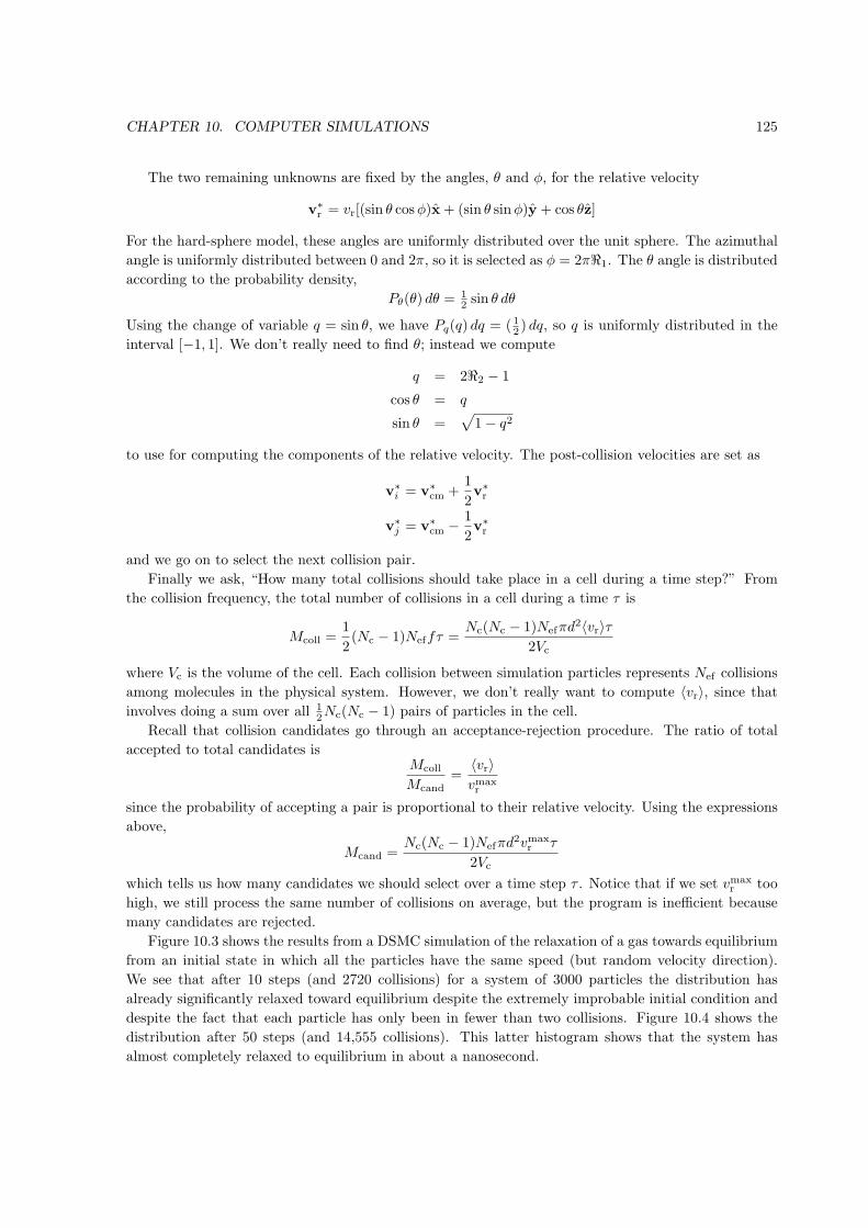
CHAPTER 10. COMPUTER SIMULATIONS 125
The two remaining unknowns are fixed by the angles, θ and ϕ, for the relative velocity
v∗r = vr[(sin θ cosϕ)x+ (sin θ sinϕ)y + cos θz]
For the hard-sphere model, these angles are uniformly distributed over the unit sphere. The azimuthal
angle is uniformly distributed between 0 and 2π, so it is selected as ϕ = 2πℜ1. The θ angle is distributed
according to the probability density,
Pθ(θ) dθ = 12 sin θ dθ
Using the change of variable q = sin θ, we have Pq(q) dq = ( 12 ) dq, so q is uniformly distributed in the
interval [−1, 1]. We don’t really need to find θ; instead we compute
q = 2ℜ2 − 1
cos θ = q
sin θ =√1− q2
to use for computing the components of the relative velocity. The post-collision velocities are set as
v∗i = v∗
cm +1
2v∗r
v∗j = v∗
cm − 1
2v∗r
and we go on to select the next collision pair.
Finally we ask, “How many total collisions should take place in a cell during a time step?” From
the collision frequency, the total number of collisions in a cell during a time τ is
Mcoll =1
2(Nc − 1)Neffτ =
Nc(Nc − 1)Nefπd2⟨vr⟩τ
2Vc
where Vc is the volume of the cell. Each collision between simulation particles represents Nef collisions
among molecules in the physical system. However, we don’t really want to compute ⟨vr⟩, since that
involves doing a sum over all 12Nc(Nc − 1) pairs of particles in the cell.
Recall that collision candidates go through an acceptance-rejection procedure. The ratio of total
accepted to total candidates isMcoll
Mcand=
⟨vr⟩vmaxr
since the probability of accepting a pair is proportional to their relative velocity. Using the expressions
above,
Mcand =Nc(Nc − 1)Nefπd
2vmaxr τ
2Vc
which tells us how many candidates we should select over a time step τ . Notice that if we set vmaxr too
high, we still process the same number of collisions on average, but the program is inefficient because
many candidates are rejected.
Figure 10.3 shows the results from a DSMC simulation of the relaxation of a gas towards equilibrium
from an initial state in which all the particles have the same speed (but random velocity direction).
We see that after 10 steps (and 2720 collisions) for a system of 3000 particles the distribution has
already significantly relaxed toward equilibrium despite the extremely improbable initial condition and
despite the fact that each particle has only been in fewer than two collisions. Figure 10.4 shows the
distribution after 50 steps (and 14,555 collisions). This latter histogram shows that the system has
almost completely relaxed to equilibrium in about a nanosecond.

CHAPTER 10. COMPUTER SIMULATIONS 126
50 150 250 350 450 550 650 750 850 95010500
500
1000
1500Final distrib., Time = 3.22864e−010 sec.
Speed (m/s)
Num
ber
Figure 10.3: Speed distribution as obtained from dsmceq for N = 3000 particles. After 10 time steps,
there have been 2720 collisions.
We can also use this simulation to compute
H(t) =∑bins
∆vNh(v)
Nln
Nh(v)
N
where Nh(v) is the number of particles in a histogram bin of width ∆v. This H-function was introduced
by Boltzmann and it is proportional to the negative of the entropy in the system. Since the system is
initially out of equilibrium, H decreases with time until the system equilibrates, as shown in Figure 10.5.
For a full description of the DSMC methods, including programming examples, see my textbook
Numerical Methods for Physics. Makes for great summer reading at the beach!
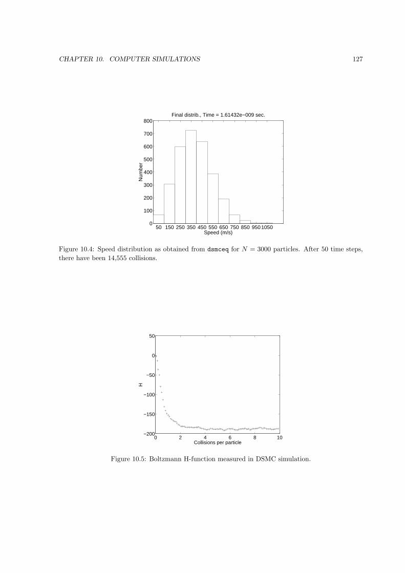
CHAPTER 10. COMPUTER SIMULATIONS 127
50 150 250 350 450 550 650 750 850 95010500
100
200
300
400
500
600
700
800Final distrib., Time = 1.61432e−009 sec.
Speed (m/s)
Num
ber
Figure 10.4: Speed distribution as obtained from dsmceq for N = 3000 particles. After 50 time steps,
there have been 14,555 collisions.
0 2 4 6 8 10−200
−150
−100
−50
0
50
Collisions per particle
H
Figure 10.5: Boltzmann H-function measured in DSMC simulation.


![Bio Soil Interactions Engineering Workshop1].pdf · Bio‐Soil Interactions & Engineering Workshop ... Notes. Notes. Notes. Notes. Notes. Notes. ... Electrokinetic and Electrolytic](https://img.pdfslide.net/doc/110x75/5e7be480f39bf41290742405/bio-soil-interactions-engineering-workshop-1pdf-bioasoil-interactions-.jpg)