Lecture34

NPTEL- Probability and Distributions

Dept. of Mathematics and Statistics Indian Institute of Technology, Kanpur 1

MODULE 6

RANDOM VECTOR AND ITS JOINT DISTRIBUTION

LECTURE 34

Topics

6.10.2 Transformation of Variables Technique

6.10.2.1 Distribution of Order Statistics

6.10.2.2 Distribution of Normalized Spacing’s of Exponential Distribution

For finding the probability distributions of functions of a random vector of absolutely

continuous type we have the following theorem.

Theorem 10.2.2

Let 𝑋 = 𝑋1, … , 𝑋𝑝 be a random vector of absolutely continuous type with a joint p.d.f.

𝑓𝑋 ∙ and support 𝑆𝑋 = 𝑥 ∈ ℝ𝑝 : 𝑓𝑋 𝑥 > 0 . Let 𝑆1, … , 𝑆𝑘 be open subset of ℝ𝑝 such

that 𝑆𝑖 ∩ 𝑆𝑗 = 𝜙, if 𝑖 ≠ 𝑗, and 𝑆𝑖 = 𝑆𝑋𝑘𝑖=1 . Suppose that ℎ𝑗 : ℝ𝑝 → ℝ , 𝑗 = 1, … , 𝑝, are 𝑝

Borel functions such that on each 𝑆𝑖 , ℎ = ℎ1 , … , ℎ𝑝 : 𝑆𝑖 → ℝ𝑝 is one-to-one with inverse

transformation ℎ𝑖−1 𝑡 = ℎ1,𝑖

−1 𝑡 , … , ℎ𝑝 ,𝑖−1 𝑡 say , 𝑖 = 1, … , 𝑘 . Further suppose that

ℎ𝑗 ,𝑖−1 𝑡 , 𝑗 = 1, … , 𝑝, 𝑖 = 1, … , 𝑘, have continuous partial derivatives and the Jacobian

determinants

𝐽𝑖 =

𝜕ℎ1,𝑖−1 𝑡

𝜕𝑡1⋯

𝜕ℎ1,𝑖−1 𝑡

𝜕𝑡𝑝

𝜕ℎ2,𝑖−1 𝑡

𝜕𝑡1⋯

𝜕ℎ2,𝑖−1 𝑡

𝜕𝑡𝑝⋮

𝜕ℎ𝑝 ,𝑖−1 𝑡

𝜕𝑡1

⋮⋯

⋮𝜕ℎ𝑝 ,𝑖

−1 𝑡

𝜕𝑡𝑝

≠ 0, 𝑖 = 1, … , 𝑝.

Define ℎ 𝑆𝑗 = ℎ 𝑥 = ℎ1 𝑥 , … , ℎ𝑝 𝑥 ∈ ℝ𝑝 : 𝑥 ∈ 𝑆𝑗 , 𝑗 = 1, … , 𝑝 and 𝑇𝑗 =

ℎ𝑗 𝑋1, … , 𝑋𝑝 , 𝑗 = 1, … , 𝑝 . Then the random vector 𝑇 = 𝑇1, … , 𝑇𝑝 is of absolutely

continuous type with joint p.d.f.



𝑓𝑇 𝑡 = 𝑓𝑋 ℎ1,𝑗−1 𝑡 , … , ℎ𝑝 ,𝑗

−1 𝑡 𝐽𝑗

𝑘

𝑗 =1

𝐼ℎ 𝑠𝑗 𝑡 . ▄

We shall not provide the proof of the above theorem. The idea of the proof of the above

theorem is similar to that of Theorem 2.2, Module 3. In the proof of the theorem, the joint

distribution function of 𝑇 is written in the form of multiple integrals which are simplified

by making change of variables using change of variable Theorem of multivariable

calculus.

The following corollary is immediate from Theorem 10.2.2.

Corollary 10.2.1

Let 𝑋 = 𝑋1, … , 𝑋𝑝 be a random vector of absolutely continuous type with a joint p.d.f.

𝑓𝑋 ∙ and support 𝑆𝑋 = 𝑥 ∈ ℝ𝑝 : 𝑓𝑋 𝑥 > 0 , an open set in ℝ𝑝 . Suppose that ℎ𝑗 : ℝ𝑝 →

ℝ, 𝑗 = 1, … , 𝑝, are 𝑝 Borel functions such that ℎ = ℎ1, … , ℎ𝑝 : 𝑆𝑋 → ℝ𝑝 is one-to-one

with inverse transformation ℎ−1 𝑡 = (ℎ1−1 𝑡 , … , ℎ𝑝

−1 𝑡 ) (say). Further suppose that

ℎ𝑖−1, 𝑖 = 1, … , 𝑝, have continuous partial derivatives and the Jacobian determinant

𝐽 =

𝜕ℎ1−1 𝑡

𝜕𝑡1⋯

𝜕ℎ1−1 𝑡

𝜕𝑡𝑝

𝜕ℎ2−1 𝑡

𝜕𝑡1⋯

𝜕ℎ2−1 𝑡

𝜕𝑡𝑝⋮

𝜕ℎ𝑝−1 𝑡

𝜕𝑡1

⋯𝜕ℎ𝑝

−1 𝑡

𝜕𝑡𝑝

≠ 0.

Define ℎ 𝑆𝑋 = ℎ 𝑥 = ℎ1 𝑥 , ⋯ , ℎ𝑝 𝑥 ) ∈ ℝ𝑝 : 𝑥 ∈ 𝑆𝑋 and 𝑇𝑗 = ℎ𝑗 𝑋1, … , 𝑋𝑝 , 𝑗 =

1, … , 𝑝. Then the random vector 𝑇 = 𝑇1, … , 𝑇𝑝 is of absolutely continuous type with

joint p.d.f.

𝑓𝑇 𝑡 = 𝑓𝑋 ℎ1−1 𝑡 , ⋯ , ℎ𝑝

−1 𝑡 𝐽 𝐼ℎ 𝑆𝑋 𝑡 . ▄

Remark 10.2.1

Let 𝑋 = 𝑋1, … , 𝑋𝑝 be a random vector of absolutely continuous type with joint p.d.f. 𝑓𝑋

and let 𝑆𝑋 = 𝑥 ∈ ℝ𝑝 : 𝑓𝑋 𝑥 > 0 .Suppose that we are interested in finding the joint

probability distribution of random vector 𝑇 = 𝑇1, … , 𝑇𝑘 = ℎ1 𝑋 , … , ℎ𝑘 𝑋 ), where



𝑘 ∈ 1, … , 𝑝 and ℎ𝑖 : ℝ𝑝 → ℝ, 𝑖 = 1, … , 𝑘, are some Borel functions. For this we shall

define 𝑝 − 𝑘 additional auxiliary Borel functions ℎ𝑖 : ℝ𝑝 → ℝ, 𝑖 = 𝑘 + 1, … , 𝑝, such that

the transformation ℎ = ℎ1 , … , ℎ𝑝 : 𝑆𝑋 → ℝ𝑝 , satisfies the assumptions of Theorem

10.2.2/Corollary 10.2.1. Then an application of Theorem 10.2.2/Corollary 10.2.1 will

provide the joint p.d.f. 𝑓𝑇 𝑡1, … , 𝑡𝑝 of 𝑇 = 𝑇1, … , 𝑇𝑝 from which marginal joint p.d.f.

of 𝑈 = 𝑇1, … , 𝑇𝑘 is obtained by integrating out unwanted variables 𝑡𝑘+1, … , 𝑡𝑝 in

𝑓𝑇 𝑢1, … , 𝑢𝑘 , 𝑡𝑘+1, … , 𝑡𝑝 .

Example 10.2.8

Let 𝑋1 and 𝑋2 be independent and identically distributed random variables with common

p.d.f.

𝑓 𝑥 =

1

2, if − 2 < 𝑥 < −1

1

6, if 0 < 𝑥 < 3

0, otherwise

.

Find the p.d.f. of 𝑌1 = 𝑋1 + 𝑋2 .

Solution. The joint p.d.f. of 𝑋 = 𝑋1, 𝑋2 is given by

𝑓𝑋 𝑥1, 𝑥2 = 𝑓 𝑥1 𝑓 𝑥2

=

1

4, if 𝑥1, 𝑥2 ∈ −2, −1 × −2, −1

1

12, if 𝑥1, 𝑥2 ∈ −2, −1 × 0, 3 ∪ 0, 3 × −2, −1 .

1

36, if 𝑥1, 𝑥2 ∈ 0, 3 × 0, 3

0, otherwise

Define the auxiliary random variable 𝑌2 = 𝑋1 . We have

𝑆𝑋 = 𝑥 = 𝑥1, 𝑥2 ∈ ℝ2: 𝑓𝑋 𝑥1, 𝑥2 > 0

= 𝑆1 ∪ 𝑆2 ∪ 𝑆3 ∪ 𝑆4,

where 𝑆1 = −2, −1 2, 𝑆2 = −2, −1 × 0, 3 , 𝑆3 = 0, 3 × −2, −1 and 𝑆4 =

0, 3 2. Let ℎ = ℎ1, ℎ2 : ℝ2 → ℝ2 be defined by

ℎ1 𝑥1, 𝑥2 = 𝑥1 + 𝑥2 and ℎ2 𝑥1, 𝑥2 = 𝑥1 , 𝑥 = 𝑥1, 𝑥2 ∈ ℝ2 .



Then 𝑌1 = ℎ1 𝑋1, 𝑋2 , 𝑌2 = ℎ2 𝑋1, 𝑋2 , 𝑆𝑖 ∩ 𝑆𝑗 = 𝜙, 𝑖 ≠ 𝑗 and on each 𝑆𝑖 , 𝑖 = 1, 2, 3, 4,

ℎ = ℎ1, ℎ2 : 𝑆𝑖 → ℝ2 is one-to-one. Under the notation of Theorem 10.2.2 we have

ℎ1,1−1 𝑡 = −𝑡2, ℎ2,1

−1 𝑡 = 𝑡2 − 𝑡1, 𝐽1 = 0 −1

−1 1 = −1;

ℎ1,2−1 𝑡 = −𝑡2, ℎ2,2

−1 𝑡 = 𝑡1 − 𝑡2 , 𝐽2 = 0 −11 −1

= 1;

ℎ1,3−1 𝑡 = 𝑡2, ℎ2,3

−1 𝑡 = 𝑡2 − 𝑡1 , 𝐽3 = 0 1

−1 1 = 1;

ℎ1,4−1 𝑡 = 𝑡2, ℎ2,4

−1 𝑡 = 𝑡1 − 𝑡2 , 𝐽4 = 0 11 −1

= −1;

ℎ 𝑆1 = 𝑡1, 𝑡2 ∈ ℝ2: −2 < −𝑡2 < −1 , −2 < 𝑡2 − 𝑡1 < −1

= 𝑡1, 𝑡2 ∈ ℝ2: 𝑡2 + 1 < 𝑡1 < 𝑡2 + 2, 1 < 𝑡2 < 2 ;

ℎ 𝑆2 = 𝑡1, 𝑡2 ∈ ℝ2: −2 < −𝑡2 < −1, 0 < 𝑡1 − 𝑡2 < 3

= 𝑡1, 𝑡2 ∈ ℝ2: 𝑡2 < 𝑡1 < 𝑡2 + 3, 1 < 𝑡2 < 2 ;

ℎ 𝑆3 = 𝑡1, 𝑡2 ∈ ℝ2: 0 < 𝑡2 < 3 , −2 < 𝑡2 − 𝑡1 < −1

= 𝑡1, 𝑡2 ∈ ℝ2: 𝑡2 + 1 < 𝑡1 < 𝑡2 + 2, 0 < 𝑡2 < 3

and

ℎ 𝑆4 = 𝑡1, 𝑡2 ∈ ℝ2: 0 < 𝑡2 < 3 ,0 < 𝑡1 − 𝑡2 < 3

= 𝑡1, 𝑡2 ∈ ℝ2: 𝑡2 < 𝑡1 < 𝑡2 + 3, 0 < 𝑡2 < 3 .

Consequently the joint p.d.f. of 𝑌 = 𝑌1, 𝑌2 is given by

𝑓𝑌 𝑡1, 𝑡2 = 𝑓𝑋 ℎ1,𝑗−1 𝑡 , ℎ2,𝑗

−1 𝑡 𝐽𝑗 𝐼ℎ 𝑆𝑗 (𝑡)

4

𝑗 =1

= 𝑓𝑋 −𝑡2, 𝑡2−𝑡1 𝐼ℎ 𝑆1 𝑡 + 𝑓𝑋 −𝑡2, 𝑡1−𝑡2 𝐼ℎ 𝑆2 𝑡

+𝑓𝑋 𝑡2, 𝑡2−𝑡1 𝐼ℎ 𝑆3 (𝑡) + 𝑓𝑋 𝑡2, 𝑡1−𝑡2 𝐼ℎ 𝑆4 (𝑡)



=

1

36, if 𝑡2 < 𝑡1 < 𝑡2 + 1, 0 < 𝑡2 < 1

1

12+

1

36, if 𝑡2 + 1 < 𝑡1 < 𝑡2 + 2, 0 < 𝑡2 < 1

1

36, if 𝑡2 + 2 < 𝑡1 < 𝑡2 + 3, 0 < 𝑡2 < 1

1

12+

1

36, if 𝑡2 < 𝑡1 < 𝑡2 + 1, 1 < 𝑡2 < 2

1

4+

1

12+

1

12+

1

36, if 𝑡2 + 1 < 𝑡1 < 𝑡2 + 2, 1 < 𝑡2 < 2

1

12+

1

36, if 𝑡2 + 2 < 𝑡1 < 𝑡2 + 3, 1 < 𝑡2 < 2

1

36, if 𝑡2 < 𝑡1 < 𝑡2 + 1, 2 < 𝑡2 < 3

1

12+

1

36, if 𝑡2 + 1 < 𝑡1 < 𝑡2 + 2, 2 < 𝑡2 < 3

1

36, if 𝑡2 + 2 < 𝑡1 < 𝑡2 + 3, 2 < 𝑡2 < 3

0, otherwise

=

1

36, if 0 < 𝑡1 < 2, max 0, 𝑡1 − 1 < 𝑡2 < min 1, 𝑡1

or 2 < 𝑡1 < 4, max 0, 𝑡1 − 3 < 𝑡2 < min 1, 𝑡1 − 2

or 2 < 𝑡1 < 4, max 2, 𝑡1 − 1 < 𝑡2 < min 3, 𝑡1

or 4 < 𝑡1 < 6, max 2, 𝑡1 − 3 < 𝑡2 < min 3, 𝑡1 − 2

1

9, if 1 < 𝑡1 < 3, max 0, 𝑡1 − 2 < 𝑡2 < min 1, 𝑡1 − 1

or 1 < 𝑡1 < 3, max 1, 𝑡1 − 1 < 𝑡2 < min 2, 𝑡1

or 3 < 𝑡1 < 5, max 1, 𝑡1 − 3 < 𝑡2 < min 2, 𝑡1 − 2

or 3 < 𝑡1 < 5, max 2, 𝑡1 − 2 < 𝑡2 < min 3, 𝑡1 − 1 4

9, if 2 < 𝑡1 < 4, max 1, 𝑡1 − 2 < 𝑡2 < min 2, 𝑡1 − 1

0, otherwise

.

Then the marginal p.d.f. of 𝑌1 is given by



𝑓𝑌1 𝑡1 = 𝑓𝑌

∞

−∞

𝑡1, 𝑡2 𝑑𝑡2, 𝑡1 ∈ ℝ.

For 𝑡1 ∈ 0, 1

𝑓𝑌1 𝑡1 =

min 1, 𝑡1 − max 0, 𝑡1 − 1

36

=𝑡1

36;

for 𝑡1 ∈ 1, 2

𝑓𝑌1 𝑡1 =

min 1, 𝑡1 − max 0, 𝑡1 − 1

36+

min 1, 𝑡1 − 1 − max 0, 𝑡1 − 2

9

+min 2, 𝑡1 − max 1, 𝑡1 − 1

9

=7𝑡1 − 6

36;

for 𝑡1 ∈ 2, 3

𝑓𝑌1 𝑡1 =

min 1, 𝑡1 − 2 − max 0, 𝑡1 − 3

36+

min 3, 𝑡1 − max 2, 𝑡1 − 1

36

+min 1, 𝑡1 − 1 − max 0, 𝑡1 − 2

9+

min 2, 𝑡1 − max 1, 𝑡1 − 1

9

+4 min 2, 𝑡1 − 1 − max 1, 𝑡1 − 2

9

=5𝑡1 − 6

18;

for 𝑡1 ∈ 3, 4

𝑓𝑌1 𝑡1 =

min 1, 𝑡1 − 2 − max 0, 𝑡1 − 3

36+

min 3, 𝑡1 − max 2, 𝑡1 − 1

36

+min 2, 𝑡1 − 2 − max 1, 𝑡1 − 3

9+

min 3, 𝑡1 − 1 − max 2, 𝑡1 − 2

9

+4 min 2, 𝑡1 − 1 − max 1, 𝑡1 − 2

9



=24 − 5𝑡1

18;

for 𝑡1 ∈ 4, 5

𝑓𝑌1 𝑡1 =

min 3, 𝑡1 − 2 − max 2, 𝑡1 − 3

36+

min 2, 𝑡1 − 2 − max 1, 𝑡1 − 3

9

+min 3, 𝑡1 − 1 − max 2, 𝑡1 − 2

9

=36 − 7𝑡1

36;

and, for 𝑡1 ∈ 5, 6

𝑓𝑌1 𝑡1 =

min 3, 𝑡1 − 2 − max 2, 𝑡1 − 3

36

=6 − 𝑡1

36.

Therefore the p.d.f. of 𝑌1 = 𝑋1 + 𝑋2 is given by

𝑓𝑌1(𝑡1) =

𝑡1

36, if 0 < 𝑡1 < 1

7𝑡1 − 6

36, if 1 < 𝑡1 < 2

5𝑡1 − 6

18, if 2 < 𝑡1 < 3

24 − 5𝑡1

18, if 3 < 𝑡1 < 4

36 − 7𝑡1

36, if 4 < 𝑡1 < 5

6 − 𝑡1

36, if 5 < 𝑡1 < 6

0, otherwise

. ▄

6.10.2.1 Distribution of Order Statistics

Example 10.2.9

Let 𝑋1, … , 𝑋𝑛 be a random sample of absolutely continuous type random variables having

a common p.d.f. 𝑓 ∙ , the common distribution function 𝐹(⋅) and a common support

𝑆 = 𝑥 ∈ ℝ: 𝑓 𝑥 > 0 , an open set in ℝ. Let 𝑋1:𝑛 , … , 𝑋𝑛:𝑛 denote the order statistics of



𝑋1, … , 𝑋𝑛 , i.e.,𝑋𝑟:𝑛 = r-th smallest of 𝑋1, … , 𝑋𝑛 , 𝑟 = 1, … , 𝑛. For notational convenience,

let 𝑌𝑟 = 𝑋𝑟:𝑛 , 𝑟 = 1, … , 𝑛.

(i) Find an expression for the joint distribution function of 𝑌 = 𝑌1, … , 𝑌𝑛 . Hence find

the joint p.d.f. of 𝑌;

(ii) Find the joint p.d.f. of 𝑌 directly using Theorem 10.2.2;

(iii) Using (ii), find the marginal p.d.f. of 𝑌𝑟 , 𝑟 = 1, … , 𝑛;

(iv) Using (ii), find the marginal joint p.d.f. of 𝑌𝑟 , 𝑌𝑠 , where 1 ≤ 𝑟 < 𝑠 ≤ 𝑛.

Proof. The joint p.d.f. of 𝑋 = 𝑋1, … , 𝑋𝑛 is given by

𝑓𝑋 𝑥1, … , 𝑥𝑛 = 𝑓𝑋𝑖(𝑥𝑖)

𝑛

𝑖=1

= 𝑓 𝑥𝑖

𝑛

𝑖=1

, 𝑥 = 𝑥1, … , 𝑥𝑛 ∈ ℝ𝑛 .

Let 𝑆𝑛 = Π1

, ⋯ ,Π𝑛 !

denote the set of all permutations of 1, … , 𝑛 ; here for 𝑖 ∈

1, … , 𝑛! ,Π𝑖

= Π𝑖 , 1 , … ,Π𝑖 , 𝑛 is a permutation of 1, … , 𝑛 .

(i) Since 𝑋1, … , 𝑋𝑛 is a random sample we have

𝑋1, … , 𝑋𝑛 =𝑑

𝑋Π𝑖 , 1 , … , 𝑋Π𝑖 , 𝑛

, 𝑖 ∈ 1, … , 𝑛! . (10.2.1)

Also since 𝑋 = 𝑋1, … , 𝑋𝑛 is of absolutely continuous type (as 𝑋1, … , 𝑋𝑛 are of

absolutely continuous type) we have 𝑃 𝑋𝑖 = 𝑋𝑗 , for some 𝑖 ≠ 𝑗 = 0. Therefore

𝑃

𝑛 !

𝑖=1

𝑋Π𝑖 , 1 < ⋯ < 𝑋Π𝑖 , 𝑛

= 1.

Then, for 𝑦 = 𝑦1, … , 𝑦𝑛 ∈ ℝ𝑛 ,

𝐹𝑌 𝑦 = 𝑃 𝑋1:𝑛 ≤ 𝑦1, … , 𝑋𝑛 :𝑛 ≤ 𝑦𝑛

= 𝑃

𝑛 !

𝑖=1

𝑋1:𝑛 ≤ 𝑦1, … , 𝑋𝑛 :𝑛 ≤ 𝑦𝑛 , 𝑋Π𝑖 , 1 < ⋯ < 𝑋Π𝑖 , 𝑛

= 𝑃

𝑛 !

𝑖=1

𝑋Π𝑖 , 1 ≤ 𝑦1, … , 𝑋Π𝑖 , 𝑛

≤ 𝑦𝑛 , 𝑋Π𝑖 , 1 < ⋯ < 𝑋Π𝑖 , 𝑛

= 𝑃

𝑛 !

𝑖=1

𝑋1 ≤ 𝑦1, … , 𝑋𝑛 ≤ 𝑦𝑛 , 𝑋1 < ⋯ < 𝑋𝑛 (using (10.2.1))



= 𝑛! 𝑃 𝑋1 ≤ 𝑦1, … , 𝑋𝑛 ≤ 𝑦𝑛 , 𝑋1 < ⋯ < 𝑋𝑛

= ⋯

𝑦1

−∞

𝑛!

𝑦𝑛

−∞

𝑓 𝑥𝑖

𝑛

𝑖=1

𝐼𝐴 𝑥 𝑑𝑥𝑛 ⋯𝑑𝑥1,

where 𝐴 = 𝑥 ∈ ℝ𝑛 : −∞ < 𝑥1 < ⋯ < 𝑥𝑛 < ∞ .

It follows that 𝑌 is of absolutely continuous type with p.d.f.

𝑓𝑌 𝑦 = 𝑛! 𝑓 𝑦𝑖

𝑛

𝑖=1

𝐼𝐴 𝑦

= 𝑛! 𝑓 𝑦𝑖

𝑛

𝑖=1

, if − ∞ < 𝑦1 < ⋯ < 𝑦𝑛 < ∞

0, otherwise

.

(ii) Since 𝑋 is of absolutely continuous type we may, without loss of generality,

take 𝑆𝑋 ⊆ 𝑥 ∈ ℝ𝑛 : 𝑥𝑖 ≠ 𝑥𝑗 , ∀𝑖 ≠ 𝑗, 𝑖, 𝑗 ∈ 1, … , 𝑛 . Then 𝑆𝑋 = 𝑆𝑖𝑛 !𝑖=1 ,

where 𝑆𝑖 = 𝑥 ∈ 𝑆𝑋 : 𝑥Π𝑖 , 1 < ⋯ < 𝑥Π𝑖 , 𝑛

, 𝑖 = 1, … , 𝑛! . Define ℎ𝑖 : ℝ𝑛 → ℝ

by ℎ𝑖 𝑥 = 𝑖-th smallest of 𝑥1, … , 𝑥𝑛 , 𝑖 = 1, … , 𝑛 and ℎ = ℎ1, … , ℎ𝑛 . Then

ℎ: 𝑆𝑋 → ℝ𝑛 is not one-to-one (for each 𝑦 ∈ ℎ 𝑆𝑋 = ℎ 𝑡 : 𝑡 ∈ 𝑆𝑋 , there are

𝑛! pre-images). However, on each 𝑆𝑖 , 𝑖 = 1, … , 𝑛!, ℎ: 𝑆𝑖 → ℝ𝑛 is one-to-one

with inverse transformation ℎ𝑖−1 𝑦 = ℎ1,𝑖

−1 𝑦 , … , ℎ𝑛 ,𝑖−1 𝑦 =

𝑦Π𝑖 , 1 −1 , … , 𝑦Π𝑖 , 𝑛

−1 , where Π𝑖

−1 = Π𝑖 , 1 −1 , … ,Π𝑖 , 𝑛

−1 , 𝑖 = 1, … , 𝑛! is the inverse

permutation of Π𝑖. Under the notation of Theorem 10.2.2 each row and each

column of the Jacobian determinant 𝐽𝑖 contains one, and only one, non-zero

element which is 1. Therefore 𝐽𝑖 = ± 1, 𝑖 = 1, … , 𝑛! . Also ℎ 𝑆𝑖 =

𝑦 ∈ 𝑆𝑋 : − ∞ < 𝑦1 < ⋯ < 𝑦𝑛 < ∞ = 𝐵, say, 𝑖 = 1, … , 𝑛. Therefore the joint

p.d.f. of 𝑌 is given by

𝑓𝑌 𝑦 = 𝑓𝑋

𝑛 !

𝑖=1

𝑦Π𝑖 , 1 −1 , … , 𝑦Π𝑖 , 𝑛

−1 𝐽𝑖 𝐼ℎ 𝑆𝑖 𝑦

= 𝑓

𝑛

𝑙=1

𝑦Π𝑖 , 𝑙 −1

𝑛 !

𝑖=1

𝐼𝐵 𝑦 .



Since Π𝑖 , 1 −1 , … ,Π𝑖 , 𝑛

−1 = 1, … , 𝑛 , we have

𝑓 𝑦Π𝑖 , 𝑙 −1

𝑛

𝑙=1

= 𝑓 𝑦𝑙

𝑛

𝑙=1

, ∀𝑦 ∈ 𝐵.

Consequently

𝑓𝑌 𝑦 = 𝑓 𝑦𝑙

𝑛

𝑙=1

𝑛 !

𝑖=1

𝐼𝐵 𝑦

= 𝑛! 𝑓 𝑦𝑙

𝑛

𝑙=1

𝐼𝐵 𝑦

= 𝑛! 𝑓 𝑦𝑙

𝑛

𝑙=1

, if − ∞ < 𝑦1 < ⋯ < 𝑦𝑛 < ∞

0, otherwise

, 𝑦 ∈ 𝑆𝑋 .

(iii) The marginal p.d.f of 𝑌𝑟 𝑟 = 1, … , 𝑛 is given by

𝑓𝑌𝑟 𝑦 = ⋯

∞

−∞

⋯

∞

−∞

∞

−∞

𝑓𝑌

∞

−∞

𝑦1, … , 𝑦𝑟−1𝑦, 𝑦𝑟+1, … , 𝑦𝑛 𝑑𝑦𝑙

𝑛

𝑙=1𝑙≠𝑟

= ⋯

𝑦𝑛

𝑦

∞

𝑦

⋯

𝑦𝑟−1

−∞

𝑦

−∞

𝑦𝑟+2

𝑦

𝑛!

𝑦2

−∞

𝑓 𝑦𝑙

𝑛

𝑙=1𝑙≠𝑟

𝑓 𝑦 𝑑𝑦𝑙

𝑛

𝑙=1𝑙≠𝑟

=𝑛!

(𝑟 − 1)! (𝑛 − 𝑟)! 𝐹 𝑦 𝑟−1 1 − 𝐹 𝑦 𝑛−𝑟𝑓 𝑦 , − ∞ < 𝑦 < ∞,

since ∫ 𝑓 𝑡 𝑎

−∞𝑑𝑡 = 𝐹 𝑎 and ∫ 𝑓 𝑡

∞

𝑏𝑑𝑡 = 1 − 𝐹 𝑏 , 𝑎, 𝑏 ∈ ℝ.

(iv) As in (iii) we have

𝑓𝑌𝑟 ,𝑌𝑠 𝑥, 𝑦 = ⋯

∞

−∞

𝑛!

∞

−∞

𝑓𝑌 𝑦1, … , 𝑦𝑟−1, 𝑥, 𝑦𝑟+1, …𝑦𝑠−1, 𝑦, 𝑦𝑠+1, …𝑦𝑛 𝑑𝑦𝑙

𝑛

𝑙=1𝑙≠𝑟 ,𝑠

= ⋯

𝑦𝑛

𝑦

∞

𝑦

⋯

𝑦𝑠−1

𝑥

𝑦

𝑥

𝑦𝑠+2

𝑦

⋯

𝑦𝑟−1

−∞

𝑥

−∞

𝑦𝑟+2

𝑥

𝑛!

𝑦2

−∞

𝑓 𝑦𝑙

𝑛


𝑓 𝑥 𝑓 𝑦 𝑑𝑦𝑙

𝑛


, if 𝑥 < 𝑦



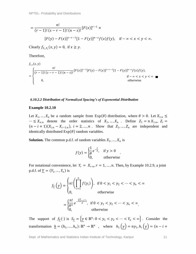
=𝑛!

𝑟 − 1 ! 𝑠 − 𝑟 − 1 ! 𝑛 − 𝑠 ! 𝐹 𝑥 𝑟−1 ×

𝐹 𝑦 − 𝐹 𝑥 𝑠−𝑟−1 1 − 𝐹 𝑦 𝑛−𝑠𝑓 𝑥 𝑓 𝑦 , if − ∞ < 𝑥 < 𝑦 < ∞.

Clearly 𝑓𝑌𝑟 ,𝑌𝑠 𝑥, 𝑦 = 0, if 𝑥 ≥ 𝑦.

Therefore,

𝑓𝑟 ,𝑠 𝑥, 𝑦

=

𝑛!

𝑟 − 1 ! 𝑠 − 𝑟 − 1 ! 𝑛 − 𝑠 ! 𝐹 𝑥 𝑟−1 𝐹 𝑦 − 𝐹 𝑥 𝑠−𝑟−1 1 − 𝐹 𝑦 𝑛−𝑠𝑓 𝑥 𝑓 𝑦 ,

if − ∞ < 𝑥 < 𝑦 < ∞

0, otherwise

.▄

6.10.2.2 Distribution of Normalized Spacing’s of Exponential Distribution

Example 10.2.10

Let 𝑋1, … , 𝑋𝑛 be a random sample from Exp 𝜃 distribution, where 𝜃 > 0. Let 𝑋1:𝑛 ≤

⋯ ≤ 𝑋𝑛:𝑛 denote the order statistics of 𝑋1, … , 𝑋𝑛 . Define 𝑍1 = 𝑛 𝑋1:𝑛 , 𝑍𝑖 =

𝑛 − 𝑖 + 1 𝑋𝑖:𝑛 − 𝑋𝑖−1:𝑛 , 𝑖 = 2, … , 𝑛 . Show that 𝑍1, … , 𝑍𝑛 are independent and

identically distributed Exp 𝜃 random variables.

Solution. The common p.d.f. of random variables 𝑋1, … , 𝑋𝑛 is

𝑓 𝑦 = 1

𝜃𝑒−

𝑦

𝜃 , if 𝑦 > 0

0, otherwise

.

For notational convenience, let 𝑌𝑟 = 𝑋𝑟∶𝑛 , 𝑟 = 1, … , 𝑛. Then, by Example 10.2.9, a joint

p.d.f. of 𝑌 = 𝑌1, … , 𝑌𝑛 is

𝑓𝑌 𝑦 = 𝑛! 𝑓 𝑦𝑖

𝑛

𝑖=1

, if 0 < 𝑦1 < 𝑦2 < ⋯ < 𝑦𝑛 < ∞

0, otherwise

= 𝑛!

𝜃𝑛𝑒−

𝑦𝑖𝑛1=1

𝜃 , if 0 < 𝑦1 < 𝑦2 < ⋯ < 𝑦𝑛 < ∞

0, otherwise

.

The support of 𝑓𝑌 ⋅ is 𝑆𝑌 = 𝑦 ∈ ℝ𝑛 : 0 < 𝑦1 < 𝑦2 < ⋯ < 𝑌𝑛 < ∞ . Consider the

transformation ℎ = ℎ1, … , ℎ𝑛 : ℝ𝑛 → ℝ𝑛 , where ℎ1 𝑦 = 𝑛𝑦1, ℎ𝑖 𝑦 = 𝑛 − 𝑖 +



1 𝑦𝑖 − 𝑦𝑖−1 , 𝑖 = 2, … , 𝑛. Then 𝑍1 = ℎ1 𝑌 and 𝑍𝑖 = ℎ𝑖 𝑌 , 𝑖 = 2, … , 𝑛 . Clearly the

transformation ℎ: 𝑆𝑌 → ℝ𝑛 is one-to-one with inverse transformation ℎ−1 =

ℎ1−1, … , ℎ𝑛

−1 , where for 𝑧 ∈ ℎ 𝑆𝑌 ,

ℎ1−1 𝑧 =

𝑧1

𝑛

ℎ2−1 𝑧 =

𝑧1

𝑛+

𝑧2

𝑛 − 1

⋮

ℎ𝑖−1 𝑧 =

𝑧1

𝑛+

𝑧2

𝑛 − 1+ ⋯ +

𝑧𝑖

𝑛 − 𝑖 + 1=

𝑧𝑗

𝑛 − 𝑗 + 1

𝑖

𝑗 =1

⋮

ℎ𝑛−1 𝑧 =

𝑧1

𝑛+

𝑧2

𝑛 − 1+ ⋯ +

𝑧𝑛−1

2+

𝑧𝑛

1=

𝑧𝑗

𝑛 − 𝑗 + 1

𝑛

𝑗 =1

.

The Jacobian determinant of the transformation is

𝐽 =

𝜕ℎ1−1

𝜕𝑧1 𝜕ℎ1

−1

𝜕𝑧2 ⋯

𝜕ℎ1−1

𝜕𝑧𝑛

𝜕ℎ2−1

𝜕𝑧1 𝜕ℎ2

−1

𝜕𝑧2 ⋯

𝜕ℎ2−1

𝜕𝑧𝑛

⋮𝜕ℎ𝑛

−1

𝜕𝑧1 𝜕ℎ𝑛

−1

𝜕𝑧2 ⋯

𝜕ℎ𝑛−1

𝜕𝑧𝑛

=

1

𝑛 0 0 ⋯ 0

1

𝑛

1

𝑛 − 1 0 ⋯ 0

1

𝑛

1

𝑛 − 1

1

𝑛 − 2 ⋯ 0

⋮1

𝑛

1

𝑛 − 1

1

𝑛 − 2 ⋯ 1

=1

𝑛! .

Also



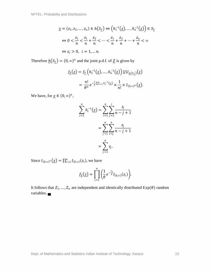
𝑧 = 𝑧1, 𝑧2, … , 𝑧𝑛 ∈ ℎ 𝑆𝑌 ⇔ ℎ1−1 𝑧 , … , ℎ𝑛

−1 𝑧 ∈ 𝑆𝑌

⇔ 0 <𝑧1

𝑛<

𝑧1

𝑛+

𝑧2

𝑛< ⋯ <

𝑧1

𝑛+

𝑧2

𝑛+ ⋯ +

𝑧𝑛

𝑛< ∞

⇔ 𝑧𝑖 > 0, 𝑖 = 1, …𝑛.

Therefore ℎ 𝑆𝑌 = 0,∞ 𝑛 and the joint p.d.f. of 𝑍 is given by

𝑓𝑍 𝑧 = 𝑓𝑌 ℎ1−1 𝑧 , … , ℎ𝑛

−1 𝑧 𝐽 𝐼ℎ 𝑆𝑌 𝑧

= 𝑛!

𝜃𝑛𝑒−

1

𝜃 ℎ𝑖

−1 𝑧 𝑛1=1 ×

1

𝑛!× 𝐼 0,∞ 𝑛 𝑧 .

We have, for 𝑧 ∈ 0,∞ 𝑛 ,

ℎ𝑖−1 𝑧

𝑛

𝑖=1

= 𝑧𝑗

𝑛 − 𝑗 + 1

𝑖

𝑗 =1

𝑛

𝑖=1

= 𝑧𝑗

𝑛 − 𝑗 + 1

𝑛

𝑖=𝑗

𝑛

𝑗 =1

= 𝑧𝑗

𝑛

𝑗 =1

.

Since 𝐼 0,∞ 𝑛 𝑧 = 𝐼 0,∞ 𝑧𝑖 𝑛𝑖=1 , we have

𝑓𝑍 𝑧 = 1

𝜃𝑒−

𝑧𝑖𝜃 𝐼 0,∞ 𝑧𝑖

𝑛

𝑖=1

.

It follows that 𝑍1, … , 𝑍𝑛 are independent and identically distributed Exp(𝜃) random

variables. ▄

Documents

Lecture34