Lecturenotes 4 MCMC I – Contents

1. Statistical Physics and Potts Models

2. Sampling and Re-weighting

3. Importance Sampling and Markov Chain Monte Carlo

4. The Metropolis Algorithm

5. The Heatbath Algorithm (Gibbs Sampler)

6. Start and Equilibration

7. Energy Checks

8. Specific Heat

1

Statistical Physics and Potts Model

MC simulations of systems described by the Gibbs canonical ensemble aim atcalculating estimators of physical observables at a temperature T . In the followingwe choose units so that β = 1/T and consider the calculation of the expectationvalue of an observable O. Mathematically all systems on a computer are discrete,because a finite word length has to be used. Hence,

O = O(β) = 〈O〉 = Z−1K∑

k=1

O(k) e−β E(k)(1)

where Z = Z(β) =K∑

k=1

e−β E(k)(2)

is the partition function. The index k = 1, . . . ,K labels all configurations (ormicrostates) of the system, and E(k) is the (internal) energy of configuration k.To distinguish the configuration index from other indices, it is put in parenthesis.

2

We introduce generalized Potts models in an external magnetic field on d-dimensional hypercubic lattices with periodic boundary conditions. Without beingoverly complicated, these models are general enough to illustrate the essentialfeatures we are interested in. In addition, various subcases of these models areby themselves of physical interest. Generalizations of the algorithmic concepts toother models are straightforward, although technical complications may arise.

We define the energy function of the system by

−β E(k) = −β E(k)0 + H M (k) (3)

where

E(k)0 = −2

∑〈ij〉

Jij(q(k)i , q

(k)j ) δ(q(k)

i , q(k)j ) +

2 d N

q(4)

with δ(qi, qj) ={

1 for qi = qj

0 for qi 6= qjand M (k) = 2

N∑i=1

δ(1, q(k)i ) .

3

The sum 〈ij〉 is over the nearest neighbor lattice sites and q(k)i is called the

Potts spin or Potts state of configuration k at site i. For the q-state Potts model

q(k)i takes on the values 1, . . . , q. The external magnetic field is chosen to interact

with the state qi = 1 at each site i, but not with the other states qi 6= 1. TheJij(qi, qj), (qi = 1, . . . , q; qj = 1, . . . , q) functions define the exchange couplingconstants between the states at site i and site j. The energy function describes anumber of physically interesting situations. With

Jij(qi, qj) ≡ J > 0 (conventionally J = 1) (5)

the original model is recovered and q = 2 becomes equivalent to the Isingferromagnet. The Ising case of Edwards-Anderson spin glasses and quadrupolarPotts glasses are obtained when the exchange constants are quenched randomvariables. Other choices of the Jij include anti-ferromagnets and the fully frustratedIsing model.

For the energy per spin the notation is: es = E/N .

4

The normalization is chosen so that es agrees for q = 2 with the conventionalIsing model definition, β = βIsing = βPotts/2 .

For the 2d Potts models a number of exact results are known in the infinitevolume limit, mainly due to work by Baxter. The phase transition temperatures are

12

βPottsc = βc =

1Tc

=12

ln(1 +√

q), q = 2, 3, . . . . (6)

At βc the average energy per state is

ec0s = Ec

0/N =4q− 2− 2/

√q . (7)

The phase transition is second order for q ≤ 4 and first order for q ≥ 5 for whichthe exact infinite volume latent heats 4e0s and entropy jumps 4s were also foundby Baxter, while the interface tensions fs were derived later.

5

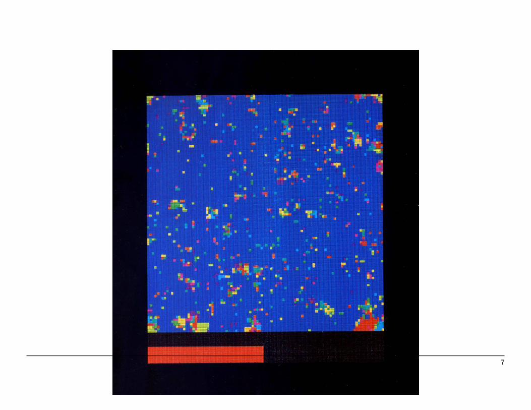
Some Potts Configurations (2d, q = 10)

1. Ordered with small fluctuations.

2. Disordered droplet in ordered background.

3. Percolated disordered phase (order-disorder separation)

6

7

8

9

Sampling and Re-weighting

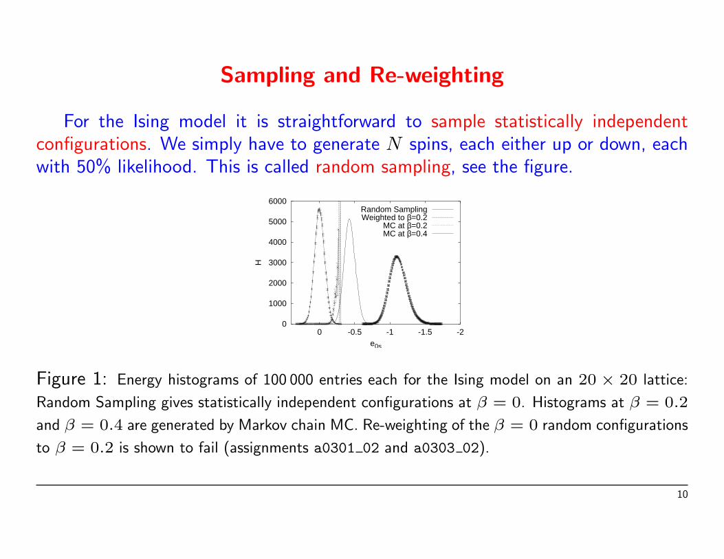
For the Ising model it is straightforward to sample statistically independentconfigurations. We simply have to generate N spins, each either up or down, eachwith 50% likelihood. This is called random sampling, see the figure.

0

1000

2000

3000

4000

5000

6000

-2-1.5-1-0.50

H

e0s

Random SamplingWeighted to β=0.2

MC at β=0.2MC at β=0.4

Figure 1: Energy histograms of 100 000 entries each for the Ising model on an 20 × 20 lattice:

Random Sampling gives statistically independent configurations at β = 0. Histograms at β = 0.2

and β = 0.4 are generated by Markov chain MC. Re-weighting of the β = 0 random configurations

to β = 0.2 is shown to fail (assignments a0301 02 and a0303 02).

10

Is is very important to distinguish the energy measurements es on singleconfigurations from the expectation value expectation value es. The expectationvalue es is a single number, while es fluctuates. From the measurement of manyes values one finds estimators of its moments. The mean is is denoted by es andfluctuates.

Histogram entries at β = 0 can be re-weighted, so that they correspond toother β values. We simply have to multiply the entry corresponding to energy E bycβ exp(−βE). Similarly histograms corresponding to the Gibbs ensemble at somevalue β0 can be re-weighted to other β values. (Care has to be taken to ensurethat the involved arguments of the exponential function do not become too large!This can be done by logarithmic coding.)

Re-weighting has a long history. For Finite Size Scaling (FSS) investigations ofsecond order phase transitions its usefulness has been stressed by Ferrenbergand Swendsen (accurate determinations of peaks of the specific heat or ofsusceptibilities).

11

In the figure re-weighting is done from β0 = 0 to β = 0.2. But, by comparisonto the histogram from a Metropolis MC calculation at β = 0.2, the result is seento be disastrous. The reason is easily identified: In the range where the β = 0.2histogram takes on its maximum, the β = 0 histogram has not a single entry,i.e., our naive sampling procedure misses the important configurations at β = 0.2.Re-weighting to new β values works only in a range β0 ±4β, where 4β → 0 inthe infinite volume limit.

Important Configurations

Let us determine the important contributions to the partition function. Thepartition function can be re-written as a sum over energies

Z = Z(β) =∑E

n(E) e−β E (8)

where the unnormalized spectral density n(E) is defined as the number ofmicrostates k with energy E (remember, on the computer energy values arealways discrete).

12

For a fixed value of β the energy probability density

Pβ(E) = cβ n(E) e−βE (9)

is peaked around the average value E(β), where cβ is a normalization constant sothat the

∑E Pβ(E) = 1 holds (consider the limits β = 0 and β →∞.)

Away from phase transitions the width of the energy distribution is 4E ∼√

V .This follows from the fact that, away from phase transition points, the fluctuationsof the N ∼ V lattice spins are essentially uncorrelated, so that the magnitude ofa typical fluctuations is ∼

√N . From this we find that the re-weighting range is

4β ∼ 1/√

V , as the energy is an extensive quantity ∼ V so that 4βE ∼√

V canstay within the fluctuation of the system.

Interestingly, the re-weighting range increases at second order phase transitions,because critical fluctuations are larger than non-critical fluctuations. Namely,one has 4E ∼ V x with 1/2 < x < 1 and the requirement 4βE ∼ V x yields4β ∼ V x−1.

13

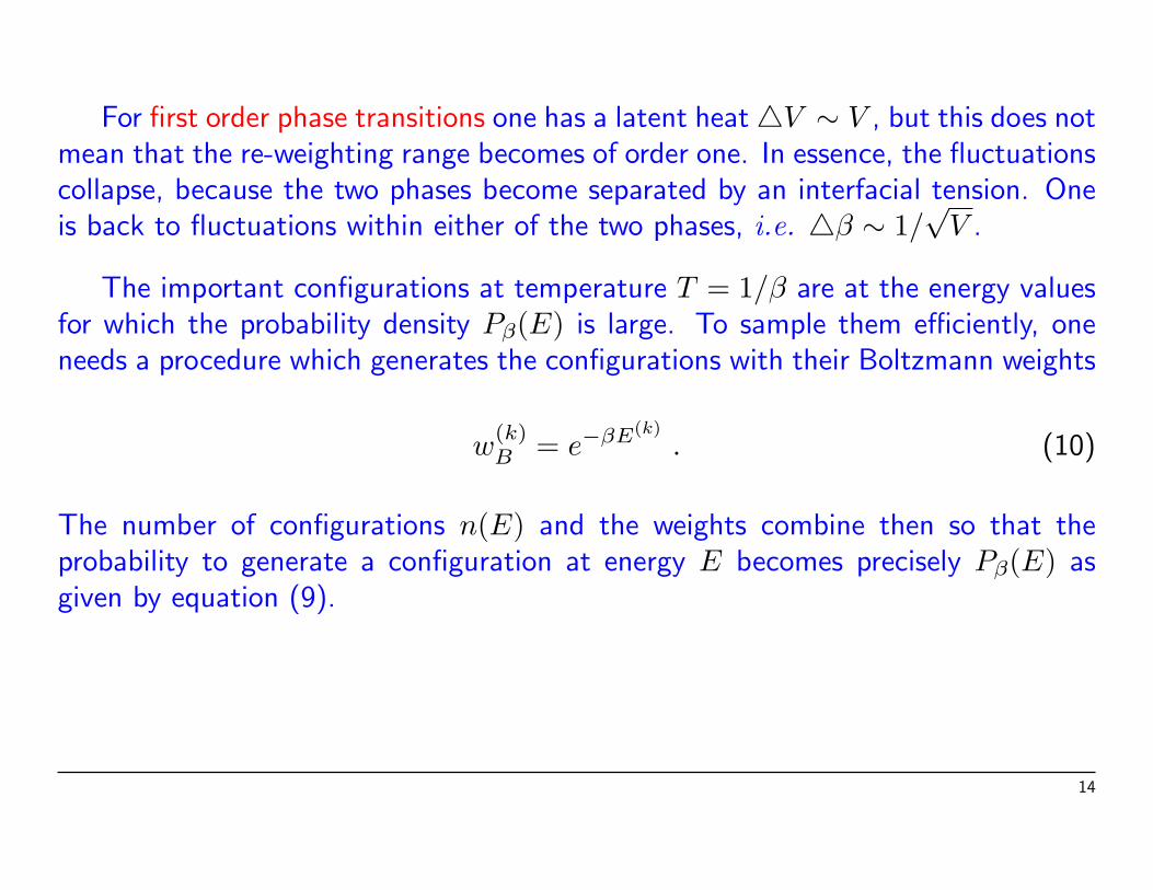
For first order phase transitions one has a latent heat4V ∼ V , but this does notmean that the re-weighting range becomes of order one. In essence, the fluctuationscollapse, because the two phases become separated by an interfacial tension. Oneis back to fluctuations within either of the two phases, i.e. 4β ∼ 1/

√V .

The important configurations at temperature T = 1/β are at the energy valuesfor which the probability density Pβ(E) is large. To sample them efficiently, oneneeds a procedure which generates the configurations with their Boltzmann weights

w(k)B = e−βE(k)

. (10)

The number of configurations n(E) and the weights combine then so that theprobability to generate a configuration at energy E becomes precisely Pβ(E) asgiven by equation (9).

14

Importance Sampling and Markov Chain Monte Carlo

For the canonical ensemble importance sampling generates configurations kwith probability

P(k)B = cB w

(k)B = cB e−βE(k)

, cB constant . (11)

The state vector (P (k)B ), for which the configurations are the vector indices, is

called Boltzmann state. The expectation value becomes the arithmetic average:

O = O(β) = 〈O〉 = limNK→∞

1NK

NK∑n=1

O(kn) . (12)

When the sum is truncated we obtain an estimator of the expectation value:

O =1

NK

NK∑k=1

O(kn) . (13)

15

Normally, we cannot generate configurations k directly with probability (11).But they may be found as members of the equilibrium distribution of adynamic process. In practice Markov chains are used. A Markov processis a particularly simple dynamic process, which generates configuration kn+1

stochastically from configuration kn, so that no information about previousconfigurations kn−1, kn−2, . . . is needed. The elements of the Markov chaintime series are the configurations. Assume that the configuration k is given. Letthe transition probability to create the configuration l in one step from k be givenby W (l)(k) = W [k → l]. In essence, the matrix

W =(W (l)(k)

)(14)

defines the Markov process. Note, that this transition matrix is a very big (neverstored in the computer!), because its labels are the configurations. To achieveour goal to generate configurations with the desired probabilities, the matrix W isrequired to satisfy the following properties:

16

(i) Ergodicity (Irreducibility in Math Literature):

e−βE(k)> 0 and e−βE(l)

> 0 imply : (15)

an integer number n > 0 exists so that (Wn)(l)(k) > 0 holds.

(ii) Normalization: ∑l

W (l)(k) = 1 . (16)

(iii) Balance (Stationarity):∑k

W (l)(k) e−βE(k)= e−βE(l)

. (17)

Balance means: The Boltzmann state (11) is an eigenvector with eigenvalue 1of the transition matrix W = (W (l)(k)).

17

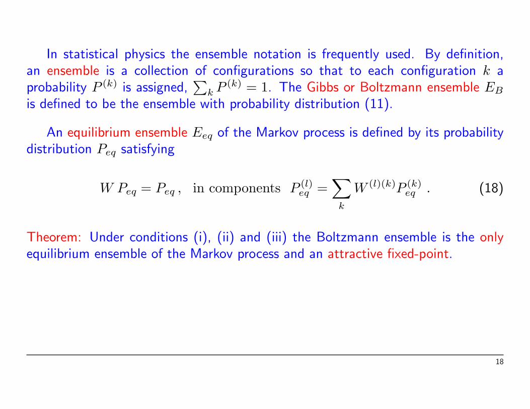
In statistical physics the ensemble notation is frequently used. By definition,an ensemble is a collection of configurations so that to each configuration k aprobability P (k) is assigned,

∑k P (k) = 1. The Gibbs or Boltzmann ensemble EB

is defined to be the ensemble with probability distribution (11).

An equilibrium ensemble Eeq of the Markov process is defined by its probabilitydistribution Peq satisfying

W Peq = Peq , in components P (l)eq =

∑k

W (l)(k)P (k)eq . (18)

Theorem: Under conditions (i), (ii) and (iii) the Boltzmann ensemble is the onlyequilibrium ensemble of the Markov process and an attractive fixed-point.

18

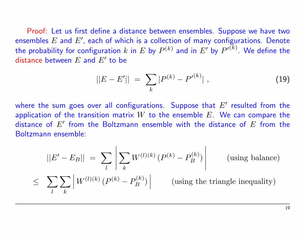
Proof: Let us first define a distance between ensembles. Suppose we have twoensembles E and E′, each of which is a collection of many configurations. Denote

the probability for configuration k in E by P (k) and in E′ by P ′(k). We define thedistance between E and E′ to be

||E − E′|| =∑

k

|P (k) − P ′(k)| , (19)

where the sum goes over all configurations. Suppose that E′ resulted from theapplication of the transition matrix W to the ensemble E. We can compare thedistance of E′ from the Boltzmann ensemble with the distance of E from theBoltzmann ensemble:

||E′ − EB|| =∑

l

∣∣∣∣∣ ∑k

W (l)(k) (P (k) − P(k)B )

∣∣∣∣∣ (using balance)

≤∑

l

∑k

∣∣∣ W (l)(k) (P (k) − P(k)B )

∣∣∣ (using the triangle inequality)

19

=∑

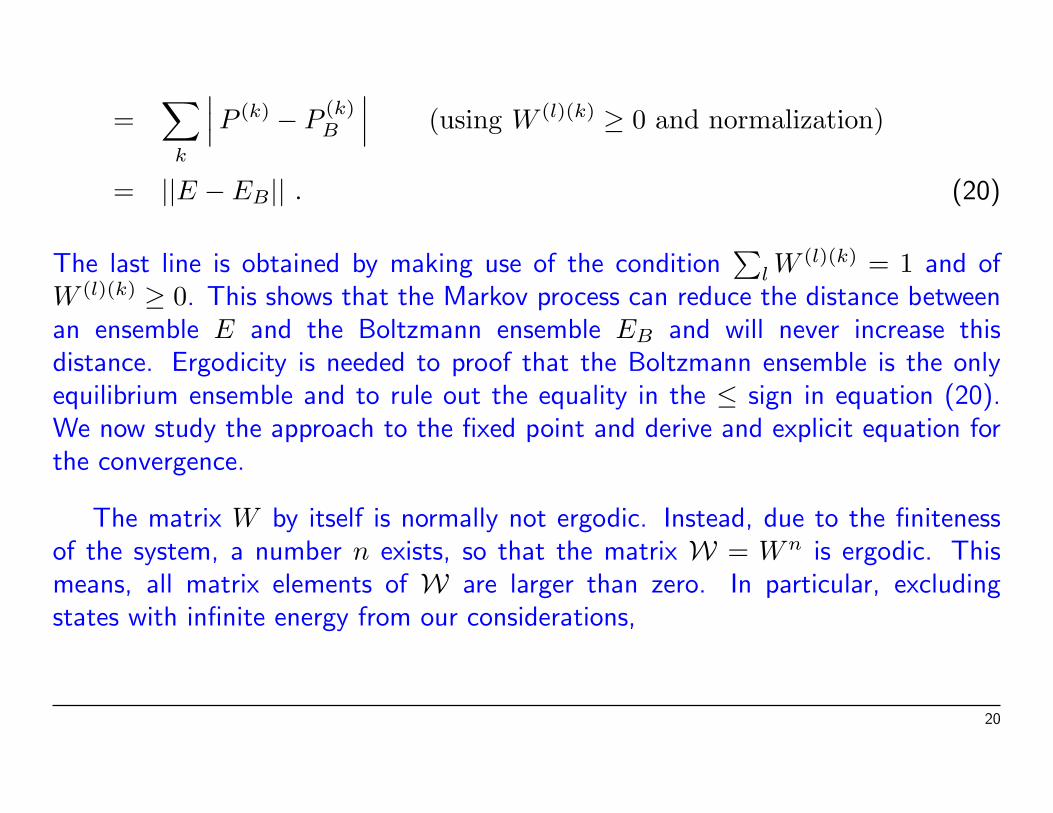
k

∣∣∣ P (k) − P(k)B

∣∣∣ (using W (l)(k) ≥ 0 and normalization)

= ||E − EB|| . (20)

The last line is obtained by making use of the condition∑

l W(l)(k) = 1 and of

W (l)(k) ≥ 0. This shows that the Markov process can reduce the distance betweenan ensemble E and the Boltzmann ensemble EB and will never increase thisdistance. Ergodicity is needed to proof that the Boltzmann ensemble is the onlyequilibrium ensemble and to rule out the equality in the ≤ sign in equation (20).We now study the approach to the fixed point and derive and explicit equation forthe convergence.

The matrix W by itself is normally not ergodic. Instead, due to the finitenessof the system, a number n exists, so that the matrix W = Wn is ergodic. Thismeans, all matrix elements of W are larger than zero. In particular, excludingstates with infinite energy from our considerations,

20

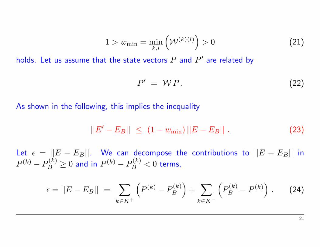
1 > wmin = mink,l

(W(k)(l)

)> 0 (21)

holds. Let us assume that the state vectors P and P ′ are related by

P ′ = W P . (22)

As shown in the following, this implies the inequality

||E′ − EB|| ≤ (1− wmin) ||E − EB|| . (23)

Let ε = ||E − EB||. We can decompose the contributions to ||E − EB|| in

P (k) − P(k)B ≥ 0 and in P (k) − P

(k)B < 0 terms,

ε = ||E − EB|| =∑

k∈K+

(P (k) − P

(k)B

)+

∑k∈K−

(P

(k)B − P (k)

). (24)

21

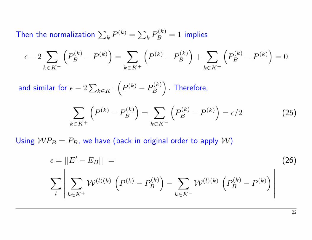
Then the normalization∑

k P (k) =∑

k P(k)B = 1 implies

ε− 2∑

k∈K−

(P

(k)B − P (k)

)=

∑k∈K+

(P (k) − P

(k)B

)+

∑k∈K+

(P

(k)B − P (k)

)= 0

and similar for ε− 2∑

k∈K+

(P (k) − P

(k)B

). Therefore,

∑k∈K+

(P (k) − P

(k)B

)=

∑k∈K−

(P

(k)B − P (k)

)= ε/2 (25)

Using WPB = PB, we have (back in original order to apply W)

ε = ||E′ − EB|| = (26)

∑l

∣∣∣∣∣∣∑

k∈K+

W(l)(k)(P (k) − P

(k)B

)−

∑k∈K−

W(l)(k)(P

(k)B − P (k)

) ∣∣∣∣∣∣22

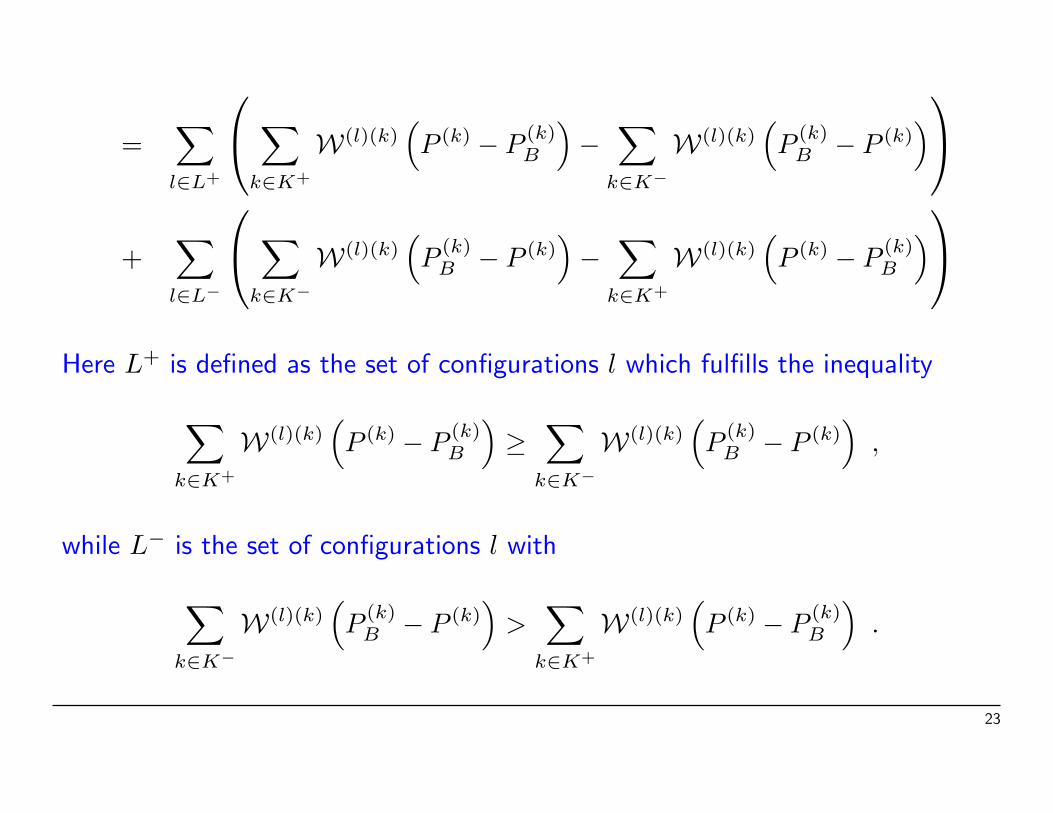
=∑l∈L+

∑k∈K+

W(l)(k)(P (k) − P

(k)B

)−

∑k∈K−

W(l)(k)(P

(k)B − P (k)

)+

∑l∈L−

∑k∈K−

W(l)(k)(P

(k)B − P (k)

)−

∑k∈K+

W(l)(k)(P (k) − P

(k)B

)Here L+ is defined as the set of configurations l which fulfills the inequality

∑k∈K+

W(l)(k)(P (k) − P

(k)B

)≥

∑k∈K−

W(l)(k)(P

(k)B − P (k)

),

while L− is the set of configurations l with

∑k∈K−

W(l)(k)(P

(k)B − P (k)

)>

∑k∈K+

W(l)(k)(P (k) − P

(k)B

).

23

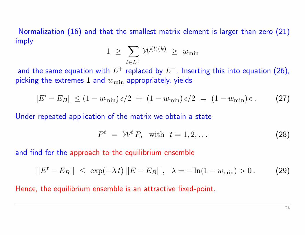
Normalization (16) and that the smallest matrix element is larger than zero (21)imply

1 ≥∑l∈L+

W(l)(k) ≥ wmin

and the same equation with L+ replaced by L−. Inserting this into equation (26),picking the extremes 1 and wmin appropriately, yields

||E′ − EB|| ≤ (1− wmin) ε/2 + (1− wmin) ε/2 = (1− wmin) ε . (27)

Under repeated application of the matrix we obtain a state

P t = Wt P, with t = 1, 2, . . . (28)

and find for the approach to the equilibrium ensemble

||Et − EB|| ≤ exp(−λ t) ||E − EB|| , λ = − ln(1− wmin) > 0 . (29)

Hence, the equilibrium ensemble is an attractive fixed-point.

24

There are many ways to construct a Markov process satisfying (i), (ii) and (iii).A stronger condition than balance (17) is

(iii’) Detailed balance:

W (l)(k) e−βE(k)= W (k)(l)e−βE(l)

. (30)

Using the normalization∑

k W (k)(l) = 1 detailed balance implies balance (iii).

At this point we have replaced the canonical ensemble average by a time average overan artificial dynamics. Calculating then averages over large times, like one does inreal experiments, is equivalent to calculating ensemble averages. One distinguishesdynamical universality classes. The Metropolis and heat bath algorithms discussedin the following fall into the class of model A or Glauber dynamics, which imitatesthe thermal fluctuations of nature to some extent. Cluster algorithms discussedconstitute another universality class. Some recent attention has focused ondynamical universality classes of non-equilibrium systems.

25

The Metropolis Algorithm

Detailed balance still does not uniquely fix the transition probabilities W (l)(k).The Metropolis algorithm can be used whenever one knows how to calculate theenergy of a configuration. Given a configuration k, the Metropolis algorithmproposes a configuration l with probability

f(l, k) normalized to∑

l

f(l, k) = 1 . (31)

For f(l, k) we derive a symmetry condition which ensures detailed balance. Thenew configuration l is accepted with probability

w(l)(k) = min

[1,

P(l)B

P(k)B

]=

{1 for E(l) < E(k)

e−β(E(l)−E(k)) for E(l) > E(k).(32)

If the new configuration is rejected, the old configuration has to be counted again.

26

The Metropolis procedure gives rise to the transition probabilities

W (l)(k) = f(l, k) w(l)(k) for l 6= k (33)

and W (k)(k) = f(k, k) +∑l 6=k

f(l, k) (1− w(l)(k)) . (34)

Therefore, the ratio(W (l)(k)/W (k)(l)

)satisfies detailed balance (30) if

f(l, k) = f(k, l) holds . (35)

Otherwise the probability density f(l, k) is unconstrained. So there is an amazingflexibility in the choice of the transition probabilities W (l)(k). One can even useacceptance probabilities distinct from those of equation (32) and the proposalprobabilities are then not necessarily symmetric anymore (Hastings). Also, thealgorithm generalizes immediately to arbitrary weights.

The acceptance rate is defined as the ratio of accepted changes over proposedmoves (moves proposing the at hand configuration are not counted as accepted).

27

Potts Model Heatbath Algorithm (Gibbs Sampler)

The heatbath algorithm chooses a state qi directly with the local Boltzmanndistribution defined by its nearest neighbors. The state qi can take on one of thevalues 1, . . . , q and, with all other states set, determines a value of the energyfunction. We denote this energy by E(qi) and the Boltzmann probabilities are

PB(qi) = const e−β E(qi) (36)

where the constant is determined by the normalization condition

q∑qi=1

PB(qi) = 1 . (37)

In equation (36) we can define E(qi) to be just the contribution of the interaction ofqi with its nearest neighbors to the total energy and absorb the other contributioninto the overall constant. The E(qi) values depend only on how the nearest

28

neighbors of the spin qi partition into the values 1, . . . , q. For low values of q andthe dimension d the most efficient implementation of the heatbath algorithm is totabulate all possibilities. However, here we prefer to give a generic code whichworks for arbitrary values of q and d.

For this we calculate the cumulative distribution function of the heat bathprobabilities

PHB(qi) =qi∑

q′i=1

PB(q′i) . (38)

The normalization condition (37) implies PHB(q) = 1. Comparison of thesecumulative probabilities with a uniform random number xr yields the heat bathupdate qi → q′i. Note that in the heat bath procedure the original value qin

i doesnot influence the selection of qnew

i .

29

Start and Equilibration

Initially we have to start with a microstate which may be far off the Boltzmanndistribution. Far off means, that the Boltzmann probability (at temperature T )for a typical state of the initially generated distribution can be very, very small.Suppression factors like 10−10000 are well possible. Although the weight of statesdecreases with 1/n where n is the steps of the Markov process, one should excludethe initial states from the equilibrium statistics. In practice this means we shouldallow for a certain number of sweeps nequi to equilibrate the system.

Many ways to generate start configurations exist. Two natural and easy toimplement choices are:

1. Generate a random configuration corresponding to β = 0. This defines a randomor disordered start of a MC simulation.

2. Generate a configuration for which all Potts spins take on the same q-value.This is called an ordered start of a MC simulation.

30

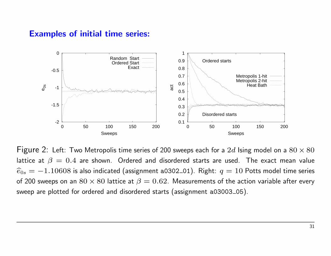
Examples of initial time series:

-2

-1.5

-1

-0.5

0

0 50 100 150 200

e 0s

Sweeps

Random StartOrdered Start

Exact

0.1

0.2

0.3

0.4

0.5

0.6

0.7

0.8

0.9

1

0 50 100 150 200

act

Sweeps

Ordered starts

Disordered starts

Metropolis 1-hitMetropolis 2-hit

Heat Bath

Figure 2: Left: Two Metropolis time series of 200 sweeps each for a 2d Ising model on a 80× 80

lattice at β = 0.4 are shown. Ordered and disordered starts are used. The exact mean valuebe0s = −1.10608 is also indicated (assignment a0302 01). Right: q = 10 Potts model time series

of 200 sweeps on an 80× 80 lattice at β = 0.62. Measurements of the action variable after every

sweep are plotted for ordered and disordered starts (assignment a03003 05).

31

Computer Program

program potts ts.f

subroutine potts init.f

subroutine lat init.f

subroutine potts act tab.f

subroutine potts order.f

subroutine potts ran.f

subroutine potts act.f

subroutine potts wght.f

subroutine potts met.f

32

Energy Checks

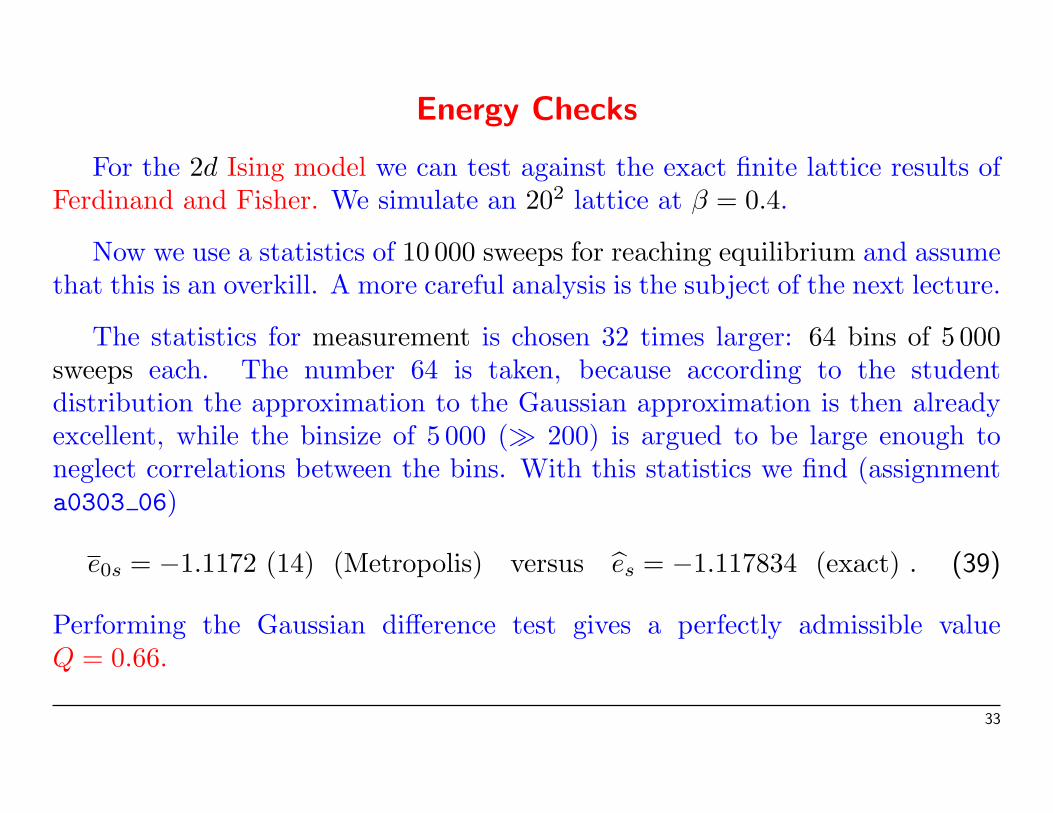
For the 2d Ising model we can test against the exact finite lattice results ofFerdinand and Fisher. We simulate an 202 lattice at β = 0.4.

Now we use a statistics of 10 000 sweeps for reaching equilibrium and assumethat this is an overkill. A more careful analysis is the subject of the next lecture.

The statistics for measurement is chosen 32 times larger: 64 bins of 5 000sweeps each. The number 64 is taken, because according to the studentdistribution the approximation to the Gaussian approximation is then alreadyexcellent, while the binsize of 5 000 (� 200) is argued to be large enough toneglect correlations between the bins. With this statistics we find (assignmenta0303 06)

e0s = −1.1172 (14) (Metropolis) versus es = −1.117834 (exact) . (39)

Performing the Gaussian difference test gives a perfectly admissible valueQ = 0.66.

33

Specific Heat

With E = 〈E〉 the specific heat is defined by

C =d E

d T= β2

(〈E2〉 − 〈E〉2

).

The last equal sign follows by working out the temperature derivative in thedefinition of the mean energy and is known as fluctuation-dissipation theorem.It is often used to estimate the specific heat from equilibrium simulationswithout relying on numerical derivatives. An equivalent formulation is

C = β2

⟨(E − E

)2⟩

as is easily shown by expanding(E − E

)2

and working out the expectation

34

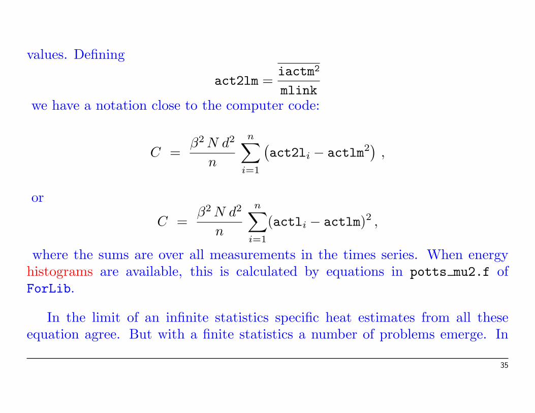
values. Defining

act2lm =iactm2

mlinkwe have a notation close to the computer code:

C =β2 N d2

n

n∑i=1

(act2li − actlm2

),

or

C =β2 N d2

n

n∑i=1

(actli − actlm)2 ,

where the sums are over all measurements in the times series. When energyhistograms are available, this is calculated by equations in potts mu2.f ofForLib.

In the limit of an infinite statistics specific heat estimates from all theseequation agree. But with a finite statistics a number of problems emerge. In

35

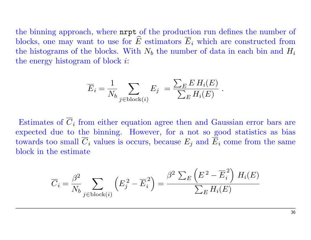
the binning approach, where nrpt of the production run defines the number ofblocks, one may want to use for E estimators Ei which are constructed fromthe histograms of the blocks. With Nb the number of data in each bin and Hi

the energy histogram of block i:

Ei =1

Nb

∑j∈block(i)

Ej =∑

E E Hi(E)∑E Hi(E)

.

Estimates of Ci from either equation agree then and Gaussian error bars areexpected due to the binning. However, for a not so good statistics as biastowards too small Ci values is occurs, because Ej and Ei come from the sameblock in the estimate

Ci =β2

Nb

∑j∈block(i)

(E 2

j − E2

i

)=

β2∑

E

(E 2 − E

2

i

)Hi(E)∑

E Hi(E)

36

=β2

Nb

∑j∈block(i)

(Ej − Ei

)2=

β2∑

E(E − Ei)2 Hi(E)∑E Hi(E)

.

The Ei estimators are certainly inferior to the estimate E, which relies on theentire statistics. Therefore, one may consider to use E instead of Ei. However,then one does not know anymore how to calculate the error bar of C as theCi estimates would rely on overlapping data. The situation gets even worsewhen we include reweighting, as this non-linear procedure implies that the twoestimators will in general differ. These difficulties are overcome by the jackknifemethod.

When histograms are used the fast way to create jackknife bins is to sumfirst the entire statistics:

H(E) =Nb∑i=1

Hi(E) .

37

Subsequently jackknife histograms (superscript J) are defined by

HJi (E) = H(E)−Hi(E)

and jackknife estimates CJ

i are obtained by using HJi (E) instead of Hi(E).

38