Embed Size (px)
Citation preview

Lecture Notes for Physics 110A
Daniel ArovasDepartment of Physics
University of California, San Diego
January 14, 2019

Contents
Contents i
List of Figures vii
1 Introduction to Dynamics 1
1.1 Introduction and Review . . . . . . . . . . . . . . . . . . . . . . . . . . . . . . . . . . . . 1
1.1.1 Newton’s laws of motion . . . . . . . . . . . . . . . . . . . . . . . . . . . . . . . . 1
1.1.2 Aside : inertial vs. gravitational mass . . . . . . . . . . . . . . . . . . . . . . . . . 3
1.2 Examples of Motion in One Dimension . . . . . . . . . . . . . . . . . . . . . . . . . . . . 4
1.2.1 Uniform force . . . . . . . . . . . . . . . . . . . . . . . . . . . . . . . . . . . . . . 4
1.2.2 Uniform force with linear frictional damping . . . . . . . . . . . . . . . . . . . . . 5
1.2.3 Uniform force with quadratic frictional damping . . . . . . . . . . . . . . . . . . . 6
1.2.4 Crossed electric and magnetic fields . . . . . . . . . . . . . . . . . . . . . . . . . . 7
1.3 Pause for Reflection . . . . . . . . . . . . . . . . . . . . . . . . . . . . . . . . . . . . . . . 8
2 Systems of Particles 9
2.1 Work-Energy Theorem . . . . . . . . . . . . . . . . . . . . . . . . . . . . . . . . . . . . . 9
2.2 Conservative and Nonconservative Forces . . . . . . . . . . . . . . . . . . . . . . . . . . . 10
2.2.1 Example : integrating F = −∇U . . . . . . . . . . . . . . . . . . . . . . . . . . . 12
2.3 Conservative Forces in Many Particle Systems . . . . . . . . . . . . . . . . . . . . . . . . 13
2.4 Linear and Angular Momentum . . . . . . . . . . . . . . . . . . . . . . . . . . . . . . . . 14
2.5 Scaling of Solutions for Homogeneous Potentials . . . . . . . . . . . . . . . . . . . . . . . 15
i
ii CONTENTS
2.5.1 Euler’s theorem for homogeneous functions . . . . . . . . . . . . . . . . . . . . . . 15
2.5.2 Scaled equations of motion . . . . . . . . . . . . . . . . . . . . . . . . . . . . . . . 16
2.6 Appendix I : Curvilinear Orthogonal Coordinates . . . . . . . . . . . . . . . . . . . . . . 17
2.6.1 Example : spherical coordinates . . . . . . . . . . . . . . . . . . . . . . . . . . . . 18
2.6.2 Vector calculus : grad, div, curl . . . . . . . . . . . . . . . . . . . . . . . . . . . . 19
2.7 Common curvilinear orthogonal systems . . . . . . . . . . . . . . . . . . . . . . . . . . . . 20
2.7.1 Rectangular coordinates . . . . . . . . . . . . . . . . . . . . . . . . . . . . . . . . 20
2.7.2 Cylindrical coordinates . . . . . . . . . . . . . . . . . . . . . . . . . . . . . . . . . 21
2.7.3 Spherical coordinates . . . . . . . . . . . . . . . . . . . . . . . . . . . . . . . . . . 22
2.7.4 Kinetic energy . . . . . . . . . . . . . . . . . . . . . . . . . . . . . . . . . . . . . . 23
3 One-Dimensional Conservative Systems 25
3.1 Description as a Dynamical System . . . . . . . . . . . . . . . . . . . . . . . . . . . . . . 25
3.1.1 Example : harmonic oscillator . . . . . . . . . . . . . . . . . . . . . . . . . . . . . 26
3.2 One-Dimensional Mechanics as a Dynamical System . . . . . . . . . . . . . . . . . . . . . 26
3.2.1 Sketching phase curves . . . . . . . . . . . . . . . . . . . . . . . . . . . . . . . . . 27
3.3 Fixed Points and their Vicinity . . . . . . . . . . . . . . . . . . . . . . . . . . . . . . . . . 28
3.3.1 Linearized dynamics in the vicinity of a fixed point . . . . . . . . . . . . . . . . . 29
3.4 Examples of Conservative One-Dimensional Systems . . . . . . . . . . . . . . . . . . . . . 31
3.4.1 Harmonic oscillator . . . . . . . . . . . . . . . . . . . . . . . . . . . . . . . . . . . 31
3.4.2 Pendulum . . . . . . . . . . . . . . . . . . . . . . . . . . . . . . . . . . . . . . . . 32
3.4.3 Other potentials . . . . . . . . . . . . . . . . . . . . . . . . . . . . . . . . . . . . . 33
4 Linear Oscillations 39
4.1 Damped Harmonic Oscillator . . . . . . . . . . . . . . . . . . . . . . . . . . . . . . . . . . 39
4.1.1 Classes of damped harmonic motion . . . . . . . . . . . . . . . . . . . . . . . . . . 40
4.1.2 Remarks on the case of critical damping . . . . . . . . . . . . . . . . . . . . . . . 42
4.1.3 Phase portraits for the damped harmonic oscillator . . . . . . . . . . . . . . . . . 44
4.2 Damped Harmonic Oscillator with Forcing . . . . . . . . . . . . . . . . . . . . . . . . . . 44

CONTENTS iii
4.2.1 Resonant forcing . . . . . . . . . . . . . . . . . . . . . . . . . . . . . . . . . . . . . 47
4.2.2 R-L-C circuits . . . . . . . . . . . . . . . . . . . . . . . . . . . . . . . . . . . . . . 47
4.2.3 Examples . . . . . . . . . . . . . . . . . . . . . . . . . . . . . . . . . . . . . . . . . 48
4.3 General solution by Green’s function method . . . . . . . . . . . . . . . . . . . . . . . . . 51
4.4 General Linear Autonomous Inhomogeneous ODEs . . . . . . . . . . . . . . . . . . . . . . 52
4.5 Kramers-Kronig Relations (advanced material) . . . . . . . . . . . . . . . . . . . . . . . . 56
5 Calculus of Variations 59
5.1 Snell’s Law . . . . . . . . . . . . . . . . . . . . . . . . . . . . . . . . . . . . . . . . . . . . 59
5.2 Functions and Functionals . . . . . . . . . . . . . . . . . . . . . . . . . . . . . . . . . . . . 60
5.2.1 Functional Taylor series . . . . . . . . . . . . . . . . . . . . . . . . . . . . . . . . . 64
5.3 Examples from the Calculus of Variations . . . . . . . . . . . . . . . . . . . . . . . . . . . 64
5.3.1 Example 1 : minimal surface of revolution . . . . . . . . . . . . . . . . . . . . . . 64
5.3.2 Example 2 : geodesic on a surface of revolution . . . . . . . . . . . . . . . . . . . 66
5.3.3 Example 3 : brachistochrone . . . . . . . . . . . . . . . . . . . . . . . . . . . . . . 67
5.3.4 Ocean waves . . . . . . . . . . . . . . . . . . . . . . . . . . . . . . . . . . . . . . . 68
5.4 Appendix : More on Functionals . . . . . . . . . . . . . . . . . . . . . . . . . . . . . . . . 70
6 Lagrangian Mechanics 77
6.1 Generalized Coordinates . . . . . . . . . . . . . . . . . . . . . . . . . . . . . . . . . . . . . 77
6.2 Hamilton’s Principle . . . . . . . . . . . . . . . . . . . . . . . . . . . . . . . . . . . . . . . 78
6.2.1 Invariance of the equations of motion . . . . . . . . . . . . . . . . . . . . . . . . . 78
6.2.2 Remarks on the order of the equations of motion . . . . . . . . . . . . . . . . . . 78
6.2.3 Lagrangian for a free particle . . . . . . . . . . . . . . . . . . . . . . . . . . . . . . 79
6.3 Conserved Quantities . . . . . . . . . . . . . . . . . . . . . . . . . . . . . . . . . . . . . . 80
6.3.1 Momentum conservation . . . . . . . . . . . . . . . . . . . . . . . . . . . . . . . . 80
6.3.2 Energy conservation . . . . . . . . . . . . . . . . . . . . . . . . . . . . . . . . . . . 81
6.4 Choosing Generalized Coordinates . . . . . . . . . . . . . . . . . . . . . . . . . . . . . . . 81
6.5 How to Solve Mechanics Problems . . . . . . . . . . . . . . . . . . . . . . . . . . . . . . . 82

iv CONTENTS
6.6 Examples . . . . . . . . . . . . . . . . . . . . . . . . . . . . . . . . . . . . . . . . . . . . . 83
6.6.1 One-dimensional motion . . . . . . . . . . . . . . . . . . . . . . . . . . . . . . . . 83
6.6.2 Central force in two dimensions . . . . . . . . . . . . . . . . . . . . . . . . . . . . 83
6.6.3 A sliding point mass on a sliding wedge . . . . . . . . . . . . . . . . . . . . . . . . 84
6.6.4 A pendulum attached to a mass on a spring . . . . . . . . . . . . . . . . . . . . . 85
6.6.5 The double pendulum . . . . . . . . . . . . . . . . . . . . . . . . . . . . . . . . . . 87
6.6.6 The thingy . . . . . . . . . . . . . . . . . . . . . . . . . . . . . . . . . . . . . . . . 89
6.7 Appendix : Virial Theorem . . . . . . . . . . . . . . . . . . . . . . . . . . . . . . . . . . . 91
7 Noether’s Theorem 93
7.1 Continuous Symmetry Implies Conserved Charges . . . . . . . . . . . . . . . . . . . . . . 93
7.1.1 Examples of one-parameter families of transformations . . . . . . . . . . . . . . . 94
7.1.2 Conservation of Linear and Angular Momentum . . . . . . . . . . . . . . . . . . . 95
7.1.3 Invariance of L vs. Invariance of S . . . . . . . . . . . . . . . . . . . . . . . . . . 96
7.2 The Hamiltonian . . . . . . . . . . . . . . . . . . . . . . . . . . . . . . . . . . . . . . . . . 97
7.2.1 Is H = T + U ? . . . . . . . . . . . . . . . . . . . . . . . . . . . . . . . . . . . . . 99
7.2.2 Example: A bead on a rotating hoop . . . . . . . . . . . . . . . . . . . . . . . . . 99
7.2.3 Charged Particle in a Magnetic Field . . . . . . . . . . . . . . . . . . . . . . . . . 102
7.3 Fast Perturbations : Rapidly Oscillating Fields . . . . . . . . . . . . . . . . . . . . . . . . 103
7.3.1 Example : pendulum with oscillating support . . . . . . . . . . . . . . . . . . . . 105
7.4 Field Theory: Systems with Several Independent Variables . . . . . . . . . . . . . . . . . 106
7.4.1 Gross-Pitaevskii model . . . . . . . . . . . . . . . . . . . . . . . . . . . . . . . . . 109
7.5 Hamiltonian Mechanics . . . . . . . . . . . . . . . . . . . . . . . . . . . . . . . . . . . . . 110
7.5.1 Modified Hamilton’s principle . . . . . . . . . . . . . . . . . . . . . . . . . . . . . 112
7.5.2 Phase flow is incompressible . . . . . . . . . . . . . . . . . . . . . . . . . . . . . . 112
7.5.3 Poincare recurrence theorem . . . . . . . . . . . . . . . . . . . . . . . . . . . . . . 112
7.5.4 Poisson brackets . . . . . . . . . . . . . . . . . . . . . . . . . . . . . . . . . . . . . 114
7.6 Canonical Transformations . . . . . . . . . . . . . . . . . . . . . . . . . . . . . . . . . . . 115
7.6.1 Point transformations in Lagrangian mechanics . . . . . . . . . . . . . . . . . . . 115
CONTENTS v
7.6.2 Canonical transformations in Hamiltonian mechanics . . . . . . . . . . . . . . . . 116
7.6.3 Hamiltonian evolution . . . . . . . . . . . . . . . . . . . . . . . . . . . . . . . . . 117
7.6.4 Symplectic structure . . . . . . . . . . . . . . . . . . . . . . . . . . . . . . . . . . 117
7.6.5 Generating functions for canonical transformations . . . . . . . . . . . . . . . . . 118
8 Constraints 121
8.1 Constraints and Variational Calculus . . . . . . . . . . . . . . . . . . . . . . . . . . . . . . 121
8.2 Constrained Extremization of Functions . . . . . . . . . . . . . . . . . . . . . . . . . . . . 123
8.3 Extremization of Functionals : Integral Constraints . . . . . . . . . . . . . . . . . . . . . 123
8.4 Extremization of Functionals : Holonomic Constraints . . . . . . . . . . . . . . . . . . . . 124
8.4.1 Examples of extremization with constraints . . . . . . . . . . . . . . . . . . . . . . 125
8.5 Application to Mechanics . . . . . . . . . . . . . . . . . . . . . . . . . . . . . . . . . . . . 127
8.5.1 Constraints and conservation laws . . . . . . . . . . . . . . . . . . . . . . . . . . . 128
8.6 Worked Examples . . . . . . . . . . . . . . . . . . . . . . . . . . . . . . . . . . . . . . . . 129
8.6.1 One cylinder rolling off another . . . . . . . . . . . . . . . . . . . . . . . . . . . . 129
8.6.2 Frictionless motion along a curve . . . . . . . . . . . . . . . . . . . . . . . . . . . 131
8.6.3 Disk rolling down an inclined plane . . . . . . . . . . . . . . . . . . . . . . . . . . 134
8.6.4 Pendulum with nonrigid support . . . . . . . . . . . . . . . . . . . . . . . . . . . . 135
8.6.5 Falling ladder . . . . . . . . . . . . . . . . . . . . . . . . . . . . . . . . . . . . . . 136
8.6.6 Point mass inside rolling hoop . . . . . . . . . . . . . . . . . . . . . . . . . . . . . 140
9 Central Forces and Orbital Mechanics 145
9.1 Reduction to a one-body problem . . . . . . . . . . . . . . . . . . . . . . . . . . . . . . . 145
9.1.1 Center-of-mass (CM) and relative coordinates . . . . . . . . . . . . . . . . . . . . 145
9.1.2 Solution to the CM problem . . . . . . . . . . . . . . . . . . . . . . . . . . . . . . 146
9.1.3 Solution to the relative coordinate problem . . . . . . . . . . . . . . . . . . . . . . 146
9.2 Almost Circular Orbits . . . . . . . . . . . . . . . . . . . . . . . . . . . . . . . . . . . . . 148
9.3 Precession in a Soluble Model . . . . . . . . . . . . . . . . . . . . . . . . . . . . . . . . . . 150
9.4 The Kepler Problem: U(r) = −k r−1 . . . . . . . . . . . . . . . . . . . . . . . . . . . . . . 152

vi CONTENTS
9.4.1 Geometric shape of orbits . . . . . . . . . . . . . . . . . . . . . . . . . . . . . . . 152
9.4.2 Laplace-Runge-Lenz vector . . . . . . . . . . . . . . . . . . . . . . . . . . . . . . . 152
9.4.3 Kepler orbits are conic sections . . . . . . . . . . . . . . . . . . . . . . . . . . . . 153
9.4.4 Period of bound Kepler orbits . . . . . . . . . . . . . . . . . . . . . . . . . . . . . 156
9.4.5 Escape velocity . . . . . . . . . . . . . . . . . . . . . . . . . . . . . . . . . . . . . 157
9.4.6 Satellites and spacecraft . . . . . . . . . . . . . . . . . . . . . . . . . . . . . . . . 157
9.4.7 Two examples of orbital mechanics . . . . . . . . . . . . . . . . . . . . . . . . . . 157
9.5 Appendix I : Mission to Neptune . . . . . . . . . . . . . . . . . . . . . . . . . . . . . . . . 160
9.5.1 I. Earth to Jupiter . . . . . . . . . . . . . . . . . . . . . . . . . . . . . . . . . . . 163
9.5.2 II. Encounter with Jupiter . . . . . . . . . . . . . . . . . . . . . . . . . . . . . . . 164
9.5.3 III. Jupiter to Neptune . . . . . . . . . . . . . . . . . . . . . . . . . . . . . . . . . 166
9.6 Appendix II : Restricted Three-Body Problem . . . . . . . . . . . . . . . . . . . . . . . . 167
10 Small Oscillations 173
10.1 Coupled Coordinates . . . . . . . . . . . . . . . . . . . . . . . . . . . . . . . . . . . . . . . 173
10.2 Expansion about Static Equilibrium . . . . . . . . . . . . . . . . . . . . . . . . . . . . . . 174
10.3 Method of Small Oscillations . . . . . . . . . . . . . . . . . . . . . . . . . . . . . . . . . . 174
10.3.1 Can you really just choose an A so that this works? . . . . . . . . . . . . . . . . . 175
10.3.2 Er...care to elaborate? . . . . . . . . . . . . . . . . . . . . . . . . . . . . . . . . . 175
10.3.3 Finding the modal matrix . . . . . . . . . . . . . . . . . . . . . . . . . . . . . . . 176
10.4 Example: Masses and Springs . . . . . . . . . . . . . . . . . . . . . . . . . . . . . . . . . . 177
10.5 Example: Double Pendulum . . . . . . . . . . . . . . . . . . . . . . . . . . . . . . . . . . 180
10.6 Zero Modes . . . . . . . . . . . . . . . . . . . . . . . . . . . . . . . . . . . . . . . . . . . . 181
10.6.1 Example of zero mode oscillations . . . . . . . . . . . . . . . . . . . . . . . . . . . 181
10.7 Chain of Mass Points . . . . . . . . . . . . . . . . . . . . . . . . . . . . . . . . . . . . . . 184
10.7.1 Continuum limit . . . . . . . . . . . . . . . . . . . . . . . . . . . . . . . . . . . . . 186
10.8 Appendix I : General Formulation . . . . . . . . . . . . . . . . . . . . . . . . . . . . . . . 188
10.9 Appendix II : Additional Examples . . . . . . . . . . . . . . . . . . . . . . . . . . . . . . 189
10.9.1 Right Triatomic Molecule . . . . . . . . . . . . . . . . . . . . . . . . . . . . . . . . 189

10.9.2 Triple Pendulum . . . . . . . . . . . . . . . . . . . . . . . . . . . . . . . . . . . . . 192
10.9.3 Equilateral Linear Triatomic Molecule . . . . . . . . . . . . . . . . . . . . . . . . 194
10.10 Aside : Christoffel Symbols . . . . . . . . . . . . . . . . . . . . . . . . . . . . . . . . . . . 198
11 Elastic Collisions 201
11.1 Center of Mass Frame . . . . . . . . . . . . . . . . . . . . . . . . . . . . . . . . . . . . . . 201
11.2 Central Force Scattering . . . . . . . . . . . . . . . . . . . . . . . . . . . . . . . . . . . . . 205
11.2.1 Hard sphere scattering . . . . . . . . . . . . . . . . . . . . . . . . . . . . . . . . . 207
11.2.2 Rutherford scattering . . . . . . . . . . . . . . . . . . . . . . . . . . . . . . . . . . 207
11.2.3 Transformation to laboratory coordinates . . . . . . . . . . . . . . . . . . . . . . . 208
List of Figures
2.1 Two paths joining points A and B. . . . . . . . . . . . . . . . . . . . . . . . . . . . . . . . 10
2.2 Volume element Ω for computing divergences. . . . . . . . . . . . . . . . . . . . . . . . . . 19
3.1 A potential U(x) and the corresponding phase portraits. . . . . . . . . . . . . . . . . . . . 28
3.2 Phase curves in the vicinity of centers and saddles. . . . . . . . . . . . . . . . . . . . . . . 30
3.3 Phase curves for the harmonic oscillator. . . . . . . . . . . . . . . . . . . . . . . . . . . . . 31
3.4 Phase curves for the simple pendulum. . . . . . . . . . . . . . . . . . . . . . . . . . . . . . 33
3.5 Phase curves for the Kepler effective potential U(x) = −x−1 + 12x
−2. . . . . . . . . . . . . 35
3.6 Phase curves for the potential U(x) = −sech2(x). . . . . . . . . . . . . . . . . . . . . . . . 36
3.7 Phase curves for the potential U(x) = cos(x) + 12x. . . . . . . . . . . . . . . . . . . . . . . 37
4.1 Three classifications of damped harmonic motion . . . . . . . . . . . . . . . . . . . . . . . 41
4.2 Phase curves for the damped harmonic oscillator . . . . . . . . . . . . . . . . . . . . . . . 43
4.3 Amplitude and phase shift versus oscillator frequency . . . . . . . . . . . . . . . . . . . . 46
vii

viii LIST OF FIGURES
4.4 An R-L-C circuit which behaves as a damped harmonic oscillator . . . . . . . . . . . . . . 48
4.5 A driven L-C-R circuit, with V (t) = V0 cos(ωt) . . . . . . . . . . . . . . . . . . . . . . . . 49
4.6 The equivalent mechanical circuit for fig. 4.5 . . . . . . . . . . . . . . . . . . . . . . . . . 50
4.7 Response of an underdamped oscillator to a pulse force . . . . . . . . . . . . . . . . . . . 53
5.1 The shortest path between two points . . . . . . . . . . . . . . . . . . . . . . . . . . . . . 60
5.2 The path of shortest length is composed of three line segments . . . . . . . . . . . . . . . 61
5.3 A path y(x) and its variation y(x) + δy(x) . . . . . . . . . . . . . . . . . . . . . . . . . . . 62
5.4 Minimal surface solution . . . . . . . . . . . . . . . . . . . . . . . . . . . . . . . . . . . . . 65
5.5 Breaking of shallow water waves . . . . . . . . . . . . . . . . . . . . . . . . . . . . . . . . 69
5.6 A functional as a continuum limit of a multivariable function. . . . . . . . . . . . . . . . . 71
6.1 A mass sliding down a wedge. . . . . . . . . . . . . . . . . . . . . . . . . . . . . . . . . . . 84
6.2 The spring–pendulum system . . . . . . . . . . . . . . . . . . . . . . . . . . . . . . . . . . 85
6.3 The double pendulum . . . . . . . . . . . . . . . . . . . . . . . . . . . . . . . . . . . . . . 87
6.4 The thingy . . . . . . . . . . . . . . . . . . . . . . . . . . . . . . . . . . . . . . . . . . . . 90
7.1 A bead of mass m on a rotating hoop of radius a . . . . . . . . . . . . . . . . . . . . . . . 100
7.2 The effective potential Ueff(θ) . . . . . . . . . . . . . . . . . . . . . . . . . . . . . . . . . . 101
7.3 Dimensionless potential v(θ) . . . . . . . . . . . . . . . . . . . . . . . . . . . . . . . . . . . 106
8.1 A cylinder of radius a rolls along a half-cylinder of radius R . . . . . . . . . . . . . . . . . 122
8.2 Frictionless motion under gravity along a curved surface . . . . . . . . . . . . . . . . . . . 131
8.3 Finding the local radius of curvature: z = η2/2R . . . . . . . . . . . . . . . . . . . . . . . 133
8.4 A hoop rolling down an inclined plane lying on a frictionless surface . . . . . . . . . . . . 134
8.5 A ladder sliding down a wall and across a floor . . . . . . . . . . . . . . . . . . . . . . . . 137
8.6 Plot of time to fall for the slipping ladder . . . . . . . . . . . . . . . . . . . . . . . . . . . 139
8.7 A point mass inside a hoop . . . . . . . . . . . . . . . . . . . . . . . . . . . . . . . . . . . 141
9.1 Center-of-mass (R) and relative (r) coordinates . . . . . . . . . . . . . . . . . . . . . . . . 146
9.2 Stable and unstable circular orbits . . . . . . . . . . . . . . . . . . . . . . . . . . . . . . . 149

LIST OF FIGURES ix
9.3 Precession in a soluble model . . . . . . . . . . . . . . . . . . . . . . . . . . . . . . . . . . 151
9.4 The effective potential and phase curves for the Kepler problem . . . . . . . . . . . . . . . 152
9.5 Keplerian orbits are conic sections . . . . . . . . . . . . . . . . . . . . . . . . . . . . . . . 154
9.6 The Keplerian ellipse, with the force center at the left focus . . . . . . . . . . . . . . . . . 155
9.7 The Keplerian hyperbolae, with the force center at the left focus . . . . . . . . . . . . . . 156
9.8 At perigee of an elliptical orbit ri(φ), a radial impulse ∆p is applied . . . . . . . . . . . . 158
9.9 Two Keplerian orbits about the sun . . . . . . . . . . . . . . . . . . . . . . . . . . . . . . 159
9.10 The unforgivably dorky Pioneer 10 and Pioneer 11 plaque . . . . . . . . . . . . . . . . . 161
9.11 Mission to Neptune . . . . . . . . . . . . . . . . . . . . . . . . . . . . . . . . . . . . . . . . 162
9.12 Total time for Earth-Neptune mission as a function of dimensionless velocity at perihelion 166
9.13 The Lagrange points for the earth-sun system . . . . . . . . . . . . . . . . . . . . . . . . . 168
9.14 Graphical solution for the Lagrange points L1, L2, and L3 . . . . . . . . . . . . . . . . . . 170
10.1 A system of masses and springs . . . . . . . . . . . . . . . . . . . . . . . . . . . . . . . . . 178
10.2 The double pendulum . . . . . . . . . . . . . . . . . . . . . . . . . . . . . . . . . . . . . . 180
10.3 Coupled oscillations of three masses on a frictionless hoop . . . . . . . . . . . . . . . . . . 182
10.4 Normal modes of the 45 right triangle . . . . . . . . . . . . . . . . . . . . . . . . . . . . . 191
10.5 The triple pendulum . . . . . . . . . . . . . . . . . . . . . . . . . . . . . . . . . . . . . . . 192
10.6 An equilateral triangle of identical mass points and springs . . . . . . . . . . . . . . . . . 195
10.7 Zero modes of the mass-spring triangle . . . . . . . . . . . . . . . . . . . . . . . . . . . . . 196
10.8 Finite oscillation frequency modes of the mass-spring triangle . . . . . . . . . . . . . . . . 197
10.9 John Henry . . . . . . . . . . . . . . . . . . . . . . . . . . . . . . . . . . . . . . . . . . . . 198
11.1 The scattering of two hard spheres of radii a and b . . . . . . . . . . . . . . . . . . . . . . 202
11.2 Scattering of two particles of masses m1 and m2 . . . . . . . . . . . . . . . . . . . . . . . 203
11.3 Scattering when particle 2 is initially at rest . . . . . . . . . . . . . . . . . . . . . . . . . . 204
11.4 Scattering of identical mass particles when particle 2 is initially at rest . . . . . . . . . . . 204
11.5 Repulsive and attractive scattering in the lab and CM frames . . . . . . . . . . . . . . . . 205
11.6 Scattering in the CM frame . . . . . . . . . . . . . . . . . . . . . . . . . . . . . . . . . . . 206
11.7 Geometry of hard sphere scattering . . . . . . . . . . . . . . . . . . . . . . . . . . . . . . . 207

x LIST OF FIGURES

Chapter 1
Introduction to Dynamics
1.1 Introduction and Review
Dynamics is the science of how things move. A complete solution to the motion of a system means thatwe know the coordinates of all its constituent particles as functions of time. For a single point particlemoving in three-dimensional space, this means we want to know its position vector r(t) as a function of
time. If there are many particles, the motion is described by a set of functions ri(t), where i labels whichparticle we are talking about. So generally speaking, solving for the motion means being able to predictwhere a particle will be at any given instant of time. Of course, knowing the function ri(t) means we can
take its derivative and obtain the velocity vi(t) = dri/dt at any time as well.
The complete motion for a system is not given to us outright, but rather is encoded in a set of differentialequations, called the equations of motion. An example of an equation of motion is
md2x
dt2= −mg (1.1)
with the solutionx(t) = x0 + v0t− 1
2gt2 (1.2)
where x0 and v0 are constants corresponding to the initial boundary conditions on the position andvelocity: x(0) = x0, v(0) = v0. This particular solution describes the vertical motion of a particle of massm moving near the earth’s surface.
In this class, we shall discuss a general framework by which the equations of motion may be obtained,and methods for solving them. That “general framework” is Lagrangian Dynamics, which itself is reallynothing more than an elegant restatement of Isaac Newton’s Laws of Motion.
1.1.1 Newton’s laws of motion
Aristotle held that objects move because they are somehow impelled to seek out their natural state.Thus, a rock falls because rocks belong on the earth, and flames rise because fire belongs in the heavens.
1

2 CHAPTER 1. INTRODUCTION TO DYNAMICS
To paraphrase Wolfgang Pauli, such notions are so vague as to be “not even wrong.” It was only with thepublication of Newton’s Principia in 1687 that a theory of motion which had detailed predictive powerwas developed.
Newton’s three Laws of Motion may be stated as follows:
I. A body remains in uniform motion unless acted on by a force.
II. Force equals rate of change of momentum: F = dp/dt.
III. Any two bodies exert equal and opposite forces on each other.
Newton’s First Law states that a particle will move in a straight line at constant (possibly zero) velocityif it is subjected to no forces. Now this cannot be true in general, for suppose we encounter such a “free”particle and that indeed it is in uniform motion, so that r(t) = r0 + v0t. Now r(t) is measured in somecoordinate system, and if instead we choose to measure r(t) in a different coordinate system whose originR moves according to the function R(t), then in this new “frame of reference” the position of our particlewill be
r′(t) = r(t)−R(t)
= r0 + v0t−R(t) .
If the acceleration d2R/dt2 is nonzero, then merely by shifting our frame of reference we have apparentlyfalsified Newton’s First Law – a free particle does not move in uniform rectilinear motion when viewedfrom an accelerating frame of reference. Thus, together with Newton’s Laws comes an assumptionabout the existence of frames of reference – called inertial frames – in which Newton’s Laws hold. Atransformation from one frame K to another frame K′ which moves at constant velocity V relative to Kis called a Galilean transformation. The equations of motion of classical mechanics are invariant (do notchange) under Galilean transformations.
At first, the issue of inertial and noninertial frames is confusing. Rather than grapple with this, we willtry to build some intuition by solving mechanics problems assuming we are in an inertial frame. Theearth’s surface, where most physics experiments are done, is not an inertial frame, due to the centripetalaccelerations associated with the earth’s rotation about its own axis and its orbit around the sun. Inthis case, not only is our coordinate system’s origin – somewhere in a laboratory on the surface of theearth – accelerating, but the coordinate axes themselves are rotating with respect to an inertial frame.The rotation of the earth leads to fictitious “forces” such as the Coriolis force, which have large-scaleconsequences. For example, hurricanes, when viewed from above, rotate counterclockwise in the northernhemisphere and clockwise in the southern hemisphere. Later on in the course we will devote ourselves toa detailed study of motion in accelerated coordinate systems.
Newton’s “quantity of motion” is the momentum p, defined as the product p = mv of a particle’s massm (how much stuff there is) and its velocity (how fast it is moving). In order to convert the SecondLaw into a meaningful equation, we must know how the force F depends on the coordinates (or possibly

1.1. INTRODUCTION AND REVIEW 3
velocities) themselves. This is known as a force law. Examples of force laws include:
Constant force: F = −mg
Hooke’s Law: F = −kx
Gravitation: F = −GMm r/r2
Lorentz force: F = qE + qv
c×B
Fluid friction (v small): F = −bv .
Note that for an object whose mass does not change we can write the Second Law in the familiar formF = ma, where a = dv/dt = d2r/dt2 is the acceleration. Most of our initial efforts will lie in usingNewton’s Second Law to solve for the motion of a variety of systems.
The Third Law is valid for the extremely important case of central forces which we will discuss in greatdetail later on. Newtonian gravity – the force which makes the planets orbit the sun – is a central force.One consequence of the Third Law is that in free space two isolated particles will accelerate in such away that F1 = −F2 and hence the accelerations are parallel to each other, with
a1a2
= −m2
m1, (1.3)
where the minus sign is used here to emphasize that the accelerations are in opposite directions. We canalso conclude that the total momentum P = p1 + p2 is a constant, a result known as the conservation of
momentum.
1.1.2 Aside : inertial vs. gravitational mass
In addition to postulating the Laws of Motion, Newton also deduced the gravitational force law, whichsays that the force Fij exerted by a particle i by another particle j is
Fij = −Gmimj
ri − rj|ri − rj |3
, (1.4)
where G, the Cavendish constant (first measured by Henry Cavendish in 1798), takes the value
G = (6.6726 ± 0.0008) × 10−11N ·m2/kg2 . (1.5)
Notice Newton’s Third Law in action: Fij + Fji = 0. Now a very important and special feature of this“inverse square law” force is that a spherically symmetric mass distribution has the same force on anexternal body as it would if all its mass were concentrated at its center. Thus, for a particle of mass mnear the surface of the earth, we can take mi = m and mj =Me, with ri − rj ≃ Rer and obtain
F = −mgr ≡ −mg (1.6)
4 CHAPTER 1. INTRODUCTION TO DYNAMICS
where r is a radial unit vector pointing from the earth’s center and g = GMe/R2e ≃ 9.8m/s2 is the
acceleration due to gravity at the earth’s surface. Newton’s Second Law now says that a = −g, i.e.objects accelerate as they fall to earth. However, it is not a priori clear why the inertial mass whichenters into the definition of momentum should be the same as the gravitational mass which enters intothe force law. Suppose, for instance, that the gravitational mass took a different value, m′. In this case,Newton’s Second Law would predict
a = −m′
mg (1.7)
and unless the ratio m′/m were the same number for all objects, then bodies would fall with different
accelerations. The experimental fact that bodies in a vacuum fall to earth at the same rate demonstratesthe equivalence of inertial and gravitational mass, i.e. m′ = m.
1.2 Examples of Motion in One Dimension
To gain some experience with solving equations of motion in a physical setting, we consider some physicallyrelevant examples of one-dimensional motion.
1.2.1 Uniform force
With F = −mg, appropriate for a particle falling under the influence of a uniform gravitational field, wehave md2x/dt2 = −mg, or x = −g. Notation:
x ≡ dx
dt, x ≡ d2x
dt2,
˙x =
d7x
dt7, etc. (1.8)
With v = x, we solve dv/dt = −g:v(t)∫
v(0)
dv =
t∫
0
ds (−g)
v(t)− v(0) = −gt .
(1.9)
Note that there is a constant of integration, v(0), which enters our solution.
We are now in position to solve dx/dt = v:
x(t)∫
x(0)
dx =
t∫
0
ds v(s)
x(t) = x(0) +
t∫
0
ds[v(0)− gs
]
= x(0) + v(0)t − 12gt
2 .
(1.10)
Note that a second constant of integration, x(0), has appeared.

1.2. EXAMPLES OF MOTION IN ONE DIMENSION 5
1.2.2 Uniform force with linear frictional damping
In this case,
mdv
dt= −mg − γv (1.11)
which may be rewritten
dv
v +mg/γ= − γ
mdt
d ln(v +mg/γ) = −(γ/m)dt .
(1.12)
Integrating then gives
ln
(v(t) +mg/γ
v(0) +mg/γ
)= −γt/m
v(t) = −mgγ
+
(v(0) +
mg
γ
)e−γt/m .
(1.13)
Note that the solution to the first order ODE mv = −mg − γv entails one constant of integration, v(0).
One can further integrate to obtain the motion
x(t) = x(0) +m
γ
(v(0) +
mg
γ
)(1− e−γt/m)− mg
γt . (1.14)
The solution to the second order ODE mx = −mg − γx thus entails two constants of integration: v(0)
and x(0). Notice that as t goes to infinity the velocity tends towards the asymptotic value v = −v∞,
where v∞ = mg/γ. This is known as the terminal velocity. Indeed, solving the equation v = 0 gives
v = −v∞. The initial velocity is effectively “forgotten” on a time scale τ ≡ m/γ.
Electrons moving in solids under the influence of an electric field also achieve a terminal velocity. In thiscase the force is not F = −mg but rather F = −eE, where −e is the electron charge (e > 0) and E isthe electric field. The terminal velocity is then obtained from
v∞ = eE/γ = eτE/m . (1.15)
The current density is a product:
current density = (number density)× (charge) × (velocity)
j = n · (−e) · (−v∞)
=ne2τ
mE .
(1.16)
The ratio j/E is called the conductivity of the metal, σ. According to our theory, σ = ne2τ/m. This isone of the most famous equations of solid state physics! The dissipation is caused by electrons scatteringoff impurities and lattice vibrations (“phonons”). In high purity copper at low temperatures (T <∼ 4K),the scattering time τ is about a nanosecond (τ ≈ 10−9 s).

6 CHAPTER 1. INTRODUCTION TO DYNAMICS
1.2.3 Uniform force with quadratic frictional damping
At higher velocities, the frictional damping is proportional to the square of the velocity. The frictionalforce is then Ff = −cv2 sgn (v), where sgn (v) is the sign of v: sgn (v) = +1 if v > 0 and sgn (v) = −1if v < 0. (Note one can also write sgn (v) = v/|v| where |v| is the absolute value.) Why all this troublewith sgn (v)? Because it is important that the frictional force dissipate energy, and therefore that Ff beoppositely directed with respect to the velocity v. We will assume that v < 0 always, hence Ff = +cv2.
Notice that there is a terminal velocity, since setting v = −g + (c/m)v2 = 0 gives v = ±v∞, where
v∞ =√mg/c. One can write the equation of motion as
dv
dt=
g
v2∞(v2 − v2∞) (1.17)
and using1
v2 − v2∞=
1
2v∞
[1
v − v∞− 1
v + v∞
](1.18)
we obtain
dv
v2 − v2∞=
1
2v∞
dv
v − v∞− 1
2v∞
dv
v + v∞
=1
2v∞d ln
(v∞ − v
v∞ + v
)
=g
v2∞dt .
(1.19)
Assuming v(0) = 0, we integrate to obtain
1
2v∞ln
(v∞ − v(t)
v∞ + v(t)
)=
gt
v2∞(1.20)
which may be massaged to give the final result
v(t) = −v∞ tanh(gt/v∞) . (1.21)
Recall that the hyperbolic tangent function tanh(x) is given by
tanh(x) =sinh(x)
cosh(x)=ex − e−x
ex + e−x. (1.22)
Again, as t→ ∞ one has v(t) → −v∞, i.e. v(∞) = −v∞.
Advanced Digression: To gain an understanding of the constant c, consider a flat surface of area Smoving through a fluid at velocity v (v > 0). During a time ∆t, all the fluid molecules inside the volume∆V = S · v∆t will have executed an elastic collision with the moving surface. Since the surface isassumed to be much more massive than each fluid molecule, the center of mass frame for the surface-molecule collision is essentially the frame of the surface itself. If a molecule moves with velocity u is thelaboratory frame, it moves with velocity u− v in the center of mass (CM) frame, and since the collisionis elastic, its final CM frame velocity is reversed, to v − u. Thus, in the laboratory frame the molecule’s
1.2. EXAMPLES OF MOTION IN ONE DIMENSION 7
velocity has become 2v−u and it has suffered a change in velocity of ∆u = 2(v−u). The total momentumchange is obtained by multiplying ∆u by the total mass M = ∆V , where is the mass density of thefluid. But then the total momentum imparted to the fluid is
∆P = 2(v − u) · S v∆t (1.23)
and the force on the fluid is
F =∆P
∆t= 2S v(v − u) . (1.24)
Now it is appropriate to average this expression over the microscopic distribution of molecular velocitiesu, and since on average 〈u〉 = 0, we obtain the result 〈F 〉 = 2Sv2, where 〈· · · 〉 denotes a microscopicaverage over the molecular velocities in the fluid. (There is a subtlety here concerning the effect offluid molecules striking the surface from either side – you should satisfy yourself that this derivation issensible!) Newton’s Third Law then states that the frictional force imparted to the moving surface bythe fluid is Ff = −〈F 〉 = −cv2, where c = 2S. In fact, our derivation is too crude to properly obtainthe numerical prefactors, and it is better to write c = µS, where µ is a dimensionless constant whichdepends on the shape of the moving object.
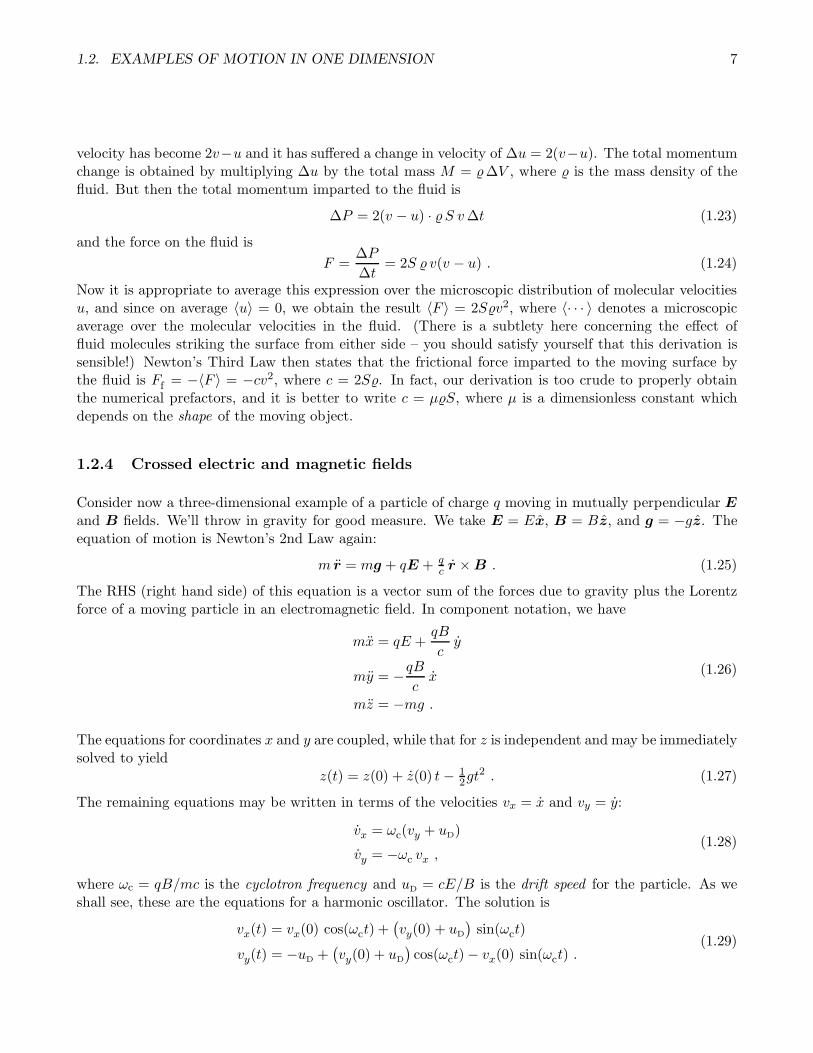
1.2.4 Crossed electric and magnetic fields
Consider now a three-dimensional example of a particle of charge q moving in mutually perpendicular Eand B fields. We’ll throw in gravity for good measure. We take E = Ex, B = Bz, and g = −gz. Theequation of motion is Newton’s 2nd Law again:
m r = mg + qE + qc r ×B . (1.25)
The RHS (right hand side) of this equation is a vector sum of the forces due to gravity plus the Lorentzforce of a moving particle in an electromagnetic field. In component notation, we have
mx = qE +qB
cy
my = −qBcx
mz = −mg .
(1.26)
The equations for coordinates x and y are coupled, while that for z is independent and may be immediatelysolved to yield
z(t) = z(0) + z(0) t− 12gt
2 . (1.27)
The remaining equations may be written in terms of the velocities vx = x and vy = y:
vx = ωc(vy + uD)
vy = −ωc vx ,(1.28)
where ωc = qB/mc is the cyclotron frequency and uD = cE/B is the drift speed for the particle. As weshall see, these are the equations for a harmonic oscillator. The solution is
vx(t) = vx(0) cos(ωct) +(vy(0) + uD
)sin(ωct)
vy(t) = −uD +(vy(0) + uD
)cos(ωct)− vx(0) sin(ωct) .
(1.29)

8 CHAPTER 1. INTRODUCTION TO DYNAMICS
Integrating again, the full motion is given by:
x(t) = x(0) +A sin δ +A sin(ωct− δ)
y(r) = y(0)− uD t−A cos δ +A cos(ωct− δ) ,(1.30)
where
A =1
ωc
√x2(0) +
(y(0) + uD
)2, δ = tan−1
(y(0) + uD
x(0)
). (1.31)
Thus, in the full solution of the motion there are six constants of integration:
x(0) , y(0) , z(0) , A , δ , z(0) . (1.32)
Of course instead of A and δ one may choose as constants of integration x(0) and y(0).
1.3 Pause for Reflection
In mechanical systems, for each coordinate, or “degree of freedom,” there exists a corresponding secondorder ODE. The full solution of the motion of the system entails two constants of integration for eachdegree of freedom.

Chapter 2
Systems of Particles
2.1 Work-Energy Theorem
Consider a system of many particles, with positions ri and velocities ri. The kinetic energy of this systemis
T =∑
i
Ti =∑
i
12mir
2i . (2.1)
Now let’s consider how the kinetic energy of the system changes in time. Assuming each mi is time-independent, we have
dTidt
= mi ri · ri . (2.2)
Here, we’ve used the relationd
dt
(A2)= 2A · dA
dt. (2.3)
We now invoke Newton’s 2nd Law, miri = Fi, to write eqn. 2.2 as Ti = Fi · ri. We integrate this equation
from time tA to tB:
T (B)
i − T (A)
i =
tB∫
tA
dtdTidt
=
tB∫
tA
dtFi · ri ≡∑
i
W (A→B)
i ,
(2.4)
where W (A→B)
i is the total work done on particle i during its motion from state A to state B, Clearly thetotal kinetic energy is T =
∑i Ti and the total work done on all particles is W (A→B) =
∑iW
(A→B)
i . Eqn.2.4 is known as the work-energy theorem. It says that
In the evolution of a mechanical system, the change in total kinetic energy is equal to the total work done:
T (B) − T (A) =W (A→B).
9

10 CHAPTER 2. SYSTEMS OF PARTICLES
Figure 2.1: Two paths joining points A and B.
2.2 Conservative and Nonconservative Forces
For the sake of simplicity, consider a single particle with kinetic energy T = 12mr
2. The work done onthe particle during its mechanical evolution is
W (A→B) =
tB∫
tA
dtF · v , (2.5)
where v = r. This is the most general expression for the work done. If the force F depends only on theparticle’s position r, we may write dr = v dt, and then
W (A→B) =
rB∫
rA
dr · F (r) . (2.6)
Consider now the forceF (r) = K1 y x+K2 x y , (2.7)
where K1,2 are constants. Let’s evaluate the work done along each of the two paths in fig. 2.1:
W (I) = K1
xB∫
xA
dx yA +K2
yB∫
yA
dy xB = K1 yA (xB − xA) +K2 xB (yB − yA)
W (II) = K1
xB∫
xA
dx yB +K2
yB∫
yA
dy xA = K1 yB (xB − xA) +K2 xA (yB − yA) .
(2.8)

2.2. CONSERVATIVE AND NONCONSERVATIVE FORCES 11
Note that in general W (I) 6=W (II). Thus, if we start at point A, the kinetic energy at point B will dependon the path taken, since the work done is path-dependent.
The difference between the work done along the two paths is
W (I) −W (II) = (K2 −K1) (xB − xA) (yB − yA) . (2.9)
Thus, we see that if K1 = K2, the work is the same for the two paths. In fact, if K1 = K2, the workwould be path-independent, and would depend only on the endpoints. This is true for any path, and notjust piecewise linear paths of the type depicted in fig. 2.1. The reason for this is Stokes’ theorem:
∮
∂C
dℓ · F =
∫
C
dS n ·∇× F . (2.10)
Here, C is a connected region in three-dimensional space, ∂C is mathematical notation for the boundaryof C, which is a closed path1, dS is the scalar differential area element, n is the unit normal to thatdifferential area element, and ∇× F is the curl of F :
∇× F = det
x y z∂∂x
∂∂y
∂∂z
Fx Fy Fz
=
(∂Fz
∂y− ∂Fy
∂z
)x+
(∂Fx
∂z− ∂Fz
∂x
)y +
(∂Fy
∂x− ∂Fx
∂y
)z .
(2.11)
For the force under consideration, F (r) = K1 y x+K2 x y, the curl is
∇× F = (K2 −K1) z , (2.12)
which is a constant. The RHS of eqn. 2.10 is then simply proportional to the area enclosed by C. Whenwe compute the work difference in eqn. 2.9, we evaluate the integral
∮Cdℓ · F along the path γ−1
II γI,
which is to say path I followed by the inverse of path II. In this case, n = z and the integral of n ·∇×Fover the rectangle C is given by the RHS of eqn. 2.9.
When ∇ × F = 0 everywhere in space, we can always write F = −∇U , where U(r) is the potential
energy . Such forces are called conservative forces because the total energy of the system, E = T + U , isthen conserved during its motion. We can see this by evaluating the work done,
W (A→B) =
rB∫
rA
dr · F (r) = −rB∫
rA
dr ·∇U = U(rA)− U(rB) . (2.13)
The work-energy theorem then gives
T (B) − T (A) = U(rA)− U(rB) , (2.14)
which saysE(B) = T (B) + U(rB) = T (A) + U(rA) = E(A) . (2.15)
Thus, the total energy E = T + U is conserved.
1If C is multiply connected, then ∂C is a set of closed paths. For example, if C is an annulus, ∂C is two circles, correspondingto the inner and outer boundaries of the annulus.

12 CHAPTER 2. SYSTEMS OF PARTICLES
2.2.1 Example : integrating F = −∇U
If ∇× F = 0, we can compute U(r) by integrating, viz.
U(r) = U(0)−r∫
0
dr′ · F (r′) . (2.16)
The integral does not depend on the path chosen connecting 0 and r. For example, we can take
U(x, y, z) = U(0, 0, 0) −(x,0,0)∫
(0,0,0)
dx′ Fx(x′, 0, 0) −
(x,y,0)∫
(x,0,0)
dy′ Fy(x, y′, 0) −
(x,y,z)∫
(z,y,0)
dz′ Fz(x, y, z′) . (2.17)
The constant U(0, 0, 0) is arbitrary and impossible to determine from F alone.
As an example, consider the force
F (r) = −ky x− kx y − 4bz3 z , (2.18)
where k and b are constants. We have
(∇× F
)x=
(∂Fz
∂y− ∂Fy
∂z
)= 0
(∇× F
)y=
(∂Fx
∂z− ∂Fz
∂x
)= 0
(∇× F
)z=
(∂Fy
∂x− ∂Fx
∂y
)= 0 ,
(2.19)
so ∇× F = 0 and F must be expressible as F = −∇U . Integrating using eqn. 2.17, we have
U(x, y, z) = U(0, 0, 0) +
(x,0,0)∫
(0,0,0)
dx′ k · 0 +
(x,y,0)∫
(x,0,0)
dy′ kxy′ +
(x,y,z)∫
(z,y,0)
dz′ 4bz′3
= U(0, 0, 0) + kxy + bz4 .
(2.20)
Another approach is to integrate the partial differential equation ∇U = −F . This is in fact threeequations, and we shall need all of them to obtain the correct answer. We start with the x-component,
∂U
∂x= ky . (2.21)
Integrating, we obtainU(x, y, z) = kxy + f(y, z) , (2.22)
where f(y, z) is at this point an arbitrary function of y and z. The important thing is that it has nox-dependence, so ∂f/∂x = 0. Next, we have
∂U
∂y= kx =⇒ U(x, y, z) = kxy + g(x, z) . (2.23)

2.3. CONSERVATIVE FORCES IN MANY PARTICLE SYSTEMS 13
Finally, the z-component integrates to yield
∂U
∂z= 4bz3 =⇒ U(x, y, z) = bz4 + h(x, y) . (2.24)
We now equate the first two expressions:
kxy + f(y, z) = kxy + g(x, z) . (2.25)
Subtracting kxy from each side, we obtain the equation f(y, z) = g(x, z). Since the LHS is independentof x and the RHS is independent of y, we must have
f(y, z) = g(x, z) = q(z) , (2.26)
where q(z) is some unknown function of z. But now we invoke the final equation, to obtain
bz4 + h(x, y) = kxy + q(z) . (2.27)
The only possible solution is h(x, y) = C + kxy and q(z) = C + bz4, where C is a constant. Therefore,
U(x, y, z) = C + kxy + bz4 . (2.28)
Note that it would be very wrong to integrate ∂U/∂x = ky and obtain U(x, y, z) = kxy + C ′, whereC ′ is a constant. As we’ve seen, the ‘constant of integration’ we obtain upon integrating this first orderPDE is in fact a function of y and z. The fact that f(y, z) carries no explicit x dependence means that∂f/∂x = 0, so by construction U = kxy+ f(y, z) is a solution to the PDE ∂U/∂x = ky, for any arbitraryfunction f(y, z).
2.3 Conservative Forces in Many Particle Systems
T =∑
i
12mir
2i
U =∑
i
V (ri) +∑
i<j
v(|ri − rj |
).
(2.29)
Here, V (r) is the external (or one-body) potential, and v(r − r′) is the interparticle potential, which weassume to be central, depending only on the distance between any pair of particles. The equations ofmotion are
mi ri = F(ext)
i + F (int)
i , (2.30)
with
F(ext)
i = −∂V (ri)
∂ri
F(int)
i = −∑
j
∂v(|ri − rj|
)
ri≡∑
j
F(int)
ij .(2.31)

14 CHAPTER 2. SYSTEMS OF PARTICLES
Here, F (int)
ij is the force exerted on particle i by particle j:
F(int)
ij = −∂v(|ri − rj |
)
∂ri= − ri − rj
|ri − rj |v′(|ri − rj |
). (2.32)
Note that F (int)
ij = −F (int)
ji , otherwise known as Newton’s Third Law. It is convenient to abbreviaterij ≡ ri − rj , in which case we may write the interparticle force as
F(int)
ij = −rij v′(rij). (2.33)
2.4 Linear and Angular Momentum
Consider now the total momentum of the system, P =∑
i pi. Its rate of change is
dP
dt=∑
i
pi =∑
i
F(ext)
i +
F(int)ij +F
(int)ji =0
︷ ︸︸ ︷∑
i 6=j
F(int)
ij = F (ext)
tot , (2.34)
since the sum over all internal forces cancels as a result of Newton’s Third Law. We write
P =∑
i
miri =MR
M =∑
i
mi (total mass)
R =
∑imi ri∑imi
(center-of-mass) .
(2.35)
Next, consider the total angular momentum,
L =∑
i
ri × pi =∑
i
miri × ri . (2.36)
The rate of change of L is then
dL
dt=∑
i
miri × ri +miri × ri
=∑
i
ri × F(ext)
i +∑
i 6=j
ri × F(int)
ij
=∑
i
ri × F(ext)
i +
rij×F(int)ij =0
︷ ︸︸ ︷12
∑
i 6=j
(ri − rj)× F(int)
ij =N (ext)
tot .
(2.37)
Finally, it is useful to establish the result
T = 12
∑
i
mi r2i = 1
2MR2 + 1
2
∑
i
mi
(ri − R
)2, (2.38)

2.5. SCALING OF SOLUTIONS FOR HOMOGENEOUS POTENTIALS 15
which says that the kinetic energy may be written as a sum of two terms, those being the kinetic energyof the center-of-mass motion, and the kinetic energy of the particles relative to the center-of-mass.
Recall the “work-energy theorem” for conservative systems,
0 =
final∫
initial
dE =
final∫
initial
dT +
final∫
initial
dU
= T (B) − T (A) −∑
i
∫dri · Fi ,
(2.39)
which is to say
∆T = T (B) − T (A) =∑
i
∫dri · Fi = −∆U . (2.40)
In other words, the total energy E = T + U is conserved:
E =∑
i
12mir
2i +
∑
i
V (ri) +∑
i<j
v(|ri − rj|
). (2.41)
Note that for continuous systems, we replace sums by integrals over a mass distribution, viz.
∑
i
mi φ(ri)−→
∫d3r ρ(r)φ(r) , (2.42)
where ρ(r) is the mass density, and φ(r) is any function.
2.5 Scaling of Solutions for Homogeneous Potentials
2.5.1 Euler’s theorem for homogeneous functions
In certain cases of interest, the potential is a homogeneous function of the coordinates. This means
U(λ r1, . . . , λ rN
)= λk U
(r1, . . . , rN
). (2.43)
Here, k is the degree of homogeneity of U . Familiar examples include gravity,
U(r1, . . . , rN
)= −G
∑
i<j
mimj
|ri − rj |; k = −1 , (2.44)
and the harmonic oscillator,
U(q1, . . . , qn
)= 1
2
∑
σ,σ′
Vσσ′ qσ qσ′ ; k = +2 . (2.45)

16 CHAPTER 2. SYSTEMS OF PARTICLES
The sum of two homogeneous functions is itself homogeneous only if the component functions themselvesare of the same degree of homogeneity. Homogeneous functions obey a special result known as Euler’s
Theorem, which we now prove. Suppose a multivariable function H(x1, . . . , xn) is homogeneous:
H(λx1, . . . , λ xn) = λkH(x1, . . . , xn) . (2.46)
Then
d
dλ
∣∣∣∣∣λ=1
H(λx1, . . . , λ xn
)=
n∑
i=1
xi∂H
∂xi= k H (2.47)
2.5.2 Scaled equations of motion
Now suppose the we rescale distances and times, defining
ri = α ri , t = β t . (2.48)
Thendridt
=α
β
dri
dt,
d2ridt2
=α
β2d2ri
dt2. (2.49)
The force Fi is given by
Fi = − ∂
∂riU(r1, . . . , rN
)
= − ∂
∂(αri)αk U
(r1, . . . , rN
)= αk−1 Fi .
(2.50)
Thus, Newton’s 2nd Law says
α
β2mi
d2ri
dt2= αk−1 Fi . (2.51)
If we choose β such that
We now demandα
β2= αk−1 ⇒ β = α1− 1
2k , (2.52)
then the equation of motion is invariant under the rescaling transformation! This means that if r(t) is a
solution to the equations of motion, then so is α r(α
12k−1 t
). This gives us an entire one-parameter family
of solutions, for all real positive α.
If r(t) is periodic with period T , the ri(t;α) is periodic with period T ′ = α1− 12k T . Thus,
(T ′
T
)=
(L′
L
)1− 12k
. (2.53)

2.6. APPENDIX I : CURVILINEAR ORTHOGONAL COORDINATES 17
Here, α = L′/L is the ratio of length scales. Velocities, energies and angular momenta scale accordingly:
[v]=L
T⇒ v′
v=L′
L
/T ′
T= α
12k
[E]=ML2
T 2⇒ E′
E=
(L′
L
)2/(T ′
T
)2= αk
[L]=ML2
T⇒ |L′|
|L| =
(L′
L
)2/T ′
T= α(1+ 1
2k) .
(2.54)
As examples, consider:
(i) Harmonic Oscillator : Here k = 2 and therefore
qσ(t) −→ qσ(t;α) = α qσ(t) . (2.55)
Thus, rescaling lengths alone gives another solution.
(ii) Kepler Problem : This is gravity, for which k = −1. Thus,
r(t) −→ r(t;α) = α r(α−3/2 t
). (2.56)
Thus, r3 ∝ t2, i.e. (L′
L
)3
=
(T ′
T
)2
, (2.57)
also known as Kepler’s Third Law.
2.6 Appendix I : Curvilinear Orthogonal Coordinates
The standard cartesian coordinates are x1, . . . , xd, where d is the dimension of space. Consider a dif-
ferent set of coordinates, q1, . . . , qd, which are related to the original coordinates xµ via the d equations
qµ = qµ(x1, . . . , xd
). (2.58)
In general these are nonlinear equations.
Let e0i = xi be the Cartesian set of orthonormal unit vectors, and define eµ to be the unit vector
perpendicular to the surface dqµ = 0. A differential change in position can now be described in bothcoordinate systems:
ds =d∑
i=1
e0i dxi =d∑
µ=1
eµ hµ(q) dqµ , (2.59)
where each hµ(q) is an as yet unknown function of all the components qν . Finding the coefficient of dqµthen gives
hµ(q) eµ =
d∑
i=1
∂xi∂qµ
e0i ⇒ eµ =
d∑
i=1
Mµ i e0i , (2.60)

18 CHAPTER 2. SYSTEMS OF PARTICLES
where
Mµi(q) =1
hµ(q)
∂xi∂qµ
. (2.61)
The dot product of unit vectors in the new coordinate system is then
eµ · eν =(MM t
)µν
=1
hµ(q)hν(q)
d∑
i=1
∂xi∂qµ
∂xi∂qν
. (2.62)
The condition that the new basis be orthonormal is then
d∑
i=1
∂xi∂qµ
∂xi∂qν
= h2µ(q) δµν . (2.63)
This gives us the relation
hµ(q) =
√√√√d∑
i=1
(∂xi∂qµ
)2. (2.64)
Note that
(ds)2 =
d∑
µ=1
h2µ(q) (dqµ)2 . (2.65)
For general coordinate systems, which are not necessarily orthogonal, we have
(ds)2 =
d∑
µ,ν=1
gµν(q) dqµ dqν , (2.66)
where gµν(q) is a real, symmetric, positive definite matrix called the metric tensor .
2.6.1 Example : spherical coordinates
Consider spherical coordinates (ρ, θ, φ):
x = ρ sin θ cosφ , y = ρ sin θ sinφ , z = ρ cos θ . (2.67)
It is now a simple matter to derive the results
h2ρ = 1 , h2θ = ρ2 , h2φ = ρ2 sin2θ . (2.68)
Thus,
ds = ρ dρ+ ρ θ dθ + ρ sin θ φ dφ . (2.69)

2.6. APPENDIX I : CURVILINEAR ORTHOGONAL COORDINATES 19
Figure 2.2: Volume element Ω for computing divergences.
2.6.2 Vector calculus : grad, div, curl
Here we restrict our attention to d = 3. The gradient ∇U of a function U(q) is defined by
dU =∂U
∂q1dq1 +
∂U
∂q2dq2 +
∂U
∂q3dq3
≡ ∇U · ds .(2.70)
Thus,
∇ =e1
h1(q)
∂
∂q1+
e2
h2(q)
∂
∂q2+
e3
h3(q)
∂
∂q3. (2.71)
For the divergence, we use the divergence theorem, and we appeal to fig. 2.2:
∫
Ω
dV ∇ ·A =
∫
∂Ω
dS n ·A , (2.72)
where Ω is a region of three-dimensional space and ∂Ω is its closed two-dimensional boundary. The LHSof this equation is
LHS = ∇ ·A · (h1 dq1) (h2 dq2) (h3 dq3) . (2.73)
The RHS is
RHS = A1 h2 h3
∣∣∣q1+dq1
q1
dq2 dq3 +A2 h1 h3
∣∣∣q2+dq2
q2
dq1 dq3 +A3 h1 h2
∣∣∣q1+dq3
q3
dq1 dq2
=
[∂
∂q1
(A1 h2 h3
)+
∂
∂q2
(A2 h1 h3
)+
∂
∂q3
(A3 h1 h2
)]dq1 dq2 dq3 .
(2.74)

20 CHAPTER 2. SYSTEMS OF PARTICLES
We therefore conclude
∇ ·A =1
h1 h2 h3
[∂
∂q1
(A1 h2 h3
)+
∂
∂q2
(A2 h1 h3
)+
∂
∂q3
(A3 h1 h2
)]. (2.75)
To obtain the curl ∇×A, we use Stokes’ theorem again,∫
Σ
dS n ·∇×A =
∮
∂Σ
dℓ ·A , (2.76)
where Σ is a two-dimensional region of space and ∂Σ is its one-dimensional boundary. Now consider adifferential surface element satisfying dq1 = 0, i.e. a rectangle of side lengths h2 dq2 and h3 dq3. The LHSof the above equation is
LHS = e1 ·∇×A (h2 dq2) (h3 dq3) . (2.77)
The RHS is
RHS = A3 h3
∣∣∣q2+dq2
q2
dq3 −A2 h2
∣∣∣q3+dq3
q3
dq2
=
[∂
∂q2
(A3 h3
)− ∂
∂q3
(A2 h2
)]dq2 dq3 .
(2.78)
Therefore
(∇×A)1 =1
h2 h3
(∂(h3 A3)
∂q2− ∂(h2 A2)
∂q3
). (2.79)
This is one component of the full result
∇×A =1
h1 h2 h3det
h1 e1 h2 e2 h3 e3
∂∂q1
∂∂q2
∂∂q3
h1A1 h2A2 h3A3
. (2.80)
The Laplacian of a scalar function U is given by
∇2U = ∇ ·∇U
=1
h1 h2 h3
∂
∂q1
(h2 h3h1
∂U
∂q1
)+
∂
∂q2
(h1 h3h2
∂U
∂q2
)+
∂
∂q3
(h1 h2h3
∂U
∂q3
). (2.81)
2.7 Common curvilinear orthogonal systems
2.7.1 Rectangular coordinates
In rectangular coordinates (x, y, z), we have
hx = hy = hz = 1 . (2.82)

2.7. COMMON CURVILINEAR ORTHOGONAL SYSTEMS 21
Thusds = x dx+ y dy + z dz (2.83)
and the velocity squared iss2 = x2 + y2 + z2 . (2.84)
The gradient is
∇U = x∂U
∂x+ y
∂U
∂y+ z
∂U
∂z. (2.85)
The divergence is
∇ ·A =∂Ax
∂x+∂Ay
∂y+∂Az
∂z. (2.86)
The curl is
∇×A =
(∂Az
∂y− ∂Ay
∂z
)x+
(∂Ax
∂z− ∂Az
∂x
)y +
(∂Ay
∂x− ∂Ax
∂y
)z . (2.87)
The Laplacian is
∇2U =∂2U
∂x2+∂2U
∂y2+∂2U
∂z2. (2.88)
2.7.2 Cylindrical coordinates
In cylindrical coordinates (ρ, φ, z), we have
ρ = x cosφ+ y sinφ x = ρ cosφ− φ sinφ dρ = φ dφ (2.89)
φ = −x sinφ+ y cosφ y = ρ sinφ+ φ cosφ dφ = −ρ dφ . (2.90)
The metric is given in terms ofhρ = 1 , hφ = ρ , hz = 1 . (2.91)
Thusds = ρ dρ+ φ ρ dφ+ z dz (2.92)
and the velocity squared iss2 = ρ2 + ρ2φ2 + z2 . (2.93)
The gradient is
∇U = ρ∂U
∂ρ+φ
ρ
∂U
∂φ+ z
∂U
∂z. (2.94)
The divergence is
∇ ·A =1
ρ
∂(ρAρ)
∂ρ+
1
ρ
∂Aφ
∂φ+∂Az
∂z. (2.95)
The curl is
∇×A =
(1
ρ
∂Az
∂φ− ∂Aφ
∂z
)ρ+
(∂Aρ
∂z− ∂Az
∂ρ
)φ+
(1
ρ
∂(ρAφ)
∂ρ− 1
ρ
∂Aρ
∂φ
)z . (2.96)
The Laplacian is
∇2U =1
ρ
∂
∂ρ
(ρ∂U
∂ρ
)+
1
ρ2∂2U
∂φ2+∂2U
∂z2. (2.97)
22 CHAPTER 2. SYSTEMS OF PARTICLES
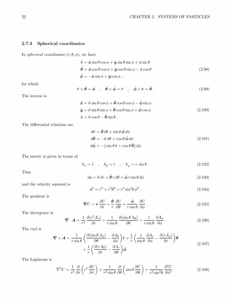
2.7.3 Spherical coordinates
In spherical coordinates (r, θ, φ), we have
r = x sin θ cosφ+ y sin θ sinφ+ z sin θ
θ = x cos θ cosφ+ y cos θ sinφ− z cos θφ = −x sinφ+ y cosφ ,
(2.98)
for whichr × θ = φ , θ × φ = r , φ× r = θ . (2.99)
The inverse is
x = r sin θ cosφ+ θ cos θ cosφ− φ sinφ
y = r sin θ sinφ+ θ cos θ sinφ+ φ cosφ
z = r cos θ − θ sin θ .(2.100)
The differential relations are
dr = θ dθ + sin θ φ dφ
dθ = −r dθ + cos θ φ dφ
dφ = −(sin θ r + cos θ θ
)dφ
(2.101)
The metric is given in terms of
hr = 1 , hθ = r , hφ = r sin θ . (2.102)
Thusds = r dr + θ r dθ + φ r sin θ dφ (2.103)
and the velocity squared iss2 = r2 + r2θ2 + r2 sin2θ φ2 . (2.104)
The gradient is
∇U = r∂U
∂r+θ
r
∂U
∂θ+
φ
r sin θ
∂U
∂φ. (2.105)
The divergence is
∇ ·A =1
r2∂(r2Ar)
∂r+
1
r sin θ
∂(sin θ Aθ)
∂θ+
1
r sin θ
∂Aφ
∂φ. (2.106)
The curl is
∇×A =1
r sin θ
(∂(sin θ Aφ)
∂θ− ∂Aθ
∂φ
)r +
1
r
(1
sin θ
∂Ar
∂φ− ∂(rAφ)
∂r
)θ
+1
r
(∂(rAθ)
∂r− ∂Ar
∂θ
)φ .
(2.107)
The Laplacian is
∇2U =1
r2∂
∂r
(r2∂U
∂r
)+
1
r2 sin θ
∂
∂θ
(sin θ
∂U
∂θ
)+
1
r2 sin2θ
∂2U
∂φ2. (2.108)

2.7. COMMON CURVILINEAR ORTHOGONAL SYSTEMS 23
2.7.4 Kinetic energy
Note the form of the kinetic energy of a point particle:
T = 12m
(ds
dt
)2= 1
2m(x2 + y2 + z2
)(3D Cartesian)
= 12m(ρ2 + ρ2φ2
)(2D polar)
= 12m(ρ2 + ρ2φ2 + z2
)(3D cylindrical)
= 12m(r2 + r2θ2 + r2 sin2θ φ2
)(3D polar) .
(2.109)

24 CHAPTER 2. SYSTEMS OF PARTICLES

Chapter 3
One-Dimensional Conservative Systems
3.1 Description as a Dynamical System
For one-dimensional mechanical systems, Newton’s second law reads
mx = F (x) . (3.1)
A system is conservative if the force is derivable from a potential: F = −dU/dx. The total energy,
E = T + U = 12mx
2 + U(x) , (3.2)
is then conserved. This may be verified explicitly:
dE
dt=
d
dt
[12mx
2 + U(x)]
=[mx+ U ′(x)
]x = 0 .
Conservation of energy allows us to reduce the equation of motion from second order to first order:
dx
dt= ±
√√√√ 2
m
(E − U(x)
). (3.3)
Note that the constant E is a constant of integration. The ± sign above depends on the direction ofmotion. Points x(E) which satisfy
E = U(x) ⇒ x(E) = U−1(E) , (3.4)
where U−1 is the inverse function, are called turning points. When the total energy is E, the motion ofthe system is bounded by the turning points, and confined to the region(s) U(x) ≤ E. We can integrateeqn. 3.3 to obtain
t(x)− t(x0) = ±√m
2
x∫
x0
dx′√E − U(x′)
. (3.5)
25

26 CHAPTER 3. ONE-DIMENSIONAL CONSERVATIVE SYSTEMS
This is to be inverted to obtain the function x(t). Note that there are now two constants of integration,
E and x0. Since
E = E0 =12mv
20 + U(x0) , (3.6)
we could also consider x0 and v0 as our constants of integration, writing E in terms of x0 and v0. Thus,there are two independent constants of integration.
For motion confined between two turning points x±(E), the period of the motion is given by
T (E) =√2m
x+(E)∫
x−(E)
dx′√E − U(x′)
. (3.7)
3.1.1 Example : harmonic oscillator
In the case of the harmonic oscillator, we have U(x) = 12kx
2, hence
dt
dx= ±
√m
2E − kx2. (3.8)
The turning points are x±(E) = ±√2E/k, for E ≥ 0. To solve for the motion, let us substitute
x =
√2E
ksin θ . (3.9)
We then find
dt =
√m
kdθ , (3.10)
with solutionθ(t) = θ0 + ωt , (3.11)
where ω =√k/m is the harmonic oscillator frequency. Thus, the complete motion of the system is given
by
x(t) =
√2E
ksin(ωt+ θ0) . (3.12)
Note the two constants of integration, E and θ0.
3.2 One-Dimensional Mechanics as a Dynamical System
Rather than writing the equation of motion as a single second order ODE, we can instead write it as twocoupled first order ODEs, viz.
dx
dt= v
dv
dt=
1
mF (x) .
(3.13)

3.2. ONE-DIMENSIONAL MECHANICS AS A DYNAMICAL SYSTEM 27
This may be written in matrix-vector form, as
d
dt
(xv
)=
(v
1m F (x)
). (3.14)
This is an example of a dynamical system, described by the general form
dϕ
dt= V (ϕ) , (3.15)
where ϕ = (ϕ1, . . . , ϕN ) is an N -dimensional vector in phase space. For the model of eqn. 3.14, weevidently have N = 2. The object V (ϕ) is called a vector field . It is itself a vector, existing at everypoint in phase space, RN . Each of the components of V (ϕ) is a function (in general) of all the componentsof ϕ:
Vj = Vj(ϕ1, . . . , ϕN ) (j = 1, . . . , N) . (3.16)
Solutions to the equation ϕ = V (ϕ) are called integral curves. Each such integral curve ϕ(t) is uniquelydetermined by N constants of integration, which may be taken to be the initial value ϕ(0). The collectionof all integral curves is known as the phase portrait of the dynamical system.
In plotting the phase portrait of a dynamical system, we need to first solve for its motion, starting fromarbitrary initial conditions. In general this is a difficult problem, which can only be treated numerically.But for conservative mechanical systems in d = 1, it is a trivial matter! The reason is that energyconservation completely determines the phase portraits. The velocity becomes a unique double-valued
function of position, v(x) = ±√
2m
(E − U(x)
). The phase curves are thus curves of constant energy.
3.2.1 Sketching phase curves
To plot the phase curves,
(i) Sketch the potential U(x).
(ii) Below this plot, sketch v(x;E) = ±√
2m
(E − U(x)
).
(iii) When E lies at a local extremum of U(x), the system is at a fixed point .
(a) For E slightly above Emin, the phase curves are ellipses.
(b) For E slightly below Emax, the phase curves are (locally) hyperbolae.
(c) For E = Emax the phase curve is called a separatrix .
(iv) When E > U(∞) or E > U(−∞), the motion is unbounded .
(v) Draw arrows along the phase curves: to the right for v > 0 and left for v < 0.
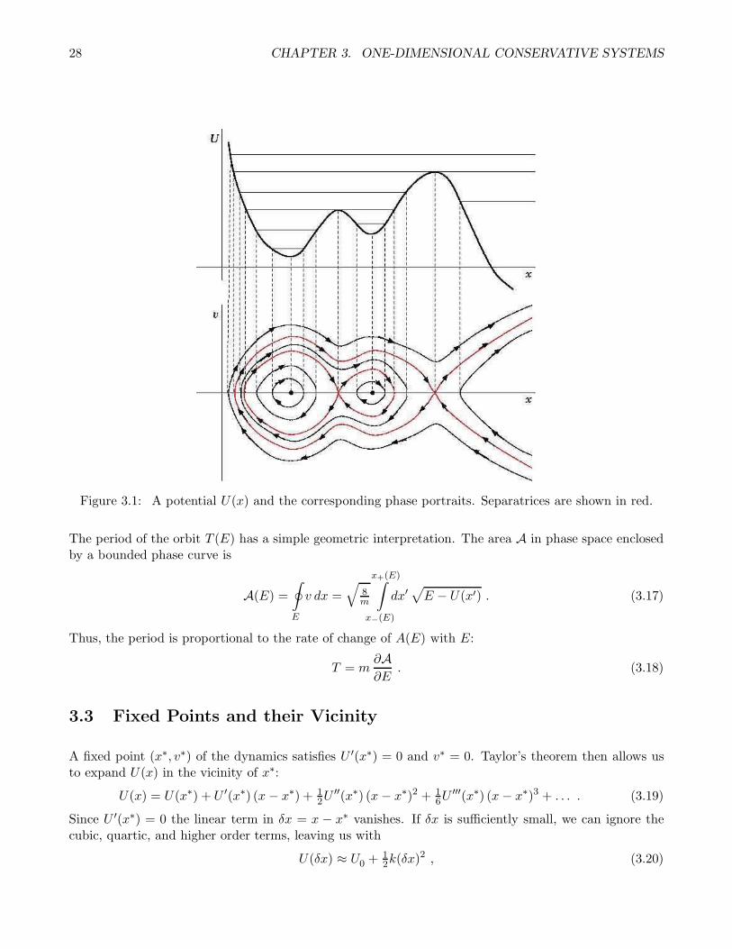
28 CHAPTER 3. ONE-DIMENSIONAL CONSERVATIVE SYSTEMS
Figure 3.1: A potential U(x) and the corresponding phase portraits. Separatrices are shown in red.
The period of the orbit T (E) has a simple geometric interpretation. The area A in phase space enclosedby a bounded phase curve is
A(E) =
∮
E
v dx =√
8m
x+(E)∫
x−(E)
dx′√E − U(x′) . (3.17)
Thus, the period is proportional to the rate of change of A(E) with E:
T = m∂A∂E
. (3.18)
3.3 Fixed Points and their Vicinity
A fixed point (x∗, v∗) of the dynamics satisfies U ′(x∗) = 0 and v∗ = 0. Taylor’s theorem then allows usto expand U(x) in the vicinity of x∗:
U(x) = U(x∗) + U ′(x∗) (x− x∗) + 12U
′′(x∗) (x− x∗)2 + 16U
′′′(x∗) (x− x∗)3 + . . . . (3.19)
Since U ′(x∗) = 0 the linear term in δx = x − x∗ vanishes. If δx is sufficiently small, we can ignore thecubic, quartic, and higher order terms, leaving us with
U(δx) ≈ U0 +12k(δx)
2 , (3.20)
3.3. FIXED POINTS AND THEIR VICINITY 29
where U0 = U(x∗) and k = U ′′(x∗) > 0. The solutions to the motion in this potential are:
U ′′(x∗) > 0 : δx(t) = δx0 cos(ωt) +δv0ω
sin(ωt)
U ′′(x∗) < 0 : δx(t) = δx0 cosh(γt) +δv0γ
sinh(γt) ,
(3.21)
where ω =√k/m for k > 0 and γ =
√−k/m for k < 0. The energy is
E = U0 +12m (δv0)
2 + 12k (δx0)
2 . (3.22)
For a separatrix, we have E = U0 and U ′′(x∗) < 0. From the equation for the energy, we obtain
δv0 = ±γ δx0. Let’s take δv0 = −γ δx0, so that the initial velocity is directed toward the unstable fixed
point (UFP). I.e. the initial velocity is negative if we are to the right of the UFP (δx0 > 0) and positive
if we are to the left of the UFP (δx0 < 0). The motion of the system is then
δx(t) = δx0 exp(−γt) . (3.23)
The particle gets closer and closer to the unstable fixed point at δx = 0, but it takes an infinite amount oftime to actually get there. Put another way, the time it takes to get from δx0 to a closer point δx < δx0is
t = γ−1 ln
(δx0δx
). (3.24)
This diverges logarithmically as δx → 0. Generically, then, the period of motion along a separatrix is
infinite.
3.3.1 Linearized dynamics in the vicinity of a fixed point
Linearizing in the vicinity of such a fixed point, we write δx = x− x∗ and δv = v − v∗, obtaining
d
dt
(δxδv
)=
(0 1
− 1m U ′′(x∗) 0
)(δxδv
)+ . . . , (3.25)
This is a linear equation, which we can solve completely.
Consider the general linear equation ϕ = Aϕ, where A is a fixed real matrix. Now whenever we havea problem involving matrices, we should start thinking about eigenvalues and eigenvectors. Invariably,the eigenvalues and eigenvectors will prove to be useful, if not essential, in solving the problem. Theeigenvalue equation is
Aψα = λαψα . (3.26)
Here ψα is the αth right eigenvector1 of A. The eigenvalues are roots of the characteristic equationP (λ) = 0, where P (λ) = det(λ · I−A). Let’s expand ϕ(t) in terms of the right eigenvectors of A:
ϕ(t) =∑
α
Cα(t)ψα . (3.27)
1If A is symmetric, the right and left eigenvectors are the same. If A is not symmetric, the right and left eigenvectors differ,although the set of corresponding eigenvalues is the same.

30 CHAPTER 3. ONE-DIMENSIONAL CONSERVATIVE SYSTEMS
Figure 3.2: Phase curves in the vicinity of centers and saddles.
Assuming, for the purposes of this discussion, that A is nondegenerate, and its eigenvectors span RN , thedynamical system can be written as a set of decoupled first order ODEs for the coefficients Cα(t):
Cα = λα Cα , (3.28)
with solutions
Cα(t) = Cα(0) exp(λαt) . (3.29)
If Re (λα) > 0, Cα(t) flows off to infinity, while if Re (λα) > 0, Cα(t) flows to zero. If |λα| = 1, then Cα(t)
oscillates with frequency Im (λα).
For a two-dimensional matrix, it is easy to show – an exercise for the reader – that
P (λ) = λ2 − Tλ+D , (3.30)
where T = Tr(A) and D = det(A). The eigenvalues are then
λ± = 12T ± 1
2
√T 2 − 4D . (3.31)
We’ll study the general case in Physics 110B. For now, we focus on our conservative mechanical systemof eqn. 3.25. The trace and determinant of the above matrix are T = 0 and D = 1
m U ′′(x∗). Thus, thereare only two (generic) possibilities: centers, when U ′′(x∗) > 0, and saddles, when U ′′(x∗) < 0. Examplesof each are shown in Fig. 3.1.

3.4. EXAMPLES OF CONSERVATIVE ONE-DIMENSIONAL SYSTEMS 31
Figure 3.3: Phase curves for the harmonic oscillator.
3.4 Examples of Conservative One-Dimensional Systems
3.4.1 Harmonic oscillator
Recall the harmonic oscillator. The potential energy is U(x) = 12kx
2. The equation of motion is
md2x
dt2= −dU
dx= −kx , (3.32)
where m is the mass and k the force constant (of a spring). With v = x, this may be written as theN = 2 system,
d
dt
(xv
)=
(0 1
−ω2 0
)(xv
)=
(v
−ω2 x
), (3.33)
where ω =√k/m has the dimensions of frequency (inverse time). The solution is well known:
x(t) = x0 cos(ωt) +v0ω
sin(ωt)
v(t) = v0 cos(ωt)− ω x0 sin(ωt) .(3.34)
The phase curves are ellipses:
ω0 x2(t) + ω−1
0 v2(t) = C , (3.35)
where C is a constant, independent of time. A sketch of the phase curves and of the phase flow is shownin Fig. 3.3. Note that the x and v axes have different dimensions.
Energy is conserved:
E = 12mv
2 + 12kx
2 . (3.36)
Therefore we may find the length of the semimajor and semiminor axes by setting v = 0 or x = 0, whichgives
xmax =
√2E
k, vmax =
√2E
m. (3.37)

32 CHAPTER 3. ONE-DIMENSIONAL CONSERVATIVE SYSTEMS
The area of the elliptical phase curves is thus
A(E) = π xmax vmax =2πE√mk
. (3.38)
The period of motion is therefore
T (E) = m∂A∂E
= 2π
√m
k, (3.39)
which is independent of E.
3.4.2 Pendulum
Next, consider the simple pendulum, composed of a mass point m affixed to a massless rigid rod of lengthℓ. The potential is U(θ) = −mgℓ cos θ, hence
mℓ2 θ = −dUdθ
= −mgℓ sin θ . (3.40)
This is equivalent tod
dt
(θω
)=
(ω
−ω20 sin θ
), (3.41)
where ω = θ is the angular velocity, and where ω0 =√g/ℓ is the natural frequency of small oscillations.
The conserved energy isE = 1
2 mℓ2 θ2 + U(θ) . (3.42)
Assuming the pendulum is released from rest at θ = θ0,
2E
mℓ2= θ2 − 2ω2
0 cos θ = −2ω20 cos θ0 . (3.43)
The period for motion of amplitude θ0 is then
T(θ0)=
√8
ω0
θ0∫
0
dθ√cos θ − cos θ0
=4
ω0K(sin2 1
2θ0), (3.44)
where K(z) is the complete elliptic integral of the first kind. Expanding K(z), we have
T(θ0)=
2π
ω0
1 + 1
4 sin2(12θ0)+ 9
64 sin4(12θ0)+ . . .
. (3.45)
For θ0 → 0, the period approaches the usual result 2π/ω0, valid for the linearized equation θ = −ω20 θ.
As θ0 → π2 , the period diverges logarithmically.
The phase curves for the pendulum are shown in Fig. 3.4. The small oscillations of the pendulum areessentially the same as those of a harmonic oscillator. Indeed, within the small angle approximation,sin θ ≈ θ, and the pendulum equations of motion are exactly those of the harmonic oscillator. These

3.4. EXAMPLES OF CONSERVATIVE ONE-DIMENSIONAL SYSTEMS 33
Figure 3.4: Phase curves for the simple pendulum. The separatrix divides phase space into regions ofrotation and libration.
oscillations are called librations. They involve a back-and-forth motion in real space, and the phase spacemotion is contractable to a point, in the topological sense. However, if the initial angular velocity islarge enough, a qualitatively different kind of motion is observed, whose phase curves are rotations. Inthis case, the pendulum bob keeps swinging around in the same direction, because, as we’ll see in a laterlecture, the total energy is sufficiently large. The phase curve which separates these two topologicallydistinct motions is called a separatrix .
3.4.3 Other potentials
Using the phase plotter application written by Ben Schmidel, available on the Physics 110A course webpage, it is possible to explore the phase curves for a wide variety of potentials. Three examples are shownin the following pages. The first is the effective potential for the Kepler problem,
Ueff(r) = −kr+
ℓ2
2µr2, (3.46)
about which we shall have much more to say when we study central forces. Here r is the separationbetween two gravitating bodies of masses m1,2, µ = m1m2/(m1 + m2) is the ‘reduced mass’, and k =
Gm1m2, where G is the Cavendish constant. We can then write
Ueff(r) = U0
− 1
x+
1
2x2
, (3.47)

34 CHAPTER 3. ONE-DIMENSIONAL CONSERVATIVE SYSTEMS
where r0 = ℓ2/µk has the dimensions of length, and x ≡ r/r0, and where U0 = k/r0 = µk2/ℓ2. Thus, if
distances are measured in units of r0 and the potential in units of U0, the potential may be written indimensionless form as U(x) = − 1
x + 12x2 .
The second is the hyperbolic secant potential,
U(x) = −U0 sech2(x/a) , (3.48)
which, in dimensionless form, is U(x) = −sech2(x), after measuring distances in units of a and potential
in units of U0.
The final example is
U(x) = U0
cos(xa
)+
x
2a
. (3.49)
Again measuring x in units of a and U in units of U0, we arrive at U(x) = cos(x) + 12x.

3.4. EXAMPLES OF CONSERVATIVE ONE-DIMENSIONAL SYSTEMS 35
Figure 3.5: Phase curves for the Kepler effective potential U(x) = −x−1 + 12x
−2.

36 CHAPTER 3. ONE-DIMENSIONAL CONSERVATIVE SYSTEMS
Figure 3.6: Phase curves for the potential U(x) = −sech2(x).

3.4. EXAMPLES OF CONSERVATIVE ONE-DIMENSIONAL SYSTEMS 37
Figure 3.7: Phase curves for the potential U(x) = cos(x) + 12x.

38 CHAPTER 3. ONE-DIMENSIONAL CONSERVATIVE SYSTEMS

Chapter 4
Linear Oscillations
Harmonic motion is ubiquitous in Physics. The reason is that any potential energy function, whenexpanded in a Taylor series in the vicinity of a local minimum, is a harmonic function:
U(~q ) = U(~q ∗) +N∑
j=1
∇U(~q∗)=0︷ ︸︸ ︷∂U
∂qj
∣∣∣∣~q=~q ∗
(qj − q∗j ) +12
N∑
j,k=1
∂2U
∂qj ∂qk
∣∣∣∣~q=~q ∗
(qj − q∗j ) (qk − q∗k) + . . . , (4.1)
where the qj are generalized coordinates – more on this when we discuss Lagrangians. In one dimension,we have simply
U(x) = U(x∗) + 12 U
′′(x∗) (x− x∗)2 + . . . . (4.2)
Provided the deviation η = x − x∗ is small enough in magnitude, the remaining terms in the Taylorexpansion may be ignored. Newton’s Second Law then gives
mη = −U ′′(x∗) η +O(η2) . (4.3)
This, to lowest order, is the equation of motion for a harmonic oscillator. If U ′′(x∗) > 0, the equilibriumpoint x = x∗ is stable, since for small deviations from equilibrium the restoring force pushes the systemback toward the equilibrium point. When U ′′(x∗) < 0, the equilibrium is unstable, and the forces pushone further away from equilibrium.
4.1 Damped Harmonic Oscillator
In the real world, there are frictional forces, which we here will approximate by F = −γv. We begin withthe homogeneous equation for a damped harmonic oscillator,
d2x
dt2+ 2β
dx
dt+ ω2
0 x = 0 , (4.4)
where γ = 2βm. To solve, write x(t) =∑
n Cn e−iωnt. This renders the differential equation 4.4 an
algebraic equation for the two eigenfrequencies ωi, each of which must satisfy
ω2 + 2iβω − ω20 = 0 , (4.5)
39

40 CHAPTER 4. LINEAR OSCILLATIONS
henceω± = −iβ ± (ω2
0 − β2)1/2 . (4.6)
The most general solution to eqn. 4.4 is then
x(t) = C+ e−iω+t + C− e
−iω−t (4.7)
where C± are arbitrary constants. Notice that the eigenfrequencies are in general complex, with a negative
imaginary part (so long as the damping coefficient β is positive). Thus e−iω±t decays to zero as t→ ∞.
4.1.1 Classes of damped harmonic motion
We identify three classes of motion:
(i) Underdamped (ω20 > β2)
(ii) Overdamped (ω20 < β2)
(iii) Critically Damped (ω20 = β2) .
Underdamped motion
The solution for underdamped motion is
x(t) = A cos(νt+ φ) e−βt
x(t) = −ω0A cos(νt+ φ+ sin−1(β/ω0)
)e−βt ,
(4.8)
where ν =√ω20 − β2, and where A and φ are constants determined by initial conditions. From x0 =
A cosφ and x0 = −βA cosφ− νA sinφ, we have x0 + βx0 = −νA sinφ, and
A =
√
x20 +
(x0 + β x0
ν
)2, φ = − tan−1
(x0 + β x0ν x0
). (4.9)
Overdamped motion
The solution in the case of overdamped motion is
x(t) = C e−(β−λ)t +D e−(β+λ)t
x(t) = −(β − λ)C e−(β−λ)t − (β + λ)D e−(β+λ)t ,(4.10)
where λ =√β2 − ω2
0 and where C and D are constants determined by the initial conditions:(
1 1−(β − λ) −(β + λ)
)(CD
)=
(x0x0
). (4.11)
Inverting the above matrix, we have the solution
C =(β + λ)x0
2λ+x02λ
, D = −(β − λ)x02λ
− x02λ
. (4.12)

4.1. DAMPED HARMONIC OSCILLATOR 41
Figure 4.1: Three classifications of damped harmonic motion. The initial conditions are x(0) = 1,x(0) = 0.
Critically damped motion
The solution in the case of critically damped motion is
x(t) = E e−βt + Ft e−βt
x(t) = −(βE + (βt− 1)F
)e−βt .
(4.13)
Thus, x0 = E and x0 = F − βE, so
E = x0 , F = x0 + βx0 . (4.14)
The screen door analogy
The three types of behavior are depicted in fig. 4.1. To concretize these cases in one’s mind, it is helpfulto think of the case of a screen door or a shock absorber. If the hinges on the door are underdamped,

42 CHAPTER 4. LINEAR OSCILLATIONS
the door will swing back and forth (assuming it doesn’t have a rim which smacks into the door frame)several times before coming to a stop. If the hinges are overdamped, the door may take a very long timeto close. To see this, note that for β ≫ ω0 we have
√β2 − ω2
0 = β
(1− ω2
0
β2
)−1/2
= β
(1− ω2
0
2β2− ω4
0
8β4+ . . .
),
(4.15)
which leads to
β −√β2 − ω2
0 =ω20
2β+
ω40
8β3+ . . .
β +√β2 − ω2
0 = 2β − ω20
2β−+ . . . .
(4.16)
Thus, we can write
x(t) = C e−t/τ1 +D e−t/τ2 , (4.17)
with
τ1 =1
β −√β2 − ω2
0
≈ 2β
ω20
τ2 =1
β +√β2 − ω2
0
≈ 1
2β.
(4.18)
Thus x(t) is a sum of exponentials, with decay times τ1,2. For β ≫ ω0, we have that τ1 is much larger
than τ2 – the ratio is τ1/τ2 ≈ 4β2/ω20 ≫ 1. Thus, on time scales on the order of τ1, the second term
has completely damped away. The decay time τ1, though, is very long, since β is so large. So a highlyoverdamped oscillator will take a very long time to come to equilbrium.
4.1.2 Remarks on the case of critical damping
Define the first order differential operator
Dt =d
dt+ β . (4.19)
The solution to Dt x(t) = 0 is x(t) = Ae−βt, where A is a constant. Note that the commutator of Dt andt is unity: [
Dt , t]= 1 , (4.20)
where [A,B] ≡ AB−BA. The simplest way to verify eqn. 4.20 is to compute its action upon an arbitraryfunction f(t):
[Dt , t
]f(t) =
(d
dt+ β
)t f(t)− t
(d
dt+ β
)f(t)
=d
dt
(t f(t)
)− t
d
dtf(t) = f(t) . (4.21)

4.1. DAMPED HARMONIC OSCILLATOR 43
Figure 4.2: Phase curves for the damped harmonic oscillator. Left panel: underdamped motion. Rightpanel: overdamped motion. Note the nullclines along v = 0 and v = −(ω2
0/2β)x, which are shown asdashed lines.
We know that x(t) = x(t) = Ae−βt satisfies Dt x(t) = 0. Therefore
0 = Dt
[Dt , t
]x(t)
= D2t
(t x(t)
)−Dt t
0︷ ︸︸ ︷Dt x(t)
= D2t
(t x(t)
).
(4.22)
We already know that D2t x(t) = DtDt x(t) = 0. The above equation establishes that the second inde-
pendent solution to the second order ODE D2t x(t) = 0 is x(t) = t x(t). Indeed, we can keep going, and
show that
Dnt
(tn−1 x(t)
)= 0 . (4.23)
Thus, the n independent solutions to the nth order ODE
(d
dt+ β
)nx(t) = 0 (4.24)
are
xk(t) = Atk e−βt , k = 0, 1, . . . , n − 1 . (4.25)

44 CHAPTER 4. LINEAR OSCILLATIONS
4.1.3 Phase portraits for the damped harmonic oscillator
Expressed as a dynamical system, the equation of motion x+ 2βx + ω20x = 0 is written as two coupled
first order ODEs, viz.
x = v
v = −ω20 x− 2βv .
(4.26)
In the theory of dynamical systems, a nullcline is a curve along which one component of the phase spacevelocity ϕ vanishes. In our case, there are two nullclines: x = 0 and v = 0. The equation of the firstnullcline, x = 0, is simply v = 0, i.e. the first nullcline is the x-axis. The equation of the second nullcline,v = 0, is v = −(ω2
0/2β)x. This is a line which runs through the origin and has negative slope. Everywherealong the first nullcline x = 0, we have that ϕ lies parallel to the v-axis. Similarly, everywhere along thesecond nullcline v = 0, we have that ϕ lies parallel to the x-axis. The situation is depicted in fig. 4.2.
4.2 Damped Harmonic Oscillator with Forcing
When forced, the equation for the damped oscillator becomes
d2x
dt2+ 2β
dx
dt+ ω2
0 x = f(t) , (4.27)
where f(t) = F (t)/m. Since this equation is linear in x(t), we can, without loss of generality, restrict outattention to harmonic forcing terms of the form
f(t) = f0 cos(Ωt+ ϕ0) = Re[f0 e
−iϕ0 e−iΩt]
(4.28)
where Re stands for “real part”. Here, Ω is the forcing frequency.
Consider first the complex equation
d2z
dt2+ 2β
dz
dt+ ω2
0 z = f0 e−iϕ0 e−iΩt . (4.29)
We try a solution z(t) = z0 e−iΩt. Plugging in, we obtain the algebraic equation
z0 =f0 e
−iϕ0
ω20 − 2iβΩ −Ω2
≡ A(Ω) eiδ(Ω) f0e−iϕ0 . (4.30)
The amplitude A(Ω) and phase shift δ(Ω) are given by the equation
A(Ω) eiδ(Ω) =1
ω20 − 2iβΩ −Ω2
. (4.31)
A basic fact of complex numbers:
1
a− ib=
a+ ib
a2 + b2=ei tan
−1(b/a)
√a2 + b2
. (4.32)

4.2. DAMPED HARMONIC OSCILLATOR WITH FORCING 45
Thus,
A(Ω) =((ω2
0 −Ω2)2 + 4β2Ω2)−1/2
δ(Ω) = tan−1
(2βΩ
ω20 −Ω2
).
(4.33)
Now since the coefficients β and ω20 are real, we can take the complex conjugate of eqn. 4.29, and write
z + 2β z + ω20 z = f0 e
−iϕ0 e−iΩt
¨z + 2β ˙z + ω20 z = f0 e
+iϕ0 e+iΩt ,(4.34)
where z is the complex conjugate of z. We now add these two equations and divide by two to arrive at
x+ 2β x+ ω20 x = f0 cos(Ωt+ ϕ0) . (4.35)
Therefore, the real, physical solution we seek is
xinh(t) = Re[A(Ω) eiδ(Ω) · f0 e−iϕ0 e−iΩt
]
= A(Ω) f0 cos(Ωt+ ϕ0 − δ(Ω)
).
(4.36)
The quantity A(Ω) is the amplitude of the response (in units of f0), while δ(Ω) is the (dimensionless)phase lag (typically expressed in radians).
The maximum of the amplitude A(Ω) occurs when A′(Ω) = 0. From
dA
dΩ= − 2Ω
[A(Ω)
]3(Ω2 − ω2
0 + 2β2), (4.37)
we conclude that A′(Ω) = 0 for Ω = 0 and for Ω = ΩR, where
ΩR =√ω20 − 2β2 . (4.38)
The solution at Ω = ΩR pertains only if ω20 > 2β2, of course, in which case Ω = 0 is a local minimum
and Ω = ΩR a local maximum. If ω20 < 2β2 there is only a local maximum, at Ω = 0. See Fig. 4.3.
Since equation 4.27 is linear, we can add a solution to the homogeneous equation to xinh(t) and we willstill have a solution. Thus, the most general solution to eqn. 4.27 is
x(t) = xinh(t) + xhom(t)
= Re[A(Ω) eiδ(Ω) · f0 e−iϕ0 e−iΩt
]+ C+ e
−iω+t + C− e−iω
−t
=
xinh(t)︷ ︸︸ ︷A(Ω) f0 cos
(Ωt+ ϕ0 − δ(Ω)
)+
xhom(t)︷ ︸︸ ︷C e−βt cos(νt) +D e−βt sin(νt) ,
(4.39)

46 CHAPTER 4. LINEAR OSCILLATIONS
Figure 4.3: Amplitude and phase shift versus oscillator frequency (units of ω0) for β/ω0 values of 0.1(red), 0.25 (magenta), 1.0 (green), and 2.0 (blue).
where ν =√ω20 − β2 as before.
The last two terms in eqn. 4.39 are the solution to the homogeneous equation, i.e. with f(t) = 0. Theyare necessary to include because they carry with them the two constants of integration which always arisein the solution of a second order ODE. That is, C and D are adjusted so as to satisfy x(0) = x0 and
x0 = v0. However, due to their e−βt prefactor, these terms decay to zero once t reaches a relatively lowmultiple of β−1. They are called transients, and may be set to zero if we are only interested in the longtime behavior of the system. This means, incidentally, that the initial conditions are effectively forgottenover a time scale on the order of β−1.
For ΩR > 0, one defines the quality factor , Q, of the oscillator by Q = ΩR/2β. Q is a rough measure ofhow many periods the unforced oscillator executes before its initial amplitude is damped down to a smallvalue. For a forced oscillator driven near resonance, and for weak damping, Q is also related to the ratioof average energy in the oscillator to the energy lost per cycle by the external source. To see this, let uscompute the energy lost per cycle,
∆E = m
2π/Ω∫
0
dt x f(t)
= −m2π/Ω∫
0
dtΩ Af20 sin(Ωt+ ϕ0 − δ) cos(Ωt+ ϕ0)
= πAf20 m sin δ = 2πβmΩA2(Ω) f20 ,
(4.40)

4.2. DAMPED HARMONIC OSCILLATOR WITH FORCING 47
since sin δ(Ω) = 2βΩ A(Ω). The oscillator energy, averaged over the cycle, is
⟨E⟩=Ω
2π
2π/Ω∫
0
dt 12m(x2 + ω2
0 x2)
= 14m (Ω2 + ω2
0)A2(Ω) f20 .
(4.41)
Thus, we have
2π〈E〉∆E
=Ω2 + ω2
0
4βΩ. (4.42)
Thus, for Ω ≈ ΩR and β2 ≪ ω20, we have
Q ≈ 2π〈E〉∆E
≈ ω0
2β. (4.43)
4.2.1 Resonant forcing
When the damping β vanishes, the response diverges at resonance. The solution to the resonantly forcedoscillator
x+ ω20 x = f0 cos(ω0 t+ ϕ0) (4.44)
is given by
x(t) =f02ω0
t sin(ω0 t+ ϕ0)+
xhom(t)︷ ︸︸ ︷A cos(ω0 t) +B sin(ω0 t) . (4.45)
The amplitude of this solution grows linearly due to the energy pumped into the oscillator by the resonantexternal forcing. In the real world, nonlinearities can mitigate this unphysical, unbounded response.
4.2.2 R-L-C circuits
Consider the R-L-C circuit of Fig. 4.4. When the switch is to the left, the capacitor is charged, eventuallyto a steady state value Q = CV . At t = 0 the switch is thrown to the right, completing the R-L-C circuit.Recall that the sum of the voltage drops across the three elements must be zero:
LdI
dt+ IR+
Q
C= 0 . (4.46)
We also have Q = I, hence
d2Q
dt2+R
L
dQ
dt+
1
LCQ = 0 , (4.47)
which is the equation for a damped harmonic oscillator, with ω0 = (LC)−1/2 and β = R/2L.

48 CHAPTER 4. LINEAR OSCILLATIONS
Figure 4.4: An R-L-C circuit which behaves as a damped harmonic oscillator.
The boundary conditions at t = 0 are Q(0) = CV and Q(0) = 0. Under these conditions, the full solutionat all times is
Q(t) = CV e−βt(cos νt+
β
νsin νt
)
I(t) = −CV ω20
νe−βt sin νt ,
(4.48)
again with ν =√ω20 − β2.
If we put a time-dependent voltage source in series with the resistor, capacitor, and inductor, we wouldhave
LdI
dt+ IR+
Q
C= V (t) , (4.49)
which is the equation of a forced damped harmonic oscillator.
4.2.3 Examples
Third order linear ODE with forcing
The problem is to solve the equation
Lt x ≡ ˙x+ (a+ b+ c) x+ (ab+ ac+ bc) x+ abc x = f0 cos(Ωt) . (4.50)
The key to solving this is to note that the differential operator Lt factorizes:
Lt =d3
dt3+ (a+ b+ c)
d2
dt2+ (ab+ ac+ bc)
d
dt+ abc
=( ddt
+ a)( d
dt+ b)( d
dt+ c),
(4.51)
which says that the third order differential operator appearing in the ODE is in fact a product of firstorder differential operators. Since
dx
dt+ αx = 0 =⇒ x(t) = Ae−αx , (4.52)

4.2. DAMPED HARMONIC OSCILLATOR WITH FORCING 49
Figure 4.5: A driven L-C-R circuit, with V (t) = V0 cos(ωt).
we see that the homogeneous solution takes the form
xh(t) = Ae−at +B e−bt + C e−ct , (4.53)
where A, B, and C are constants.
To find the inhomogeneous solution, we solve Lt x = f0 e−iΩt and take the real part. Writing x(t) =
x0 e−iΩt, we have
Lt x0 e−iΩt = (a− iΩ) (b− iΩ) (c − iΩ)x0 e
−iΩt (4.54)
and thus
x0 =f0 e
−iΩt
(a− iΩ)(b− iΩ)(c − iΩ)≡ A(Ω) eiδ(Ω) f0 e
−iΩt , (4.55)
where
A(Ω) =[(a2 +Ω2) (b2 +Ω2) (c2 +Ω2)
]−1/2
δ(Ω) = tan−1(Ωa
)+ tan−1
(Ωb
)+ tan−1
(Ωc
).
(4.56)
Thus, the most general solution to Lt x(t) = f0 cos(Ωt) is
x(t) = A(Ω) f0 cos(Ωt− δ(Ω)
)+Ae−at +B e−bt + C e−ct . (4.57)
Note that the phase shift increases monotonically from δ(0) = 0 to δ(∞) = 32π.
Mechanical analog of RLC circuit
Consider the electrical circuit in fig. 4.5. Our task is to construct its mechanical analog. To do so, weinvoke Kirchoff’s laws around the left and right loops:
L1 I1 +Q1
C1+R1 (I1 − I2) = 0
L2 I2 +R2 I2 +R1 (I2 − I1) = V (t) .
(4.58)

50 CHAPTER 4. LINEAR OSCILLATIONS
Figure 4.6: The equivalent mechanical circuit for fig. 4.5.
Let Q1(t) be the charge on the left plate of capacitor C1, and define
Q2(t) =
t∫
0
dt′ I2(t′) . (4.59)
Then Kirchoff’s laws may be written
Q1 +R1
L1(Q1 − Q2) +
1
L1C1Q1 = 0
Q2 +R2
L2Q2 +
R1
L2(Q2 − Q1) =
V (t)
L2.
(4.60)
Now consider the mechanical system in Fig. 4.6. The blocks have masses M1 and M2. The frictioncoefficient between blocks 1 and 2 is b1, and the friction coefficient between block 2 and the floor isb2. Here we assume a velocity-dependent frictional force Ff = −bx, rather than the more conventional
constant Ff = −µW , where W is the weight of an object. Velocity-dependent friction is applicable whenthe relative velocity of an object and a surface is sufficiently large. There is a spring of spring constantk1 which connects block 1 to the wall. Finally, block 2 is driven by a periodic acceleration f0 cos(ωt).We now identify
X1 ↔ Q1 , X2 ↔ Q2 , b1 ↔R1
L1, b2 ↔
R2
L2, k1 ↔
1
L1C1, (4.61)
as well as f(t) ↔ V (t)/L2.
The solution again proceeds by Fourier transform. We write
V (t) =
∞∫
−∞
dω
2πV (ω) e−iωt (4.62)
and Q1(t)
I2(t)
=
∞∫
−∞
dω
2π
Q1(ω)
I2(ω)
e−iωt (4.63)

4.3. GENERAL SOLUTION BY GREEN’S FUNCTION METHOD 51
The frequency space version of Kirchoff’s laws for this problem is
G(ω)︷ ︸︸ ︷−ω2 − iω R1/L1 + 1/L1 C1 R1/L1
iω R1/L2 −iω + (R1 +R2)/L2
Q1(ω)
I2(ω)
=
0
V (ω)/L2
(4.64)
The homogeneous equation has eigenfrequencies given by the solution to det G(ω) = 0, which is a cubic
equation. Correspondingly, there are three initial conditions to account for: Q1(0), I1(0), and I2(0). Asin the case of the single damped harmonic oscillator, these transients are damped, and for large timesmay be ignored. The solution then is
Q1(ω)
I2(ω)
=
−ω2 − iω R1/L1 + 1/L1 C1 R1/L1
iω R1/L2 −iω + (R1 +R2)/L2
−1
0
V (ω)/L2
. (4.65)
To obtain the time-dependent Q1(t) and I2(t), we must compute the Fourier transform back to the timedomain.
4.3 General solution by Green’s function method
For a general forcing function f(t), we solve by Fourier transform. Recall that a function F (t) in thetime domain has a Fourier transform F (ω) in the frequency domain. The relation between the two is:1
F (t) =
∞∫
−∞
dω
2πe−iωt F (ω) ⇐⇒ F (ω) =
∞∫
−∞
dt e+iωt F (t) . (4.66)
We can convert the differential equation 4.3 to an algebraic equation in the frequency domain, x(ω) =G(ω) f(ω), where
G(ω) =1
ω20 − 2iβω − ω2
(4.67)
is the Green’s function in the frequency domain. The general solution is written
x(t) =
∞∫
−∞
dω
2πe−iωt G(ω) f(ω) + xh(t) , (4.68)
1Different texts often use different conventions for Fourier and inverse Fourier transforms. Sometimes the factor of (2π)−1
is associated with the time integral, and sometimes a factor of (2π)−1/2 is assigned to both frequency and time integrals.The convention I use is obviously the best.

52 CHAPTER 4. LINEAR OSCILLATIONS
where xh(t) =∑
iCi e−iωit is a solution to the homogeneous equation. We may also write the above
integral over the time domain:
x(t) =
∞∫
−∞
dt′G(t− t′) f(t′) + xh(t)
G(s) =
∞∫
−∞
dω
2πe−iωs G(ω)
= ν−1 exp(−βs) sin(νs)Θ(s)
(4.69)
where Θ(s) is the step function,
Θ(s) =
1 if s ≥ 00 if s < 0
(4.70)
where once again ν ≡√ω20 − β2.
Example: force pulse
Consider a pulse force
f(t) = f0Θ(t)Θ(T − t) =
f0 if 0 ≤ t ≤ T0 otherwise.
(4.71)
In the underdamped regime, for example, we find the solution
x(t) =f0ω20
1− e−βt cos νt− β
νe−βt sin νt
(4.72)
if 0 ≤ t ≤ T and
x(t) =f0ω20
(e−β(t−T ) cos ν(t− T )− e−βt cos νt
)
+β
ν
(e−β(t−T ) sin ν(t− T )− e−βt sin νt
) (4.73)
if t > T .
4.4 General Linear Autonomous Inhomogeneous ODEs
This method immediately generalizes to the case of general autonomous linear inhomogeneous ODEs ofthe form
dnx
dtn+ an−1
dn−1x
dtn−1+ . . . + a1
dx
dt+ a0 x = f(t) . (4.74)
We can write this asLt x(t) = f(t) , (4.75)

4.4. GENERAL LINEAR AUTONOMOUS INHOMOGENEOUS ODES 53
Figure 4.7: Response of an underdamped oscillator to a pulse force.
where Lt is the nth order differential operator
Lt =dn
dtn+ an−1
dn−1
dtn−1+ . . .+ a1
d
dt+ a0 . (4.76)
The general solution to the inhomogeneous equation is given by
x(t) = xh(t) +
∞∫
−∞
dt′ G(t, t′) f(t′) , (4.77)
where G(t, t′) is the Green’s function. Note that Lt xh(t) = 0. Thus, in order for eqns. 4.75 and 4.77 tobe true, we must have
Lt x(t) =
this vanishes︷ ︸︸ ︷Lt xh(t) +
∞∫
−∞
dt′ LtG(t, t′) f(t′) = f(t) , (4.78)
which means that
LtG(t, t′) = δ(t− t′) , (4.79)

54 CHAPTER 4. LINEAR OSCILLATIONS
where δ(t− t′) is the Dirac δ-function. Some properties of δ(x):
b∫
a
dx f(x) δ(x − y) =
f(y) if a < y < b
0 if y < a or y > b .
(4.80)
δ(g(x)
)=
∑
xiwith
g(xi)=0
δ(x− xi)∣∣g′(xi)∣∣ , (4.81)
valid for any functions f(x) and g(x). The sum in the second equation is over the zeros xi of g(x).
Incidentally, the Dirac δ-function enters into the relation between a function and its Fourier transform,in the following sense. We have
f(t) =
∞∫
−∞
dω
2πe−iωt f(ω)
f(ω) =
∞∫
−∞
dt e+iωt f(t) .
(4.82)
Substituting the second equation into the first, we have
f(t) =
∞∫
−∞
dω
2πe−iωt
∞∫
−∞
dt′ eiωt′
f(t′)
=
∞∫
−∞
dt′ ∞∫
−∞
dω
2πeiω(t
′−t)
f(t′) ,
(4.83)
which is indeed correct because the term in brackets is a representation of δ(t − t′):
∞∫
−∞
dω
2πeiωs = δ(s) . (4.84)
If the differential equation Lt x(t) = f(t) is defined over some finite t interval with prescribed boundaryconditions on x(t) at the endpoints, then G(t, t′) will depend on t and t′ separately. For the case we areconsidering, the interval is the entire real line t ∈ (−∞,∞), and G(t, t′) = G(t − t′) is a function of thesingle variable t− t′.
Note that Lt = L(ddt
)may be considered a function of the differential operator d
dt . If we now Fourier

4.4. GENERAL LINEAR AUTONOMOUS INHOMOGENEOUS ODES 55
transform the equation Lt x(t) = f(t), we obtain
∞∫
−∞
dt eiωt f(t) =
∞∫
−∞
dt eiωtdn
dtn+ an−1
dn−1
dtn−1+ . . .+ a1
d
dt+ a0
x(t)
=
∞∫
−∞
dt eiωt
(−iω)n + an−1 (−iω)n−1 + . . .+ a1 (−iω) + a0
x(t) ,
(4.85)
where we integrate by parts on t, assuming the boundary terms at t = ±∞ vanish, i.e. x(±∞) = 0, sothat, inside the t integral,
eiωt(d
dt
)kx(t) →
[(− d
dt
)keiωt
]x(t) = (−iω)k eiωt x(t) . (4.86)
Thus, if we define
L(ω) =n∑
k=0
ak (−iω)k , (4.87)
then we have
L(ω) x(ω) = f(ω) , (4.88)
where an ≡ 1. According to the Fundamental Theorem of Algebra, the nth degree polynomial L(ω) maybe uniquely factored over the complex ω plane into a product over n roots:
L(ω) = (−i)n (ω − ω1)(ω − ω2) · · · (ω − ωn) . (4.89)
If the ak are all real, then[L(ω)
]∗= L(−ω∗), hence if Ω is a root then so is −Ω∗. Thus, the roots
appear in pairs which are symmetric about the imaginary axis. I.e. if Ω = a + ib is a root, then so is−Ω∗ = −a+ ib.
The general solution to the homogeneous equation is
xh(t) =
n∑
i=1
Ai e−iωit , (4.90)
which involves n arbitrary complex constants Ai. The susceptibility, or Green’s function in Fourier space,G(ω) is then
G(ω) =1
L(ω)=
in
(ω − ω1)(ω − ω2) · · · (ω − ωn), (4.91)
and the general solution to the inhomogeneous equation is again given by
x(t) = xh(t) +
∞∫
−∞
dt′ G(t− t′) f(t′) , (4.92)

56 CHAPTER 4. LINEAR OSCILLATIONS
where xh(t) is the solution to the homogeneous equation, i.e. with zero forcing, and where
G(s) =
∞∫
−∞
dω
2πe−iωs G(ω)
= in∞∫
−∞
dω
2π
e−iωs
(ω − ω1)(ω − ω2) · · · (ω − ωn)
=
n∑
j=1
e−iωjs
iL′(ωj)Θ(s) ,
(4.93)
where we assume that Imωj < 0 for all j. The integral above was done using Cauchy’s theorem and thecalculus of residues – a beautiful result from the theory of complex functions.
As an example, consider the familiar case
L(ω) = ω20 − 2iβω − ω2
= −(ω − ω+) (ω − ω−) ,(4.94)
with ω± = −iβ ± ν, and ν = (ω20 − β2)1/2. This yields
L′(ω±) = ∓(ω+ − ω−) = ∓2ν . (4.95)
Then according to equation 4.93,
G(s) =
e−iω+s
iL′(ω+)+
e−iω−s
iL′(ω−)
Θ(s)
=
e−βs e−iνs
−2iν+e−βs eiνs
2iν
Θ(s)
= ν−1 e−βs sin(νs)Θ(s) ,
(4.96)
exactly as before.
4.5 Kramers-Kronig Relations (advanced material)
Suppose χ(ω) ≡ G(ω) is analytic in the UHP2. Then for all ν, we must have
∞∫
−∞
dν
2π
χ(ν)
ν − ω + iǫ= 0 , (4.97)
2In this section, we use the notation χ(ω) for the susceptibility, rather than G(ω)

4.5. KRAMERS-KRONIG RELATIONS (ADVANCED MATERIAL) 57
where ǫ is a positive infinitesimal. The reason is simple: just close the contour in the UHP, assumingχ(ω) vanishes sufficiently rapidly that Jordan’s lemma can be applied. Clearly this is an extremely weakrestriction on χ(ω), given the fact that the denominator already causes the integrand to vanish as |ω|−1.
Let us examine the function
1
ν − ω + iǫ=
ν − ω
(ν − ω)2 + ǫ2− iǫ
(ν − ω)2 + ǫ2. (4.98)
which we have separated into real and imaginary parts. Under an integral sign, the first term, in thelimit ǫ→ 0, is equivalent to taking a principal part of the integral. That is, for any function F (ν) whichis regular at ν = ω,
limǫ→0
∞∫
−∞
dν
2π
ν − ω
(ν − ω)2 + ǫ2F (ν) ≡ P
∞∫
−∞
dν
2π
F (ν)
ν − ω. (4.99)
The principal part symbol P means that the singularity at ν = ω is elided, either by smoothing out thefunction 1/(ν − ǫ) as above, or by simply cutting out a region of integration of width ǫ on either side ofν = ω.
The imaginary part is more interesting. Let us write
h(u) ≡ ǫ
u2 + ǫ2. (4.100)
For |u| ≫ ǫ, h(u) ≃ ǫ/u2, which vanishes as ǫ→ 0. For u = 0, h(0) = 1/ǫ which diverges as ǫ→ 0. Thus,h(u) has a huge peak at u = 0 and rapidly decays to 0 as one moves off the peak in either direction adistance greater that ǫ. Finally, note that
∞∫
−∞
duh(u) = π , (4.101)
a result which itself is easy to show using contour integration. Putting it all together, this tells us that
limǫ→0
ǫ
u2 + ǫ2= πδ(u) . (4.102)
Thus, for positive infinitesimal ǫ,1
u± iǫ= P 1
u∓ iπδ(u) , (4.103)
a most useful result.
We now return to our initial result 4.97, and we separate χ(ω) into real and imaginary parts:
χ(ω) = χ′(ω) + iχ′′(ω) . (4.104)
(In this equation, the primes do not indicate differentiation with respect to argument.) We thereforehave, for every real value of ω,
0 =
∞∫
−∞
dν
2π
[χ′(ν) + iχ′′(ν)
] [P 1
ν − ω− iπδ(ν − ω)
]. (4.105)
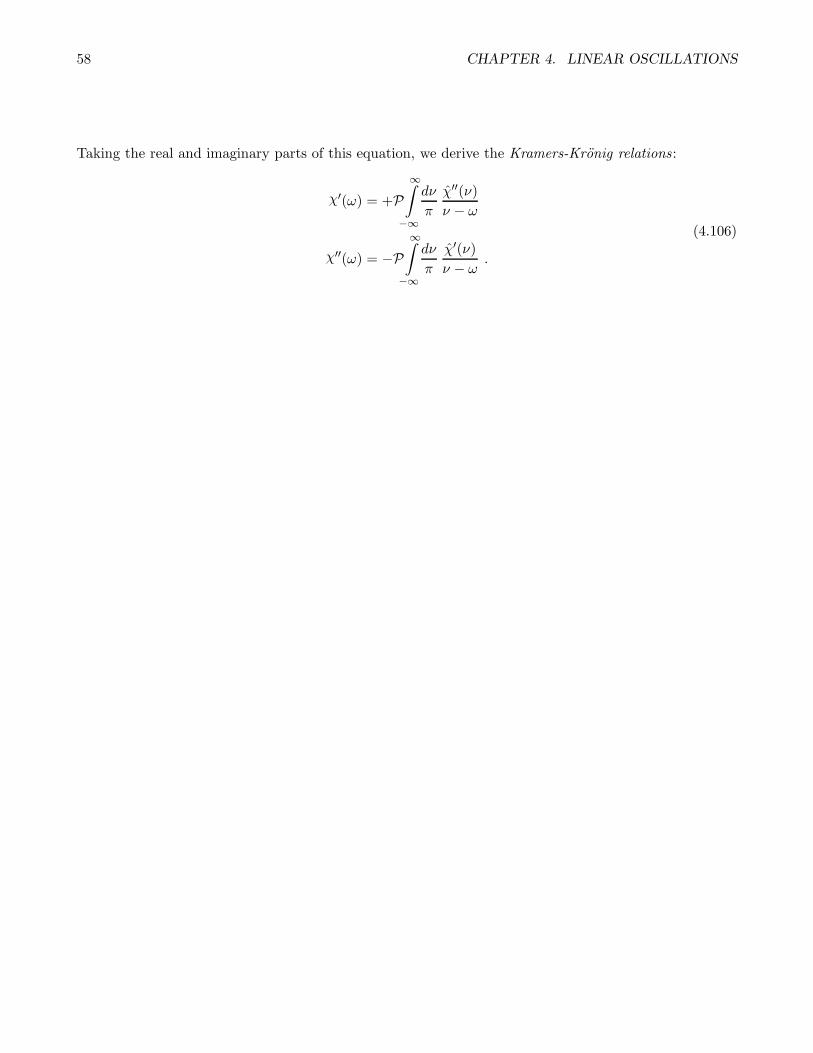
58 CHAPTER 4. LINEAR OSCILLATIONS
Taking the real and imaginary parts of this equation, we derive the Kramers-Kronig relations:
χ′(ω) = +P∞∫
−∞
dν
π
χ′′(ν)
ν − ω
χ′′(ω) = −P∞∫
−∞
dν
π
χ′(ν)
ν − ω.
(4.106)

Chapter 5
Calculus of Variations
5.1 Snell’s Law
Warm-up problem: You are standing at point (x1, y1) on the beach and you want to get to a point (x2, y2)in the water, a few meters offshore. The interface between the beach and the water lies at x = 0. Whatpath results in the shortest travel time? It is not a straight line! This is because your speed v1 on the
sand is greater than your speed v2 in the water. The optimal path actually consists of two line segments,as shown in Fig. 5.1. Let the path pass through the point (0, y) on the interface. Then the time T is afunction of y:
T (y) =1
v1
√x21 + (y − y1)
2 +1
v2
√x22 + (y2 − y)2 . (5.1)
To find the minimum time, we set
dT
dy= 0 =
1
v1
y − y1√x21 + (y − y1)
2
− 1
v2
y2 − y√x22 + (y2 − y)2
=sin θ1v1
− sin θ2v2
.
(5.2)
Thus, the optimal path satisfiessin θ1sin θ2
=v1v2
, (5.3)
which is known as Snell’s Law.
Snell’s Law is familiar from optics, where the speed of light in a polarizable medium is written v = c/n,where n is the index of refraction. In terms of n,
n1 sin θ1 = n2 sin θ2 . (5.4)
If there are several interfaces, Snell’s law holds at each one, so that
ni sin θi = ni+1 sin θi+1 , (5.5)
59
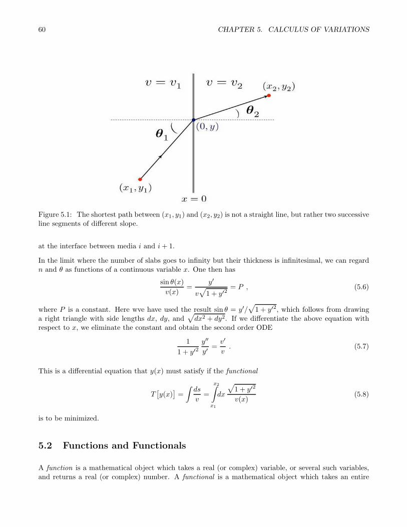
60 CHAPTER 5. CALCULUS OF VARIATIONS
Figure 5.1: The shortest path between (x1, y1) and (x2, y2) is not a straight line, but rather two successiveline segments of different slope.
at the interface between media i and i+ 1.
In the limit where the number of slabs goes to infinity but their thickness is infinitesimal, we can regardn and θ as functions of a continuous variable x. One then has
sin θ(x)
v(x)=
y′
v√
1 + y′2= P , (5.6)
where P is a constant. Here wve have used the result sin θ = y′/√
1 + y′2, which follows from drawinga right triangle with side lengths dx, dy, and
√dx2 + dy2. If we differentiate the above equation with
respect to x, we eliminate the constant and obtain the second order ODE
1
1 + y′2y′′
y′=v′
v. (5.7)
This is a differential equation that y(x) must satisfy if the functional
T[y(x)
]=
∫ds
v=
x2∫
x1
dx
√1 + y′2
v(x)(5.8)
is to be minimized.
5.2 Functions and Functionals
A function is a mathematical object which takes a real (or complex) variable, or several such variables,and returns a real (or complex) number. A functional is a mathematical object which takes an entire

5.2. FUNCTIONS AND FUNCTIONALS 61
Figure 5.2: The path of shortest length is composed of three line segments. The relation between theangles at each interface is governed by Snell’s Law.
function and returns a number. In the case at hand, we have
T[y(x)
]=
x2∫
x1
dxL(y, y′, x) , (5.9)
where the function L(y, y′, x) is given by
L(y, y′, x) =1
v(x)
√1 + y′2 . (5.10)
Here v(x) is a given function characterizing the medium, and y(x) is the path whose time is to beevaluated.
In ordinary calculus, we extremize a function f(x) by demanding that f not change to lowest order whenwe change x→ x+ dx:
f(x+ dx) = f(x) + f ′(x) dx+ 12 f
′′(x) (dx)2 + . . . . (5.11)
We say that x = x∗ is an extremum when f ′(x∗) = 0.
For a functional, the first functional variation is obtained by sending y(x) → y(x)+δy(x), and extracting

62 CHAPTER 5. CALCULUS OF VARIATIONS
Figure 5.3: A path y(x) and its variation y(x) + δy(x).
the variation in the functional to order δy. Thus, we compute
T[y(x) + δy(x)
]=
x2∫
x1
dxL(y + δy, y′ + δy′, x)
=
x2∫
x1
dx
L+
∂L
∂yδy +
∂L
∂y′δy′ +O
((δy)2
)
= T[y(x)
]+
x2∫
x1
dx
∂L
∂yδy +
∂L
∂y′d
dxδy
= T[y(x)
]+
x2∫
x1
dx
[∂L
∂y− d
dx
(∂L
∂y′
)]δy +
∂L
∂y′δy
∣∣∣∣∣
x2
x1
.
(5.12)
Now one very important thing about the variation δy(x) is that it must vanish at the endpoints: δy(x1) =
δy(x2) = 0. This is because the space of functions under consideration satisfy fixed boundary conditions
y(x1) = y1 and y(x2) = y2. Thus, the last term in the above equation vanishes, and we have
δT =
x2∫
x1
dx
[∂L
∂y− d
dx
(∂L
∂y′
)]δy . (5.13)
We say that the first functional derivative of T with respect to y(x) is
δT
δy(x)=
[∂L
∂y− d
dx
(∂L
∂y′
)]
x
, (5.14)
where the subscript indicates that the expression inside the square brackets is to be evaluated at x. Thefunctional T
[y(x)
]is extremized when its first functional derivative vanishes, which results in a differential

5.2. FUNCTIONS AND FUNCTIONALS 63
equation for y(x),
∂L
∂y− d
dx
(∂L
∂y′
)= 0 , (5.15)
known as the Euler-Lagrange equation.
L(y, y′, x) independent of y
Suppose L(y, y′, x) is independent of y. Then from the Euler-Lagrange equations we have that
P ≡ ∂L
∂y′(5.16)
is a constant. In classical mechanics, this will turn out to be a generalized momentum. For L = 1v
√1 + y′2,
we have
P =y′
v√
1 + y′2. (5.17)
Setting dP/dx = 0, we recover the second order ODE of eqn. 5.7. Solving for y′,
dy
dx= ± v(x)√
v20 − v2(x), (5.18)
where v0 = 1/P .
L(y, y′, x) independent of x
When L(y, y′, x) is independent of x, we can again integrate the equation of motion. Consider the quantity
H = y′∂L
∂y′− L . (5.19)
Then
dH
dx=
d
dx
[y′∂L
∂y′− L
]= y′′
∂L
∂y′+ y′
d
dx
(∂L
∂y′
)− ∂L
∂y′y′′ − ∂L
∂yy′ − ∂L
∂x
= y′[d
dx
(∂L
∂y′
)− ∂L
∂y
]− ∂L
∂x,
(5.20)
where we have used the Euler-Lagrange equations to write ddx
(∂L∂y′
)= ∂L
∂y . So if ∂L/∂x = 0, we havedH/dx = 0, i.e. H is a constant.
64 CHAPTER 5. CALCULUS OF VARIATIONS
5.2.1 Functional Taylor series
In general, we may expand a functional F [y + δy] in a functional Taylor series,
F [y + δy] = F [y] +
∫dx1K1(x1) δy(x1) +
12 !
∫dx1
∫dx2K2(x1, x2) δy(x1) δy(x2)
+ 13 !
∫dx1
∫dx2
∫dx3K3(x1, x2, x3) δy(x1) δy(x2) δy(x3) + . . .
(5.21)
and we write
Kn(x1, . . . , xn) ≡δnF
δy(x1) · · · δy(xn)(5.22)
for the nth functional derivative.
5.3 Examples from the Calculus of Variations
Here we present three useful examples of variational calculus as applied to problems in mathematics andphysics.
5.3.1 Example 1 : minimal surface of revolution
Consider a surface formed by rotating the function y(x) about the x-axis. The area is then
A[y(x)
]=
x2∫
x1
dx 2πy
√
1 +
(dy
dx
)2, (5.23)
and is a functional of the curve y(x). Thus we can define L(y, y′) = 2πy√
1 + y′2 and make the identifi-cation y(x) ↔ q(t). Since L(y, y′, x) is independent of x, we have
H = y′∂L
∂y′− L ⇒ dH
dx= −∂L
∂x, (5.24)
and when L has no explicit x-dependence, H is conserved. One finds
H = 2πy · y′2√1 + y′2
− 2πy
√1 + y′2 = − 2πy√
1 + y′2. (5.25)
Solving for y′,
dy
dx= ±
√(2πy
H
)2
− 1 , (5.26)
which may be integrated with the substitution y = H2π coshu, yielding
y(x) = b cosh
(x− a
b
), (5.27)

5.3. EXAMPLES FROM THE CALCULUS OF VARIATIONS 65
Figure 5.4: Minimal surface solution, with y(x) = b cosh(x/b) and y(x0) = y0. Top panel: A/2πy20 vs.
y0/x0. Bottom panel: sech(x0/b) vs. y0/x0. The blue curve corresponds to a global minimum of A[y(x)],and the red curve to a local minimum or saddle point.
where a and b = H2π are constants of integration. Note there are two such constants, as the original
equation was second order. This shape is called a catenary. As we shall later find, it is also the shape of auniformly dense rope hanging between two supports, under the influence of gravity. To fix the constantsa and b, we invoke the boundary conditions y(x1) = y1 and y(x2) = y2.
Consider the case where −x1 = x2 ≡ x0 and y1 = y2 ≡ y0. Then clearly a = 0, and we have
y0 = b cosh(x0b
)⇒ γ = κ−1 coshκ , (5.28)
with γ ≡ y0/x0 and κ ≡ x0/b. One finds that for any γ > 1.5089 there are two solutions, one of whichis a global minimum and one of which is a local minimum or saddle of A[y(x)]. The solution with thesmaller value of κ (i.e. the larger value of sechκ) yields the smaller value of A, as shown in Fig. 5.4. Notethat
y
y0=
cosh(x/b)
cosh(x0/b), (5.29)
so y(x = 0) = y0 sech(x0/b).
When extremizing functions that are defined over a finite or semi-infinite interval, one must take care toevaluate the function at the boundary, for it may be that the boundary yields a global extremum eventhough the derivative may not vanish there. Similarly, when extremizing functionals, one must investigatethe functions at the boundary of function space. In this case, such a function would be the discontinuous

66 CHAPTER 5. CALCULUS OF VARIATIONS
solution, with
y(x) =
y1 if x = x1
0 if x1 < x < x2
y2 if x = x2 .
(5.30)
This solution corresponds to a surface consisting of two discs of radii y1 and y2, joined by an infinitesimallythin thread. The area functional evaluated for this particular y(x) is clearly A = π(y21 + y22). In Fig. 5.4,
we plot A/2πy20 versus the parameter γ = y0/x0. For γ > γc ≈ 1.564, one of the catenary solutions isthe global minimum. For γ < γc, the minimum area is achieved by the discontinuous solution.
Note that the functional derivative,
K1(x) =δA
δy(x)=
∂L
∂y− d
dx
(∂L
∂y′
)=
2π(1 + y′2 − yy′′
)
(1 + y′2)3/2, (5.31)
indeed vanishes for the catenary solutions, but does not vanish for the discontinuous solution, whereK1(x) = 2π throughout the interval (−x0, x0). Since y = 0 on this interval, y cannot be decreased. The
fact that K1(x) > 0 means that increasing y will result in an increase in A, so the boundary value for A,which is 2πy20, is indeed a local minimum.
We furthermore see in Fig. 5.4 that for γ < γ∗ ≈ 1.5089 the local minimum and saddle are no longerpresent. This is the familiar saddle-node bifurcation, here in function space. Thus, for γ ∈ [0, γ∗) thereare no extrema of A[y(x)], and the minimum area occurs for the discontinuous y(x) lying at the boundaryof function space. For γ ∈ (γ∗, γc), two extrema exist, one of which is a local minimum and the othera saddle point. Still, the area is minimized for the discontinuous solution. For γ ∈ (γc,∞), the localminimum is the global minimum, and has smaller area than for the discontinuous solution.
5.3.2 Example 2 : geodesic on a surface of revolution
We use cylindrical coordinates (ρ, φ, z) on the surface z = z(ρ). Thus,
ds2 = dρ2 + ρ2 dφ2 + dx2
=1 +
[z′(ρ)
]2dρ+ ρ2 dφ2 ,
(5.32)
and the distance functional D[φ(ρ)
]is
D[φ(ρ)
]=
ρ2∫
ρ1
dρL(φ, φ′, ρ) , (5.33)
where
L(φ, φ′, ρ) =√
1 + z′2(ρ) + ρ2 φ′2(ρ) . (5.34)

5.3. EXAMPLES FROM THE CALCULUS OF VARIATIONS 67
The Euler-Lagrange equation is
∂L
∂φ− d
dρ
(∂L
∂φ′
)= 0 ⇒ ∂L
∂φ′= const. (5.35)
Thus,∂L
∂φ′=
ρ2 φ′√1 + z′2 + ρ2 φ′2
= a , (5.36)
where a is a constant. Solving for φ′, we obtain
dφ =a√
1 +[z′(ρ)
]2
ρ√ρ2 − a2
dρ , (5.37)
which we must integrate to find φ(ρ), subject to boundary conditions φ(ρi) = φi, with i = 1, 2.
On a cone, z(ρ) = λρ, and we have
dφ = a√
1 + λ2dρ
ρ√ρ2 − a2
=√
1 + λ2 d tan−1
√ρ2
a2− 1 , (5.38)
which yields
φ(ρ) = β +√
1 + λ2 tan−1
√ρ2
a2− 1 , (5.39)
which is equivalent to
ρ cos
(φ− β√1 + λ2
)= a . (5.40)
The constants β and a are determined from φ(ρi) = φi.
5.3.3 Example 3 : brachistochrone
Problem: find the path between (x1, y1) and (x2, y2) which a particle sliding frictionlessly and underconstant gravitational acceleration will traverse in the shortest time. To solve this we first must invokesome elementary mechanics. Assuming the particle is released from (x1, y1) at rest, energy conservationsays
12mv
2 +mgy = mgy1 . (5.41)
Then the time, which is a functional of the curve y(x), is
T[y(x)
]=
x2∫
x1
ds
v=
1√2g
x2∫
x1
dx
√1 + y′2
y1 − y
≡x2∫
x1
dxL(y, y′, x) ,
(5.42)

68 CHAPTER 5. CALCULUS OF VARIATIONS
with
L(y, y′, x) =
√1 + y′2
2g(y1 − y). (5.43)
Since L is independent of x, eqn. 5.20, we have that
H = y′∂L
∂y′− L = −
[2g (y1 − y)
(1 + y′
2)]−1/2(5.44)
is conserved. This yields
dx = −√
y1 − y
2a− y1 + ydy , (5.45)
with a = (4gH2)−1. This may be integrated parametrically, writing
y1 − y = 2a sin2(12θ) ⇒ dx = 2a sin2(12θ) dθ , (5.46)
which results in the parametric equations
x− x1 = a(θ − sin θ
)
y − y1 = −a (1− cos θ) .(5.47)
This curve is known as a cycloid.
5.3.4 Ocean waves
Surface waves in fluids propagate with a definite relation between their angular frequency ω and theirwavevector k = 2π/λ, where λ is the wavelength. The dispersion relation is a function ω = ω(k). Thegroup velocity of the waves is then v(k) = dω/dk.
In a fluid with a flat bottom at depth h, the dispersion relation turns out to be
ω(k) =√gk tanh kh ≈
√gh k shallow (kh≪ 1)
√gk deep (kh≫ 1) .
(5.48)
Suppose we are in the shallow case, where the wavelength λ is significantly greater than the depth hof the fluid. This is the case for ocean waves which break at the shore. The phase velocity and groupvelocity are then identical, and equal to v(h) =
√gh. The waves propagate more slowly as they approach
the shore.
Let us choose the following coordinate system: x represents the distance parallel to the shoreline, y thedistance perpendicular to the shore (which lies at y = 0), and h(y) is the depth profile of the bottom. Weassume h(y) to be a slowly varying function of y which satisfies h(0) = 0. Suppose a disturbance in the
ocean at position (x2, y2) propagates until it reaches the shore at (x1, y1 = 0). The time of propagationis
T[y(x)
]=
∫ds
v=
x2∫
x1
dx
√1 + y′2
g h(y). (5.49)

5.3. EXAMPLES FROM THE CALCULUS OF VARIATIONS 69
Figure 5.5: For shallow water waves, v =√gh. To minimize the propagation time from a source to the
shore, the waves break parallel to the shoreline.
We thus identify the integrand
L(y, y′, x) =
√1 + y′2
g h(y). (5.50)
As with the brachistochrone problem, to which this bears an obvious resemblance, L is cyclic in theindependent variable x, hence
H = y′∂L
∂y′− L = −
[g h(y)
(1 + y′
2)]−1/2(5.51)
is constant. Solving for y′(x), we have
tan θ =dy
dx=
√a
h(y)− 1 , (5.52)
where a = (gH)−1 is a constant, and where θ is the local slope of the function y(x). Thus, we concludethat near y = 0, where h(y) → 0, the waves come in parallel to the shoreline. If h(y) = αy has a linearprofile, the solution is again a cycloid, with
x(θ) = b (θ − sin θ)
y(θ) = b (1− cos θ) ,(5.53)
where b = 2a/α and where the shore lies at θ = 0. Expanding in a Taylor series in θ for small θ, we mayeliminate θ and obtain y(x) as
y(x) =(92
)1/3b1/3 x2/3 + . . . . (5.54)
A tsunami is a shallow water wave that propagates in deep water. This requires λ > h, as we’ve seen,which means the disturbance must have a very long spatial extent out in the open ocean, where h ∼ 10 km.

70 CHAPTER 5. CALCULUS OF VARIATIONS
An undersea earthquake is the only possible source; the characteristic length of earthquake fault linescan be hundreds of kilometers. If we take h = 10km, we obtain v =
√gh ≈ 310m/s or 1100 km/hr. At
these speeds, a tsunami can cross the Pacific Ocean in less than a day.
As the wave approaches the shore, it must slow down, since v =√gh is diminishing. But energy is
conserved, which means that the amplitude must concomitantly rise. In extreme cases, the water levelrise at shore may be 20 meters or more.
5.4 Appendix : More on Functionals
We remarked in section 5.2 that a function f is an animal which gets fed a real number x and excretes areal number f(x). We say f maps the reals to the reals, or
f : R → R (5.55)
Of course we also have functions g : C → C which eat and excrete complex numbers, multivariablefunctions h : RN → R which eat N -tuples of numbers and excrete a single number, etc.
A functional F [f(x)] eats entire functions (!) and excretes numbers. That is,
F :f(x)
∣∣ x ∈ R
→ R (5.56)
This says that F operates on the set of real-valued functions of a single real variable, yielding a realnumber. Some examples:
F [f(x)] = 12
∞∫
−∞
dx[f(x)
]2
F [f(x)] = 12
∞∫
−∞
dx
∞∫
−∞
dx′K(x, x′) f(x) f(x′)
F [f(x)] =
∞∫
−∞
dx
12Af
2(x) + 12B
(df
dx
)2.
(5.57)
In classical mechanics, the action S is a functional of the path q(t):
S[q(t)] =
tb∫
ta
dt
12mq
2 − U(q). (5.58)
We can also have functionals which feed on functions of more than one independent variable, such as
S[y(x, t)] =
tb∫
ta
dt
xb∫
xa
dx
12µ
(∂y
∂t
)2
− 12τ
(∂y
∂x
)2, (5.59)

5.4. APPENDIX : MORE ON FUNCTIONALS 71
Figure 5.6: A functional S[q(t)] is the continuum limit of a function of a large number of variables,S(q1, . . . , qM ).
which happens to be the functional for a string of mass density µ under uniform tension τ . Anotherexample comes from electrodynamics:
S[Aµ(x, t)] = −∫d3x
∫dt
1
16πFµν F
µν +1
cjµA
µ
, (5.60)
which is a functional of the four fields A0, A1, A2, A3, where A0 = cφ. These are the components of the4-potential, each of which is itself a function of four independent variables (x0, x1, x2, x3), with x0 = ct.The field strength tensor is written in terms of derivatives of the Aµ: Fµν = ∂µAν − ∂νAµ, where we usea metric gµν = diag(+,−,−,−) to raise and lower indices. The 4-potential couples linearly to the sourceterm Jµ, which is the electric 4-current (cρ,J).
We extremize functions by sending the independent variable x to x+dx and demanding that the variationdf = 0 to first order in dx. That is,
f(x+ dx) = f(x) + f ′(x) dx+ 12f
′′(x)(dx)2 + . . . , (5.61)
whence df = f ′(x) dx +O((dx)2
)and thus
f ′(x∗) = 0 ⇐⇒ x∗ an extremum. (5.62)
We extremize functionals by sending
f(x) → f(x) + δf(x) (5.63)
and demanding that the variation δF in the functional F [f(x)] vanish to first order in δf(x). The variationδf(x) must sometimes satisfy certain boundary conditions. For example, if F [f(x)] only operates on
functions which vanish at a pair of endpoints, i.e. f(xa) = f(xb) = 0, then when we extremize the

72 CHAPTER 5. CALCULUS OF VARIATIONS
functional F we must do so within the space of allowed functions. Thus, we would in this case requireδf(xa) = δf(xb) = 0. We may expand the functional F [f + δf ] in a functional Taylor series,
F [f + δf ] = F [f ] +
∫dx1K1(x1) δf(x1) +
12 !
∫dx1
∫dx2K2(x1, x2) δf(x1) δf(x2)
+ 13 !
∫dx1
∫dx2
∫dx3K3(x1, x2, x3) δf(x1) δf(x2) δf(x3) + . . .
(5.64)
and we write
Kn(x1, . . . , xn) ≡δnF
δf(x1) · · · δf(xn). (5.65)
In a more general case, F = F[fi(x)
]is a functional of several functions, each of which is a function
of several independent variables.1 We then write
F [fi + δfi] = F [fi] +∫dx1K
i1(x1) δfi(x1)
+ 12 !
∫dx1
∫dx2K
ij2 (x1,x2) δfi(x1) δfj(x2)
+ 13 !
∫dx1
∫dx2
∫dx3 K
ijk3 (x1,x2, x3) δfi(x1) δfj(x2) δfk(x3) + . . . ,
(5.66)
with
Ki1i2···inn (x1,x2, . . . ,xn) =
δnF
δfi1(x1) δfi2
(x2) δfin(xn)
. (5.67)
Another way to compute functional derivatives is to send
f(x) → f(x) + ǫ1 δ(x− x1) + . . .+ ǫn δ(x− xn) (5.68)
and then differentiate n times with respect to ǫ1 through ǫn. That is,
δnF
δf(x1) · · · δf(xn)=
∂n
∂ǫ1 · · · ∂ǫn
∣∣∣∣∣ǫ1=ǫ2=···ǫn=0
F[f(x) + ǫ1 δ(x− x1) + . . .+ ǫn δ(x − xn)
]. (5.69)
Let’s see how this works. As an example, we’ll take the action functional from classical mechanics,
S[q(t)] =
tb∫
ta
dt
12mq
2 − U(q). (5.70)
To compute the first functional derivative, we replace the function q(t) with q(t)+ ǫ δ(t− t1), and expandin powers of ǫ:
S[q(t) + ǫδ(t− t1)
]= S[q(t)] + ǫ
tb∫
ta
dtm q δ′(t− t1)− U ′(q) δ(t− t1)
= −ǫm q(t1) + U ′(q(t1)
),
(5.71)
1It may be also be that different functions depend on a different number of independent variables. E.g. F =F [f(x), g(x, y), h(x, y, z)].

5.4. APPENDIX : MORE ON FUNCTIONALS 73
henceδS
δq(t)= −
m q(t) + U ′(q(t)
)(5.72)
and setting the first functional derivative to zero yields Newton’s Second Law, mq = −U ′(q), for allt ∈ [ta, tb]. Note that we have used the result
∞∫
−∞
dt δ′(t− t1)h(t) = −h′(t1) , (5.73)
which is easily established upon integration by parts.
To compute the second functional derivative, we replace
q(t) → q(t) + ǫ1 δ(t − t1) + ǫ2 δ(t− t2) (5.74)
and extract the term of order ǫ1 ǫ2 in the double Taylor expansion. One finds this term to be
ǫ1 ǫ2
tb∫
ta
dtmδ′(t− t1) δ
′(t− t2)− U ′′(q) δ(t− t1) δ(t− t2). (5.75)
Note that we needn’t bother with terms proportional to ǫ21 or ǫ22 since the recipe is to differentiate once
with respect to each of ǫ1 and ǫ2 and then to set ǫ1 = ǫ2 = 0. This procedure uniquely selects the term
proportional to ǫ1 ǫ2, and yields
δ2S
δq(t1) δq(t2)= −
mδ′′(t1 − t2) + U ′′(q(t1)
)δ(t1 − t2)
. (5.76)
In multivariable calculus, the stability of an extremum is assessed by computing the matrix of secondderivatives at the extremal point, known as the Hessian matrix. One has
∂f
∂xi
∣∣∣∣x∗
= 0 ∀ i ; Hij =∂2f
∂xi ∂xj
∣∣∣∣x∗
. (5.77)
The eigenvalues of the Hessian Hij determine the stability of the extremum. Since Hij is a symmetricmatrix, its eigenvectors ηα may be chosen to be orthogonal. The associated eigenvalues λα, defined bythe equation
Hij ηαj = λα η
αi , (5.78)
are the respective curvatures in the directions ηα, where α ∈ 1, . . . , n where n is the number of variables.The extremum is a local minimum if all the eigenvalues λα are positive, a maximum if all are negative,and otherwise is a saddle point. Near a saddle point, there are some directions in which the functionincreases and some in which it decreases.
In the case of functionals, the second functional derivative K2(x1, x2) defines an eigenvalue problem forδf(x):
xb∫
xa
dx2K2(x1, x2) δf(x2) = λ δf(x1) . (5.79)

74 CHAPTER 5. CALCULUS OF VARIATIONS
In general there are an infinite number of solutions to this equation which form a basis in function space,subject to appropriate boundary conditions at xa and xb. For example, in the case of the action functionalfrom classical mechanics, the above eigenvalue equation becomes a differential equation,
−m
d2
dt2+ U ′′(q∗(t)
)δq(t) = λ δq(t) , (5.80)
where q∗(t) is the solution to the Euler-Lagrange equations. As with the case of ordinary multivariablefunctions, the functional extremum is a local minimum (in function space) if every eigenvalue λα ispositive, a local maximum if every eigenvalue is negative, and a saddle point otherwise.
Consider the simple harmonic oscillator, for which U(q) = 12 mω
20 q
2. Then U ′′(q∗(t))= mω2
0; note thatwe don’t even need to know the solution q∗(t) to obtain the second functional derivative in this specialcase. The eigenvectors obey m(δq + ω2
0 δq) = −λ δq, hence
δq(t) = A cos(√
ω20 + (λ/m) t+ ϕ
), (5.81)
where A and ϕ are constants. Demanding δq(ta) = δq(tb) = 0 requires
√ω20 + (λ/m)
(tb − ta) = nπ , (5.82)
where n is an integer. Thus, the eigenfunctions are
δqn(t) = A sin
(nπ · t− ta
tb − ta
), (5.83)
and the eigenvalues are
λn = m(nπT
)2−mω2
0 , (5.84)
where T = tb − ta. Thus, so long as T > π/ω0, there is at least one negative eigenvalue. Indeed, fornπω0< T < (n+1)π
ω0there will be n negative eigenvalues. This means the action is generally not a minimum,
but rather lies at a saddle point in the (infinite-dimensional) function space.
To test this explicitly, consider a harmonic oscillator with the boundary conditions q(0) = 0 and q(T ) = Q.The equations of motion, q + ω2
0 q = 0, along with the boundary conditions, determine the motion,
q∗(t) =Q sin(ω0t)
sin(ω0T ). (5.85)
The action for this path is then
S[q∗(t)] =
T∫
0
dt
12m q∗2 − 1
2mω20 q
∗2
=mω2
0 Q2
2 sin2ω0T
T∫
0
dtcos2ω0t− sin2ω0t
= 12mω0Q
2 ctn (ω0T ) .
(5.86)

5.4. APPENDIX : MORE ON FUNCTIONALS 75
Next consider the path q(t) = Qt/T which satisfies the boundary conditions but does not satisfy theequations of motion (it proceeds with constant velocity). One finds the action for this path is
S[q(t)] = 12mω0Q
2
(1
ω0T− 1
3ω0T
). (5.87)
Thus, provided ω0T 6= nπ, in the limit T → ∞ we find that the constant velocity path has lower action.
Finally, consider the general mechanical action,
S[q(t)
]=
tb∫
ta
dtL(q, q, t) . (5.88)
We now evaluate the first few terms in the functional Taylor series:
S[q∗(t) + δq(t)
]=
tb∫
ta
dt
L(q∗, q∗, t) +
∂L
∂qi
∣∣∣∣∣q∗
δqi +∂L
∂qi
∣∣∣∣∣q∗
δqi
+1
2
∂2L
∂qi ∂qj
∣∣∣∣∣q∗
δqi δqj +∂2L
∂qi ∂qj
∣∣∣∣∣q∗
δqi δqj +1
2
∂2L
∂qi ∂qj
∣∣∣∣∣q∗
δqi δqj + . . .
.
(5.89)
To identify the functional derivatives, we integrate by parts. Let Φ...(t) be an arbitrary function of time.Then
tb∫
ta
dtΦi(t) δqi(t) = −tb∫
ta
dt Φi(t) δqi(t)
tb∫
ta
dtΦij(t) δqi(t) δqj(t) =
tb∫
ta
dt
tb∫
ta
dt′ Φij(t) δ(t − t′)d
dt′δqi(t) δqj(t
′)
=
tb∫
ta
dt
tb∫
ta
dt′ Φij(t)) δ′(t− t′) δqi(t) δqj(t
′)
tb∫
ta
dtΦij(t) dqi(t) δqj(t) =
tb∫
ta
dt
tb∫
ta
dt′ Φij(t) δ(t − t′)d
dt
d
dt′δqi(t) δqj(t
′)
= −tb∫
ta
dt
tb∫
ta
dt′[Φij(t) δ
′(t− t′) + Φij(t) δ′′(t− t′)
]δqi(t) δqj(t
′) .
(5.90)

76 CHAPTER 5. CALCULUS OF VARIATIONS
Thus,
δS
δqi(t)=
[∂L
∂qi− d
dt
(∂L
∂qi
)]
q∗(t)
δ2S
δqi(t) δqj(t′)=
∂2L
∂qi ∂qj
∣∣∣∣∣q∗(t)
δ(t − t′)− ∂2L
∂qi ∂qj
∣∣∣∣∣q∗(t)
δ′′(t− t′)
+
[2
∂2L
∂qi ∂qj− d
dt
(∂2L
∂qi ∂qj
)]
q∗(t)
δ′(t− t′)
.
(5.91)
Chapter 6
Lagrangian Mechanics
6.1 Generalized Coordinates
A set of generalized coordinates q1, . . . , qn completely describes the positions of all particles in a mechani-cal system. In a system with df degrees of freedom and k constraints, n = df − k independent generalizedcoordinates are needed to completely specify all the positions. A constraint is a relation among coordi-nates, such as x2 + y2 + z2 = a2 for a particle moving on a sphere of radius a. In this case, df = 3 and
k = 1. In this case, we could eliminate z in favor of x and y, i.e. by writing z = ±√a2 − x2 − y2, or we
could choose as coordinates the polar and azimuthal angles θ and φ.
For the moment we will assume that n = df − k, and that the generalized coordinates are independent,satisfying no additional constraints among them. Later on we will learn how to deal with any remainingconstraints among the q1, . . . , qn.
The generalized coordinates may have units of length, or angle, or perhaps something totally different.In the theory of small oscillations, the normal coordinates are conventionally chosen to have units of(mass)1/2 × (length). However, once a choice of generalized coordinate is made, with a concomitant setof units, the units of the conjugate momentum and force are determined:
[pσ]=ML2
T· 1[qσ] ,
[Fσ
]=ML2
T 2· 1[qσ] , (6.1)
where[A]means ‘the units of A’, and where M , L, and T stand for mass, length, and time, respectively.
Thus, if qσ has dimensions of length, then pσ has dimensions of momentum and Fσ has dimensions offorce. If qσ is dimensionless, as is the case for an angle, pσ has dimensions of angular momentum (ML2/T )and Fσ has dimensions of torque (ML2/T 2).
77

78 CHAPTER 6. LAGRANGIAN MECHANICS
6.2 Hamilton’s Principle
The equations of motion of classical mechanics are embodied in a variational principle, called Hamilton’s
principle. Hamilton’s principle states that the motion of a system is such that the action functional
S[q(t)
]=
t2∫
t1
dtL(q, q, t) (6.2)
is an extremum, i.e. δS = 0. Here, q = q1, . . . , qn is a complete set of generalized coordinates for ourmechanical system, and
L = T − U (6.3)
is the Lagrangian, where T is the kinetic energy and U is the potential energy. Setting the first variationof the action to zero gives the Euler-Lagrange equations,
d
dt
momentum pσ︷ ︸︸ ︷(∂L
∂qσ
)=
force Fσ︷︸︸︷∂L
∂qσ. (6.4)
Thus, we have the familiar pσ = Fσ, also known as Newton’s second law. Note, however, that the qσare generalized coordinates, so pσ may not have dimensions of momentum, nor Fσ of force. For example,if the generalized coordinate in question is an angle φ, then the corresponding generalized momentum isthe angular momentum about the axis of φ’s rotation, and the generalized force is the torque.
6.2.1 Invariance of the equations of motion
Suppose
L(q, q, t) = L(q, q, t) +d
dtG(q, t) . (6.5)
ThenS[q(t)] = S[q(t)] +G(qb, tb)−G(qa, ta) . (6.6)
Since the difference S −S is a function only of the endpoint values qa, qb, their variations are identical:δS = δS. This means that L and L result in the same equations of motion. Thus, the equations ofmotion are invariant under a shift of L by a total time derivative of a function of coordinates and time.
6.2.2 Remarks on the order of the equations of motion
The equations of motion are second order in time. This follows from the fact that L = L(q, q, t). Usingthe chain rule,
d
dt
(∂L
∂qσ
)=
∂2L
∂qσ ∂qσ′
qσ′ +∂2L
∂qσ ∂qσ′
qσ′ +∂2L
∂qσ ∂t. (6.7)
That the equations are second order in time can be regarded as an empirical fact. It follows, as we havejust seen, from the fact that L depends on q and on q, but on no higher time derivative terms. Suppose

6.2. HAMILTON’S PRINCIPLE 79
the Lagrangian did depend on the generalized accelerations q as well. What would the equations ofmotion look like?
Taking the variation of S,
δ
tb∫
ta
dtL(q, q, q, t) =
[∂L
∂qσδqσ +
∂L
∂qσδqσ − d
dt
(∂L
∂qσ
)δqσ
]tb
ta
+
tb∫
ta
dt
∂L
∂qσ− d
dt
(∂L
∂qσ
)+d2
dt2
(∂L
∂qσ
)δqσ .
(6.8)
The boundary term vanishes if we require δqσ(ta) = δqσ(tb) = δqσ(ta) = δqσ(tb) = 0 ∀ σ. The equationsof motion would then be fourth order in time.
6.2.3 Lagrangian for a free particle
For a free particle, we can use Cartesian coordinates for each particle as our system of generalizedcoordinates. For a single particle, the Lagrangian L(x,v, t) must be a function solely of v2. This isbecause homogeneity with respect to space and time preclude any dependence of L on x or on t, andisotropy of space means L must depend on v2. We next invoke Galilean relativity, which says thatthe equations of motion are invariant under transformation to a reference frame moving with constantvelocity. Let V be the velocity of the new reference frame K′ relative to our initial reference frame K.Then x′ = x−V t, and v′ = v−V . In order that the equations of motion be invariant under the changein reference frame, we demand
L′(v′) = L(v) +d
dtG(x, t) . (6.9)
The only possibility is L = 12mv
2, where the constant m is the mass of the particle. Note:
L′ = 12m(v − V )2 = 1
2mv2 +
d
dt
(12mV
2 t−mV · x)= L+
dG
dt. (6.10)
For N interacting particles,
L = 12
N∑
a=1
ma
(dxa
dt
)2− U
(xa, xa
). (6.11)
Here, U is the potential energy . Generally, U is of the form
U =∑
a
U1(xa) +∑
a<a′
v(xa − xa′) , (6.12)
however, as we shall see, velocity-dependent potentials appear in the case of charged particles interactingwith electromagnetic fields. In general, though,
L = T − U , (6.13)
where T is the kinetic energy, and U is the potential energy.

80 CHAPTER 6. LAGRANGIAN MECHANICS
6.3 Conserved Quantities
A conserved quantity Λ(q, q, t) is one which does not vary throughout the motion of the system. Thismeans
dΛ
dt
∣∣∣∣∣q=q(t)
= 0 . (6.14)
We shall discuss conserved quantities in detail in the chapter on Noether’s Theorem, which follows.
6.3.1 Momentum conservation
The simplest case of a conserved quantity occurs when the Lagrangian does not explicitly depend on oneor more of the generalized coordinates, i.e. when
Fσ =∂L
∂qσ= 0 . (6.15)
We then say that L is cyclic in the coordinate qσ. In this case, the Euler-Lagrange equations pσ = Fσ
say that the conjugate momentum pσ is conserved. Consider, for example, the motion of a particle ofmass m near the surface of the earth. Let (x, y) be coordinates parallel to the surface and z the height.We then have
T = 12m(x2 + y2 + z2
)
U = mgz
L = T − U = 12m(x2 + y2 + z2
)−mgz .
(6.16)
Since
Fx =∂L
∂x= 0 and Fy =
∂L
∂y= 0 , (6.17)
we have that px and py are conserved, with
px =∂L
∂x= mx , py =
∂L
∂y= my . (6.18)
These first order equations can be integrated to yield
x(t) = x(0) +pxmt , y(t) = y(0) +
pymt . (6.19)
The z equation is of coursepz = mz = −mg = Fz , (6.20)
with solutionz(t) = z(0) + z(0) t− 1
2gt2 . (6.21)
As another example, consider a particle moving in the (x, y) plane under the influence of a potentialU(x, y) = U
(√x2 + y2
)which depends only on the particle’s distance from the origin ρ =
√x2 + y2.
The Lagrangian, expressed in two-dimensional polar coordinates (ρ, φ), is
L = 12m(ρ2 + ρ2φ2
)− U(ρ) . (6.22)

6.4. CHOOSING GENERALIZED COORDINATES 81
We see that L is cyclic in the angle φ, hence
pφ =∂L
∂φ= mρ2φ (6.23)
is conserved. pφ is the angular momentum of the particle about the z axis. In the language of the calculusof variations, momentum conservation is what follows when the integrand of a functional is independentof the independent variable.
6.3.2 Energy conservation
When the integrand of a functional is independent of the dependent variable, another conservation lawfollows. For Lagrangian mechanics, consider the expression
H(q, q, t) =n∑
σ=1
pσ qσ − L . (6.24)
Now we take the total time derivative of H:
dH
dt=
n∑
σ=1
pσ qσ + pσ qσ − ∂L
∂qσqσ − ∂L
∂qσqσ
− ∂L
∂t. (6.25)
We evaluate H along the motion of the system, which entails that the terms in the curly brackets abovecancel for each σ:
pσ =∂L
∂qσ, pσ =
∂L
∂qσ. (6.26)
Thus, we finddH
dt= −∂L
∂t, (6.27)
which means that H is conserved whenever the Lagrangian contains no explicit time dependence. For aLagrangian of the form
L =∑
a
12 mar
2a − U(r1, . . . , rN ) , (6.28)
we have that pa = ma ra, and
H = T + U =∑
a
12 mar
2a + U(r1, . . . , rN ) . (6.29)
However, it is not always the case that H = T +U is the total energy, as we shall see in the next chapter.
6.4 Choosing Generalized Coordinates
Any choice of generalized coordinates will yield an equivalent set of equations of motion. However, somechoices result in an apparently simpler set than others. This is often true with respect to the form of the

82 CHAPTER 6. LAGRANGIAN MECHANICS
potential energy. Additionally, certain constraints that may be present are more amenable to treatmentusing a particular set of generalized coordinates.
The kinetic energy T is always simple to write in Cartesian coordinates, and it is good practice, at leastwhen one is first learning the method, to write T in Cartesian coordinates and then convert to generalizedcoordinates. In Cartesian coordinates, the kinetic energy of a single particle of mass m is
T = 12m(x2 + y2 + z2
). (6.30)
If the motion is two-dimensional, and confined to the plane z = const., one of course has T = 12m(x2+y2
).
Two other commonly used coordinate systems are the cylindrical and spherical systems. In cylindricalcoordinates (ρ, φ, z), ρ is the radial coordinate in the (x, y) plane and φ is the azimuthal angle:
x = ρ cosφ , x = cosφ ρ− ρ sinφ φ
y = ρ sinφ , y = sinφ ρ+ ρ cosφ φ ,(6.31)
and the third, orthogonal coordinate is of course z. The kinetic energy is
T = 12m(x2 + y2 + x2
)
= 12m(ρ2 + ρ2 φ2 + z2
).
(6.32)
When the motion is confined to a plane with z = const., this coordinate system is often referred to as‘two-dimensional polar’ coordinates.
In spherical coordinates (r, θ, φ), r is the radius, θ is the polar angle, and φ is the azimuthal angle. Onthe globe, θ would be the ‘colatitude’, which is θ = π
2 −λ, where λ is the latitude. I.e. θ = 0 at the northpole. In spherical polar coordinates,
x = r sin θ cosφ , x = sin θ cosφ r + r cos θ cosφ θ − r sin θ sinφ φ
y = r sin θ sinφ , y = sin θ sinφ r + r cos θ sinφ θ + r sin θ cosφ φ
z = r cos θ , z = cos θ r − r sin θ θ .
(6.33)
The kinetic energy is
T = 12m(x2 + y2 + z2
)
= 12m(r2 + r2 θ2 + r2 sin2θ φ2
).
(6.34)
6.5 How to Solve Mechanics Problems
Here are some simple steps you can follow toward obtaining the equations of motion:
1. Choose a set of generalized coordinates q1, . . . , qn.
2. Find the kinetic energy T (q, q, t), the potential energy U(q, t), and the Lagrangian L(q, q, t) = T−U .It is often helpful to first write the kinetic energy in Cartesian coordinates for each particle beforeconverting to generalized coordinates.

6.6. EXAMPLES 83
3. Find the canonical momenta pσ = ∂L∂qσ
and the generalized forces Fσ = ∂L∂qσ
.
4. Evaluate the time derivatives pσ and write the equations of motion pσ = Fσ . Be careful to differ-entiate properly, using the chain rule and the Leibniz rule where appropriate.
5. Identify any conserved quantities (more about this later).
6.6 Examples
6.6.1 One-dimensional motion
For a one-dimensional mechanical system with potential energy U(x),
L = T − U = 12mx
2 − U(x) . (6.35)
The canonical momentum is
p =∂L
∂x= mx (6.36)
and the equation of motion is
d
dt
(∂L
∂x
)=∂L
∂x⇒ mx = −U ′(x) , (6.37)
which is of course F = ma.
Note that we can multiply the equation of motion by x to get
0 = xmx+ U ′(x)
=
d
dt
12mx
2 + U(x)=dE
dt, (6.38)
where E = T + U .
6.6.2 Central force in two dimensions
Consider next a particle of massmmoving in two dimensions under the influence of a potential U(ρ) whichis a function of the distance from the origin ρ =
√x2 + y2. Clearly cylindrical (2d polar) coordinates are
called for:L = 1
2m(ρ2 + ρ2 φ2
)− U(ρ) . (6.39)
The equations of motion are
d
dt
(∂L
∂ρ
)=∂L
∂ρ⇒ mρ = mρ φ2 − U ′(ρ)
d
dt
(∂L
∂φ
)=∂L
∂φ⇒ d
dt
(mρ2 φ
)= 0 .
(6.40)
Note that the canonical momentum conjugate to φ, which is to say the angular momentum, is conserved:
pφ = mρ2 φ = const. (6.41)

84 CHAPTER 6. LAGRANGIAN MECHANICS
Figure 6.1: A wedge of massM and opening angle α slides frictionlessly along a horizontal surface, whilea small object of mass m slides frictionlessly along the wedge.
We can use this to eliminate φ from the first Euler-Lagrange equation, obtaining
mρ =p2φmρ3
− U ′(ρ) . (6.42)
We can also write the total energy as
E = 12m(ρ2 + ρ2 φ2
)+ U(ρ)
= 12mρ2 +
p2φ2mρ2
+ U(ρ) ,(6.43)
from which it may be shown that E is also a constant:
dE
dt=(mρ−
p2φmρ3
+ U ′(ρ))ρ = 0 . (6.44)
We shall discuss this case in much greater detail in the coming weeks.
6.6.3 A sliding point mass on a sliding wedge
Consider the situation depicted in Fig. 6.1, in which a point object of mass m slides frictionlessly alonga wedge of opening angle α. The wedge itself slides frictionlessly along a horizontal surface, and its massis M . We choose as generalized coordinates the horizontal position X of the left corner of the wedge,and the horizontal distance x from the left corner to the sliding point mass. The vertical coordinate ofthe sliding mass is then y = x tanα, where the horizontal surface lies at y = 0. With these generalizedcoordinates, the kinetic energy is
T = 12MX2 + 1
2m (X + x)2 + 12my
2
= 12 (M +m)X2 +mXx+ 1
2m (1 + tan2α) x2 .(6.45)
The potential energy is simplyU = mgy = mg x tanα . (6.46)

6.6. EXAMPLES 85
Figure 6.2: The spring–pendulum system.
Thus, the Lagrangian is
L = 12(M +m)X2 +mXx+ 1
2m (1 + tan2α) x2 −mg x tanα , (6.47)
and the equations of motion are
d
dt
(∂L
∂X
)=∂L
∂X⇒ (M +m)X +mx = 0
d
dt
(∂L
∂x
)=∂L
∂x⇒ mX +m (1 + tan2α) x = −mg tanα .
(6.48)
At this point we can use the first of these equations to write
X = − m
M +mx . (6.49)
Substituting this into the second equation, we obtain the constant accelerations
x = −(M +m)g sinα cosα
M +m sin2α, X =
mg sinα cosα
M +m sin2α. (6.50)
6.6.4 A pendulum attached to a mass on a spring
Consider next the system depicted in Fig. 6.2 in which a mass M moves horizontally while attached toa spring of spring constant k. Hanging from this mass is a pendulum of arm length ℓ and bob mass m.
A convenient set of generalized coordinates is (x, θ), where x is the displacement of the mass M relativeto the equilibrium extension a of the spring, and θ is the angle the pendulum arm makes with respect tothe vertical. Let the Cartesian coordinates of the pendulum bob be (x1, y1). Then
x1 = a+ x+ ℓ sin θ , y1 = −l cos θ . (6.51)

86 CHAPTER 6. LAGRANGIAN MECHANICS
The kinetic energy is
T = 12Mx2 + 1
2m (x2 + y2)
= 12Mx2 + 1
2m[(x+ ℓ cos θ θ)2 + (ℓ sin θ θ)2
]
= 12(M +m) x2 + 1
2mℓ2 θ2 +mℓ cos θ x θ ,
(6.52)
and the potential energy is
U = 12kx
2 +mgy1
= 12kx
2 −mgℓ cos θ .(6.53)
Thus,
L = 12 (M +m) x2 + 1
2mℓ2 θ2 +mℓ cos θ x θ − 1
2kx2 +mgℓ cos θ . (6.54)
The canonical momenta are
px =∂L
∂x= (M +m) x+mℓ cos θ θ
pθ =∂L
∂θ= mℓ cos θ x+mℓ2 θ ,
(6.55)
and the canonical forces are
Fx =∂L
∂x= −kx
Fθ =∂L
∂θ= −mℓ sin θ x θ −mgℓ sin θ .
(6.56)
The equations of motion then yield
(M +m) x+mℓ cos θ θ −mℓ sin θ θ2 = −kxmℓ cos θ x+mℓ2 θ = −mgℓ sin θ .
(6.57)
Small Oscillations : If we assume both x and θ are small, we may write sin θ ≈ θ and cos θ ≈ 1, in whichcase the equations of motion may be linearized to
(M +m) x+mℓ θ + kx = 0
mℓ x+mℓ2 θ +mgℓ θ = 0 .(6.58)
If we define
u ≡ x
ℓ, α ≡ m
M, ω2
0 ≡ k
M, ω2
1 ≡ g
ℓ, (6.59)
then
(1 + α) u+ α θ + ω20 u = 0
u+ θ + ω21 θ = 0 .
(6.60)

6.6. EXAMPLES 87
Figure 6.3: The double pendulum, with generalized coordinates θ1 and θ2. All motion is confined to asingle plane.
We can solve by writing (u(t)θ(t)
)=
(ab
)e−iωt , (6.61)
in which case (ω20 − (1 + α)ω2 −αω2
−ω2 ω21 − ω2
)(ab
)=
(00
). (6.62)
In order to have a nontrivial solution (i.e. without a = b = 0), the determinant of the above 2× 2 matrixmust vanish. This gives a condition on ω2, with solutions
ω2± = 1
2
(ω20 + (1 + α)ω2
1
)± 1
2
√(ω20 − ω2
1
)2+ 2α (ω2
0 + ω21)ω
21 . (6.63)
6.6.5 The double pendulum
As yet another example of the generalized coordinate approach to Lagrangian dynamics, consider thedouble pendulum system, sketched in Fig. 6.3. We choose as generalized coordinates the two angles θ1and θ2. In order to evaluate the Lagrangian, we must obtain the kinetic and potential energies in termsof the generalized coordinates θ1, θ2 and their corresponding velocities θ1, θ2.
In Cartesian coordinates,
T = 12m1 (x
21 + y21) +
12m2 (x
22 + y22)
U = m1 g y1 +m2 g y2 .(6.64)
We therefore express the Cartesian coordinates x1, y1, x2, y2 in terms of the generalized coordinatesθ1, θ2:
x1 = ℓ1 sin θ1 , x2 = ℓ1 sin θ1 + ℓ2 sin θ2
y1 = −ℓ1 cos θ1 , y2 = −ℓ1 cos θ1 − ℓ2 cos θ2 .(6.65)

88 CHAPTER 6. LAGRANGIAN MECHANICS
Thus, the velocities are
x1 = ℓ1 θ1 cos θ1 , x2 = ℓ1 θ1 cos θ1 + ℓ2 θ2 cos θ2
y1 = ℓ1 θ1 sin θ1 , y2 = ℓ1 θ1 sin θ1 + ℓ2 θ2 sin θ2 .(6.66)
Thus,
T = 12m1 ℓ
21 θ
21 +
12m2
ℓ21 θ
21 + 2ℓ1 ℓ2 cos(θ1 − θ2) θ1 θ2 + ℓ22 θ
22
U = −m1 g ℓ1 cos θ1 −m2 g ℓ1 cos θ1 −m2 g ℓ2 cos θ2 ,(6.67)
and
L = T − U = 12(m1 +m2) ℓ
21 θ
21 +m2 ℓ1 ℓ2 cos(θ1 − θ2) θ1 θ2 +
12m2 ℓ
22 θ
22
+ (m1 +m2) g ℓ1 cos θ1 +m2 g ℓ2 cos θ2 .(6.68)
The generalized (canonical) momenta are
p1 =∂L
∂θ1= (m1 +m2) ℓ
21 θ1 +m2 ℓ1 ℓ2 cos(θ1 − θ2) θ2
p2 =∂L
∂θ2= m2 ℓ1 ℓ2 cos(θ1 − θ2) θ1 +m2 ℓ
22 θ2 ,
(6.69)
and the equations of motion are
p1 = (m1 +m2) ℓ21 θ1 +m2 ℓ1 ℓ2 cos(θ1 − θ2) θ2 −m2 ℓ1 ℓ2 sin(θ1 − θ2) (θ1 − θ2) θ2
= −(m1 +m2) g ℓ1 sin θ1 −m2 ℓ1 ℓ2 sin(θ1 − θ2) θ1 θ2 =∂L
∂θ1
(6.70)
and
p2 = m2 ℓ1 ℓ2 cos(θ1 − θ2) θ1 −m2 ℓ1 ℓ2 sin(θ1 − θ2) (θ1 − θ2) θ1 +m2 ℓ22 θ2
= −m2 g ℓ2 sin θ2 +m2 ℓ1 ℓ2 sin(θ1 − θ2) θ1 θ2 =∂L
∂θ2.
(6.71)
We therefore find
ℓ1 θ1 +m2 ℓ2
m1 +m2cos(θ1 − θ2) θ2 +
m2 ℓ2m1 +m2
sin(θ1 − θ2) θ22 + g sin θ1 = 0
ℓ1 cos(θ1 − θ2) θ1 + ℓ2 θ2 − ℓ1 sin(θ1 − θ2) θ21 + g sin θ2 = 0.
(6.72)
Small Oscillations : The equations of motion are coupled, nonlinear second order ODEs. When thesystem is close to equilibrium, the amplitudes of the motion are small, and we may expand in powers ofthe θ1 and θ2. The linearized equations of motion are then
θ1 + αβ θ2 + ω20 θ1 = 0
θ1 + β θ2 + ω20 θ2 = 0 ,
(6.73)

6.6. EXAMPLES 89
where we have defined
α ≡ m2
m1 +m2
, β ≡ ℓ2ℓ1
, ω20 ≡ g
ℓ1. (6.74)
We can solve this coupled set of equations by a nifty trick. Let’s take a linear combination of the firstequation plus an undetermined coefficient, r, times the second:
(1 + r) θ1 + (α+ r)β θ2 + ω20 (θ1 + r θ2) = 0 . (6.75)
We now demand that the ratio of the coefficients of θ2 and θ1 is the same as the ratio of the coefficientsof θ2 and θ1:
(α+ r)β
1 + r= r ⇒ r± = 1
2(β − 1)± 12
√(1− β)2 + 4αβ (6.76)
When r = r±, the equation of motion may be written
d2
dt2(θ1 + r± θ2
)= − ω2
0
1 + r±
(θ1 + r± θ2
)(6.77)
and defining the (unnormalized) normal modes
ξ± ≡(θ1 + r± θ2
), (6.78)
we findξ± + ω2
± ξ± = 0 , (6.79)
with
ω± =ω0√1 + r±
. (6.80)
Thus, by switching to the normal coordinates, we decoupled the equations of motion, and identified thetwo normal frequencies of oscillation. We shall have much more to say about small oscillations furtherbelow.
For example, with ℓ1 = ℓ2 = ℓ and m1 = m2 = m, we have α = 12 , and β = 1, in which case
r± = ± 1√2
, ξ± = θ1 ± 1√2θ2 , ω± =
√2∓
√2
√g
ℓ. (6.81)
Note that the oscillation frequency for the ‘in-phase’ mode ξ+ is low, and that for the ‘out of phase’ modeξ− is high.
6.6.6 The thingy
Four massless rods of length L are hinged together at their ends to form a rhombus. A particle of massM is attached to each vertex. The opposite corners are joined by springs of spring constant k. In thesquare configuration, the strings are unstretched. The motion is confined to a plane, and the particlesmove only along the diagonals of the rhombus. Introduce suitable generalized coordinates and find theLagrangian of the system. Deduce the equations of motion and find the frequency of small oscillationsabout equilibrium.
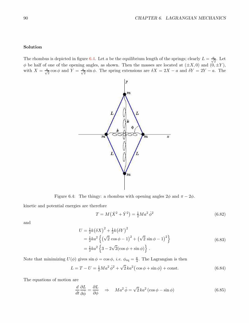
90 CHAPTER 6. LAGRANGIAN MECHANICS
Solution
The rhombus is depicted in figure 6.4. Let a be the equilibrium length of the springs; clearly L = a√2. Let
φ be half of one of the opening angles, as shown. Then the masses are located at (±X, 0) and (0,±Y ),with X = a√
2cosφ and Y = a√
2sinφ. The spring extensions are δX = 2X − a and δY = 2Y − a. The
Figure 6.4: The thingy: a rhombus with opening angles 2φ and π − 2φ.
kinetic and potential energies are therefore
T =M(X2 + Y 2
)= 1
2Ma2 φ2 (6.82)
and
U = 12k(δX)2
+ 12k(δY)2
= 12ka
2(√
2 cosφ− 1)2
+(√
2 sinφ− 1)2
= 12ka
23− 2
√2(cos φ+ sinφ)
.
(6.83)
Note that minimizing U(φ) gives sinφ = cosφ, i.e. φeq = π4 . The Lagrangian is then
L = T − U = 12Ma2 φ2 +
√2 ka2
(cosφ+ sinφ
)+ const. (6.84)
The equations of motion are
d
dt
∂L
∂φ=∂L
∂φ⇒ Ma2 φ =
√2 ka2 (cosφ− sinφ) (6.85)

6.7. APPENDIX : VIRIAL THEOREM 91
It’s always smart to expand about equilibrium, so let’s write φ = π4 + δ, which leads to
δ + ω20 sin δ = 0 , (6.86)
with ω0 =√
2k/M . This is the equation of a pendulum! Linearizing gives δ + ω20 δ = 0, so the small
oscillation frequency is just ω0.
6.7 Appendix : Virial Theorem
The virial theorem is a statement about the time-averaged motion of a mechanical system. Define thevirial ,
G(q, p) =∑
σ
pσ qσ . (6.87)
Then
dG
dt=∑
σ
(pσ qσ + pσ qσ
)
=∑
σ
qσ Fσ +∑
σ
qσ∂L
∂qσ. (6.88)
Now suppose that T = 12
∑σ,σ′ Tσσ′ qσqσ′ is homogeneous of degree k = 2 in q, and that U is homogeneous
of degree zero in q. Then ∑
σ
qσ∂L
∂qσ=∑
σ
qσ∂T
∂qσ= 2T, (6.89)
which follows from Euler’s theorem on homogeneous functions.
Now consider the time average of G over a period τ :
⟨dGdt
⟩=
1
τ
τ∫
0
dtdG
dt
=1
τ
[G(τ) −G(0)
]. (6.90)
If G(t) is bounded, then in the limit τ → ∞ we must have 〈G〉 = 0. Any bounded motion, such as the
orbit of the earth around the Sun, will result in 〈G〉τ→∞ = 0. But then
⟨dGdt
⟩= 2 〈T 〉+
⟨∑
σ
qσ Fσ
⟩= 0 , (6.91)
which implies
〈T 〉 = −12
⟨∑
σ
qσ Fσ
⟩= +
⟨12
∑
σ
qσ∂U
∂qσ
⟩
=⟨12
∑
i
ri ·∇iU(r1, . . . , rN
)⟩
= 12k 〈U〉 ,
(6.92)

92 CHAPTER 6. LAGRANGIAN MECHANICS
where the last line pertains to homogeneous potentials of degree k. Finally, since T +U = E is conserved,we have
〈T 〉 = k E
k + 2, 〈U〉 = 2E
k + 2. (6.93)

Chapter 7
Noether’s Theorem
7.1 Continuous Symmetry Implies Conserved Charges
Consider a particle moving in two dimensions under the influence of an external potential U(r). Thepotential is a function only of the magnitude of the vector r. The Lagrangian is then
L = T − U = 12m(r2 + r2 φ2
)− U(r) , (7.1)
where we have chosen generalized coordinates (r, φ). The momentum conjugate to φ is pφ = mr2 φ. The
generalized force Fφ clearly vanishes, since L does not depend on the coordinate φ. (One says that L is‘cyclic’ in φ.) Thus, although r = r(t) and φ = φ(t) will in general be time-dependent, the combination
pφ = mr2 φ is constant. This is the conserved angular momentum about the z axis.
If instead the particle moved in a potential U(y), independent of x, then writing
L = 12m(x2 + y2
)− U(y) , (7.2)
we have that the momentum px = ∂L/∂x = mx is conserved, because the generalized force Fx = ∂L/∂x =0 vanishes. This situation pertains in a uniform gravitational field, with U(x, y) = mgy, independent ofx. The horizontal component of momentum is conserved.
In general, whenever the system exhibits a continuous symmetry , there is an associated conserved charge.(The terminology ‘charge’ is from field theory.) Indeed, this is a rigorous result, known as Noether’s
Theorem. Consider a one-parameter family of transformations,
qσ −→ qσ(q, ζ) , (7.3)
where ζ is the continuous parameter. Suppose further (without loss of generality) that at ζ = 0 thistransformation is the identity, i.e. qσ(q, 0) = qσ. The transformation may be nonlinear in the generalizedcoordinates. Suppose further that the Lagrangian L is invariant under the replacement q → q. Then we
93

94 CHAPTER 7. NOETHER’S THEOREM
must have
0 =d
dζ
∣∣∣∣∣ζ=0
L(q, ˙q, t) =∂L
∂qσ
∂qσ∂ζ
∣∣∣∣∣ζ=0
+∂L
∂qσ
∂ ˙qσ∂ζ
∣∣∣∣∣ζ=0
=d
dt
(∂L
∂qσ
)∂qσ∂ζ
∣∣∣∣∣ζ=0
+∂L
∂qσ
d
dt
(∂qσ∂ζ
)
ζ=0
=d
dt
(∂L
∂qσ
∂qσ∂ζ
)
ζ=0
. (7.4)
Thus, there is an associated conserved charge
Λ =∂L
∂qσ
∂qσ∂ζ
∣∣∣∣∣ζ=0
. (7.5)
7.1.1 Examples of one-parameter families of transformations
Consider the LagrangianL = 1
2m(x2 + y2)− U(√
x2 + y2). (7.6)
In two-dimensional polar coordinates, we have
L = 12m(r2 + r2φ2)− U(r) , (7.7)
and we may now define
r(ζ) = r
φ(ζ) = φ+ ζ .(7.8)
Note that r(0) = r and φ(0) = φ, i.e. the transformation is the identity when ζ = 0. We now have
Λ =∑
σ
∂L
∂qσ
∂qσ∂ζ
∣∣∣∣∣ζ=0
=∂L
∂r
∂r
∂ζ
∣∣∣∣∣ζ=0
+∂L
∂φ
∂φ
∂ζ
∣∣∣∣∣ζ=0
= mr2φ . (7.9)
Another way to derive the same result which is somewhat instructive is to work out the transformationin Cartesian coordinates. We then have
x(ζ) = x cos ζ − y sin ζ
y(ζ) = x sin ζ + y cos ζ .(7.10)
Thus,∂x
∂ζ= −y ,
∂y
∂ζ= x (7.11)
and
Λ =∂L
∂x
∂x
∂ζ
∣∣∣∣∣ζ=0
+∂L
∂y
∂y
∂ζ
∣∣∣∣∣ζ=0
= m(xy − yx) . (7.12)

7.1. CONTINUOUS SYMMETRY IMPLIES CONSERVED CHARGES 95
Butm(xy − yx) = mz · r × r = mr2φ . (7.13)
As another example, consider the potential
U(ρ, φ, z) = V (ρ, aφ+ z) , (7.14)
where (ρ, φ, z) are cylindrical coordinates for a particle of mass m, and where a is a constant withdimensions of length. The Lagrangian is
12m(ρ2 + ρ2φ2 + z2
)− V (ρ, aφ+ z) . (7.15)
This model possesses a helical symmetry, with a one-parameter family
ρ(ζ) = ρ
φ(ζ) = φ+ ζ
z(ζ) = z − ζa .
(7.16)
Note thataφ+ z = aφ+ z , (7.17)
so the potential energy, and the Lagrangian as well, is invariant under this one-parameter family oftransformations. The conserved charge for this symmetry is
Λ =∂L
∂ρ
∂ρ
∂ζ
∣∣∣∣∣ζ=0
+∂L
∂φ
∂φ
∂ζ
∣∣∣∣∣ζ=0
+∂L
∂z
∂z
∂ζ
∣∣∣∣∣ζ=0
= mρ2φ−maz . (7.18)
We can check explicitly that Λ is conserved, using the equations of motion
d
dt
(∂L
∂φ
)=
d
dt
(mρ2φ
)=∂L
∂φ= −a∂V
∂z
d
dt
(∂L
∂z
)=
d
dt(mz) =
∂L
∂z= −∂V
∂z.
(7.19)
Thus,
Λ =d
dt
(mρ2φ
)− a
d
dt(mz) = 0 . (7.20)
7.1.2 Conservation of Linear and Angular Momentum
Suppose that the Lagrangian of a mechanical system is invariant under a uniform translation of allparticles in the n direction. Then our one-parameter family of transformations is given by
xa = xa + ζ n , (7.21)
and the associated conserved Noether charge is
Λ =∑
a
∂L
∂xa· n = n · P , (7.22)

96 CHAPTER 7. NOETHER’S THEOREM
where P =∑
a pa is the total momentum of the system.
If the Lagrangian of a mechanical system is invariant under rotations about an axis n, then
xa = R(ζ, n)xa
= xa + ζ n× xa +O(ζ2) ,(7.23)
where we have expanded the rotation matrix R(ζ, n) in powers of ζ. The conserved Noether chargeassociated with this symmetry is
Λ =∑
a
∂L
∂xa· n× xa = n ·
∑
a
xa × pa = n · L , (7.24)
where L is the total angular momentum of the system.
7.1.3 Invariance of L vs. Invariance of S
Observant readers might object that demanding invariance of L is too strict. We should instead bedemanding invariance of the action S1. Suppose S is invariant under
t→ t(q, t, ζ)
qσ(t) → qσ(q, t, ζ) .(7.25)
Then invariance of S means
S =
tb∫
ta
dtL(q, q, t) =
tb∫
ta
dtL(q, ˙q, t) . (7.26)
Note that t is a dummy variable of integration, so it doesn’t matter whether we call it t or t. Theendpoints of the integral, however, do change under the transformation. Now consider an infinitesimaltransformation, for which δt = t− t and δq = q
(t)− q(t) are both small. Thus,
S =
tb∫
ta
dtL(q, q, t) =
tb+δtb∫
ta+δta
dtL(q, q, t) +
∂L
∂qσδqσ +
∂L
∂qσδqσ + . . .
, (7.27)
where
δqσ(t) ≡ qσ(t)− qσ(t)
= qσ(t)− qσ
(t)+ qσ(t)− qσ(t)
= δqσ − qσ δt+O(δq δt)
(7.28)
1Indeed, we should be demanding that S only change by a function of the endpoint values.

7.2. THE HAMILTONIAN 97
Subtracting eqn. 7.27 from eqn. 7.26, we obtain
0 = Lb δtb − La δta +∂L
∂qσ
∣∣∣∣b
δqσ,b −∂L
∂qσ
∣∣∣∣a
δqσ,a +
tb+δtb∫
ta+δta
dt
∂L
∂qσ− d
dt
(∂L
∂qσ
)δqσ(t)
=
tb∫
ta
dtd
dt
(L− ∂L
∂qσqσ
)δt+
∂L
∂qσδqσ
,
(7.29)
where La,b is L(q, q, t) evaluated at t = ta,b. Thus, if ζ ≡ δζ is infinitesimal, and
δt = A(q, t) δζ
δqσ = Bσ(q, t) δζ ,(7.30)
then the conserved charge is
Λ =
(L− ∂L
∂qσqσ
)A(q, t) +
∂L
∂qσBσ(q, t)
= −H(q, p, t)A(q, t) + pσ Bσ(q, t) .
(7.31)
Thus, when A = 0, we recover our earlier results, obtained by assuming invariance of L. Note thatconservation of H follows from time translation invariance: t→ t+ ζ, for which A = 1 and Bσ = 0. Herewe have written
H = pσ qσ − L , (7.32)
and expressed it in terms of the momenta pσ, the coordinates qσ, and time t. H is called the Hamiltonian.
7.2 The Hamiltonian
The Lagrangian is a function of generalized coordinates, velocities, and time. The canonical momentumconjugate to the generalized coordinate qσ is
pσ =∂L
∂qσ. (7.33)
The Hamiltonian is a function of coordinates, momenta, and time. It is defined as the Legendre transformof L:
H(q, p, t) =∑
σ
pσ qσ − L . (7.34)
Let’s examine the differential of H:
dH =∑
σ
(qσ dpσ + pσ dqσ − ∂L
∂qσdqσ − ∂L
∂qσdqσ
)− ∂L
∂tdt
=∑
σ
(qσ dpσ − ∂L
∂qσdqσ
)− ∂L
∂tdt ,
(7.35)

98 CHAPTER 7. NOETHER’S THEOREM
where we have invoked the definition of pσ to cancel the coefficients of dqσ. Since pσ = ∂L/∂qσ, we haveHamilton’s equations of motion,
qσ =∂H
∂pσ, pσ = −∂H
∂qσ. (7.36)
Thus, we can write
dH =∑
σ
(qσ dpσ − pσ dqσ
)− ∂L
∂tdt . (7.37)
Dividing by dt, we obtaindH
dt= −∂L
∂t, (7.38)
which says that the Hamiltonian is conserved (i.e. it does not change with time) whenever there is noexplicit time dependence to L.
Example #1 : For a simple d = 1 system with L = 12mx
2 − U(x), we have p = mx and
H = p x− L = 12mx
2 + U(x) =p2
2m+ U(x) . (7.39)
Example #2 : Consider now the mass point – wedge system analyzed above, with
L = 12(M +m)X2 +mXx+ 1
2m (1 + tan2α) x2 −mg x tanα , (7.40)
The canonical momenta are
P =∂L
∂X= (M +m) X +mx (7.41)
p =∂L
∂x= mX +m (1 + tan2α) x . (7.42)
The Hamiltonian is given by
H = P X + p x− L
= 12(M +m)X2 +mXx+ 1
2m (1 + tan2α) x2 +mg x tanα . (7.43)
However, this is not quite H, since H = H(X,x, P, p, t) must be expressed in terms of the coordinatesand the momenta and not the coordinates and velocities. So we must eliminate X and x in favor of Pand p. We do this by inverting the relations
(Pp
)=
(M +m mm m (1 + tan2α)
)(Xx
)(7.44)
to obtain (Xx
)=
1
m(M + (M +m) tan2α
)(m (1 + tan2α) −m
−m M +m
)(Pp
). (7.45)
Substituting into 7.43, we obtain
H =M +m
2m
P 2 cos2α
M +m sin2α− Pp cos2α
M +m sin2α+
p2
2 (M +m sin2α)+mg x tanα . (7.46)
Notice that P = 0 since ∂L∂X = 0. P is the total horizontal momentum of the system (wedge plus particle)
and it is conserved.

7.2. THE HAMILTONIAN 99
7.2.1 Is H = T + U ?
The most general form of the kinetic energy is
T = T2 + T1 + T0
= 12T
(2)σσ′(q, t) qσ qσ′ + T (1)
σ (q, t) qσ + T (0)(q, t) ,
where T (n)(q, q, t) is homogeneous of degree n in the velocities2 . We assume a potential energy of theform
U = U1 + U0
= U (1)σ (q, t) qσ + U (0)(q, t) , (7.47)
which allows for velocity-dependent forces, as we have with charged particles moving in an electromagneticfield. The Lagrangian is then
L = T − U = 12T
(2)σσ′(q, t) qσ qσ′ + T (1)
σ (q, t) qσ + T (0)(q, t)− U (1)σ (q, t) qσ − U (0)(q, t) . (7.48)
The canonical momentum conjugate to qσ is
pσ =∂L
∂qσ= T
(2)σσ′ qσ′ + T (1)
σ (q, t)− U (1)σ (q, t) (7.49)
which is inverted to give
qσ = T(2)σσ′
−1 (pσ′ − T
(1)σ′ + U
(1)σ′
). (7.50)
The Hamiltonian is then
H = pσ qσ − L
= 12 T
(2)σσ′
−1(pσ − T (1)
σ + U (1)σ
)(pσ′ − T
(1)σ′ + U
(1)σ′
)− T0 + U0
= T2 − T0 + U0 .
(7.51)
If T0, T1, and U1 vanish, i.e. if T (q, q, t) is a homogeneous function of degree two in the generalizedvelocities, and U(q, t) is velocity-independent, then H = T + U . But if T0 or T1 is nonzero, or thepotential is velocity-dependent, then H 6= T + U .
7.2.2 Example: A bead on a rotating hoop
Consider a bead of mass m constrained to move along a hoop of radius a. The hoop is further constrainedto rotate with angular velocity φ = ω about the z-axis, as shown in Fig. 7.1.
2A homogeneous function of degree k satisfies f(λx1, . . . , λxn) = λkf(x1, . . . , xn). It is then easy to prove Euler’s theorem,∑ni=1 xi
∂f∂xi
= kf .

100 CHAPTER 7. NOETHER’S THEOREM
Figure 7.1: A bead of mass m on a rotating hoop of radius a.
The most convenient set of generalized coordinates is spherical polar (r, θ, φ), in which case
T = 12m(r2 + r2 θ2 + r2 sin2 θ φ2
)
= 12ma
2(θ2 + ω2 sin2 θ
).
(7.52)
Thus, T2 = 12ma
2θ2 and T0 = 12ma
2ω2 sin2 θ. The potential energy is U(θ) = mga(1 − cos θ). The
momentum conjugate to θ is pθ = ma2θ, and thus
H(θ, p) = T2 − T0 + U
= 12ma
2θ2 − 12ma
2ω2 sin2 θ +mga(1 − cos θ)
=p2θ
2ma2− 1
2ma2ω2 sin2 θ +mga(1− cos θ) .
(7.53)
For this problem, we can define the effective potential
Ueff(θ) ≡ U − T0 = mga(1 − cos θ)− 12ma
2ω2 sin2 θ
= mga(1− cos θ − ω2
2ω20
sin2 θ),
(7.54)
where ω20 ≡ g/a. The Lagrangian may then be written
L = 12ma
2θ2 − Ueff(θ) , (7.55)
and thus the equations of motion are
ma2θ = −∂Ueff
∂θ. (7.56)
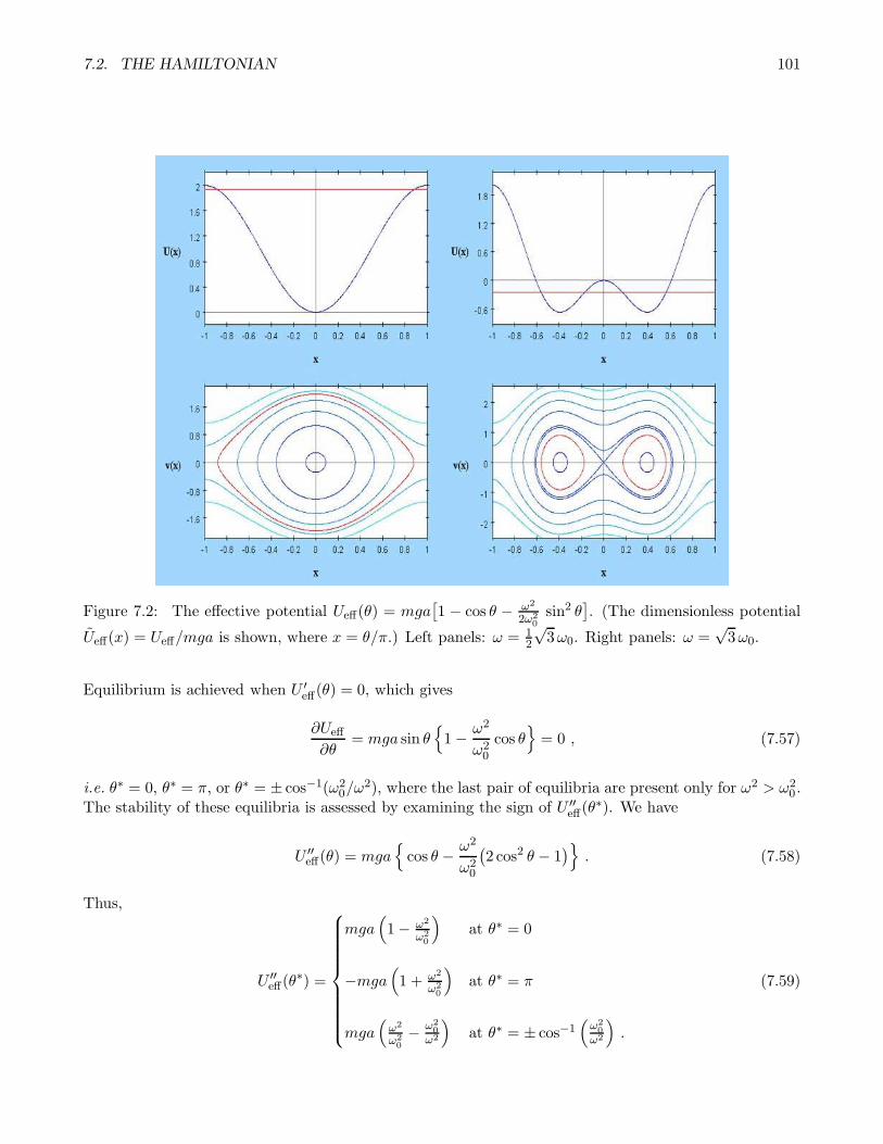
7.2. THE HAMILTONIAN 101
Figure 7.2: The effective potential Ueff(θ) = mga[1 − cos θ − ω2
2ω20sin2 θ
]. (The dimensionless potential
Ueff(x) = Ueff/mga is shown, where x = θ/π.) Left panels: ω = 12
√3ω0. Right panels: ω =
√3ω0.
Equilibrium is achieved when U ′eff(θ) = 0, which gives
∂Ueff
∂θ= mga sin θ
1− ω2
ω20
cos θ= 0 , (7.57)
i.e. θ∗ = 0, θ∗ = π, or θ∗ = ± cos−1(ω20/ω
2), where the last pair of equilibria are present only for ω2 > ω20 .
The stability of these equilibria is assessed by examining the sign of U ′′eff(θ
∗). We have
U ′′eff(θ) = mga
cos θ − ω2
ω20
(2 cos2 θ − 1
). (7.58)
Thus,
U ′′eff(θ
∗) =
mga(1− ω2
ω20
)at θ∗ = 0
−mga(1 + ω2
ω20
)at θ∗ = π
mga(ω2
ω20− ω2
0ω2
)at θ∗ = ± cos−1
(ω20
ω2
).
(7.59)

102 CHAPTER 7. NOETHER’S THEOREM
Thus, θ∗ = 0 is stable for ω2 < ω20 but becomes unstable when the rotation frequency ω is sufficiently
large, i.e. when ω2 > ω20. In this regime, there are two new equilibria, at θ∗ = ± cos−1(ω2
0/ω2), which are
both stable. The equilibrium at θ∗ = π is always unstable, independent of the value of ω. The situationis depicted in Fig. 7.2.
7.2.3 Charged Particle in a Magnetic Field
Consider next the case of a charged particle moving in the presence of an electromagnetic field. Theparticle’s potential energy is
U(r, r) = q φ(r, t)− q
cA(r, t) · r , (7.60)
which is velocity-dependent. The kinetic energy is T = 12m r
2, as usual. Here φ(r) is the scalar potentialand A(r) the vector potential. The electric and magnetic fields are given by
E = −∇φ− 1
c
∂A
∂t, B = ∇×A . (7.61)
The canonical momentum is
p =∂L
∂r= m r +
q
cA , (7.62)
and hence the Hamiltonian is
H(r,p, t) = p · r − L
= mr2 +q
cA · r − 1
2m r2 − q
cA · r + q φ
= 12m r
2 + q φ
=1
2m
(p− q
cA(r, t)
)2+ q φ(r, t) .
(7.63)
If A and φ are time-independent, then H(r,p) is conserved.
Let’s work out the equations of motion. We have
d
dt
(∂L
∂r
)=∂L
∂r(7.64)
which gives
m r +q
c
dA
dt= −q∇φ+
q
c∇(A · r) , (7.65)
or, in component notation,
mxi +q
c
∂Ai
∂xjxj +
q
c
∂Ai
∂t= −q ∂φ
∂xi+q
c
∂Aj
∂xixj , (7.66)
which is to say
mxi = −q ∂φ∂xi
− q
c
∂Ai
∂t+q
c
(∂Aj
∂xi− ∂Ai
∂xj
)xj . (7.67)

7.3. FAST PERTURBATIONS : RAPIDLY OSCILLATING FIELDS 103
It is convenient to express the cross product in terms of the completely antisymmetric tensor of rankthree, ǫijk:
Bi = ǫijk∂Ak
∂xj, (7.68)
and using the result
ǫijk ǫimn = δjm δkn − δjn δkm , (7.69)
we have ǫijk Bi = ∂j Ak − ∂k Aj , and
mxi = −q ∂φ∂xi
− q
c
∂Ai
∂t+q
cǫijk xj Bk , (7.70)
or, in vector notation,
m r = −q∇φ− q
c
∂A
∂t+q
cr × (∇×A)
= qE +q
cr ×B ,
(7.71)
which is, of course, the Lorentz force law.
7.3 Fast Perturbations : Rapidly Oscillating Fields
Consider a free particle moving under the influence of an oscillating force,
mq = F sinωt . (7.72)
The motion of the system is then
q(t) = qh(t)−F cosωt
mω2, (7.73)
where qh(t) = A+ Bt is the solution to the homogeneous (unforced) equation of motion. Note that the
amplitude of the response q − qh goes as ω−2 and is therefore small when ω is large.
Now consider a general n = 1 system, with
H(q, p, t) = H0(q, p) + V (q) cos(ωt) . (7.74)
We assume that ω is much greater than any natural oscillation frequency associated with H0. We separatethe motion q(t) and p(t) into slow and fast components:
q(t) = Q(t) + ζ(t)
p(t) = P (t) + π(t) ,
(7.75)

104 CHAPTER 7. NOETHER’S THEOREM
where ζ(t) and π(t) oscillate with the driving frequency ω. Since ζ and π will be small, we expandHamilton’s equations in these quantities:
Q+ ζ =∂H0
∂P+∂2H0
∂P 2π +
∂2H0
∂Q∂Pζ +
1
2
∂3H0
∂Q2 ∂Pζ2 +
∂3H0
∂Q∂P 2ζπ +
1
2
∂3H0
∂P 3π2 + . . .
P + π = −∂H0
∂Q− ∂2H0
∂Q2ζ − ∂2H0
∂Q∂Pπ − 1
2
∂3H0
∂Q3ζ2 − ∂3H0
∂Q2 ∂Pζπ − 1
2
∂3H0
∂Q∂P 2π2
− ∂V
∂Qcos(ωt)− ∂2V
∂Q2ζ cos(ωt)− . . . .
(7.76)
We now average over the fast degrees of freedom to obtain an equation of motion for the slow variablesQ and P , which we here carry to lowest nontrivial order in averages of fluctuating quantities:
Q = H0P + 1
2H0QQP 〈ζ2〉+H0
QPP 〈ζπ〉+ 12H
0PPP 〈π2〉
P = −H0Q − 1
2H0QQQ 〈ζ2〉 −H0
QQP 〈ζπ〉 − 12H
0QPP 〈π2〉 − VQQ 〈ζ cosωt〉 ,
(7.77)
where we now adopt the shorthand notation H0QQP = ∂3H0/∂2Q∂P , etc. The fast degrees of freedom
obey
ζ = H0QP ζ +H0
PP π
π = −H0QQ ζ −H0
QP π − VQ cos(ωt) .(7.78)
We can solve these by replacing VQ cosωt above with VQ e−iωt, and writing ζ(t) = ζ0 e
−iωt and π(t) =
π0 e−iωt, resulting in (
H0QP + iω H0
PP
−H0QQ −H0
QP + iω
)(ζ0π0
)=
(0VQ
). (7.79)
We now invert the matrix to obtain ζ0 and π0, then take the real part, which yields
ζ(t) =H0
PP VQω2 + (H0
QP )2 −H0
QQH0PP
cosωt
π(t) = −H0
QP VQ
ω2 +H0QP
2 −H0QQH
0PP
cosωt−ω VQ
ω2 + (H0QP )
2 −H0QQH
0PP
sinωt .
(7.80)
Invoking⟨cos2(ωt)
⟩=⟨sin2(ωt)
⟩= 1
2 and⟨cos(ωt) sin(ωt)
⟩= 0, we substitute into Eqns. 7.77 to obtain
Q = H0P +
H0QQP (H0
PP )2 − 2H0
QPP H0QP H
0PP +H0
PPP (H0QP )
2 + ω2H0PPP
4(ω2 + (H0
QP )2 −H0
QQH0PP
)2 V 2Q (7.81)
and
P = −H0Q −
H0QQQ (H0
QP )2 = 2H0
QQP H0QP H
0PP +H0
QPP (H0QP )
2 + ω2H0QPP
4(ω2 + (H0
QP )2 −H0
QQH0PP
)2 V 2Q (7.82)
These equations may be written compactly as
Q =∂K
∂P, P = −∂K
∂Q, (7.83)

7.3. FAST PERTURBATIONS : RAPIDLY OSCILLATING FIELDS 105
where
K = H0 +14 H
0PP V
2Q
ω2 + (H0QP )
2 −H0QQH
0PP
. (7.84)
We are licensed only to retain the leading order term in the denominator, hence
K(Q,P ) = H0(Q,P ) +1
4ω2
∂2H0
∂P 2
(∂V
∂Q
)2. (7.85)
7.3.1 Example : pendulum with oscillating support
Consider a pendulum with a vertically oscillating point of support. The coordinates of the pendulumbob are
x = ℓ sin θ , y = a(t)− ℓ cos θ . (7.86)
The Lagrangian is easily obtained:
L = 12mℓ
2 θ2 +mℓa θ sin θ +mgℓ cos θ + 12ma
2 −mga
= 12mℓ
2 θ2 +m(g + a)ℓ cos θ+
these may be dropped︷ ︸︸ ︷12ma
2 −mga− d
dt
(mℓa cos θ
).
(7.87)
Thus we may take the Lagrangian to be
L = 12mℓ
2 θ2 +m(g + a)ℓ cos θ , (7.88)
from which we derive the Hamiltonian
H(θ, pθ, t) =p2θ
2mℓ2−mgℓ cos θ −mℓa cos θ
= H0(θ, pθ, t) + V1(θ) sinωt .
(7.89)
We have assumed a(t) = a0 sinωt, so
V1(θ) = mℓa0 ω2 cos θ . (7.90)
The effective Hamiltonian, per eqn. 7.85, is
K(θ, Pθ) =Pθ
2mℓ2−mgℓ cos θ + 1
4ma20 ω2 sin2 θ . (7.91)
Let’s define the dimensionless parameter
ǫ ≡ 2gℓ
ω2a20. (7.92)
The slow variable θ executes motion in the effective potential Veff(θ) = mgℓ v(θ), with
v(θ) = − cos θ +1
2ǫsin2 θ . (7.93)

106 CHAPTER 7. NOETHER’S THEOREM
Figure 7.3: Dimensionless potential v(θ) for ǫ = 1.5 (black curve) and ǫ = 0.5 (blue curve).
Differentiating, and dropping the bar on θ, we find that Veff(θ) is stationary when
v′(θ) = 0 ⇒ sin θ cos θ = −ǫ sin θ . (7.94)
Thus, θ = 0 and θ = π, where sin θ = 0, are equilibria. When ǫ < 1 (note ǫ > 0 always), there are twonew solutions, given by the roots of cos θ = −ǫ.
To assess stability of these equilibria, we compute the second derivative:
v′′(θ) = cos θ +1
ǫcos 2θ . (7.95)
From this, we see that θ = 0 is stable (i.e. v′′(θ = 0) > 0) always, but θ = π is stable for ǫ < 1 andunstable for ǫ > 1. When ǫ < 1, two new solutions appear, at cos θ = −ǫ, for which
v′′(cos−1(−ǫ)) = ǫ− 1
ǫ, (7.96)
which is always negative since ǫ < 1 in order for these equilibria to exist. The situation is sketched in fig.7.3, showing v(θ) for two representative values of the parameter ǫ. For ǫ > 1, the equilibrium at θ = πis unstable, but as ǫ decreases, a subcritical pitchfork bifurcation is encountered at ǫ = 1, and θ = πbecomes stable, while the outlying θ = cos−1(−ǫ) solutions are unstable.
7.4 Field Theory: Systems with Several Independent Variables
Suppose φa(x) depends on several independent variables: x1, x2, . . . , xn. Furthermore, suppose
S[φa(x)
]=
∫
Ω
dxL(φa ∂µφa,x) , (7.97)

7.4. FIELD THEORY: SYSTEMS WITH SEVERAL INDEPENDENT VARIABLES 107
i.e. the Lagrangian density L is a function of the fields φa and their partial derivatives ∂φa/∂xµ. Here Ωis a region in RK . Then the first variation of S is
δS =
∫
Ω
dx
∂L∂φa
δφa +∂L
∂(∂µφa)
∂ δφa∂xµ
=
∮
∂Ω
dΣ nµ∂L
∂(∂µφa)δφa +
∫
Ω
dx
∂L∂φa
− ∂
∂xµ
(∂L
∂(∂µφa)
)δφa ,
(7.98)
where ∂Ω is the (n−1)-dimensional boundary of Ω, dΣ is the differential surface area, and nµ is the unit
normal. If we demand ∂L/∂(∂µφa)∣∣∂Ω
= 0 or δφa∣∣∂Ω
= 0, the surface term vanishes, and we conclude
δS
δφa(x)=
∂L∂φa
− ∂
∂xµ
(∂L
∂(∂µφa)
). (7.99)
As an example, consider the case of a stretched string of linear mass density µ and tension τ . The actionis a functional of the height y(x, t), where the coordinate along the string, x, and time, t, are the twoindependent variables. The Lagrangian density is
L = 12µ
(∂y
∂t
)2
− 12τ
(∂y
∂x
)2
, (7.100)
whence the Euler-Lagrange equations are
0 =δS
δy(x, t)= − ∂
∂x
(∂L∂y′
)− ∂
∂t
(∂L∂y
)
= τ∂2y
∂x2− µ
∂2y
∂t2,
(7.101)
where y′ = ∂y∂x and y = ∂y
∂t . Thus, µy = τy′′, which is the Helmholtz equation. We’ve assumed boundary
conditions where δy(xa, t) = δy(xb, t) = δy(x, ta) = δy(x, tb) = 0.
The Lagrangian density for an electromagnetic field with sources is
L = − 116π Fµν F
µν − 1c jµA
µ . (7.102)
The equations of motion are then
∂L∂Aµ
− ∂
∂xν
(∂L
∂(∂µAν)
)= 0 ⇒ ∂µ F
µν =4π
cjν , (7.103)
which are Maxwell’s equations.
Recall the result of Noether’s theorem for mechanical systems:
d
dt
(∂L
∂qσ
∂qσ∂ζ
)
ζ=0
= 0 , (7.104)

108 CHAPTER 7. NOETHER’S THEOREM
where qσ = qσ(q, ζ) is a one-parameter (ζ) family of transformations of the generalized coordinates whichleaves L invariant. We generalize to field theory by replacing
qσ(t) −→ φa(x, t) , (7.105)
where φa(x, t) are a set of fields, which are functions of the independent variables x, y, z, t. We willadopt covariant relativistic notation and write for four-vector xµ = (ct, x, y, z). The generalization ofdΛ/dt = 0 is
∂
∂xµ
(∂L
∂ (∂µφa)
∂φa∂ζ
)
ζ=0
= 0 , (7.106)
where there is an implied sum on both µ and a. We can write this as ∂µ Jµ = 0, where
Jµ ≡ ∂L∂ (∂µφa)
∂φa∂ζ
∣∣∣∣∣ζ=0
. (7.107)
We call Λ = J0/c the total charge. If we assume J = 0 at the spatial boundaries of our system, thenintegrating the conservation law ∂µ J
µ over the spatial region Ω gives
dΛ
dt=
∫
Ω
d3x ∂0 J0 = −
∫
Ω
d3x∇ · J = −∮
∂Ω
dΣ n · J = 0 , (7.108)
assuming J = 0 at the boundary ∂Ω.
As an example, consider the case of a complex scalar field, with Lagrangian density3
L(ψ,ψ∗, ∂µψ, ∂µψ∗) = 1
2K (∂µψ∗)(∂µψ) − U
(ψ∗ψ
). (7.109)
This is invariant under the transformation ψ → eiζ ψ, ψ∗ → e−iζ ψ∗. Thus,
∂ψ
∂ζ= i eiζ ψ ,
∂ψ∗
∂ζ= −i e−iζ ψ∗ , (7.110)
and, summing over both ψ and ψ∗ fields, we have
Jµ =∂L
∂ (∂µψ)· (iψ) + ∂L
∂ (∂µψ∗)· (−iψ∗)
=K
2i
(ψ∗∂µψ − ψ ∂µψ∗) .
(7.111)
The potential, which depends on |ψ|2, is independent of ζ. Hence, this form of conserved 4-current isvalid for an entire class of potentials.
3We raise and lower indices using the Minkowski metric gµν = diag (+,−,−,−).

7.4. FIELD THEORY: SYSTEMS WITH SEVERAL INDEPENDENT VARIABLES 109
7.4.1 Gross-Pitaevskii model
As one final example of a field theory, consider the Gross-Pitaevskii model, with
L = i~ψ∗ ∂ψ
∂t− ~2
2m∇ψ∗ ·∇ψ − g
(|ψ|2 − n0
)2. (7.112)
This describes a Bose fluid with repulsive short-ranged interactions. Here ψ(x, t) is again a complexscalar field, and ψ∗ is its complex conjugate. Using the Leibniz rule, we have
δS[ψ∗, ψ] = S[ψ∗ + δψ∗, ψ + δψ]
=
∫dt
∫ddx
i~ψ∗ ∂δψ
∂t+ i~ δψ∗ ∂ψ
∂t− ~2
2m∇ψ∗ ·∇δψ − ~2
2m∇δψ∗ ·∇ψ
− 2g(|ψ|2 − n0
)(ψ∗δψ + ψδψ∗)
=
∫dt
∫ddx
[− i~
∂ψ∗
∂t+
~2
2m∇2ψ∗ − 2g
(|ψ|2 − n0
)ψ∗]δψ
+
[i~∂ψ
∂t+
~2
2m∇2ψ − 2g
(|ψ|2 − n0
)ψ
]δψ∗
,
where we have integrated by parts where necessary and discarded the boundary terms. ExtremizingS[ψ∗, ψ] therefore results in the nonlinear Schrodinger equation (NLSE),
i~∂ψ
∂t= − ~2
2m∇2ψ + 2g
(|ψ|2 − n0
)ψ (7.113)
as well as its complex conjugate,
− i~∂ψ∗
∂t= − ~2
2m∇2ψ∗ + 2g
(|ψ|2 − n0
)ψ∗ . (7.114)
Note that these equations are indeed the Euler-Lagrange equations:
δS
δψ=∂L∂ψ
− ∂
∂xµ
(∂L∂ ∂µψ
)
δS
δψ∗ =∂L∂ψ∗ − ∂
∂xµ
(∂L
∂ ∂µψ∗
),
(7.115)
with xµ = (t,x)4 Plugging in
∂L∂ψ
= −2g(|ψ|2 − n0
)ψ∗ ,
∂L∂ ∂tψ
= i~ψ∗ ,∂L∂∇ψ
= − ~2
2m∇ψ∗ (7.116)
and∂L∂ψ∗ = i~ψ − 2g
(|ψ|2 − n0
)ψ ,
∂L∂ ∂tψ∗ = 0 ,
∂L∂∇ψ∗ = − ~2
2m∇ψ , (7.117)
4In the nonrelativistic case, there is no utility in defining x0 = ct, so we simply define x0 = t.

110 CHAPTER 7. NOETHER’S THEOREM
we recover the NLSE and its conjugate.
The Gross-Pitaevskii model also possesses a U(1) invariance, under
ψ(x, t) → ψ(x, t) = eiζ ψ(x, t) , ψ∗(x, t) → ψ∗(x, t) = e−iζ ψ∗(x, t) . (7.118)
Thus, the conserved Noether current is then
Jµ =∂L∂ ∂µψ
∂ψ
∂ζ
∣∣∣∣∣ζ=0
+∂L
∂ ∂µψ∗∂ψ∗
∂ζ
∣∣∣∣∣ζ=0
J0 = −~ |ψ|2
J = − ~2
2im
(ψ∗
∇ψ − ψ∇ψ∗) .
(7.119)
Dividing out by ~, taking J0 ≡ −~ρ and J ≡ −~j, we obtain the continuity equation,
∂ρ
∂t+∇ · j = 0 , (7.120)
where
ρ = |ψ|2 , j =~
2im
(ψ∗
∇ψ − ψ∇ψ∗) . (7.121)
are the particle density and the particle current, respectively.
7.5 Hamiltonian Mechanics
Recall that L = L(q, q, t), and
pσ =∂L
∂qσ. (7.122)
The Hamiltonian, H(q, p) is obtained by a Legendre transformation,
H(q, p) =
n∑
σ=1
pσ qσ − L . (7.123)
Note that
dH =
n∑
σ=1
(pσ dqσ + qσ dpσ − ∂L
∂qσdqσ − ∂L
∂qσdqσ
)− ∂L
∂tdt
=
n∑
σ=1
(qσ dpσ − ∂L
∂qσdqσ
)− ∂L
∂tdt .
(7.124)
Thus, we obtain Hamilton’s equations of motion,
∂H
∂pσ= qσ ,
∂H
∂qσ= − ∂L
∂qσ= −pσ (7.125)

7.5. HAMILTONIAN MECHANICS 111
anddH
dt=∂H
∂t= −∂L
∂t. (7.126)
Some remarks:
• As an example, consider a particle moving in three dimensions, described by spherical polar coor-dinates (r, θ, φ). Then
L = 12m(r2 + r2 θ2 + r2 sin2θ φ2
)− U(r, θ, φ) . (7.127)
We have
pr =∂L
∂r= mr , pθ =
∂L
∂θ= mr2 θ , pφ =
∂L
∂φ= mr2 sin2θ φ , (7.128)
and thus
H = pr r + pθ θ + pφ φ− L
=p2r2m
+p2θ
2mr2+
p2φ
2mr2 sin2θ+ U(r, θ, φ) .
(7.129)
Note that H is time-independent, hence ∂H∂t = dH
dt = 0, and therefore H is a constant of the motion.
• In order to obtain H(q, p) we must invert the relation pσ = ∂L∂qσ
= pσ(q, q) to obtain qσ(q, p). Thisis possible if the Hessian,
∂pα∂qβ
=∂2L
∂qα ∂qβ(7.130)
is nonsingular. This is the content of the ‘inverse function theorem’ of multivariable calculus.
• Define the rank 2n vector, ξ, by its components,
ξi =
qi if 1 ≤ i ≤ n
pi−n if n < i ≤ 2n .(7.131)
Then we may write Hamilton’s equations compactly as
ξi = Jij∂H
∂ξj, (7.132)
where
J =
(On×n In×n
−In×n On×n
)(7.133)
is a rank 2n matrix. Note that Jt = −J, i.e. J is antisymmetric, and that J2 = −I2n×2n. We shallutilize this ‘symplectic structure’ to Hamilton’s equations shortly.

112 CHAPTER 7. NOETHER’S THEOREM
7.5.1 Modified Hamilton’s principle
We have that
0 = δ
tb∫
ta
dtL = δ
tb∫
ta
dt(pσ qσ −H
)
=
tb∫
ta
dt
pσ δqσ + qσ δpσ − ∂H
∂qσδqσ − ∂H
∂pσδpσ
=
tb∫
ta
dt
−(pσ +
∂H
∂qσ
)δqσ +
(qσ − ∂H
∂pσ
)δpσ
+(pσ δqσ
)∣∣∣tb
ta,
(7.134)
assuming δqσ(ta) = δqσ(tb) = 0. Setting the coefficients of δqσ and δpσ to zero, we recover Hamilton’sequations.
7.5.2 Phase flow is incompressible
A flow for which ∇ · v = 0 is incompressible – we shall see why in a moment. Let’s check that thedivergence of the phase space velocity does indeed vanish:
∇ · ξ =n∑
σ=1
∂qσ∂qσ
+∂pσ∂pσ
=
2n∑
i=1
∂ξi∂ξi
=∑
i,j
Jij∂2H
∂ξi ∂ξj= 0 .
(7.135)
Now let ρ(ξ, t) be a distribution on phase space. Continuity implies
∂ρ
∂t+∇ · (ρ ξ) = 0 . (7.136)
Invoking ∇ · ξ = 0, we have thatDρ
Dt=∂ρ
∂t+ ξ ·∇ρ = 0 , (7.137)
where Dρ/Dt is sometimes called the convective derivative – it is the total derivative of the functionρ(ξ(t), t
), evaluated at a point ξ(t) in phase space which moves according to the dynamics. This says
that the density in the “comoving frame” is locally constant.
7.5.3 Poincare recurrence theorem
Let gτ be the ‘τ -advance mapping’ which evolves points in phase space according to Hamilton’s equations
qσ = +∂H
∂pσ, pσ = − ∂H
∂qσ(7.138)

7.5. HAMILTONIAN MECHANICS 113
for a time interval ∆t = τ . Consider a region Ω in phase space. Define gnτΩ to be the nth image ofΩ under the mapping gτ . Clearly gτ is invertible; the inverse is obtained by integrating the equationsof motion backward in time. We denote the inverse of gτ by g−1
τ . By Liouville’s theorem, gτ is volumepreserving when acting on regions in phase space, since the evolution of any given point is Hamiltonian.This follows from the continuity equation for the phase space density,
∂
∂t+∇ · (u) = 0 (7.139)
where u = q, p is the velocity vector in phase space, and Hamilton’s equations, which say that thephase flow is incompressible, i.e. ∇ · u = 0:
∇ · u =
n∑
σ=1
∂qσ∂qσ
+∂pσ∂pσ
=
n∑
σ=1
∂
∂qσ
(∂H
∂pσ
)+
∂
∂pσ
(− ∂H
∂qσ
)= 0 . (7.140)
Thus, we have that the convective derivative vanishes, viz.
D
Dt≡ ∂
∂t+ u · ∇ = 0 , (7.141)
which guarantees that the density remains constant in a frame moving with the flow.
The proof of the recurrence theorem is simple. Assume that gτ is invertible and volume-preserving, asis the case for Hamiltonian flow. Further assume that phase space volume is finite. Since the energy ispreserved in the case of time-independent Hamiltonians, we simply ask that the volume of phase spaceat fixed total energy E be finite, i.e.
∫dµ δ
(E −H(q,p)
)<∞ , (7.142)
where dµ =∏
i dqi dpi is the phase space uniform integration measure.
Theorem: In any finite neighborhood Ω of phase space there exists a point ϕ0 which will return to Ωafter n applications of gτ , where n is finite.
Proof: Assume the theorem fails; we will show this assumption results in a contradiction. Consider theset Υ formed from the union of all sets gmτ Ω for all m:
Υ =
∞⋃
m=0
gmτ Ω (7.143)
We assume that the set gmτ Ω |m ∈ Z ,m ≥ 0 is disjoint. The volume of a union of disjoint sets is thesum of the individual volumes. Thus,
vol(Υ) =
∞∑
m=0
vol(gmτ Ω) = vol(Ω) ·∞∑
m=1
1 = ∞ , (7.144)
114 CHAPTER 7. NOETHER’S THEOREM
since vol(gmτ Ω) = vol(Ω) from volume preservation. But clearly Υ is a subset of the entire phase space,hence we have a contradiction, because by assumption phase space is of finite volume.
Thus, the assumption that the set gmτ Ω |m ∈ Z ,m ≥ 0 is disjoint fails. This means that there existssome pair of integers k and l, with k 6= l, such that gkτ Ω ∩ glτ Ω 6= ∅. Without loss of generality we mayassume k > l. Apply the inverse g−1
τ to this relation l times to get gk−lτ Ω∩Ω 6= ∅. Now choose any point
ϕ ∈ gnτ Ω ∩ Ω, where n = k − l, and define ϕ0 = g−nτ ϕ. Then by construction both ϕ0 and gnτ ϕ0 lie
within Ω and the theorem is proven.
Each of the two central assumptions – invertibility and volume preservation – is crucial. Without eitherof them, the proof fails. Consider, for example, a volume-preserving map which is not invertible. Anexample might be a mapping f : R → R which takes any real number to its fractional part. Thus,f(π) = 0.14159265 . . .. Let us restrict our attention to intervals of width less than unity. Clearly f isthen volume preserving. The action of f on the interval [2, 3) is to map it to the interval [0, 1). But [0, 1)remains fixed under the action of f , so no point within the interval [2, 3) will ever return under repeatediterations of f . Thus, f does not exhibit Poincare recurrence.
Consider next the case of the damped harmonic oscillator. In this case, phase space volumes contract.For a one-dimensional oscillator obeying x+2βx+Ω2
0x = 0 one has ∇·u = −2β < 0 (β > 0 for damping).
Thus the convective derivative is equal to Dt = −(∇·u) = +2β which says that the density increasesexponentially in the comoving frame, as (t) = e2βt (0). Thus, phase space volumes collapse, and arenot preserved by the dynamics. In this case, it is possible for the set Υ to be of finite volume, even if itis the union of an infinite number of sets gnτ Ω, because the volumes of these component sets themselvesdecrease exponentially, as vol(gnτ Ω) = e−2nβτ vol(Ω). A damped pendulum, released from rest at some
small angle θ0 , will not return arbitrarily close to these initial conditions.
7.5.4 Poisson brackets
The time evolution of any function F (q,p) over phase space is given by
d
dtF(q(t),p(t), t
)=∂F
∂t+
n∑
σ=1
∂F
∂qσqσ +
∂F
∂pσpσ
≡ ∂F
∂t+F,H
,
(7.145)
where the Poisson bracket · , · is given by
A,B
≡
n∑
σ=1
(∂A
∂qσ
∂B
∂pσ− ∂A
∂pσ
∂B
∂qσ
)
=
2n∑
i,j=1
Jij
∂A
∂ξi
∂B
∂ξj.
(7.146)
Properties of the Poisson bracket:
• Antisymmetry: f, g= −
g, f. (7.147)
7.6. CANONICAL TRANSFORMATIONS 115
• Bilinearity: if λ is a constant, and f , g, and h are functions on phase space, then
f + λ g, h
=f, h+ λg, h
. (7.148)
Linearity in the second argument follows from this and the antisymmetry condition.
• Associativity: fg, h
= f
g, h+ gf, h. (7.149)
• Jacobi identity: f, g, h
+g, h, f
+h, f, g
= 0 . (7.150)
Some other useful properties:
If A,H = 0 and ∂A∂t = 0, then dA
dt = 0 , i.e. A(q, p) is a constant of the motion.
If A,H = 0 and B,H = 0, thenA,B,H
= 0. If in addition A and B have no explicit time
dependence, we conclude that A,B is a constant of the motion.
It is easily established that
qα, qβ = 0 , pα, pβ = 0 , qα, pβ = δαβ . (7.151)
7.6 Canonical Transformations
7.6.1 Point transformations in Lagrangian mechanics
In Lagrangian mechanics, we are free to redefine our generalized coordinates, viz.
Qσ = Qσ(q1, . . . , qn, t) . (7.152)
This is called a “point transformation.” The transformation is invertible if
det
(∂Qα
∂qβ
)6= 0 . (7.153)
The transformed Lagrangian, L, written as a function of the new coordinates Q and velocities Q, is
L(Q, Q, t) = L
(q(Q, t), q(Q, Q, t), t
)+d
dtF(q(Q, t), t
), (7.154)
where F (q, t) is a function only of the coordinates qσ(Q, t) and time5. Finally, Hamilton’s principle,
δ
tb∫
t1
dt L(Q, Q, t) = 0 (7.155)
5We must have that the relation Qσ = Qσ(q, t) is invertible.

116 CHAPTER 7. NOETHER’S THEOREM
with δQσ(ta) = δQσ(tb) = 0, still holds, and the form of the Euler-Lagrange equations remains unchanged:
∂L
∂Qσ− d
dt
(∂L
∂Qσ
)= 0 . (7.156)
The invariance of the equations of motion under a point transformation may be verified explicitly. Wefirst evaluate
d
dt
(∂L
∂Qσ
)=
d
dt
(∂L
∂qα
∂qα
∂Qσ
)=
d
dt
(∂L
∂qα
∂qα∂Qσ
), (7.157)
where the relation ∂qα/∂Qσ = ∂qα/∂Qσ follows from qα = ∂qα∂Qσ
Qσ + ∂qα∂t . We know that adding a total
time derivative of a function F (Q, t) = F(q(Q, t), t
)to the Lagrangian does not alter the equations of
motion. Hence we can set F = 0 and compute
∂L
∂Qσ=
∂L
∂qα
∂qα∂Qσ
+∂L
∂qα
∂qα∂Qσ
=∂L
∂qα
∂qα∂Qσ
+∂L
∂qα
(∂2qα
∂Qσ ∂Qσ′
Qσ′ +∂2qα∂Qσ ∂t
)
=d
dt
(∂L
∂qσ
)∂qα∂Qσ
+∂L
∂qα
d
dt
(∂qα∂Qσ
)
=d
dt
(∂L
∂qσ
∂qα∂Qσ
)=
d
dt
(∂L
∂Qσ
),
(7.158)
where the last equality is what we obtained earlier in eqn. 7.157.
7.6.2 Canonical transformations in Hamiltonian mechanics
In Hamiltonian mechanics, we will deal with a much broader class of transformations – ones which mixall the q’s and p’s. The general form for a canonical transformation (CT) is
qσ = qσ(Q1, . . . , Qn ;P1, . . . , Pn; t
)
pσ = pσ(Q1, . . . , Qn ;P1, . . . , Pn; t
),
(7.159)
with σ ∈ 1, . . . , n. We may also write
ξi = ξi(Ξ1, . . . , Ξ2n; t
), (7.160)
with i ∈ 1, . . . , 2n. The transformed Hamiltonian is H(Q,P , t)., where, as we shall see below,H(Q,P , t) = H(q,p, t) + ∂
∂tF (q,Q, t).
What sorts of transformations are allowed? Well, if Hamilton’s equations are to remain invariant, then
Qσ =∂H
∂Pσ, Pσ = − ∂H
∂Qσ, (7.161)

7.6. CANONICAL TRANSFORMATIONS 117
which gives∂Qσ
∂Qσ+∂Pσ
∂Pσ= 0 =
∂Ξi
∂Ξi. (7.162)
I.e. the flow remains incompressible in the new (Q,P ) variables. We will also require that phase spacevolumes are preserved by the transformation, i.e.
det
(∂Ξi
∂ξj
)=
∣∣∣∣∣∣∣∣∂(Q,P )
∂(q,p)
∣∣∣∣∣∣∣∣ = 1 . (7.163)
Additional conditions will be discussed below.
7.6.3 Hamiltonian evolution
Hamiltonian evolution itself defines a canonical transformation. Let ξi = ξi(t) and let ξ′i = ξi(t + dt).
Then from the dynamics ξi = Jij ∂H/∂ξj , we have
ξi(t+ dt) = ξi(t) + Jij∂H
∂ξjdt+O
(dt2). (7.164)
Thus,
∂ξ′i∂ξj
=∂
∂ξj
(ξi + Jik
∂H
∂ξkdt+O
(dt2))
= δij + Jik
∂2H
∂ξj ∂ξkdt+O
(dt2).
(7.165)
Now, using the result det(1 + ǫM
)= 1 + ǫ Tr M +O(ǫ2) , we have
∣∣∣∣∣∣∣∣∂ξ′i∂ξj
∣∣∣∣∣∣∣∣ = 1 + Jjk
∂2H
∂ξj ∂ξkdt+O
(dt2)= 1 +O
(dt2). (7.166)
7.6.4 Symplectic structure
We have that
ξi = Jij
∂H
∂ξj. (7.167)
Suppose we make a time-independent canonical transformation to new phase space coordinates, Ξa =Ξa(ξ). We then have
Ξa =∂Ξa
∂ξjξj =
∂Ξa
∂ξjJjk
∂H
∂ξk. (7.168)
But if the transformation is canonical, then the equations of motion are preserved, and we also have
Ξa = Jab
∂H
∂Ξb= Jab
∂H
∂ξk
∂ξk∂Ξb
. (7.169)

118 CHAPTER 7. NOETHER’S THEOREM
Equating these two expressions, we have
Maj Jjk
∂H
∂ξk= JabM
−1kb
∂H
∂ξk, (7.170)
where Maj ≡ ∂Ξa/∂ξj is the Jacobian of the transformation. Since the equality must hold for all ξ, weconclude
MJ = J(M t)−1
=⇒ MJM t = J . (7.171)
A matrix M satisfying MM t = I is of course an orthogonal matrix. A matrix M satisfying MJM t = J
is called symplectic. We write M ∈ Sp(2n), i.e. M is an element of the group of symplectic matrices6 ofrank 2n.
The symplectic property of M guarantees that the Poisson brackets are preserved under a canonicaltransformation:
A,B
ξ= Jij
∂A
∂ξi
∂B
∂ξj= Jij
∂A
∂Ξa
∂Ξa
∂ξi
∂B
∂Ξb
∂Ξb
∂ξj
=(Mai Jij M
tjb
) ∂A∂Ξa
∂B
∂Ξb= Jab
∂A
∂Ξa
∂B
∂Ξb=A,B
Ξ.
(7.172)
7.6.5 Generating functions for canonical transformations
For a transformation to be canonical, we require
δ
tb∫
ta
dtpσ qσ −H(q,p, t)
= 0 = δ
tb∫
ta
dtPσ Qσ − H(Q,P , t)
. (7.173)
This is satisfied provided
pσ qσ −H(q,p, t)
= λ
Pσ Qσ − H(Q,P , t) +
dF
dt
, (7.174)
where λ is a constant. For canonical transformations7, λ = 1. Thus,
H(Q,P, t) = H(q, p, t) + Pσ Qσ − pσ qσ +∂F
∂qσqσ +
∂F
∂QσQσ
+∂F
∂pσpσ +
∂F
∂PσPσ +
∂F
∂t.
(7.175)
Thus, we require
∂F
∂qσ= pσ ,
∂F
∂Qσ= −Pσ ,
∂F
∂pσ= 0 ,
∂F
∂Pσ= 0 , (7.176)
6Note that the rank of a symplectic matrix is always even. Note also MJM t = J implies M tJM = J.
7Solutions of eqn. 7.174 with λ 6= 1 are known as extended canonical transformations. We can always rescale coordinatesand/or momenta to achieve λ = 1.

7.6. CANONICAL TRANSFORMATIONS 119
which says that F = F (q,Q, t) is only a function of (q,Q, t) and not a function of the momentumvariables p and P . The transformed Hamiltonian is then
H(Q,P , t) = H(q,p, t) +∂F (q,Q, t)
∂t. (7.177)
There are four possibilities, corresponding to the freedom to make Legendre transformations with respectto the coordinate arguments of F (q,Q, t) :
F (q,Q, t) =
F1(q,Q, t) ; pσ = +∂F1∂qσ
, Pσ = − ∂F1∂Qσ
(type I)
F2(q,P , t)− Pσ Qσ ; pσ = +∂F2∂qσ
, Qσ = + ∂F2∂Pσ
(type II)
F3(p,Q, t) + pσ qσ ; qσ = −∂F3∂pσ
, Pσ = − ∂F3∂Qσ
(type III)
F4(p,P , t) + pσ qσ − Pσ Qσ ; qσ = −∂F4∂pσ
, Qσ = + ∂F4∂Pσ
(type IV)
In each case (γ = 1, 2, 3, 4), we have
H(Q,P , t) = H(q,p, t) +∂Fγ
∂t. (7.178)
Let’s work out some examples:
• Consider the type-II transformation generated by
F2(q,P ) = Aσ(q)Pσ , (7.179)
where Aσ(q) is an arbitrary function of the qσ. We then have
Qσ =∂F2
∂Pσ= Aσ(q) , pσ =
∂F2
∂qσ=∂Aα
∂qσPα . (7.180)
Thus,
Qσ = Aσ(q) , Pσ =∂qα∂Qσ
pα . (7.181)
This is a general point transformation of the kind discussed in eqn. 7.152. For a general linear pointtransformation, Qα = Mαβ qβ, we have Pα = pβM
−1βα , i.e. Q = Mq, P = pM−1. If Mαβ = δαβ ,
this is the identity transformation. F2 = q1P3 + q3P1 interchanges labels 1 and 3, etc.
• Consider the type-I transformation generated by
F1(q,Q) = Aσ(q)Qσ . (7.182)
We then have
pσ =∂F1
∂qσ=∂Aα
∂qσQα
Pσ = − ∂F1
∂Qσ= −Aσ(q) .
(7.183)

120 CHAPTER 7. NOETHER’S THEOREM
Note that Aσ(q) = qσ generates the transformation
(q
p
)−→
(−P+Q
). (7.184)
• A mixed transformation is also permitted. For example,
F (q,Q) = q1Q1 + (q3 −Q2)P2 + (q2 −Q3)P3 (7.185)
is of type-I with respect to index σ = 1 and type-II with respect to indices σ = 2, 3. The transfor-mation effected is
Q1 = p1 , Q2 = q3 , Q3 = q2 , P1 = −q1 , P2 = p3 , P3 = p2 . (7.186)
• Consider the n = 1 harmonic oscillator,
H(q, p) =p2
2m+ 1
2kq2 . (7.187)
If we could find a time-independent canonical transformation such that
p =√
2mf(P ) cosQ , q =
√2 f(P )
ksinQ , (7.188)
where f(P ) is some function of P , then we’d have H(Q,P ) = f(P ), which is cyclic in Q. To findthis transformation, we take the ratio of p and q to obtain
p =√mk q ctnQ , (7.189)
which suggests the type-I transformation
F1(q,Q) = 12
√mk q2 ctnQ . (7.190)
This leads to
p =∂F1
∂q=
√mk q ctnQ , P = −∂F1
∂Q=
√mk q2
2 sin2Q. (7.191)
Thus,
q =
√2P
4√mk
sinQ =⇒ f(P ) =
√k
mP = ωP , (7.192)
where ω =√k/m is the oscillation frequency. We therefore have H(Q,P ) = ωP , whence P = E/ω.
The equations of motion are
P = −∂H∂Q
= 0 , Q =∂H
∂P= ω , (7.193)
which yields
Q(t) = ωt+ ϕ0 , q(t) =
√2E
mω2sin(ωt+ ϕ0
). (7.194)

Chapter 8
Constraints
A mechanical system of N point particles in d dimensions possesses n = dN degrees of freedom1. To spec-ify these degrees of freedom, we can choose any independent set of generalized coordinates q1, . . . , qK.Oftentimes, however, not all n coordinates are independent.
Consider, for example, the situation in Fig. 8.1, where a cylinder of radius a rolls over a half-cylinderof radius R. If there is no slippage, then the angles θ1 and θ2 are not independent, and they obey theequation of constraint ,
Rθ1 = a (θ2 − θ1) . (8.1)
In this case, we can easily solve the constraint equation and substitute θ2 =(1 + R
a
)θ1. In other cases,
though, the equation of constraint might not be so easily solved (e.g. it may be nonlinear). How then dowe proceed?
8.1 Constraints and Variational Calculus
Before addressing the subject of constrained dynamical systems, let’s consider the issue of constraints inthe broader context of variational calculus. Suppose we have a functional
F [y(x)] =
xb∫
xa
dxL(y, y′, x) , (8.2)
which we want to extremize subject to some constraints. Here y may stand for a set of functions yσ(x).There are two classes of constraints we will consider:
1For N rigid bodies, the number of degrees of freedom is n′ = 12d(d + 1)N , corresponding to d center-of-mass coordinates
and 12d(d− 1) angles of orientation for each particle. The dimension of the group of rotations in d dimensions is 1
2d(d− 1),
corresponding to the number of parameters in a general rank-d orthogonal matrix (i.e. an element of the group O(d)).
121
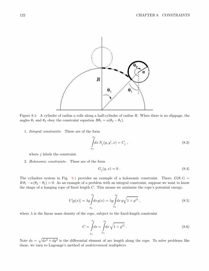
122 CHAPTER 8. CONSTRAINTS
Figure 8.1: A cylinder of radius a rolls along a half-cylinder of radius R. When there is no slippage, theangles θ1 and θ2 obey the constraint equation Rθ1 = a(θ2 − θ1).
1. Integral constraints: These are of the form
xb∫
xa
dxNj(y, y′, x) = Cj , (8.3)
where j labels the constraint.
2. Holonomic constraints: These are of the form
Gj(y, x) = 0 . (8.4)
The cylinders system in Fig. 8.1 provides an example of a holonomic constraint. There, G(θ, t) =Rθ1− a (θ2− θ1) = 0. As an example of a problem with an integral constraint, suppose we want to knowthe shape of a hanging rope of fixed length C. This means we minimize the rope’s potential energy,
U [y(x)] = λg
xb∫
xa
ds y(x) = λg
xb∫
xa
dx y
√1 + y′2 , (8.5)
where λ is the linear mass density of the rope, subject to the fixed-length constraint
C =
xb∫
xa
ds =
xb∫
xa
dx
√1 + y′2 . (8.6)
Note ds =√dx2 + dy2 is the differential element of arc length along the rope. To solve problems like
these, we turn to Lagrange’s method of undetermined multipliers.

8.2. CONSTRAINED EXTREMIZATION OF FUNCTIONS 123
8.2 Constrained Extremization of Functions
Given F (x1, . . . , xn) to be extremized subject to k constraints of the form Gj(x1, . . . , xn) = 0 wherej = 1, . . . , k, construct
F ∗(x1, . . . , xn;λ1, . . . , λk)≡ F (x1, . . . , xn) +
k∑
j=1
λj Gj(x1, . . . , xn) (8.7)
which is a function of the (n + k) variablesx1, . . . , xn;λ1, . . . , λk
. Now freely extremize the extended
function F ∗:
dF ∗ =n∑
σ=1
∂F ∗
∂xσdxσ +
k∑
j=1
∂F ∗
∂λjdλj
=
n∑
σ=1
∂F
∂xσ+
k∑
j=1
λj∂Gj
∂xσ
dxσ +
k∑
j=1
Gj dλj = 0
(8.8)
This results in the (n+ k) equations
∂F
∂xσ+
k∑
j=1
λj∂Gj
∂xσ= 0 (σ = 1, . . . , n)
Gj = 0 (j = 1, . . . , k) .
(8.9)
The interpretation of all this is as follows. The n equations in 8.9 can be written in vector form as
∇F +k∑
j=1
λj ∇Gj = 0 . (8.10)
This says that the (n-component) vector ∇F is linearly dependent upon the k vectors ∇Gj . Thus, anymovement in the direction of ∇F must necessarily entail movement along one or more of the directions∇Gj . This would require violating the constraints, since movement along ∇Gj takes us off the level
set Gj = 0. Were ∇F linearly independent of the set ∇Gj, this would mean that we could find a
differential displacement dx which has finite overlap with ∇F but zero overlap with each ∇Gj . Thus
x+ dx would still satisfy Gj(x+ dx) = 0, but F would change by the finite amount dF = ∇F (x) · dx.
8.3 Extremization of Functionals : Integral Constraints
Given a functional
F[yσ(x)
]=
xb∫
xa
dxL(yσ, y′σ, x
)(σ = 1, . . . , n) (8.11)

124 CHAPTER 8. CONSTRAINTS
subject to boundary conditions δyσ(xa) = δyσ(xb) = 0 and k constraints of the form
xb∫
xa
dxNl
(yσ, y′σ, x
)= Cl (l = 1, . . . , k) , (8.12)
construct the extended functional
F ∗[yσ(x); λj]≡
xb∫
xa
dx
L(yσ, y′σ, x
)+
k∑
l=1
λlNl
(yσ, y′σ, x
)−
k∑
l=1
λl Cl (8.13)
and freely extremize over y1, . . . , yn;λ1, . . . , λk. This results in (n+ k) equations
∂L
∂yσ− d
dx
(∂L
∂y′σ
)+
k∑
l=1
λl
∂Nl
∂yσ− d
dx
(∂Nl
∂y′σ
)= 0 (σ = 1, . . . , n)
xb∫
xa
dxNl
(yσ, y′σ, x
)= Cl (l = 1, . . . , k) .
(8.14)
8.4 Extremization of Functionals : Holonomic Constraints
Given a functional
F[yσ(x)
]=
xb∫
xa
dxL(yσ, y′σ, x
)(σ = 1, . . . , n) (8.15)
subject to boundary conditions δyσ(xa) = δyσ(xb) = 0 and k constraints of the form
Gj
(yσ(x), x
)= 0 (j = 1, . . . , k) , (8.16)
construct the extended functional
F ∗[yσ(x); λj(x)]≡
xb∫
xa
dx
L(yσ, y′σ, x
)+
k∑
j=1
λj Gj
(yσ
)(8.17)
and freely extremize overy1, . . . , yn;λ1, . . . , λk
:
δF ∗ =
xb∫
xa
dx
n∑
σ=1
(∂L
∂yσ− d
dx
(∂L
∂y′σ
)+
k∑
j=1
λj∂Gj
∂yσ
)δyσ +
k∑
j=1
Gj δλj
= 0 , (8.18)
resulting in the (n+ k) equations
d
dx
(∂L
∂y′σ
)− ∂L
∂yσ=
k∑
j=1
λj∂Gj
∂yσ(σ = 1, . . . , n)
Gj
(yσ, x
)= 0 (j = 1, . . . , k) .
(8.19)

8.4. EXTREMIZATION OF FUNCTIONALS : HOLONOMIC CONSTRAINTS 125
8.4.1 Examples of extremization with constraints
Volume of a cylinder : As a warm-up problem, let’s maximize the volume V = πa2h of a cylinder ofradius a and height h, subject to the constraint
G(a, h) = 2πa+h2
b− ℓ = 0 . (8.20)
We therefore define
V ∗(a, h, λ) ≡ V (a, h) + λG(a, h) , (8.21)
and set
∂V ∗
∂a= 2πah+ 2πλ = 0
∂V ∗
∂h= πa2 + 2λ
h
b= 0
∂V ∗
∂λ= 2πa+
h2
b− ℓ = 0 .
(8.22)
Solving these three equations simultaneously gives
a =2ℓ
5π, h =
√bℓ
5, λ =
2π
53/2b1/2 ℓ3/2 , V =
4
55/2 πℓ5/2 b1/2 . (8.23)
Hanging rope : We minimize the energy functional
E[y(x)
]= µg
x2∫
x1
dx y
√1 + y′2 , (8.24)
where µ is the linear mass density, subject to the constraint of fixed total length,
C[y(x)
]=
x2∫
x1
dx
√1 + y′2 . (8.25)
Thus,
E∗[y(x), λ]= E
[y(x)
]+ λC
[y(x)
]=
x2∫
x1
dxL∗(y, y′, x) , (8.26)
with
L∗(y, y′, x) = (µgy + λ)
√1 + y′2 . (8.27)
Since ∂L∗
∂x = 0 we have that
J = y′∂L∗
∂y′− L∗ = − µgy + λ√
1 + y′2(8.28)

126 CHAPTER 8. CONSTRAINTS
is constant. Thus,dy
dx= ±J −1
√(µgy + λ)2 − J 2 , (8.29)
with solution
y(x) = − λ
µg+
Jµg
cosh(µgJ (x− a)
). (8.30)
Here, J , a, and λ are constants to be determined by demanding y(xi) = yi (i = 1, 2), and that the totallength of the rope is C.
Geodesic on a curved surface : Consider next the problem of a geodesic on a curved surface. Let theequation for the surface be
G(x, y, z) = 0 . (8.31)
We wish to extremize the distance,
D =
b∫
a
ds =
b∫
a
√dx2 + dy2 + dz2 . (8.32)
We introduce a parameter t defined on the unit interval: t ∈ [0, 1], such that x(0) = xa, x(1) = xb, etc.Then D may be regarded as a functional, viz.
D[x(t), y(t), z(t)
]=
1∫
0
dt√x2 + y2 + z2 . (8.33)
We impose the constraint by forming the extended functional, D∗:
D∗[x(t), y(t), z(t), λ(t)]≡
1∫
0
dt
√x2 + y2 + z2 + λG(x, y, z)
, (8.34)
and we demand that the first functional derivatives of D∗ vanish:
δD∗
δx(t)= − d
dt
(x√
x2 + y2 + z2
)+ λ
∂G
∂x= 0
δD∗
δy(t)= − d
dt
(y√
x2 + y2 + z2
)+ λ
∂G
∂y= 0
δD∗
δz(t)= − d
dt
(z√
x2 + y2 + z2
)+ λ
∂G
∂z= 0
δD∗
δλ(t)= G(x, y, z) = 0 .
(8.35)
Thus,
λ(t) =vx− xv
v2 ∂xG=vy − yv
v2 ∂yG=vz − zv
v2 ∂zG, (8.36)
with v =√x2 + y2 + z2 and ∂x ≡ ∂
∂x , etc. These three equations are supplemented by G(x, y, z) = 0,which is the fourth.

8.5. APPLICATION TO MECHANICS 127
8.5 Application to Mechanics
Let us write our system of constraints in the differential form
n∑
σ=1
gjσ(q, t) dqσ + hj(q, t)dt = 0 (j = 1, . . . , k) . (8.37)
If the partial derivatives satisfy
∂gjσ∂qσ′
=∂gjσ′
∂qσ,
∂gjσ∂t
=∂hj∂qσ
, (8.38)
then the differential can be integrated to give dG(q, t) = 0, where
gjσ =∂Gj
∂qσ, hj =
∂Gj
∂t. (8.39)
The action functional is
S[qσ(t)] =tb∫
ta
dtL(qσ, qσ, t
)(σ = 1, . . . , n) , (8.40)
subject to boundary conditions δqσ(ta) = δqσ(tb) = 0. The first variation of S is given by
δS =
tb∫
ta
dt
n∑
σ=1
∂L
∂qσ− d
dt
(∂L
∂qσ
)δqσ . (8.41)
Since the qσ(t) are no longer independent, we cannot infer that the term in brackets vanishes for eachσ. What are the constraints on the variations δqσ(t)? The constraints are expressed in terms of virtualdisplacements which take no time: δt = 0. Thus,
n∑
σ=1
gjσ(q, t) δqσ(t) = 0 , (8.42)
where j = 1, . . . , k is the constraint index. We may now relax the constraint by introducing k undeter-mined functions λj(t), by adding integrals of the above equations with undetermined coefficient functionsto δS:
n∑
σ=1
∂L
∂qσ− d
dt
(∂L
∂qσ
)+
k∑
j=1
λj(t) gjσ(q, t)
δqσ(t) = 0 . (8.43)
Now we can demand that the term in brackets vanish for all σ. Thus, we obtain a set of (n+k) equations,
d
dt
(∂L
∂qσ
)− ∂L
∂qσ=
k∑
j=1
λj(t) gjσ(q, t) ≡ Qσ
gjσ(q, t) qσ + hj(q, t) = 0 ,
(8.44)

128 CHAPTER 8. CONSTRAINTS
in (n+k) unknownsq1, . . . , qn, λ1, . . . , λk
. Here, Qσ is the force of constraint conjugate to the generalized
coordinate qσ. Thus, with
pσ =∂L
∂qσ, Fσ =
∂L
∂qσ, Qσ =
k∑
j=1
λj gjσ , (8.45)
we write Newton’s second law as
pσ = Fσ +Qσ . (8.46)
Note that we can writeδS
δq(t)=∂L
∂q− d
dt
(∂L
∂q
)(8.47)
and that the instantaneous constraints may be written
gj · δq = 0 (j = 1, . . . , k) . (8.48)
Thus, by demanding
δS
δq(t)+
k∑
j=1
λj gj = 0 (8.49)
we require that the functional derivative be linearly dependent on the k vectors gj.
8.5.1 Constraints and conservation laws
We have seen how invariance of the Lagrangian with respect to a one-parameter family of coordinatetransformations results in an associated conserved quantity Λ, and how a lack of explicit time dependencein L results in the conservation of the Hamiltonian H. In deriving both these results, however, we usedthe equations of motion pσ = Fσ. What happens when we have constraints, in which case pσ = Fσ +Qσ?
Let’s begin with the Hamiltonian. We have H = qσ pσ − L, hence
dH
dt=
(pσ − ∂L
∂qσ
)qσ +
(pσ − ∂L
∂qσ
)qσ − ∂L
∂t
= Qσ qσ − ∂L
∂t.
(8.50)
We now use
Qσ qσ = λj gjσ qσ = −λj hj (8.51)
to obtaindH
dt= −λj hj −
∂L
∂t. (8.52)
We therefore conclude that in a system with constraints of the form gjσ qσ + hj = 0, the Hamiltonian is
conserved if each hj = 0 and if L is not explicitly dependent on time. In the case of holonomic constraints,
hj =∂Gj
∂t , so H is conserved if neither L nor any of the constraints Gj is explicitly time-dependent.

8.6. WORKED EXAMPLES 129
Next, let us rederive Noether’s theorem when constraints are present. We assume a one-parameter familyof transformations qσ → qσ(ζ) leaves L invariant. Then
0 =dL
dζ=
∂L
∂qσ
∂qσ∂ζ
+∂L
∂ ˙qσ
∂ ˙qσ∂ζ
=(˙pσ − Qσ
) ∂qσ∂ζ
+ pσd
dt
(∂qσ∂ζ
)
=d
dt
(pσ∂qσ∂ζ
)− λj gjσ
∂qσ∂ζ
.
(8.53)
Now let us write the constraints in differential form as
gjσ dqσ + hj dt+ kj dζ = 0 . (8.54)
We now havedΛ
dt= λj kj , (8.55)
which says that if the constraints are independent of ζ then Λ is conserved. For holonomic constraints,this means that
Gj
(q(ζ), t
)= 0 ⇒ kj =
∂Gj
∂ζ= 0 , (8.56)
i.e. Gj(q, t) has no explicit ζ dependence.
8.6 Worked Examples
Here we consider several example problems of constrained dynamics, and work each out in full detail.
8.6.1 One cylinder rolling off another
As an example of the constraint formalism, consider the system in Fig. 8.1, where a cylinder of radius arolls atop a cylinder of radius R. We have two constraints:
G1(r, θ1, θ2) = r −R− a = 0 (cylinders in contact)
G2(r, θ1, θ2) = Rθ1 − a (θ2 − θ1) = 0 (no slipping) ,(8.57)
from which we obtain the gjσ:
gjσ =
(1 0 00 R+ a −a
), (8.58)
which is to say
∂G1
∂r= 1 ,
∂G1
∂θ1= 0 ,
∂G1
∂θ2= 0 ,
∂G2
∂r= 0 ,
∂G2
∂θ1= R+ a ,
∂G2
∂θ2= −a . (8.59)

130 CHAPTER 8. CONSTRAINTS
The Lagrangian is
L = T − U = 12M(r2 + r2 θ21
)+ 1
2I θ22 −Mgr cos θ1 , (8.60)
where M and I are the mass and rotational inertia of the rolling cylinder, respectively. Note thatthe kinetic energy is a sum of center-of-mass translation Ttr = 1
2M(r2 + r2 θ21
)and rotation about the
center-of-mass, Trot =12I θ
22. The equations of motion are
d
dt
(∂L
∂r
)− ∂L
∂r=Mr −Mr θ21 +Mg cos θ1 = λ1 ≡ Qr
d
dt
(∂L
∂θ1
)− ∂L
∂θ1=Mr2θ1 + 2Mrr θ1 −Mgr sin θ1 = (R+ a)λ2 ≡ Qθ1
d
dt
(∂L
∂θ2
)− ∂L
∂θ2= Iθ2 = −aλ2 ≡ Qθ2
.
(8.61)
To these three equations we add the two constraints, resulting in five equations in the five unknownsr, θ1, θ2, λ1, λ2
.
We solve by first implementing the constraints, which give r = (R + a) a constant (i.e. r = 0), andθ2 =
(1 + R
a
)θ1. Substituting these into the above equations gives
−M(R+ a) θ21 +Mg cos θ1 = λ1
M(R + a)2θ1 −Mg(R + a) sin θ1 = (R + a)λ2
I
(R+ a
a
)θ1 = −aλ2 .
(8.62)
From the last of eqns. 8.62 we obtain
λ2 = −Iaθ2 = −R+ a
a2I θ1 , (8.63)
which we substitute into the second of eqns. 8.62 to obtain
(M +
I
a2
)(R+ a)2θ1 −Mg(R + a) sin θ1 = 0 . (8.64)
Multiplying by θ1, we obtain an exact differential, which may be integrated to yield
12M
(1 +
I
Ma2
)θ21 +
Mg
R+ acos θ1 =
Mg
R+ acos θ1 . (8.65)
Here, we have assumed that θ1 = 0 when θ1 = θ1, i.e. the rolling cylinder is released from rest at θ1 = θ1.Finally, inserting this result into the first of eqns. 8.62, we obtain the radial force of constraint,
Qr =Mg
1 + α
(3 + α) cos θ1 − 2 cos θ1
, (8.66)

8.6. WORKED EXAMPLES 131
Figure 8.2: Frictionless motion under gravity along a curved surface. The skier flies off the surface whenthe normal force vanishes.
where α = I/Ma2 is a dimensionless parameter (0 ≤ α ≤ 1). This is the radial component of the normal
force between the two cylinders. When Qr vanishes, the cylinders lose contact – the rolling cylinder fliesoff. Clearly this occurs at an angle θ1 = θ∗1, where
θ∗1 = cos−1
(2 cos θ13 + α
). (8.67)
The detachment angle θ∗1 is an increasing function of α, which means that larger I delays detachment.This makes good sense, since when I is larger the gain in kinetic energy is split between translationaland rotational motion of the rolling cylinder.
8.6.2 Frictionless motion along a curve
Consider the situation in Fig. 8.2 where a skier moves frictionlessly under the influence of gravity alonga general curve y = h(x). The Lagrangian for this problem is
L = 12m(x2 + y2)−mgy (8.68)
and the (holonomic) constraint isG(x, y) = y − h(x) = 0 . (8.69)
Accordingly, the Euler-Lagrange equations are
d
dt
(∂L
∂qσ
)− ∂L
∂qσ= λ
∂G
∂qσ, (8.70)
where q1 = x and q2 = y. Thus, we obtain
mx = −λh′(x) = Qx
my +mg = λ = Qy .(8.71)

132 CHAPTER 8. CONSTRAINTS
We eliminate y in favor of x by invoking the constraint. Since we need y, we must differentiate theconstraint, which gives
y = h′(x) x , y = h′(x) x+ h′′(x) x2 . (8.72)
Using the second Euler-Lagrange equation, we then obtain
λ
m= g + h′(x) x+ h′′(x) x2 . (8.73)
Finally, we substitute this into the first E-L equation to obtain an equation for x alone:(1 +
[h′(x)
]2)x+ h′(x)h′′(x) x2 + g h′(x) = 0 . (8.74)
Had we started by eliminating y = h(x) at the outset, writing
L(x, x) = 12m(1 +
[h′(x)
]2)x2 −mg h(x) , (8.75)
we would also have obtained this equation of motion.
The skier flies off the curve when the vertical force of constraint Qy = λ starts to become negative,because the curve can only supply a positive normal force. Suppose the skier starts from rest at a heighty0. We may then determine the point x at which the skier detaches from the curve by setting λ(x) = 0.To do so, we must eliminate x and x in terms of x. For x, we may use the equation of motion to write
x = −(gh′ + h′ h′′ x2
1 + h′2
), (8.76)
which allows us to write
λ = m
(g + h′′ x2
1 + h′2
). (8.77)
To eliminate x, we use conservation of energy,
E = mgy0 =12m(1 + h′
2)x2 +mgh , (8.78)
which fixes
x2 = 2g
(y0 − h
1 + h′2
). (8.79)
Putting it all together, we have
λ(x) =mg
(1 + h′2
)21 + h′
2+ 2(y0 − h)h′′
. (8.80)
The skier detaches from the curve when λ(x) = 0, i.e. when
1 + h′2+ 2(y0 − h)h′′ = 0 . (8.81)
There is a somewhat easier way of arriving at the same answer. This is to note that the skier must flyoff when the local centripetal force equals the gravitational force normal to the curve, i.e.
mv2(x)
R(x)= mg cos θ(x) , (8.82)

8.6. WORKED EXAMPLES 133
Figure 8.3: Finding the local radius of curvature: z = η2/2R.
where R(x) is the local radius of curvature. Now tan θ = h′, so cos θ =(1 + h′2
)−1/2. The square of
the velocity is v2 = x2 + y2 =(1 + h′2
)x2. What is the local radius of curvature R(x)? This can be
determined from the following argument, and from the sketch in Fig. 8.3. Writing x = x∗ + ǫ, we have
y = h(x∗) + h′(x∗) ǫ+ 12h
′′(x∗) ǫ2 + . . . . (8.83)
We now drop a perpendicular segment of length z from the point (x, y) to the line which is tangent tothe curve at
(x∗, h(x∗)
). According to Fig. 8.3, this means
(ǫy
)= η · 1√
1+h′2
(1h′
)− z · 1√
1+h′2
(−h′1
). (8.84)
Thus, we have
y = h′ ǫ+ 12h
′′ ǫ2
= h′(η + z h′√1 + h′2
)+ 1
2h′′(η + z h′√1 + h′2
)2
=η h′ + z h′2√
1 + h′2+
h′′ η2
2(1 + h′2
) +O(ηz)
=η h′ − z√1 + h′2
,
(8.85)
from which we obtain
z = − h′′ η2
2(1 + h′2
)3/2 +O(η3) (8.86)
and therefore
R(x) = − 1
h′′(x)·(1 +
[h′(x)
]2)3/2. (8.87)
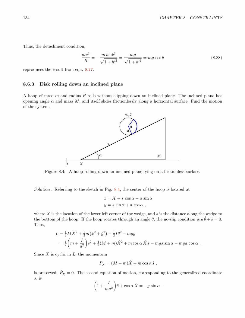
134 CHAPTER 8. CONSTRAINTS
Thus, the detachment condition,
mv2
R= − mh′′ x2√
1 + h′2=
mg√1 + h′2
= mg cos θ (8.88)
reproduces the result from eqn. 8.77.
8.6.3 Disk rolling down an inclined plane
A hoop of mass m and radius R rolls without slipping down an inclined plane. The inclined plane hasopening angle α and mass M , and itself slides frictionlessly along a horizontal surface. Find the motionof the system.
Figure 8.4: A hoop rolling down an inclined plane lying on a frictionless surface.
Solution : Referring to the sketch in Fig. 8.4, the center of the hoop is located at
x = X + s cosα− a sinα
y = s sinα+ a cosα ,
where X is the location of the lower left corner of the wedge, and s is the distance along the wedge tothe bottom of the hoop. If the hoop rotates through an angle θ, the no-slip condition is a θ+ s = 0.Thus,
L = 12MX2 + 1
2m(x2 + y2
)+ 1
2Iθ2 −mgy
= 12
(m+
I
a2
)s2 + 1
2 (M +m)X2 +m cosα X s−mgs sinα−mga cosα .
Since X is cyclic in L, the momentum
PX = (M +m)X +m cosα s ,
is preserved: PX = 0. The second equation of motion, corresponding to the generalized coordinates, is (
1 +I
ma2
)s+ cosα X = −g sinα .

8.6. WORKED EXAMPLES 135
Using conservation of PX , we eliminate s in favor of X, and immediately obtain
X =g sinα cosα(
1 + Mm
)(1 + I
ma2
)− cos2 α
≡ aX .
The result
s = −g(1 + M
m
)sinα
(1 + M
m
)(1 + I
ma2
)− cos2 α
≡ as
follows immediately. Thus,
X(t) = X(0) + X(0) t + 12aXt
2
s(t) = s(0) + s(0) t+ 12ast
2 .
Note that as < 0 while aX > 0, i.e. the hoop rolls down and to the left as the wedge slides to theright. Note that I = ma2 for a hoop; we’ve computed the answer here for general I.
8.6.4 Pendulum with nonrigid support
A particle of mass m is suspended from a flexible string of length ℓ in a uniform gravitational field. Whilehanging motionless in equilibrium, it is struck a horizontal blow resulting in an initial angular velocityω0. Treating the system as one with two degrees of freedom and a constraint, answer the following:
(a) Compute the Lagrangian, the equation of constraint, and the equations of motion.
Solution : The Lagrangian is
L = 12m(r2 + r2 θ2
)+mgr cos θ .
The constraint is r = ℓ. The equations of motion are
mr −mr θ2 −mg cos θ = λ
mr2 θ + 2mr r θ −mg sin θ = 0 .
(b) Compute the tension in the string as a function of angle θ.
Solution : Energy is conserved, hence
12mℓ
2 θ2 −mgℓ cos θ = 12mℓ
2 θ20 −mgℓ cos θ0 .
We take θ0 = 0 and θ0 = ω0. Thus,
θ2 = ω20 − 2Ω2
(1− cos θ
),
with Ω =√g/ℓ. Substituting this into the equation for λ, we obtain
λ = mg
2− 3 cos θ − ω2
0
Ω2
.

136 CHAPTER 8. CONSTRAINTS
(c) Show that if ω20 < 2g/ℓ then the particle’s motion is confined below the horizontal and that the
tension in the string is always positive (defined such that positive means exerting a pulling forceand negative means exerting a pushing force). Note that the difference between a string and a rigidrod is that the string can only pull but the rod can pull or push. Thus, the string tension must
always be positive or else the string goes “slack”.
Solution : Since θ2 ≥ 0, we must have
ω20
2Ω2≥ 1− cos θ .
The condition for slackness is λ = 0, or
ω20
2Ω2= 1− 3
2 cos θ .
Thus, if ω20 < 2Ω2, we have
1 >ω20
2Ω2> 1− cos θ > 1− 3
2 cos θ ,
and the string never goes slack. Note the last equality follows from cos θ > 0. The string rises to amaximum angle
θmax = cos−1(1− ω2
0
2Ω2
).
(d) Show that if 2g/ℓ < ω20 < 5g/ℓ the particle rises above the horizontal and the string becomes slack
(the tension vanishes) at an angle θ∗. Compute θ∗.
Solution : When ω2 > 2Ω2, the string rises above the horizontal and goes slack at an angle
θ∗ = cos−1(23 − ω2
0
3Ω2
).
This solution craps out when the string is still taut at θ = π, which means ω20 = 5Ω2.
(e) Show that if ω20 > 5g/ℓ the tension is always positive and the particle executes circular motion.
Solution : For ω20 > 5Ω2, the string never goes slack. Furthermore, θ never vanishes. Therefore,
the pendulum undergoes circular motion, albeit not with constant angular velocity.
8.6.5 Falling ladder
A uniform ladder of length ℓ and mass m has one end on a smooth horizontal floor and the other endagainst a smooth vertical wall. The ladder is initially at rest and makes an angle θ0 with respect to thehorizontal.
(a) Make a convenient choice of generalized coordinates and find the Lagrangian.

8.6. WORKED EXAMPLES 137
Figure 8.5: A ladder sliding down a wall and across a floor.
Solution : I choose as generalized coordinates the Cartesian coordinates (x, y) of the ladder’s centerof mass, and the angle θ it makes with respect to the floor. The Lagrangian is then
L = 12 m (x2 + y2) + 1
2 I θ2 +mgy .
There are two constraints: one enforcing contact along the wall, and the other enforcing contactalong the floor. These are written
G1(x, y, θ) = x− 12 ℓ cos θ = 0
G2(x, y, θ) = y − 12 ℓ sin θ = 0 .
(b) Prove that the ladder leaves the wall when its upper end has fallen to a height 23L sin θ0. The
equations of motion ared
dt
(∂L
∂qσ
)− ∂L
∂qσ=∑
j
λj∂Gj
∂qσ.
Thus, we have
mx = λ1 = Qx
my +mg = λ2 = Qy
I θ = 12ℓ(λ1 sin θ − λ2 cos θ
)= Qθ .
We now implement the constraints to eliminate x and y in terms of θ. We have
x = −12 ℓ sin θ θ x = −1
2 ℓ cos θ θ2 − 1
2 ℓ sin θ θ
y = 12 ℓ cos θ θ y = −1
2 ℓ sin θ θ2 + 1
2 ℓ cos θ θ .
We can now obtain the forces of constraint in terms of the function θ(t):
λ1 = −12mℓ
(sin θ θ + cos θ θ2
)
λ2 = +12mℓ
(cos θ θ − sin θ θ2
)+mg .

138 CHAPTER 8. CONSTRAINTS
We substitute these into the last equation of motion to obtain the result
I θ = −I0 θ − 12mgℓ cos θ ,
or
(1 + α) θ = −2ω20 cos θ ,
with I0 =14mℓ
2, α ≡ I/I0 and ω0 =√g/ℓ. This may be integrated once (multiply by θ to convert
to a total derivative) to yield
12(1 + α) θ2 + 2ω2
0 sin θ = 2ω20 sin θ0 ,
which is of course a statement of energy conservation. This,
θ2 =4ω2
0 (sin θ0 − sin θ)
1 + α
θ = −2ω20 cos θ
1 + α.
We may now obtain λ1(θ) and λ2(θ):
λ1(θ) = − mg
1 + α
(3 sin θ − 2 sin θ0
)cos θ
λ2(θ) =mg
1 + α
(3 sin θ − 2 sin θ0
)sin θ + α
.
Demanding λ1(θ) = 0 gives the detachment angle θ = θd, where
sin θd = 23 sin θ0 .
Note that λ2(θd) = mgα/(1 + α) > 0, so the normal force from the floor is always positive for
θ > θd. The time to detachment is
T1(θ0) =
∫dθ
θ=
√1 + α
2ω0
θ0∫
θd
dθ√sin θ0 − sin θ
.
(c) Show that the subsequent motion can be reduced to quadratures (i.e. explicit integrals).
Solution : After the detachment, there is no longer a constraint G1. The equations of motion are
mx = 0 (conservation of x-momentum)
my +mg = λ
I θ = −12 ℓ λ cos θ ,

8.6. WORKED EXAMPLES 139
along with the constraint y = 12 ℓ sin θ. Eliminating y in favor of θ using the constraint, the second
equation yieldsλ = mg − 1
2mℓ sin θ θ2 + 1
2mℓ cos θ θ .
Plugging this into the third equation of motion, we find
I θ = −2 I0 ω20 cos θ + I0 sin θ cos θ θ2 − I0 cos2 θ θ .
Multiplying by θ one again obtains a total time derivative, which is equivalent to rediscoveringenergy conservation:
E = 12
(I + I0 cos2 θ
)θ2 + 2 I0 ω
20 sin θ .
Figure 8.6: Plot of time to fall for the slipping ladder. Here x = sin θ0.
By continuity with the first phase of the motion, we obtain the initial conditions for this secondphase:
θ = sin−1(23 sin θ0
)
θ = −2ω0
√sin θ0
3 (1 + α).
Thus,
E = 12
(I + I0 − 4
9 I0 sin2 θ0)· 4ω
20 sin θ0
3 (1 + α)+ 1
3 mgℓ sin θ0
= 2 I0 ω20 ·1 + 4
27
sin2 θ01 + α
sin θ0 .

140 CHAPTER 8. CONSTRAINTS
(d) Find an expression for the time T (θ0) it takes the ladder to smack against the floor. Note that,
expressed in units of the time scale√L/g, T is a dimensionless function of θ0. Numerically integrate
this expression and plot T versus θ0.
Solution : The time from detachment to smack is
T2(θ0) =
∫dθ
θ=
1
2ω0
θd∫
0
dθ
√1 + α cos2 θ
(1− 4
27sin2 θ01+α
)sin θ0 − sin θ
.
The total time is then T (θ0) = T1(θ0) + T2(θ0). For a uniformly dense ladder, I = 112 mℓ
2 = 13 I0,
so α = 13 .
(e) What is the horizontal velocity of the ladder at long times?
Solution : From the moment of detachment, and thereafter,
x = −12 ℓ sin θ θ =
√4 g ℓ
27 (1 + α)sin3/2θ0 .
(f) Describe in words the motion of the ladder subsequent to it slapping against the floor.
Solution : Only a fraction of the ladder’s initial potential energy is converted into kinetic energy ofhorizontal motion. The rest is converted into kinetic energy of vertical motion and of rotation. Theslapping of the ladder against the floor is an elastic collision. After the collision, the ladder mustrise again, and continue to rise and fall ad infinitum, as it slides along with constant horizontalvelocity.
8.6.6 Point mass inside rolling hoop
Consider the point mass m inside the hoop of radius R, depicted in Fig. 8.7. We choose as generalizedcoordinates the Cartesian coordinates (X,Y ) of the center of the hoop, the Cartesian coordinates (x, y)for the point mass, the angle φ through which the hoop turns, and the angle θ which the point massmakes with respect to the vertical. These six coordinates are not all independent. Indeed, there are onlytwo independent coordinates for this system, which can be taken to be θ and φ. Thus, there are four
constraints:
X −Rφ ≡ G1 = 0
Y −R ≡ G2 = 0
x−X −R sin θ ≡ G3 = 0
y − Y +R cos θ ≡ G4 = 0 .
(8.89)
The kinetic and potential energies are easily expressed in terms of the Cartesian coordinates, aside fromthe energy of rotation of the hoop about its CM, which is expressed in terms of φ:
T = 12M(X2 + Y 2) + 1
2m(x2 + y2) + 12I φ
2
U =MgY +mgy . (8.90)

8.6. WORKED EXAMPLES 141
Figure 8.7: A point mass m inside a hoop of mass M , radius R, and moment of inertia I.
The moment of inertia of the hoop about its CM is I =MR2, but we could imagine a situation in whichI were different. For example, we could instead place the point mass inside a very short cylinder withtwo solid end caps, in which case I = 1
2MR2. The Lagrangian is then
L = 12M(X2 + Y 2) + 1
2m(x2 + y2) + 12I φ
2 −MgY −mgy . (8.91)
Note that L as written is completely independent of θ and θ!
Continuous symmetry
Note that there is an continuous symmetry to L which is satisfied by all the constraints, under
X(ζ) = X + ζ , Y (ζ) = Y
x(ζ) = x+ ζ , y(ζ) = y
φ(ζ) = φ+ζ
R, θ(ζ) = θ .
(8.92)
Thus, according to Noether’s theorem, there is a conserved quantity
Λ =∂L
∂X+∂L
∂x+
1
R
∂L
∂φ
=MX +mx+I
Rφ .
(8.93)
This means Λ = 0. This reflects the overall conservation of momentum in the x-direction.
Energy conservation
Since neither L nor any of the constraints are explicitly time-dependent, the Hamiltonian is conserved.And since T is homogeneous of degree two in the generalized velocities, we have H = E = T + U :
E = 12M(X2 + Y 2) + 1
2m(x2 + y2) + 12I φ
2 +MgY +mgy . (8.94)

142 CHAPTER 8. CONSTRAINTS
Equations of motion
We have n = 6 generalized coordinates and k = 4 constraints. Thus, there are four undeterminedmultipliers λ1, λ2, λ3, λ4 used to impose the constraints. This makes for ten unknowns:
X , Y , x , y , φ , θ , λ1 , λ2 , λ3 , λ4 . (8.95)
Accordingly, we have ten equations: six equations of motion plus the four equations of constraint. Theequations of motion are obtained from
d
dt
(∂L
∂qσ
)=
∂L
∂qσ+
k∑
j=1
λj∂Gj
∂qσ. (8.96)
Taking each generalized coordinate in turn, the equations of motion are thus
MX = λ1 − λ3
MY = −Mg + λ2 − λ4
mx = λ3
my = −mg + λ4
I φ = −Rλ10 = −R cos θ λ3 −R sin θ λ4 .
(8.97)
Along with the four constraint equations, these determine the motion of the system. Note that the lastof the equations of motion, for the generalized coordinate qσ = θ, says that Qθ = 0, which means that theforce of constraint on the point mass is radial. Were the point mass replaced by a rolling object, therewould be an angular component to this constraint in order that there be no slippage.
Implementation of constraints
We now use the constraint equations to eliminate X, Y , x, and y in terms of θ and φ:
X = Rφ , Y = R , x = Rφ+R sin θ , y = R(1− cos θ) . (8.98)
We also need the derivatives:
x = R φ+R cos θ θ , x = R φ+R cos θ θ −R sin θ θ2 , (8.99)
andy = R sin θ θ , y = R sin θ θ +R cos θ θ2 , (8.100)
as well asX = R φ , X = R φ , Y = 0 , Y = 0 . (8.101)
We now may write the conserved charge as
Λ =1
R(I +MR2 +mR2) φ+mR cos θ θ . (8.102)
8.6. WORKED EXAMPLES 143
This, in turn, allows us to eliminate φ in terms of θ and the constant Λ:
φ =γ
1 + γ
(Λ
mR− θ cos θ
), (8.103)
where
γ =mR2
I +MR2. (8.104)
The energy is then
E = 12(I +MR2) φ2 + 1
2m(R2 φ2 +R2 θ2 + 2R2 cos θ φ θ
)+MgR +mgR(1− cos θ)
= 12mR
2
(1 + γ sin2θ
1 + γ
)θ2 +
2g
R(1− cos θ) +
γ
1 + γ
(Λ
mR
)2+
2Mg
mR
.
(8.105)
The last two terms inside the big bracket are constant, so we can write this as
(1 + γ sin2θ
1 + γ
)θ2 +
2g
R(1− cos θ) =
4gk
R. (8.106)
Here, k is a dimensionless measure of the energy of the system, after subtracting the aforementionedconstants. If k > 1, then θ2 > 0 for all θ, which would result in ‘loop-the-loop’ motion of the pointmass inside the hoop – provided, that is, the normal force of the hoop doesn’t vanish and the point massdoesn’t detach from the hoop’s surface.
Equation motion for θ(t)
The equation of motion for θ obtained by eliminating all other variables from the original set of tenequations is the same as E = 0, and may be written
(1 + γ sin2θ
1 + γ
)θ +
(γ sin θ cos θ
1 + γ
)θ2 = − g
R. (8.107)
We can use this to write θ in terms of θ2, and, after invoking eqn. 8.106, in terms of θ itself. We find
θ2 =4g
R·(
1 + γ
1 + γ sin2θ
)(k − sin2 12θ
)
θ = − g
R· (1 + γ) sin θ(1 + γ sin2θ
)2[4γ(k − sin2 12θ
)cos θ + 1 + γ sin2θ
].
(8.108)
Forces of constraint
We can solve for the λj, and thus obtain the forces of constraint Qσ =∑
j λj∂Gj
∂qσ.

144 CHAPTER 8. CONSTRAINTS
λ3 = mx = mR φ+mR cos θ θ −mR sin θ θ2
=mR
1 + γ
[θ cos θ − θ2 sin θ
]
λ4 = my +mg = mg +mR sin θ θ +mR cos θ θ2
= mR[θ sin θ + θ2 sin θ +
g
R
]
λ1 = − I
Rφ =
(1 + γ)I
mR2λ3
λ2 = (M +m)g +my = λ4 +Mg .
(8.109)
One can check that λ3 cos θ + λ4 sin θ = 0.
The condition that the normal force of the hoop on the point mass vanish is λ3 = 0, which entails λ4 = 0.This gives
− (1 + γ sin2θ) cos θ = 4(1 + γ)(k − sin2 1
2θ). (8.110)
Note that this requires cos θ < 0, i.e. the point of detachment lies above the horizontal diameter of thehoop. Clearly if k is sufficiently large, the equality cannot be satisfied, and the point mass executes aperiodic ‘loop-the-loop’ motion. In particular, setting θ = π, we find that
kc = 1 +1
4(1 + γ). (8.111)
If k > kc, then there is periodic ‘loop-the-loop’ motion. If k < kc, then the point mass may detach at acritical angle θ∗, but only if the motion allows for cos θ < 0. From the energy conservation equation, wehave that the maximum value of θ achieved occurs when θ = 0, which means
cos θmax = 1− 2k . (8.112)
If 12 < k < kc, then, we have the possibility of detachment. This means the energy must be large enough
but not too large.
Chapter 9
Central Forces and Orbital Mechanics
9.1 Reduction to a one-body problem
Consider two particles interacting via a potential U(r1, r2) = U(|r1 − r2|
). Such a potential, which
depends only on the relative distance between the particles, is called a central potential. The Lagrangianof this system is then
L = T − U = 12m1r
21 +
12m2r
22 − U
(|r1 − r2|
). (9.1)
9.1.1 Center-of-mass (CM) and relative coordinates
The two-body central force problem may always be reduced to two independent one-body problems, bytransforming to center-of-mass (R) and relative (r) coordinates (see Fig. 9.1), viz.
R =m1r1 +m2r2m1 +m2
, r1 = R+m2
m1 +m2r
r = r1 − r2 , r2 = R− m1
m1 +m2r
(9.2)
We then have
L = 12m1r1
2 + 12m2r2
2 − U(|r1 − r2|
)
= 12MR
2 + 12µr
2 − U(r) .
(9.3)
where
M = m1 +m2 (total mass)
µ =m1m2
m1 +m2(reduced mass) .
(9.4)
145

146 CHAPTER 9. CENTRAL FORCES AND ORBITAL MECHANICS
Figure 9.1: Center-of-mass (R) and relative (r) coordinates.
9.1.2 Solution to the CM problem
We have ∂L/∂R = 0, which gives R = 0 and hence
R(t) = R(0) + R(0) t . (9.5)
Thus, the CM problem is trivial. The center-of-mass moves at constant velocity.
9.1.3 Solution to the relative coordinate problem
Angular momentum conservation: We have that ℓ = r × p = µr × r is a constant of the motion.This means that the motion r(t) is confined to a plane perpendicular to ℓ. It is convenient to adopttwo-dimensional polar coordinates (r, φ). The magnitude of ℓ is
ℓ = µr2φ = 2µA (9.6)
where dA = 12r
2dφ is the differential element of area subtended relative to the force center. The relative
coordinate vector for a central force problem subtends equal areas in equal times. This is known as Kepler’s
Second Law.
Energy conservation: The equation of motion for the relative coordinate is
d
dt
(∂L
∂r
)=∂L
∂r⇒ µr = −∂U
∂r. (9.7)
Taking the dot product with r, we have
0 = µr · r + ∂U
∂r· r
=d
dt
12µr
2 + U(r)=dE
dt.
(9.8)

9.1. REDUCTION TO A ONE-BODY PROBLEM 147
Thus, the relative coordinate contribution to the total energy is itself conserved. The total energy is ofcourse Etot = E + 1
2MR2.
Since ℓ is conserved, and since r · ℓ = 0, all motion is confined to a plane perpendicular to ℓ. Choosingcoordinates such that z = ℓ, we have
E = 12µr
2 + U(r) = 12µr
2 +ℓ2
2µr2+ U(r)
= 12µr
2 + Ueff(r)
Ueff(r) =ℓ2
2µr2+ U(r) .
(9.9)
Integration of the Equations of Motion, Step I: The second order equation for r(t) is
dE
dt= 0 ⇒ µr =
ℓ2
µr3− dU(r)
dr= −dUeff(r)
dr. (9.10)
However, conservation of energy reduces this to a first order equation, via
r = ±√
2
µ
(E − Ueff(r)
)⇒ dt = ±
√µ2 dr√
E − ℓ2
2µr2− U(r)
. (9.11)
This gives t(r), which must be inverted to obtain r(t). In principle this is possible. Note that a constantof integration also appears at this stage – call it r0 = r(t = 0).
Integration of the Equations of Motion, Step II: After finding r(t) one can integrate to find φ(t)using the conservation of ℓ:
φ =ℓ
µr2⇒ dφ =
ℓ
µr2(t)dt . (9.12)
This gives φ(t), and introduces another constant of integration – call it φ0 = φ(t = 0).
Pause to Reflect on the Number of Constants: Confined to the plane perpendicular to ℓ, the rel-ative coordinate vector has two degrees of freedom. The equations of motion are second order in time,leading to four constants of integration. Our four constants are E, ℓ, r0, and φ0.
The original problem involves two particles, hence six positions and six velocities, making for 12 initialconditions. Six constants are associated with the CM system: R(0) and R(0). The six remaining
constants associated with the relative coordinate system are ℓ (three components), E, r0, and φ0.
Geometric Equation of the Orbit: From ℓ = µr2φ, we have
d
dt=
ℓ
µr2d
dφ, (9.13)
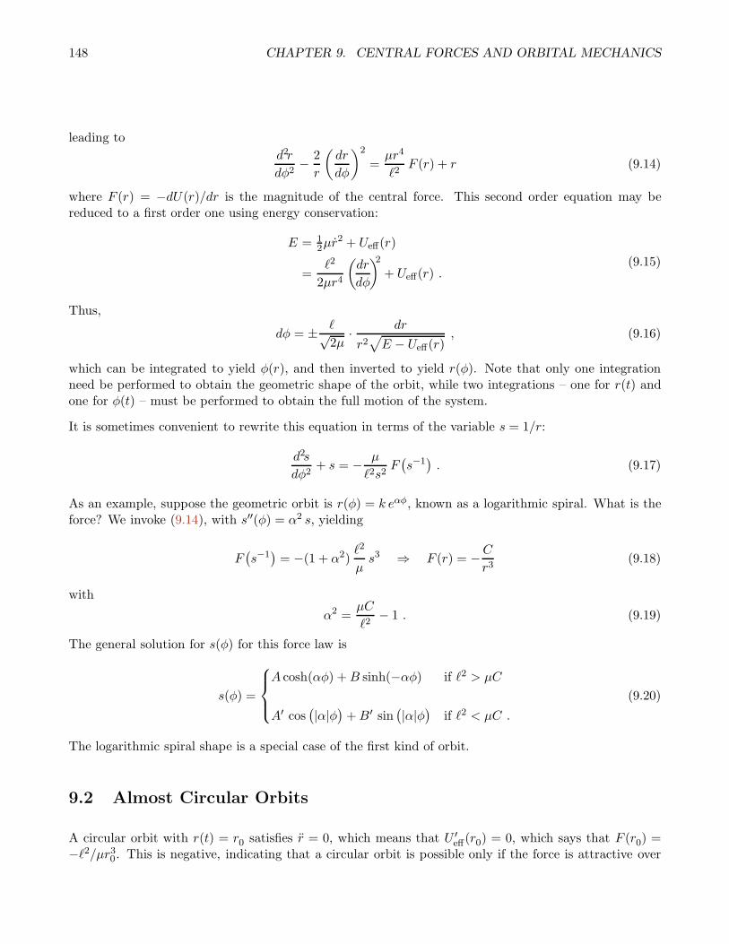
148 CHAPTER 9. CENTRAL FORCES AND ORBITAL MECHANICS
leading to
d2r
dφ2− 2
r
(dr
dφ
)2
=µr4
ℓ2F (r) + r (9.14)
where F (r) = −dU(r)/dr is the magnitude of the central force. This second order equation may bereduced to a first order one using energy conservation:
E = 12µr
2 + Ueff(r)
=ℓ2
2µr4
(dr
dφ
)2+ Ueff(r) .
(9.15)
Thus,
dφ = ± ℓ√2µ
· dr
r2√E − Ueff(r)
, (9.16)
which can be integrated to yield φ(r), and then inverted to yield r(φ). Note that only one integrationneed be performed to obtain the geometric shape of the orbit, while two integrations – one for r(t) andone for φ(t) – must be performed to obtain the full motion of the system.
It is sometimes convenient to rewrite this equation in terms of the variable s = 1/r:
d2s
dφ2+ s = − µ
ℓ2s2F(s−1). (9.17)
As an example, suppose the geometric orbit is r(φ) = k eαφ, known as a logarithmic spiral. What is theforce? We invoke (9.14), with s′′(φ) = α2 s, yielding
F(s−1)= −(1 + α2)
ℓ2
µs3 ⇒ F (r) = −C
r3(9.18)
with
α2 =µC
ℓ2− 1 . (9.19)
The general solution for s(φ) for this force law is
s(φ) =
A cosh(αφ) +B sinh(−αφ) if ℓ2 > µC
A′ cos(|α|φ
)+B′ sin
(|α|φ
)if ℓ2 < µC .
(9.20)
The logarithmic spiral shape is a special case of the first kind of orbit.
9.2 Almost Circular Orbits
A circular orbit with r(t) = r0 satisfies r = 0, which means that U ′eff(r0) = 0, which says that F (r0) =
−ℓ2/µr30. This is negative, indicating that a circular orbit is possible only if the force is attractive over

9.2. ALMOST CIRCULAR ORBITS 149
Figure 9.2: Stable and unstable circular orbits. Left panel: U(r) = −k/r produces a stable circularorbit. Right panel: U(r) = −k/r4 produces an unstable circular orbit.
some range of distances. Since r = 0 as well, we must also have E = Ueff(r0). An almost circular orbithas r(t) = r0 + η(t), where |η/r0| ≪ 1. To lowest order in η, one derives the equations
d2η
dt2= −ω2 η , ω2 =
1
µU ′′eff(r0) . (9.21)
If ω2 > 0, the circular orbit is stable and the perturbation oscillates harmonically. If ω2 < 0, the circularorbit is unstable and the perturbation grows exponentially. For the geometric shape of the perturbedorbit, we write r = r0 + η, and from (9.14) we obtain
d2η
dφ2=
(µr40ℓ2
F ′(r0)− 3
)η = −β2 η , (9.22)
with
β2 = 3 +d lnF (r)
d ln r
∣∣∣∣∣r0
. (9.23)
The solution here isη(φ) = η0 cos β(φ− δ0) , (9.24)
where η0 and δ0 are initial conditions. Setting η = η0, we obtain the sequence of φ values
φn = δ0 +2πn
β, (9.25)
at which η(φ) is a local maximum, i.e. at apoapsis, where r = r0+η0. Setting r = r0−η0 is the conditionfor closest approach, i.e. periapsis. This yields the identical set if angles, just shifted by π. The difference,
∆φ = φn+1 − φn − 2π = 2π(β−1 − 1
), (9.26)
is the amount by which the apsides (i.e. periapsis and apoapsis) precess during each cycle. If β > 1, theapsides advance, i.e. it takes less than a complete revolution ∆φ = 2π between successive periapses. If

150 CHAPTER 9. CENTRAL FORCES AND ORBITAL MECHANICS
β < 1, the apsides retreat, and it takes longer than a complete revolution between successive periapses.The situation is depicted in Fig. 9.3 for the case β = 1.1. Below, we will exhibit a soluble model in whichthe precessing orbit may be determined exactly. Finally, note that if β = p/q is a rational number, thenthe orbit is closed , i.e. it eventually retraces itself, after every q revolutions.
As an example, let F (r) = −kr−α. Solving for a circular orbit, we write
U ′eff(r) =
k
rα− ℓ2
µr3= 0 , (9.27)
which has a solution only for k > 0, corresponding to an attractive potential. We then find
r0 =
(ℓ2
µk
)1/(3−α)
, (9.28)
and β2 = 3− α. The shape of the perturbed orbits follows from η′′ = −β2 η. Thus, while circular orbitsexist whenever k > 0, small perturbations about these orbits are stable only for β2 > 0, i.e. for α < 3.One then has η(φ) = A cos β(φ − φ0). The perturbed orbits are closed, at least to lowest order in η, forα = 3 − (p/q)2, i.e. for β = p/q. The situation is depicted in Fig. 9.2, for the potentials U(r) = −k/r(α = 2) and U(r) = −k/r4 (α = 5).
9.3 Precession in a Soluble Model
Let’s start with the answer and work backwards. Consider the geometrical orbit,
r(φ) =r0
1− ǫ cos βφ. (9.29)
Our interest is in bound orbits, for which 0 ≤ ǫ < 1 (see Fig. 9.3). What sort of potential gives rise tothis orbit? Writing s = 1/r as before, we have
s(φ) = s0 (1− ε cos βφ) . (9.30)
Substituting into (9.17), we have
− µ
ℓ2s2F(s−1)=
d2s
dφ2+ s
= β2 s0 ǫ cos βφ+ s
= (1− β2) s + β2 s0 ,
(9.31)
from which we conclude
F (r) = − k
r2+C
r3, (9.32)
with
k = β2s0ℓ2
µ, C = (β2 − 1)
ℓ2
µ. (9.33)

9.3. PRECESSION IN A SOLUBLE MODEL 151
Figure 9.3: Precession in a soluble model, with geometric orbit r(φ) = r0/(1−ε cos βφ), shown here withβ = 1.1. Periapsis and apoapsis advance by ∆φ = 2π(1 − β−1) per cycle.
The corresponding potential is
U(r) = −kr+
C
2r2+ U∞ , (9.34)
where U∞ is an arbitrary constant, conveniently set to zero. If µ and C are given, we have
r0 =ℓ2
µk+C
k, β =
√1 +
µC
ℓ2. (9.35)
When C = 0, these expressions recapitulate those from the Kepler problem. Note that when ℓ2+µC < 0that the effective potential is monotonically increasing as a function of r. In this case, the angularmomentum barrier is overwhelmed by the (attractive, C < 0) inverse square part of the potential, andUeff(r) is monotonically increasing. The orbit then passes through the force center. It is a useful exerciseto derive the total energy for the orbit,
E = (ε2 − 1)µk2
2(ℓ2 + µC)⇐⇒ ε2 = 1 +
2E(ℓ2 + µC)
µk2. (9.36)

152 CHAPTER 9. CENTRAL FORCES AND ORBITAL MECHANICS
Figure 9.4: The effective potential for the Kepler problem, and associated phase curves. The orbits aregeometrically described as conic sections: hyperbolae (E > 0), parabolae (E = 0), ellipses (Emin < E <0), and circles (E = Emin).
9.4 The Kepler Problem: U(r) = −k r−1
9.4.1 Geometric shape of orbits
The force is F (r) = −kr−2, hence the equation for the geometric shape of the orbit is
d2s
dφ2+ s = − µ
ℓ2s2F (s−1) =
µk
ℓ2, (9.37)
with s = 1/r. Thus, the most general solution is
s(φ) = s0 − C cos(φ− φ0) , (9.38)
where C and φ0 are constants. Thus,
r(φ) =r0
1− ε cos(φ− φ0), (9.39)
where r0 = ℓ2/µk and where we have defined a new constant ε ≡ Cr0.
9.4.2 Laplace-Runge-Lenz vector
Consider the vectorA = p× ℓ− µk r , (9.40)

9.4. THE KEPLER PROBLEM: U(R) = −KR−1 153
where r = r/|r| is the unit vector pointing in the direction of r. We may now show that A is conserved:
dA
dt=
d
dt
p× ℓ− µk
r
r
= p× ℓ+ p× ℓ− µkrr − rrr2
= −krr3
× (µr × r)− µkr
r+ µk
rr
r2
= −µk r(r · r)r3
+ µkr(r · r)r3
− µkr
r+ µk
rr
r2= 0 .
(9.41)
So A is a conserved vector which clearly lies in the plane of the motion. A points toward periapsis, i.e.toward the point of closest approach to the force center.
Let’s assume apoapsis occurs at φ = φ0. Then
A · r = −Ar cos(φ− φ0) = ℓ2 − µkr (9.42)
giving
r(φ) =ℓ2
µk −A cos(φ− φ0)=
a(1− ε2)
1− ε cos(φ− φ0), (9.43)
where
ε =A
µk, a(1− ε2) =
ℓ2
µk. (9.44)
The orbit is a conic section with eccentricity ε. Squaring A, one finds
A2 = (p× ℓ)2 − 2µk r · p× ℓ+ µ2k2
= p2ℓ2 − 2µℓ2k
r+ µ2k2
= 2µℓ2(p2
2µ− k
r+µk2
2ℓ2
)= 2µℓ2
(E +
µk2
2ℓ2
) (9.45)
and thus
a = − k
2E, ε2 = 1 +
2Eℓ2
µk2. (9.46)
9.4.3 Kepler orbits are conic sections
There are four classes of conic sections:
• Circle: ε = 0, E = −µk2/2ℓ2, radius a = ℓ2/µk. The force center lies at the center of circle.
• Ellipse: 0 < ε < 1, −µk2/2ℓ2 < E < 0, semimajor axis a = −k/2E, semiminor axis b = a√1− ε2.
The force center is at one of the foci.
• Parabola: ε = 1, E = 0, force center is the focus.

154 CHAPTER 9. CENTRAL FORCES AND ORBITAL MECHANICS
Figure 9.5: Keplerian orbits are conic sections, classified according to eccentricity: hyperbola (ǫ > 1),parabola (ǫ = 1), ellipse (0 < ǫ < 1), and circle (ǫ = 0). The Laplace-Runge-Lenz vector, A, pointstoward periapsis.
• Hyperbola: ε > 1, E > 0, force center is closest focus (attractive) or farthest focus (repulsive).
To see that the Keplerian orbits are indeed conic sections, consider the ellipse of Fig. 9.6. The law ofcosines gives
ρ2 = r2 + 4f2 − 4rf cosφ , (9.47)
where f = εa is the focal distance. Now for any point on an ellipse, the sum of the distances to the leftand right foci is a constant, and taking φ = 0 we see that this constant is 2a. Thus, ρ = 2a− r, and wehave
(2a− r)2 = 4a2 − 4ar + r2 = r2 + 4ε2a2 − 4εr cosφ
⇒ r(1− ε cosφ) = a(1− ε2) .(9.48)
Thus, we obtain
r(φ) =a (1− ε2)
1− ε cosφ, (9.49)
and we therefore conclude that
r0 =ℓ2
µk= a (1− ε2) . (9.50)

9.4. THE KEPLER PROBLEM: U(R) = −KR−1 155
Figure 9.6: The Keplerian ellipse, with the force center at the left focus. The focal distance is f = εa,where a is the semimajor axis length. The length of the semiminor axis is b =
√1− ε2 a.
Next let us examine the energy,
E = 12µr
2 + Ueff(r)
= 12µ
(ℓ
µr2dr
dφ
)2+
ℓ2
2µr2− k
r
=ℓ2
2µ
(ds
dφ
)2+ℓ2
2µs2 − ks ,
(9.51)
with
s =1
r=µk
ℓ2
(1− ε cos φ
). (9.52)
Thus,ds
dφ=µk
ℓ2ε sinφ , (9.53)
and(ds
dφ
)2=µ2k2
ℓ4ε2 sin2φ
=µ2k2ε2
ℓ4−(µk
ℓ2− s
)2
= −s2 + 2µk
ℓ2s+
µ2k2
ℓ4(ε2 − 1
).
(9.54)
Substituting this into eqn. 9.51, we obtain
E =µk2
2ℓ2(ε2 − 1
). (9.55)
For the hyperbolic orbit, depicted in Fig. 9.7, we have r− ρ = ∓2a, depending on whether we are on theattractive or repulsive branch, respectively. We then have
(r ± 2a)2 = 4a2 ± 4ar + r2 = r2 + 4ε2a2 − 4εr cosφ
⇒ r(±1 + ε cosφ) = a(ε2 − 1) .(9.56)

156 CHAPTER 9. CENTRAL FORCES AND ORBITAL MECHANICS
Figure 9.7: The Keplerian hyperbolae, with the force center at the left focus. The left (blue) branchcorresponds to an attractive potential, while the right (red) branch corresponds to a repulsive potential.The equations of these branches are r = ρ = ∓2a, where the top sign corresponds to the left branch andthe bottom sign to the right branch.
This yields
r(φ) =a (ε2 − 1)
±1 + ε cos φ. (9.57)
9.4.4 Period of bound Kepler orbits
From ℓ = µr2φ = 2µA, the period is τ = 2µA/ℓ, where A = πa2√1− ε2 is the area enclosed by the orbit.
This gives
τ = 2π
(µa3
k
)1/2
= 2π
(a3
GM
)1/2
(9.58)
as well asa3
τ2=GM
4π2, (9.59)
where k = Gm1m2 and M = m1+m2 is the total mass. For planetary orbits, m1 =M⊙ is the solar mass
and m2 = mp is the planetary mass. We then have
a3
τ2=(1 +
mp
M⊙
)GM⊙4π2
≈ GM⊙4π2
, (9.60)
which is to an excellent approximation independent of the planetary mass. (Note that mp/M⊙ ≈ 10−3
even for Jupiter.) This analysis also holds, mutatis mutandis, for the case of satellites orbiting the earth,and indeed in any case where the masses are grossly disproportionate in magnitude.

9.4. THE KEPLER PROBLEM: U(R) = −KR−1 157
9.4.5 Escape velocity
The threshold for escape from a gravitational potential occurs at E = 0. Since E = T + U is conserved,we determine the escape velocity for a body a distance r from the force center by setting
E = 0 = 12µv
2esc(t)−
GMm
r⇒ vesc(r) =
√2G(M +m)
r. (9.61)
When M ≫ m, vesc(r) =√2GM/r. Thus, for an object at the surface of the earth, vesc =
√2gRE =
11.2 km/s.
9.4.6 Satellites and spacecraft
A satellite in a circular orbit a distance h above the earth’s surface has an orbital period
τ =2π√GME
(RE + h)3/2 , (9.62)
where we take msatellite ≪ ME. For low earth orbit (LEO), h ≪ RE = 6.37 × 10⁶ m, in which case
τLEO = 2π√RE/g = 1.4 hr.
Consider a weather satellite in an elliptical orbit whose closest approach to the earth (perigee) is 200km above the earth’s surface and whose farthest distance (apogee) is 7200 km above the earth’s surface.What is the satellite’s orbital period? From Fig. 9.6, we see that
dapogee = RE + 7200 km = 13571 km
dperigee = RE + 200 km = 6971 km
a = 12 (dapogee + dperigee) = 10071 km .
(9.63)
We then have
τ =( a
RE
)3/2· τLEO ≈ 2.65 hr . (9.64)
What happens if a spacecraft in orbit about the earth fires its rockets? Clearly the energy and angularmomentum of the orbit will change, and this means the shape will change. If the rockets are fired (in thedirection of motion) at perigee, then perigee itself is unchanged, because v ·r = 0 is left unchanged at this
point. However, E is increased, hence the eccentricity ε =√
1 + 2Eℓ2
µk2increases. This is the most efficient
way of boosting a satellite into an orbit with higher eccentricity. Conversely, and somewhat paradoxically,when a satellite in LEO loses energy due to frictional drag of the atmosphere, the energy E decreases.Initially, because the drag is weak and the atmosphere is isotropic, the orbit remains circular. Since Edecreases, 〈T 〉 = −E must increase, which means that the frictional forces cause the satellite to speedup!
9.4.7 Two examples of orbital mechanics
• Problem #1: At perigee of an elliptical Keplerian orbit, a satellite receives an impulse ∆p = p0r.Describe the resulting orbit.
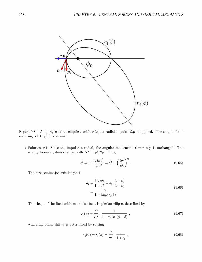
158 CHAPTER 9. CENTRAL FORCES AND ORBITAL MECHANICS
Figure 9.8: At perigee of an elliptical orbit ri(φ), a radial impulse ∆p is applied. The shape of theresulting orbit rf(φ) is shown.
Solution #1: Since the impulse is radial, the angular momentum ℓ = r × p is unchanged. Theenergy, however, does change, with ∆E = p20/2µ. Thus,
ε2f = 1 +2Efℓ
2
µk2= ε2i +
(ℓp0µk
)2
. (9.65)
The new semimajor axis length is
af =ℓ2/µk
1− ε2f= ai ·
1− ε2i1− ε2f
=ai
1− (aip20/µk)
.
(9.66)
The shape of the final orbit must also be a Keplerian ellipse, described by
rf(φ) =ℓ2
µk· 1
1− εf cos(φ+ δ), (9.67)
where the phase shift δ is determined by setting
ri(π) = rf(π) =ℓ2
µk· 1
1 + εi. (9.68)

9.4. THE KEPLER PROBLEM: U(R) = −KR−1 159
Figure 9.9: The larger circular orbit represents the orbit of the earth. The elliptical orbit represents thatfor an object orbiting the Sun with distance at perihelion equal to the Sun’s radius.
Solving for δ, we obtain
δ = cos−1(εi/εf
). (9.69)
The situation is depicted in Fig. 9.8.
• Problem #2: Which is more energy efficient – to send nuclear waste outside the solar system, or tosend it into the Sun?
Solution #2: Escape velocity for the solar system is vesc,⊙(r) =√GM⊙/r. At a distance aE, we
then have vesc,⊙(aE) =√2 vE, where vE =
√GM⊙/aE = 2πaE/τE = 29.9 km/s is the velocity of the
earth in its orbit. The satellite is launched from earth, and clearly the most energy efficient launchwill be one in the direction of the earth’s motion, in which case the velocity after escape from earthmust be u =
(√2 − 1
)vE = 12.4 km/s. The speed just above the earth’s atmosphere must then be
u, where
12mu
2 − GMEm
RE
= 12mu
2 , (9.70)
or, in other words,
u2 = u2 + v2esc,E . (9.71)
We compute u = 16.7 km/s.
The second method is to place the trash ship in an elliptical orbit whose perihelion is the Sun’sradius, R⊙ = 6.98×10⁸ m, and whose aphelion is aE. Using the general equation r(φ) = (ℓ2/µk)/(1−ε cos φ) for a Keplerian ellipse, we therefore solve the two equations
r(φ = π) = R⊙ =1
1 + ε· ℓ
2
µk
r(φ = 0) = aE =1
1− ε· ℓ
2
µk.
(9.72)

160 CHAPTER 9. CENTRAL FORCES AND ORBITAL MECHANICS
We thereby obtain
ε =aE −R⊙aE +R⊙
= 0.991 , (9.73)
which is a very eccentric ellipse, and
ℓ2
µk=
a2E v2
G(M⊙ +m)≈ aE · v
2
v2E
= (1− ε) aE =2aER⊙aE +R⊙
.
(9.74)
Hence,
v2 =2R⊙
aE +R⊙v2E , (9.75)
and the necessary velocity relative to earth is
u =
(√2R⊙
aE +R⊙− 1
)vE ≈ −0.904 vE , (9.76)
i.e. u = −27.0 km/s. Launch is in the opposite direction from the earth’s orbital motion, and fromu2 = u2 + v2esc,E we find u = −29.2 km/s, which is larger (in magnitude) than in the first scenario.Thus, it is cheaper to ship the trash out of the solar system than to send it crashing into the Sun,by a factor u2I /u
2II = 0.327.
9.5 Appendix I : Mission to Neptune
Four earth-launched spacecraft have escaped the solar system: Pioneer 10 (launch 3/3/72), Pioneer 11
(launch 4/6/73), Voyager 1 (launch 9/5/77), and Voyager 2 (launch 8/20/77).1 The latter two are stillfunctioning, and each are moving away from the Sun at a velocity of roughly 3.5 AU/yr.
As the first objects of earthly origin to leave our solar system, both Pioneer spacecraft featured a graphicmessage in the form of a 6” x 9” gold anodized plaque affixed to the spacecrafts’ frame. This plaquewas designed in part by the late astronomer and popular science writer Carl Sagan. The humorist DaveBarry, in an essay entitled Bring Back Carl’s Plaque, remarks,
But the really bad part is what they put on the plaque. I mean, if we’re going to have aplaque, it ought to at least show the aliens what we’re really like, right? Maybe a picture ofpeople eating cheeseburgers and watching “The Dukes of Hazzard.” Then if aliens found it,they’d say, “Ah. Just plain folks.”
But no. Carl came up with this incredible science-fair-wimp plaque that features drawings of– you are not going to believe this – a hydrogen atom and naked people. To represent theentire Earth! This is crazy! Walk the streets of any town on this planet, and the two thingsyou will almost never see are hydrogen atoms and naked people.

9.5. APPENDIX I : MISSION TO NEPTUNE 161
Figure 9.10: The unforgivably dorky Pioneer 10 and Pioneer 11 plaque.
During August, 1989, Voyager 2 investigated the planet Neptune. A direct trip to Neptune along aKeplerian ellipse with rp = aE = 1AU and ra = aN = 30.06AU would take 30.6 years. To see this, note
that rp = a (1− ε) and ra = a (1 + ε) yield
a = 12
(aE + aN
)= 15.53AU , ε =
aN − aE
aN + aE
= 0.9356 . (9.77)
Thus,
τ = 12 τE ·
( aaE
)3/2= 30.6 yr . (9.78)
The energy cost per kilogram of such a mission is computed as follows. Let the speed of the probeafter its escape from earth be vp = λvE, and the speed just above the atmosphere (i.e. neglecting
atmospheric friction) is v0. For the most efficient launch possible, the probe is shot in the direction ofearth’s instantaneous motion about the Sun. Then we must have
12mv20 −
GMEm
RE
= 12m (λ− 1)2 v2E , (9.79)
since the speed of the probe in the frame of the earth is vp − vE = (λ− 1) vE. Thus,
E
m= 1
2v20 =
[12(λ− 1)2 + h
]v2E
v2E =GM⊙aE
= 6.24 × 10⁷ RJ/kg ,(9.80)
1There is a very nice discussion in the Barger and Olsson book on ‘Grand Tours of the Outer Planets’. Here I reconstructand extend their discussion.

162 CHAPTER 9. CENTRAL FORCES AND ORBITAL MECHANICS
Figure 9.11: Mission to Neptune. The figure at the lower right shows the orbits of Earth, Jupiter, andNeptune in black. The cheapest (in terms of energy) direct flight to Neptune, shown in blue, would take30.6 years. By swinging past the planet Jupiter, the satellite can pick up great speed and with evenless energy the mission time can be cut to 8.5 years (red curve). The inset in the upper left shows thescattering event with Jupiter.
where
h ≡ ME
M⊙· aE
RE
= 7.050 × 10⁻² . (9.81)
Therefore, a convenient dimensionless measure of the energy is
η ≡ 2E
mv2E=v20v2E
= (λ− 1)2 + 2h . (9.82)
As we shall derive below, a direct mission to Neptune requires
λ ≥√
2aN
aN + aE
= 1.3913 , (9.83)
which is close to the criterion for escape from the solar system, λesc =√2. Note that about 52% of the
energy is expended after the probe escapes the Earth’s pull, and 48% is expended in liberating the probefrom Earth itself.
This mission can be done much more economically by taking advantage of a Jupiter flyby, as shownin Fig. 9.11. The idea of a flyby is to steal some of Jupiter’s momentum and then fly away very fast

9.5. APPENDIX I : MISSION TO NEPTUNE 163
before Jupiter realizes and gets angry. The CM frame of the probe-Jupiter system is of course the restframe of Jupiter, and in this frame conservation of energy means that the final velocity uf is of the same
magnitude as the initial velocity ui. However, in the frame of the Sun, the initial and final velocities are
vJ + ui and vJ + uf , respectively, where vJ is the velocity of Jupiter in the rest frame of the Sun. If, as
shown in the inset to Fig. 9.11, uf is roughly parallel to vJ, the probe’s velocity in the Sun’s frame willbe enhanced. Thus, the motion of the probe is broken up into three segments:
I : Earth to Jupiter
II : Scatter off Jupiter’s gravitational pull
III : Jupiter to Neptune
We now analyze each of these segments in detail. In so doing, it is useful to recall that the general formof a Keplerian orbit is
r(φ) =d
1− ε cos φ, d =
ℓ2
µk=∣∣ε2 − 1
∣∣ a . (9.84)
The energy is
E = (ε2 − 1)µk2
2ℓ2, (9.85)
with k = GMm, where M is the mass of either the Sun or a planet. In either case, M dominates, andµ =Mm/(M +m) ≃ m to extremely high accuracy. The time for the trajectory to pass from φ = φ1 to
φ = φ2 is
T =
∫dt =
φ2∫
φ1
dφ
φ=µ
ℓ
φ2∫
φ1
dφ r2(φ) =ℓ3
µk2
φ2∫
φ1
dφ[1− ε cosφ
]2 . (9.86)
For reference,
aE = 1AU aJ = 5.20AU aN = 30.06AU
ME = 5.972 × 1024 kg MJ = 1.900 × 1027 kg M⊙ = 1.989 × 1030 kg
with 1AU = 1.496 × 10⁸ km. Here aE,J,N and ME,J,⊙ are the orbital radii and masses of Earth, Jupiter,and Neptune, and the Sun. The last thing we need to know is the radius of Jupiter,
RJ = 9.558 × 10⁻⁴ AU .
We need RJ because the distance of closest approach to Jupiter, or perijove, must be RJ or greater, orelse the probe crashes into Jupiter!
9.5.1 I. Earth to Jupiter
The probe’s velocity at perihelion is vp = λvE. The angular momentum is ℓ = µaE · λvE, whence
d =(aEλvE)
2
GM⊙= λ2 aE . (9.87)

164 CHAPTER 9. CENTRAL FORCES AND ORBITAL MECHANICS
From r(π) = aE, we obtain
εI = λ2 − 1 . (9.88)
This orbit will intersect the orbit of Jupiter if ra ≥ aJ, which means
d
1− εI≥ aJ ⇒ λ ≥
√2aJ
aJ + aE
= 1.2952 . (9.89)
If this inequality holds, then intersection of Jupiter’s orbit will occur for
φJ = 2π − cos−1
(aJ − λ2aE
(λ2 − 1) aJ
). (9.90)
Finally, the time for this portion of the trajectory is
τEJ = τE · λ3φJ∫
π
dφ
2π
1[1− (λ2 − 1) cos φ
]2 . (9.91)
9.5.2 II. Encounter with Jupiter
We are interested in the final speed vf of the probe after its encounter with Jupiter. We will determine
the speed vf and the angle δ which the probe makes with respect to Jupiter after its encounter. Accordingto the geometry of Fig. 9.11,
v2f = v2J + u2 − 2uvJ cos(χ+ γ)
cos δ =v2J + v2f − u2
2vfvJ
(9.92)
Note that
v2J =GM⊙aJ
=aE
aJ
· v2E . (9.93)
But what are u, χ, and γ?
To determine u, we invokeu2 = v2J + v2i − 2vJvi cos β . (9.94)
The initial velocity (in the frame of the Sun) when the probe crosses Jupiter’s orbit is given by energyconservation:
12m(λvE)
2 − GM⊙m
aE
= 12mv
2i −
GM⊙m
aJ
, (9.95)
which yields
v2i =(λ2 − 2 +
2aE
aJ
)v2E . (9.96)
As for β, we invoke conservation of angular momentum:
µ(vi cos β)aJ = µ(λvE)aE ⇒ vi cos β = λaE
aJ
vE . (9.97)

9.5. APPENDIX I : MISSION TO NEPTUNE 165
The angle γ is determined from
vJ = vi cos β + u cos γ . (9.98)
Putting all this together, we obtain
vi = vE√λ2 − 2 + 2x
u = vE√λ2 − 2 + 3x− 2λx3/2
cos γ =
√x− λx√
λ2 − 2 + 3x− 2λx3/2,
(9.99)
where
x ≡ aE
aJ
= 0.1923 . (9.100)
We next consider the scattering of the probe by the planet Jupiter. In the Jovian frame, we may write
r(φ) =κRJ (1 + εJ)
1 + εJ cosφ, (9.101)
where perijove occurs at
r(0) = κRJ . (9.102)
Here, κ is a dimensionless quantity, which is simply perijove in units of the Jovian radius. Clearly werequire κ > 1 or else the probe crashes into Jupiter! The probe’s energy in this frame is simply E = 1
2mu2,
which means the probe enters into a hyperbolic orbit about Jupiter. Next, from
E =k
2
ε2 − 1
ℓ2/µk
ℓ2
µk= (1 + ε)κRJ
(9.103)
we find
εJ = 1 + κ
(RJ
aE
)(M⊙MJ
)(u
vE
)2. (9.104)
The opening angle of the Keplerian hyperbola is then φc = cos−1(ε−1J
), and the angle χ is related to φc
through
χ = π − 2φc = π − 2 cos−1
(1
εJ
). (9.105)
Therefore, we may finally write
vf =
√x v2E + u2 + 2u vE
√x cos(2φc − γ)
cos δ =x v2E + v2f − u2
2 vf vE√x
.(9.106)

166 CHAPTER 9. CENTRAL FORCES AND ORBITAL MECHANICS
Figure 9.12: Total time for Earth-Neptune mission as a function of dimensionless velocity at perihelion,λ = vp/vE. Six different values of κ, the value of perijove in units of the Jovian radius, are shown: κ = 1.0(thick blue), κ = 5.0 (red), κ = 20 (green), κ = 50 (blue), κ = 100 (magenta), and κ = ∞ (thick black).
9.5.3 III. Jupiter to Neptune
Immediately after undergoing gravitational scattering off Jupiter, the energy and angular momentum ofthe probe are
E = 12mv
2f −
GM⊙m
aJ
(9.107)
and
ℓ = µ vf aJ cos δ . (9.108)
We write the geometric equation for the probe’s orbit as
r(φ) =d
1 + ε cos(φ− φJ − α), (9.109)
where
d =ℓ2
µk=
(vf aJ cos δ
vE aE
)2aE . (9.110)
Setting E = (µk2/2ℓ2)(ε2 − 1), we obtain the eccentricity
ε =
√√√√1 +
(v2fv2E
− 2aE
aJ
)d
aE
. (9.111)

9.6. APPENDIX II : RESTRICTED THREE-BODY PROBLEM 167
Note that the orbit is hyperbolic – the probe will escape the Sun – if vf > vE ·√2x. The condition that
this orbit intersect Jupiter at φ = φJ yields
cosα =1
ε
(d
aJ
− 1
), (9.112)
which determines the angle α. Interception of Neptune occurs at
d
1 + ε cos(φN − φJ − α)= aN ⇒ φN = φJ + α+ cos−1 1
ε
(d
aN
− 1
). (9.113)
We then have
τJN = τE ·(d
aE
)3 φN∫
φJ
dφ
2π
1[1 + ε cos(φ− φJ − α)
]2 . (9.114)
The total time to Neptune is then the sum,
τEN = τEJ + τJN . (9.115)
In Fig. 9.12, we plot the mission time τEN versus the velocity at perihelion, vp = λvE, for various valuesof κ. The value κ = ∞ corresponds to the case of no Jovian encounter at all.
9.6 Appendix II : Restricted Three-Body Problem
Problem : Consider the ‘restricted three body problem’ in which a light object of mass m (e.g. a satellite)moves in the presence of two celestial bodies of masses m1 and m2 (e.g. the sun and the earth, or theearth and the moon). Suppose m1 and m2 execute stable circular motion about their common center ofmass. You may assume m≪ m2 ≤ m1.
(a) Show that the angular frequency for the motion of masses 1 and 2 is related to their (constant)relative separation, by
ω20 =
GM
r30, (9.116)
where M = m1 +m2 is the total mass.
Solution : For a Kepler potential U = −k/r, the circular orbit lies at r0 = ℓ2/µk, where ℓ = µr2φ is theangular momentum and k = Gm1m2. This gives
ω20 =
ℓ2
µ2 r40=
k
µr30=GM
r30, (9.117)
with ω0 = φ.
(b) The satellite moves in the combined gravitational field of the two large bodies; the satellite itself isof course much too small to affect their motion. In deriving the motion for the satellilte, it is convenient

168 CHAPTER 9. CENTRAL FORCES AND ORBITAL MECHANICS
Figure 9.13: The Lagrange points for the earth-sun system. Credit: WMAP project.
to choose a reference frame whose origin is the CM and which rotates with angular velocity ω0. In the
rotating frame the masses m1 and m2 lie, respectively, at x1 = −αr0 and x2 = βr0, with
α =m2
M, β =
m1
M(9.118)
and with y1 = y2 = 0. Note α+ β = 1.
Show that the Lagrangian for the satellite in this rotating frame may be written
L = 12m(x− ω0 y
)2+ 1
2m(y + ω0 x
)2+
Gm1m√(x+ αr0)
2 + y2+
Gm2m√(x− βr0)
2 + y2. (9.119)
Solution : Let the original (inertial) coordinates be (x0, y0). Then let us define the rotated coordinates(x, y) as
x = cos(ω0t)x0 + sin(ω0t) y0
y = − sin(ω0t)x0 + cos(ω0t) y0 .(9.120)
Therefore,
x = cos(ω0t) x0 + sin(ω0t) y0 + ω0 y
y = − sin(ω0t)x0 + cos(ω0t) y0 − ω0 x .(9.121)
Therefore(x− ω0 y)
2 + (y + ω0 x)2 = x20 + y20 , (9.122)

9.6. APPENDIX II : RESTRICTED THREE-BODY PROBLEM 169
The Lagrangian is then
L = 12m(x− ω0 y
)2+ 1
2m(y + ω0 x
)2+
Gm1m√(x− x1)
2 + y2+
Gm2m√(x− x2)
2 + y2, (9.123)
which, with x1 ≡ −αr0 and x2 ≡ βr0, agrees with eqn. 9.119
(c) Lagrange discovered that there are five special points where the satellite remains fixed in the rotatingframe. These are called the Lagrange points L1, L2, L3, L4, L5. A sketch of the Lagrange points forthe earth-sun system is provided in Fig. 9.13. Observation: In working out the rest of this problem, Ifound it convenient to measure all distances in units of r0 and times in units of ω−1
0 , and to eliminate Gby writing Gm1 = β ω2
0 r30 and Gm2 = αω2
0 r30.
Assuming the satellite is stationary in the rotating frame, derive the equations for the positions of theLagrange points.
Solution : At this stage it is convenient to measure all distances in units of r0 and times in units of ω−10
to factor out a term mr20 ω20 from L, writing the dimensionless Lagrangian L ≡ L/(mr20 ω
20). Using as
well the definition of ω20 to eliminate G, we have
L = 12 (ξ − η)2 + 1
2 (η + ξ)2 +β√
(ξ + α)2 + η2+
α√(ξ − β)2 + η2
, (9.124)
with
ξ ≡ x
r0, η ≡ y
r0, ξ ≡ 1
ω0 r0
dx
dt, η ≡ 1
ω0 r0
dy
dt. (9.125)
The equations of motion are then
ξ − 2η = ξ − β(ξ + α)
d31− α(ξ − β)
d32
η + 2ξ = η − βη
d31− αη
d32,
(9.126)
where
d1 =√
(ξ + α)2 + η2 , d2 =√
(ξ − β)2 + η2 . (9.127)
Here, ξ ≡ x/r0, ξ = y/r0, etc. Recall that α+β = 1. Setting the time derivatives to zero yields the staticequations for the Lagrange points:
ξ =β(ξ + α)
d31+α(ξ − β)
d32
η =βη
d31+αη
d32,
(9.128)
(d) Show that the Lagrange points with y = 0 are determined by a single nonlinear equation. Showgraphically that this equation always has three solutions, one with x < x1, a second with x1 < x < x2,and a third with x > x2. These solutions correspond to the points L3, L1, and L2, respectively.

170 CHAPTER 9. CENTRAL FORCES AND ORBITAL MECHANICS
Figure 9.14: Graphical solution for the Lagrange points L1, L2, and L3.
Solution : If η = 0 the second equation is automatically satisfied. The first equation then gives
ξ = β · ξ + α∣∣ξ + α
∣∣3 + α · ξ − β∣∣ξ − β
∣∣3 . (9.129)
The RHS of the above equation diverges to +∞ for ξ = −α+ 0+ and ξ = β + 0+, and diverges to −∞for ξ = −α− 0+ and ξ = β − 0+, where 0+ is a positive infinitesimal. The situation is depicted in Fig.9.14. Clearly there are three solutions, one with ξ < −α, one with −α < ξ < β, and one with ξ > β.
(e) Show that the remaining two Lagrange points, L4 and L5, lie along equilateral triangles with the twomasses at the other vertices.
Solution : If η 6= 0, then dividing the second equation by η yields
1 =β
d31+α
d32. (9.130)
Substituting this into the first equation,
ξ =
(β
d31+α
d32
)ξ +
(1
d31− 1
d32
)αβ , (9.131)
givesd1 = d2 . (9.132)

9.6. APPENDIX II : RESTRICTED THREE-BODY PROBLEM 171
Reinserting this into the previous equation then gives the remarkable result,
d1 = d2 = 1 , (9.133)
which says that each of L4 and L5 lies on an equilateral triangle whose two other vertices are the massesm1 and m2. The side length of this equilateral triangle is r0. Thus, the dimensionless coordinates of L4and L5 are (
ξL4, ηL4
)=(12 − α,
√32
),
(ξL5, ηL5
)=(12 − α, −
√32
). (9.134)
It turns out that L1, L2, and L3 are always unstable. Satellites placed in these positions must undergo pe-riodic course corrections in order to remain approximately fixed. The SOlar and Heliopheric Observationsatellite, SOHO, is located at L1, which affords a continuous unobstructed view of the Sun.
(f) Show that the Lagrange points L4 and L5 are stable (obviously you need only consider one of them)provided that the mass ratio m1/m2 is sufficiently large. Determine this critical ratio. Also find thefrequency of small oscillations for motion in the vicinity of L4 and L5.
Solution : Now we writeξ = ξL4 + δξ , η = ηL4 + δη , (9.135)
and derive the linearized dynamics. Expanding the equations of motion to lowest order in δξ and δη, wehave
δξ − 2δη =
(1− β + 3
2β∂d1∂ξ
∣∣∣∣L4
− α− 32α
∂d2∂ξ
∣∣∣∣L4
)δξ +
(32β
∂d1∂η
∣∣∣∣L4
− 32α
∂d2∂η
∣∣∣∣L4
)δη
= 34 δξ +
3√3
4 ε δη
(9.136)
and
δη + 2δξ =
(3√3
2 β∂d1∂ξ
∣∣∣∣L4
+ 3√3
2 α∂d2∂ξ
∣∣∣∣L4
)δξ +
(3√3
2 β∂d1∂η
∣∣∣∣L4
+ 3√3
2 α∂d2∂η
∣∣∣∣L4
)δη
= 3√3
4 ε δξ + 94 δη ,
(9.137)
where we have defined
ε ≡ β − α =m1 −m2
m1 +m2. (9.138)
As defined, ε ∈ [0, 1].
Fourier transforming the differential equation, we replace each time derivative by (−iν), and therebyobtain (
ν2 + 34 −2iν + 3
4
√3 ε
2iν + 34
√3 ε ν2 + 9
4
)(δξδη
)= 0 . (9.139)
Nontrivial solutions exist only when the determinant D vanishes. One easily finds
D(ν2) = ν4 − ν2 + 2716
(1− ε2
), (9.140)
which yields a quadratic equation in ν2, with roots
ν2 = 12 ± 1
4
√27 ε2 − 23 . (9.141)

172 CHAPTER 9. CENTRAL FORCES AND ORBITAL MECHANICS
These frequencies are dimensionless. To convert to dimensionful units, we simply multiply the solutionsfor ν by ω0, since we have rescaled time by ω−1
0 .
Note that the L4 and L5 points are stable only if ε2 > 2327 . If we define the mass ratio γ ≡ m1/m2, the
stability condition is equivalent to
γ =m1
m2>
√27 +
√23√
27−√23
= 24.960 , (9.142)
which is satisfied for both the Sun-Jupiter system (γ = 1047) – and hence for the Sun and any planet –and also for the Earth-Moon system (γ = 81.2).
Objects found at the L4 and L5 points are called Trojans, after the three large asteroids Agamemnon,Achilles, and Hector found orbiting in the L4 and L5 points of the Sun-Jupiter system. No large asteroidshave been found in the L4 and L5 points of the Sun-Earth system.
Personal aside : David T. Wilkinson
The image in fig. 9.13 comes from the education and outreach program of the Wilkinson MicrowaveAnisotropy Probe (WMAP) project, a NASA mission, launched in 2001, which has produced some ofthe most important recent data in cosmology. The project is named in honor of David T. Wilkinson,who was a leading cosmologist at Princeton, and a founder of the Cosmic Background Explorer (COBE)satellite (launched in 1989). WMAP was sent to the L2 Lagrange point, on the night side of the earth,where it can constantly scan the cosmos with an ultra-sensitive microwave detector, shielded by the earthfrom interfering solar electromagnetic radiation. The L2 point is of course unstable, with a time scale ofabout 23 days. Satellites located at such points must undergo regular course and attitude corrections toremain situated.
During the summer of 1981, as an undergraduate at Princeton, I was a member of Wilkinson’s “gravitygroup,” working under Jeff Kuhn and Ken Libbrecht. It was a pretty big group and Dave – everyonewould call him Dave – used to throw wonderful parties at his home, where we’d always play volleyball.I was very fortunate to get to know David Wilkinson a bit – after working in his group that summer Itook a class from him the following year. He was a wonderful person, a superb teacher, and a world classphysicist.

Chapter 10
Small Oscillations
10.1 Coupled Coordinates
We assume, for a set of n generalized coordinates q1, . . . , qn, that the kinetic energy is a quadraticfunction of the velocities,
T = 12 Tσσ′(q1, . . . , qn) qσ qσ′ , (10.1)
where the sum on σ and σ′ from 1 to n is implied. For example, expressed in terms of polar coordinates(r, θ, φ), the matrix Tij is
Tσσ′ = m
1 0 00 r2 00 0 r2 sin2θ
=⇒ T = 1
2 m(r2 + r2θ2 + r2 sin2θ φ2
). (10.2)
The potential U(q1, . . . , qn) is assumed to be a function of the generalized coordinates alone: U = U(q).A more general formulation of the problem of small oscillations is given in the appendix, section 10.8.
The generalized momenta are
pσ =∂L
∂qσ= Tσσ′ qσ′ , (10.3)
and the generalized forces are
Fσ =∂L
∂qσ=
1
2
∂Tσ′σ′′
∂qσqσ′ qσ′′ −
∂U
∂qσ. (10.4)
The Euler-Lagrange equations are then pσ = Fσ, or
Tσσ′ qσ′ +
(∂Tσσ′
∂qσ′′
− 1
2
∂Tσ′σ′′
∂qσ
)qσ′ qσ′′ = − ∂U
∂qσ(10.5)
which is a set of coupled nonlinear second order ODEs. Here we are using the Einstein ‘summationconvention’, where we automatically sum over any and all repeated indices.
173

174 CHAPTER 10. SMALL OSCILLATIONS
10.2 Expansion about Static Equilibrium
Small oscillation theory begins with the identification of a static equilibrium q1, . . . , qn, which satisfiesthe n nonlinear equations
∂U
∂qσ
∣∣∣∣q=q
= 0 . (10.6)
Once an equilibrium is found (note that there may be more than one static equilibrium), we expandabout this equilibrium, writing
qσ ≡ qσ + ησ . (10.7)
The coordinates η1, . . . , ηn represent the displacements relative to equilibrium.
We next expand the Lagrangian to quadratic order in the generalized displacements, yielding
L = 12Tσσ′ ησ ησ′ − 1
2Vσσ′ ησησ′ , (10.8)
where
Tσσ′ =∂2T
∂qσ ∂qσ′
∣∣∣∣∣q=q
, Vσσ′ =∂2U
∂qσ ∂qσ′
∣∣∣∣∣q=q
. (10.9)
Writing ηt for the row-vector (η1, . . . , ηn), we may suppress indices and write
L = 12 η
tT η − 12 η
tV η , (10.10)
where T and V are the constant matrices of eqn. 10.9.
10.3 Method of Small Oscillations
The idea behind the method of small oscillations is to effect a coordinate transformation from the gen-eralized displacements η to a new set of coordinates ξ, which render the Lagrangian particularly simple.All that is required is a linear transformation,
ησ = Aσi ξi , (10.11)
where both σ and i run from 1 to n. The n × n matrix Aσi is known as the modal matrix. With the
substitution η = A ξ (hence ηt = ξtAt, where Atiσ = Aσi is the matrix transpose), we have
L = 12 ξ
tAtTA ξ − 12 ξ
tAt VA ξ . (10.12)
We now choose the matrix A such that
At TA = I
AtVA = diag(ω21 , . . . , ω
2n
).
(10.13)
With this choice of A, the Lagrangian decouples:
L = 12
n∑
i=1
(ξ2i − ω2
i ξ2i
), (10.14)

10.3. METHOD OF SMALL OSCILLATIONS 175
with the solutionξi(t) = Ci cos(ωi t) +Di sin(ωi t) , (10.15)
where C1, . . . , Cn and D1, . . . ,Dn are 2n constants of integration, and where no sum is implied on i.Note that
ξ = A−1η = AtTη . (10.16)
In terms of the original generalized displacements, the solution is
ησ(t) =
n∑
i=1
Aσi
Ci cos(ωit) +Di sin(ωit)
, (10.17)
and the constants of integration are linearly related to the initial generalized displacements and generalizedvelocities:
Ci = Atiσ Tσσ′ ησ′(0)
Di = ω−1i At
iσ Tσσ′ ησ′(0) ,(10.18)
again with no implied sum on i on the RHS of the second equation, and where we have used A−1 = AtT,from eqns. ??. (The implied sums in eqn. 10.18 are over σ and σ′.)
Note that the normal coordinates have unusual dimensions: [ξ] =√M · L, where L is length and M is
mass.
10.3.1 Can you really just choose an A so that this works?
Yes.
10.3.2 Er...care to elaborate?
Both T and V are symmetric matrices. Aside from that, there is no special relation between them. Inparticular, they need not commute, hence they do not necessarily share any eigenvectors. Nevertheless,they may be simultaneously diagonalized as per ??. Here’s why:
• Since T is symmetric, it can be diagonalized by an orthogonal transformation. That is, there existsa matrix O1 ∈ O(n) such that
Ot1 TO1 = Td , (10.19)
where Td is diagonal.
• We may safely assume that T is positive definite. Otherwise the kinetic energy can become arbitrar-
ily negative, which is unphysical. Therefore, one may form the matrix T−1/2d which is the diagonal
matrix whose entries are the inverse square roots of the corresponding entries of Td. Consider the
linear transformation O1 T−1/2d . Its effect on T is
T−1/2d Ot
1 TO1T−1/2d = 1 . (10.20)

176 CHAPTER 10. SMALL OSCILLATIONS
• Since O1 and Td are wholly derived from T, the only thing we know about
V ≡ T−1/2d Ot
1 VO1 T−1/2d (10.21)
is that it is explicitly a symmetric matrix. Therefore, it may be diagonalized by some orthogonalmatrix O2 ∈ O(n). As T has already been transformed to the identity, the additional orthogonal
transformation has no effect there. Thus, we have shown that there exist orthogonal matrices O1
and O2 such that
Ot2 T
−1/2d Ot
1 TO1 T−1/2d O2 = 1
Ot2 T
−1/2d Ot
1 VO1 T−1/2d O2 = diag (ω2
1, . . . , ω2n) .
(10.22)
All that remains is to identify the modal matrix A = O1 T−1/2d O2.
Note that it is not possible to simultaneously diagonalize three symmetric matrices in general.
10.3.3 Finding the modal matrix
While the above proof allows one to construct A by finding the two orthogonal matrices O1 and O2, sucha procedure is extremely cumbersome. It would be much more convenient if A could be determined inone fell swoop. Fortunately, this is possible.
We start with the equations of motion, T η +V η = 0. In component notation, we have
Tσσ′ ησ′ +Vσσ′ ησ′ = 0 . (10.23)
We now assume that η(t) oscillates with a single frequency ω, i.e. ησ(t) = ψσ e−iωt. This results in a set
of linear algebraic equations for the components ψσ:
(ω2 Tσσ′ −Vσσ′
)ψσ′ = 0 . (10.24)
These are n equations in n unknowns: one for each value of σ = 1, . . . , n. Because the equations arehomogeneous and linear, there is always a trivial solution ψ = 0. In fact one might think this is the onlysolution, since
(ω2T−V
)ψ = 0
?=⇒ ψ =
(ω2 T−V
)−10 = 0 . (10.25)
However, this fails when the matrix ω2 T−V is defective1, i.e. when
det(ω2T−V
)= 0 . (10.26)
Since T and V are of rank n, the above determinant yields an nth order polynomial in ω2, whose n rootsare the desired squared eigenfrequencies ω2
1 , . . . , ω2n.
1The label defective has a distastefully negative connotation. In modern parlance, we should instead refer to such a matrixas determinantally challenged .

10.4. EXAMPLE: MASSES AND SPRINGS 177
Once the n eigenfrequencies are obtained, the modal matrix is constructed as follows. Solve the equations
n∑
σ′=1
(ω2i Tσσ′ −Vσσ′
)ψ(i)σ′ = 0 (10.27)
which are a set of (n − 1) linearly independent equations among the n components of the eigenvectorψ(i). That is, there are n equations (σ = 1, . . . , n), but one linear dependency since det (ω2
i T − V) = 0.The eigenvectors may be chosen to satisfy a generalized orthogonality relationship,
ψ(i)σ Tσσ′ ψ
(j)σ′ = δij . (10.28)
To see this, let us duplicate eqn. 10.27, replacing i with j, and multiply both equations as follows:
ψ(j)σ ×
(ω2i Tσσ′ −Vσσ′
)ψ(i)σ′ = 0
ψ(i)σ ×
(ω2j Tσσ′ −Vσσ′
)ψ(j)σ′ = 0 .
(10.29)
Using the symmetry of T and V, upon subtracting these equations we obtain
(ω2i − ω2
j )n∑
σ,σ′=1
ψ(i)σ Tσσ′ ψ
(j)σ′ = 0 , (10.30)
where the sums on i and j have been made explicit. This establishes that eigenvectors ψ(i) and ψ(j)
corresponding to distinct eigenvalues ω2i 6= ω2
j are orthogonal: (ψ(i))tTψ(j) = 0. For degenerate eigen-values, the eigenvectors are not a priori orthogonal, but they may be orthogonalized via application ofthe Gram-Schmidt procedure. The remaining degrees of freedom - one for each eigenvector – are fixedby imposing the condition of normalization:
ψ(i)σ → ψ(i)
σ
/√ψ(i)µ Tµµ′ ψ
(i)µ′ =⇒ ψ(i)
σ Tσσ′ ψ(j)σ′ = δij . (10.31)
The modal matrix is just the matrix of eigenvectors: Aσi = ψ(i)σ .
With the eigenvectors ψ(i)σ thusly normalized, we have
0 = ψ(i)σ
(ω2j Tσσ′ −Vσσ′
)ψ(j)σ′
= ω2j δij − ψ(i)
σ Vσσ′ ψ(j)σ′ ,
(10.32)
with no sum on j. This establishes the result
AtVA = diag(ω21 , . . . , ω
2n
). (10.33)
10.4 Example: Masses and Springs
Two blocks and three springs are configured as in Fig. 10.1. All motion is horizontal. When the blocksare at rest, all springs are unstretched.

178 CHAPTER 10. SMALL OSCILLATIONS
Figure 10.1: A system of masses and springs.
(a) Choose as generalized coordinates the displacement of each block from its equilibrium position, andwrite the Lagrangian.
(b) Find the T and V matrices.
(c) Suppose
m1 = 2m , m2 = m , k1 = 4k , k2 = k , k3 = 2k ,
Find the frequencies of small oscillations.
(d) Find the normal modes of oscillation.
(e) At time t = 0, mass #1 is displaced by a distance b relative to its equilibrium position. I.e.
x1(0) = b. The other initial conditions are x2(0) = 0, x1(0) = 0, and x2(0) = 0. Find t∗, the next
time at which x2 vanishes.
Solution
(a) The Lagrangian is
L = 12m1 x
21 +
12m2 x
22 − 1
2k1 x21 − 1
2k2 (x2 − x1)2 − 1
2k3 x22
(b) The T and V matrices are
Tij =∂2T
∂xi ∂xj=
(m1 0
0 m2
), Vij =
∂2U
∂xi ∂xj=
(k1 + k2 −k2−k2 k2 + k3
)
(c) We have m1 = 2m, m2 = m, k1 = 4k, k2 = k, and k3 = 2k. Let us write ω2 ≡ λω20, where
ω0 ≡√k/m. Then
ω2T−V = k
(2λ− 5 1
1 λ− 3
).

10.4. EXAMPLE: MASSES AND SPRINGS 179
The determinant is
det (ω2T−V) = (2λ2 − 11λ + 14) k2
= (2λ− 7) (λ − 2) k2 .
There are two roots: λ− = 2 and λ+ = 72 , corresponding to the eigenfrequencies
ω− =
√2k
m, ω+ =
√7k
2m
(d) The normal modes are determined from (ω2aT−V) ~ψ(a) = 0. Plugging in λ = 2 we have for the normal
mode ~ψ(−)
(−1 11 −1
)(ψ(−)
1
ψ(−)
2
)= 0 ⇒ ~ψ(−) = C−
(11
)
Plugging in λ = 72 we have for the normal mode ~ψ(+)
(2 11 1
2
)(ψ(+)
1
ψ(+)
2
)= 0 ⇒ ~ψ(+) = C+
(1−2
)
The standard normalization ψ(a)i Tij ψ
(b)j = δab gives
C− =1√3m
, C+ =1√6m
. (10.34)
(e) The general solution is(x1x2
)= A
(11
)cos(ω−t) +B
(1−2
)cos(ω+t) + C
(11
)sin(ω−t) +D
(1−2
)sin(ω+t) .
The initial conditions x1(0) = b, x2(0) = x1(0) = x2(0) = 0 yield
A = 23b , B = 1
3b , C = 0 , D = 0 .
Thus,
x1(t) =13b ·
(2 cos(ω−t) + cos(ω+t)
)
x2(t) =23b ·
(cos(ω−t)− cos(ω+t)
).
Setting x2(t∗) = 0, we find
cos(ω−t∗) = cos(ω+t
∗) ⇒ π − ω−t = ω+t− π ⇒ t∗ =2π
ω− + ω+

180 CHAPTER 10. SMALL OSCILLATIONS
Figure 10.2: The double pendulum.
10.5 Example: Double Pendulum
As a second example, consider the double pendulum, with m1 = m2 = m and ℓ1 = ℓ2 = ℓ. The kineticand potential energies are
T = mℓ2θ21 +mℓ2 cos(θ1 − θ1) θ1θ2 +12mℓ
2θ22
V = −2mgℓ cos θ1 −mgℓ cos θ2 ,(10.35)
leading to
T =
(2mℓ2 mℓ2
mℓ2 mℓ2
), V =
(2mgℓ 00 mgℓ
). (10.36)
Then
ω2T−V = mℓ2(2ω2 − 2ω2
0 ω2
ω2 ω2 − ω20
), (10.37)
with ω0 =√g/ℓ. Setting the determinant to zero gives
2(ω2 − ω20)
2 − ω4 = 0 ⇒ ω2 = (2±√2)ω2
0 . (10.38)
We find the unnormalized eigenvectors by setting (ω2i T− V )ψ(i) = 0. This gives
ψ+ = C+
(1
−√2
), ψ− = C−
(1
+√2
), (10.39)
where C± are constants. One can check Tσσ′ ψ(i)σ ψ
(j)σ′ vanishes for i 6= j. We then normalize by demanding
Tσσ′ ψ(i)σ ψ
(i)σ′ = 1 (no sum on i), which determines the coefficients C± = 1
2
√(2±
√2)/mℓ2. Thus, the

10.6. ZERO MODES 181
modal matrix is
A =
ψ+1 ψ−
1
ψ+2 ψ−
2
=
1
2√mℓ2
√2 +
√2
√2−
√2
−√4 + 2
√2 +
√4− 2
√2
. (10.40)
10.6 Zero Modes
Recall Noether’s theorem, which says that for every continuous one-parameter family of coordinate trans-formations,
qσ −→ qσ(q, ζ) , qσ(q, ζ = 0) = qσ , (10.41)
which leaves the Lagrangian invariant, i.e. dL/dζ = 0, there is an associated conserved quantity,
Λ =∑
σ
∂L
∂qσ
∂qσ∂ζ
∣∣∣∣∣ζ=0
satisfiesdΛ
dt= 0 . (10.42)
For small oscillations, we write qσ = qσ + ησ, hence
Λk =∑
σ
Ckσ ησ , (10.43)
where k labels the one-parameter families (in the event there is more than one continuous symmetry),and where
Ckσ =∑
σ′
Tσσ′
∂qσ′
∂ζk
∣∣∣∣∣ζ=0
. (10.44)
Therefore, we can define the (unnormalized) normal mode
ξk =∑
σ
Ckσ ησ , (10.45)
which satisfies ξk = 0. Thus, in systems with continuous symmetries, to each such continuous symmetrythere is an associated zero mode of the small oscillations problem, i.e. a mode with ω2
k = 0.
10.6.1 Example of zero mode oscillations
The simplest example of a zero mode would be a pair of masses m1 and m2 moving frictionlessly alonga line and connected by a spring of force constant k. We know from our study of central forces that theLagrangian may be written
L = 12m1x
21 +
12m2x
22 − 1
2k(x1 − x2)2
= 12MX2 + 1
2µx2 − 1
2kx2 ,
(10.46)
where X = (m1x1+m2x2)/(m1+m2) is the center of mass position, x = x1−x2 is the relative coordinate,M = m1 +m2 is the total mass, and µ = m1m2/(m1 +m2) is the reduced mass. The relative coordinate
182 CHAPTER 10. SMALL OSCILLATIONS
Figure 10.3: Coupled oscillations of three masses on a frictionless hoop of radius R. All three springshave the same force constant k, but the masses are all distinct.
obeys x = −ω20 x, where the oscillation frequency is ω0 =
√k/µ. The center of mass coordinate obeys
X = 0, i.e. its oscillation frequency is zero. The center of mass motion is a zero mode.
Another example is furnished by the system depicted in fig. 10.3, where three distinct masses m1, m2,
and m3 move around a frictionless hoop of radius R. The masses are connected to their neighbors by
identical springs of force constant k. We choose as generalized coordinates the angles φσ (σ = 1, 2, 3),with the convention that
φ1 ≤ φ2 ≤ φ3 ≤ 2π + φ1 . (10.47)
Let Rχ be the equilibrium length for each of the springs. Then the potential energy is
U = 12kR
2(φ2 − φ1 − χ)2 + (φ3 − φ2 − χ)2 + (2π + φ1 − φ3 − χ)2
= 12kR
2(φ2 − φ1)
2 + (φ3 − φ2)2 + (2π + φ1 − φ3)
2 + 3χ2 − 4πχ.
(10.48)
Note that the equilibrium angle χ enters only in an additive constant to the potential energy. Thus,for the calculation of the equations of motion, it is irrelevant. It doesn’t matter whether or not theequilibrium configuration is unstretched (χ = 2π/3) or not (χ 6= 2π/3).
The kinetic energy is simple:
T = 12R
2(m1 φ
21 +m2 φ
22 +m3 φ
23
). (10.49)
The T and V matrices are then
T =
m1R
2 0 0
0 m2R2 0
0 0 m3R2
, V =
2kR2 −kR2 −kR2
−kR2 2kR2 −kR2
−kR2 −kR2 2kR2
. (10.50)

10.6. ZERO MODES 183
We then have
ω2T−V = kR2
ω2
Ω21− 2 1 1
1 ω2
Ω22− 2 1
1 1 ω2
Ω23− 2
. (10.51)
We compute the determinant to find the characteristic polynomial:
P (ω) = det(ω2 T−V)
=ω6
Ω21 Ω
22 Ω
23
− 2
(1
Ω21 Ω
22
+1
Ω22 Ω
23
+1
Ω21 Ω
23
)ω4 + 3
(1
Ω21
+1
Ω22
+1
Ω23
)ω2 ,
(10.52)
where Ω2i ≡ k/mi. The equation P (ω) = 0 yields a cubic equation in ω2, but clearly ω2 is a factor, and
when we divide this out we obtain a quadratic equation. One root obviously is ω21 = 0. The other two
roots are solutions to the quadratic equation:
ω22,3 = Ω2
1 +Ω22 +Ω2
3 ±√
12
(Ω2
1 −Ω22
)2+ 1
2
(Ω2
2 −Ω23
)2+ 1
2
(Ω2
1 −Ω23
)2. (10.53)
To find the eigenvectors and the modal matrix, we set
ω2j
Ω21− 2 1 1
1ω2j
Ω22− 2 1
1 1ω2j
Ω23− 2
ψ(j)1
ψ(j)2
ψ(j)3
= 0 , (10.54)
Writing down the three coupled equations for the components of ψ(j), we find
(ω2j
Ω21
− 3
)ψ(j)1 =
(ω2j
Ω22
− 3
)ψ(j)2 =
(ω2j
Ω23
− 3
)ψ(j)3 . (10.55)
We therefore conclude
ψ(j) = Cj
(ω2j
Ω21− 3)−1
(ω2j
Ω22− 3)−1
(ω2j
Ω23− 3)−1
. (10.56)
The normalization condition ψ(i)σ Tσσ′ ψ
(j)σ′ = δij then fixes the constants Cj:
[m1
(ω2j
Ω21
− 3
)−2
+ m2
(ω2j
Ω22
− 3
)−2
+ m3
(ω2j
Ω23
− 3
)−2]∣∣Cj∣∣2 = 1 . (10.57)
The Lagrangian is invariant under the one-parameter family of transformations
φσ −→ φσ + ζ (10.58)

184 CHAPTER 10. SMALL OSCILLATIONS
for all σ = 1, 2, 3. The associated conserved quantity is
Λ =∑
σ
∂L
∂φσ
∂φσ∂ζ
= R2(m1 φ1 +m2 φ2 +m3 φ3
),
(10.59)
which is, of course, the total angular momentum relative to the center of the ring. Thus, from Λ = 0 weidentify the zero mode as ξ1, where
ξ1 = C(m1φ 1 +m2 φ2 +m3φ 3
), (10.60)
where C is a constant. Recall the relation ησ = Aσi ξi between the generalized displacements ησ and the
normal coordinates ξi. We can invert this relation to obtain
ξi = A−1iσ ησ = At
iσ Tσσ′ ησ′ . (10.61)
Here we have used the result AtTA = 1 to write
A−1 = AtT . (10.62)
This is a convenient result, because it means that if we ever need to express the normal coordinates interms of the generalized displacements, we don’t have to invert any matrices – we just need to do onematrix multiplication. In our case here, the T matrix is diagonal, so the multiplication is trivial. Fromeqns. 10.60 and 10.61, we conclude that the matrix AtT must have a first row which is proportional to(m1,m2,m3). Since these are the very diagonal entries of T, we conclude that At itself must have a firstrow which is proportional to (1, 1, 1), which means that the first column of A is proportional to (1, 1, 1).
But this is confirmed by eqn. 10.55 when we take j = 1, since ω2j=1 = 0: ψ
(1)1 = ψ
(1)2 = ψ
(1)3 .
10.7 Chain of Mass Points
Next consider an infinite chain of identical masses, connected by identical springs of spring constant kand equilibrium length a. The Lagrangian is
L = 12m∑
n
x2n − 12k∑
n
(xn+1 − xn − a)2
= 12m∑
n
u2n − 12k∑
n
(un+1 − un)2 ,
(10.63)
where un ≡ xn−na− b is the displacement from equilibrium of the nth mass. The constant b is arbitrary.The Euler-Lagrange equations are
d
dt
(∂L
∂un
)= mun =
∂L
∂un
= k(un+1 − un)− k(un − un−1)
= k(un+1 + un−1 − 2un) .
(10.64)

10.7. CHAIN OF MASS POINTS 185
Now let us assume that the system is placed on a large ring of circumference Na, where N ≫ 1. Thenun+N = un and we may shift to Fourier coefficients,
un =1√N
∑
q
eiqan uq
uq =1√N
∑
n
e−iqan un ,
(10.65)
where qj = 2πj/Na, and both sums are over the set j, n ∈ 1, . . . , N. Expressed in terms of the uq,the equations of motion become
¨uq =1√N
∑
n
e−iqna un
=k
m
1√N
∑
n
e−iqan (un+1 + un−1 − 2un)
=k
m
1√N
∑
n
e−iqan (e−iqa + e+iqa − 2)un
= −4k
msin2
(12qa)uq
(10.66)
Thus, the uq are the normal modes of the system (up to a normalization constant), and the eigenfre-quencies are
ωq = 2
√k
m
∣∣ sin(12qa)∣∣ . (10.67)
This means that the modal matrix is
Anq =1√Nm
eiqan , (10.68)
where we’ve included the 1√m
factor for a proper normalization. (The normal modes themselves are
then ξq = A†qnTnn′un′ =
√muq. For complex A, the normalizations are A†TA = I and A†VA =
diag(ω21 , . . . , ω
2N ).
Note that
Tnn′ = mδn,n′
Vnn′ = 2k δn,n′ − k δn,n′+1 − k δn,n′−1
(10.69)
and that
(A†TA)qq′ =N∑
n=1
N∑
n′=1
A∗nqTnn′An′q′
=1
Nm
N∑
n=1
N∑
n′=1
e−iqanmδnn′ eiq′an′
=1
N
N∑
n=1
ei(q′−q)an = δqq′ ,
(10.70)

186 CHAPTER 10. SMALL OSCILLATIONS
and
(A†VA)qq′ =N∑
n=1
N∑
n′=1
A∗nqTnn′An′q′
=1
Nm
N∑
n=1
N∑
n′=1
e−iqan(2k δn,n′ − k δn,n′+1 − k δn,n′−1
)eiq
′an′
=k
m
1
N
N∑
n=1
ei(q′−q)an
(2− e−iq′a − eiq
′a)
=4k
msin2
(12qa)δqq′ = ω2
q δqq′
(10.71)
Since xq+G = xq, where G = 2πa , we may choose any set of q values such that no two are separated by
an integer multiple of G. The set of points jG with j ∈ Z is called the reciprocal lattice. For a linearchain, the reciprocal lattice is itself a linear chain2. One natural set to choose is q ∈
[− π
a ,πa
]. This is
known as the first Brillouin zone of the reciprocal lattice.
Finally, we can write the Lagrangian itself in terms of the uq. One easily finds
L = 12 m
∑
q
˙u∗q˙uq − k
∑
q
(1− cos qa) u∗q uq , (10.72)
where the sum is over q in the first Brillouin zone. Note that
u−q = u−q+G = u∗q . (10.73)
This means that we can restrict the sum to half the Brillouin zone:
L = 12m
∑
q∈[0,πa]
˙u∗q˙uq −
4k
msin2
(12qa)u∗q uq
. (10.74)
Now uq and u∗q may be regarded as linearly independent, as one regards complex variables z and z∗. TheEuler-Lagrange equation for u∗q gives
d
dt
(∂L
∂ ˙u∗q
)=
∂L
∂u∗q⇒ ¨uq = −ω2
q uq . (10.75)
Extremizing with respect to uq gives the complex conjugate equation.
10.7.1 Continuum limit
Let us take N → ∞, a→ 0, with L0 = Na fixed. We’ll write
un(t) −→ u(x = na, t) (10.76)
2For higher dimensional Bravais lattices, the reciprocal lattice is often different than the real space (“direct”) lattice. Forexample, the reciprocal lattice of a face-centered cubic structure is a body-centered cubic lattice.

10.7. CHAIN OF MASS POINTS 187
in which case
T = 12m∑
n
u2n −→ 12m
∫dx
a
(∂u
∂t
)2
V = 12k∑
n
(un+1 − un)2 −→ 1
2k
∫dx
a
(u(x+ a)− u(x)
a
)2
a2(10.77)
Recognizing the spatial derivative above, we finally obtain
L =
∫dxL(u, ∂tu, ∂xu)
L = 12 µ
(∂u
∂t
)2
− 12 τ
(∂u
∂x
)2
,
(10.78)
where µ = m/a is the linear mass density and τ = ka is the tension3. The quantity L is the Lagrangian
density ; it depends on the field u(x, t) as well as its partial derivatives ∂tu and ∂xu4. The action is
S[u(x, t)
]=
tb∫
ta
dt
xb∫
xa
dxL(u, ∂tu, ∂xu) , (10.79)
where xa, xb are the limits on the x coordinate. Setting δS = 0 gives the Euler-Lagrange equations
∂L∂u
− ∂
∂t
(∂L
∂ (∂tu)
)− ∂
∂x
(∂L
∂ (∂xu)
)= 0 . (10.80)
For our system, this yields the Helmholtz equation,
1
c2∂2u
∂t2=∂2u
∂x2, (10.81)
where c =√τ/µ is the velocity of wave propagation. This is a linear equation, solutions of which are of
the form
u(x, t) = C eiqx e−iωt , (10.82)
where
ω = cq . (10.83)
Note that in the continuum limit a→ 0, the dispersion relation derived for the chain becomes
ω2q =
4k
msin2
(12qa)−→ ka2
mq2 = c2 q2 , (10.84)
and so the results agree.
3For a proper limit, we demand µ and τ be neither infinite nor infinitesimal.4L may also depend explicitly on x and t.

188 CHAPTER 10. SMALL OSCILLATIONS
10.8 Appendix I : General Formulation
In the development in section 10.1, we assumed that the kinetic energy T is a homogeneous function ofdegree 2, and the potential energy U a homogeneous function of degree 0, in the generalized velocities qσ.However, we’ve encountered situations where this is not so: problems with time-dependent holonomicconstraints, such as the mass point on a rotating hoop, and problems involving charged particles movingin magnetic fields. The general Lagrangian is of the form
L = 12 T2 σσ′(q) qσ qσ′ + T1σ(q) qσ + T0(q)− U1σ(q) qσ − U0(q) , (10.85)
where the subscript 0, 1, or 2 labels the degree of homogeneity of each term in the generalized velocities.The generalized momenta are then
pσ =∂L
∂qσ= T2σσ′ qσ′ + T1σ − U1σ (10.86)
and the generalized forces are
Fσ =∂L
∂qσ=∂(T0 − U0)
∂qσ+∂(T1 σ′ − U1σ′)
∂qσqσ′ +
1
2
∂T2 σ′σ′′
∂qσqσ′ qσ′′ , (10.87)
and the equations of motion are again pσ = Fσ. Once we solve
In equilibrium, we seek a time-independent solution of the form qσ(t) = qσ. This entails
∂
∂qσ
∣∣∣∣∣q=q
(U0(q)− T0(q)
)= 0 , (10.88)
which give us n equations in the n unknowns (q1, . . . , qn). We then write qσ = qσ + ησ and expand in
the notionally small quantities ησ. It is important to understand that we assume η and all of its timederivatives as well are small. Thus, we can expand L to quadratic order in (η, η) to obtain
L = 12 Tσσ′ ησ ησ′ − 1
2 Bσσ′ ησ ησ′ − 12 Vσσ′ ησ ησ′ , (10.89)
where
Tσσ′ = T2 σσ′(q) , Vσσ′ =∂2(U0 − T0
)
∂qσ ∂qσ′
∣∣∣∣∣q=q
, Bσσ′ = 2∂(U1 σ′ − T1σ′
)
∂qσ
∣∣∣∣∣q=q
. (10.90)
Note that the T and V matrices are symmetric. The Bσσ′ term is new.
Now we can always write B = 12(B
s + Ba) as a sum over symmetric and antisymmetric parts, withBs = B+ Bt and Ba = B− Bt. Since,
Bsσσ′ ησ ησ′ =
d
dt
(12 B
sσσ′ ησ ησ′
), (10.91)

10.9. APPENDIX II : ADDITIONAL EXAMPLES 189
any symmetric part to B contributes a total time derivative to L, and thus has no effect on the equationsof motion. Therefore, we can project B onto its antisymmetric part, writing
Bσσ′ =
(∂(U1σ′ − T1σ′
)
∂qσ− ∂
(U1σ − T1σ
)
∂qσ′
)
q=q
. (10.92)
We now have
pσ =∂L
∂ησ= Tσσ′ ησ′ +
12 Bσσ′ ησ′ , (10.93)
and
Fσ =∂L
∂ησ= −1
2 Bσσ′ ησ′ −Vσσ′ ησ′ . (10.94)
The equations of motion, pσ = Fσ, then yield
Tσσ′ ησ′ + Bσσ′ ησ′ +Vσσ′ ησ′ = 0 . (10.95)
Let us write η(t) = η e−iωt. We then have
(ω2 T+ iω B−V
)η = 0 . (10.96)
To solve eqn. 10.96, we set P (ω) = 0, where P (ω) = det[Q(ω)
], with
Q(ω) ≡ ω2 T+ iω B−V . (10.97)
Since T, B, and V are real-valued matrices, and since det(M) = det(M t) for any matrix M , we can useBt = −B to obtain P (−ω) = P (ω) and P (ω∗) =
[P (ω)
]∗. This establishes that if P (ω) = 0, i.e. if ω is
an eigenfrequency, then P (−ω) = 0 and P (ω∗) = 0, i.e. −ω and ω∗ are also eigenfrequencies (and hence−ω∗ as well).
10.9 Appendix II : Additional Examples
10.9.1 Right Triatomic Molecule
A molecule consists of three identical atoms located at the vertices of a 45 right triangle. Each pairof atoms interacts by an effective spring potential, with all spring constants equal to k. Consider onlyplanar motion of this molecule.
(a) Find three ‘zero modes’ for this system (i.e. normal modes whose associated eigenfrequencies vanish).
(b) Find the remaining three normal modes.

190 CHAPTER 10. SMALL OSCILLATIONS
Solution
It is useful to choose the following coordinates:
(X1, Y1) = (x1 , y1)
(X2, Y2) = (a+ x2 , y2)
(X3, Y3) = (x3 , a+ y3) .
(10.98)
The three separations are then
d12 =
√(a+ x2 − x1)
2 + (y2 − y1)2
= a+ x2 − x1 + . . .
d23 =
√(−a+ x3 − x2)
2 + (a+ y3 − y2)2
=√2 a− 1√
2
(x3 − x2
)+ 1√
2
(y3 − y2
)+ . . .
d13 =
√(x3 − x1)
2 + (a+ y3 − y1)2
= a+ y3 − y1 + . . . .
(10.99)
The potential is then
U = 12k(d12 − a
)2+ 1
2k(d23 −
√2 a)2
+ 12k(d13 − a
)2
= 12k(x2 − x1
)2+ 1
4k(x3 − x2
)2+ 1
4k(y3 − y2
)2
− 12k(x3 − x2
)(y3 − y2
)+ 1
2k(y3 − y1
)2
(10.100)
Defining the row vectorηt ≡
(x1 , y1 , x2 , y2 , x3 , y3
), (10.101)
we have that U is a quadratic form:
U = 12ησVσσ′ησ′ =
12η
tV η, (10.102)
with
V = Vσσ′ =∂2U
∂qσ ∂qσ′
∣∣∣∣eq.
= k
1 0 −1 0 0 0
0 1 0 0 0 −1
−1 0 32 −1
2 −12
12
0 0 −12
12
12 −1
2
0 0 −12
12
12 −1
2
0 −1 12 −1
2 −12
32
(10.103)

10.9. APPENDIX II : ADDITIONAL EXAMPLES 191
Figure 10.4: Normal modes of the 45 right triangle. The yellow circle is the location of the CM of thetriangle.
The kinetic energy is simply
T = 12m(x21 + y21 + x22 + y22 + x23 + y23
), (10.104)
which entailsTσσ′ = mδσσ′ . (10.105)
(b) The three zero modes correspond to x-translation, y-translation, and rotation. Their eigenvectors,respectively, are
ψ1 =1√3m
101010
, ψ2 =1√3m
010101
, ψ3 =1
2√3m
1−112−2−1
. (10.106)
To find the unnormalized rotation vector, we find the CM of the triangle, located at(a3 ,
a3
), and sketch
orthogonal displacements z × (Ri −RCM) at the position of mass point i.
(c) The remaining modes may be determined by symmetry, and are given by
ψ4 =1
2√m
−1−10110
, ψ5 =1
2√m
1−1−1001
, ψ6 =1
2√3m
−1−12−1−12
, (10.107)

192 CHAPTER 10. SMALL OSCILLATIONS
Figure 10.5: The triple pendulum.
with
ω1 =
√k
m, ω2 =
√2k
m, ω3 =
√3k
m. (10.108)
Since T = m · 1 is a multiple of the unit matrix, the orthogonormality relation ψai Tij ψ
bj = δab entails
that the eigenvectors are mutually orthogonal in the usual dot product sense, with ψa · ψb = m−1 δab.One can check that the eigenvectors listed here satisfy this condition.
The simplest of the set ψ4,ψ5,ψ6 to find is the uniform dilation ψ6, sometimes called the ‘breathing’mode. This must keep the triangle in the same shape, which means that the deviations at each masspoint are proportional to the distance to the CM. Next, it is simplest to find ψ4, in which the long andshort sides of the triangle oscillate out of phase. Finally, the mode ψ5 must be orthogonal to all theremaining modes. No heavy lifting (e.g. Mathematica) is required!
10.9.2 Triple Pendulum
Consider a triple pendulum consisting of three identical masses m and three identical rigid massless rodsof length ℓ, as depicted in Fig. 10.5.
(a) Find the T and V matrices.
(b) Find the equation for the eigenfrequencies.
(c) Numerically solve the eigenvalue equation for ratios ω2a/ω
20 , where ω0 =
√g/ℓ. Find the three normal
modes.
10.9. APPENDIX II : ADDITIONAL EXAMPLES 193
Solution
The Cartesian coordinates for the three masses are
x1 = ℓ sin θ1 y1 = −ℓ cos θ1x2 = ℓ sin θ1 + ℓ sin θ2 y2 = −ℓ cos θ1 − ℓ cos θ2
x3 = ℓ sin θ1 + ℓ sin θ2 + ℓ sin θ3 y3 = −ℓ cos θ1 − ℓ cos θ2 − ℓ cos θ3 .
By inspection, we can write down the kinetic energy:
T = 12m(x21 + y21 + x22 + y22 + x33 + y23
)
= 12mℓ2
3 θ21 + 2 θ22 + θ23 + 4 cos(θ1 − θ2) θ1 θ2
+ 2 cos(θ1 − θ3) θ1 θ3 + 2 cos(θ2 − θ3) θ2 θ3
The potential energy is
U = −mgℓ3 cos θ1 + 2 cos θ2 + cos θ3
,
and the Lagrangian is L = T − U :
L = 12mℓ2
3 θ21 + 2 θ22 + θ23 + 4 cos(θ1 − θ2) θ1 θ2 + 2 cos(θ1 − θ3) θ1 θ3
+ 2 cos(θ2 − θ3) θ2 θ3
+mgℓ
3 cos θ1 + 2 cos θ2 + cos θ3
.
The canonical momenta are given by
π1 =∂L
∂θ1= mℓ2
3 θ1 + 2 θ2 cos(θ1 − θ2) + θ3 cos(θ1 − θ3)
π2 =∂L
∂θ2= mℓ2
2 θ2 + 2 θ1 cos(θ1 − θ2) + θ3 cos(θ2 − θ3)
π3 =∂L
∂θ2= mℓ2
θ3 + θ1 cos(θ1 − θ3) + θ2 cos(θ2 − θ3)
.
The only conserved quantity is the total energy, E = T + U .
(a) As for the T and V matrices, we have
Tσσ′ =∂2T
∂θσ ∂θσ′
∣∣∣∣θ=0
= mℓ2
3 2 12 2 11 1 1
and
Vσσ′ =∂2U
∂θσ ∂θσ′
∣∣∣∣θ=0
= mgℓ
3 0 00 2 00 0 1
.

194 CHAPTER 10. SMALL OSCILLATIONS
(b) The eigenfrequencies are roots of the equation det (ω2 T−V) = 0. Defining ω0 ≡√g/ℓ, we have
ω2 T−V = mℓ2
3(ω2 − ω2
0) 2ω2 ω2
2ω2 2(ω2 − ω20) ω2
ω2 ω2 (ω2 − ω20)
and hence
det (ω2T−V) = 3(ω2 − ω20) ·[2(ω2 − ω2
0)2 − ω4
]− 2ω2 ·
[2ω2(ω2 − ω2
0)− ω4]
+ ω2 ·[2ω4 − 2ω2(ω2 − ω2
0)]
= 6 (ω2 − ω20)
3 − 9ω4 (ω2 − ω20) + 4ω6
= ω6 − 9ω20 ω
4 + 18ω40 ω
2 − 6ω60 .
(c) The equation for the eigenfrequencies is
λ3 − 9λ2 + 18λ− 6 = 0 , (10.109)
where ω2 = λω20 . This is a cubic equation in λ. Numerically solving for the roots, one finds
ω21 = 0.415774ω2
0 , ω22 = 2.29428ω2
0 , ω23 = 6.28995ω2
0 . (10.110)
I find the (unnormalized) eigenvectors to be
ψ1 =
11.29211.6312
, ψ2 =
10.35286−2.3981
, ψ3 =
1−1.64500.76690
. (10.111)
10.9.3 Equilateral Linear Triatomic Molecule
Consider the vibrations of an equilateral triangle of mass points, depicted in figure 10.6 . The system isconfined to the (x, y) plane, and in equilibrium all the strings are unstretched and of length a.
(a) Choose as generalized coordinates the Cartesian displacements (xi, yi) with respect to equilibrium.Write down the exact potential energy.
(b) Find the T and V matrices.
(c) There are three normal modes of oscillation for which the corresponding eigenfrequencies all vanish:ωa = 0. Write down these modes explicitly, and provide a physical interpretation for why ωa = 0. Sincethis triplet is degenerate, there is no unique answer – any linear combination will also serve as a valid‘zero mode’. However, if you think physically, a natural set should emerge.
(d) The three remaining modes all have finite oscillation frequencies. They correspond to distortions ofthe triangular shape. One such mode is the “breathing mode” in which the triangle uniformly expands
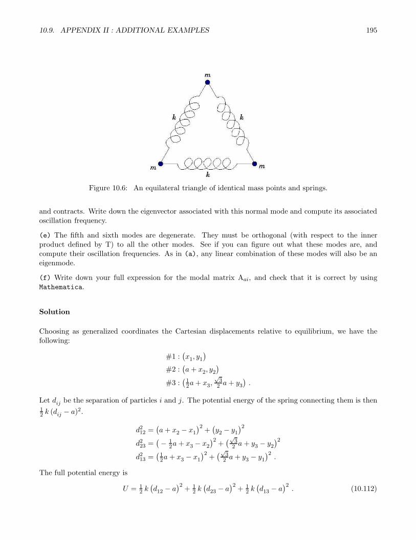
10.9. APPENDIX II : ADDITIONAL EXAMPLES 195
Figure 10.6: An equilateral triangle of identical mass points and springs.
and contracts. Write down the eigenvector associated with this normal mode and compute its associatedoscillation frequency.
(e) The fifth and sixth modes are degenerate. They must be orthogonal (with respect to the innerproduct defined by T) to all the other modes. See if you can figure out what these modes are, andcompute their oscillation frequencies. As in (a), any linear combination of these modes will also be aneigenmode.
(f) Write down your full expression for the modal matrix Aai, and check that it is correct by usingMathematica.
Solution
Choosing as generalized coordinates the Cartesian displacements relative to equilibrium, we have thefollowing:
#1 :(x1, y1
)
#2 :(a+ x2, y2
)
#3 :(12a+ x3,
√32 a+ y3
).
Let dij be the separation of particles i and j. The potential energy of the spring connecting them is then12 k (dij − a)2.
d212 =(a+ x2 − x1
)2+(y2 − y1
)2
d223 =(− 1
2a+ x3 − x2)2
+(√
32 a+ y3 − y2
)2
d213 =(12a+ x3 − x1
)2+(√
32 a+ y3 − y1
)2.
The full potential energy is
U = 12 k(d12 − a
)2+ 1
2 k(d23 − a
)2+ 1
2 k(d13 − a
)2. (10.112)

196 CHAPTER 10. SMALL OSCILLATIONS
Figure 10.7: Zero modes of the mass-spring triangle.
This is a cumbersome expression, involving square roots.
To find T and V, we need to write T and V as quadratic forms, neglecting higher order terms. Therefore,we must expand dij − a to linear order in the generalized coordinates. This results in the following:
d12 = a+(x2 − x1
)+ . . .
d23 = a− 12
(x3 − x2
)+
√32
(y3 − y2
)+ . . .
d13 = a+ 12
(x3 − x1
)+
√32
(y3 − y1
)+ . . . .
Thus,
U = 12 k(x2 − x1
)2+ 1
8 k(x2 − x3 −
√3 y2 +
√3 y3
)2
+ 18 k(x3 − x1 +
√3 y3 −
√3 y1
)2+ higher order terms .
Defining (q1, q2, q3, q4, q5, q6
)=(x1, y1, x2, y2, x3, y3
),
we may now read off
Vσσ′ =∂2U
∂qσ ∂qσ′
∣∣∣∣q
= k
5/4√3/4 −1 0 −1/4 −√
3/4√3/4 3/4 0 0 −√
3/4 −3/4
−1 0 5/4 −√3/4 −1/4
√3/4
0 0 −√3/4 3/4
√3/4 −3/4
−1/4 −√3/4 −1/4
√3/4 1/2 0
−√3/4 −3/4
√3/4 −3/4 0 3/2

10.9. APPENDIX II : ADDITIONAL EXAMPLES 197
Figure 10.8: Finite oscillation frequency modes of the mass-spring triangle.
The T matrix is trivial. From
T = 12m(x21 + y21 + x22 + y22 + x23 + y23
).
we obtain
Tij =∂2T
∂qi ∂qj= mδij ,
and T = m · I is a multiple of the unit matrix.
The zero modes are depicted graphically in figure 10.7. Explicitly, we have
ξx =1√3m
1
0
1
0
1
0
, ξy =1√3m
0
1
0
1
0
1
, ξrot =1√3m
1/2
−√3/2
1/2√3/2
−1
0
.
That these are indeed zero modes may be verified by direct multiplication:
V ξx.y = V ξrot = 0 . (10.113)
The three modes with finite oscillation frequency are depicted graphically in figure 10.8. Explicitly, we

198 CHAPTER 10. SMALL OSCILLATIONS
Figure 10.9: John Henry, statue by Charles O. Cooper (1972). “Now the man that invented the steamdrill, he thought he was mighty fine. But John Henry drove fifteen feet, and the steam drill only madenine.” - from The Ballad of John Henry.
have
ξA =1√3m
−1/2
−√3/2
−1/2√3/2
1
0
, ξB =1√3m
−√3/2
1/2√3/2
1/2
0
−1
, ξdil =1√3m
−√3/2
−1/2√3/2
−1/2
0
1
.
The oscillation frequencies of these modes are easily checked by multiplying the eigenvectors by the matrixV. Since T = m · I is diagonal, we have V ξa = mω2
a ξa. One finds
ωA = ωB =
√3k
2m, ωdil =
√3k
m.
Mathematica? I don’t need no stinking Mathematica.
10.10 Aside : Christoffel Symbols
The coupled equations in eqn. 10.5 may be written in the form
qσ + Γσµν qµ qν = Fσ , (10.114)

10.10. ASIDE : CHRISTOFFEL SYMBOLS 199
with
Γσµν = 1
2 T−1σα
(∂Tαµ∂qν
+∂Tαν∂qµ
− ∂Tµν∂qα
)(10.115)
and
Fσ = −T−1σα
∂U
∂qα. (10.116)
The components of the rank-three tensor Γσαβ are known as Christoffel symbols, in the case where Tµν(q)
defines a metric on the space of generalized coordinates.

200 CHAPTER 10. SMALL OSCILLATIONS

Chapter 11
Elastic Collisions
11.1 Center of Mass Frame
A collision or ‘scattering event’ is said to be elastic if it results in no change in the internal state of anyof the particles involved. Thus, no internal energy is liberated or captured in an elastic process.
Consider the elastic scattering of two particles. Recall the relation between laboratory coordinates r1, r2and the CM and relative coordinates R, r:
R =m1r1 +m2r2m1 +m2
, r1 = R+m2
m1 +m2r
r = r1 − r2 , r2 = R− m1
m1 +m2r
(11.1)
If external forces are negligible, the CM momentum P = MR is constant, and therefore the frame ofreference whose origin is tied to the CM position is an inertial frame of reference. In this frame,
vCM1 =
m2 v
m1 +m2
, vCM2 = − m1 v
m1 +m2
, (11.2)
where v = v1 − v2 = vCM1 − vCM
2 is the relative velocity, which is the same in both L and CM frames.Note that the CM momenta satisfy
pCM1 = m1v
CM1 = µv
pCM2 = m2v
CM2 = −µv ,
(11.3)
where µ = m1m2/(m1 +m2) is the reduced mass. Thus, pCM1 + pCM
2 = 0 and the total momentum in theCM frame is zero. We may then write
pCM1 ≡ p0n , pCM
2 ≡ −p0n ⇒ ECM =p202m1
+p202m2
=p202µ
. (11.4)
201

202 CHAPTER 11. ELASTIC COLLISIONS
Figure 11.1: The scattering of two hard spheres of radii a and b. The scattering angle is χ.
The energy is evaluated when the particles are asymptotically far from each other, in which case thepotential energy is assumed to be negligible. After the collision, energy and momentum conservationrequire
p′1CM ≡ p0n
′ , p′2CM ≡ −p0n′ ⇒ E′CM
= ECM =p202µ
. (11.5)
The angle between n and n′ is the scattering angle χ:
n · n′ ≡ cosχ . (11.6)
The value of χ depends on the details of the scattering process, i.e. on the interaction potential U(r). Asan example, consider the scattering of two hard spheres, depicted in Fig. 11.1. The potential is
U(r) =
∞ if r ≤ a+ b
0 if r > a+ b .(11.7)
Clearly the scattering angle is χ = π−2φ0, where φ0 is the angle between the initial momentum of eithersphere and a line containing their two centers at the moment of contact.
There is a simple geometric interpretation of these results, depicted in Fig. 11.2. We have
p1 = m1V + p0n , p′1 = m1V + p0n′
p2 = m2V − p0n , p′2 = m2V − p0n′ .
(11.8)
So draw a circle of radius p0 whose center is the origin. The vectors p0n and p0n′ must both lie along
this circle. We define the angle ψ between V and n:
V · n = cosψ . (11.9)
It is now an exercise in geometry, using the law of cosines, to determine everything of interest in terms

11.1. CENTER OF MASS FRAME 203
Figure 11.2: Scattering of two particles of masses m1 and m2. The scattering angle χ is the anglebetween n and n′.
of the quantities V , v, ψ, and χ. For example, the momenta are
p1 =
√m2
1 V2 + µ2v2 + 2m1µV v cosψ
p′1 =
√m2
1 V2 + µ2v2 + 2m1µV v cos(χ− ψ)
p2 =
√m2
2 V2 + µ2v2 − 2m2µV v cosψ
p′2 =
√m2
2 V2 + µ2v2 − 2m2µV v cos(χ− ψ) ,
(11.10)
and the scattering angles are
θ1 = tan−1
(µv sinψ
µv cosψ +m1V
)+ tan−1
(µv sin(χ− ψ)
µv cos(χ− ψ) +m1V
)
θ2 = tan−1
(µv sinψ
µv cosψ −m2V
)+ tan−1
(µv sin(χ− ψ)
µv cos(χ− ψ)−m2V
).
(11.11)
If particle 2, say, is initially at rest, the situation is somewhat simpler. In this case, V = m1V /(m1+m2)
and m2V = µv, which means the point B lies on the circle in Fig. 11.3 (m1 6= m2) and Fig. 11.4
(m1 = m2). Let ϑ1,2 be the angles between the directions of motion after the collision and the directionV of impact. The scattering angle χ is the angle through which particle 1 turns in the CM frame. Clearly
tanϑ1 =sinχ
m1m2
+ cosχ, ϑ2 =
12(π − χ) . (11.12)

204 CHAPTER 11. ELASTIC COLLISIONS
Figure 11.3: Scattering when particle 2 is initially at rest.
We can also find the speeds v′1 and v′2 in terms of v and χ, from
p′12= p20 +
(m1m2
p0)2 − 2 m1
m2p20 cos(π − χ) (11.13)
and
p22 = 2 p20 (1− cosχ) . (11.14)
These equations yield
v′1 =
√m2
1 +m22 + 2m1m2 cosχ
m1 +m2v , v′2 =
2m1v
m1 +m2sin(12χ) . (11.15)
The angle ϑmax from Fig. 11.3(b) is given by sinϑmax = m2m1
. Note that when m1 = m2 we haveϑ1 + ϑ2 = π. A sketch of the orbits in the cases of both repulsive and attractive scattering, in both thelaboratory and CM frames, in shown in Fig. 11.5.
Figure 11.4: Scattering of identical mass particles when particle 2 is initially at rest.
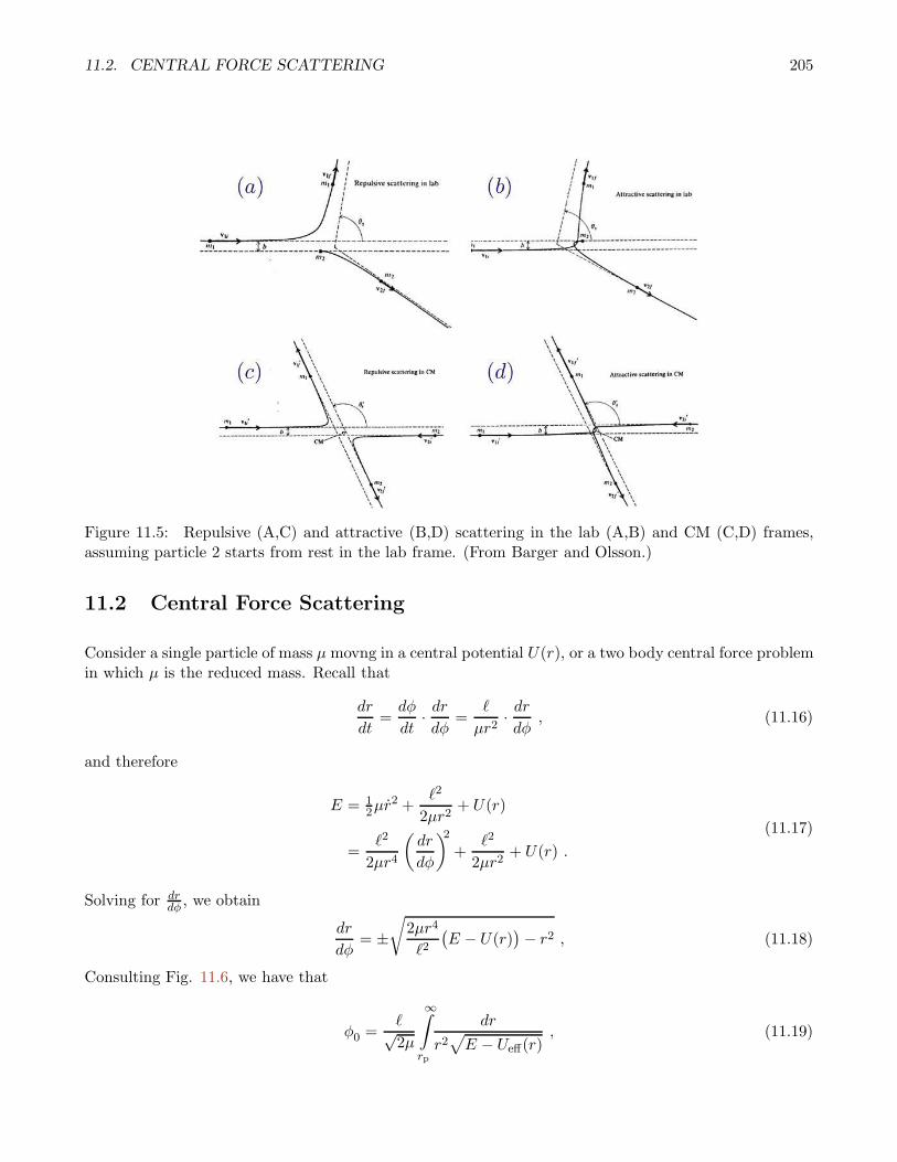
11.2. CENTRAL FORCE SCATTERING 205
Figure 11.5: Repulsive (A,C) and attractive (B,D) scattering in the lab (A,B) and CM (C,D) frames,assuming particle 2 starts from rest in the lab frame. (From Barger and Olsson.)
11.2 Central Force Scattering
Consider a single particle of mass µ movng in a central potential U(r), or a two body central force problemin which µ is the reduced mass. Recall that
dr
dt=dφ
dt· drdφ
=ℓ
µr2· drdφ
, (11.16)
and therefore
E = 12µr
2 +ℓ2
2µr2+ U(r)
=ℓ2
2µr4
(dr
dφ
)2+
ℓ2
2µr2+ U(r) .
(11.17)
Solving for drdφ , we obtain
dr
dφ= ±
√2µr4
ℓ2(E − U(r)
)− r2 , (11.18)
Consulting Fig. 11.6, we have that
φ0 =ℓ√2µ
∞∫
rp
dr
r2√E − Ueff(r)
, (11.19)

206 CHAPTER 11. ELASTIC COLLISIONS
Figure 11.6: Scattering in the CM frame. O is the force center and P is the point of periapsis. Theimpact parameter is b, and χ is the scattering angle. φ0 is the angle through which the relative coordinatemoves between periapsis and infinity.
where rp is the radial distance at periapsis, and where
Ueff(r) =ℓ2
2µr2+ U(r) (11.20)
is the effective potential, as before. From Fig. 11.6, we conclude that the scattering angle is
χ =∣∣π − 2φ0
∣∣ . (11.21)
It is convenient to define the impact parameter b as the distance of the asymptotic trajectory from aparallel line containing the force center. The geometry is shown again in Fig. 11.6. Note that the energyand angular momentum, which are conserved, can be evaluated at infinity using the impact parameter:
E = 12µv
2∞ , ℓ = µv∞b . (11.22)
Substituting for ℓ(b), we have
φ0(E, b) =
∞∫
rp
dr
r2b√
1− b2
r2− U(r)
E
, (11.23)
In physical applications, we are often interested in the deflection of a beam of incident particles by ascattering center. We define the differential scattering cross section dσ by
dσ =# of particles scattered into solid angle dΩ per unit time
incident flux. (11.24)
Now for particles of a given energy E there is a unique relationship between the scattering angle χ andthe impact parameter b, as we have just derived in eqn. 11.23. The differential solid angle is given bydΩ = 2π sinχdχ, hence
dσ
dΩ=
b
sinχ
∣∣∣∣db
dχ
∣∣∣∣ =∣∣∣∣d (12b
2)
d cosχ
∣∣∣∣ . (11.25)

11.2. CENTRAL FORCE SCATTERING 207
Figure 11.7: Geometry of hard sphere scattering.
Note that dσdΩ has dimensions of area. The integral of dσ
dΩ over all solid angle is the total scattering cross
section,
σT = 2π
π∫
0
dχ sinχdσ
dΩ. (11.26)
11.2.1 Hard sphere scattering
Consider a point particle scattering off a hard sphere of radius a, or two hard spheres of radii a1 and a2scattering off each other, with a ≡ a1 + a2. From the geometry of Fig. 11.7, we have b = a sinφ0 and
φ0 =12(π − χ), so
b2 = a2 sin2(12π − 1
2χ) =12a
2 (1 + cosχ) . (11.27)
We therefore havedσ
dΩ=d (12b
2)
d cos χ= 1
4 a2 (11.28)
and σT = πa2. The total scattering cross section is simply the area of a sphere of radius a projected ontoa plane perpendicular to the incident flux.
11.2.2 Rutherford scattering
Consider scattering by the Kepler potential U(r) = −kr . We assume that the orbits are unbound, i.e.
they are Keplerian hyperbolae with E > 0, described by the equation
r(φ) =a (ε2 − 1)
±1 + ε cosφ⇒ cosφ0 = ± 1
ε. (11.29)
Recall that the eccentricity is given by
ε2 = 1 +2Eℓ2
µk2= 1 +
(µbv∞k
)2. (11.30)

208 CHAPTER 11. ELASTIC COLLISIONS
We then have(µbv∞k
)2= ε2 − 1
= sec2φ0 − 1 = tan2φ0 = ctn2(12χ).
(11.31)
Therefore
b(χ) =k
µv2∞ctn(12χ)
(11.32)
We finally obtain
dσ
dΩ=d (12b
2)
d cos χ=
1
2
(k
µv2∞
)2 d ctn2(12χ)
d cosχ
=1
2
(k
µv2∞
)2 d
d cosχ
(1 + cosχ
1− cosχ
)
=
(k
2µv2∞
)2csc4
(12χ),
(11.33)
which is the same asdσ
dΩ=
(k
4E
)2csc4
(12χ). (11.34)
Since dσdΩ ∝ χ−4 as χ → 0, the total cross section σT diverges! This is a consequence of the long-ranged
nature of the Kepler/Coulomb potential. In electron-atom scattering, the Coulomb potential of thenucleus is screened by the electrons of the atom, and the 1/r behavior is cut off at large distances.
11.2.3 Transformation to laboratory coordinates
We previously derived the relation
tanϑ =sinχ
γ + cosχ, (11.35)
where ϑ ≡ ϑ1 is the scattering angle for particle 1 in the laboratory frame, and γ = m1m2
is the ratio ofthe masses. We now derive the differential scattering cross section in the laboratory frame. To do so, wenote that particle conservation requires
(dσ
dΩ
)
L
· 2π sinϑ dϑ =
(dσ
dΩ
)
CM
· 2π sinχdχ , (11.36)
which says (dσ
dΩ
)
L
=
(dσ
dΩ
)
CM
· d cosχ
d cos ϑ. (11.37)
From
cos ϑ =1√
1 + tan2ϑ
=γ + cosχ√
1 + γ2 + 2γ cosχ,
(11.38)

11.2. CENTRAL FORCE SCATTERING 209
we derived cos ϑ
d cosχ=
1 + γ cosχ(1 + γ2 + 2γ cosχ
)3/2 (11.39)
and, accordingly,(dσ
dΩ
)
L
=
(1 + γ2 + 2γ cosχ
)3/2
1 + γ cosχ·(dσ
dΩ
)
CM
. (11.40)