Optimization of Design

Lecturer：Dung-An WangLecture 8

2

Lecture outline

Reading: Ch8 of textToday’s lecture

3

8.1 LINEAR FUNCTIONS

Cost Function

Constraints

4

8.2 The standard LP problem Only equality constraints are treated in standard linear

programming

5

Summation Form of the Standard LP Problem

6

Matrix Form of the Standard LP Problem

7

8.2.2 Transcription to Standard LP

Non-Negative Constraint Limits Treatment of “<= Type”Constraints

Treatment of “>= Type”Constraints

8

Unrestricted Variables

Require that all design variables to be nonnegative inthe standard LP problem

If a design variable xj is unrestricted in sign, it canalways be written as the difference of two non-negativevariables

9

EXAMPLE 8.1 CONVERSION TO STANDARD LP FORM

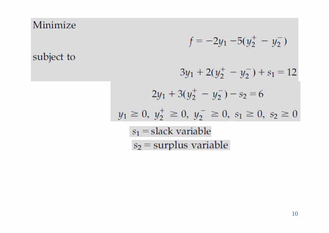
10

11

BASIC CONCEPTS

the optimum solution for the LP problem always lies onthe boundary of the feasible set.

The solution is at least at one of the vertices of theconvex feasible set (called the convex polyhedral set).

12

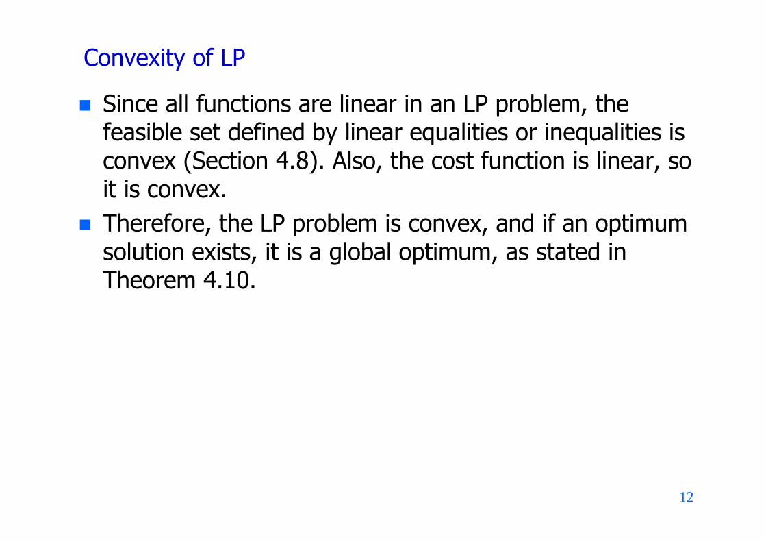
Convexity of LP

Since all functions are linear in an LP problem, thefeasible set defined by linear equalities or inequalities isconvex (Section 4.8). Also, the cost function is linear, soit is convex.

Therefore, the LP problem is convex, and if an optimumsolution exists, it is a global optimum, as stated inTheorem 4.10.

13

Write the linear system in a tableau

14

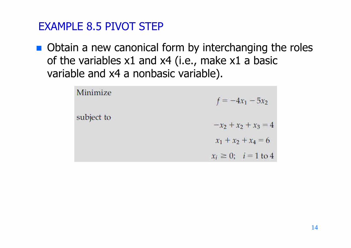
EXAMPLE 8.5 PIVOT STEP

Obtain a new canonical form by interchanging the rolesof the variables x1 and x4 (i.e., make x1 a basicvariable and x4 a nonbasic variable).

15

16

Simplex method

Searches through only the basic feasible solutions andstops once an optimum solution is obtained

17

Determine three basic solutions using the Gauss-Jordanelimination method

18

19

20

21

8.5 THE SIMPLEX METHOD

EXAMPLE 8.7 STEPS OF THE SIMPLEX METHOD

22

The graphical solution to the problem

Optimum solution along line CD. z*=4.

23

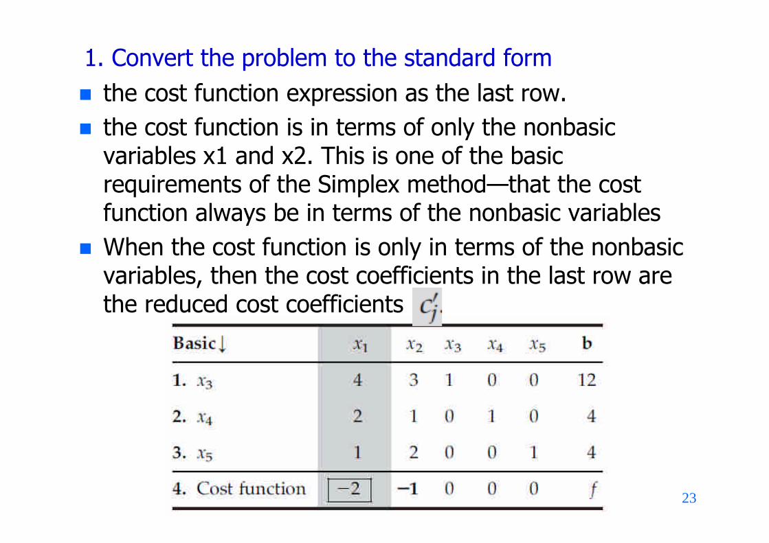
1. Convert the problem to the standard form the cost function expression as the last row. the cost function is in terms of only the nonbasic

variables x1 and x2. This is one of the basicrequirements of the Simplex method—that the costfunction always be in terms of the nonbasic variables

When the cost function is only in terms of the nonbasicvariables, then the cost coefficients in the last row arethe reduced cost coefficients

24

2. Initial basic feasible solution

25

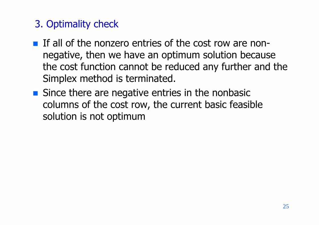
3. Optimality check

If all of the nonzero entries of the cost row are non-negative, then we have an optimum solution becausethe cost function cannot be reduced any further and theSimplex method is terminated.

Since there are negative entries in the nonbasiccolumns of the cost row, the current basic feasiblesolution is not optimum

26

4. Selection of a nonbasic variable to become basic

Select a variable associated with the smallest value inthe cost row

27

5. Selection of a basic variable to become nonbasic Selection of the row with the smallest ratio as the pivot

row maintains the feasibility of the new basic solution(all xi >= 0).

28

6. Pivot step

29

7. Optimum solution

This solution is identified as point D in the figure. Wesee that the cost function has been reduced from 0 to-4. The coefficients in the nonbasic columns of the lastrow are non-negative

so no further reduction of the cost function is possible. Thus, the foregoing solution is the optimum point. Note

that for this example, only one iteration of the Simplexmethod gave the optimum solution. In general, moreiterations are needed until all coefficients in the costrow become non-negative

30

EXAMPLE 8.8 SOLUTION BY THE SIMPLEX METHOD

31

32

33

34

8.6.1 Artificial Variables

When there are “>= type”constraints in the linearprogramming problem, surplus variables are subtractedfrom them to transform the problem into the standardform. The equality constraints, if present, are notchanged because they are already in the standard form.For such problems, an initial basic feasible solutioncannot be obtained by selecting the original designvariables as nonbasic (setting them to zero), as is thecase when there are only “<= type”constraints.

To obtain an initial basic feasible solution, the Gauss-Jordan elimination procedure can be used to convertAx=b to the canonical form.

35

However, an easier way is to introduce non-negativeauxiliary variables for the “>= type”and equalityconstraints, define an auxiliary LP problem, and solve itusing the Simplex method.

The auxiliary variables are called artificial variables.These are variables in addition to the surplus variablesfor the “>= type”constraints.

They have no physical meaning, but with their additionwe obtain an initial basic feasible solution for theauxiliary LP problem by treating the artificial variablesas basic along with any slack variables for the “<=type”constraints. All other variables are treated asnonbasic (i.e., set to zero).

36

EXAMPLE 8.12 INTRODUCTION OF ARTIFICIALVARIABLES

37

standard form

38

canonical form

introduce non-negative artificial variables

39

8.6.2 Artificial Cost Function

The artificial variable for each equality and “>= type”constraint is introduced to obtain an initial basic feasiblesolution for the auxiliary problem. These variables haveno physical meaning and need to be eliminated fromthe problem.

To eliminate the artificial variables from the problem,we define an auxiliary cost function called the artificialcost function and minimize it subject to the constraintsof the problem and the non-negativity of all of thevariables.

40

The artificial cost function is simply a sum of all theartificial variables and will be designated as w

41

8.6.3 Definition of the Phase I Problem

Since the artificial variables are introduced simply toobtain an initial basic feasible solution for the originalproblem, they need to be eliminated eventually. Thiselimination is done by defining and solving an LPproblem called the Phase I problem.

The objective of this problem is to make all the artificialvariables nonbasic so they have zero value.

42

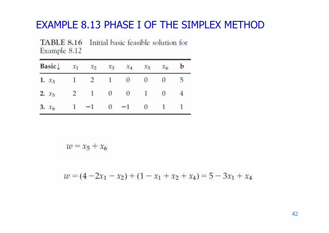
EXAMPLE 8.13 PHASE I OF THE SIMPLEX METHOD

43

EXAMPLE 8.13 PHASE I OF THE SIMPLEX METHOD

44

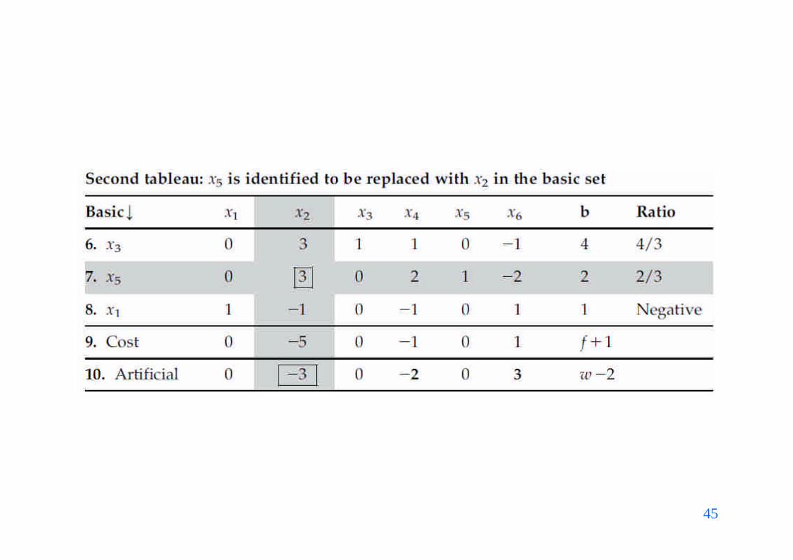
Now the Simplex iterations are carried out using theartificial cost row to determine the pivot element.

In the initial tableau, the element a31=1 is identified asthe pivot element

45

46

47

Since both of the artificial variables have becomenonbasic, the artificial cost function has attained a zerovalue. This indicates the end of Phase I of the Simplexmethod.

Now we can discard the artificial cost row and theartificial variable columns x5 and x6 in Table 8.17 andcontinue with the Simplex iterations using the real costrow to determine the pivot column.

48

EXAMPLE 8.14 USE OF ARTIFICIAL VARIABLES FOR“>= TYPE”CONSTRAINTS

49

50

51