Embed Size (px)
Citation preview
Lecturer’s desk
Physics- atmospheric Sciences (PAS) - Room 201
s c r e e ns c r e e n
Row A
Row B
Row C
Row D
Row E
Row F
Row G
Row H
13 12 11 10 9 8 7 Row A
14 13 12 11 10 9 8 7 Row B
15 14 13 12 11 10 9 8 7 Row C
15 14 13 12 11 10 9 8 7 Row D16
15 14 13 12 11 10 9 8 7 Row E17 16
15 14 13 12 11 10 9 8 7 Row F17 16
15 14 13 12 11 10 9 8 7 Row G17 16
15 14 13 12 11 10 9 8 7 Row H16
18
table
Row A
Row B
Row C
Row D
Row E
Row F
Row G
Row H
15 1417 161819
16 1518 171920
17 1619 182021
18 1720 192122
19 1821 202223
20 1922 212324
18 1720 192122
19 1821 202223
2 14 356
2 14 356
2 14 356
2 14 356
2 14 356
2 14 356
2 14 356
2 14 356
Row J
Row K
Row L
Row M
Row N
Row P2 14 35
2 14 35
2 14 35
2 14 35
2 14 35
15Row J
Row K
Row L
Row M
Row N
Row P
27 2629 2830
25 2427 2628
24 2326 2527
23 2225 2426
25 2427 2628
27 2629 2830
614 13 12 11 10 9 8 716 1518 1719202122
614 13 12 11 10 9 8 716 1518 171920212223
614 13 12 11 10 9 8 716 1518 171920212223
614 13 12 11 10 9 8 71624 18 171920212223 1525
614 13 12 11 10 9 8 71624 18 171920212223 1525
Row Q2 14 3527 2629 2830 614 13 12 11 10 9 8 724 2223 21 - 152537 3639 3840 34 31323335
69 8 713 table1418192021
Hand in
(Optional)
Revised
Memo
MGMT 276: Statistical Inference in Management
Fall 2015
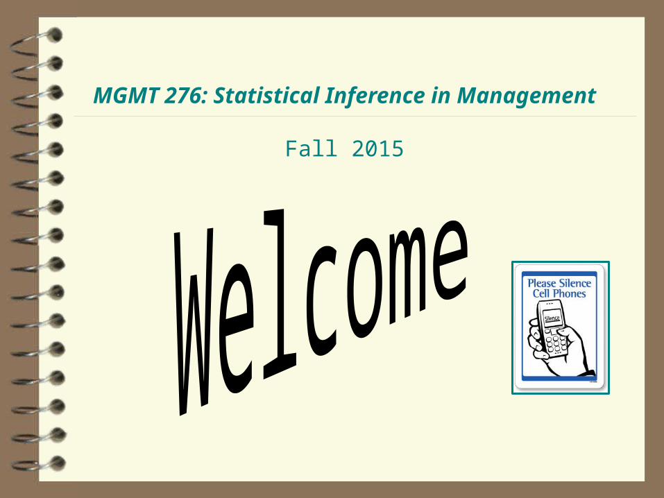
We’ll be starting
this today

Just for Fun AssignmentsGo to D2L - Click on “Content”
Click on “Interactive Online Just-for-fun Assignments”Complete Assignments 1 – 7
Please note: These are not worth any class points and are different from the required homeworks
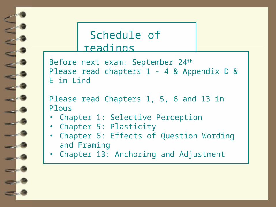
Schedule of readings
Before next exam: September 24th Please read chapters 1 - 4 & Appendix D & E in Lind
Please read Chapters 1, 5, 6 and 13 in Plous• Chapter 1: Selective Perception• Chapter 5: Plasticity• Chapter 6: Effects of Question Wording and Framing• Chapter 13: Anchoring and Adjustment
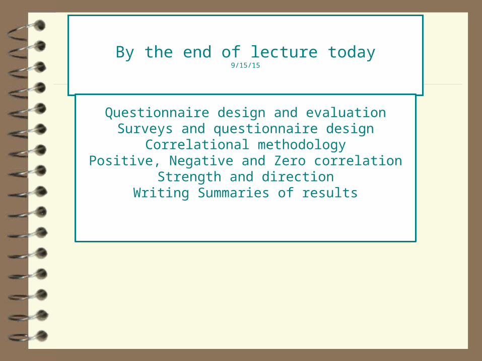
By the end of lecture today9/15/15
Questionnaire design and evaluationSurveys and questionnaire design
Correlational methodologyPositive, Negative and Zero correlation
Strength and directionWriting Summaries of results

Homework Assignment
Assignment 4Describing Data Visually using MS Excel
Due: Thursday, September 17th
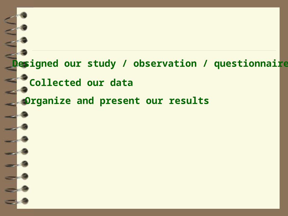
Designed our study / observation / questionnaire
Collected our data
Organize and present our results
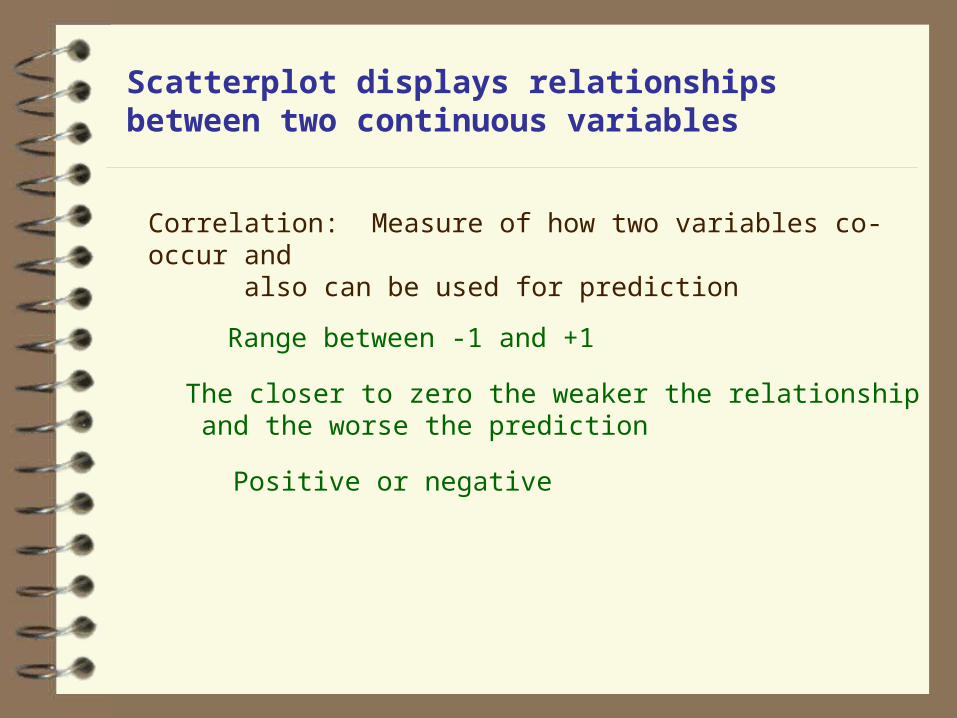
Scatterplot displays relationships between two continuous variables
Correlation: Measure of how two variables co-occur and also can be used for prediction
Range between -1 and +1
The closer to zero the weaker the relationshipand the worse the prediction
Positive or negative
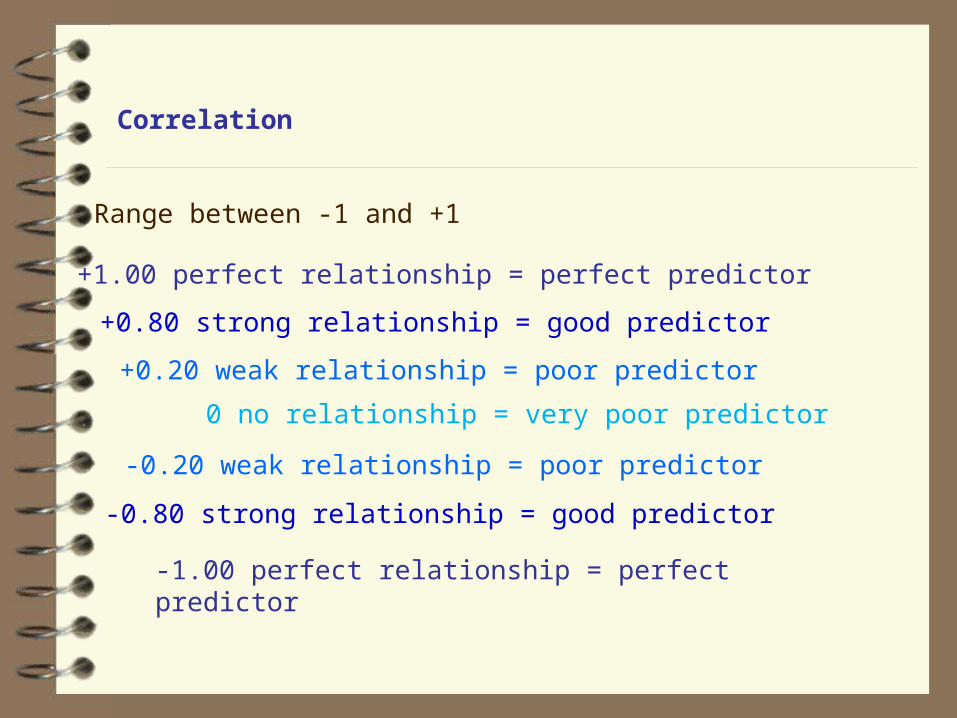
Correlation
Range between -1 and +1
-1.00 perfect relationship = perfect predictor
+1.00 perfect relationship = perfect predictor
0 no relationship = very poor predictor
+0.80 strong relationship = good predictor
-0.80 strong relationship = good predictor
+0.20 weak relationship = poor predictor
-0.20 weak relationship = poor predictor
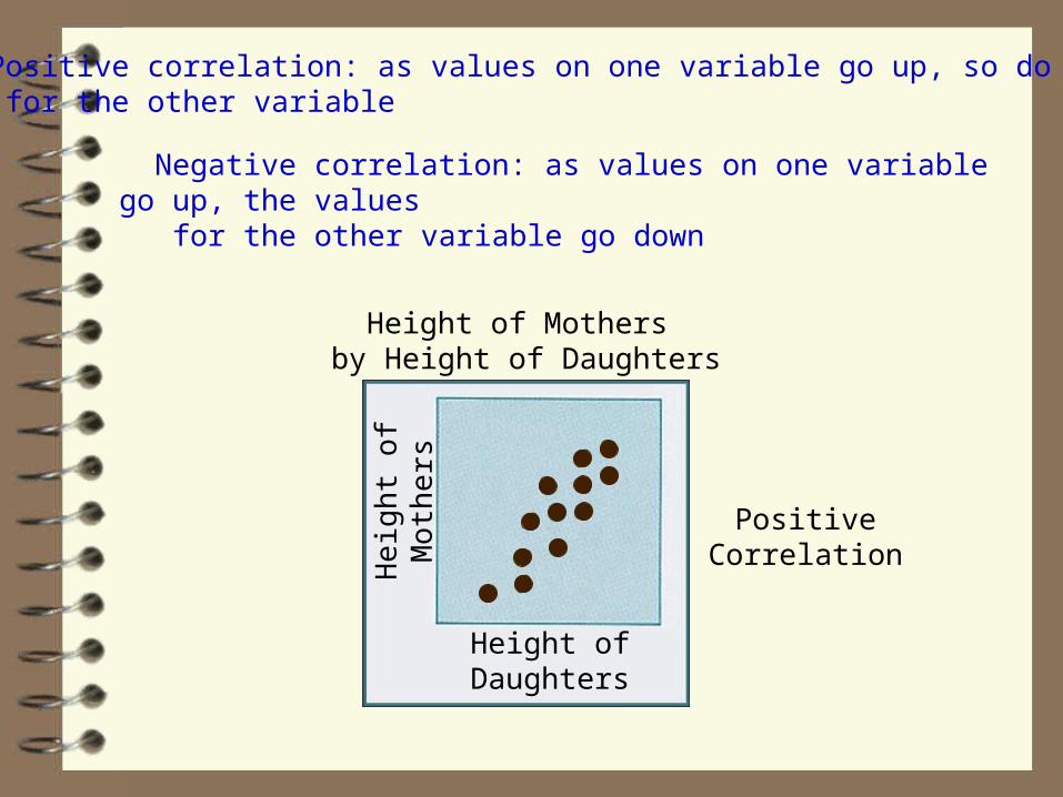
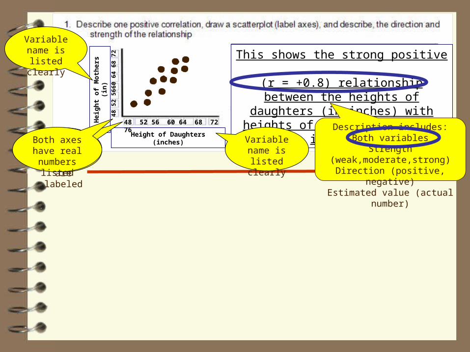
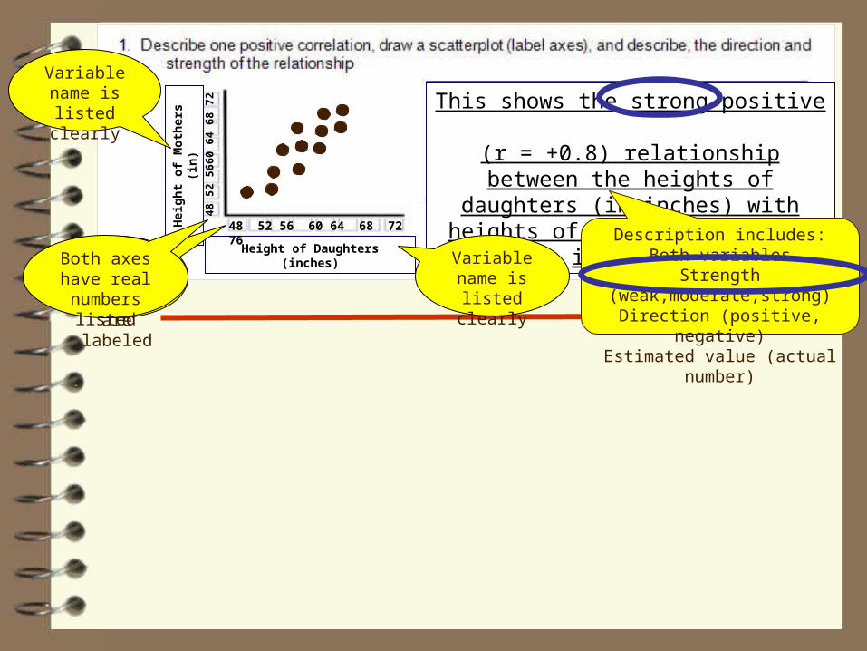
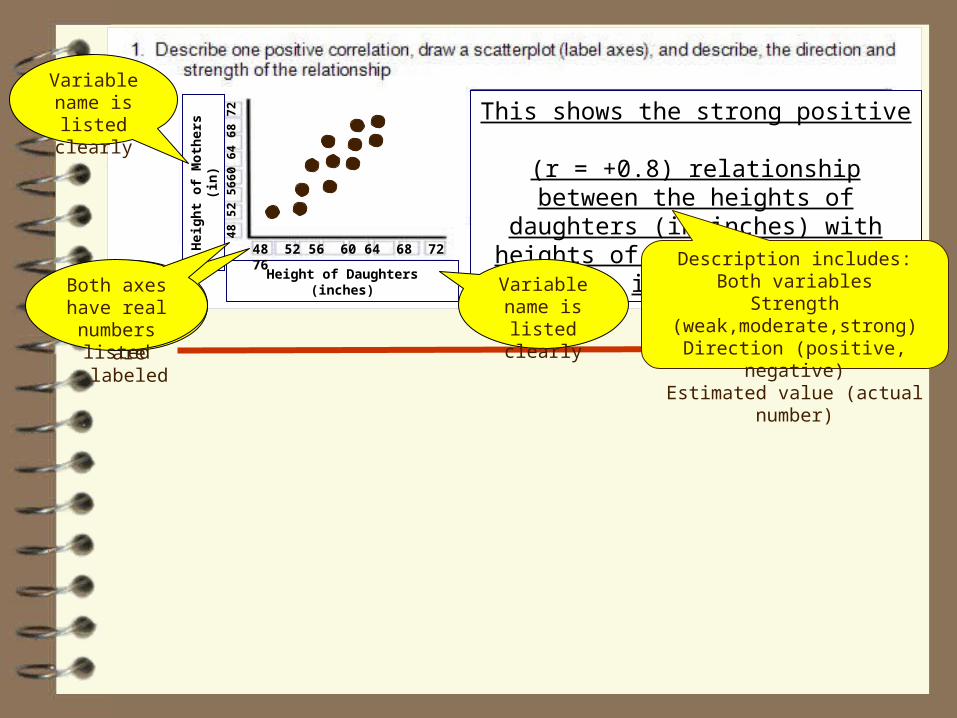
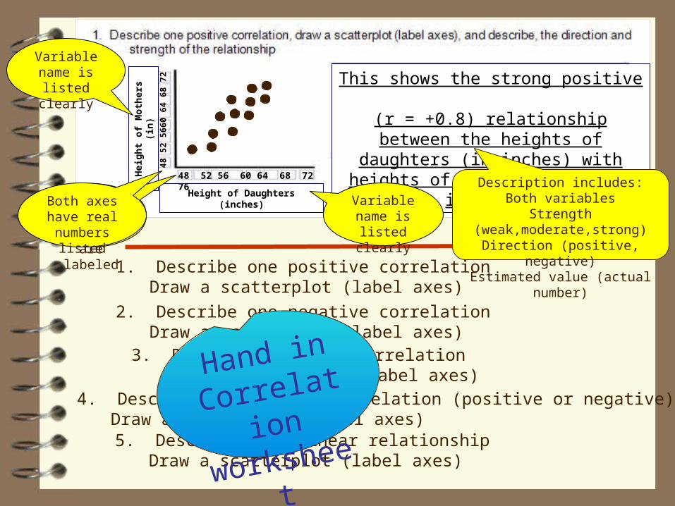
Height of Mothers by Height of Daughters
PositiveCorrelation
Height ofDaughters
Heig
ht
of
Moth
ers
Positive correlation: as values on one variable go up, so do valuesfor the other variable
Negative correlation: as values on one variable go up, the values
for the other variable go down
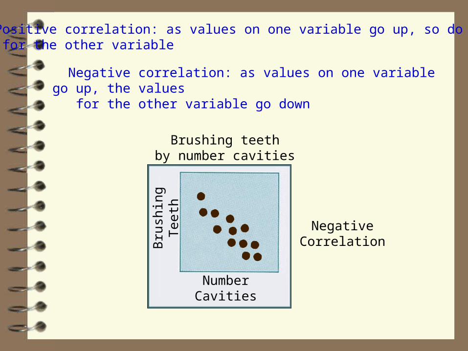
Brushing teethby number cavities
NegativeCorrelation
NumberCavities
Bru
shin
gTe
eth
Positive correlation: as values on one variable go up, so do valuesfor the other variable
Negative correlation: as values on one variable go up, the values
for the other variable go down
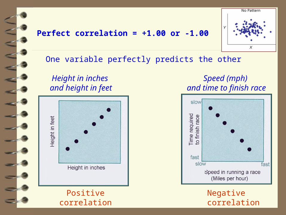
Perfect correlation = +1.00 or -1.00
One variable perfectly predicts the other
Negativecorrelation
Positivecorrelation
Height in inches and height in feet
Speed (mph) and time to finish
race
Correlation
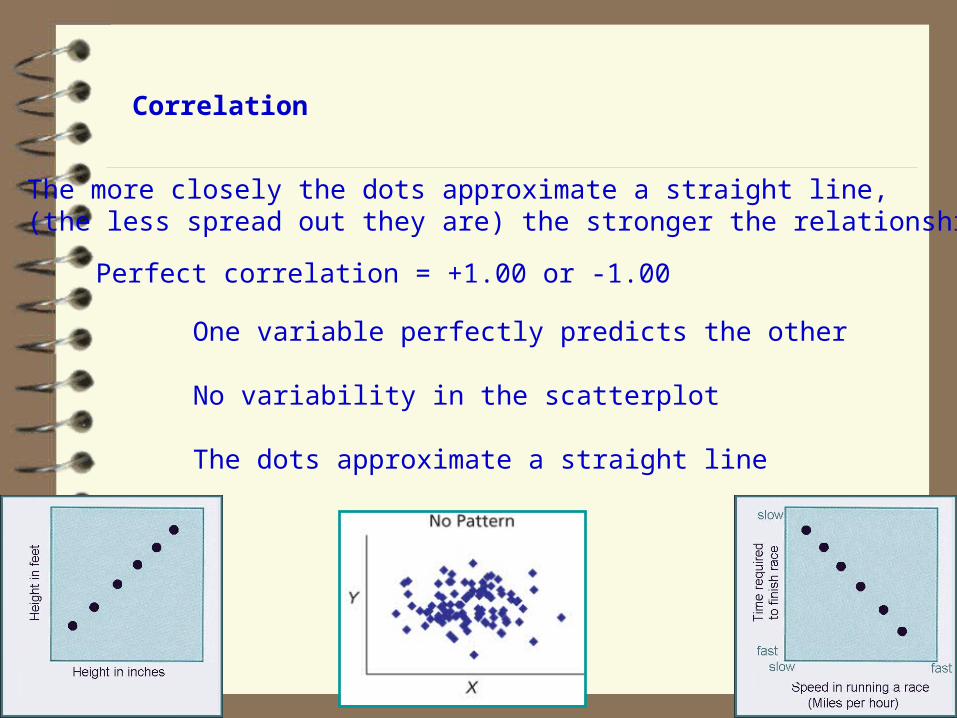
Perfect correlation = +1.00 or -1.00
The more closely the dots approximate a straight line,(the less spread out they are) the stronger the relationship is.
One variable perfectly predicts the other
No variability in the scatterplot
The dots approximate a straight line

Correlation
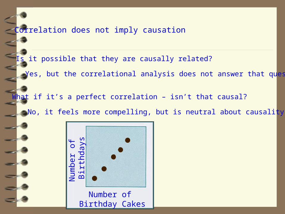
Is it possible that they are causally related?
Correlation does not imply causation
Yes, but the correlational analysis does not answer that question
What if it’s a perfect correlation – isn’t that causal?
No, it feels more compelling, but is neutral about causality
Number of Birthday Cakes
Nu
mb
er
of
Bir
thd
ays
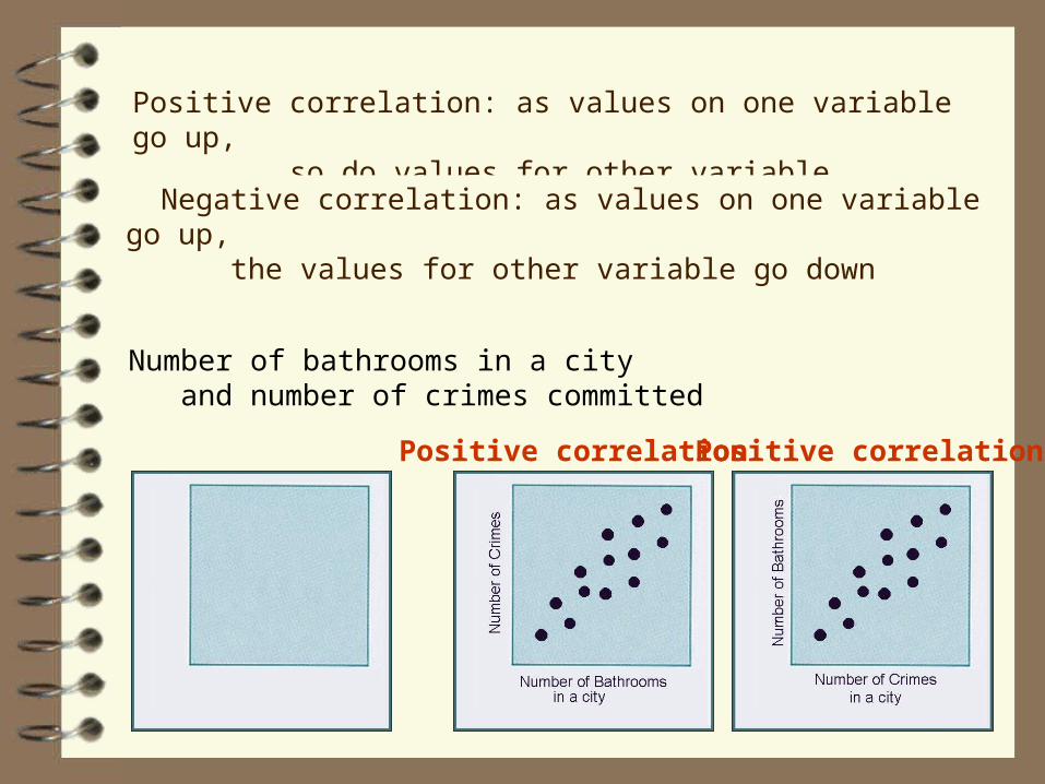
Number of bathrooms in a city and number of crimes committed
Positive correlationPositive correlation
Positive correlation: as values on one variable go up,
so do values for other variable
Negative correlation: as values on one variable go up, the values for other variable go down
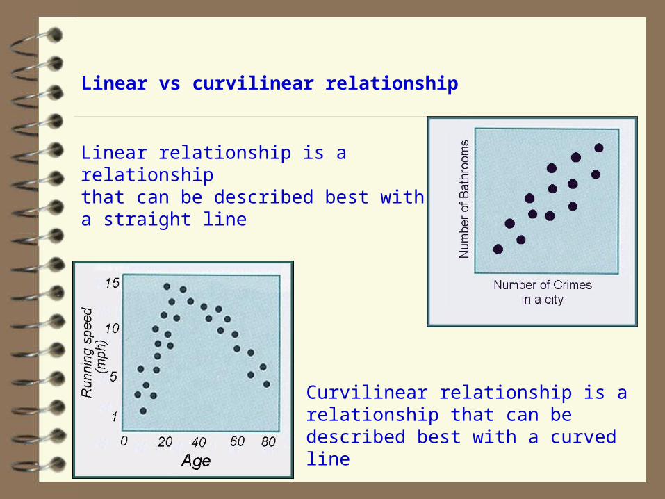
Linear vs curvilinear relationship
Linear relationship is a relationshipthat can be described best with a straight line
Curvilinear relationship is a relationship that can be described best with a curved line
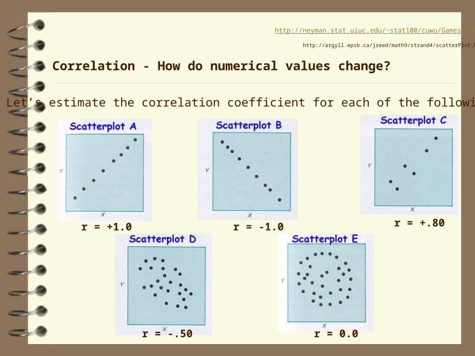
Correlation - How do numerical values change?
Let’s estimate the correlation coefficient for each of the following
r = +1.0 r = -1.0 r = +.80
r = -.50 r = 0.0
http://neyman.stat.uiuc.edu/~stat100/cuwu/Games.html
http://argyll.epsb.ca/jreed/math9/strand4/scatterPlot.htm
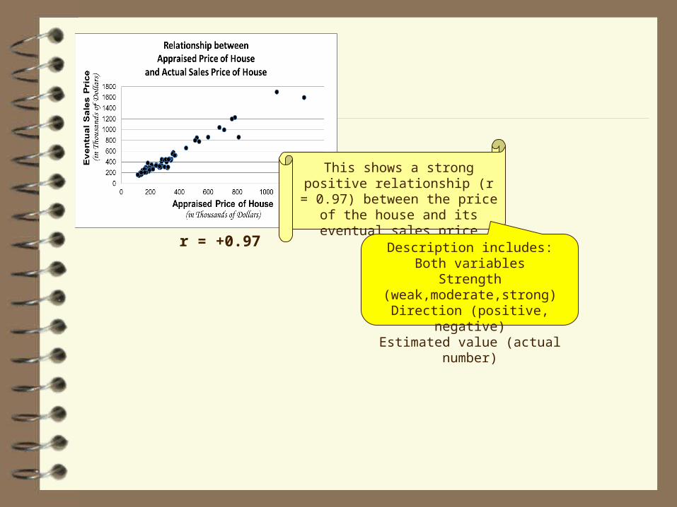
r = +0.97
This shows a strong positive relationship (r = 0.97)
between the price of the house and its eventual sales
priceDescription includes:
Both variablesStrength
(weak,moderate,strong)Direction (positive, negative)
Estimated value (actual number)
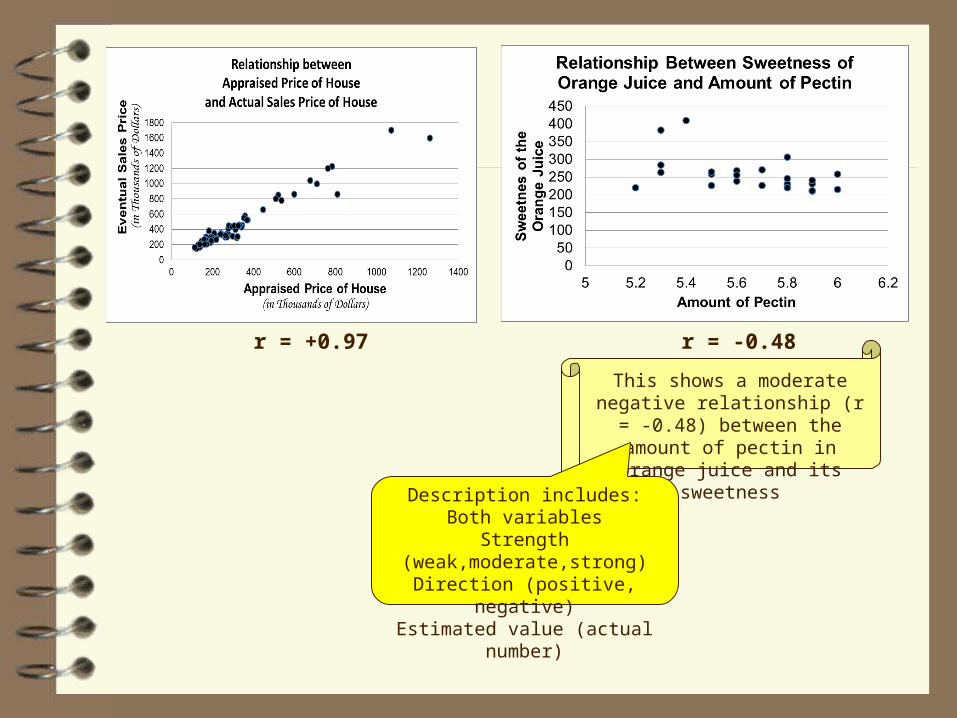
r = +0.97 r = -0.48
This shows a moderate negative relationship (r = -
0.48) between the amount of pectin in orange juice and its
sweetnessDescription includes:
Both variablesStrength
(weak,moderate,strong)Direction (positive, negative)
Estimated value (actual number)
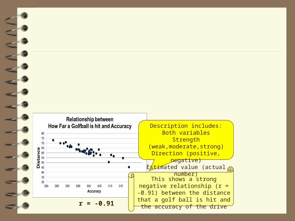
r = -0.91
This shows a strong negative relationship (r = -0.91) between the distance that a golf ball is
hit and the accuracy of the drive
Description includes:Both variables
Strength (weak,moderate,strong)
Direction (positive, negative)Estimated value (actual
number)
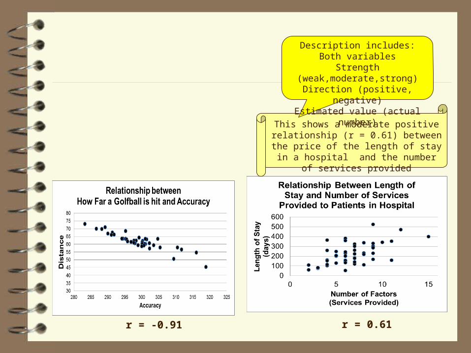
r = -0.91 r = 0.61
This shows a moderate positive relationship (r = 0.61) between the
price of the length of stay in a hospital and the number of services
provided
Description includes:Both variables
Strength (weak,moderate,strong)
Direction (positive, negative)Estimated value (actual
number)
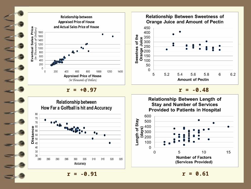
r = +0.97 r = -0.48
r = -0.91 r = 0.61
Height of Daughters (inches)
Heig
ht
of
Moth
ers
(i
n)
48 52 56 60 64 68 72 76 48 5
2 5
660 6
4 6
8 7
2
This shows the strong positive (r = +0.8) relationship between the
heights of daughters (in inches) with heights of their mothers (in
inches).
Both axes and values are labeled
Both axes have real numbers
listed
Variable name is
listed clearly
Variable name is listed clearly
Description includes:Both variables
Strength (weak,moderate,strong)
Direction (positive, negative)Estimated value (actual
number)
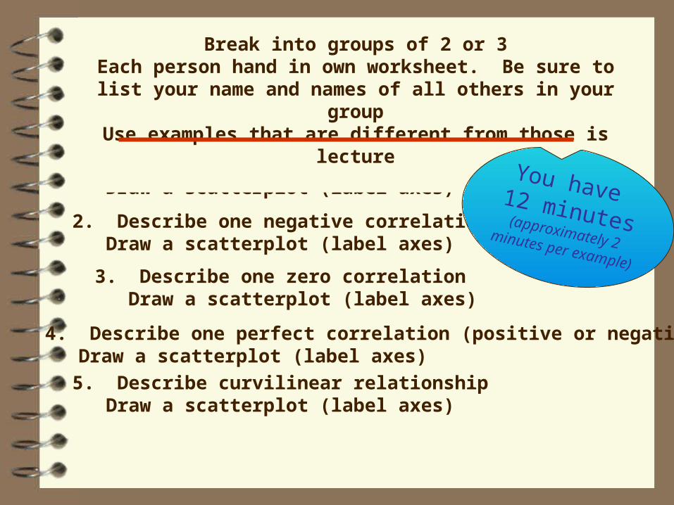
1. Describe one positive correlationDraw a scatterplot (label axes)
2. Describe one negative correlationDraw a scatterplot (label axes)
3. Describe one zero correlationDraw a scatterplot (label axes)
Break into groups of 2 or 3Each person hand in own worksheet. Be sure to list
your name and names of all others in your groupUse examples that are different from those is lecture
4. Describe one perfect correlation (positive or negative)Draw a scatterplot (label axes)
5. Describe curvilinear relationshipDraw a scatterplot (label axes)
You have 12 minutes(approximately 2 minutes per example)
Height of Daughters (inches)
Heig
ht
of
Moth
ers
(i
n)
48 52 56 60 64 68 72 76 48 5
2 5
660 6
4 6
8 7
2
This shows the strong positive (r = +0.8) relationship between the
heights of daughters (in inches) with heights of their mothers (in
inches).
Both axes and values are labeled
Both axes have real numbers
listed
1. Describe one positive correlationDraw a scatterplot (label axes)
2. Describe one negative correlationDraw a scatterplot (label axes)
3. Describe one zero correlationDraw a scatterplot (label axes)
4. Describe one perfect correlation (positive or negative)Draw a scatterplot (label axes)
5. Describe curvilinear relationshipDraw a scatterplot (label axes)
Variable name is
listed clearly
Variable name is listed clearly
Description includes:Both variables
Strength (weak,moderate,strong)
Direction (positive, negative)Estimated value (actual
number)
Hand in
Correlatio
n
worksheet
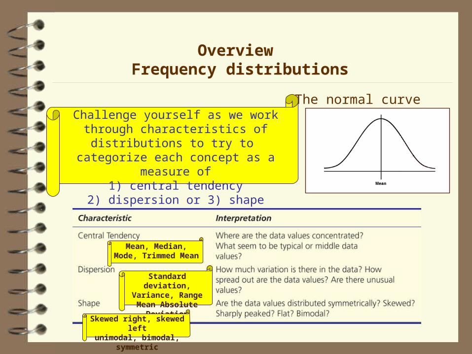
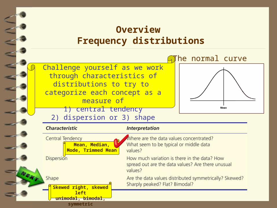
Overview Frequency distributions
The normal curve
Mean, Median,Mode, Trimmed Mean
Standard deviation,Variance, Range
Mean Absolute Deviation
Skewed right, skewed leftunimodal, bimodal, symmetric
Challenge yourself as we work through characteristics of distributions to try to categorize each concept as a measure
of 1) central tendency
2) dispersion or 3) shape
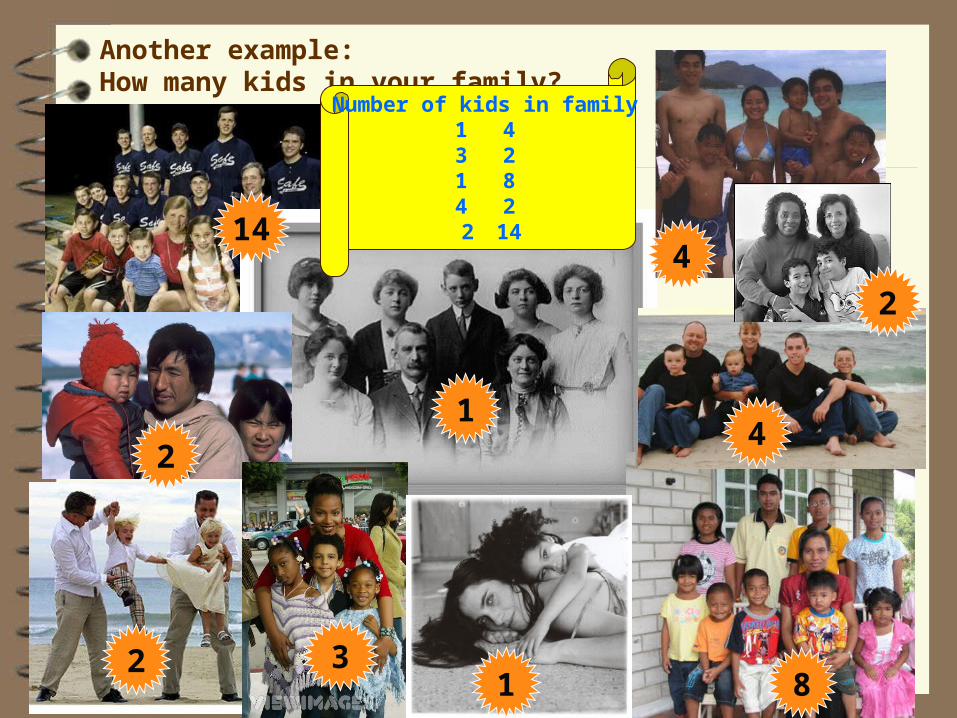
Another example: How many kids in your family?
3
4
82
2
1
4
1
14
2
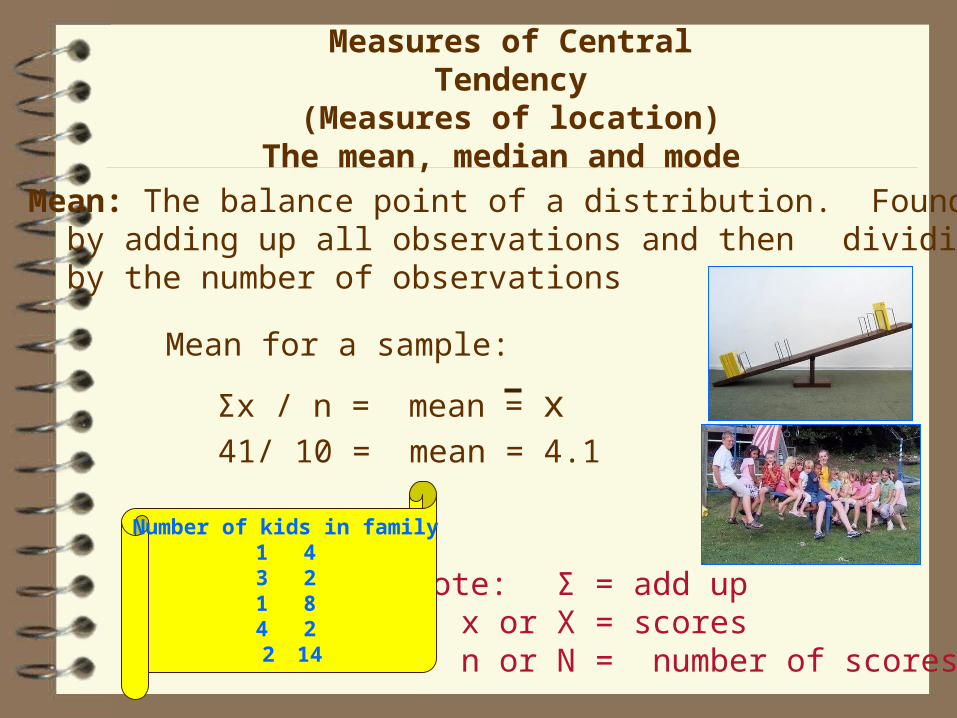
Number of kids in family1 43 21 84 2 2 14
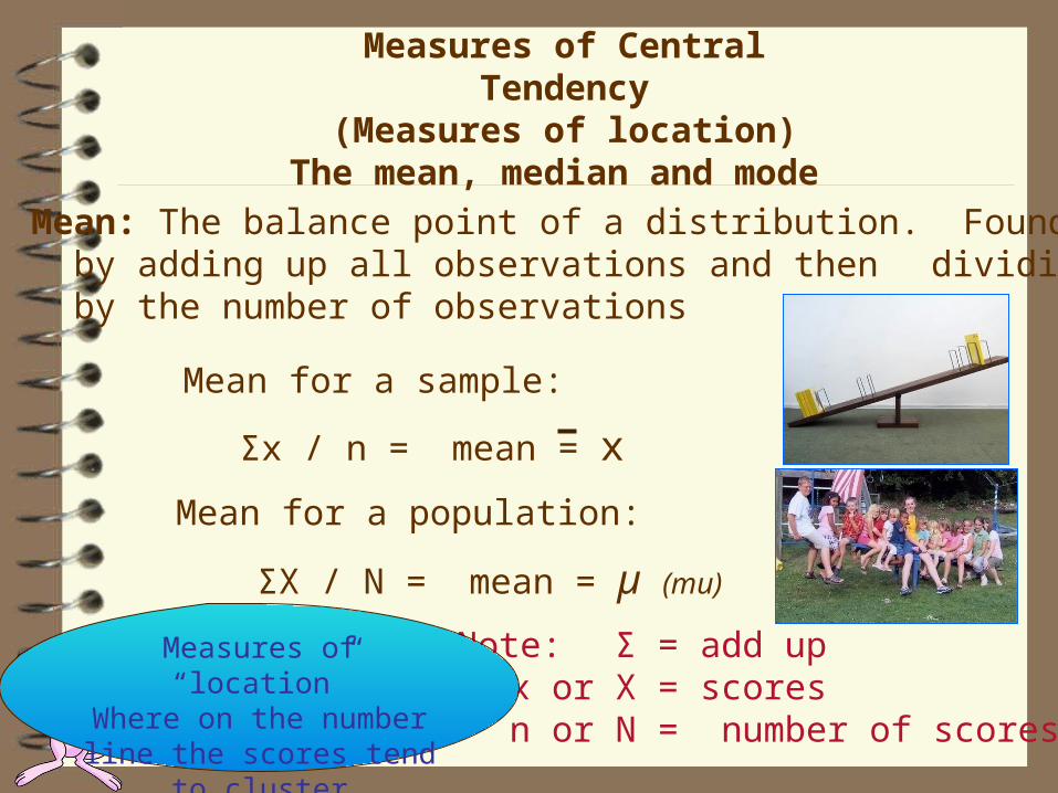
Measures of Central Tendency(Measures of location)
The mean, median and mode
Mean: The balance point of a distribution. Found by adding up all observations and then dividing by the number of observations
Mean for a sample:
Mean for a population:
ΣX / N = mean = µ (mu)
Note: Σ = add upx or X = scoresn or N = number of scores
Σx / n = mean = x
Measures of “location”Where on the number line the scores tend to
cluster
Measures of Central Tendency(Measures of location)
The mean, median and mode
Mean: The balance point of a distribution. Found by adding up all observations and then dividing by the number of observations
Mean for a sample:
Note: Σ = add upx or X = scoresn or N = number of scores
Σx / n = mean = x
Number of kids in family1 43 21 84 2 2 14
41/ 10 = mean = 4.1
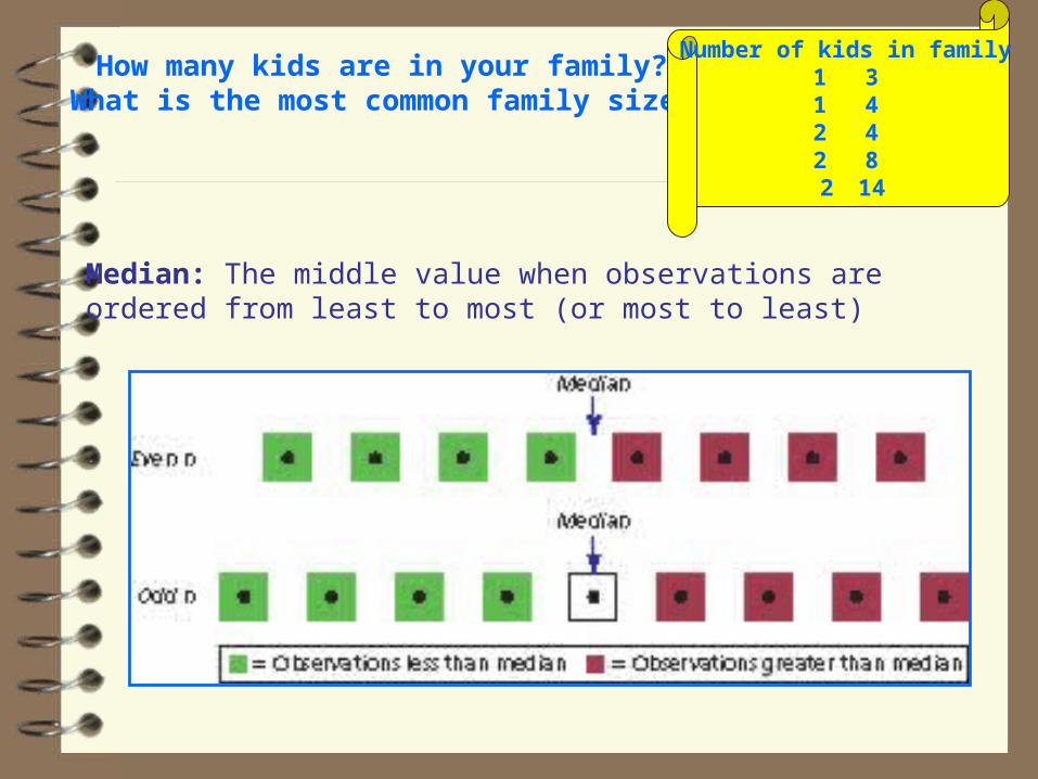
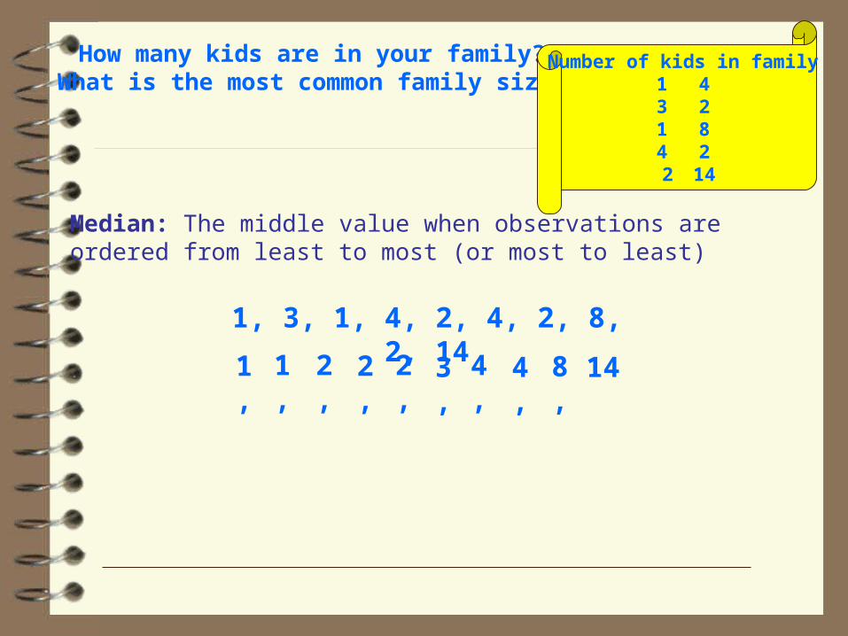
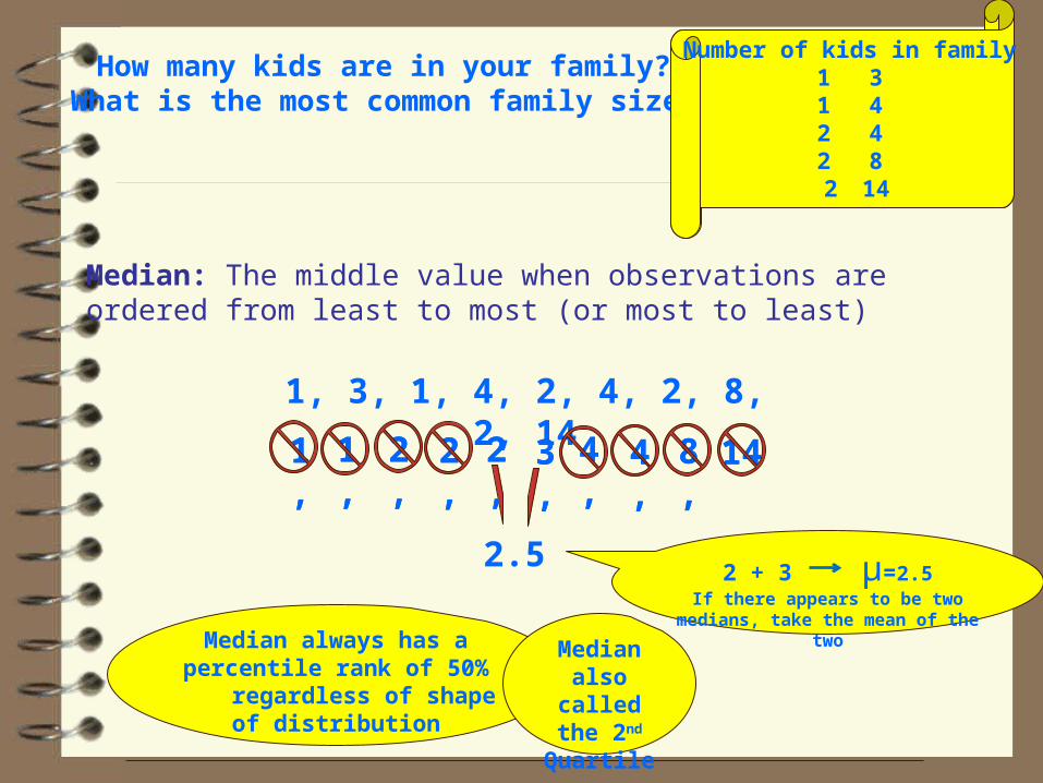
How many kids are in your family?What is the most common family size?
Number of kids in family1 31 42 42 8 2 14
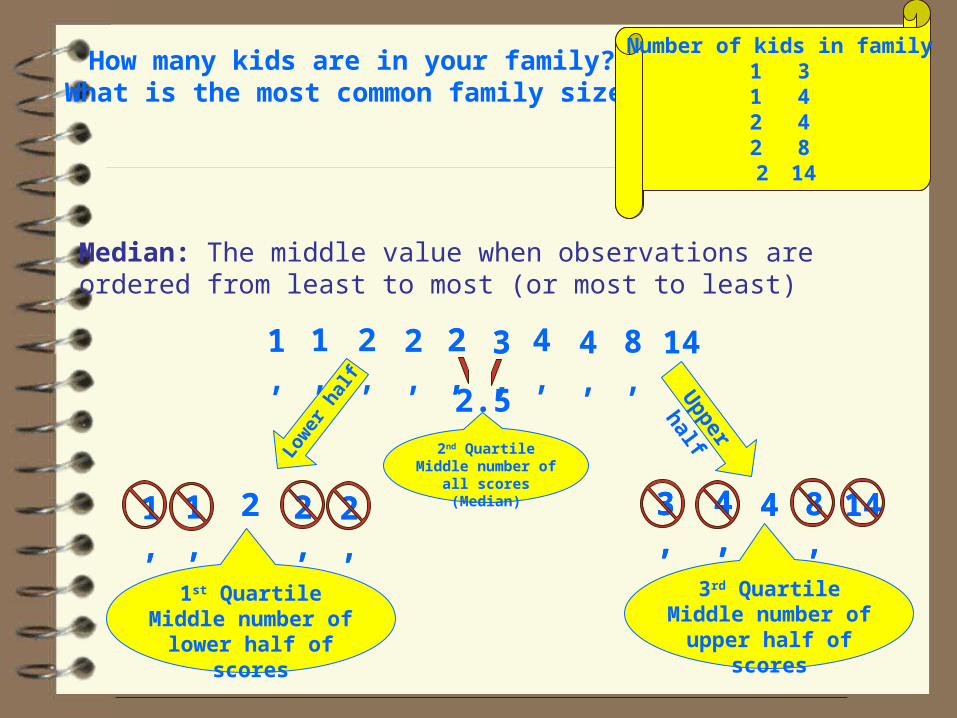
Median: The middle value when observations are ordered from least to most (or most to least)
How many kids are in your family?What is the most common family size?
Median: The middle value when observations are ordered from least to most (or most to least)
1, 3, 1, 4, 2, 4, 2, 8, 2, 14
1, 1, 2, 2, 2, 3, 4, 4, 8, 14
Number of kids in family1 43 21 84 2 2 14
Number of kids in family1 43 21 84 2 2 14
148,4,4,2,2,1,
How many kids are in your family?What is the most common family size?
Number of kids in family1 31 42 42 8 2 14
Median: The middle value when observations are ordered from least to most (or most to least)
1, 3, 1, 4, 2, 4, 2, 8, 2, 14
2.5
2, 3,1, 2, 4,2, 4, 8,1, 142, 3,1,
Median always has a percentile rank of 50% regardless of shape
of distribution
2 + 3 µ=2.5If there appears to be two
medians, take the mean of the twoMedian
also called the
2nd Quartile
4,
Number of kids in family1 43 21 84 2 2 14
148,4,4,2,2,1,
How many kids are in your family?What is the most common family size?
Number of kids in family1 31 42 42 8 2 14
2,1, 2, 4,2, 4, 8,1, 142,1,
148,4,4,2,2,1, 2, 3,1, 2, 3,
Median: The middle value when observations are ordered from least to most (or most to least)
1st QuartileMiddle number of lower half of
scores
Low
er h
alf
Upper
half
3rd QuartileMiddle number of upper half of
scores
3,3,3,
2.52nd Quartile
Middle number of all scores
(Median)

Mode: The value of the most frequent observation
Number of kids in family1 31 42 42 8 2 14
Score f .1 22 33 14 25 06 07 08 19 010 011 012 013 014 1
Please note:The mode is “2” because it is the most frequently occurring score.
It occurs “3” times. “3” is not the mode, it is
just the frequency for the value that is the
mode
Bimodal distribution: If there are two mostfrequent observations
What about central tendency for qualitative data?
Mode is good for nominal or ordinal data
Median can be used with ordinal data
Mean can be used with interval or ratio data
Overview Frequency distributions
The normal curve
Mean, Median,Mode, Trimmed Mean
Challenge yourself as we work through characteristics of distributions to try to categorize each concept as a measure
of 1) central tendency
2) dispersion or 3) shape
Skewed right, skewed leftunimodal, bimodal, symmetric