Lectures 3—4: Consumer Theory

Alexander Wolitzky

MIT

14.121

1

Consumer Theory

Consumer theory studies how rational consumer chooses what bundle of goods to consume.

Special case of general theory of choice.

Key new assumption: choice sets defined by prices of each of n goods, and income (or wealth).

2

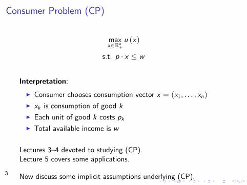
Consumer Problem (CP)

max u (x) x ∈Rn

+

s.t. p · x ≤ w

Interpretation:

� Consumer chooses consumption vector x = (x1, . . . , xn ) � xk is consumption of good k � Each unit of good k costs pk � Total available income is w

Lectures 3—4 devoted to studying (CP). Lecture 5 covers some applications.

Now discuss some implicit assumptions underlying (CP). 3

Prices are Linear

Each unit of good k costs the same.

No quantity discounts or supply constraints.

Consumer’s choice set (or budget set) is

B (p, w ) = {x ∈ Rn : p · x ≤ w }+

Set is defined by single line (or hyperplane): the budget line

p · x = w

Assume p ≥ 0.

4

Goods are Divisible

x ∈ Rn and consumer can consume any bundle in budget set +

Can model indivisibilities by assuming utility only depends on integer part of x .

5

Set of Goods is Finite

Debreu (1959):

A commodity is characterized by its physical properties, the date at which it will be available, and the location at which it will be available.

In practice, set of goods suggests itself naturally based on context.

6

Marshallian Demand

The solution to the (CP) is called the Marshallian demand (or Walrasian demand).

May be multiple solutions, so formal definition is:

Definition The Marshallian demand correspondence x : Rn × R � R+

n is+ defined by

x (p, w ) = argmax u (x)x ∈B (p,w ) = z ∈ B (p, w ) : u (z) = max u (x) .

x ∈B (p,w )

Start by deriving basic properties of budget sets and Marshallian demand.

7

Budget Sets Theorem Budget sets are homogeneneous of degree 0: that is, for all λ > 0, B (λp, λw ) = B (p, w ).

Proof.

B (λp, λw ) = {x ∈ Rn |λp · x ≤ λw }+

= {x ∈ Rn |p · x ≤ w } = B (p, w ) .+

Nothing changes if scale prices and income by same factor.

Theorem If p » 0, then B (p, w ) is compact.

Proof. For any p, B (p, w ) is closed. If p » 0, then B (p, w ) is also bounded.

8

Marshallian Demand: Existence

Theorem If u is continuous and p » 0, then (CP) has a solution. (That is, x (p, w ) is non-empty.)

Proof. A continuous function on a compact set attains its maximum.

9

Marshallian Demand: Homogeneity of Degree 0

Theorem For all λ > 0, x (λp, λw ) = x (p, w ).

Proof. B (λp, λw ) = B (p, w ), so (CP) with prices λp and income λw is same problem as (CP) with prices p and income w .

10

Marshallian Demand: Walras’Law

Theorem If preferences are locally non-satiated, then for every (p, w ) and every x ∈ (p, w ), we have p · x = w.

Proof. If p · x < w , then there exists ε > 0 such that Bε (x) ⊆ B (p, w ). By local non-satiation, for every ε > 0 there exists y ∈ Bε (x) such that y � x . Hence, there exists y ∈ B (p, w ) such that y � x . But then x ∈/ x (p, w ).

Walras’Law lets us rewrite (CP) as

max u (x) x ∈Rn

+

s.t. p · x = w 11

�

�

�

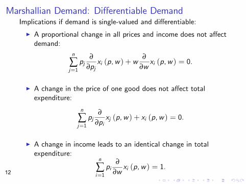
Marshallian Demand: Differentiable Demand Implications if demand is single-valued and differentiable:

A proportional change in all prices and income does not affect demand:

n ∂ ∂ pj xi (p, w ) + w xi (p, w ) = 0.

∂pj ∂w ∑ j =1

A change in the price of one good does not affect total expenditure:

n ∂ pj xj (p, w ) + xi (p, w ) = 0.

∂pi ∑ j =1

A change in income leads to an identical change in total expenditure:

n ∂ pi xi (p, w ) = 1.

∂w ∑ i =1

I

I

I

12

The Indirect Utility Function

Can learn more about set of solutions to (CP) (Marshallian demand) by relating to the value of (CP).

Value of (CP) = welfare of consumer facing prices p with income w .

The value function of (CP) is called the indirect utility function.

Definition The indirect utility function v : Rn × R → R is defined by +

v (p, w ) = max u (x) . x ∈B (p,w )

13

Indirect Utility Function: Properties

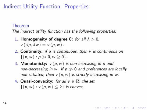
Theorem The indirect utility function has the following properties:

1. Homogeneity of degree 0: for all λ > 0, v (λp, λw ) = v (p, w ) .

2. Continuity: if u is continuous, then v is continuous on {(p, w ) : p » 0, w ≥ 0} .

3. Monotonicty: v (p, w ) is non-increasing in p and non-decreasing in w. If p » 0 and preferences are locally non-satiated, then v (p, w ) is strictly increasing in w.

4. Quasi-convexity: for all v̄ ∈ R, the set {(p, w ) : v (p, w ) ≤ v̄} is convex.

14

Indirect Utility Function: Derivatives

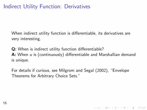
When indirect utility function is differentiable, its derivatives are very interesting.

Q: When is indirect utility function differentiable? A: When u is (continuously) differentiable and Marshallian demand is unique.

For details if curious, see Milgrom and Segal (2002), “Envelope Theorems for Arbitrary Choice Sets.”

15

Indirect Utility Function: Derivatives

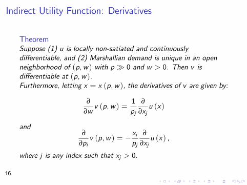
Theorem Suppose (1) u is locally non-satiated and continuously differentiable, and (2) Marshallian demand is unique in an open neighborhood of (p, w ) with p » 0 and w > 0. Then v is differentiable at (p, w ). Furthermore, letting x = x (p, w ), the derivatives of v are given by:

∂ 1 ∂ v (p, w ) = u (x)

∂w pj ∂xj

and ∂ xi ∂ v (p, w ) = − u (x) ,

∂pi pj ∂xj

where j is any index such that xj > 0.

16

�

�

�

�

�

Indirect Utility Function: Derivatives

∂ 1 ∂ ∂w v (p, w ) =

pj ∂xj u (x)

∂ ∂pi v (p, w ) = −

xi pj

∂ ∂xj u (x)

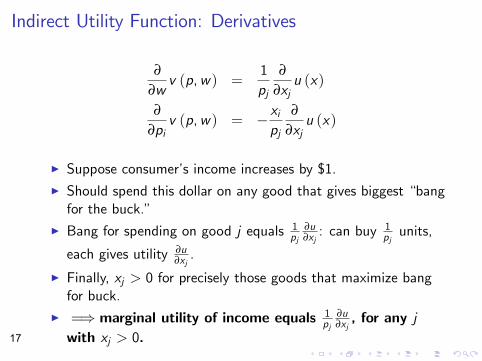
Suppose consumer’s income increases by $1.

Should spend this dollar on any good that gives biggest “bang for the buck.”

1 ∂u 1Bang for spending on good j equals : can buy units,pj ∂xj pj ∂ueach gives utility .∂xj

Finally, xj > 0 for precisely those goods that maximize bang for buck.

1 ∂u=⇒ marginal utility of income equals , for any jpj ∂xj with xj > 0.

I

I

I

I

I

17

�

�

�

�

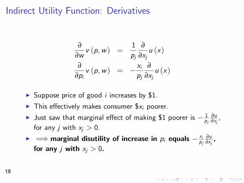
Indirect Utility Function: Derivatives

∂ 1 ∂ ∂w v (p, w ) =

pj ∂xj u (x)

∂ ∂pi v (p, w ) = −

xi pj

∂ ∂xj u (x)

Suppose price of good i increases by $1.

This effectively makes consumer $xi poorer. ∂uJust saw that marginal effect of making $1 poorer is − 1 ,pj ∂xj

for any j with xj > 0. ∂u=⇒ marginal disutility of increase in pi equals − xi ,pj ∂xj

for any j with xj > 0.

I

I

I

I

18

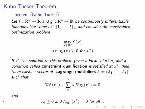
Kuhn-Tucker Theorem Theorem (Kuhn-Tucker) Let f : Rn → R and gi : Rn → R be continuously differentiable functions (for some i ∈ {1, . . . , I }), and consider the constrained optimization problem

max f (x) x ∈Rn

s.t. gi (x) ≥ 0 for all i

If x∗ is a solution to this problem (even a local solution) and a condition called constraint qualification is satisfied at x∗, then there exists a vector of Lagrange multipliers λ = (λ1, . . . , λI ) such that

Vf (x ∗ ) + I

∑ λi Vgi (x ∗ ) = 0 i =1

and λi ≥ 0 and λi gi (x ∗ ) = 0 for all i . 19

�

�

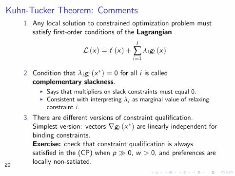
Kuhn-Tucker Theorem: Comments 1. Any local solution to constrained optimization problem must satisfy first-order conditions of the Lagrangian

I

L (x) = f (x) + ∑ λi gi (x) i =1

2. Condition that λi gi (x ∗) = 0 for all i is called complementary slackness.

Says that multipliers on slack constraints must equal 0. Consistent with interpreting λi as marginal value of relaxing constraint i .

3. There are different versions of constraint qualification. Simplest version: vectors Vgi (x ∗) are linearly independent for binding constraints. Exercise: check that constraint qualification is always satisfied in the (CP) when p » 0, w > 0, and preferences are locally non-satiated.

I

I

20

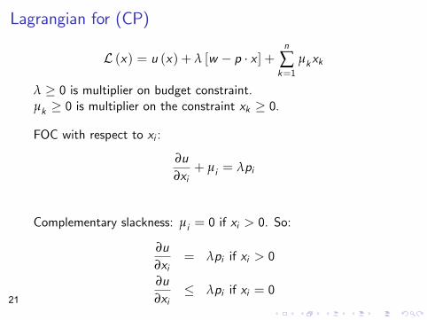
Lagrangian for (CP)

n

L (x) = u (x) + λ [w − p · x ] + ∑ µk xk k =1

λ ≥ 0 is multiplier on budget constraint. µk ≥ 0 is multiplier on the constraint xk ≥ 0.

FOC with respect to xi :

∂u + µi = λpi

∂xi

Complementary slackness: µi = 0 if xi > 0. So:

∂u = λpi if xi > 0

∂xi ∂u ≤ λpi if xi = 0 ∂xi 21

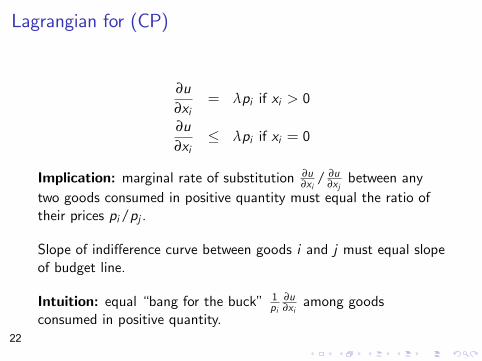
Lagrangian for (CP)

∂u = λpi if xi > 0

∂xi ∂u ≤ λpi if xi = 0 ∂xi

∂u / ∂uImplication: marginal rate of substitution between any ∂xi ∂xj two goods consumed in positive quantity must equal the ratio of their prices pi /pj .

Slope of indifference curve between goods i and j must equal slope of budget line.

∂uIntuition: equal “bang for the buck” 1 among goods pi ∂xi consumed in positive quantity.

22

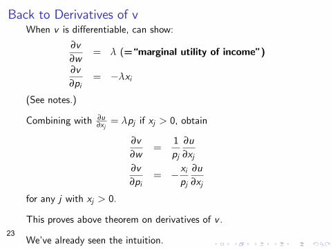
Back to Derivatives of v When v is differentiable, can show:

∂v = λ (=“marginal utility of income”)

∂w ∂v

= −λxi∂pi

(See notes.)

∂uCombining with ∂xj = λpj if xj > 0, obtain

∂v 1 ∂u =

∂w pj ∂xj ∂v

= − xi ∂u

∂pi pj ∂xj

for any j with xj > 0.

This proves above theorem on derivatives of v .

We’ve already seen the intuition. 23

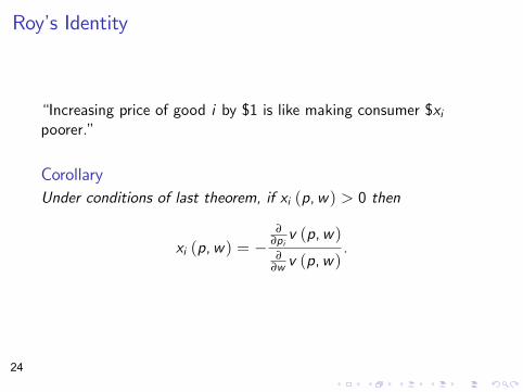
Roy’s Identity

“Increasing price of good i by $1 is like making consumer $xi poorer.”

Corollary Under conditions of last theorem, if xi (p, w ) > 0 then

∂ v (p, w )∂pixi (p, w ) = − . ∂ v (p, w )∂w

24

�

�

�

Key Facts about (CP), Assuming Differentiability

Consumer’s marginal utility of income equals multiplier on ∂vbudget constraint: = λ.∂w

Marginal disutility of increase in price of good i equals −λxi .

Marginal utility of consumption of any good consumed in positive quantity equals λpi .

I

I

I

25

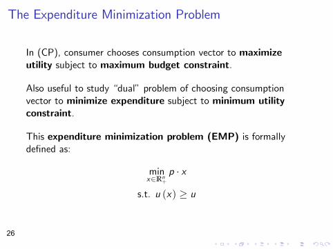
The Expenditure Minimization Problem

In (CP), consumer chooses consumption vector to maximize utility subject to maximum budget constraint.

Also useful to study “dual” problem of choosing consumption vector to minimize expenditure subject to minimum utility constraint.

This expenditure minimization problem (EMP) is formally defined as:

min p · x x ∈Rn

+

s.t. u (x) ≥ u

26

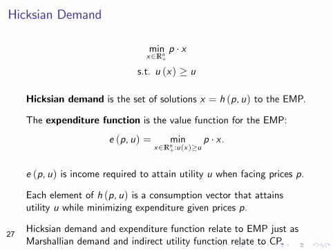
Hicksian Demand

min p · x x ∈Rn

+

s.t. u (x) ≥ u

Hicksian demand is the set of solutions x = h (p, u) to the EMP.

The expenditure function is the value function for the EMP:

e (p, u) = min p · x . x ∈Rn :u(x )≥u+

e (p, u) is income required to attain utility u when facing prices p.

Each element of h (p, u) is a consumption vector that attains utility u while minimizing expenditure given prices p.

Hicksian demand and expenditure function relate to EMP just as Marshallian demand and indirect utility function relate to CP.

27

Why Should we Care about the EMP?

For this course, 2 reasons:

(1) Hicksian demand useful for studying effects of price changes on “real” (Marshallian) demand.

In particular, Hicksian demand is key concept needed to decompose effect of a price change into income and substitution effects.

(2) Expenditure function important for welfare economics.

In particular, use expenditure function to analyze effects of price changes on consumer welfare.

28

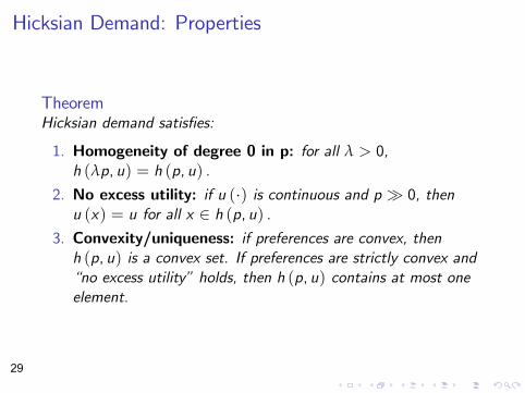
Hicksian Demand: Properties

Theorem Hicksian demand satisfies:

1. Homogeneity of degree 0 in p: for all λ > 0, h (λp, u) = h (p, u) .

2. No excess utility: if u (·) is continuous and p » 0, then u (x) = u for all x ∈ h (p, u) .

3. Convexity/uniqueness: if preferences are convex, then h (p, u) is a convex set. If preferences are strictly convex and “no excess utility” holds, then h (p, u) contains at most one element.

29

Expenditure Function: Properties

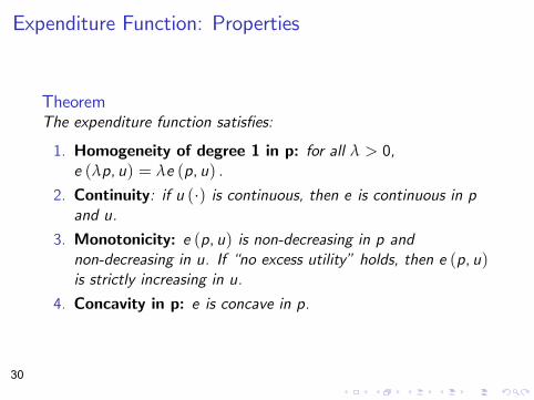
Theorem The expenditure function satisfies:

1. Homogeneity of degree 1 in p: for all λ > 0, e (λp, u) = λe (p, u) .

2. Continuity: if u (·) is continuous, then e is continuous in p and u.

3. Monotonicity: e (p, u) is non-decreasing in p and non-decreasing in u. If “no excess utility” holds, then e (p, u) is strictly increasing in u.

4. Concavity in p: e is concave in p.

30

Expenditure Function: Derivatives

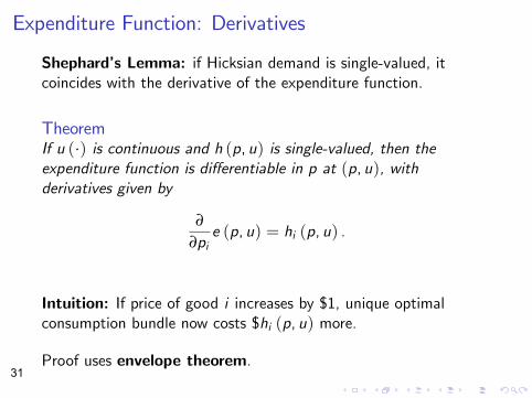
Shephard’s Lemma: if Hicksian demand is single-valued, it coincides with the derivative of the expenditure function.

Theorem If u (·) is continuous and h (p, u) is single-valued, then the expenditure function is differentiable in p at (p, u), with derivatives given by

∂ e (p, u) = hi (p, u) .

∂pi

Intuition: If price of good i increases by $1, unique optimal consumption bundle now costs $hi (p, u) more.

Proof uses envelope theorem. 31

Envelope Theorem

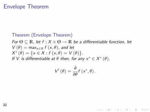
Theorem (Envelope Theorem) For Θ ⊆ R, let f : X × Θ → R be a differentiable function, let V (θ) = maxx ∈X f (x , θ), and let X ∗ (θ) = {x ∈ X : f (x , θ) = V (θ)}. If V is differentiable at θ then, for any x∗ ∈ X ∗ (θ),

∂ ∗V i (θ) = f (x , θ) . ∂θ

32

Shephard’s Lemma: Proof

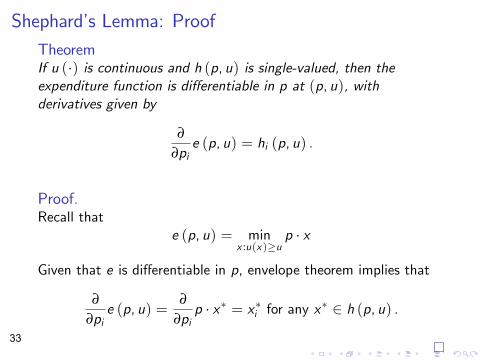
Theorem If u (·) is continuous and h (p, u) is single-valued, then the expenditure function is differentiable in p at (p, u), with derivatives given by

∂ e (p, u) = hi (p, u) .

∂pi

Proof. Recall that

e (p, u) = min p · x x :u(x )≥u

Given that e is differentiable in p, envelope theorem implies that

∂ ∂ ∗ ∗ ∗ e (p, u) = p · x = x for any x ∈ h (p, u) . ∂pi ∂pi

i

33

Comparative Statics

Comparative statics are statements about how the solution to a problem change with the parameters.

(CP): parameters are (p, w ), want to know how x (p, w ) and v (p, w ) vary with p and w .

(EMP): parameters are (p, u), want to know how h (p, u) and e (p, u) vary with p and u.

Turns out that comparative statics of (EMP) are very simple, and help us understand comparative statics of (CP).

34

The Law of Demand

“Hicksian demand is always decreasing in prices.”

Theorem (Law of Demand) iFor every p, pi ≥ 0, x ∈ h (p, u), and x i ∈ h (p , u), we have

pi − p x i − x ≤ 0.

Example: if pi and p only differ in price of good i , then i ipi − pi hi p , u − hi (p, u) ≤ 0.

Hicksian demand for a good is always decreasing in its own price.

Graphically, budget line gets steeper =⇒ shift along indifference curve to consume less of good 1. 35

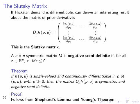
The Slutsky Matrix If Hicksian demand is differentiable, can derive an interesting result about the matrix of price-derivatives ⎛ ⎞

∂h1 (p,u) · · · ∂hn (p,u) ∂p1 ∂p1 . . .

. . . ∂h1 (p,u) · · · ∂hn (p,u)

∂pn ∂pn

⎜⎜⎝ ⎟⎟⎠Dph (p, u) =

This is the Slutsky matrix.

A n × n symmetric matrix M is negative semi-definite if, for all z ∈ Rn , z · Mz ≤ 0.

Theorem If h (p, u) is single-valued and continuously differentiable in p at (p, u), with p » 0, then the matrix Dph (p, u) is symmetric and negative semi-definite.

Proof. Follows from Shephard’s Lemma and Young’s Theorem. 36

The Slutsky Matrix

What’s economic content of symmetry and negative semi-definiteness of Slutsky matrix?

Negative semi-definiteness: differential version of law of demand.

Ex. if z = (0, . . . , 0, 1, 0, . . . , 0) with 1 in the j th component, then ∂hi (p,u)z · Dph (p, u) z = ∂pi

, so negative semi-definiteness implies

that ∂hi ∂(ppi

,u) ≤ 0.

Symmetry: derivative of Hicksian demand for good i with respect to price of good j equals derivative of Hicksian demand for good j with respect to price of good i .

Not true for Marshallian demand, due to income effects. 37

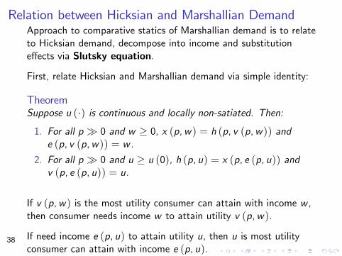
Relation between Hicksian and Marshallian Demand Approach to comparative statics of Marshallian demand is to relate to Hicksian demand, decompose into income and substitution effects via Slutsky equation.

First, relate Hicksian and Marshallian demand via simple identity:

Theorem Suppose u (·) is continuous and locally non-satiated. Then:

1. For all p » 0 and w ≥ 0, x (p, w ) = h (p, v (p, w )) and e (p, v (p, w )) = w.

2. For all p » 0 and u ≥ u (0), h (p, u) = x (p, e (p, u)) and v (p, e (p, u)) = u.

If v (p, w ) is the most utility consumer can attain with income w , then consumer needs income w to attain utility v (p, w ).

If need income e (p, u) to attain utility u, then u is most utility consumer can attain with income e (p, u).

38

�

�

�

��

�

, �

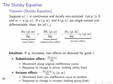
The Slutsky Equation Theorem (Slutsky Equation) Suppose u (·) is continuous and locally non-satiated. Let p » 0 and w = e (p, u). If x (p, w ) and h (p, u) are single-valued and differentiable, then, for all i , j ,

∂xi (p, w ) ∂hi (p, u) ∂xi (p, w ) = − xj (p, w ).

∂pj ∂pj ∂w , � , � income effect total effect substitution effect

Intuition: If pj increases, two effects on demand for good i : ∂hi (p,u)Substitution effect: ∂pj

Movement along original indifference curve. Response to change in prices, holding utility fixed.

Income effect: − ∂xi (p,w ) xj (p, w )∂w Movement from one indifference curve to another. Response to change in income, holding prices fixed.

I

I

I

II

I39

Terminology for Consumer Theory Comparative Statics

Definition Good i is a normal good if xi (p, w ) is increasing in w . It is an inferior good if xi (p, w ) is decreasing in w .

Definition Good i is a regular good if xi (p, w ) is decreasing in pi . It is a Giffen good if xi (p, w ) is increasing in pi .

Definition Good i is a substitute for good j if hi (p, u) is increasing in pj . It is a complement if hi (p, u) is decreasing in pj .

Definition Good i is a gross substitute for good j if xi (p, u) is increasing in pj . It is a gross complement if xi (p, u) is decreasing in pj . 40

�

�

�

�

�

�

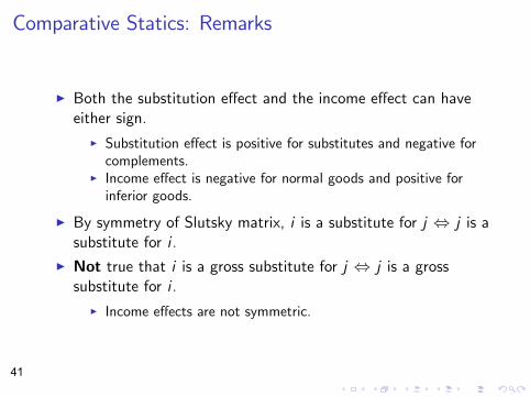
Comparative Statics: Remarks

Both the substitution effect and the income effect can have either sign.

Substitution effect is positive for substitutes and negative for complements. Income effect is negative for normal goods and positive for inferior goods.

By symmetry of Slutsky matrix, i is a substitute for j ⇔ j is a substitute for i .

Not true that i is a gross substitute for j ⇔ j is a gross substitute for i .

Income effects are not symmetric.

I

I

I

I

I

I

41

MIT OpenCourseWarehttp://ocw.mit.edu

14.121 Microeconomic Theory IFall 2015

For information about citing these materials or our Terms of Use, visit: http://ocw.mit.edu/terms.