L.G. Hill and R.L. Gustavsen- On the Characterization and Mechanisms of Shock Initiation in Heterogeneous Explosives

8/3/2019 L.G. Hill and R.L. Gustavsen- On the Characterization and Mechanisms of Shock Initiation in Heterogeneous Explosi…

http://slidepdf.com/reader/full/lg-hill-and-rl-gustavsen-on-the-characterization-and-mechanisms-of-shock 1/11

ON THE CHARACTERIZATION AND MECHANISMS OF SHOCK

INITIATION IN HETEROGENEOUS EXPLOSIVES

L.G. Hill and R.L. GustavsenLos Alamos National Laboratory

Los Alamos, NM 87545

We present a new methodology for fitting x-t shock initiation data based upon extended detonation shock dynamics (DSD) theory.Fits are generated by simple, analytic phase plane functions. Wedemonstrate the technique using recent PBX 9501 and PBX 9502gas gun data. The method enhances Pop plot and inert Hugoniotaccuracy, and provides extended DSD calibration in the initiationregime. It is also useful for studying physical initiation mechan-isms. We use it to evaluate the single curve initiation model. We

then develop an approximately universal fitting function for reaction build-up, from which the c-j reaction zone thickness can be estimated. Finally, we define a practical figure-of-merit toquantify homogeneous/heterogeneous initiation character.

INTRODUCTION

At the time of this writing the shock initiationwedge test has been in use for over 40 years.Data analysis methods have changed little sincethe first classic studies in 1960.1,2 Most oftenone draws a line through the early (approximate-

ly inert) x-t shock data, and a second line throughthe late (steadily detonating) data. An inertHugoniot point is inferred, in part, from the slopeof the first line. Detonation transition is taken asthe point (t*, x*) where the two lines cross.Transition has also been defined as the point onthe shock record where the slope first differs per-ceptibly from that of the steady detonation.Often, methods have been based upon featuresthat can be read directly from the film record.

The problems with traditional methods are that

they 1) do not use any definite or repeatable physical criterion, 2) differ in implementation between experimenters, 3) do not use all therecord information, 4) have certain systematicerrors, and 5) do not take advantage of recenttheoretical and computational advances.

Historically, wedge test analysis errors have been eclipsed by experimental ones, the foremost being 1) limited planarity of the plane wave lens,and 2) imperfect and variable pressure support provided by the following flow. Consequently

the end result has been somewhat forgiving of analytical approach. Recent refinements in gasgun experimental techniques3 have substantiallyreduced the two primary sources of experimentalerror. Better analysis methods will allow thisnew class of data to realize its full potential.

The method we explore is motivated byextended detonation shock dynamics (DSD)theory4. DSD suggests a class of smooth gener-ating functions of the form a[U ], where U is theshock speed and a is its acceleration. Fits gener-

ated in this manner can fit x-t data in fine detail,thereby expanding its usefulness. First, it helpsus to more accurately determine inert Hugoniotand Pop plot curves. Secondly, it allows one tocalibrate the extended DSD model in a region far from that covered by current experiments.



Beyond the utilitarian objectives of character-ization and calibration, accurate shock trajectoryfits can help deduce physical initiation mech-anisms. Shock trajectories, together with mag-netic particle velocity records, comprise the primary information available for appraisingreaction rate models in the initiation regime.

A question that is closely related to reactionrate laws is how well initiation follows the popular single curve initiation (SCI) model, uponwhich the Forest Fire reaction rate form5 is built.SCI is appealing for its utility; however, it haslittle theoretical motivation to recommend it, andthere is disagreement as to how well it works andunder what conditions. Accurate shock traj-ectories can help answer this question.

Another important issue is how various explo-sives differ as to the nature of their build up to

detonation—what has been loosely referred to asthe relative degree of “heterogeneity” versus“homogeneity”. To date, descriptions have beenmostly qualitiative. With sufficiently accurateshock trajectory fits, one is in a position toquantify some of these concepts.

THEORETICAL FOUNDATION Our approach is based upon recent extensions todetonation shock dynamics (DSD) theory, thecurrent status of which are addressed elsewherein these proceedings.4 We give only a brief

summary here to motivate the connection.DSD is an approximation to the reactive Euler

equations that allows numerically efficienttracking of curved detonation waves. Fullnumerical simulation involves calculating thereaction zone structure, for which one mustspecify both the “mixture” equation-of-state(EOS) and the reaction rate for the burningexplosive. This is doubly problematic because a)the mixture EOS and the reaction rate are poorlyknown, and b) calculating the reaction zone isvery computationally intensive.

DSD avoids both problems through the use of an intrinsic relation, which is a theoreticallymotivated mathematical expression relating thelocal wave shape to its local motion. The intrins-

ic relation coefficients for a given HE dependupon both its EOS and reaction rate; however, noexplicit knowledge of the two is necessary.Rather, the intrinsic relation is calibrated directlyfrom suitable detonation experiments.6

A convex detonation shock is causally insulat-ed from the downstream world by a sonic

surface. This attribute makes an intrinsic relation(which knows only about conditions at the shock front, and nothing of downstream world) math-ematically well-posed. An initiating shock lacksthis condition over much of its run-up, and isgenerally driven by both reactive heat release and back boundary motion. The extreme case is thatof an inert shock, which is driven entirely by back boundary motion. Here Whitham’s shock dynamic theory7 (the predecessor to DSD) isnevertheless a useful approximation in many

cases.DSD is actually a hierarchy of models ordered by the complexity of the intrinsic relation. Thezeroth approximation is Huygens’ construction.In the first approximation κ, the total local shock curvature, depends upon Dn, the correspondingnormal velocity component. Any model using ahigher-order intrinsic relation (involving tempor-al and spatial derivatives of κ and Dn) has beencalled an extended model.

In the simplest extended models, the intrinsic

relation for κ = 0 (a plane wave) relates Dn to theshock acceleration d Dn/dt —which amounts to asimple model for shock initiation. The assump-tion that this acceleration function is the samefor all shock inputs is equivalent to the SCImodel. Thus one could say that extended DSDhas a Forest Fire-like initiation model.

In their extensive paper on extended DSDtheory, Yao and Stewart8 compute a theoreticalintrinsic relation assuming an ideal gas EOS, and

Arrhenius kinetics with high activation energy.When applied to a plane wave (κ = 0), a simpli-fied version of the Yao-Stewart equation (inwhich higher order terms are neglected) providesa good launching point for applying the extendedDSD to shock initiation.



THE ACCELERATION FUNCTION

In the (κ, Dn, d Dn/dt ) level of the extendedtheory, with set to zero, the Yao-Stewart (Y-S)intrinsic relation reduces to the expression

a

am

= D −U

D −U m

exp

U −U m D −U m

. (1)

We adopt a slightly different notation than isused in the DSD literature, one that is descriptiveof this particular problem. We denote the shock velocity by U , the shock acceleration by a, andthe steady Chapman-Jouguet (c-j) velocity by D.Generally D is a fitting parameter, but it may bespecified as a constraint if it is sufficiently wellknown from rate stick experiments. The other two fitting parameters are likewise chosen tohave physical significance: am is the peak ac-celeration; U m is the velocity at which it occurs.

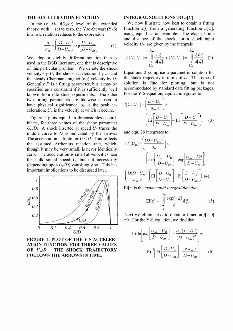
Figure 1 plots eqn. 1 in dimensionless coord-inates, for three values of the shape parameter U m/ D. A shock inserted at speed U 0 traces themiddle curve to D as indicated by the arrows.The acceleration is finite for U < D. This reflectsthe assumed Arrhenius reaction rate, which,though it may be very small, is never identicallyzero. The acceleration is small at velocities near the bulk sound speed C , but not necessarily(depending upon U m/ D) vanishingly so. This hasimportant implications to be discussed later.

FIGURE 1: PLOT OF THE Y-S ACCELER-

ATION FUNCTION, FOR THREE VALUES

OF U m/ D. THE SHOCK TRAJECTORY

FOLLOWS THE ARROWS IN TIME.

INTEGRAL SOLUTIONS TO a[U ] We now illustrate how best to obtain a fitting

function x[t ] from a generating function a[U ],using eqn. 1 as an example. The elapsed timeand distance of the shock, for a shock inputvelocity U 0, are given by the integrals

t [U ; U 0 ] =dξ

a[ξ ]U 0

U

∫ ; x [U ; U 0 ] =ξ dξ

a[ξ ]U 0

U

∫ . (2)

Equations 2 comprise a parametric solution for the shock trajectory in terms of U . This type of solution is fine for plotting, but is notaccommodated by standard data fitting packages.For the Y-S equation, eqn. 2a integrates to:

t [U ; U 0 ] = D − U m

am e

×

Ei D − U 0

D − U m

− Ei D − U

D − U m

, (3)

and eqn. 2b integrates to:

x *[U 0] =( D −U m )2

am

×

expU m −U 0 D −U m

− exp

U m − Ud

D −U m

+

D( D −U m )am e

Ei D −U 0

D −U m

− Ei D −U d

D −U m

. (4)

Ei[ z ] is the exponential integral function,

Ei[ z ] =exp[−ξ ]

ξ -z

∞

∫ dξ . (5)

Next we eliminate U to obtain a function f [ x, t ]=0. For the Y-S equation, we find that

1+ ln exp U m − U 0 D − U m

− am ( x − D t )

( D − U m )2

=

Ei−1

Ei D -U 0

D -U m

−

e am t

D − U m

. (6)



The final step is to solve for t [ x] or x[t ], either of which can be used to directly fit data. For Y-S,

x[ t ; U 0 ] = D t −( D − U m )2

am

× (7)

exp D −U 0 D −U m

− exp Ei−1 Ei

D −U 0 D −U m

−

am t D −U m

One finds that these three steps can be per-formed only for certain simple expressions for a[U ]. In some cases only the first step is possible, and in others two out of three. When afull analytic solution is possible, it is often interms of special functions and their inverses, as isthe case for eqn. 1. This poses no problem, solong as all functions are known to the computingenvironment. Otherwise, they must be defined.

For equations allowing a subset of the abovesolution steps, or if undefined special functionsare generated, then it is generally easiest tonumerically compute the desired solution directlyfrom a[U ]. For example, to compute x[t ] onewould solve the following second order ODE:

ÝÝ x[t ] = a Ý x[t ][ ]; x[0] = 0; Ý x[0] = U 0 , (8)

which modern mathematics packages will solvealmost instantly by a single command. Withmodest effort, one may manually input trial parameters and iterate to achieve a good fit.Otherwise, a least squares analysis will generallyrequire some programming. In our case weconstructed a simple Mathematica

® fitting algo-rithm based on eqn. 8.

SINGLE CURVE INITIATION MODEL The single curve initiation model (SCI)

assumes that all shock trajectories follow thesame “master build-up” curve. The idea is mostfrequently expressed in the x-t plane, where alltrajectories centered on (t *, x*) are identical

regardless of U 0. The x-t master curve can betransformed to other planes, for example a[U ],U [t ], and U [ x]. In fact we shall find these planes(and particularly a[U ]) more useful in appraisingthe SCI model than x-t , which turns out to be tooinsensitive a measure.

If formal SCI assumption is simple, the physi-cal implications are less obvious. The simplethought experiment illustrated in Fig. 4 isilluminating. In Fig. 4a, an explosive sample isimpacted by a flyer-plate of velocity u1, whichgenerates a shock of velocity U 1. After a time t the shock has accelerated, due to reaction in theshocked material, to a greater speed U 2 (Fig. 4b).

In Fig. 4c an identical sample is shocked by aflyer of speed u2, to an initial speed U 2. SCIassumes that cases 4b) and 4c) behave identically as the shock accelerates from U 2 to D, for all possible combinations of u1 and t . This canonly happen if the shock in 4b) is unaffected bythe additional layer of reacting material. This inturn implies that reaction is concentrated near theshock front (as for the steady detonation), or thata sonic surface promptly develops that insulatesthe shock from the downstream reacting material.

Consequently short and sustained shocks behavethe same in the SCI model.

FIGURE 2: THOUGHT EXPERIMENT TO

ILLUSTRATE SCI MODEL PROPERTIES.

The SCI picture does not mesh well with our physical understanding of the initiation process.In fact, the initiation of a physically homo-geneous explosive is thought to be much theopposite situation. In that case the shockedexplosive self-heats, or “cooks”, for an induction

time ∆t before reaction runs away. Thermalexplosion then begins near the back boundarywhere material has cooked the longest. Aninduction locus then advances according to alighting-time schedule set by the input shock.The prescription is that the induction locus



follows the shock at the same speed U 0, adistance U 0 ∆t behind. Soon heat release coupleswith the mechanics, transforming the thermaldisturbance into a pressure wave that overtakesthe shock. For sufficiently large U 0 ∆t thesecondary wave will itself steepen into a shock,and will upon overtake impulsively acceleratethe lead wave past the c-j velocity, which thelatter then approaches asymptotically fromabove. Generally initiation is said to be “homo-geneous” if the shock velocity overshoots, and“heterogeneous” otherwise.

In contrast, heterogeneous explosives initiateonly by the aid of energy localization and “hotspots”. When a hot region is created in a shock-ed PBX, there is a brief moment of competition between heat generation and loss. If reactionwins it does so quickly. This is a step toward theideal SCI behavior outlined in Fig. 4. On theother hand, reaction does not necessary finish quickly, as hot spot initiated-reaction must fill into consume the surrounding material.

Measured PBX initiation behavior is basicallyconsistent with this generic reasoning about hotspots. PBX’s do not exhibit overshoot, whichimplies that any overtaking disturbance isdiffuse. This conclusion is supported by mag-netic particle velocity gauges, which show that a broad “hump” of reacting flow develops that

grows, sharpens, and moves forward to catch theshock. Ultimately it evolves into the steadyreaction zone structure.

THE KINEMATIC SCI POP PLOT

One nice feature of the SCI model is that theU [t ] and U [ x] master curves can be transformedto kinematic Pop plots, a term we’ve coined for t *[U 0] or x*[U 0]. (One can easily transform tothe traditional dynamic Pop plot, t *[ P 0] or x*[ P 0],if the inert Hugoniot is known.) In principle, onecan estimate the kinematic Pop plot from a single

initiation record or, conversely, calculate shock trajectories from the Pop-plot.

The transformation from the laboratory to thePop plot frame is illustrated in Fig. 5. For everyvalue of the input shock velocity U 0 there is atransition point x*, defined by some initiationcriterion U = U d , which also lies on the master curve. The locus of all possible (U 0, x*) pairstherefore map out the master curve. We needonly change our coordinate system to adopt thePop plot interpretation. The new coordinatesystem is shown in Fig. 5a, and the completedtransformation is shown in Fig. 5b. If t [U ] =f[U ], then the transformation rule is t *[U 0] =f[U d ] – f[U 0]. Likewise if If x[U ] = g[U ], thenthe transformation rule is x*[U 0] = g[U d ] – g[U 0].For the Y-S equation the kinematic Pop plott *[U 0] is given by:

t *[U 0] = D −U m

e am

×

Ei D −U 0 D −U m

− Ei D −U d D −U m

. (9)

A) SCI VELOCITY MASTER CURVE B) KINEMATIC SCI POP PLOT

FIGURE 3. TRANSFORMATION FROM THE VELOCITY MASTER CURVE TO THE

KINEMATIC SCI POP PLOT. THE COORDINATES ARE LINEAR.



Likewise, the result for x*[U 0] is

x *[U 0] =( D −U m )2

am

× (10)

expU m −U 0 D −U m

− exp

U m −U d

D −U m

+

D( D −U m )am e

Ei D −U 0

D −U m

− Ei D −U d

D −U m

.

The definition of the threshold U d is a matter of preference. U d = U m and U d = η D are bothobvious choices. The first definition is aesthetic because it has no arbitrary parameters; thesecond is attractive because for fixed D, theupper Pop plot termination does not depend uponthe fitting parameters.

FITS TO PBX 9501 AND PBX 9502 DATAWe now fit eqn. 1 to recent PBX 9501 and

PBX 9502 gas gun data. Existing shots for eachexplosive were designed to generate three nom-inal input pressures that resulted in short,medium, and long runs in the fixed samplelength. We have selected the nicest data set ineach of the six categories for detailed study.

In fitting each HE, we begin by assuming thatSCI holds. That is, we jointly fit the threerecords to a common a[U ] by keeping the

parameters U m and am the same for all sets. U 0 isof course different for each sample. D wasconstrained to 8.80 mm/µs for PBX 9501 and7.65 mm/µs for PBX 9502. (The true c-j

velocity for PBX 9502 is poorly known due to anupturn in the diameter effect curve as 1/ R -> 0.Values as high as 7.8 mm/µs have been extra- polated; the present value is that which best fitsthe current data.) We also allowed a separateoffset X 0 for each record, as the magnetic gaugeshad a placement tolerance of roughly 100 µmwithin the sample. Best-fit values greater thanabout 100 µm were considered suspicious, buttypically the calculated offsets were of this order or less.

To test for departure from SCI, we performed asecond series of fits in which U m and am wereallowed separate values for each record. The best-fit parameters from the first (SCI) fit wereused as starting values for the individual fits.This two-step procedure helped to ensure that thedifferent records didn’t get trapped in different

local minima of the merit function.The three PBX 9501 data sets are plotted inFig. 2. The x-t points were generated by mag-netic shock tracker gauges, which are describedelsewhere in these proceedings.3 The individualfits to the data are superimposed, and the fitquality is excellent in all three cases. Thestandard deviation of the fit residuals σ (mag-nified 10x in the plots) were 17, 27, and 16 µmrespectively. The three PBX 9502 data sets are plotted in Fig. 3. There were multiple gauge

packages in these shots, and a small interleavingerror is apparent in the fit residual pattern. Thisincreased the σ’s (which were 37, 43, and 45 µmrespectively) relative to the PBX 9501.

A) SHORT RUN (#1154) B) MEDIUM RUN (#1179) C) LONG RUN (#1165)

FIGURE 4: INDIVIDUAL FITS TO THREE PBX 9501 SHOCK INITIATION DATA SETS.



A) SHORT RUN (#2s-85) B) MEDIUM RUN (#2s-86) C) LONG RUN (#2s-70)

FIGURE 5: INDIVIDUAL FITS TO THREE PBX 9502 SHOCK INITIATION DATA SETS.

Figure 6 plots a[U ] corresponding to the fits of Figs. 4 and 5. For both HE’s the functions areordered according to U 0 or, alternatively, x*.This is compelling evidence that build-up doesnot strictly follow the SCI model. Moreover, thedeparture is sensible based on the previousdiscussion: weaker inputs and longer runs allow

the reacting flow more time and distance toorganize and steepen into an overtaking wave.

There are perhaps two reasons why we detectSCI breakdown where most previous studieshave not. The first is improved data quality; thesecond is that a[U] is a sensitive plane. In fact,the differences it exposes may be too sensitive toaffect many engineering calculations. To testthis aspect we compared the quality of x-t fits for individual records (i.e., Figs. 4 and 5), to thoseobtained under SCI-constraint. The medium-run

fits were virtually unchanged, since the SCI fitsreflect the average behavior of the sets. Theshort and long-run fits were still very good. The

SCI σ’s were 26, 27, and 20 µm for PBX 9501 (a22% average increase) and 38, 43, and 47 µm for PBX 9502 (a 2.4% average increase). Thesmaller increase for 9502 is likely due to theuncertainty introduced by gauge interleaving.

We have noted that eqn. 1 has finite acceler-ation for all U < D. This means that an acousticwave eventually runs to detonation—even for PBX 9502! In reality, a PBX subjected to aweak shock relies on the hot spot mechanism toinitiate reaction. That process is completelyabsent for acoustic waves, and for elastic wavesas well. Hot spots form only when the shockedstress level exceeds the material strength, suchthat the initially heterogeneous compact homo-genizes in a manner that produces localizedenergy dissipation. Evidently, initiation cannotoccur below U h, the shock velocity at the Hugoniot elastic limit . The distinction has littleeffect on the present model, as Fig. 6 shows thatU h and C are nearly equivalent9,10.

A) PBX 9501 B) PBX 9502

FIGURE 6: ACCELERATION FUNCTIONS FOR THE X-T FITS OF FIGS. 4 AND 5.



On Inert Hugoniot Accuracy

The inert Hugoniot curve is constructed from acollection of (u0, U 0) data pairs. U 0 is the initialshock velocity, a fitting parameter in thisanalysis. u0 is the input particle velocity, whichfor a traditional wedge test is inferred by animpedance-matching calculation. One gets asingle Hugoniot point per traditional wedge test.

Whether the data comes from a firing site or agas gun, the traditional method for inferring U 0 isto fit a straight line to the early shock trajectory.Since the goal is to construct an inert Hugoniot,one wishes to obtain the measurement over ashort time and distance, before reaction accel-erates the shock and spoils the result. The di-lemma is that measurements over short times anddistances lead to large uncertainties in the slope.

Fitting a straight line to an accelerating curveleads to an overestimate of the initial slope U 0.From the shape of a[U ] it is clear that the effect becomes progressively worse as U 0 increases.The present method computes the local value of U 0 from a fit that follows the general trend. Asexpected, this method gives consistently smaller,and presumably more accurate, values for U 0 than does the traditional straight-line method.

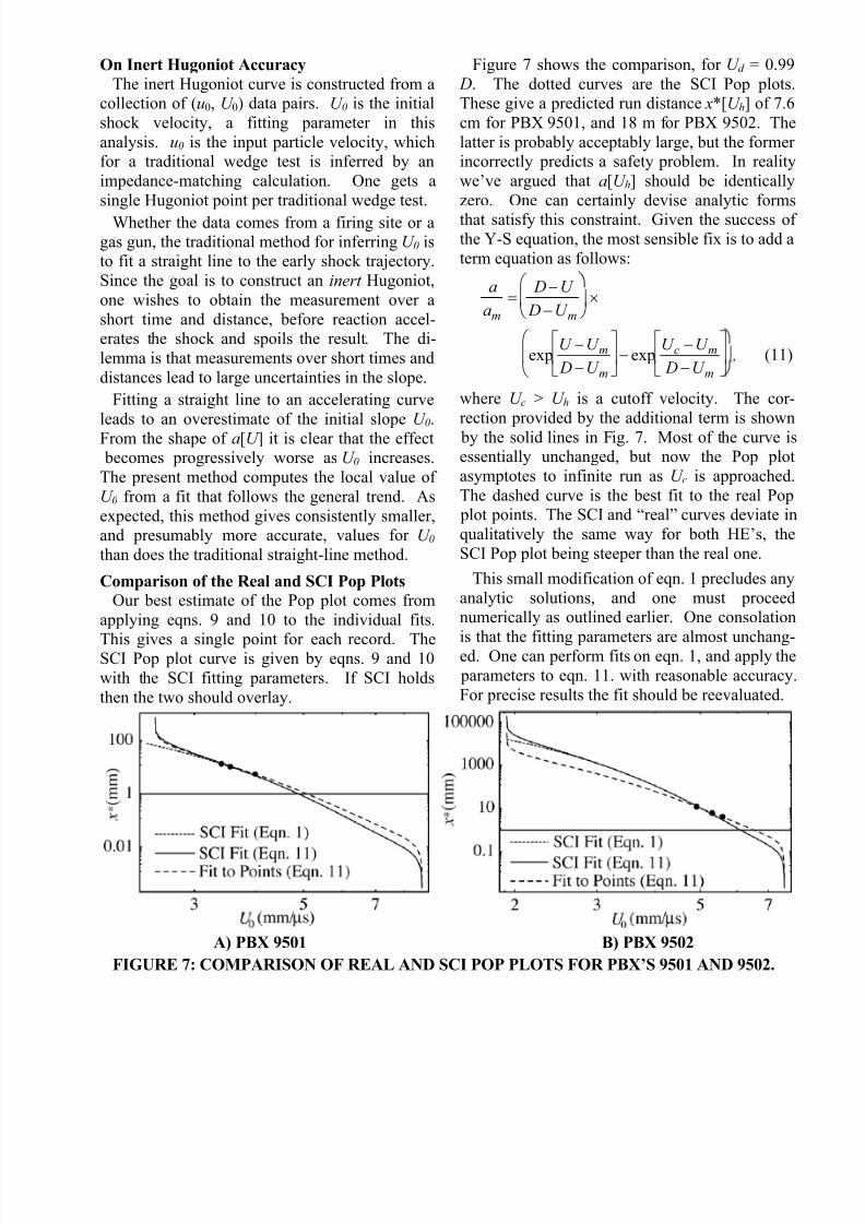
Comparison of the Real and SCI Pop Plots Our best estimate of the Pop plot comes from

applying eqns. 9 and 10 to the individual fits.

This gives a single point for each record. TheSCI Pop plot curve is given by eqns. 9 and 10with the SCI fitting parameters. If SCI holdsthen the two should overlay.

Figure 7 shows the comparison, for U d = 0.99 D. The dotted curves are the SCI Pop plots.These give a predicted run distance x*[U h] of 7.6cm for PBX 9501, and 18 m for PBX 9502. Thelatter is probably acceptably large, but the former incorrectly predicts a safety problem. In realitywe’ve argued that a[U h] should be identicallyzero. One can certainly devise analytic forms

that satisfy this constraint. Given the success of the Y-S equation, the most sensible fix is to add aterm equation as follows:

a

am

= D −U

D −U m

×

expU −U m D −U m

− exp

U c −U m D −U m

, (11)

where U c > U h is a cutoff velocity. The cor-rection provided by the additional term is shown by the solid lines in Fig. 7. Most of the curve isessentially unchanged, but now the Pop plotasymptotes to infinite run as U c is approached.The dashed curve is the best fit to the real Pop plot points. The SCI and “real” curves deviate inqualitatively the same way for both HE’s, theSCI Pop plot being steeper than the real one.

This small modification of eqn. 1 precludes anyanalytic solutions, and one must proceednumerically as outlined earlier. One consolation

is that the fitting parameters are almost unchang-ed. One can perform fits on eqn. 1, and apply the parameters to eqn. 11. with reasonable accuracy.For precise results the fit should be reevaluated.

A) PBX 9501 B) PBX 9502

FIGURE 7: COMPARISON OF REAL AND SCI POP PLOTS FOR PBX’S 9501 AND 9502.



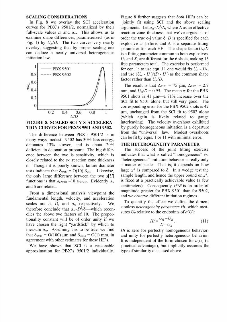
SCALING CONSIDERATIONS

In Fig. 8 we overlay the SCI accelerationcurves for PBX’s 9501/2, normalized by their full-scale values D and am. This allows us toexamine shape differences, parameterized (as inFig. 1) by U m/ D. The two curves very nearlyoverlay, suggesting that by proper scaling onecan deduce a nearly universal heterogeneous

initiation law.

FIGURE 8. SCALED SCI Y-S ACCELERA-

TION CURVES FOR PBX’S 9501 AND 9502.

The difference between PBX’s 9501/2 is inmany ways modest. 9502 has 30% less energy,detonates 13% slower, and is about 20%deficient in detonation pressure. The big differ-ence between the two is sensitivity, which isclosely related to the c-j reaction zone thicknessδ. Though it is poorly known, failure diameter

tests indicate that δ9502 = O(10) δ9501. Likewise,the only large difference between the two a[U ]functions is that am9501 ~10 am9502. Evidently am and δ are related.

From a dimensional analysis viewpoint thefundamental length, velocity, and accelerationscales are δ, D, and am respectively. Wetherefore conclude that am~ D2/δ —which recon-ciles the above two factors of 10. The propor-tionality constant will be of order unity if we

have chosen the right “yardstick” by which tomeasure am. Assuming this to be true, we findthat δ9501 = O(100) µm and δ9502 = O(1) mm, inagreement with other estimates for these HE’s.

We have shown that SCI is a reasonableapproximation for PBX’s 9501/2 individually.

Figure 8 further suggests that both HE’s can be jointly fit using SCI and the above scalingarguments. Let am= D2/∆, where ∆ as an effectivereaction zone thickness that we’ve argued is of order the true c-j value δ. D is specified for eachexplosive as before, and ∆ is a separate fitting parameter for each HE. The shape factor U m/ D is a fitting parameter common to both explosives.U 0 and X 0 are different for the 6 shots, making 15free parameters total. The exercise is performedfor eqn. 1; to use eqn. 11 one would fix U c ~ U h,and use (U m - U c)/( D - U c) as the common shapefactor rather than U m/ D.

The result is that ∆9501 = 75 µm, ∆9502 = 2.7mm, and U m/ D = 0.95. The mean σ for the PBX9501 shots is 41 µm—a 71% increase over theSCI fit to 9501 alone, but still very good. Thecorresponding error for the PBX 9502 shots is 42

µm, unchanged from the SCI fit to 9502 alone(which again is likely related to gaugeinterleaving). The velocity overshoot exhibited by purely homogeneous initiation is a departurefrom the “universal” law. Modest overshootscan be fit by eqns. 1 or 11 with minimal error.

THE HETEROGENEITY PARAMETER

The success of the joint fitting exerciseindicates that what is called “homogeneous” vs.“heterogeneous” initiation behavior is really onlya matter of scale. That is, it depends on how

large x* is compared to δ. In a wedge test thesample length, and hence the upper bound on x*,is fixed at a practically achievable value (a fewcentimeters). Consequently x*/δ is an order of magnitude greater for PBX 9501 than for 9502,and we observe different initiation regimes.

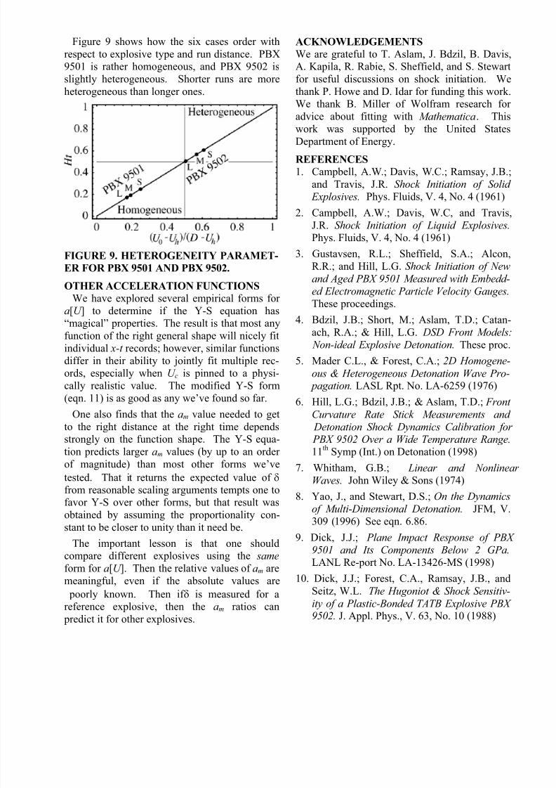
To quantify the effect we define the dimen-sionless heterogeneity parameter Ht , which mea-sures U 0 relative to the endpoints of a[U ]:

Ht ≡U 0 −U h

D −U h

. (11)

Ht is zero for perfectly homogeneous behavior,and unity for perfectly heterogeneous behavior.It is independent of the form chosen for a[U ] (a practical advantage), but implicitly assumes thetype of similarity discussed above.



Figure 9 shows how the six cases order withrespect to explosive type and run distance. PBX9501 is rather homogeneous, and PBX 9502 isslightly heterogeneous. Shorter runs are moreheterogeneous than longer ones.

FIGURE 9. HETEROGENEITY PARAMET-

ER FOR PBX 9501 AND PBX 9502.

OTHER ACCELERATION FUNCTIONS

We have explored several empirical forms for a[U ] to determine if the Y-S equation has“magical” properties. The result is that most anyfunction of the right general shape will nicely fitindividual x-t records; however, similar functionsdiffer in their ability to jointly fit multiple rec-ords, especially when U c is pinned to a physi-cally realistic value. The modified Y-S form(eqn. 11) is as good as any we’ve found so far.

One also finds that the am value needed to getto the right distance at the right time dependsstrongly on the function shape. The Y-S equa-tion predicts larger am values (by up to an order of magnitude) than most other forms we’vetested. That it returns the expected value of δ from reasonable scaling arguments tempts one tofavor Y-S over other forms, but that result wasobtained by assuming the proportionality con-stant to be closer to unity than it need be.

The important lesson is that one should

compare different explosives using the same form for a[U ]. Then the relative values of am aremeaningful, even if the absolute values are poorly known. Then if δ is measured for areference explosive, then the am ratios can predict it for other explosives.

ACKNOWLEDGEMENTS

We are grateful to T. Aslam, J. Bdzil, B. Davis,A. Kapila, R. Rabie, S. Sheffield, and S. Stewartfor useful discussions on shock initiation. Wethank P. Howe and D. Idar for funding this work.We thank B. Miller of Wolfram research for advice about fitting with Mathematica. Thiswork was supported by the United States

Department of Energy.REFERENCES

1. Campbell, A.W.; Davis, W.C.; Ramsay, J.B.;and Travis, J.R. Shock Initiation of Solid Explosives. Phys. Fluids, V. 4, No. 4 (1961)

2. Campbell, A.W.; Davis, W.C, and Travis,J.R. Shock Initiation of Liquid Explosives. Phys. Fluids, V. 4, No. 4 (1961)

3. Gustavsen, R.L.; Sheffield, S.A.; Alcon,R.R.; and Hill, L.G. Shock Initiation of New

and Aged PBX 9501 Measured with Embedd-ed Electromagnetic Particle Velocity Gauges.These proceedings.

4. Bdzil, J.B.; Short, M.; Aslam, T.D.; Catan-ach, R.A.; & Hill, L.G. DSD Front Models: Non-ideal Explosive Detonation. These proc.

5. Mader C.L., & Forest, C.A.; 2D Homogene-

ous & Heterogeneous Detonation Wave Pro- pagation. LASL Rpt. No. LA-6259 (1976)

6. Hill, L.G.; Bdzil, J.B.; & Aslam, T.D.; Front

Curvature Rate Stick Measurements and Detonation Shock Dynamics Calibration for PBX 9502 Over a Wide Temperature Range.11th Symp (Int.) on Detonation (1998)

7. Whitham, G.B.; Linear and Nonlinear Waves. John Wiley & Sons (1974)

8. Yao, J., and Stewart, D.S.; On the Dynamicsof Multi-Dimensional Detonation. JFM, V.309 (1996) See eqn. 6.86.

9. Dick, J.J.; Plane Impact Response of PBX

9501 and Its Components Below 2 GPa.LANL Re-port No. LA-13426-MS (1998)

10. Dick, J.J.; Forest, C.A., Ramsay, J.B., andSeitz, W.L. The Hugoniot & Shock Sensitiv-ity of a Plastic-Bonded TATB Explosive PBX 9502. J. Appl. Phys., V. 63, No. 10 (1988)



Documents

L.G. Hill and R.L. Gustavsen- On the Characterization and Mechanisms of Shock Initiation in Heterogeneous Explosives