Life expectancy and the environment∗

Fabio Mariani†PSE, Paris 1 and IZA

Agustín Pérez-BarahonaParis 1 and Ecole Polytechnique

Natacha RaffinPSE and Paris 1

January 14, 2009

Abstract

We present an OLG model in which life expectancy and environmental quality dynamicsare jointly determined. Agents may invest in environmental quality, depending on how muchthey expect to live. In turn, environmental conditions affects life expectancy. The model pro-duces multiple steady-states (development regimes) and initial conditions do matter. In par-ticular, some countries may be trapped in a low life expectancy / low environmental qualitytrap. This outcome is consistent with stylized facts relating life expectancy and environmentalperformance measures. Possible strategies to escape from this kind of trap are also discussed.Finally, we show that our results are robust to the introduction of human capital dynamics,driven by parentally funded education.JEL classification: D62; J24; O11; Q56.Keywords: Environmental quality; life expectancy; poverty traps; human capital.

1 Introduction

Environmental care betrays some concern for the future, be it one’s own or that of forthcoming

generations. Yet, the way people value future is crucially affected, among others, by their life

expectancy: a higher longevity makes people more sympathetic to future generations and/or

their future selves. Therefore, if someone expects to live longer, she should be willing to invest

more in environmental quality.

Of course, the causal link between life expectancy and environmental quality may also go

the other way around. Several studies in medicine and epidemiology, like Elo and Preston (1992)

∗We are thankful to Pierre-André Jouvet, Katheline Schubert, Ingmar Schumacher and Eric Strobl for their com-ments. We would also like to express our gratitude to seminar partecipants at Ecole Polytechnique (Paris), as well asconference participants at the JGI 2008 in Aix-en-Provence and the "Sustainable Development: Demographic, Energyand Inter-generational Aspects" meeting in Strasbourg, for useful discussion. All remaining errors are, of course, ours.Agustín Pérez-Barahona acknowledges financial support from the Marie Curie Intra-European Fellowship (FP6).†Corresponding author. Paris School of Economics, CES - Université Paris 1 Panthéon-Sorbonne; 106-112, bd. de

l’Hôpital, F-75013 Paris (France). Ph.: +33 (0)1 44078350; fax: +33 (0)1 44078231. E-mail: fabio.mariani@univ-paris1.fr.

1

and Evans and Smith (2005), show that environmental quality is a very important factor affecting

health and morbidity: air and water pollution, depletion of natural resources, soils deterioration

and the like, are all susceptible of increasing human mortality (thus reducing longevity).

Consequently, it should not come as a surprise that, as we will show extensively later on,

life expectancy is correlated across countries with environmental quality. In addition, the data

suggest the existence of "convergence clubs" in terms of both environmental performance and

longevity, with countries being concentrated around two levels of environmental quality and life

expectancy, respectively.

This paper provides a theoretical framework that allows us to reproduce the two stylized

facts highlighted above. To do that, we model explicitly the two-way causality between the en-

vironment and longevity. If the causal relationship between environmental quality and life ex-

pectancy involves threshold effects, the resulting dynamic interaction can in turn justify the exis-

tence of an environmental poverty trap, characterized by both bad environmental conditions and

short life expectancy.

In the benchmark version of our model, we consider overlapping generations of three-period

lived agents, who get utility from consumption and environmental quality. During adulthood,

when all relevant decisions are taken, they can work and allocate their income between con-

sumption and investment in environmental maintenance: consumption involves deterioration

of the future quality of the environment (through pollution and/or resource depletion), while

maintenance helps to improve it. The dynamics of environmental quality may also be affected

by external factors (that are exogenous from our agents’ viewpoint). A key ingredient of our

setting is that survival until the last period is probabilistic, and depends on the inherited quality

of the environment. In turn, this survival probability affects the weight of future environmental

quality in the agents’ utility function. The idea that agents take utility from the future state of the

environment is compatible with both self-interest and altruism towards future generations.

It can be shown that optimal choices depend crucially on life expectancy: in particular, a

higher probability to be alive in the third period boosts investment in the environment and re-

duces consumption (the latter translating into less environmental deterioration). Since longevity

is endogenous, if it is affected by environmental quality through a convex-concave function,

our model allows for multiple equilibria and may explain the existence of poverty traps. Let

us point out that such a convex-concave function is backed up by some well-established scien-

tific literature, and can be justified by the existence of threshold effects in the causal relationship

2

going from environmental quality to life expectancy (see, for instance, Cakmak et al. (1999)

on the air pollution-mortality link, and Scheffer et al. (2001) on applications to ecosystems in

general). In this framework, initial conditions do matter: a given country may be caught in a

high-mortality/poor-environment trap if low income is associated with a deteriorated environ-

ment. Possible strategies to escape from the trap will be also identified and discussed, as well as

welfare implications of our model.

We also show that introducing human capital accumulation in the benchmark dynamic model

does not alter its main results. If parents can use their income to also educate their children, and

if survival probabilities are affected by both environmental quality and human capital, we may

eventually end up with multiple development regimes. The only difference is that the low-life-

expectancy/poor-environment trap would be characterized by low human capital as well.

Our model is primarily related to those papers that have analysed environmental issues in a

dynamic OLG framework. Among them, John and Pecchenino (1994) were the first to introduce

the possibility of multiple equilibria, identifying a case for a poverty trap characterized by poor

economic performance and environmental degradation; however, life expectancy is assumed

to be exogenous and plays no role in their model, since there is no room for uncertainty. The

idea of explaining environmental care with an uncertain lifetime is instead present in Ono and

Maeda (2001), although in their model environmental quality does not affect longevity. On the

contrary, Jouvet et al. (2007) consider the impact of environmental quality on mortality, but

neglect completely the role of mortality in defining environmental choices and leave no room for

maintenance. Furthermore, our model is also somewhat related to Jouvet et al. (2000), in which

the degree of inter-generational altruism is used to explain environmental choices.

A link can be also established between our paper and the literature on poverty traps, which

has been comprehensively surveyed by Azariadis (1996) and Azariadis and Stachurski (2005).

Differently from the existing papers, we deal with an environmental kind of trap: instead of

being defined in terms of GDP per capita, capital accumulation, etc., poverty is now related to

environmental quality. It should be clear, however, that we focus only on one specific mech-

anism lying behind environmental traps. Just as underdevelopment traps may be related to a

wide variety of factors, ranging from financial to technological ones, including human capital ac-

cumulation and life expectancy (see, for instance, Blackburn and Cipriani (2002), or Chakraborty

(2004)), we are perfectly aware that life expectancy is only one of the possible causes of environ-

mental traps.

3

The remainder of our paper is organized as follows. Section 2 presents some stylized facts on

environmental quality and life expectancy that provide the motivation of our the paper. Section

3 introduces and solves the basic model, discussing the existence of an environmental poverty

trap and the possible strategies to escape from it. An extended version of the model, allowing

for human capital accumulation, is analysed in Section 4. Section 5 concludes.

2 Stylized facts

Here we want to present some stylized facts that motivate our analysis and will be matched by

the main results of our theoretical model.

As a proxy for environmental quality, we use a newly available indicator: the Environmental

Performance Index (henceforth EPI). This "synthetic" indicator (YCELP, 2006) takes into account

both "environmental health", as defined by child mortality, indoor air pollution, drinking water,

adequate sanitation and urban particulates, and "ecosystem vitality", that includes factors like

air quality, water and productive natural resources, biodiversity and sustainable energy. In the

end, the EPI is computed as a weighted average of 16 sub-indicators, each one converted to

a proximity-to-target measure with a theoretical range of zero to 100. Therefore, the EPI itself

can ideally take values in the 0-100 range and, clearly enough, reducing pollution or preserving

natural resources may both contribute to improve environmental quality.1 Notice that, since

child mortality is, obviously, strongly correlated with life expectancy, in the rest of the paper we

employ an "amended" version of the original EPI, that is obtained removing the child mortality

factor.2

Life expectancy is measured using "life expectancy at birth" (2005), from United Nations

(2007) data.

Data on environmental quality and life expectancy are simultaneously available for a sample

of 132 countries; they allow us to observe a couple of stylized facts.

Stylized fact 1 Across countries, environmental quality is positively correlated with life expectancy.

1Countries with a comparable EPI level may exhibit very different sub-indicators scores. Take for instance UnitedStates, Russia and Brazil, that are ranked 28, 32 and 34 respectively, with an EPI ranging from 78.5 to 77. The UnitedStates rank very high in environmental health, but very low in the management of natural resources. Russia displaysexcellent resource indicators, while failing to achieve decent scores in sustainable energy. Finally, Brazil does well inwater quality, but is characterized by extremely low biodiversity indicators. See YCELP (2006) for further examples.

2Child mortality accounted for 10.5% of the total EPI.

4

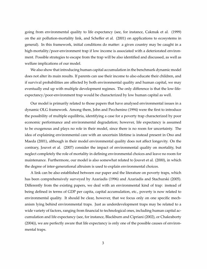
As reported in Figure 1, for our cross-section of 132 countries there is strong evidence sup-

porting the idea that longevity and environmental quality are linked; in particular, the correla-

tion coefficient is equal to 0.66 and statistically significant at the 1% level. The graph below is

compatible with the hypothesis of a two-way causality between the two variables.

30 40 50 60 70

4050

6070

80

correlation

Life Expectancy

EP

I (20

06)

ALB

DZA

AGO

ARG

ARM

AUSAUT

AZE

BGD

BEL

BEN

BOL

BRA

BGR

BFA

BDI

KHM

CMR

CAN

CAF

TCD

CHL

CHNCOL

COG

CRI

CIV

CUBCYP

CZE

COD

DNK

DOM

ECU

EGYSLV

ETH

FINFRA

GABGMB

GEO

DEU

GHA

GRC

GTM

GIN

GNB

HTI

HND

HUN

ISL

IND

IDN

IRN

IRL

ISR ITA

JAM

JPN

JOR

KAZ

KEN

KGZ

LAO

LBN

LBR

MDG

MWI

MYS

MLI

MRT

MEX

MDA

MNG

MAR

MOZ

MMR

NAM

NPL

NLDNZL

NIC

NERNGA

NOR

OMN

PAK

PAN

PNG

PRYPER PHL

POL

PRT

ROU

RUS

RWA

SAU

SEN

SLE

SVK

SVN

ZAF

KOR

ESP

LKA

SDN

SUR

SWZ

SWECHE

SYR

TJK

TZA

THA

TGO

TTO

TUN

TUR

TKM

UGA

UKR

ARE GBRUSA

UZB

VEN

VNM

YEM

ZMB ZWE

corr.coeff == 0.66

Figure 1: Environmental quality and life expectancySources: YCELP (2006), UN (2007)

In addition, a second kind of stylized fact is particularly interesting.

Stylized fact 2 Environmental quality and life expectancy are bimodally distributed across countries.

Therefore, the data suggest the possibility of an environmental poverty trap, characterized also

by short life expectancy. This concept points to the existence of "convergence clubs" in terms of

environmental performance and longevity: countries are concentrated around two levels of the

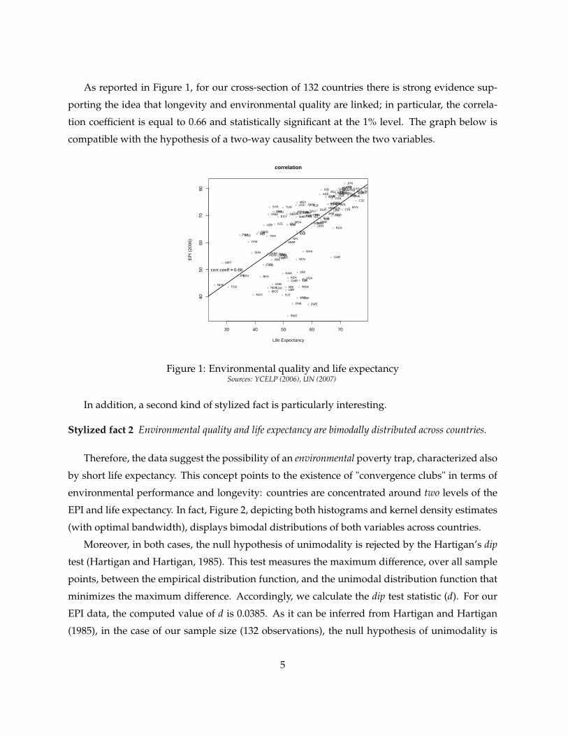
EPI and life expectancy. In fact, Figure 2, depicting both histograms and kernel density estimates

(with optimal bandwidth), displays bimodal distributions of both variables across countries.

Moreover, in both cases, the null hypothesis of unimodality is rejected by the Hartigan’s dip

test (Hartigan and Hartigan, 1985). This test measures the maximum difference, over all sample

points, between the empirical distribution function, and the unimodal distribution function that

minimizes the maximum difference. Accordingly, we calculate the dip test statistic (d). For our

EPI data, the computed value of d is 0.0385. As it can be inferred from Hartigan and Hartigan

(1985), in the case of our sample size (132 observations), the null hypothesis of unimodality is

5

bandwidth=3.9EPI (2006)

Den

sity

30 40 50 60 70 80

0.00

00.

005

0.01

00.

015

0.02

00.

025

0.03

00.

035

bandwidth=4.3Life expectancy (2005)

Den

sity

30 40 50 60 70 80

0.00

0.01

0.02

0.03

0.04

Figure 2: Bimodal distribution of environmental quality and life expectancySources: YCELP (2006), UN (2007)

rejected because d > 0.0370 (at the 5% significance level). Therefore, we can think the World

distribution of environmental quality to be bimodal. The same applies to life expectancy: on the

basis of our data, since d = 0.036, the Hartigan’s dip test allows us to reject the null hypothesis

of unimodality at the 10% significance level.

3 The benchmark model

We start by setting up a simple model where agents allocate their resources between current

consumption and environmental maintenance. Consumption, generating pollution and/or in-

creasing pressure on natural resources, determines some degradation of environmental quality.

No growth mechanism is considered.

3.1 Structure of the model

We consider an infinite-horizon economy that is populated by overlapping generations of agents

living for three periods: childhood, adulthood, and old age. Time is discrete and indexed by

t = 0, 1, 2, ..., ∞. All decisions are taken in the adult period of life. Individuals live safely through

the first two periods, while survival to the third period is subject to uncertainty. We assume no

population growth. Furthermore, agents are considered to be identical within each generation,

whose size is normalized to one (in the first two periods). Preferences are represented by the

6

following utility function, that we assume to be logarithmic to get closed-form solutions:

U(ct, et+1) = ln ct + πtγ ln et+1; (1)

people care about adult consumption (ct) and environmental quality when old (et+1); γ (> 0)

represents the weight agents give to the future environment (green preferences), while πt de-

notes the survival probability (that is taken as given since it depends on inherited environmental

quality). Here, for the sake of simplicity, we abstract from time discounting so that the subjective

preference for the future is entirely determined by πtγ. Notice also that in our framework an

increase (decrease) in the survival probability translates into a higher (lower) life expectancy, so

that hereafter we will use the two concepts interchangeably.

Let us underline that et may encompass both environmental conditions (quality of water, air

and soils, etc.) and resources availability (biodiversity, forestry, fisheries, etc.).3 Broadly speak-

ing, et can be seen as an index of the amenity (use and non-use) value of the environment. The

introduction of et+1 in the individual utility function is consistent with what Popp (2001) defines

as "weak altruism": agents decide to provide environmental quality for a combination of both

self-interest and the interest of future generations. In other words, people may be willing to en-

gage in environmental maintenance and improvement because they want themselves to enjoy a

better environment, and/or because they want to leave a better environment to their offspring.

Adult individuals face the following budget constraint:

wt = ct + mt; (2)

they allocate their income (wt) between consumption and environmental maintenance (mt). In

this benchmark version of our model, wt is assumed to be exogenous.4 Environmental mainte-

nance summarizes all the actions that agents can take in order to preserve and improve environ-

mental conditions.

Following John and Pecchenino (1994) and Ono (2002), the law of motion of environmental

quality is given by the following expression:

et+1 = (1− η)et +σmt −βct − λQt, (3)

with β,σ , λ > 0 and 0 < η < 1.3All these issues are taken into account by the EPI, that we have consistently used as a proxy of environmental

quality in Figures 1 and 2.4This assumption will be relaxed in Section 3, where we allow for human capital accumulation and consequent

income dynamics.

7

The parameter η is the natural rate of deterioration of the environment, σ represents the ef-

fectiveness of maintenance, whereas β accounts for the degradation of the environment, or pol-

lution, due to each unit of consumption. The above formulation also allows for the possibility of

external effects (coming from outside economies) on our environment: λQt > 0 (< 0) represents

the total impact of a harmful (beneficial) activity.5

Notice that a reduction in ct has a double effect on the environment: it directly affects envi-

ronmental quality through the parameterβ (alleviating the pressure on natural resources and/or

reducing pollution), and frees resources for maintenance (relaxing the budget constraint). More-

over, equation (3) implies that agents cannot, through their actions, modify the current state of

the environment (et). The latter is thus ”inherited”, depending only on the past generation’s

choices.6

3.2 Optimal choices

Taking as given wt, et and πt, agents choose ct and mt so as to maximize (1) subject to (2), (3),

ct > 0, mt > 0 and et > 0. Optimal choices are then given by:

mt =λQt − (1− η)et + [β+γ(β+σ)πt]wt

(β+σ)(1 +γπt), (4)

and

ct =(1− η)et +σwt − λQt

(β+σ)(1 +γπt). (5)

Notice that here, given that agents are identical and the population is normalized to one, ag-

gregate variables (choices) are completely equivalent to individual ones. Therefore, all variables

in our model can be also easily interpreted as "country" variables.

From (4) and (5), we can observe that both consumption and environmental maintenance are

positively affected by income: richer economies are more likely to invest in environmental care.

In addition, current environmental quality has a positive effect on consumption, but a negative

one on maintenance: investments in maintenance are less needed if the inherited environment is

less degraded. These two results have already been established by existing papers like John and

Pecchenino (1994) and Ono (2002).

5Episodes of acute pollution, like oil slicks or the Chernobyl disaster, can be typical examples of Qt > 0, whilethe implementation of an international agreement that promotes a worldwide reduction of pollutants (i.e. the KyotoProtocol) or the preservation of the Amazonian forest could be regarded as a negative Qt in our model.

6Therefore, our results would not change if we introduce current environmental quality (et) in the utility function.

8

The novelty of our model is that we can identify a specific effect of life expectancy (as deter-

mined by the survival probability πt) on environmental maintenance. As it can be easily seen

from the following derivative:

∂mt

∂πt=γ[(1− η)et +σwt − λQt]

(β+σ)(1 +γπt)2 , (6)

that is positive as soon as we have interior solutions, a higher survival probability raises stronger

concerns for the future state of the environment, thus inducing more maintenance.

In addition, a relatively larger value of Qt requires more investment in maintenance. Notice

that the term (1− η)et − λQt represents the net effect of past and external environmental condi-

tions on optimal choices.

3.3 Dynamics

Once we substitute (4) and (5) into (3), we get the following dynamic difference equation, de-

scribing the evolution of environmental quality over time:

et+1 =γπt

1 +γπt[(1− η)et +σwt − λQt]. (7)

Until now we have considered πt as exogenous, although we have pointed out that life ex-

pectancy may depend on (bequeathed) environmental quality. Now, we introduce explicitly a

function πt = π(et), such that π ′(·) > 0, lime→ 0 π(e) = π and lime→∞ π(e) = π ≤ 1. This for-

mulation is consistent with a large body of medical and epidemiological literature showing clear

effects of environmental conditions on adult mortality, like for instance Elo and Preston (1992),

Pope et al. (1995) and Evans and Smith (2005). The shape of π(et) may reflect "technological"

factors affecting the transformation of environmental quality into survival probability such as,

for instance, medicine effectiveness.

Notice that agents cannot improve their survival probability by investing in maintenance.

This is consistent with equation (3), where current environmental choices (especially mt) affect

the future state on the environment.7 Any investment in maintenance will be rewarded, in terms

of environmental quality and life expectancy, only in the future period. This introduces, in terms

of longevity, an inter-generational externality.

The dynamics of our model are now described by:

et+1 =γπ(et)

1 +γπ(et)[(1− η)et +σwt − λQt] ≡ φ(et). (8)

7Since mt determines et+1 (and not et), it looks sensible to have π(et), rather than π(mt), for instance.

9

In this framework, a steady-state equilibrium is defined as a fixed point e∗ such thatφ(e∗) =

e∗, which is stable (unstable) ifφ′(e∗) < 1 (> 1).

Depending on the shape of the transition function φ(et), we may have different scenarios.

For the sake of simplicity, we assume that wt and Qt are not only exogenous but also constant,

so that wt = w and Qt = Q. Figure 3 shows that we have only one stable steady-state as long

as φ(·) is concave for all possible values of et. Non-ergodicity and multiple steady-states may

instead occur ifφ(·) is first convex and then concave, displaying an inflection point. In this case,

depending on initial conditions, an economy may end up with either high or low environmental

quality (e∗H and e∗L, respectively).

0 et

et+1

e∗L e∗He

φ(Et)

Figure 3: Dynamics

Let us underline that a convex-concave transition function φ(et) might be generated by a

convex-concave survival probability π(et): under low environmental conditions, an improve-

ment of the environmental quality drives a small rise on the survival probability. However,

beyond an environmental threshold, this will translate into a much higher life expectancy. As-

suming such a functional form for π(et) is consistent with the idea that, for instance, the function

describing the effects of environmental degradation (be it increased pollution or exploitation of

resources) on a given ecosystem, or on human health, is itself convex-concave. Dasgupta and

Mäler (2003) explain that nature’s non-convexities are frequently the manifestation of feedback

effects, which might in turn imply the existence of ecological thresholds and therefore of mul-

tiple equilibria. Threshold-effects, sigmoid dose-response functions, non-smooth dynamics and

10

regime shifts in ecosystems are commonly assumed in natural sciences (see Scheffer et al. (2001),

for a comprehensive study).8 Finally, Baland and Platteau (1996) state that, in the case of natu-

ral resources involving ecological processes, there might well be threshold levels of exploitation

beyond which the whole system moves in a discontinuous way from one equilibrium to another.

3.4 Poverty trap: an analytical illustration

The possibility of multiple equilibria implies the existence of an environmental poverty trap. To

give an analytical illustration of such a case, we introduce now the following specific functional

form relating the survival probability to inherited environmental quality:

π(et) =

π if et < e

π if et ≥ e, (9)

where e is an exogenous threshold value of the environmental quality, above (below) which the

value of the survival probability is high (low). Obviously, we also assume that π > π . The

value of e may depend on factors such as medicine effectiveness, health care quality, etc. For

instance, a low e can be explained by a very efficient medical technology that makes long life

expectancy possible even under bad environmental conditions. On the contrary, a high e may

represent the case of a developing country where health services are so poorly performing that

any deterioration of the environment translates easily into higher mortality.

Given equation (9), the transition functionφ(et) becomes:

φ(et) =

γπ

1+γπ [(1− η)et +σw− λQ] if et < eγπ

1+γπ [(1− η)et +σw− λQ] if et ≥ e. (10)

We can then claim the following:

Proposition 1 If the following condition holds:

γπ

1 +γηπ<

eσw− λQ

<γπ

1 +γηπ,

then the dynamic equation (10) admits two stable steady-states e∗L and e∗H, such that e∗L < e < e∗H.

Proof. Provided that it exists, any steady-state is stable since, in our model, φ′(et) < 1, ∀et > 0.

Multiplicity arises if [γπ/(1 +γηπ)](σw− λQ) < e < [γπ/(1 +γηπ)](σw− λQ), which yields

the condition above.8The existence of a threshold effect in the relation between air-pollution and mortality has been also detected, for

instance, by Cakmak et al. (1999)

11

In particular, we will have that:

e∗L =γπ

(1 +γηπ)(σw− λQ) and e∗H =

γπ

(1 +γηπ)(σw− λQ). (11)

It can be easily seen that the steady-state value of environmental quality (be it low or high)

is positively affected by the survival probability (π or π) and by income w (via the parameter σ ,

representing the effectiveness of maintenance), while it is negatively influenced by the external

effect λQ.

The dynamics of our system is depicted in Figure 4. The threshold value e identifies a poverty

trap: an economy starting from an environmental quality between 0 and e will reach the equilib-

rium point A, which is a steady-state characterized by both low environmental quality (e∗L) and

short life expectancy (π). However, if initial conditions are such that e0 ≥ e, the economy will

end up in the "higher" steady-state B, where longer life expectancy (π) is associated with better

environmental quality (e∗H).

et+1

et0

A

B

B′

φ(et) = et

e∗L e∗He

Figure 4: Environmental poverty trap

The underlying mechanism goes as follows: for initial environmental quality below the thresh-

old value e, the survival probability is pinned down to π . As it has been previously discussed,

shorter life expectancy implies a weaker concern for the future: by optimal choices (4) and (5),

and for a given income, a lower survival probability induces agents to substitute environmental

12

maintenance with consumption. Therefore, from equation (10), environmental quality decreases,

ending up with the lower steady-state value e∗L. Symmetrically, if e0 ≥ e, our economy is driven

to e∗H.

3.5 In and out of the trap

It is interesting to analyse different possible strategies to escape from the environmental poverty

trap, as well as factors that could push some economies back to a low equilibrium characterized

by both a bad environment and low longevity.

Before doing so, let us just underline that the very existence of this kind of environmental

poverty trap implies that some countries (or regions) may even experience, over time, both en-

vironmental degradation and decay in life expectancy. Cross section data would suggest that

the latter is much less common than the former. The fact that, in some cases, environmental

degradation does not imply lower longevity, may be due to the fact that economic growth (ne-

glected until now in our analysis) might, at the same time, worsen environmental quality but

generate additional resources that can help increasing (or preserving) longevity. However, there

is also evidence of countries where environmental degradation is associated with a reduction in

life expectancy. For instance, McMichael et al. (2004) identify 40 countries that experienced a

loss in longevity between 1990 and 2001 (26 between 1980 and 2001);9 they also suggest that the

resulting World divergence in terms of life expectancy might be explained by " ... (the growing)

health risks consequent on large-scale environmental changes caused by human pressure". Not

surprisingly, most of those countries are African or ex-Soviet countries.

The fall in life expectancy (and increased mortality risk) in Africa has often been related to

mismanagement of environmental resources, pollution and anthropogenic climate change (see

Patz et al. (2005), among others). In the case of the ex-USSR, the argument for a pollution-

driven mortality resurgence has also been put forward, for instance, by Feachem (1994), and

Jedrychowski (1995).

Let us also mention the case - particularly cherished by economists - of Easter Island. This

small Pacific Island serves as a very good example of a closed system where insufficient envi-

ronmental care (or better, too much human pressure on the existing natural resources, especially

forestry) ultimately led to a dramatic reduction of the local population (see Diamond (2005) for

a general presentation, or de la Croix and Dottori (2008)).

9Losses in life expectancy are sometimes severe, going up to 15-18 years.

13

3.5.1 Escaping the trap

Let us assume that our economy is initially trapped in the "low" steady-state A, characterized

by bad environmental quality and short life expectancy (e∗L, π). Technically speaking, we can

identify different ways of escaping this trap.

First, as it is clear from Figure 4, a large enough permanent reduction in the environmental

threshold value e, such that e becomes lower than e∗L, will eliminate the low steady-state, thus

driving our economy toward the high steady-state B. As we observed in Section 2.1, this may

correspond, for instance, to an improvement in medicine effectiveness.10 The crucial point is that

in this new situation, the survival probability associated to e∗L is π instead of π . This implies

greater concern about the future, more maintenance (equation (6)), less consumption, and finally

convergence to the high (and now unique) steady-state B identified by (e∗H , π).

Second, for a fixed e, our economy can still get away from the poverty trap by means of a

parallel shift-up of the transition functionφ(et) such that the low steady-state A disappears (see

Figure 4). As it can be inferred from equation (10), such an upwards shift ofφ(et) may be induced

by (i) a permanent income expansion, and/or (ii) a permanent reduction of harmful external effects

on the environment.11 A possible real world example of a smaller Q could be the global reduction

in pollution due to the implementation of international environmental agreements, such as the

Kyoto Protocol.

Third, the inferior steady-state A can be also eliminated if the slope of φ(et) increases for

et ∈ (0, e). A steeper transition function may be explained, for instance, by a permanent rise in

the survival probability in a deteriorated environment (π) that, similarly to the reduction of e

mentioned above, can be traced back to technological progress in medical sciences, etc.

3.5.2 Back in the trap?

Intuitively, all the mechanisms we have seen above may work in the opposite direction. For

instance, a reduction in w and/or an increase in Q may lead to the elimination of the high steady-

state (B in Figure 4) and the economy, that would have otherwise converged to the higher steady-

state, can be thrown back in the poverty trap.

10De la Croix and Sommacal (2008) have a model in which a rise in medicine effectiveness, through a longer life ex-pectancy, promotes capital accumulation and income growth. In our setting, advances in medicine induce a differentkind of investment, i.e. environmental maintenance and improvement.

11Even a temporary reduction in Q can help leaving the trap. In this case, however, escaping from the trap does notimply the elimination of the lower steady-state.

14

It is worth noticing that even temporary variations of initial conditions may be sufficient to

fall into the trap. Referring to Figure 4, suppose that the environmental quality of our economy

belongs to a small right neighbourhood of e: out of external intervention, the economy would

converge to the high steady-state B. However, any event susceptible of reducing e0 below e

pushes the economy into "vicious" dynamics, involving a deterioration of both environmental

conditions and life expectancy. Examples of such events may range from natural disasters to

episodes of very acute pollution.

This should raise a concern about the environmental awareness of countries. Neglecting envi-

ronmental care, bad management of natural resources and too much exposure to environmental

risks, may make countries vulnerable to even temporary events with serious long-lasting con-

sequences: in particular, countries with a somewhat fragile environment are prone to pay high

costs in terms of human development through lower life expectancy.

Furthermore, some countries might happen to be caught in the trap if they meet environmen-

tal constraints when life expectancy is still low. This could be the case of those African countries

which display a low life expectancy, but are already very polluted.

3.6 Welfare analysis

In our model, agents are outlived by the consequences of their environmental choices, and they

are not able to internalize the external effects of these choices on future generations. It would then

be interesting to compare such a decentralized equilibrium with a "green" golden rule allocation,

as defined by Chichilnisky et al. (1995). This means solving the model from the point of view of

a myopic social planner, whose objective is to maximize aggregate utility in each period, thereby

treating all generations symmetrically.12

The green golden rule allocation can be found by solving the problem of such a social planner

at the steady-state, as in John and Pecchenino (1994). We then look for the optimal steady-state

combination of consumption and environmental quality that maximizes:

U(c, e) = ln c + π(e)γ ln e, (12)

subject to:

w = c + m, (13)

12A fullfledged forward looking planner would develop an optimal intertemporal plan, but this is not central toour analysis.

15

and

ηe = σm−βc− λQ, (14)

where π(e) can be either π or π , while (13) and (14) represent, respectively, the budget and the

environmental constraints at the steady-state.

Eliminating m and solving for c we obtain:

c =−ηe +σw− λQ

β+σ, (15)

which gives consumption as a function of e, in any steady-state.

After replacing c in the utility function and solving the first-order condition ∂U/∂e = 0, we

can determine the following "golden" value for environmental quality (in our case, the condition

∂2U/∂e2 < 0 always holds):

eg =γπ

(1 +γπ)η(σw− λQ). (16)

Let us now compare this golden allocation with the decentralized solution and describe the

dynamics of the model in the two cases. In Figure 5, we represent as a solid line the transition

function in the decentralized economy, while the dotted line represents the dynamic evolution

of e under the social planner hypothesis. Notice that the planner maximizes utility at the begin-

ning of each period, and therefore takes π as given, since the latter is fully determined by past

environmental quality.13

Suppose that the decentralized economy produces multiple equilibria. Depending on the

value of e, we may have two different scenarios. If e is sufficiently larger than e∗L (the level of

environmental quality that characterizes the low decentralized steady-state), as in Figure 5a, then

there will also be two golden rule allocations, each one superior to the corresponding competitive

equilibrium. In fact, since η < 1, e∗L (e∗H) is lower than egL (eg

H), obtained replacing π with π (π) in

(16). If instead e is quite close to e∗L (e′ in Figure 5b), then it can happen that there exists a unique

green golden rule allocation: in this case, we may say that the social planner is able to eliminate

the lower steady-state, thus driving the economy out of the trap.

We can then claim the following:

Proposition 2 At the steady-state, a decentralized equilibrium involves lower environmental qualitythan the "green" golden rule allocation. Moreover, under proper conditions, the social planner solutionmay imply the elimination of the environmental trap.

13This is the main difference with a non-myopic planner, who is able to formulate an optimal intertemporal plan.

16

et+1

et0

φ(et) = et

egL e∗He egHe∗L

(a)

et+1

et0

φ(et) = et

e∗L e∗He′ egH

(b)

Figure 5: The "green" golden rule

The decentralized economy is under-investing in maintenance since agents do not internalize

the positive effect of environmental care on the welfare of forthcoming generations. Not surpris-

ingly, the "distance" between the decentralized and the golden rule values of e is inversely related

to η. At the limit, as η tends to 1, the effect of past environmental quality on the current state

of the environment tends to disappear (thus, eliminating the inter-generational externality), and

therefore the decentralized solution approaches the golden-rule allocation.

4 Introducing human capital accumulation

In the basic version of our model, income was completely exogenous in every period and we did

not allow for any growth mechanism. In this Section, we aim at overcoming these two limitations

by introducing human capital accumulation through education. We want to capture three rather

simple ideas: (i) environmental preservation subtracts some resources not only from consump-

tion but also from investment, (ii) income growth, relaxing the budget constraint, makes more

maintenance possible, and (iii) growth might itself involve some pollution.14

14We could tell the same story if we had physical capital instead of human capital.

17

4.1 Structure of the model

Agents maximize the following utility function:

U = ln ct + πt(α ln ht+1 +γ ln et+1). (17)

With respect to (1), we have introduced explicitly inter-generational altruism: parents care

about the human capital level attained by their children (ht+1); the importance attached to this

term is measured by α, with 0 < α < 1. Inter-generational altruism is eventually magnified

(reduced) by a higher (lower) πt: the success (or failure) of their children will affect relatively

more those parents who will live long enough to witness it. Once more, for the sake of simplicity,

we neglect inter-temporal discounting, so that the preference for the future is completely defined

by the survival probability.

An increased survival probability implies that agents value more future environmental qual-

ity, exactly as it was in the basic model. Moreover, it now makes agents more sympathetic to

their offspring, reinforcing inter-generational altruism.

Production of a homogeneous good takes place according to the following function:

yt = wht, (18)

where w, that we assume to stay constant over time, is both an index of productivity and the

wage rate; ht is also aggregate human capital, once we normalize to 1 the population of our

economy. As before, fertility is exogenous, constant and such that there is no population growth.

The budget constraint writes as:

wht = ct + mt + vt. (19)

Agents are paid w for each unit of human capital. Available income may be employed for three

alternative purposes: current consumption (ct), environmental maintenance (mt) and educational

investment (vt). More precisely, vt denotes the total amount of education bought by parents for

their children, assuming that education is privately funded.

Education is pursued by parents because it can be transformed into future human capital

according to the following function:

ht+1 = δhθt (µ + vt)1−θ , (20)

where, depending on θ (with 0 < θ < 1), ”nature” (parental human capital ht) complements

”nurture” (vt) in the accumulation of productive skills. Notice that δ (> 0) accounts for total

18

factor productivity in human capital accumulation, while the parameter µ (> 0) prevents human

capital from being zero even if parents do not invest in education, as in de la Croix and Doepke

(2003, 2004).

Agents engage in environmental maintenance because it helps to improve future environ-

mental quality, according to:

et+1 = (1− η)et +σmt −βct −ψyt. (21)

This formulation reproduces (3), with two exceptions: we have now added a factor accounting

for growth-induced pollution (through the coefficient ψ > 0), while the term representing ex-

ternal effects has been removed for ease of presentation. Notice that here, differently from the

benchmark version of our model, we have introduced explicitly a production function. It then

would seem perfectly reasonable to consider that such production can also, to some extent, affect

environmental quality. Therefore, we have now two potential sources of pollution: consumption

and production. As in the real world, both consumers and firms are susceptible to degrading

the environment through their actions. We assume for the moment ψ < σ , thus implying that

the environmental benefit produced by one unit of maintenance is larger than the environmental

damage caused by one unit of production. This looks reasonable, since maintenance is com-

pletely dedicated to improving the environment, while production generates pollution only as a

"by-product".

4.2 Optimal choices

Maximizing (17) subject to (19), (20), (21), ct > 0, mt > 0, et > 0 and ht > 0, leads to the following

optimal choices:

mt =σ [β+γ(β+σ)πt](µ + wht) + [σ + (β+σ)α(1−θ)]ψwht − (1− η)[σ +α(1−θ)(β+σ)πt]et

σ(β+σ){1 + [α(1−θ) + γ]πt},

(22)

vt ={α(1−θ)[(1− η)et + (σ −ψ)wht]−γµσ}πt −µσ

σ{1 + [α(1−θ) +γ]πt}, (23)

and

ct =(1− η)et +µσ + (σ −ψ)wht

(β+σ){1 + [α(1−θ) + γ]πt}. (24)

First of all, it is interesting to compare (22) with (4): the negative association between main-

tenance and current environmental quality still holds, as well as the positive effect of income,

which is now related to current human capital. All other things being equal, human capital ac-

cumulation makes more resources available for environmental care. Of course, investment in

19

maintenance is negatively affected by α, reflecting the relative substitutability between future

human capital and future environmental quality in the utility function. Finally, the positive effect

of life expectancy on environmental maintenance is confirmed, provided that:

γσ > α(1−θ)β, (25)

as it can be inferred from:

∂mt

∂πt=

[γσ −α(1−θ)β][(1− η)et +µσ + (σ −ψ)wht)]σ(β+σ){1 + [α(1−θ) + γ]πt}2 . (26)

Condition (25), which we assume to hold henceforth, requires that the preference for environ-

mental quality and the effectiveness of maintenance (γ and σ , respectively) must be strong

enough to compensate for the weight attached to education (both in the utility function, through

α, and in human capital formation, through (1−θ)) and the detrimental effect of consumption

on the environment (β).

Parental investment in education depends positively on both human capital (because of the

traditional income effect and the inter-generational externality in education) and current envi-

ronmental quality. If the latter is good enough, requiring a smaller investment in maintenance, it

frees resources that can be allocated to education. Moreover, as expected, longer life expectancy

induces stronger investment in human capital.15 In fact, the following derivative is always posi-

tive (under the assumption that ψ < σ):

∂vt

∂πt=α(1−θ)[(1− η)et +µσ + (σ −ψ)wht)]

σ{1 + [α(1−θ) + γ]πt}2 . (27)

4.3 Dynamics

By replacing (22)-(24) into (20) and (21) we get the following non-linear system of two difference

equations which describes the dynamics of our economy:

ht+1 = δhθt

(α(1−θ)[(1− η)et +µσ + (σ −ψ)wht)]πt

σ{1 + [α(1−θ) + γ]πt}

)1−θ≡ ξ(ht, et), (28)

15This result, that we obtain for parentally-funded education, is quite common in the literature, although it may bemotivated by somewhat different reasons. For instance, Galor (2005, p. 231) claims that "... the rise in the expectedlength of the productive life may have increased the potential rate of return to investments in children’s humancapital, and thus could have induced an increase in human capital formation ...". The positive effect of life expectancyon human capital accumulation can be also generalized to self-funded education: since Ben Porath (1967), it has beenwell established that the expectation of a longer productive life induces agents to invest more in their own humancapital.

20

et+1 =γ[(1− η)et +µσ + (σ −ψ)wht)]πt

1 + [α(1−θ) + γ]πt≡ ψ(ht, et). (29)

In this set-up, a steady-state equilibrium is defined as a fixed point (h∗, e∗) such thatξ(h∗, e∗) =

h∗ and ψ(h∗, e∗) = e∗. Similarly to Section 3, we assume the following functional form for the

survival probability:

πt(ht, et) =

π if et +κht < J

π if et +κht ≥ J, (30)

with κ, J > 0.

This formulation captures the substitutability (accounted for by κ) between human capital

and environmental quality in increasing life expectancy. Notice also that J is an exogenous

threshold value. In Section 3, we have explained how environmental conditions could improve

survival probabilities. However, now we also assume that each agent’s probability of survival is

positively related to his own human capital. Such a mechanism has already been exploited by,

for instance, Blackburn and Cipriani (2002) and de la Croix and Licandro (2007), in theoretical

models linking growth and demographic dynamics. Apart from the obvious income effect, the

positive influence of human capital on longevity may be justified by the fact that better educated

people have access to better information about health, are less likely to take up unhealthy be-

haviour, such as smoking, becoming overweight, etc. It is also consistent with the findings of

several empirical studies like, for instance, Lleras-Muney (2005).

Equation (30) paves the way to the existence of multiple steady-states, i.e. multiple solutions

to the system composed by equations (28) and (29). After defining the two loci HH ≡ {(ht, et) :

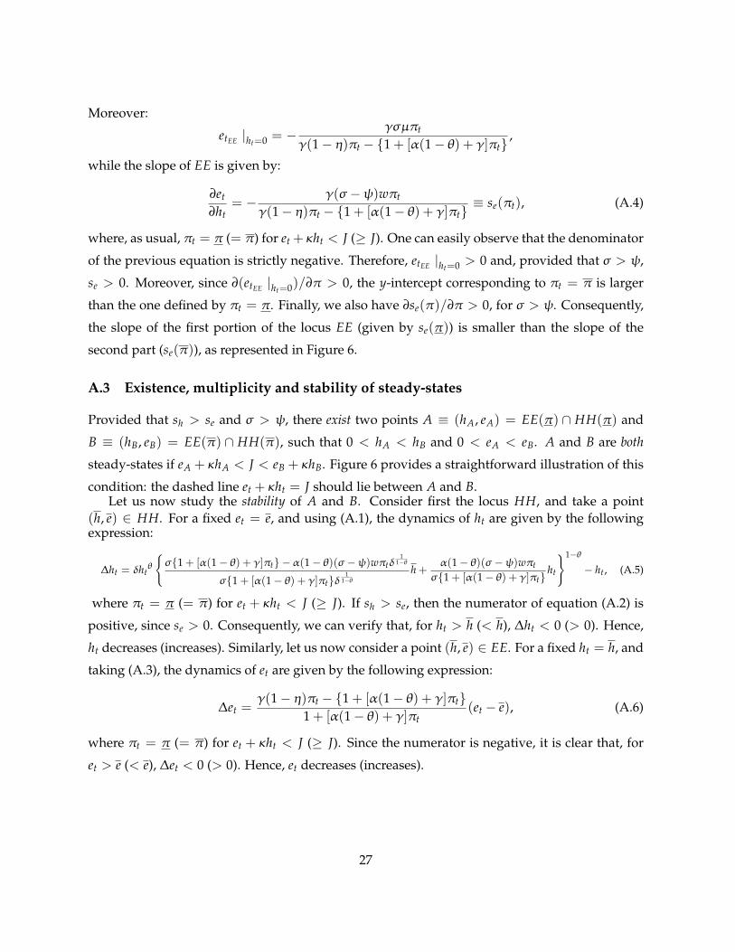
ht+1 = ht} and EE ≡ {(ht, et) : et+1 = et}, we can claim the following:

Proposition 3 Provided that (i) σ > ψ, (ii) proper conditions on the threshold value J hold, and (iii) theslope of HH is larger than the slope of EE, then there exist two stable steady-states A and B such that0 < h∗A < h∗B and 0 < e∗A < e∗B.

Proof. See Appendix A

In particular, the "high" equilibrium is characterized by:

e∗B =γµσ2π

σ + {γησ + [σ − δ 11−θ (σ −ψ)w]α(1−θ)}π

, (31)

and

h∗B =α(1−θ)δ 1

1−θµσ2π

σ + {γησ + [σ − δ 11−θ (σ −ψ)w]α(1−θ)}π

; (32)

21

while to obtain the "low" equilibrium (h∗A, e∗A) we just need to replace in the above expressions π

with π . Notice that wδ1/(1−θ) < σ/(σ −ψ) is a sufficient condition for both steady-state values

to be strictly positive. Moreover, it also ensures that the slope of HH is positive (see Appendix

A).

It can be shown that the steady-state values of both environmental quality and human capital

are positively affected by π and w, provided that ψ < σ . Concerning the other parameters, it

is interesting to underline that e∗ depends positively on θ: the more important is nature (with

respect to nurture) in human capital formation, the more parents will be likely to invest in main-

tenance (rather than in education). Obviously, α and γ also influence positively the long-run

levels of human capital and environmental care, respectively.

Let us now give a quick description of the behaviour of our dynamical system. An economy

starting from an environmental quality (e0) and parental human capital (h0) low (high) enough

(e0 +κh0 < (≥)J) will end-up in the steady-state equilibrium A (B), which is characterized by

both low (high) environmental quality and human capital, and short (longer) life expectancy.

Such a situation is represented by the phase diagram in Figure 6.

et

ht0

J

A

B

HH

EE

Figure 6: Phase diagram

The causal relationship linking the survival probability to both environmental quality and

22

human capital implies the possibility of a country being trapped in an environmental poverty

trap, as in the benchmark model, and the underlying mechanism is quite similar. However, the

poverty trap is now characterized by three elements, namely, low levels of: (i) environmental

quality, (ii) life expectancy, and (iii) human capital.16

By consequence, differently from Section 3, an economy initially trapped in the "inferior"

steady-state can get out of it also through exogenous factors or policies that are related to human

capital. We may think of, amongst others, the introduction of public schooling or educational

subsidies, or of an exogenous increase in the productivity of the schooling system (δ). In Figure

6 the latter would correspond, for instance, to a repositioning of the EE and HH loci, such that

(h0, e0) may fall in the basin of attraction of B instead of A.

Nevertheless, as in Section 3, an economy out of the poverty trap is not safe forever and

human capital can be interpreted as an additional "risk factor": a given country may fall into the

environmental trap as a consequence, for instance, of a massive destruction of human capital.

4.4 Welfare analysis

Here we want to find the "green" golden-rule allocation and compare it with the equilibrium of

the decentralized economy, where agents did not internalize the effects of their actions on the

welfare of following generations. We will proceed as we did in Section 3.6, by solving, at the

steady-state, the problem of a myopic social planner who treats all generations symmetrically,

striving to maximize aggregate utility in every period.

Therefore, we look for the optimal steady-state combination of consumption, environmental

quality and human capital that maximizes:

U(c, e, h) = ln c + π(e)(α ln h +γ ln e), (33)

subject to:

wh = c + m + v, (34)

ηe = σm−βc−ψwh, (35)

and

h = δhθ(v +µ)1−θ , (36)

16This result is consistent with stylized facts, which suggest a bimodal distribution of human capital as well. Dataare available upon request.

23

where (34) and (35) are, respectively, the budget and the environmental constraints at the steady-

state, while (36) is the stationary production function for human capital. Notice also that π(e)

can be either π or π .

Eliminating m and v, and solving for c, we obtain:

c =−ηe +µσ + [(σ −ψ)w−σδ 1

θ−1 ]hβ+σ

. (37)

After replacing c in the utility function, we can solve the system made of the two first-order

conditions ∂U/∂e = 0 and ∂U/∂h = 0 to obtain:

eg =αµσπ

η[1 + (α +γ)π ](38)

and

hg =αµσπ

[σδ1θ−1 − (σ −ψ)w][1 + (α +γ)π ]

. (39)

We are ensured that this solution represents a maximum since: ∂2U/∂e2 < 0 and ∂2U/∂h2 <

0. After comparing eg with e∗, we can claim the following:

Proposition 4 At the steady-state, for sufficiently low values of η, the decentralized equilibrium involveslower environmental quality than the "green" golden rule allocation. Moreover, under proper conditions,the social planner solution may imply the elimination of the environmental trap.

In particular, we need η < η, where:

η ≡ σ + [σ − δ 11−θ (σ −ψ)w]α(1−θ)πσ(1 +απ)

. (40)

Provided that the stability condition mentioned in Proposition 3 holds, η is positive. Moreover,

for α tending to 0, η tends to 1, thus reproducing the case analysed in Section 3.6. This is not

surprising, sinceα represents the weight of human capital in the utility function.

Moreover, depending on how much the decentralized low steady-state is close to J (other-

wise said, J − (e∗A + κh∗A) should be sufficiently small), there is the possibility that the golden

rule allocation is unique. In other words, a social planner who internalizes inter-generational

externalities might be able to drive the economy out of the trap.

The dynamic mechanism producing this result can be seen as a straightforward two-dimensional

translation of the one that has been analysed in Section 3.6.

24

5 Conclusions

In this paper we have studied the interplay between life expectancy and the environment, as well

as its dynamic implications. The basic mechanism, upon which our theoretical model is built, is

very simple. On the one hand, environmental quality depends on life expectancy, since agents

who expect to live longer have a stronger concern for the future and therefore invest more in

environmental care. On the other hand, it is reasonable to presume that longevity is affected by

environmental conditions. By modelling environmental quality as an asset that can be accumu-

lated over time, we have shown that life expectancy and environmental dynamics can be jointly

determined, and multiple equilibria may arise. In particular, we have focused on the existence

of an environmental kind of poverty trap, characterized by both low life expectancy and poor

environmental performance. Possible "escape" strategies, as well as factors affecting the risk to

be caught in such a trap, have been discussed. Both the correlation between environmental per-

formance and life expectancy, and possible non-ergodic dynamics, are consistent with stylized

facts.

Our model is also robust to the introduction of a very simple growth mechanism via human

capital accumulation. If education depends on life expectancy, and survival probabilities are

affected by both environmental quality and human capital, we can always end up with multiple

development regimes, the only difference being that the low-life-expectancy/poor-environment

trap would be characterized by low human capital as well.

Moreover, some welfare analysis of the model suggests that the decentralized equilbrium is

inefficient: agents do not internalize the effects of their choices on future generations. Therefore, a

social planner who internalizes inter-generational externalities might achieve a superior equilib-

rium and, under proper conditions, might be able to drive the economy out of an environmental

poverty trap.

Finally, as interesting extensions and possible directions for further research, we would sug-

gest: (i) to introduce heterogeneity among agents, moving from a representative agent set-up to

a political economy model, where environmental choices are determined through voting; (ii) to

enhance the demographic part of the model, allowing for endogenous fertility and relating envi-

ronmental quality to demographic factors other than longevity (population density, for instance).

25

Appendices

A Proof of Proposition 3

The proof is organized as follows. We will first characterize the two loci HH and EE, and then

analyse the existence, multiplicity and stability of the steady-state equilibria.

Let us recall the definition of the two loci: HH ≡ {(ht, et) : ht+1 = ht} and EE ≡ {(ht, et) :

et+1 = et}.

A.1 Locus HH

From equation (28) we get that ht+1 − ht = ξ(ht, et) − ht, where πt is given by equation (30).

Therefore, the locus HH writes as:

et = − σµ

1− η +σ{1 + [α(1−θ) +γ]πt} −α(1−θ)(σ −ψ)wπtδ

11−θ

α(1−θ)(1− η)πtδ1

1−θht, (A.1)

where πt = π (= π) for et +κht < J (≥ J). As we can see in Figure 6, locus HH is a discontinuous

function divided into two parts (both straight lines) by et = J −κht. Its intersection with the y-

axis (i.e. the intercept) is given by etHH |ht=0 = −σµ/(1−µ) < 0, while its slope can be expressed

as:∂et

∂ht=σ{1 + [α(1−θ) + γ]πt} −α(1−θ)(σ −ψ)wπtδ

11−θ

α(1−θ)(1− η)πtδ1

1−θ≡ sh(πt), (A.2)

where πt = π (= π) for et + κht < J (≥ J). Indeed, as it is clear from the above equation, for

sh to be positive, we just need to have a positive numerator. Moreover, one can also verify that

∂sh(π)/∂π < 0. This implies that the first portion of the locus HH (given by sh(π)) is steeper

than the second one (sh(π)), as depicted in Figure 6.

A.2 Locus EE

Equation (29) yields et+1 − et = ψ(ht, et)− et, where πt is given by equation (30). Therefore, the

locus EE can be written as:

et = − γσµπt

γ(1− η)πt − {1 + [α(1−θ) + γ]πt}− γ(σ −ψ)wπt

γ(1− η)πt − {1 + [α(1−θ) +γ]πt}ht, (A.3)

where πt = π (= π) for et + κht < J (≥ J). As it happened for HH, the locus EE is also a

discontinuous function divided into two different parts (once more straight lines) by et = J−κht.

26

Moreover:

etEE |ht=0 = − γσµπt

γ(1− η)πt − {1 + [α(1−θ) + γ]πt},

while the slope of EE is given by:

∂et

∂ht= − γ(σ −ψ)wπt

γ(1− η)πt − {1 + [α(1−θ) + γ]πt}≡ se(πt), (A.4)

where, as usual, πt = π (= π) for et +κht < J (≥ J). One can easily observe that the denominator

of the previous equation is strictly negative. Therefore, etEE |ht=0 > 0 and, provided that σ > ψ,

se > 0. Moreover, since ∂(etEE |ht=0)/∂π > 0, the y-intercept corresponding to πt = π is larger

than the one defined by πt = π . Finally, we also have ∂se(π)/∂π > 0, for σ > ψ. Consequently,

the slope of the first portion of the locus EE (given by se(π)) is smaller than the slope of the

second part (se(π)), as represented in Figure 6.

A.3 Existence, multiplicity and stability of steady-states

Provided that sh > se and σ > ψ, there exist two points A ≡ (hA, eA) = EE(π) ∩ HH(π) and

B ≡ (hB, eB) = EE(π) ∩ HH(π), such that 0 < hA < hB and 0 < eA < eB. A and B are both

steady-states if eA +κhA < J < eB +κhB. Figure 6 provides a straightforward illustration of this

condition: the dashed line et +κht = J should lie between A and B.Let us now study the stability of A and B. Consider first the locus HH, and take a point

(h, e) ∈ HH. For a fixed et = e, and using (A.1), the dynamics of ht are given by the followingexpression:

∆ht = δhtθ

{σ{1 + [α(1−θ) +γ]πt} −α(1−θ)(σ −ψ)wπtδ

11−θ

σ{1 + [α(1−θ) + γ]πt}δ1

1−θh +

α(1−θ)(σ −ψ)wπtσ{1 + [α(1−θ) +γ]πt}

ht

}1−θ

− ht , (A.5)

where πt = π (= π) for et +κht < J (≥ J). If sh > se, then the numerator of equation (A.2) is

positive, since se > 0. Consequently, we can verify that, for ht > h (< h), ∆ht < 0 (> 0). Hence,

ht decreases (increases). Similarly, let us now consider a point (h, e) ∈ EE. For a fixed ht = h, and

taking (A.3), the dynamics of et are given by the following expression:

∆et =γ(1− η)πt − {1 + [α(1−θ) +γ]πt}

1 + [α(1−θ) + γ]πt(et − e), (A.6)

where πt = π (= π) for et +κht < J (≥ J). Since the numerator is negative, it is clear that, for

et > e (< e), ∆et < 0 (> 0). Hence, et decreases (increases).

27

References

[1] Azariadis, C. (1996): ”The economics of poverty traps. Part one: complete markets”, Journal

of Economic Growth 1, 449-486.

[2] Azariadis, C. and J. Stachurski (2005): ”Poverty traps”, in Aghion, P. and S.N. Durlauf (eds.):

Handbook of Economic Growth 1 (1), 295-384.

[3] Baland, J.-M. and J.-P. Platteau (1996): Halting the degradation of natural resources: is there a role

for rural communities, Clarendon Press, Oxford, UK.

[4] Ben Porath, Y. (1967): ”The production of human capital and the life cycle of earnings”,

Journal of Political Economy 75, 352-365.

[5] Blackburn, K. and G.P. Cipriani (2002): ”A model of longevity, fertility and growth”, Journal

of Economic Dynamics & Control 26, 187-204.

[6] Cakmak,S., R.T. Burnett and D. Krewski (1999): ”Methods for detecting and estimating pop-

ulation threshold concentrations for air pollution-related mortality with exposure measure-

ment error”, Risk Analysis 19 (3), 487-496.

[7] Chakraborty, S. (2004): ”Endogenous lifetime and economic growth”, Journal of Economic

Theory 116, 119-137.

[8] Chichilnisky, G., G. Heal and A. Beltratti (1995): ”The green golden rule”, Economics Letters

49, 175-179.

[9] Dasgupta, P. and K.-G. Mäler (2003): ”The economics of non-convex ecosystems: Introduc-

tion”, Environmental and Resource Economics 26, 499-525.

[10] de la Croix, D. and M. Doepke (2003): ”Inequality and growth: why differential fertility

matters”, American Economic Review 93 (4), 1091-1113.

[11] de la Croix, D. and M. Doepke (2004): ”Public versus private education when differential

fertility matters”, Journal of Development Economics 73, 607-629.

[12] de la Croix, D. and D. Dottori (2008): ”Easter Island collapse: a tale of population race”,

Journal of Economic Growth 13, 27-55.

28

[13] de la Croix, D. and O. Licandro (2007): ”’The child is father of the man’: implications for the

demographic transition”, mimeo.

[14] de la Croix, D. and A. Sommacal (2008): ”A theory of medical effectiveness, differential

mortality, income inequality and growth for the pre-industrial England”, Mathematical Pop-

ulation Studies forthcoming.

[15] Diamond, J. (2005): Collapse: how societies choose to fail or survive, Viking Books, New York,

NY.

[16] Elo, I.T. and S.H. Preston (1992): ”Effects of early-life conditions on adult mortality: a re-

view”, Population Index 58 (2), 186-212.

[17] Evans, M.F. and V.K. Smith (2005): ”Do new health conditions support mortality-air pollu-

tion effects?”, Journal of Environmental Economics and Management 50, 496-518.

[18] Feachem, R. (1994): ”Health decline in Eastern Europe”, Nature 367, 313-314.

[19] Galor, O. (2005): ”From stagnation to growth: unified growth theory”, in Aghion, P. and

S.N. Durlauf (eds.): Handbook of Economic Growth 1 (1), 171-293.

[20] Hartigan, J.A. and P.M. Hartigan (1985): ”The dip test of unimodality”, Annals of Statistics

13, 70-84.

[21] Jedrychowski, W. (1995): ”Review of recent studies from Central and Eastern Europe associ-

ating respiratory health effects with high levels of exposure to "traditional" air pollutants”,

Environmental Health Perspectives 103 (suppl. 2), 15-21.

[22] Jouvet, P.-A., Ph. Michel and J.-P. Vidal (2000): ”Intergenerational altruism and the environ-

ment”, Scandinavian Journal of Economics 102 (1), 135-150.

[23] Jouvet, P.-A., P. Pestieau and G. Ponthière (2007): ”Longevity and environmental quality in

an OLG model”, CORE Discussion Paper 2007/69.

[24] Lleras-Muney, A. (2005): ”The relationship between education and adult mortality in the

United States”, Review of Economic Studies 72, 189-221.

[25] McMichael, A.J., M. McKee, V. Shkolnikov and T. Valkonen (2004): ”Mortality trends and

setbacks: global convergence or divergence?”, Lancet 363, 1155-1159.

29

[26] Ono, T. (2002): ”The effects of emission permits on growth and the environment?”, Environ-

mental and Resource Economics 21, 75-87.

[27] Ono, T. and Y. Maeda (2001): ”Is aging harmful to the environment?”, Environmental and

Resource Economics 20, 113-127.

[28] Patz, J.A., D. Campbell-Lendrum, T. Holloway and J.A. Foley (2005): ”Impact of regional

climate change on human health”, Nature 438, 310-317.

[29] Pecchenino, R. and A. John (1994): ”An overlapping generations model of growth and the

environment”, Economic Journal 104, 1393-1410.

[30] Pope, C.A. III, D.V. Bates and M.E. Raizenne (1995): ”Health effects of particulate air pollu-

tion: time for reassessment?”, Environmental Health Perspectives 103 (5), 472-480.

[31] Popp, D. (2001): ”Altruism and the demand for environmental quality”, Land Economics 77

(3), 339-349.

[32] Scheffer, M., S. Carpenter, J.A. Foley, C. Folke and B. Walker (2001): ”Catastrophic shifts in

ecosystems”, Nature 413, 591-596.

[33] United Nations (2007): World Population Prospects: the 2006 revision. [Data available on-line

at http://unstats.un.org/unsd/demographic/products/socind/health.htm]

[34] Yale Center for Environmental Law and Policy (2006): Environmental Performance Index.

[Data available on-line at http://epi.yale.edu]

30