Lighthill-Whitham-Richards tra c ow model · Highway Capacity Manual Triangular: q = minfu f k;w(k j k)g Trapezoidal: q = minfu f k;q ... LWR Model Newell-Daganzo Method. With a more

Lighthill-Whitham-Richards traffic flow model

CE 392D

LWR Model

OUTLINE

1 Hydrodynamic model (LWR)

2 Shockwaves

3 Characteristics

4 Newell-Daganzo method

LWR Model Outline

The Lighthill-Whitham-Richards model is commonly usedfor traffic flow.

There are three fundamental variables:

Flow q, the rate at which vehicles pass a point.

Density k , the spatial concentration of vehicles.

Speed u, the average rate of travel.

It is also useful to track N, the vehicle number or cumulative count at apoint.

LWR Model Outline

These quantities can be visualized on a trajectory diagram.

The trajectories represent contours of N.

LWR Model Outline

The flow q is the rate trajectories cross a horizontal line.

LWR Model Outline

The density k is the rate trajectories cross a vertical line.

How is speed represented in a trajectory diagram?

LWR Model Outline

In a link model, we are often given initial conditions (density values att = 0) and boundary conditions (flow rates at x = 0, restrictions on flowrates at the downstream end.)

The task is to determine the outflows at the downstream end of the link;this may include finding N, q, k , and u at all points x and times t. Wecan treat these variables as functions of x and t.

LWR Model Outline

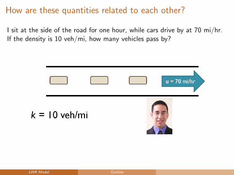
How are these quantities related to each other?

I sit at the side of the road for one hour, while cars drive by at 70 mi/hr.If the density is 10 veh/mi, how many vehicles pass by?

LWR Model Outline

This is a demonstration of the fundamental relationship between speed,flow, and density:

q = uk

Think units: [veh/hr] = [mi/hr][veh/mi]

LWR Model Outline

Flow and density are related to the cumulative counts:

q(x , t) =∂N(x , t)

∂t

k(x , t) = −∂N(x , t)

∂x

LWR Model Outline

If N is twice continuously differentiable,

∂2N

∂x∂t=

∂2N

∂t∂x

Therefore∂q

∂x+

∂k

∂t= 0

This is one way to derive the conservation equation. This equation holdseverywhere these derivatives exist.

LWR Model Outline

Another derivation of the conservation law

(x,t) dt

dx

(x,t + dt)

(x + dx,t)

q, k

(x + dx,t + dt)

q, k

q + dq,k + dk

1 2

34

1 N(x , t) = N0

2 N(x , t + dt) = N0 + q dt3 N(x + dx , t + dt) = N0 + q dt − (k + dk) dx4 N(x + dx , t) = N0 + q dt − (k + dk) dx − (q + dq) dt5 N(x , t) = N0 + q dt − (k + dk) dx − (q + dq) dt + k dx

Therefore ∂q/∂x + ∂k/∂t = 0LWR Model Outline

How are flow and density related?

If q = 0, either k = 0 or u = 0.

If u = 0, then the density is at its maximum value kj , the jam density.

So, q = 0 if k = 0 or k = kj .

The major assumption in the LWR model is that q is a function of k alone.(k determines u, so q(k) = u(k) · k)

LWR Model Outline

Therefore, q = Q(k) must be a concave function withzeros at k = 0 and k = kj

This is the fundamental diagram. The fundamental diagram can be cali-brated to data, resulting in different traffic flow models.

LWR Model Outline

Therefore, q = Q(k) must be a concave function withzeros at k = 0 and k = kj

Also notice that there is some point at which flow is maximal. This maxi-mum flow is the capacity qmax , which occurs at the critical density kc .

LWR Model Outline

We can get speed information from the fundamentaldiagram: q = uk , so u = q/k .

LWR Model Outline

This is the same slope as on a trajectory diagram.

LWR Model Outline

Some common fundamental diagrams...

Greenshields model: q ∝ k(kj − k)

Greenberg model: q ∝ k log(kj/k)

Highway Capacity Manual

Triangular: q = min{uf k ,w(kj − k)}Trapezoidal: q = min{uf k, qmax ,w(kj − k)}

LWR Model Outline

What happens if something interrupts this flow?

LWR Model Outline

SHOCKWAVES

Let’s say one car stops for a while. What happens to thenext vehicles?

LWR Model Shockwaves




We can identify regions where density is continuous. Theboundaries between these regions are shockwaves.


Let’s label these regions I, II, III, and IV.


Let’s look at a vertical slice of the trajectory diagram.


How quickly are these shockwaves moving? (In other words, when will thelink fill up?)


Consider an arbitrary shockwave.


What rate are vehicles entering the shockwave?


What rate are vehicles leaving the shockwave?


These flow rates should be identical, since vehicles are not appearing ordisappearing at the shockwave. Thus

(uA − uAB)kA = (uB − uAB)kB

or

uAB =qA − qBkA − kB


The slope of the shockwaves on a trajectory diagram is theslope of the line connecting the points on the fundamentaldiagram.



ExampleAssume that Q(k) = k(240− k)/4. (This implies uf = 60, kj = 240,qmax = 3600.)

In region 1, we have k = 20 (so q = 1100 and u = 55). Assume flow inregion 3 is at capacity.


PARTIAL DIFFERENTIALEQUATION FORMULATION

Solving the LWR model using shockwaves is tedious, difficult, and notreadily implemented on computers. The LWR model can also beformulated as a system of partial differential equations:

q(x , t)− k(x , t)u(x , t) = 0 (1)

q(x , t)− Q(k(x , t)) = 0 (2)

∂q

∂x+

∂k

∂t= 0 (3)

LWR Model Partial differential equation formulation

Furthermore, the cumulative count can be calculated using the equation

N(x2, t2)− N(x1, t1) =

∫Cq dt − k dx

The conservation law guarantees that this line integral is independent ofpath. Linear or piecewise linear paths are usually chosen for ease of integra-tion.

LWR Model Partial differential equation formulation

CHARACTERISTICS

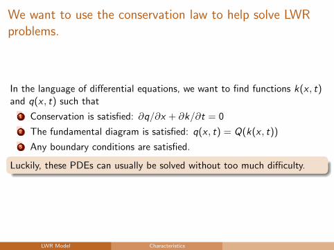
We want to use the conservation law to help solve LWRproblems.

In the language of differential equations, we want to find functions k(x , t)and q(x , t) such that

1 Conservation is satisfied: ∂q/∂x + ∂k/∂t = 0

2 The fundamental diagram is satisfied: q(x , t) = Q(k(x , t))

3 Any boundary conditions are satisfied.

Luckily, these PDEs can usually be solved without too much difficulty.

LWR Model Characteristics

The fundamental diagram implies that q is a function of k .

Therefore, the conservation law∂k

∂t+

∂q

∂x= 0 can be rewritten

∂k

∂t+

dq

dk

∂k

∂x= 0

which is a PDE in k(x , t) alone.

We can solve this PDE by looking for “characteristics,” curves along whichk(x , t) is constant.


∂k

∂t+

dq

dk

∂k

∂x= 0

In this model, the characteristics are straight lines. Consider a line with

slope dq/dk, so dx =dq

dkdt

If we move in this direction,

dk =∂k

∂tdt +

∂k

∂xdx

dk = −dq

dk

∂k

∂xdt +

∂k

∂x

dq

dkdt = 0

so k(x , t) is constant along a line with slope dq/dk. This is called thewave speed.


So, if I know the value of k(x , t) at any point (e.g., boundary condition), Iknow the value of k(x , t) at all points along the line through (x , t) withslope dq(x , t)/dk...unless there is “something else” which interferes (i.e., ashockwave).

In the “uncongested” portion of the fundamental diagram, dq/dk > 0, souncongested states propagate downstream.

In the “congested” portion of the fundamental diagram, dq/dk < 0, socongested states propagate upstream.

In other words, where there is no congestion, upstream conditions prevail.Where congestion exists, downstream conditions prevail.


NEWELL-DAGANZOMETHOD

The Newell-Daganzo method is an easier alternative tosolving the LWR model.

q

k

kj

uf -w

qmax

For now, assume a triangular fundamental diagram with only two wavespeeds: uf for the uncongested portion, and −w for the congested portion.

Notice that in a triangular fundamental diagram, speed does not drop untildensity exceeds the critical density and congestion sets in.

LWR Model Newell-Daganzo Method

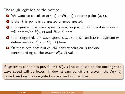
The rough logic behind the method:

1 We want to calculate k(x , t) or N(x , t) at some point (x , t).

2 Either this point is congested or uncongested.

3 If congested, the wave speed is −w , so past conditions downstreamwill determine k(x , t) and N(x , t) here.

4 If uncongested, the wave speed is uf , so past conditions upstream willdetermine k(x , t) and N(x , t) here.

5 Of these two possibilities, the correct solution is the onecorresponding to the lowest N(x , t) value.

If upstream conditions prevail, the N(x , t) value based on the uncongestedwave speed will be lower. If downstream conditions prevail, the N(x , t)value based on the congested wave speed will be lower.


The major tools in the Newell-Daganzo method:

1

N(x2, t2)− N(x1, t1) =

∫Cq dt − k dx

2 k (and therefore q) is constant along characteristics

3 Characteristics are straight lines, so q dt − k dx is constant, so theintegral is easy to evaluate.

4 With the simplified fundamental diagram, there are only twocharacteristic slopes possible


Change in vehicles along characteristic with positive slope

These characteristics reflect uncongested conditions, and have slope (wavespeed) uf .

∫Cq dt − k dx =

∫C

(q − k

dq

dk

)dt

dq/dk is the wave speed, uf .

However, uf is also the traffic speed for the uncongested case, so q = uf kand ∫

C

(q − k

dq

dk

)dt = 0

N(x , t) is constant along forward-moving characteristics. In other words,if you move with the speed of uncongested traffic, you should observe nochange in the cumulative vehicle count.


Change in vehicles along characteristic with negative slope

These characteristics reflect uncongested conditions, and have slope (wavespeed) −w .

∫Cq dt − k dx =

∫C

(q

dq/dk− k

)dx

dq/dk is the wave speed, −w .

∫Cq dt − k dx = −

∫C

(k + q/w) dx


From the fundamental diagram, k + q/w = kj

q

k

kj

uf -w

qmax

So ∫Cq dt − k dx = −

∫Ckjdx = kj(x2 − x1)

If you are moving at the backward wave speed, the cumulative vehicle countincreases at the rate of the jam density.


Example

A link is 1 mile long, and has free flow speed 30 mph, backward wavespeed 15 mph, and jam density 200 veh/mi. Vehicles enter upstream at arate of 1200 veh/hr. Three minutes from now, the downstream trafficsignal turns red. Four minutes from now, what is the cumulative countvalue at the midpoint of the link? Has the queue reached this point?


With a more general fundamental diagram, there are a larger number ofpossible characteristic speeds.

The problem then is to trace back all possible characteristics to a knownpoint (initial condition, boundary condition, previously-solved value),determine the change in vehicle number, and select the smallest.

This can be framed as a calculus of variations problem.


Documents

Lighthill-Whitham-Richards tra c ow model · Highway Capacity Manual Triangular: q = minfu f k;w(k j k)g Trapezoidal: q = minfu f k;q ... LWR Model Newell-Daganzo Method. With a more