LASER INTERFEROMETER GRAVITATIONAL WAVE OBSERVATORY

-LIGO-

CALIFORNIA INSTITUTE OF TECHNOLOGYMASSACHUSETTS INSTITUTE OF TECHNOLOGY

Technical Note LIGO-T000058- 00- R 5/11/2000

Measurement of Seismic Motion at 40mand transfer function of seismic stacks

D. Ugolini, S. Vass, A. Weinstein

This is an internal working noteof the LIGO Project.

California Institute of Technology Massachusetts Institute of Technology

LIGO Project - MS 18-34 LIGO Project - MS NW17-161

Pasadena CA 91125 Cambridge, MA 02139

Phone (626) 395-2129 Phone (617) 253-4824Fax (626) 304-9834 Fax (617) 253-4824

E-mail: info@ligo.caltech.edu E-mail: info@ligo.mit.eduWWW: http://www.ligo.caltech.edu/

�le /home/ajw/Docs/T000058-00.pdf

Dennis UgoliniSteve Vass

Alan WeinsteinLIGO Working Document

May 11, 2000DRAFT 0.94

Measurement of Seismic Motion at 40mand transfer function of seismic stacks

Abstract

In preparation for upgrading the Caltech 40m interferometer for protoyping LIGO II optical

con�gurations, we are measuring the seismic motion of the 40m laboratory and the transfer

function of the existing seismic stacks.

1 Introduction

We are attempting to measure the seismic noise and stack transfer functions at the 40m lab. Why?

� Well, just to understand it; learn how to do it, and compare with past measurements [1].

� To evaluate the need for active isolators (STACIS, IDE; we currently think it's a good idea).

� To validate our crude modelling of the stack transfer functions, in order to estimate whatthey'd be if we replaced the viton with damped metal springs (which we currently think isnot advisable).

Guided by the work reported in [2], We pursue two approaches:

� Use natural ground seismic motion, measure it on the oor and on top of a stack withseismometers, accelerometers, geophones, etc., reading out these instruments with the DAQSsystem, and analyzing the resulting frames with matlab.

� Use a shaker on the oor or on the stack support bars, and a spectrum analyzer in swept-sinemode to measure the transfer functions.

2 Measurements using natural ground seismic motion

Our equipment:

� We have obtained two 3-axis geophones from MIT (Barry Controls Triaxial MicrovelocitySensor). One is typically placed on the oor (in the frames, these signals are called \Floor-X", \Floor-Y", \Floor-Z"), and the other moves around (no matter where it is placed, in theframes, these signals are called \Stack-X", \Stack-Y", \Stack-Z").

1

� We have a 1-axis seismometer in the lab (in the frames, \IFO-Seis"), which we can orient anyway we want.

� We have a small audio microphone (in the frames, \Microphone").

These 8 signals are routed to 8 \spare" fast (16384 Hz) channels in the existing DAQ system, andcan be logged to the 40m RAID array when we want to take measurements.

The data are transferred by ftp to a big disk on canopus (a cpu server on the general ligo.caltech.edusun cluster) and are analyzed with matlab. We know of no way to run matlab on the 40m sun thathas the raid array (cdssol9 - albireo) or to mount the raid array on the general ligo.caltech.edu suncluster.

Calibration: The placard by the seismometer says 340 V/m/s, X20 for the preampli�er gain,for a total of 6800 V/(m/s). The geophone x- and y- coordinates are set to 1000 V/(in/sec) =39400 V/(m/s). The geophone z-coordinates are set to 100 V/(in/sec) = 3940 V/(m/s). The VMEfast ADC (a VMIC3123 16ch, 16-bit, 100kHz S/H ADC running at 16384 Hz) is set to 16384 adccounts / volt. So the �nal calibration constants are

� IFO-Seis: 1 ADC count = 9:0� 10�9 m/s

� Geophone x,y: 1 ADC count = 1:6 � 10�9 m/s

� Geophone z: 1 ADC count = 1:6� 10�8 m/s

� The microphone is in \arbitrary units"...

2.1 Analysis

� Read in to matlab, 64 seconds of data from all 8 channels, using frextract, a matlab functionto read frame data (from Benoit Mours' frame library, but only in version 3.71, for somereason). We had to modify frextract to close the frame �le.

� Apply calibration constants to the time series.

� Plot the seismometer time series; look for bumps to see if this is a quiet time.

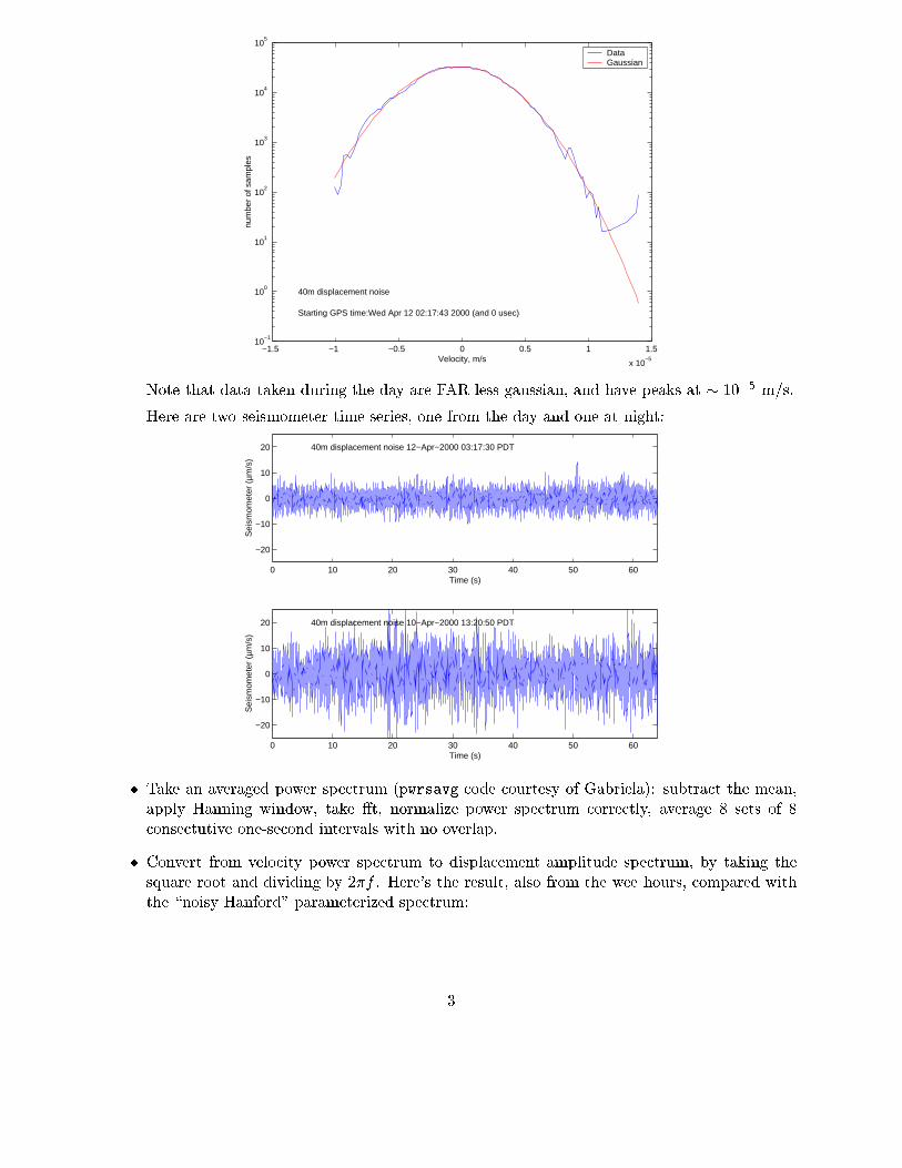
� Histogram the seismometer time series, and compare with a gaussian with the same meanand �, to look for non-gaussian seismic noise. Here's an example from the wee hours of thenight:

2

−1.5 −1 −0.5 0 0.5 1 1.5

x 10−5

10−1

100

101

102

103

104

105

Velocity, m/s

num

ber

of s

ampl

es

40m displacement noise

Starting GPS time:Wed Apr 12 02:17:43 2000 (and 0 usec)

Data Gaussian

Note that data taken during the day are FAR less gaussian, and have peaks at � 10�5 m/s.

Here are two seismometer time series, one from the day and one at night:

0 10 20 30 40 50 60

−20

−10

0

10

20

Time (s)

Sei

smom

eter

(µm

/s)

40m displacement noise 12−Apr−2000 03:17:30 PDT

0 10 20 30 40 50 60

−20

−10

0

10

20

Time (s)

Sei

smom

eter

(µm

/s)

40m displacement noise 10−Apr−2000 13:20:50 PDT

� Take an averaged power spectrum (pwrsavg code courtesy of Gabriela): subtract the mean,apply Hanning window, take �t, normalize power spectrum correctly, average 8 sets of 8consectutive one-second intervals with no overlap.

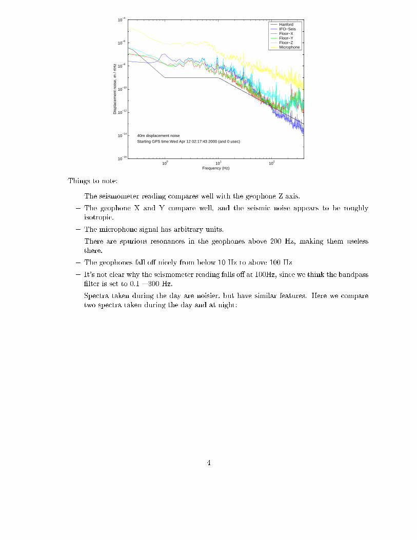
� Convert from velocity power spectrum to displacement amplitude spectrum, by taking thesquare root and dividing by 2�f . Here's the result, also from the wee hours, compared withthe \noisy Hanford" parameterized spectrum:

3

100

101

102

10−16

10−14

10−12

10−10

10−8

10−6

10−4

Frequency (Hz)

Dis

plac

emen

t noi

se, m

/ rt

Hz

40m displacement noise

Starting GPS time:Wed Apr 12 02:17:43 2000 (and 0 usec)

Hanford IFO−Seis Floor−X Floor−Y Floor−Z Microphone

Things to note:

{ The seismometer reading compares well with the geophone Z axis.

{ The geophone X and Y compare well, and the seismic noise appears to be roughlyisotropic.

{ The microphone signal has arbitrary units.

{ There are spurious resonances in the geophones above 200 Hz, making them uselessthere.

{ The geophones fall o� nicely from below 10 Hz to above 100 Hz

{ It's not clear why the seismometer reading falls o� at 100Hz, since we think the bandpass�lter is set to 0.1 { 300 Hz.

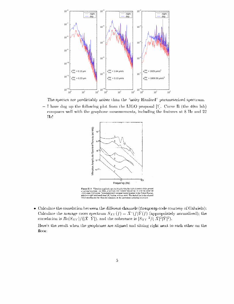
{ Spectra taken during the day are noisier, but have similar features. Here we comparetwo spectra taken during the day and at night:

4

100

101

102

10−12

10−11

10−10

10−9

10−8

10−7

10−6

zrmsnite = 0.13 µm

zrmsday = 0.23 µm

nightday

100

101

102

10−10

10−9

10−8

10−7

10−6

10−5

vrmsnite = 1.64 µm/s

vrmsday = 3.13 µm/s

nightday

100

101

102

10−8

10−7

10−6

10−5

10−4

10−3

armsnite = 1929 µm/s2

armsday = 1809.59 µm/s2

nightday

{ The spectra are predictably noiser than the \noisy Hanford" parameterized spectrum.

{ I have dug up the following plot from the LIGO proposal [1]. Curve B (the 40m lab)compares well with the geophone measurements, including the features at 8 Hz and 22Hz!

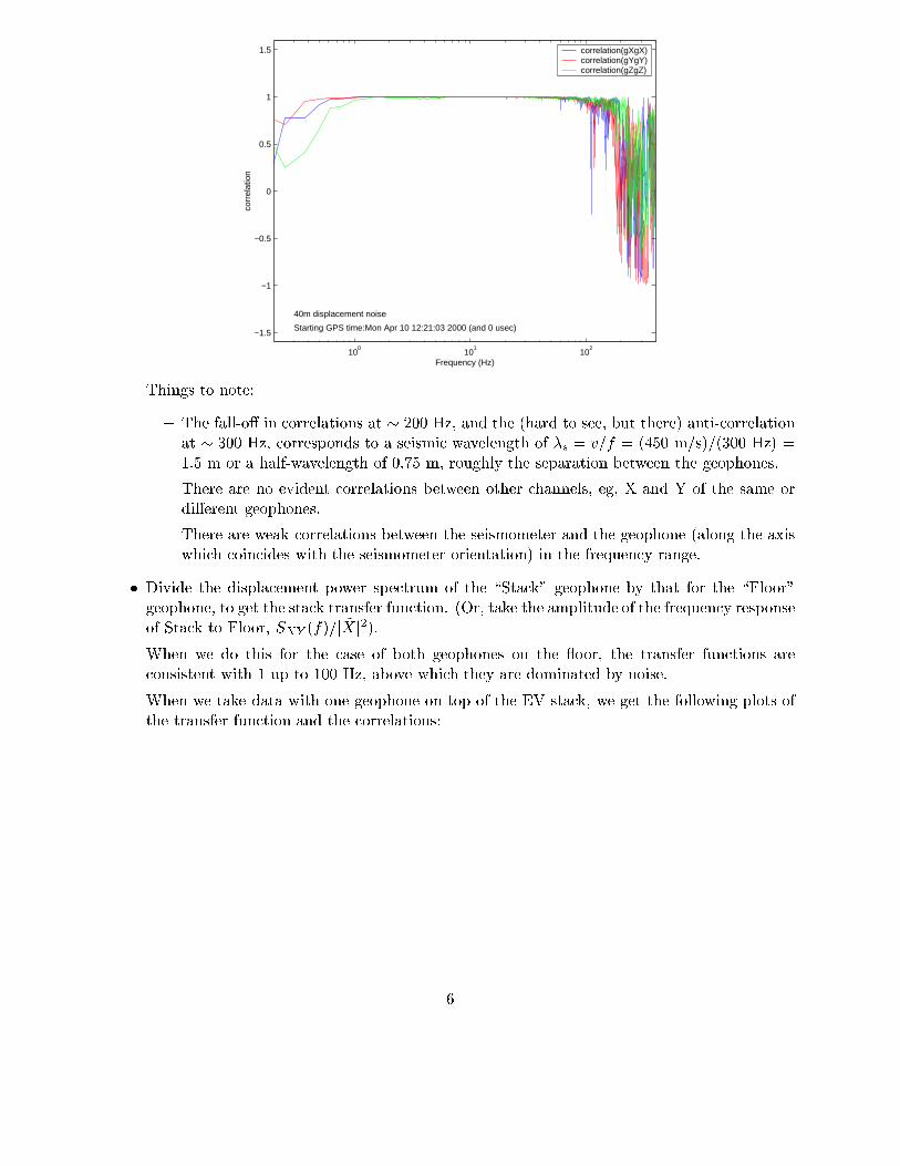
� Calculate the correlation between the di�erent channels (freqresp code courtesy of Gabriela):Calculate the average cross spectrum SXY (f) = ~X�(f) ~Y (f) (appropriately normalized); thecorrelation is Re(SXY )=(j ~X jj ~Y j), and the coherence is jSXY j2=(j ~X j2j ~Y j2).Here's the result when the geophones are aligned and sitting right next to each other on the oor:

5

100

101

102

−1.5

−1

−0.5

0

0.5

1

1.5

Frequency (Hz)

corr

elat

ion

40m displacement noise

Starting GPS time:Mon Apr 10 12:21:03 2000 (and 0 usec)

correlation(gXgX)correlation(gYgY)correlation(gZgZ)

Things to note:

{ The fall-o� in correlations at � 200 Hz, and the (hard to see, but there) anti-correlationat � 300 Hz, corresponds to a seismic wavelength of �s = v=f = (450 m/s)/(300 Hz) =1.5 m or a half-wavelength of 0.75 m, roughly the separation between the geophones.

{ There are no evident correlations between other channels, eg, X and Y of the same ordi�erent geophones.

{ There are weak correlations between the seismometer and the geophone (along the axiswhich coincides with the seismometer orientation) in the frequency range.

� Divide the displacement power spectrum of the \Stack" geophone by that for the \Floor"geophone, to get the stack transfer function. (Or, take the amplitude of the frequency responseof Stack to Floor, SXY (f)=j ~X j2).When we do this for the case of both geophones on the oor, the transfer functions areconsistent with 1 up to 100 Hz, above which they are dominated by noise.

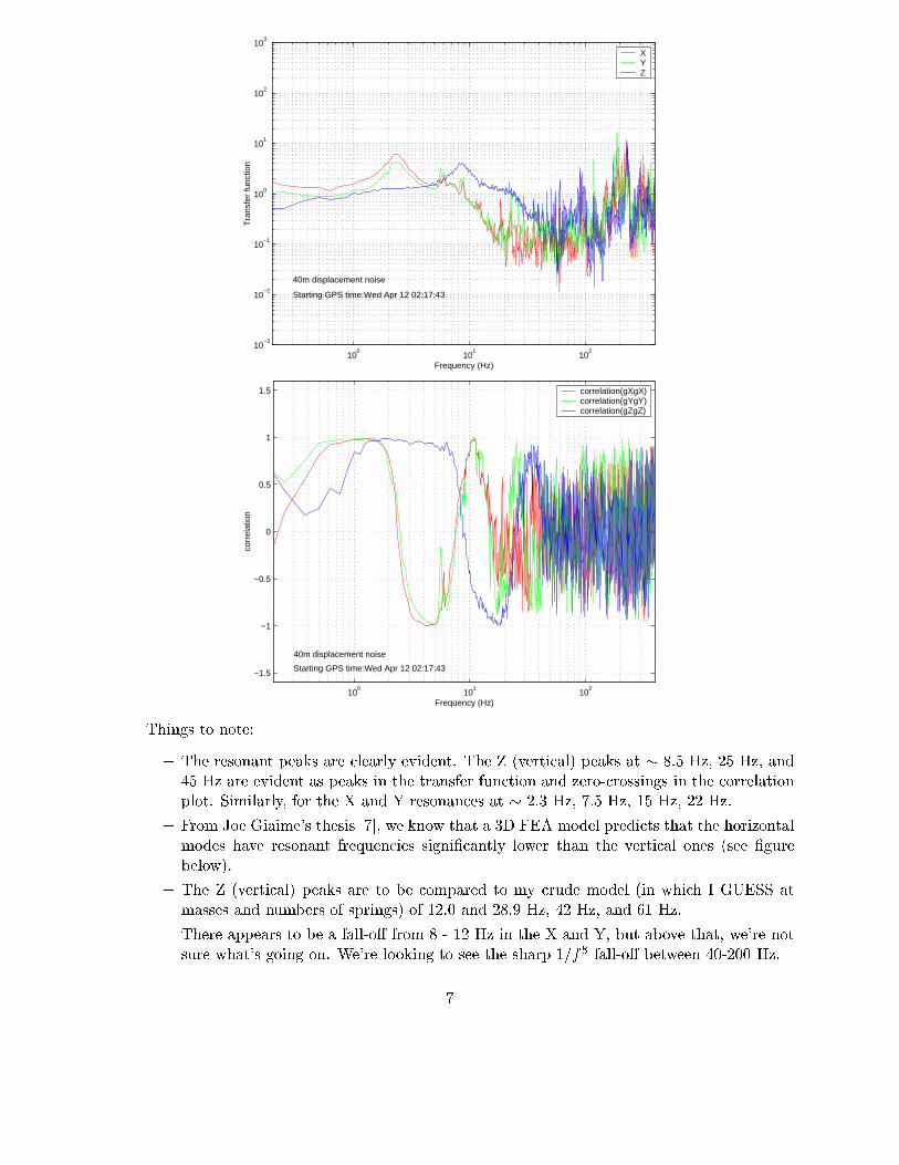
When we take data with one geophone on top of the EV stack, we get the following plots ofthe transfer function and the correlations:

6

100

101

102

10−3

10−2

10−1

100

101

102

103

Frequency (Hz)

Tra

nsfe

r fu

nctio

n

40m displacement noise

Starting GPS time:Wed Apr 12 02:17:43

XYZ

100

101

102

−1.5

−1

−0.5

0

0.5

1

1.5

Frequency (Hz)

corr

elat

ion

40m displacement noise

Starting GPS time:Wed Apr 12 02:17:43

correlation(gXgX)correlation(gYgY)correlation(gZgZ)

Things to note:

{ The resonant peaks are clearly evident. The Z (vertical) peaks at � 8.5 Hz, 25 Hz, and45 Hz are evident as peaks in the transfer function and zero-crossings in the correlationplot. Similarly, for the X and Y resonances at � 2.3 Hz, 7.5 Hz, 15 Hz, 22 Hz.

{ From Joe Giaime's thesis [7], we know that a 3D FEA model predicts that the horizontalmodes have resonant frequencies signi�cantly lower than the vertical ones (see �gurebelow).

{ The Z (vertical) peaks are to be compared to my crude model (in which I GUESS atmasses and numbers of springs) of 12.0 and 28.9 Hz, 42 Hz, and 61 Hz.

{ There appears to be a fall-o� from 8 - 12 Hz in the X and Y, but above that, we're notsure what's going on. We're looking to see the sharp 1=f8 fall-o� between 40-200 Hz.

7

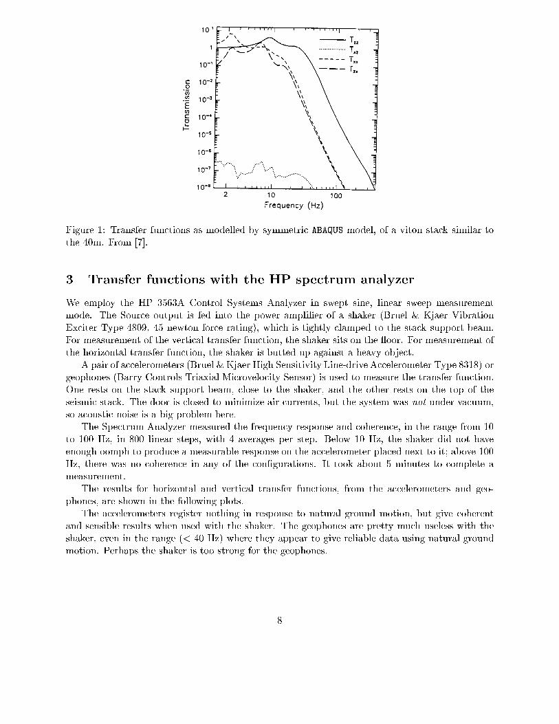
Figure 1: Transfer functions as modelled by symmetric ABAQUS model, of a viton stack similar tothe 40m. From [7].

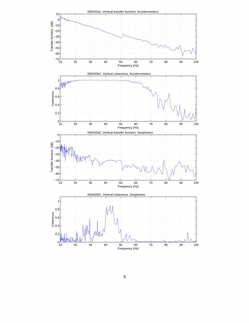
3 Transfer functions with the HP spectrum analyzer

We employ the HP 3563A Control Systems Analyzer in swept sine, linear sweep measurementmode. The Source output is fed into the power ampli�er of a shaker (Bruel & Kjaer VibrationExciter Type 4809, 45 newton force rating), which is tightly clamped to the stack support beam.For measurement of the vertical transfer function, the shaker sits on the oor. For measurement ofthe horizontal transfer function, the shaker is butted up against a heavy object.

A pair of accelerometers (Bruel & Kjaer High Sensitivity Line-drive Accelerometer Type 8318) orgeophones (Barry Controls Triaxial Microvelocity Sensor) is used to measure the transfer function.One rests on the stack support beam, close to the shaker, and the other rests on the top of theseismic stack. The door is closed to minimize air currents, but the system was not under vacuum,so acoustic noise is a big problem here.

The Spectrum Analyzer measured the frequency response and coherence, in the range from 10to 100 Hz, in 800 linear steps, with 4 averages per step. Below 10 Hz, the shaker did not haveenough oomph to produce a measurable response on the accelerometer placed next to it; above 100Hz, there was no coherence in any of the con�gurations. It took about 5 minutes to complete ameasurement.

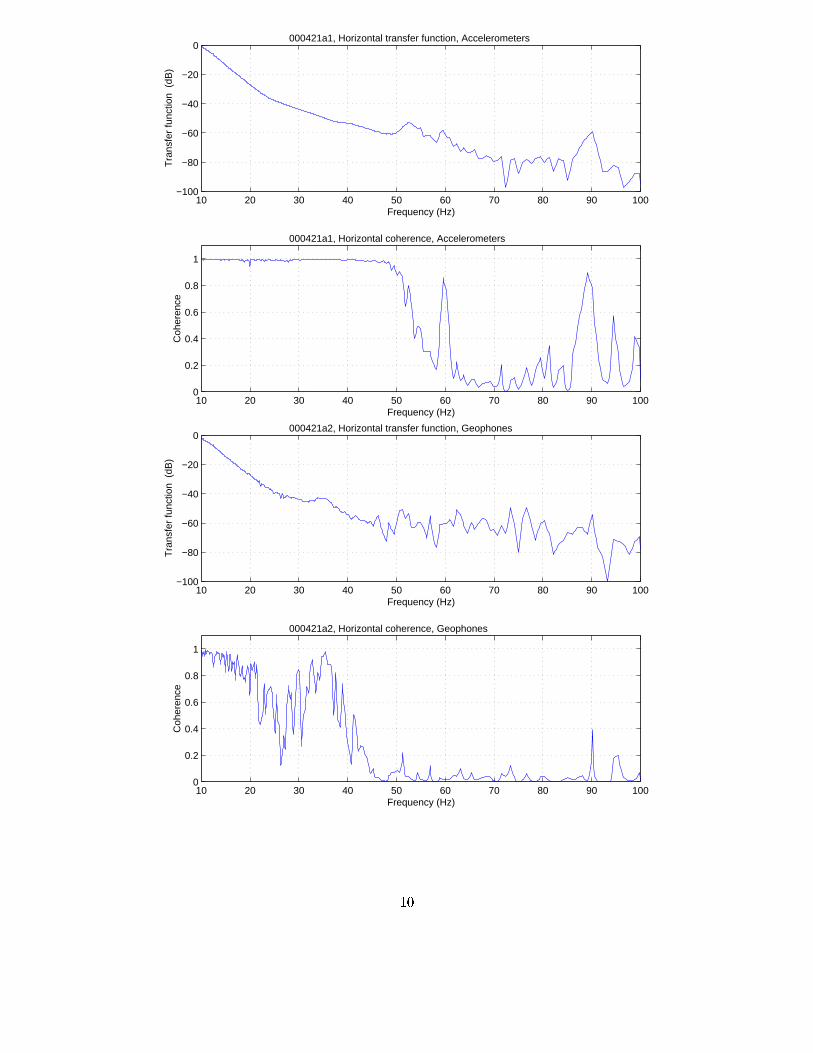
The results for horizontal and vertical transfer functions, from the accelerometers and geo-phones, are shown in the following plots.

The accelerometers register nothing in response to natural ground motion, but give coherentand sensible results when used with the shaker. The geophones are pretty much useless with theshaker, even in the range (< 40 Hz) where they appear to give reliable data using natural groundmotion. Perhaps the shaker is too strong for the geophones.

8

10 20 30 40 50 60 70 80 90 100−70

−60

−50

−40

−30

−20

−10

0

10000420a1, Vertical transfer function, Accelerometers

Tra

nsfe

r fu

nctio

n (

dB)

Frequency (Hz)

10 20 30 40 50 60 70 80 90 1000

0.2

0.4

0.6

0.8

1

000420b1, Vertical coherence, Accelerometers

Coh

eren

ce

Frequency (Hz)

10 20 30 40 50 60 70 80 90 100−70

−60

−50

−40

−30

−20

−10

0000420a2, Vertical transfer function, Geophones

Tra

nsfe

r fu

nctio

n (

dB)

Frequency (Hz)

10 20 30 40 50 60 70 80 90 1000

0.2

0.4

0.6

0.8

1

000420b2, Vertical coherence, Geophones

Coh

eren

ce

Frequency (Hz)

9

10 20 30 40 50 60 70 80 90 100−100

−80

−60

−40

−20

0000421a1, Horizontal transfer function, Accelerometers

Tra

nsfe

r fu

nctio

n (

dB)

Frequency (Hz)

10 20 30 40 50 60 70 80 90 1000

0.2

0.4

0.6

0.8

1

000421a1, Horizontal coherence, Accelerometers

Coh

eren

ce

Frequency (Hz)

10 20 30 40 50 60 70 80 90 100−100

−80

−60

−40

−20

0000421a2, Horizontal transfer function, Geophones

Tra

nsfe

r fu

nctio

n (

dB)

Frequency (Hz)

10 20 30 40 50 60 70 80 90 1000

0.2

0.4

0.6

0.8

1

000421a2, Horizontal coherence, Geophones

Coh

eren

ce

Frequency (Hz)

10

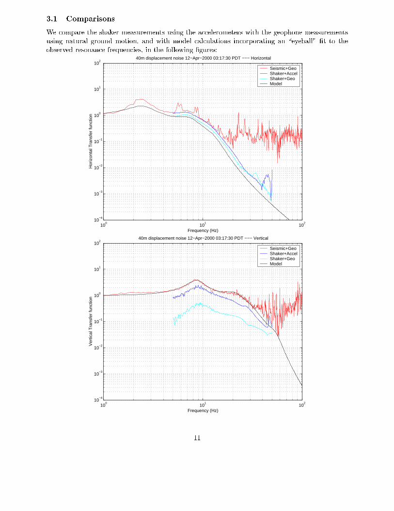
3.1 Comparisons

We compare the shaker measurements using the accelerometers with the geophone measurementsusing natural ground motion, and with model calculations incorporating an \eyeball" �t to theobserved resonance frequencies, in the following �gures:

100

101

102

10−4

10−3

10−2

10−1

100

101

102

Frequency (Hz)

Hor

izon

tal T

rans

fer

func

tion

40m displacement noise 12−Apr−2000 03:17:30 PDT −−− Horizontal

Seismic+Geo Shaker+AccelShaker+Geo Model

100

101

102

10−4

10−3

10−2

10−1

100

101

102

Frequency (Hz)

Ver

tical

Tra

nsfe

r fu

nctio

n

40m displacement noise 12−Apr−2000 03:17:30 PDT −−− Vertical

Seismic+Geo Shaker+AccelShaker+Geo Model

11

Things to note:

� The measured horizontal transfer functions compare well; in the range of overlap (between10 and 20 Hz), the shape of the transfer functions agree, and the levels agree to better thana factor 2...

� The vertical transfer functions agree in shape from 5 to 50 Hz, but the transfer function takenwith the shaker and accelerometers is a factor 2 below the transfer function taken with naturalground motion and geophones. (We measured no calibration o�set between the geophoneswhen they were placed next to each other). The one taken with the shaker and geophones islower still. This is not understood.

� The model of the vertical transfer function agrees well with the measurements made withgeophones and natural seismic motion, from 1 Hz to 50 Hz. It should fall like f�8 above 100Hz, but we don't know how to measure it there (without the interferometer).

� The model of the horizontal transfer function lies as much as a factor 2 below the data, butthe shape agrees in the range between 5 and 40 Hz.

� The model of the vertical transfer function has 4 poles, at 8.7, 21.0, 32.0, 55.0 Hz. The modelof the horizontal transfer function has 3 poles, at 2.5, 7.5, 13 Hz. Again, the models are justan eyeballing of the curves.

12

4 The currently existing stacks

At present, the 40m lab contains �ve seismic stacks with three legs and four stages, for the chambershousing the beam splitter (BS), south vertex (SV) test mass, south end (SE), east vertex (EV),and east end (EE). There is also an input optics chamber with a square optical table sitting on aone-leg, four stage stack. The layout can be seen in [3].

The three-legged stacks were installed in 4/93. The input optics chamber stack was built in1996, and installed at the end of that year[4] Engineering drawings for these stacks exist [5].

In each of these stacks, the masses are machined stainless steel, and the springs are vitonelastomer.

4.1 The transfer function

To quantify these issues at some level, we have made simple Matlab models of the vertical transferfunction

Tzz(f) =xtop(f)

xfloor(f)

for stacks consisting of all viton springs, all damped metal springs, and mixtures of springs. Foldlingthese in with the ground motion spectrum zfloor(f) allows us to predict the spectrum of motion atthe top of the stack, ztop(f), and calculate the integrated rms motion xrms and vz;rms.

4.2 Tzz versus Txz and Txx

For IFO locking and noise performance, the relevant motion is in the direction along the beam(x). However, the stacks are arranged vertically in the local gravitational �eld, and it is thereforeeasiest to model the vertical transfer function. The more relevant Tzx and Txx transfer functionscan only be reliably estimated using 3D �nite element analysis tools, which take into account themore complex couplings of z to x, and all the complex properties of all the materials, their shearmoduli and geometry, etc.

Fortunately, much work has already been done in this area, by Joe Giaime and others [7]. Assummarized in Fig. 1, we see that:

� Txz and Txx have seismic walls at frequencies typically a factor of 2 or more smaller than Tzz;

� If Tzz has a peak at 9 Hz, Txz and Txx peak in the 2 to 3 Hz region, and otherwise lie belowTzz.

� These predictions were con�rmed (qualitatively) with measurements of a test stack at MIT[7].

This �gure can be used to qualitatively extrapolate from a model of Tzz to the more relevantTxz and Txx.

4.3 The modelled transfer function

The stacks are designed and modelled as described in the appendix. Here we focus only on thethree-legged stacks housing the core optical components; the input and output chamber stacks havesimilar properties and less critical requirements.

13

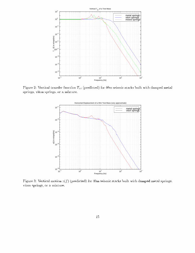
The vertical transfer function Tzz is shown in Fig. 2, and the vertical motion at the top of thestack, ztop(f), is shown in Fig. 3. In both �gures, we show the stacks with all viton springs, alldamped metal springs, and a mixture.

The features to note are:

� At high frequencies, all the stack transfer functions have the expected f�8 fallo�.

� The metal stacks have superior isolation at higher frequencies compared with the viton, withthe mixed stacks lying in between. The frequency at which the vertical displacement fallsbelow 1�18 m/

pHz is 39 Hz for metal and 91 Hz for viton.

� The metal stacks have resonant peaks that are less damped and at lower frequencies than theviton stacks, leading to higher peak motion at the resonant frequencies. The viton peaks areall but washed out by the damping.

The numbers used for the springs, all of which probably require con�rmation, are summarizedin table 1.

The numbers for the stacks are summarized in table 2. Analogous tables for LIGO stacks appearin Ref. [6], and we have checked our calculations against all the numbers in those tables.

14

10−1

100

101

102

103

10−14

10−12

10−10

10−8

10−6

10−4

10−2

100

102

Vertical Tzz

of a Test Mass

Frequency (hz)

Tzz

(f)

in m

/sqr

t(H

z)

metal springsviton springsmixed springs

Figure 2: Vertical transfer function Tzz (predicted) for 40m seismic stacks built with damped metalsprings, viton springs, or a mixture.

10−1

100

101

102

103

10−30

10−25

10−20

10−15

10−10

10−5

Horizontal Displacement of a 40m Test Mass (very approximate)

Frequency (hz)

x(f)

in m

/sqr

t(H

z)

metal springsviton springs

Figure 3: Vertical motion z(f) (predicted) for 40m seismic stacks built with damped metal springs,viton springs, or a mixture.

15

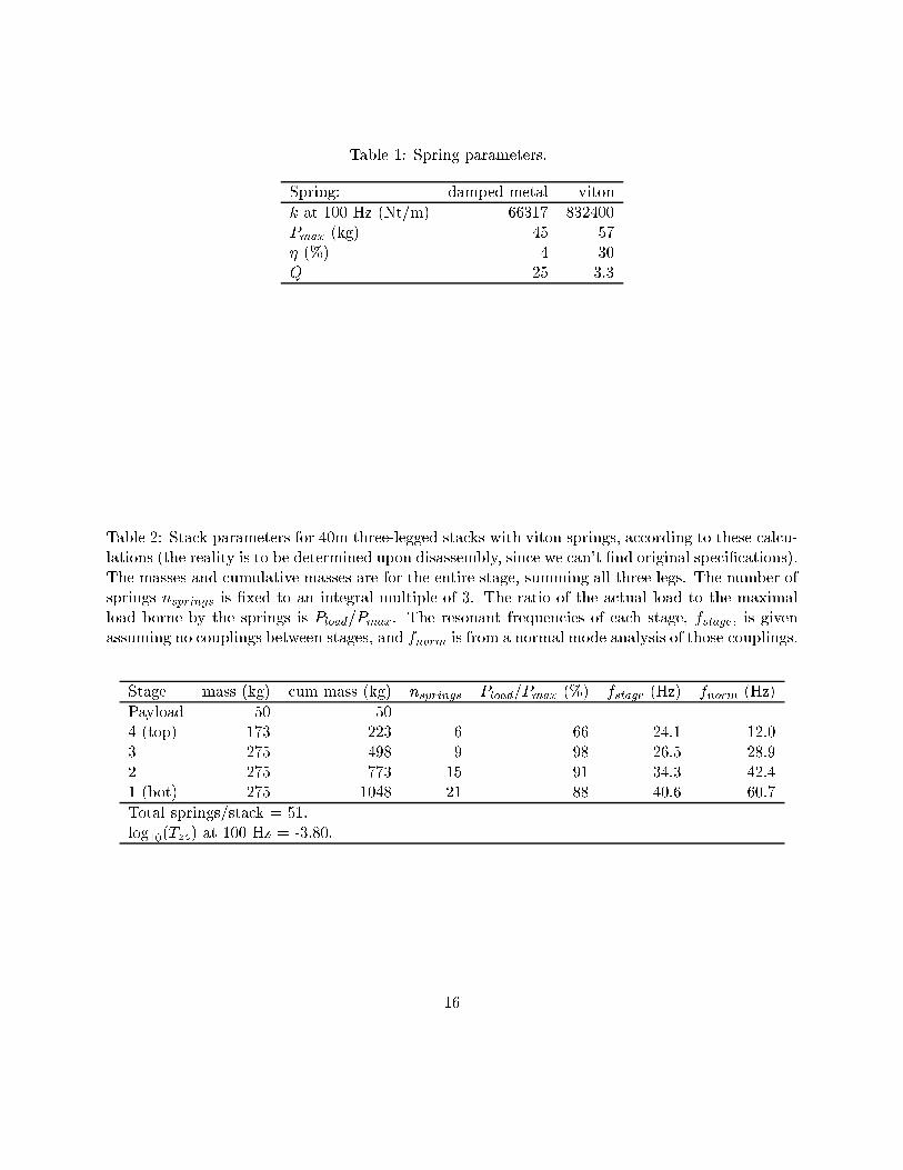
Table 1: Spring parameters.

Spring: damped metal viton

k at 100 Hz (Nt/m) 66317 832400Pmax (kg) 45 57� (%) 4 30Q 25 3.3

Table 2: Stack parameters for 40m three-legged stacks with viton springs, according to these calcu-lations (the reality is to be determined upon disassembly, since we can't �nd original speci�cations).The masses and cumulative masses are for the entire stage, summing all three legs. The number ofsprings nsprings is �xed to an integral multiple of 3. The ratio of the actual load to the maximalload borne by the springs is Pload=Pmax. The resonant frequencies of each stage, fstage, is givenassuming no couplings between stages, and fnorm is from a normal mode analysis of those couplings.

Stage mass (kg) cum mass (kg) nsprings Pload=Pmax (%) fstage (Hz) fnorm (Hz)

Payload 50 504 (top) 173 223 6 66 24.1 12.03 275 498 9 98 26.5 28.92 275 773 15 91 34.3 42.41 (bot) 275 1048 21 88 40.6 60.7

Total springs/stack = 51.log10(Tzz) at 100 Hz = -3.80.

16

5 Noise tolerance for lock acquisition

Lock acquisition depends primarily on the free-swinging velocity (distribution and rms) of themirror, hung from the suspension pendulum resting on the seismic stack.

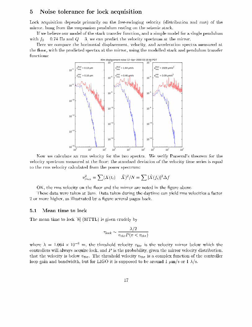
If we believe our model of the stack transfer function, and a simple model for a single pendulumwith f0 = 0:74 Hz and Q = 3, we can predict the velocity spectrum at the mirror.

Here we compare the horizontal displacement, velocity, and acceleration spectra measured atthe oor, with the predicted spectra at the mirror, using the modelled stack and pendulum transferfunctions:

100

101

102

10−16

10−14

10−12

10−10

10−8

10−6 z

rmsfloor = 0.13 µm

zrmsmirr = 0.16 µm

100

101

102

10−14

10−12

10−10

10−8

10−6

10−4

vrmsfloor = 1.64 µm/s

vrmsmirr = 0.46 µm/s

40m displacement noise 12−Apr−2000 03:18:44 PDT

100

101

102

10−12

10−10

10−8

10−6

10−4

10−2

armsfloor = 1929 µm/s2

armsmirr = 3.09 µm/s2

Now we calculate an rms velocity for the two spectra. We verify Parseval's theorem for thevelocity spectrum measured at the oor: the standard deviation of the velocity time series is equalto the rms velocity calculated from the power spectrum:

v2rms =X

(X(ti)� �X)2=N =X

j ~X(fi)j2�f

OK, the rms velocity on the oor and the mirror are noted in the �gure above.These data were taken at 3am. Data taken during the daytime can yield rms velocities a factor

2 or more higher, as illustrated by a �gure several pages back.

5.1 Mean time to lock

The mean time to lock [8] (MTTL) is given crudely by

�lock � �=2

vthrP (v < vthr)

where � = 1:064 � 10�6 m, the threshold velocity vthr is the velocity mirror below which thecontrollers will always acquire lock, and P is the probability, given the mirror velocity distribution,that the velocity is below vthr. The threshold velocity vthr is a complex function of the controllerloop gain and bandwidth, but for LIGO it is supposed to be around 1 �m/s or 1 �/s.

17

The rms velocity vrms of the mirror as estimated above is on the order of 1 �m/s or 1 �/s. Thiscompares well with The threshold velocity vthr, so that the mean time to lock is expected to be oforder 1s.

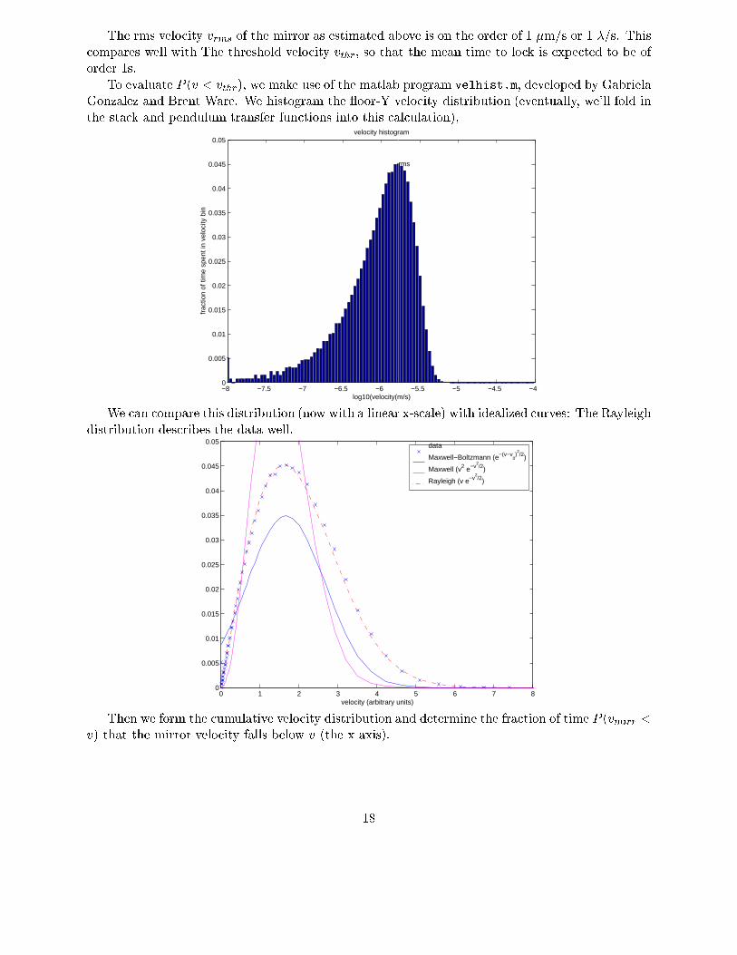
To evaluate P (v < vthr), we make use of the matlab program velhist.m, developed by GabrielaGonzalez and Brent Ware. We histogram the oor-Y velocity distribution (eventually, we'll fold inthe stack and pendulum transfer functions into this calculation),

−8 −7.5 −7 −6.5 −6 −5.5 −5 −4.5 −40

0.005

0.01

0.015

0.02

0.025

0.03

0.035

0.04

0.045

0.05

rms

log10(velocity(m/s)

frac

tion

of ti

me

spen

t in

velo

city

bin

velocity histogram

We can compare this distribution (now with a linear x-scale) with idealized curves: The Rayleighdistribution describes the data well.

0 1 2 3 4 5 6 7 80

0.005

0.01

0.015

0.02

0.025

0.03

0.035

0.04

0.045

0.05

velocity (arbitrary units)

data

Maxwell−Boltzmann (e−(v−v0)2/2)

Maxwell (v2 e−v2/2)

Rayleigh (v e−v2/2)

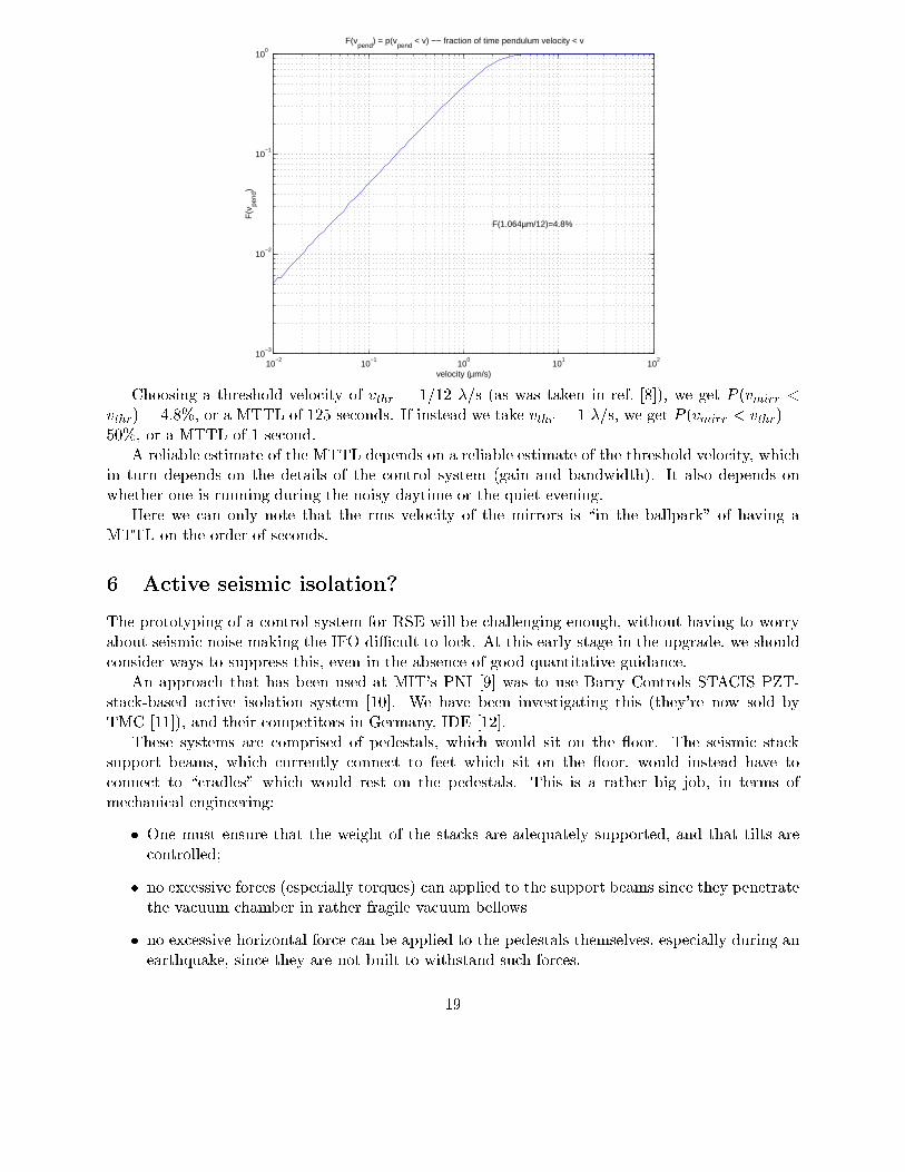
Then we form the cumulative velocity distribution and determine the fraction of time P (vmirr <v) that the mirror velocity falls below v (the x axis).

18

10−2

10−1

100

101

102

10−3

10−2

10−1

100

velocity (µm/s)

F(v

pend

)

F(vpend

) = p(vpend

< v) −− fraction of time pendulum velocity < v

F(1.064µm/12)=4.8%

Choosing a threshold velocity of vthr = 1/12 �/s (as was taken in ref. [8]), we get P (vmirr <vthr) = 4:8%, or a MTTL of 125 seconds. If instead we take vthr = 1 �/s, we get P (vmirr < vthr) =50%, or a MTTL of 1 second.

A reliable estimate of the MTTL depends on a reliable estimate of the threshold velocity, whichin turn depends on the details of the control system (gain and bandwidth). It also depends onwhether one is running during the noisy daytime or the quiet evening.

Here we can only note that the rms velocity of the mirrors is \in the ballpark" of having aMTTL on the order of seconds.

6 Active seismic isolation?

The prototyping of a control system for RSE will be challenging enough, without having to worryabout seismic noise making the IFO diÆcult to lock. At this early stage in the upgrade, we shouldconsider ways to suppress this, even in the absence of good quantitative guidance.

An approach that has been used at MIT's PNI [9] was to use Barry Controls STACIS PZT-stack-based active isolation system [10]. We have been investigating this (they're now sold byTMC [11]), and their competitors in Germany, IDE [12].

These systems are comprised of pedestals, which would sit on the oor. The seismic stacksupport beams, which currently connect to feet which sit on the oor, would instead have toconnect to \cradles" which would rest on the pedestals. This is a rather big job, in terms ofmechanical engineering:

� One must ensure that the weight of the stacks are adequately supported, and that tilts arecontrolled;

� no excessive forces (especially torques) can applied to the support beams since they penetratethe vacuum chamber in rather fragile vacuum bellows

� no excessive horizontal force can be applied to the pedestals themselves, especially during anearthquake, since they are not built to withstand such forces.

19

These systems are expensive: a pedestal costs in the neighborhood of $10K, and we need threefor each of 4 test mass stacks, for a total of 12.

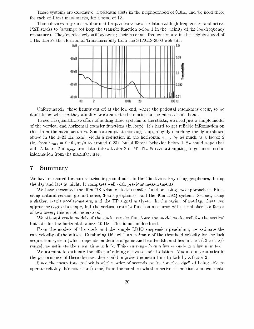
These devices rely on a rubber mat for passive vertical isolation at high frequencies, and activePZT stacks to (attempt to) keep the transfer function below 1 in the vicinity of the low-frequencyresonances. They're relatively sti� systems; their resonant frequencies are in the neighborhood of1 Hz. Here's the Horizontal Transmissibilty from the STACIS-2000 web site:

Unfortunately, these �gures cut o� at the low end, where the pedestal resonances occur, so wedon't know whether they amplify or attentuate the motion in the microseismic band.

To see the quantitative e�ect of adding these systems to the stacks, we need just a simple modelof the vertical and horizontal transfer functions (in loop). It's hard to get reliable information onthis, from the manufacturers. Some attempt at mocking it up, roughly matching the �gure shownabove in the 1{20 Hz band, yields a reduction in the horizontal vrms by as much as a factor 2(ie, from vrms = 0:46 �m/s to around 0.23), but di�erent behavior below 1 Hz could wipe thatout. A factor 2 in vrms translates into a factor 2 in MTTL. We are attempting to get more usefulinformation from the manufacturer.

7 Summary

We have measured the natural seismic ground noise in the 40m laboratory using geophones, duringthe day and late at night. It compares well with previous measurements.

We have measured the 40m BS seismic stack transfer function using two approaches: First,using natural seismic ground noise, 3-axis geophones, and the 40m DAQ system. Second, usinga shaker, 1-axis accelerometers, and the HP signal analyzer. In the region of overlap, these twoapproaches agree in shape, but the vertical transfer function measured with the shaker is a factorof two lower; this is not understood.

We attempt crude models of the stack transfer functions; the model works well for the verticalbut fails for the horizontal, above 10 Hz. This is not understood.

From the models of the stack and the simple LIGO suspension pendulum, we estimate therms velocity of the mirror. Combining this with an estimate of the threshold velocity for the lockacquisition system (which depends on details of gains and bandwidth, and lies in the 1/12 to 1 �/srange), we estimate the mean time to lock. This can range from a few seconds to a few minutes.

We attempt to estimate the e�ect of adding active seismic isolation. Modulo uncertainties inthe performance of these devices, they could improve the mean time to lock by a factor 2.

Since the mean time to lock is of the order of seconds, we're \on the edge" of being able tooperate reliably. It's not clear (to me) from the numbers whether active seismic isolation can make

20

the di�erence between easy and hard lock acquisition, and thus, whether it is worth the e�ort andexpense to implement it...

8 Acknowledgements

Many thanks to Gabriela Gonzalez, Fred Raab, Joe Giaime, Riccardo DeSalvo and his group, foradvice and help.

References

[1] LIGO Proposal to the NSF, LIGO-M890001-00-M.

[2] \Transfer function and drift measurements on the �rst-article HAM", M. Barton, J. Giaime,G. Gonzalez, W. Johnson, A. Marin. LIGO-T980084-00, 10/98.

[3] LIGO drawing D961304-06: http://www.ligo.caltech.edu/LIGO web/dcc/docs/D961304-06.pdf .

[4] LIGO note M960115-00, http://www.ligo.caltech.edu/LIGO web/dcc/docs/M960115-00.pdf .

[5] LIGO drawings 1205425-1205429, 1205431-1205433, 1205435-1205439, 1205441-1205452,1202092, 1101012.

[6] E. Ponslet, HYTEC-TN-LIGO-01 (1996); HYTEC-TN-LIGO-02 (1996); HYTEC-TN-LIGO-03 (1996); HYTEC-TN-LIGO-04a (1996); HYTEC-TN-LIGO-07a (1997);

[7] J. Giaime, PhD thesis, MIT (1995); J. Giaime, P. Saha, D. Shoemaker, and L. Sievers,Rev. Sci. Instrum. 67, 208-214 (1996).

[8] \The BIG BOOK of LIGO Lock Acquisition Design", B. Ware, LIGO-T-980666-00-D, 8/98.

[9] Partha Saha, Ph.D thesis, LIGO-P970012-00-R, MIT, February 1997.

[10] \Performance of the Barry Controls, Inc STACIS active isolation system", P. Fritschel andG. Gonzalez, LIGO-T950046-00-R, 1995.

[11] http://www.techmfg.com/Products/Advanced/STACIS2000.htm .

[12] http://www.ideworld.com/IDE/hauptindex.html .

21