Chapter 1Introduction to OpenGLChapter Objectives

After reading this chapter, you'll be able to do the following:

Appreciate in general terms what OpenGL offers  

Identify different levels of rendering complexity  

Understand the basic structure of an OpenGL program  

Recognize OpenGL command syntax  

Understand in general terms how to animate an OpenGL program

This chapter introduces OpenGL. It has the following major sections: "What Is OpenGL?" explains what OpenGL is, what it does and doesn't do, and how it works.  

"A Very Simple OpenGL Program" presents a small OpenGL program and briefly discusses it. This section also defines a few basic computer-graphics terms.  

"OpenGL Command Syntax" explains some of the conventions and notations used by OpenGL commands.  

"OpenGL as a State Machine" describes the use of state variables in OpenGL and the commands for querying, enabling, and disabling states.  

"OpenGL-related Libraries" describes sets of OpenGL-related routines, including an auxiliary library specifically written for this book to simplify programming

examples.  

"Animation" explains in general terms how to create pictures on the screen that move, or animate.

 

What Is OpenGL?OpenGL is a software interface to graphics hardware. This interface consists of about 120 distinct commands, which you use to specify the objects and operations needed to produce interactive three-dimensional applications.

OpenGL is designed to work efficiently even if the computer that displays the graphics you create isn't the computer that runs your graphics program. This might be the case if you work in a networked computer environment where many computers are connected to one another by wires capable of carrying digital data. In this situation, the computer on which your program runs and issues OpenGL drawing commands is called the client, and the computer that receives those commands and performs the drawing is called the server. The format for transmitting OpenGL commands (called the protocol) from the client to the server is always the same, so OpenGL programs can work across a network even if the client and server are different kinds of computers. If an OpenGL program isn't running across a network, then there's only one computer, and it is both the client and the server.

OpenGL is designed as a streamlined, hardware-independent interface to be implemented on many different hardware platforms. To achieve these qualities, no commands for performing windowing tasks or obtaining user input are included in OpenGL; instead, you must work through whatever windowing system controls the particular hardware you're using. Similarly, OpenGL doesn't provide high-level commands for describing models of three-dimensional objects. Such commands might allow you to specify relatively complicated shapes such as automobiles, parts of the body, airplanes, or molecules. With OpenGL, you must build up your desired model from a small set of geometric primitive - points, lines, and polygons. (A sophisticated library that provides these features could certainly be built on top of OpenGL - in fact, that's what Open Inventor is. See "OpenGL-related Libraries" for more information about Open Inventor.)

Now that you know what OpenGL doesn't do, here's what it does do. Take a look at the color plates - they illustrate typical uses of OpenGL. They show the scene on the cover of this book, drawn by a computer (which is to say, rendered) in successively more complicated ways. The following paragraphs describe in general terms how these pictures were made.

Figure J-1 shows the entire scene displayed as a wireframe model - that is, as if all the objects in the scene were made of wire. Each line of wire corresponds to an edge of a primitive (typically a polygon). For example, the surface of the table is constructed from triangular polygons that are positioned like slices of pie.

Note that you can see portions of objects that would be obscured if the objects were solid rather than wireframe. For example, you can see the entire model of the hills outside the window even though most of this model is normally hidden by the wall of the room. The globe appears to be nearly solid because it's composed of hundreds of colored blocks, and you see the wireframe lines for all the edges of all the blocks, even those forming the back side of the globe. The way the globe is constructed gives you an idea of how complex objects can be created by assembling lower-level objects.  

Figure J-2 shows a depth-cued version of the same wireframe scene. Note that the lines farther from the eye are dimmer, just as they would be in real life, thereby giving a visual cue of depth.  

Figure J-3 shows an antialiased version of the wireframe scene. Antialiasing is a technique for reducing the jagged effect created when only portions of neighboring pixels properly belong to the image being drawn. Such jaggies are usually the most visible with near-horizontal or near-vertical lines.  

Figure J-4 shows a flat-shaded version of the scene. The objects in the scene are now shown as solid objects of a single color. They appear "flat" in the sense that they don't seem to respond to the lighting conditions in the room, so they don't appear smoothly rounded.  

Figure J-5 shows a lit, smooth-shaded version of the scene. Note how the scene looks much more realistic and three-dimensional when the objects are shaded to respond to the light sources in the room; the surfaces of the objects now look smoothly rounded.  

Figure J-6 adds shadows and textures to the previous version of the scene. Shadows aren't an explicitly defined feature of OpenGL (there is no "shadow command"), but you can create them yourself using the techniques described in Chapter 13 . Texture mapping allows you to apply a two-dimensional texture to a three-dimensional object. In this scene, the top on the table surface is the most vibrant example of texture mapping. The walls, floor, table surface, and top (on top of the table) are all texture mapped.  

Figure J-7 shows a motion-blurred object in the scene. The sphinx (or dog, depending on your Rorschach tendencies) appears to be captured as it's moving forward, leaving a blurred trace of its path of motion.  

Figure J-8 shows the scene as it's drawn for the cover of the book from a different viewpoint. This plate illustrates that the image really is a snapshot of models of three-dimensional objects.

The next two color images illustrate yet more complicated visual effects that can be achieved with OpenGL:

Figure J-9 illustrates the use of atmospheric effects (collectively referred to as fog) to show the presence of particles in the air.  

Figure J-10 shows the depth-of-field effect, which simulates the inability of a camera lens to maintain all objects in a photographed scene in focus. The camera focuses on a particular spot in the scene, and objects that are significantly closer or farther than that spot are somewhat blurred.

The color plates give you an idea of the kinds of things you can do with the OpenGL graphics system. The next several paragraphs briefly describe the order in which OpenGL performs the major graphics operations necessary to render an image on the screen. Appendix A, "Order of Operations" describes this order of operations in more detail.

Construct shapes from geometric primitives, thereby creating mathematical descriptions of objects. (OpenGL considers points, lines, polygons, images, and bitmaps to be primitives.)  

Arrange the objects in three-dimensional space and select the desired vantage point for viewing the composed scene.  

Calculate the color of all the objects. The color might be explicitly assigned by the application, determined from specified lighting conditions, or obtained by pasting a texture onto the objects.  

Convert the mathematical description of objects and their associated color information to pixels on the screen. This process is called rasterization.

During these stages, OpenGL might perform other operations, such as eliminating parts of objects that are hidden by other objects (the hidden parts won't be drawn, which might increase performance). In addition, after the scene is rasterized but just before it's drawn on the screen, you can manipulate the pixel data if you want.

A Very Simple OpenGL ProgramBecause you can do so many things with the OpenGL graphics system, an OpenGL program can be complicated. However, the basic structure of a useful program can be simple: Its tasks are to initialize certain states that control how OpenGL renders and to specify objects to be rendered.

Before you look at an OpenGL program, let's go over a few terms. Rendering, which you've already seen used, is the process by which a computer creates images from models. These models, or objects, are constructed from geometric primitives - points, lines, and polygons - that are specified by their vertices.

The final rendered image consists of pixels drawn on the screen; a pixel - short for picture element - is the smallest visible element the display hardware can put on the screen. Information about the pixels (for instance, what color they're supposed to be) is organized in system memory into bitplanes. A bitplane is an area of memory that holds one bit of information for every pixel on the screen; the bit might indicate how red a particular pixel is supposed to be, for example. The bitplanes are themselves organized into a framebuffer, which holds all the information that the graphics display needs to control the intensity of all the pixels on the screen.

Now look at an OpenGL program. Example 1-1 renders a white rectangle on a black background, as shown in Figure 1-1 .

Figure 1-1 : A White Rectangle on a Black Background    

Example 1-1 : A Simple OpenGL Program

#include <whateverYouNeed.h>

main() {

   OpenAWindowPlease();

   glClearColor(0.0, 0.0, 0.0, 0.0);   glClear(GL_COLOR_BUFFER_BIT);   glColor3f(1.0, 1.0, 1.0);   glOrtho(-1.0, 1.0, -1.0, 1.0, -1.0, 1.0);    glBegin(GL_POLYGON);      glVertex2f(-0.5, -0.5);      glVertex2f(-0.5, 0.5);      glVertex2f(0.5, 0.5);      glVertex2f(0.5, -0.5);   glEnd();   glFlush();

   KeepTheWindowOnTheScreenForAWhile();}The first line of the main() routine opens a window on the screen: The OpenAWindowPlease() routine is meant as a placeholder for a window system-specific routine. The next two lines are OpenGL commands that clear the window to black: glClearColor() establishes what color the window will be cleared to, and glClear() actually clears the window. Once the color to clear to is set, the window is cleared to that color whenever glClear() is called. The clearing color can be changed with another call to glClearColor(). Similarly, the glColor3f() command establishes what color to use for drawing objects - in this case, the color is white. All objects drawn after this point use this color, until it's changed with another call to set the color.

The next OpenGL command used in the program, glOrtho(), specifies the coordinate system OpenGL assumes as it draws the final image and how the image gets mapped to the screen. The next calls, which are bracketed by glBegin() and glEnd(), define the object to be drawn - in this example, a polygon with four vertices. The polygon's "corners" are defined by the glVertex2f() commands. As you might be able to guess from the arguments, which are (x, y) coordinate pairs, the polygon is a rectangle.

Finally, glFlush() ensures that the drawing commands are actually executed, rather than stored in a buffer awaiting additional OpenGL commands. The KeepTheWindowOnTheScreenForAWhile() placeholder routine forces the picture to remain on the screen instead of immediately disappearing.

OpenGL Command SyntaxAs you might have observed from the simple program in the previous section, OpenGL commands use the prefix gl and initial capital letters for each word making up the command name (recall glClearColor(), for example). Similarly, OpenGL defined

constants begin with GL_, use all capital letters, and use underscores to separate words (like GL_COLOR_BUFFER_BIT).

You might also have noticed some seemingly extraneous letters appended to some command names (the 3f in glColor3f(), for example). It's true that the Color part of the command name is enough to define the command as one that sets the current color. However, more than one such command has been defined so that you can use different types of arguments. In particular, the 3 part of the suffix indicates that three arguments are given; another version of the Color command takes four arguments. The f part of the suffix indicates that the arguments are floating-point numbers. Some OpenGL commands accept as many as eight different data types for their arguments. The letters used as suffixes to specify these data types for ANSI C implementations of OpenGL are shown in Table 1-1 , along with the corresponding OpenGL type definitions. The particular implementation of OpenGL that you're using might not follow this scheme exactly; an implementation in C++ or Ada, for example, wouldn't need to.

Table 1-1 : Command Suffixes and Argument Data Types

Suffix Data Type Typical Corresponding C-Language Type

OpenGL Type Definition

b 8-bit integer signed char GLbyte

s 16-bit integer short GLshort

i 32-bit integer long GLint, GLsizei

f 32-bit floating-point

float GLfloat, GLclampf

d 64-bit floating-point

double GLdouble, GLclampd

ub 8-bit unsigned integer

unsigned char GLubyte, GLboolean

us 16-bit unsigned integer

unsigned short GLushort

ui 32-bit unsigned integer

unsigned long GLuint, GLenum, GLbitfield

 

Thus, the two commands

glVertex2i(1, 3);glVertex2f(1.0, 3.0);are equivalent, except that the first specifies the vertex's coordinates as 32-bit integers and the second specifies them as single-precision floating-point numbers.

Some OpenGL commands can take a final letter v, which indicates that the command takes a pointer to a vector (or array) of values rather than a series of individual arguments. Many commands have both vector and nonvector versions, but some commands accept only individual arguments and others require that at least some of the arguments be specified as a vector. The following lines show how you might use a vector and a nonvector version of the command that sets the current color:

glColor3f(1.0, 0.0, 0.0);

float color_array[] = {1.0, 0.0, 0.0};glColor3fv(color_array);In the rest of this guide (except in actual code examples), OpenGL commands are referred to by their base names only, and an asterisk is included to indicate that there may be more to the command name. For example, glColor*() stands for all variations of the command you use to set the current color. If we want to make a specific point about one version of a particular command, we include the suffix necessary to define that version. For example, glVertex*v() refers to all the vector versions of the command you use to specify vertices.

Finally, OpenGL defines the constant GLvoid; if you're programming in C, you can use this instead of void.

OpenGL as a State MachineOpenGL is a state machine. You put it into various states (or modes) that then remain in effect until you change them. As you've already seen, the current color is a state variable. You can set the current color to white, red, or any other color, and thereafter every object is drawn with that color until you set the current color to something else. The current color is only one of many state variables that OpenGL preserves. Others control such things as the current viewing and projection transformations, line and polygon stipple patterns, polygon drawing modes, pixel-packing conventions, positions and characteristics of lights, and material properties of the objects being drawn. Many state variables refer to modes that are enabled or disabled with the command glEnable() or glDisable().

Each state variable or mode has a default value, and at any point you can query the system for each variable's current value. Typically, you use one of the four following commands to do this: glGetBooleanv(), glGetDoublev(), glGetFloatv(), or glGetIntegerv(). Which of these commands you select depends on what data type you want the answer to be given in. Some state variables have a more specific query command (such as glGetLight*(), glGetError(), or glGetPolygonStipple()). In addition, you can save and later restore the values of a collection of state variables on an attribute stack with the glPushAttrib() and glPopAttrib() commands. Whenever possible, you should use these commands rather than any of the query commands, since they're likely to be more efficient.

The complete list of state variables you can query is found in Appendix B . For each variable, the appendix also lists the glGet*() command that returns the variable's value, the attribute class to which it belongs, and the variable's default value.

OpenGL-related LibrariesOpenGL provides a powerful but primitive set of rendering commands, and all higher-level drawing must be done in terms of these commands. Therefore, you might want to write your own library on top of OpenGL to simplify your programming tasks. Also, you might want to write some routines that allow an OpenGL program to work easily with your windowing system. In fact, several such libraries and routines have already been written to provide specialized features, as follows. Note that the first two libraries are provided with every OpenGL implementation, the third was written for this book and is available using ftp, and the fourth is a separate product that's based on OpenGL.

The OpenGL Utility Library (GLU) contains several routines that use lower-level OpenGL commands to perform such tasks as setting up matrices for specific viewing orientations and projections, performing polygon tessellation, and rendering surfaces. This library is provided as part of your OpenGL implementation. It's described in more detail in Appendix C and in the OpenGL Reference Manual. The more useful GLU routines are described in the chapters in this guide, where they're relevant to the topic being discussed. GLU routines use the prefix glu.  

The OpenGL Extension to the X Window System (GLX) provides a means of creating an OpenGL context and associating it with a drawable window on a machine that uses the X Window System. GLX is provided as an adjunct to OpenGL. It's described in more detail in both Appendix D and the OpenGL Reference Manual. One of the GLX routines (for swapping framebuffers) is described in "Animation." GLX routines use the prefix glX.  

The OpenGL Programming Guide Auxiliary Library was written specifically for this book to make programming examples simpler and yet more complete. It's the subject of the next section, and it's described in more detail in Appendix E . Auxiliary library routines use the prefix aux. "How to Obtain the Sample Code" describes how to obtain the source code for the auxiliary library.  

Open Inventor is an object-oriented toolkit based on OpenGL that provides objects and methods for creating interactive three-dimensional graphics applications. Available from Silicon Graphics and written in C++, Open Inventor provides pre-built objects and a built-in event model for user interaction, high-level application components for creating and editing three-dimensional scenes, and the ability to print objects and exchange data in other graphics formats.

The OpenGL Programming Guide Auxiliary Library

As you know, OpenGL contains rendering commands but is designed to be independent of any window system or operating system. Consequently, it contains no commands for opening windows or reading events from the keyboard or mouse. Unfortunately, it's impossible to write a complete graphics program without at least opening a window, and most interesting programs require a bit of user input or other services from the operating system or window system. In many cases, complete programs make the most interesting examples, so this book uses a small auxiliary library to simplify opening windows, detecting input, and so on.

In addition, since OpenGL's drawing commands are limited to those that generate simple geometric primitives (points, lines, and polygons), the auxiliary library includes several routines that create more complicated three-dimensional objects such as a sphere, a torus, and a teapot. This way, snapshots of program output can be interesting to look at. If you have an implementation of OpenGL and this auxiliary library on your system, the examples in this book should run without change when linked with them.

The auxiliary library is intentionally simple, and it would be difficult to build a large application on top of it. It's intended solely to support the examples in this book, but you may find it a useful starting point to begin building real applications. The rest of this section briefly describes the auxiliary library routines so that you can follow the programming examples in the rest of this book. Turn to Appendix E for more details about these routines.

Window Management

Three routines perform tasks necessary to initialize and open a window: auxInitWindow() opens a window on the screen. It enables the Escape key to be used to exit the program, and it sets the background color for the window to black.  

auxInitPosition() tells auxInitWindow() where to position a window on the screen.  

auxInitDisplayMode() tells auxInitWindow() whether to create an RGBA or color-index window. You can also specify a single- or double-buffered window. (If you're working in color-index mode, you'll want to load certain colors into the color map; use auxSetOneColor() to do this.) Finally, you can use this routine to indicate that you want the window to have an associated depth, stencil, and/or accumulation buffer.

Handling Input Events

You can use these routines to register callback commands that are invoked when specified events occur.

auxReshapeFunc() indicates what action should be taken when the window is resized, moved, or exposed.  

auxKeyFunc() and auxMouseFunc() allow you to link a keyboard key or a mouse button with a routine that's invoked when the key or mouse button is pressed or released.

Drawing 3-D Objects

The auxiliary library includes several routines for drawing these three-dimensional objects:

sphere octahedron

cube dodecahedron

torus icosahedron

cylinder teapot

cone

You can draw these objects as wireframes or as solid shaded objects with surface normals defined. For example, the routines for a sphere and a torus are as follows:

void auxWireSphere(GLdouble radius);

void auxSolidSphere(GLdouble radius);

void auxWireTorus(GLdouble innerRadius, GLdouble outerRadius);

void auxSolidTorus(GLdouble innerRadius, GLdouble outerRadius);

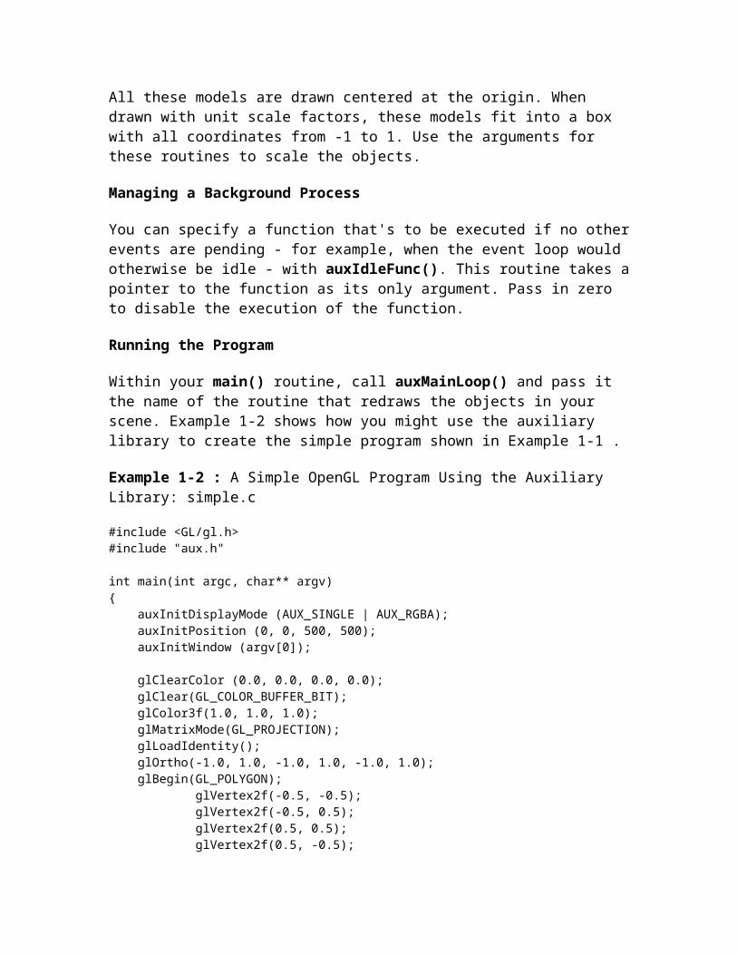
All these models are drawn centered at the origin. When drawn with unit scale factors, these models fit into a box with all coordinates from -1 to 1. Use the arguments for these routines to scale the objects.

Managing a Background Process

You can specify a function that's to be executed if no other events are pending - for example, when the event loop would otherwise be idle - with auxIdleFunc(). This routine takes a pointer to the function as its only argument. Pass in zero to disable the execution of the function.

Running the Program

Within your main() routine, call auxMainLoop() and pass it the name of the routine that redraws the objects in your scene. Example 1-2 shows how you might use the auxiliary library to create the simple program shown in Example 1-1 .

Example 1-2 : A Simple OpenGL Program Using the Auxiliary Library: simple.c

#include <GL/gl.h>#include "aux.h"

int main(int argc, char** argv){    auxInitDisplayMode (AUX_SINGLE | AUX_RGBA);    auxInitPosition (0, 0, 500, 500);    auxInitWindow (argv[0]);

    glClearColor (0.0, 0.0, 0.0, 0.0);    glClear(GL_COLOR_BUFFER_BIT);    glColor3f(1.0, 1.0, 1.0);    glMatrixMode(GL_PROJECTION);    glLoadIdentity();    glOrtho(-1.0, 1.0, -1.0, 1.0, -1.0, 1.0);    glBegin(GL_POLYGON);            glVertex2f(-0.5, -0.5);            glVertex2f(-0.5, 0.5);            glVertex2f(0.5, 0.5);            glVertex2f(0.5, -0.5);    glEnd();    glFlush();

    sleep(10);}

Animation

One of the most exciting things you can do on a graphics computer is draw pictures that move. Whether you're an engineer trying to see all sides of a mechanical part you're designing, a pilot learning to fly an airplane using a simulation, or merely a computer-game aficionado, it's clear that animation is an important part of computer graphics.

In a movie theater, motion is achieved by taking a sequence of pictures (24 per second), and then projecting them at 24 per second on the screen. Each frame is moved into position behind the lens, the shutter is opened, and the frame is displayed. The shutter is momentarily closed while the film is advanced to the next frame, then that frame is displayed, and so on. Although you're watching 24 different frames each second, your brain blends them all into a smooth animation. (The old Charlie Chaplin movies were shot at 16 frames per second and are noticeably jerky.) In fact, most modern projectors display each picture twice at a rate of 48 per second to reduce flickering. Computer-graphics screens typically refresh (redraw the picture) approximately 60 to 76 times per second, and some even run at about 120 refreshes per second. Clearly, 60 per second is smoother than 30, and 120 is marginally better than 60. Refresh rates faster than 120, however, are beyond the point of diminishing returns, since the human eye is only so good.

The key idea that makes motion picture projection work is that when it is displayed, each frame is complete. Suppose you try to do computer animation of your million-frame movie with a program like this:

open_window(); for (i = 0; i < 1000000; i++) {    clear_the_window();    draw_frame(i);    wait_until_a_24th_of_a_second_is_over(); }If you add the time it takes for your system to clear the screen and to draw a typical frame, this program gives more and more disturbing results depending on how close to 1/24 second it takes to clear and draw. Suppose the drawing takes nearly a full 1/24 second. Items drawn first are visible for the full 1/24 second and present a solid image on the screen; items drawn toward the end are instantly cleared as the program starts on the next frame, so they present at best a ghostlike image, since for most of the 1/24 second your eye is viewing the cleared background instead of the items that were unlucky enough to be drawn last. The problem is that this program doesn't display completely drawn frames; instead, you watch the drawing as it happens.

An easy solution is to provide double-buffering - hardware or software that supplies two complete color buffers. One is displayed while the other is being drawn. When the drawing of a frame is complete, the two buffers are swapped, so the one that was being viewed is now used for drawing, and vice versa. It's like a movie projector with only two frames in a loop; while one is being projected on the screen, an artist is desperately erasing and redrawing the frame that's not visible. As long as the artist is quick enough, the viewer notices no difference between this setup and one where all the frames are already drawn and the projector is simply displaying them one after the other. With

double-buffering, every frame is shown only when the drawing is complete; the viewer never sees a partially drawn frame.

A modified version of the preceding program that does display smoothly animated graphics might look like this:

open_window_in_double_buffer_mode(); for (i = 0; i < 1000000; i++) {    clear_the_window();    draw_frame(i);    swap_the_buffers(); }In addition to simply swapping the viewable and drawable buffers, the swap_the_buffers() routine waits until the current screen refresh period is over so that the previous buffer is completely displayed. This routine also allows the new buffer to be completely displayed, starting from the beginning. Assuming that your system refreshes the display 60 times per second, this means that the fastest frame rate you can achieve is 60 frames per second, and if all your frames can be cleared and drawn in under 1/60 second, your animation will run smoothly at that rate.

What often happens on such a system is that the frame is too complicated to draw in 1/60 second, so each frame is displayed more than once. If, for example, it takes 1/45 second to draw a frame, you get 30 frames per second, and the graphics are idle for 1/30-1/45=1/90 second per frame. Although 1/90 second of wasted time might not sound bad, it's wasted each 1/30 second, so actually one-third of the time is wasted.

In addition, the video refresh rate is constant, which can have some unexpected performance consequences. For example, with the 1/60 second per refresh monitor and a constant frame rate, you can run at 60 frames per second, 30 frames per second, 20 per second, 15 per second, 12 per second, and so on (60/1, 60/2, 60/3, 60/4, 60/5, ...). That means that if you're writing an application and gradually adding features (say it's a flight simulator, and you're adding ground scenery), at first each feature you add has no effect on the overall performance - you still get 60 frames per second. Then, all of a sudden, you add one new feature, and your performance is cut in half because the system can't quite draw the whole thing in 1/60 of a second, so it misses the first possible buffer-swapping time. A similar thing happens when the drawing time per frame is more than 1/30 second - the performance drops from 30 to 20 frames per second, giving a 33 percent performance hit.

Another problem is that if the scene's complexity is close to any of the magic times (1/60 second, 2/60 second, 3/60 second, and so on in this example), then because of random variation, some frames go slightly over the time and some slightly under, and the frame rate is irregular, which can be visually disturbing. In this case, if you can't simplify the scene so that all the frames are fast enough, it might be better to add an intentional tiny delay to make sure they all miss, giving a constant, slower, frame rate. If your frames have drastically different complexities, a more sophisticated approach might be necessary.

Interestingly, the structure of real animation programs does not differ too much from this description. Usually, the entire buffer is redrawn from scratch for each frame, as it is easier to do this than to figure out what parts require redrawing. This is especially true with applications such as three-dimensional flight simulators where a tiny change in the plane's orientation changes the position of everything outside the window.

In most animations, the objects in a scene are simply redrawn with different transformations - the viewpoint of the viewer moves, or a car moves down the road a bit, or an object is rotated slightly. If significant modifications to a structure are being made for each frame where there's significant recomputation, the attainable frame rate often slows down. Keep in mind, however, that the idle time after the swap_the_buffers() routine can often be used for such calculations.

OpenGL doesn't have a swap_the_buffers() command because the feature might not be available on all hardware and, in any case, it's highly dependent on the window system. However, GLX provides such a command, for use on machines that use the X Window System:

void glXSwapBuffers(Display *dpy, Window window);Example 1-3 illustrates the use of glXSwapBuffers() in an example that draws a square that rotates constantly, as shown in Figure 1-2 .

Figure 1-2 : A Double-Buffered Rotating Square    

Example 1-3 : A Double-Buffered Program: double.c

#include <GL/gl.h>#include <GL/glu.h>#include <GL/glx.h>#include "aux.h"

static GLfloat spin = 0.0;

void display(void){

    glClear(GL_COLOR_BUFFER_BIT);    glPushMatrix();    glRotatef(spin, 0.0, 0.0, 1.0);    glRectf(-25.0, -25.0, 25.0, 25.0);    glPopMatrix();

    glFlush();    glXSwapBuffers(auxXDisplay(), auxXWindow());}

void spinDisplay(void){    spin = spin + 2.0;    if (spin > 360.0)        spin = spin - 360.0;    display();}

void startIdleFunc(AUX_EVENTREC *event){    auxIdleFunc(spinDisplay);}

void stopIdleFunc(AUX_EVENTREC *event){    auxIdleFunc(0);}

void myinit(void){    glClearColor(0.0, 0.0, 0.0, 1.0);    glColor3f(1.0, 1.0, 1.0);    glShadeModel(GL_FLAT);}

void myReshape(GLsizei w, GLsizei h){    glViewport(0, 0, w, h);    glMatrixMode(GL_PROJECTION);    glLoadIdentity();    if (w <= h)         glOrtho (-50.0, 50.0, -50.0*(GLfloat)h/(GLfloat)w,             50.0*(GLfloat)h/(GLfloat)w, -1.0, 1.0);    else         glOrtho (-50.0*(GLfloat)w/(GLfloat)h,             50.0*(GLfloat)w/(GLfloat)h, -50.0, 50.0, -1.0, 1.0);    glMatrixMode(GL_MODELVIEW);    glLoadIdentity ();}

int main(int argc, char** argv){    auxInitDisplayMode(AUX_DOUBLE | AUX_RGBA);    auxInitPosition(0, 0, 500, 500);    auxInitWindow(argv[0]);    myinit();

    auxReshapeFunc(myReshape);    auxIdleFunc(spinDisplay);    auxMouseFunc(AUX_LEFTBUTTON, AUX_MOUSEDOWN, startIdleFunc);    auxMouseFunc(AUX_MIDDLEBUTTON, AUX_MOUSEDOWN, stopIdleFunc);    auxMainLoop(display);}

[Previous chapter] [Next chapter]

See the About page for copyright, authoring and distribution information.

Chapter 2Drawing Geometric ObjectsChapter Objectives

After reading this chapter, you'll be able to do the following:

Clear the window to an arbitrary color  

Draw with any geometric primitive - points, lines, and polygons - in two or three dimensions  

Control the display of those primitives - for example, draw dashed lines or outlined polygons  

Specify normal vectors at appropriate points on the surface of solid objects  

Force any pending drawing to complete

Although you can draw complex and interesting pictures using OpenGL, they're all constructed from a small number of primitive graphical items. This shouldn't be too surprising - look at what Leonardo da Vinci accomplished with just pencils and paintbrushes.

At the highest level of abstraction, there are three basic drawing operations: clearing the window, drawing a geometric object, and drawing a raster object. Raster objects, which include such things as two-dimensional images, bitmaps, and character fonts, are covered in Chapter 8 . In this chapter, you learn how to clear the screen and to draw geometric objects, including points, straight lines, and flat polygons.

You might think to yourself, "Wait a minute. I've seen lots of computer graphics in movies and on television, and there are plenty of beautifully shaded curved lines and surfaces. How are those drawn, if all OpenGL can draw are straight lines and flat polygons?" Even the image on the cover of this book includes a round table and objects on the table that have curved surfaces. It turns out that all the curved lines and surfaces you've seen are approximated by large numbers of little flat polygons or straight lines, in

much the same way that the globe on the cover is constructed from a large set of rectangular blocks. The globe doesn't appear to have a smooth surface because the blocks are relatively large compared to the globe. Later in this chapter, we show you how to construct curved lines and surfaces from lots of small geometric primitives.

This chapter has the following major sections:

"A Drawing Survival Kit" explains how to clear the window and force drawing to be completed. It also gives you basic information about controlling the color of geometric objects and about hidden-surface removal.  

"Describing Points, Lines, and Polygons" shows you what the set of primitive geometric objects is and how to draw them.  

"Displaying Points, Lines, and Polygons" explains what control you have over the details of how primitives are drawn - for example, what diameter points have, whether lines are solid or dashed, and whether polygons are outlined or filled.  

"Normal Vectors" discusses how to specify normal vectors for geometric objects and (briefly) what these vectors are for.  

"Some Hints for Building Polygonal Models of Surfaces" explores the issues and techniques involved in constructing polygonal approximations to surfaces.

One thing to keep in mind as you read the rest of this chapter is that with OpenGL, unless you specify otherwise, every time you issue a drawing command, the specified object is drawn. This might seem obvious, but in some systems, you first make a list of things to draw, and when it's complete, you tell the graphics hardware to draw the items in the list. The first style is called immediate-mode graphics and is OpenGL's default style. In addition to using immediate mode, you can choose to save some commands in a list (called a display list) for later drawing. Immediate-mode graphics is typically easier to program, but display lists are often more efficient. Chapter 4 tells you how to use display lists and why you might want to use them.

A Drawing Survival KitThis section explains how to clear the window in preparation for drawing, set the color of objects that are to be drawn, and force drawing to be completed. None of these subjects has anything to do with geometric objects in a direct way, but any program that draws geometric objects has to deal with these issues. This section also introduces the concept of hidden-surface removal, a technique that can be used to draw geometric objects easily.

Clearing the Window

Drawing on a computer screen is different from drawing on paper in that the paper starts out white, and all you have to do is draw the picture. On a computer, the memory holding the picture is usually filled with the last picture you drew, so you typically need to clear it to some background color before you start to draw the new scene. The color you use for the background depends on the application. For a word processor, you might clear to white (the color of the paper) before you begin to draw the text. If you're drawing a view from a spaceship, you clear to the black of space before beginning to draw the stars, planets, and alien spaceships. Sometimes you might not need to clear the screen at all; for example, if the image is the inside of a room, the entire graphics window gets covered as you draw all the walls.

At this point, you might be wondering why we keep talking about clearing the window - why not just draw a rectangle of the appropriate color that's large enough to cover the entire window? First, a special command to clear a window can be much more efficient than a general-purpose drawing command. In addition, as you'll see in Chapter 3 , OpenGL allows you to set the coordinate system, viewing position, and viewing direction arbitrarily, so it might be difficult to figure out an appropriate size and location for a window-clearing rectangle. Also, you can have OpenGL use hidden-surface removal techniques that eliminate objects obscured by others nearer to the eye; thus, if the window-clearing rectangle is to be a background, you must make sure that it's behind all the other objects of interest. With an arbitrary coordinate system and point of view, this might be difficult. Finally, on many machines, the graphics hardware consists of multiple buffers in addition to the buffer containing colors of the pixels that are displayed. These other buffers must be cleared from time to time, and it's convenient to have a single command that can clear any combination of them. (All the possible buffers are discussed in Chapter 10 .)

As an example, these lines of code clear the window to black:

glClearColor(0.0, 0.0, 0.0, 0.0); glClear(GL_COLOR_BUFFER_BIT);The first line sets the clearing color to black, and the next command clears the entire window to the current clearing color. The single parameter to glClear() indicates which buffers are to be cleared. In this case, the program clears only the color buffer, where the image displayed on the screen is kept. Typically, you set the clearing color once, early in your application, and then you clear the buffers as often as necessary. OpenGL keeps track of the current clearing color as a state variable rather than requiring you to specify it each time a buffer is cleared.

Chapter 5 and Chapter 10 talk about how other buffers are used. For now, all you need to know is that clearing them is simple. For example, to clear both the color buffer and the depth buffer, you would use the following sequence of commands:

glClearColor(0.0, 0.0, 0.0, 0.0); glClearDepth(0.0); 

glClear(GL_COLOR_BUFFER_BIT | GL_DEPTH_BUFFER_BIT);In this case, the call to glClearColor() is the same as before, the glClearDepth() command specifies the value to which every pixel of the depth buffer is to be set, and the parameter to the glClear() command now consists of the logical OR of all the buffers to be cleared. The following summary of glClear() includes a table that lists the buffers that can be cleared, their names, and the chapter where each type of buffer is discussed.void glClearColor(GLclampf red, GLclampf green, GLclampf blue, GLclampf alpha);

Sets the current clearing color for use in clearing color buffers in RGBA mode. For more information on RGBA mode, see Chapter 5 . The red, green, blue, and alpha values are clamped if necessary to the range [0,1]. The default clearing color is (0, 0, 0, 0), which is black.

void glClear(GLbitfield mask);

Clears the specified buffers to their current clearing values. The mask argument is a bitwise-ORed combination of the values listed in Table 2-1 .

Table 2-1 : Clearing Buffers

Buffer Name Reference

Color buffer GL_COLOR_BUFFER_BIT Chapter 5

Depth buffer GL_DEPTH_BUFFER_BIT Chapter 10

Accumulation buffer GL_ACCUM_BUFFER_BIT Chapter 10

Stencil buffer GL_STENCIL_BUFFER_BIT Chapter 10

 

Before issuing a command to clear multiple buffers, you have to set the values to which each buffer is to be cleared if you want something other than the default color, depth value, accumulation color, and stencil index. In addition to the glClearColor() and glClearDepth() commands that set the current values for clearing the color and depth buffers, glClearIndex(), glClearAccum(), and glClearStencil() specify the color index, accumulation color, and stencil index used to clear the corresponding buffers. See Chapter 5 and Chapter 10 for descriptions of these buffers and their uses.

OpenGL allows you to specify multiple buffers because clearing is generally a slow operation, since every pixel in the window (possibly millions) is touched, and some

graphics hardware allows sets of buffers to be cleared simultaneously. Hardware that doesn't support simultaneous clears performs them sequentially. The difference between

glClear(GL_COLOR_BUFFER_BIT | GL_DEPTH_BUFFER_BIT);and glClear(GL_COLOR_BUFFER_BIT); glClear(GL_DEPTH_BUFFER_BIT);is that although both have the same final effect, the first example might run faster on many machines. It certainly won't run more slowly.

Specifying a Color

With OpenGL, the description of the shape of an object being drawn is independent of the description of its color. Whenever a particular geometric object is drawn, it's drawn using the currently specified coloring scheme. The coloring scheme might be as simple as "draw everything in fire-engine red," or might be as complicated as "assume the object is made out of blue plastic, that there's a yellow spotlight pointed in such and such a direction, and that there's a general low-level reddish-brown light everywhere else." In general, an OpenGL programmer first sets the color or coloring scheme, and then draws the objects. Until the color or coloring scheme is changed, all objects are drawn in that color or using that coloring scheme. This method helps OpenGL achieve higher drawing performance than would result if it didn't keep track of the current color.

For example, the pseudocode

set_current_color(red); draw_object(A); draw_object(B); set_current_color(green); set_current_color(blue); draw_object(C);draws objects A and B in red, and object C in blue. The command on the fourth line that sets the current color to green is wasted.

Coloring, lighting, and shading are all large topics with entire chapters or large sections devoted to them. To draw geometric primitives that can be seen, however, you need some basic knowledge of how to set the current color; this information is provided in the next paragraphs. For details on these topics, see Chapter 5 and Chapter 6 .

To set a color, use the command glColor3f(). It takes three parameters, all of which are floating-point numbers between 0.0 and 1.0. The parameters are, in order, the red, green, and blue components of the color. You can think of these three values as specifying a "mix" of colors: 0.0 means don't use any of that component, and 1.0 means use all you can of that component. Thus, the code

glColor3f(1.0, 0.0, 0.0);makes the brightest red the system can draw, with no green or blue components. All zeros makes black; in contrast, all ones makes white. Setting all three components to 0.5 yields

gray (halfway between black and white). Here are eight commands and the colors they would set: glColor3f(0.0, 0.0, 0.0);                             black glColor3f(1.0, 0.0, 0.0);                             red glColor3f(0.0, 1.0, 0.0);                             green glColor3f(1.0, 1.0, 0.0);                             yellow glColor3f(0.0, 0.0, 1.0);                             blue glColor3f(1.0, 0.0, 1.0);                             magenta glColor3f(0.0, 1.0, 1.0);                             cyan glColor3f(1.0, 1.0, 1.0);                             whiteYou might have noticed earlier that when you're setting the color to clear the color buffer, glClearColor() takes four parameters, the first three of which match the parameters for glColor3f(). The fourth parameter is the alpha value; it's covered in detail in "Blending." For now, always set the fourth parameter to 0.0.

Forcing Completion of Drawing

Most modern graphics systems can be thought of as an assembly line, sometimes called a graphics pipeline. The main central processing unit (CPU) issues a drawing command, perhaps other hardware does geometric transformations, clipping occurs, then shading or texturing is performed, and finally, the values are written into the bitplanes for display (see Appendix A for details on the order of operations). In high-end architectures, each of these operations is performed by a different piece of hardware that's been designed to perform its particular task quickly. In such an architecture, there's no need for the CPU to wait for each drawing command to complete before issuing the next one. While the CPU is sending a vertex down the pipeline, the transformation hardware is working on transforming the last one sent, the one before that is being clipped, and so on. In such a system, if the CPU waited for each command to complete before issuing the next, there could be a huge performance penalty.

In addition, the application might be running on more than one machine. For example, suppose that the main program is running elsewhere (on a machine called the client), and that you're viewing the results of the drawing on your workstation or terminal (the server), which is connected by a network to the client. In that case, it might be horribly inefficient to send each command over the network one at a time, since considerable overhead is often associated with each network transmission. Usually, the client gathers a collection of commands into a single network packet before sending it. Unfortunately, the network code on the client typically has no way of knowing that the graphics program is finished drawing a frame or scene. In the worst case, it waits forever for enough additional drawing commands to fill a packet, and you never see the completed drawing.

For this reason, OpenGL provides the command glFlush(), which forces the client to send the network packet even though it might not be full. Where there is no network and all commands are truly executed immediately on the server, glFlush() might have no effect. However, if you're writing a program that you want to work properly both with and without a network, include a call to glFlush() at the end of each frame or scene. Note that glFlush() doesn't wait for the drawing to complete - it just forces the drawing to

begin execution, thereby guaranteeing that all previous commands execute in finite time even if no further rendering commands are executed.

A few commands - for example, commands that swap buffers in double-buffer mode - automatically flush pending commands onto the network before they can occur. void glFlush(void);

Forces previously issued OpenGL commands to begin execution, thus guaranteeing that they complete in finite time.

If glFlush() isn't sufficient for you, try glFinish(). This command flushes the network as glFlush() does and then waits for notification from the graphics hardware or network indicating that the drawing is complete in the framebuffer. You might need to use glFinish() if you want to synchronize tasks - for example, to make sure that your three-dimensional rendering is on the screen before you use Display PostScript to draw labels on top of the rendering. Another example would be to ensure that the drawing is complete before it begins to accept user input. After you issue a glFinish() command, your graphics process is blocked until it receives notification from the graphics hardware (or client, if you're running over a network) that the drawing is complete. Keep in mind that excessive use of glFinish() can reduce the performance of your application, especially if you're running over a network, because it requires round-trip communication. If glFlush() is sufficient for your needs, use it instead of glFinish().void glFinish(void);

Forces all previously issued OpenGL commands to complete. This command doesn't return until all effects from previous commands are fully realized.

Hidden-Surface Removal Survival Kit

When you draw a scene composed of three-dimensional objects, some of them might obscure all or parts of others. Changing your viewpoint can change the obscuring relationship. For example, if you view the scene from the opposite direction, any object that was previously in front of another is now behind it. To draw a realistic scene, these obscuring relationships must be maintained. If your code works something like this while (1) {    get_viewing_point_from_mouse_position();    glClear(GL_COLOR_BUFFER_BIT);    draw_3d_object_A();    draw_3d_object_B(); }it might be that for some mouse positions, object A obscures object B, and for others, the opposite relationship might hold. If nothing special is done, the preceding code always draws object B second, and thus on top of object A, no matter what viewing position is selected.

The elimination of parts of solid objects that are obscured by others is called hidden-surface removal. (Hidden-line removal, which does the same job for objects represented as wireframe skeletons, is a bit trickier, and it isn't discussed here. See "Hidden-Line

Removal," for details.) The easiest way to achieve hidden-surface removal is to use the depth buffer (sometimes called a z-buffer). (Also see Chapter 10 .)

A depth buffer works by associating a depth, or distance from the viewpoint, with each pixel on the window. Initially, the depth values for all pixels are set to the largest possible distance using the glClear() command with GL_DEPTH_BUFFER_BIT, and then the objects in the scene are drawn in any order.

Graphical calculations in hardware or software convert each surface that's drawn to a set of pixels on the window where the surface will appear if it isn't obscured by something else. In addition, the distance from the eye is computed. With depth buffering enabled, before each pixel is drawn, a comparison is done with the depth value already stored at the pixel. If the new pixel is closer to the eye than what's there, the new pixel's color and depth values replace those that are currently written into the pixel. If the new pixel's depth is greater than what's currently there, the new pixel would be obscured, and the color and depth information for the incoming pixel is discarded. Since information is discarded rather than used for drawing, hidden-surface removal can increase your performance.

To use depth buffering, you need to enable depth buffering. This has to be done only once. Each time you draw the scene, before drawing you need to clear the depth buffer and then draw the objects in the scene in any order.

To convert the preceding program fragment so that it performs hidden-surface removal, modify it to the following:

glEnable(GL_DEPTH_TEST); ... while (1) {    glClear(GL_COLOR_BUFFER_BIT | GL_DEPTH_BUFFER_BIT);    get_viewing_point_from_mouse_position();    draw_3d_object_A();    draw_3d_object_B(); }The argument to glClear() clears both the depth and color buffers.

Describing Points, Lines, and PolygonsThis section explains how to describe OpenGL geometric primitives. All geometric primitives are eventually described in terms of their vertices - coordinates that define the points themselves, the endpoints of line segments, or the corners of polygons. The next section discusses how these primitives are displayed and what control you have over their display.

What Are Points, Lines, and Polygons?

You probably have a fairly good idea of what a mathematician means by the terms point, line, and polygon. The OpenGL meanings aren't quite the same, however, and it's important to understand the differences. The differences arise because mathematicians can think in a geometrically perfect world, whereas the rest of us have to deal with real-world limitations.

For example, one difference comes from the limitations of computer-based calculations. In any OpenGL implementation, floating-point calculations are of finite precision, and they have round-off errors. Consequently, the coordinates of OpenGL points, lines, and polygons suffer from the same problems.

Another difference arises from the limitations of a bitmapped graphics display. On such a display, the smallest displayable unit is a pixel, and although pixels might be less than 1/100th of an inch wide, they are still much larger than the mathematician's infinitely small (for points) or infinitely thin (for lines). When OpenGL performs calculations, it assumes points are represented as vectors of floating-point numbers. However, a point is typically (but not always) drawn as a single pixel, and many different points with slightly different coordinates could be drawn by OpenGL on the same pixel.

Points

A point is represented by a set of floating-point numbers called a vertex. All internal calculations are done as if vertices are three-dimensional. Vertices specified by the user as two-dimensional (that is, with only x and y coordinates) are assigned a z coordinate equal to zero by OpenGL.

Advanced

OpenGL works in the homogeneous coordinates of three-dimensional projective geometry, so for internal calculations, all vertices are represented with four floating-point coordinates (x, y, z, w). If w is different from zero, these coordinates correspond to the euclidean three-dimensional point (x/w, y/w, z/w). You can specify the w coordinate in OpenGL commands, but that's rarely done. If the w coordinate isn't specified, it's understood to be 1.0. For more information about homogeneous coordinate systems, see Appendix G .

Lines

In OpenGL, line means line segment, not the mathematician's version that extends to infinity in both directions. There are easy ways to specify a connected series of line segments, or even a closed, connected series of segments (see Figure 2-1 ). In all cases, though, the lines comprising the connected series are specified in terms of the vertices at their endpoints.

Figure 2-1 : Two Connected Series of Line Segments    

Polygons

Polygons are the areas enclosed by single closed loops of line segments, where the line segments are specified by the vertices at their endpoints. Polygons are typically drawn with the pixels in the interior filled in, but you can also draw them as outlines or a set of points, as described in "Polygon Details."

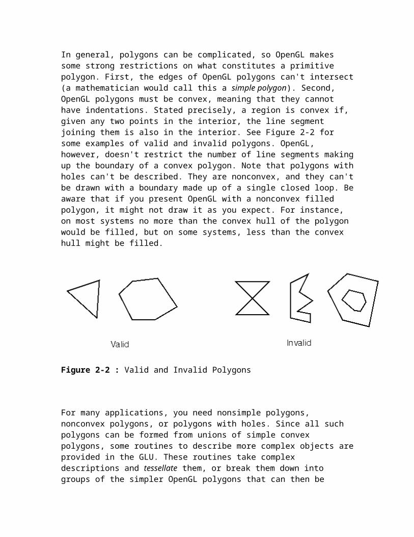
In general, polygons can be complicated, so OpenGL makes some strong restrictions on what constitutes a primitive polygon. First, the edges of OpenGL polygons can't intersect (a mathematician would call this a simple polygon). Second, OpenGL polygons must be convex, meaning that they cannot have indentations. Stated precisely, a region is convex if, given any two points in the interior, the line segment joining them is also in the interior. See Figure 2-2 for some examples of valid and invalid polygons. OpenGL, however, doesn't restrict the number of line segments making up the boundary of a convex polygon. Note that polygons with holes can't be described. They are nonconvex, and they can't be drawn with a boundary made up of a single closed loop. Be aware that if you present OpenGL with a nonconvex filled polygon, it might not draw it as you expect. For instance, on most systems no more than the convex hull of the polygon would be filled, but on some systems, less than the convex hull might be filled.

Figure 2-2 : Valid and Invalid Polygons    

For many applications, you need nonsimple polygons, nonconvex polygons, or polygons with holes. Since all such polygons can be formed from unions of simple convex polygons, some routines to describe more complex objects are provided in the GLU. These routines take complex descriptions and tessellate them, or break them down into groups of the simpler OpenGL polygons that can then be rendered. (See Appendix C for more information about the tessellation routines.) The reason for OpenGL's restrictions on valid polygon types is that it's simpler to provide fast polygon-rendering hardware for that restricted class of polygons.

Since OpenGL vertices are always three-dimensional, the points forming the boundary of a particular polygon don't necessarily lie on the same plane in space. (Of course, they do in many cases - if all the z coordinates are zero, for example, or if the polygon is a triangle.) If a polygon's vertices don't lie in the same plane, then after various rotations in space, changes in the viewpoint, and projection onto the display screen, the points might no longer form a simple convex polygon. For example, imagine a four-point quadrilateral where the points are slightly out of plane, and look at it almost edge-on. You can get a nonsimple polygon that resembles a bow tie, as shown in Figure 2-3 , which isn't guaranteed to render correctly. This situation isn't all that unusual if you approximate surfaces by quadrilaterals made of points lying on the true surface. You can always avoid the problem by using triangles, since any three points always lie on a plane.

Figure 2-3 : Nonplanar Polygon Transformed to Nonsimple Polygon    

Rectangles

Since rectangles are so common in graphics applications, OpenGL provides a filled-rectangle drawing primitive, glRect*(). You can draw a rectangle as a polygon, as described in "OpenGL Geometric Drawing Primitives," but your particular implementation of OpenGL might have optimized glRect*() for rectangles.void glRect{sifd}(TYPEx1, TYPEy1, TYPEx2, TYPEy2); void glRect{sifd}v(TYPE*v1, TYPE*v2);

Draws the rectangle defined by the corner points (x1, y1) and (x2, y2). The rectangle lies in the plane z=0 and has sides parallel to the x- and y-axes. If the vector form of the

function is used, the corners are given by two pointers to arrays, each of which contains an (x, y) pair.

Note that although the rectangle begins with a particular orientation in three-dimensional space (in the x-y plane and parallel to the axes), you can change this by applying rotations or other transformations. See Chapter 3 for information about how to do this.

Curves

Any smoothly curved line or surface can be approximated - to any arbitrary degree of accuracy - by short line segments or small polygonal regions. Thus, subdividing curved lines and surfaces sufficiently and then approximating them with straight line segments or flat polygons makes them appear curved (see Figure 2-4 ). If you're skeptical that this really works, imagine subdividing until each line segment or polygon is so tiny that it's smaller than a pixel on the screen.

Figure 2-4 : Approximating Curves    

Even though curves aren't geometric primitives, OpenGL does provide some direct support for drawing them. See Chapter 11 for information about how to draw curves and curved surfaces.

Specifying Vertices

With OpenGL, all geometric objects are ultimately described as an ordered set of vertices. You use the glVertex*() command to specify a vertex. void glVertex{234}{sifd}[v](TYPEcoords);

Specifies a vertex for use in describing a geometric object. You can supply up to four coordinates (x, y, z, w) for a particular vertex or as few as two (x, y) by selecting the appropriate version of the command. If you use a version that doesn't explicitly specify z or w, z is understood to be 0 and w is understood to be 1. Calls to glVertex*() should be executed between a glBegin() and glEnd() pair.

Here are some examples of using glVertex*():

glVertex2s(2, 3); glVertex3d(0.0, 0.0, 3.1415926535898); 

glVertex4f(2.3, 1.0, -2.2, 2.0); 

GLdouble dvect[3] = {5.0, 9.0, 1992.0};glVertex3dv(dvect);The first example represents a vertex with three-dimensional coordinates (2, 3, 0). (Remember that if it isn't specified, the z coordinate is understood to be 0.) The coordinates in the second example are (0.0, 0.0, 3.1415926535898) (double-precision floating-point numbers). The third example represents the vertex with three-dimensional coordinates (1.15, 0.5, -1.1). (Remember that the x, y, and z coordinates are eventually divided by the w coordinate.) In the final example, dvect is a pointer to an array of three double-precision floating-point numbers.

On some machines, the vector form of glVertex*() is more efficient, since only a single parameter needs to be passed to the graphics subsystem, and special hardware might be able to send a whole series of coordinates in a single batch. If your machine is like this, it's to your advantage to arrange your data so that the vertex coordinates are packed sequentially in memory.

OpenGL Geometric Drawing Primitives

Now that you've seen how to specify vertices, you still need to know how to tell OpenGL to create a set of points, a line, or a polygon from those vertices. To do this, you bracket each set of vertices between a call to glBegin() and a call to glEnd(). The argument passed to glBegin() determines what sort of geometric primitive is constructed from the vertices. For example, the following code specifies the vertices for the polygon shown in Figure 2-5 : glBegin(GL_POLYGON);   glVertex2f(0.0, 0.0);   glVertex2f(0.0, 3.0);   glVertex2f(3.0, 3.0);   glVertex2f(4.0, 1.5);   glVertex2f(3.0, 0.0);glEnd();

Figure 2-5 : Drawing a Polygon or a Set of Points    

If you had used GL_POINTS instead of GL_POLYGON, the primitive would have been simply the five points shown in Figure 2-5 . Table 2-2 in the following function summary for glBegin() lists the ten possible arguments and the corresponding type of primitive.void glBegin(GLenum mode);

Marks the beginning of a vertex list that describes a geometric primitive. The type of primitive is indicated by mode, which can be any of the values shown in Table 2-2 .

Table 2-2 : Geometric Primitive Names and Meanings

Value Meaning

GL_POINTS individual points

GL_LINES pairs of vertices interpreted as individual line segments

GL_POLYGON boundary of a simple, convex polygon

GL_TRIANGLES triples of vertices interpreted as triangles

GL_QUADS quadruples of vertices interpreted as four-sided polygons

GL_LINE_STRIP series of connected line segments

GL_LINE_LOOP same as above, with a segment added between last and first vertices

GL_TRIANGLE_STRIP linked strip of triangles

GL_TRIANGLE_FAN linked fan of triangles

GL_QUAD_STRIP linked strip of quadrilaterals

 

void glEnd(void);

Marks the end of a vertex list.

Figure 2-6 shows examples of all the geometric primitives listed in Table 2-2 . The paragraphs that follow the figure give precise descriptions of the pixels that are drawn for each of the objects. Note that in addition to points, several types of lines and polygons are defined. Obviously, you can find many ways to draw the same primitive. The method you choose depends on your vertex data.

Figure 2-6 : Geometric Primitive Types    

As you read the following descriptions, assume that n vertices (v0, v1, v2, ... , vn-1) are described between a glBegin() and glEnd() pair.

GL_POINTS Draws a point at each of the n vertices. GL_LINES Draws a series of unconnected line segments. Segments are drawn between v0 and v1, between v2 and v3, and so on. If n is odd, the last segment is drawn between vn-3 and vn-2, and vn-1 is ignored. GL_POLYGON Draws a polygon using the points v0, ... , vn-1 as vertices. n must be at least 3, or nothing is drawn. In addition, the polygon specified must not intersect itself and must be convex. If the vertices don't satisfy these conditions, the results are unpredictable. GL_TRIANGLES

Draws a series of triangles (three-sided polygons) using vertices v0, v1, v2, then v3, v4, v5, and so on. If n isn't an exact multiple of 3, the final one or two vertices are ignored. GL_LINE_STRIP Draws a line segment from v0 to v1, then from v1 to v2, and so on, finally drawing the segment from vn-2 to vn-1. Thus, a total of n-1 line segments are drawn. Nothing is drawn unless n is larger than 1. There are no restrictions on the vertices describing a line strip (or a line loop); the lines can intersect arbitrarily. GL_LINE_LOOP Same as GL_LINE_STRIP, except that a final line segment is drawn from vn-1 to v0, completing a loop. GL_QUADS Draws a series of quadrilaterals (four-sided polygons) using vertices v0, v1, v2, v3, then v4, v5, v6, v7, and so on. If n isn't a multiple of 4, the final one, two, or three vertices are ignored. GL_QUAD_STRIP Draws a series of quadrilaterals (four-sided polygons) beginning with v0, v1, v3, v2, then v2, v3, v5, v4, then v4, v5, v7, v6, and so on. See Figure 2-6 . n must be at least 4 before anything is drawn, and if n is odd, the final vertex is ignored. GL_TRIANGLE_STRIP Draws a series of triangles (three-sided polygons) using vertices v0, v1, v2, then v2, v1, v3 (note the order), then v2, v3, v4, and so on. The ordering is to ensure that the triangles are all drawn with the same orientation so that the strip can correctly form part of a surface. Figure 2-6 should make the reason for the ordering obvious. n must be at least 3 for anything to be drawn. GL_TRIANGLE_FAN Same as GL_TRIANGLE_STRIP, except that the vertices are v0, v1, v2, then v0, v2, v3, then v0, v3, v4, and so on. Look at Figure 2-6 .

Restrictions on Using glBegin() and glEnd()

The most important information about vertices is their coordinates, which are specified by the glVertex*() command. You can also supply additional vertex-specific data for each vertex - a color, a normal vector, texture coordinates, or any combination of these - using special commands. In addition, a few other commands are valid between a glBegin() and glEnd() pair. Table 2-3 contains a complete list of such valid commands.

Table 2-3 : Valid Commands between glBegin() and glEnd()

Command Purpose of Command Reference

glVertex*() set vertex coordinates Chapter 2

glColor*() set current color Chapter 5

glIndex*() set current color index Chapter 5

glNormal*() set normal vector coordinates Chapter 2

glEvalCoord*() generate coordinates Chapter 11

glCallList(), glCallLists() execute display list(s) Chapter 4

glTexCoord*() set texture coordinates Chapter 9

glEdgeFlag*() control drawing of edges Chapter 2

glMaterial*() set material properties Chapter 6

 

No other OpenGL commands are valid between a glBegin() and glEnd() pair, and making any other OpenGL call generates an error. Note, however, that only OpenGL commands are restricted; you can certainly include other programming-language constructs. For example, the following code draws an outlined circle:

#define PI 3.1415926535897; GLint circle_points = 100; glBegin(GL_LINE_LOOP); for (i = 0; i < circle_points; i++) {       angle = 2*PI*i/circle_points;    glVertex2f(cos(angle), sin(angle)); } glEnd();This example isn't the most efficient way to draw a circle, especially if you intend to do it repeatedly. The graphics commands used are typically very fast, but this code calculates an angle and calls the sin() and cos() routines for each vertex; in addition, there's the loop overhead. If you need to draw lots of circles, calculate the coordinates of the vertices once and save them in an array, create a display list (see Chapter 4 ,) or use a GLU routine (see Appendix C .)

Unless they are being compiled into a display list, all glVertex*() commands should appear between some glBegin() and glEnd() combination. (If they appear elsewhere, they don't accomplish anything.) If they appear in a display list, they are executed only if they appear between a glBegin() and a glEnd().

Although many commands are allowed between glBegin() and glEnd(), vertices are generated only when a glVertex*() command is issued. At the moment glVertex*() is called, OpenGL assigns the resulting vertex the current color, texture coordinates, normal vector information, and so on. To see this, look at the following code sequence. The first point is drawn in red, and the second and third ones in blue, despite the extra color commands:

glBegin(GL_POINTS);    glColor3f(0.0, 1.0, 0.0);                  /* green */    glColor3f(1.0, 0.0, 0.0);                  /* red */    glVertex(...);    glColor3f(1.0, 1.0, 0.0);                  /* yellow */    glColor3f(0.0, 0.0, 1.0);                  /* blue */    glVertex(...);    glVertex(...); glEnd();You can use any combination of the twenty-four versions of the glVertex*() command between glBegin() and glEnd(), although in real applications all the calls in any particular instance tend to be of the same form.

Displaying Points, Lines, and PolygonsBy default, a point is drawn as a single pixel on the screen, a line is drawn solid and one pixel wide, and polygons are drawn solidly filled in. The following paragraphs discuss the details of how to change these default display modes.

Point Details

To control the size of a rendered point, use glPointSize() and supply the desired size in pixels as the argument. void glPointSize(GLfloat size);

Sets the width in pixels for rendered points; size must be greater than 0.0 and by default is 1.0.

The actual collection of pixels on the screen that are drawn for various point widths depends on whether antialiasing is enabled. (Antialiasing is a technique for smoothing points and lines as they're rendered. This topic is covered in detail in "Antialiasing." ) If antialiasing is disabled (the default), fractional widths are rounded to integer widths, and a screen-aligned square region of pixels is drawn. Thus, if the width is 1.0, the square is one pixel by one pixel; if the width is 2.0, the square is two pixels by two pixels, and so on.

With antialiasing enabled, a circular group of pixels is drawn, and the pixels on the boundaries are typically drawn at less than full intensity to give the edge a smoother appearance. In this mode, nonintegral widths aren't rounded.

Most OpenGL implementations support very large point sizes. A particular implementation, however, might limit the size of nonantialiased points to its maximum antialiased point size, rounded to the nearest integer value. You can obtain this floating-point value by using GL_POINT_SIZE_RANGE with glGetFloatv().

Line Details

With OpenGL, you can specify lines with different widths and lines that are stippled in various ways - dotted, dashed, drawn with alternating dots and dashes, and so on.

Wide Lines

void glLineWidth(GLfloat width);

Sets the width in pixels for rendered lines; width must be greater than 0.0 and by default is 1.0.

The actual rendering of lines is affected by the antialiasing mode, in the same way as for points. (See "Antialiasing." ) Without antialiasing, widths of 1, 2, and 3 draw lines one, two, and three pixels wide. With antialiasing enabled, nonintegral line widths are possible, and pixels on the boundaries are typically partially filled. As with point sizes, a particular OpenGL implementation might limit the width of nonantialiased lines to its maximum antialiased line width, rounded to the nearest integer value. You can obtain this floating-point value by using GL_LINE_WIDTH_RANGE with glGetFloatv().

Keep in mind that by default lines are one pixel wide, so they appear wider on lower-resolution screens. For computer displays, this isn't typically an issue, but if you're using OpenGL to render to a high-resolution plotter, one-pixel lines might be nearly invisible. To obtain resolution-independent line widths, you need to take into account the physical dimensions of pixels.

Advanced

With nonantialiased wide lines, the line width isn't measured perpendicular to the line. Instead, it's measured in the y direction if the absolute value of the slope is less than 1.0; otherwise, it's measured in the x direction. The rendering of an antialiased line is exactly equivalent to the rendering of a filled rectangle of the given width, centered on the exact line. See "Polygon Details," for a discussion of the rendering of filled polygonal regions.

Stippled Lines

To make stippled (dotted or dashed) lines, you use the command glLineStipple() to define the stipple pattern, and then you enable line stippling with glEnable(): glLineStipple(1, 0x3F07);glEnable(GL_LINE_STIPPLE);void glLineStipple(GLint factor, GLushort pattern);

Sets the current stippling pattern for lines. The pattern argument is a 16-bit series of 0s and 1s, and it's repeated as necessary to stipple a given line. A 1 indicates that drawing occurs, and 0 that it does not, on a pixel-by-pixel basis, beginning with the low-order bits of the pattern. The pattern can be stretched out by using factor, which multiplies each subseries of consecutive 1s and 0s. Thus, if three consecutive 1s appear in the pattern, they're stretched to six if factor is 2. factor is clamped to lie between 1 and 255. Line

stippling must be enabled by passing GL_LINE_STIPPLE to glEnable(); it's disabled by passing the same argument to glDisable().

With the preceding example and the pattern 0x3F07 (which translates to 0011111100000111 in binary), a line would be drawn with 3 pixels on, then 5 off, 6 on, and 2 off. (If this seems backward, remember that the low-order bits are used first.) If factor had been 2, the pattern would have been elongated: 6 pixels on, 10 off, 12 on, and 4 off. Figure 2-7 shows lines drawn with different patterns and repeat factors. If you don't enable line stippling, drawing proceeds as if pattern were 0xFFFF and factor 1. (Use glDisable() with GL_LINE_STIPPLE to disable stippling.) Note that stippling can be used in combination with wide lines to produce wide stippled lines.

Figure 2-7 : Stippled Lines    

One way to think of the stippling is that as the line is being drawn, the pattern is shifted by one bit each time a pixel is drawn (or factor pixels are drawn, if factor isn't 1). When a series of connected line segments is drawn between a single glBegin() and glEnd(), the pattern continues to shift as one segment turns into the next. This way, a stippling pattern continues across a series of connected line segments. When glEnd() is executed, the pattern is reset, and - if more lines are drawn before stippling is disabled - the stippling restarts at the beginning of the pattern. If you're drawing lines with GL_LINES, the pattern resets for each independent line.

Example 2-1 illustrates the results of drawing with a couple of different stipple patterns and line widths. It also illustrates what happens if the lines are drawn as a series of individual segments instead of a single connected line strip. The results of running the program appear in Figure 2-8 .

Figure 2-8 : Wide Stippled Lines    

Example 2-1 : Using Line Stipple Patterns: lines.c

#include <GL/gl.h>#include <GL/glu.h>#include "aux.h"

#define   drawOneLine(x1,y1,x2,y2) glBegin(GL_LINES); \   glVertex2f ((x1),(y1)); glVertex2f ((x2),(y2)); glEnd();

void myinit (void) {    /*  background to be cleared to black   */    glClearColor (0.0, 0.0, 0.0, 0.0);    glShadeModel (GL_FLAT);}

void display(void){    int i;

    glClear (GL_COLOR_BUFFER_BIT);/*  draw all lines in white   */    glColor3f (1.0, 1.0, 1.0);

/*  in 1st row, 3 lines, each with a different stipple   */    glEnable (GL_LINE_STIPPLE);    glLineStipple (1, 0x0101);   /*  dotted   */    drawOneLine (50.0, 125.0, 150.0, 125.0);    glLineStipple (1, 0x00FF);   /*  dashed   */    drawOneLine (150.0, 125.0, 250.0, 125.0);    glLineStipple (1, 0x1C47);   /*  dash/dot/dash   */    drawOneLine (250.0, 125.0, 350.0, 125.0);

/*  in 2nd row, 3 wide lines, each with different stipple */    glLineWidth (5.0);    glLineStipple (1, 0x0101);    drawOneLine (50.0, 100.0, 150.0, 100.0);    glLineStipple (1, 0x00FF);    drawOneLine (150.0, 100.0, 250.0, 100.0);    glLineStipple (1, 0x1C47);    drawOneLine (250.0, 100.0, 350.0, 100.0);

    glLineWidth (1.0);

/*  in 3rd row, 6 lines, with dash/dot/dash stipple,   *//*  as part of a single connected line strip         */    glLineStipple (1, 0x1C47);    glBegin (GL_LINE_STRIP);    for (i = 0; i < 7; i++)   glVertex2f (50.0 + ((GLfloat) i * 50.0), 75.0);    glEnd ();

/*  in 4th row, 6 independent lines,   *//*  with dash/dot/dash stipple         */    for (i = 0; i < 6; i++) {   drawOneLine (50.0 + ((GLfloat) i * 50.0),        50.0, 50.0 + ((GLfloat)(i+1) * 50.0), 50.0);    }

/*  in 5th row, 1 line, with dash/dot/dash stipple   *//*  and repeat factor of 5         */    glLineStipple (5, 0x1C47);    drawOneLine (50.0, 25.0, 350.0, 25.0);    glFlush ();}

int main(int argc, char** argv){    auxInitDisplayMode (AUX_SINGLE | AUX_RGBA);    auxInitPosition (0, 0, 400, 150);    auxInitWindow (argv[0]);    myinit ();    auxMainLoop(display);}

Polygon Details

Polygons are typically drawn by filling in all the pixels enclosed within the boundary, but you can also draw them as outlined polygons, or simply as points at the vertices. A filled polygon might be solidly filled, or stippled with a certain pattern. Although the exact details are omitted here, polygons are drawn in such a way that if adjacent polygons share an edge or vertex, the pixels making up the edge or vertex are drawn exactly once - they're included in only one of the polygons. This is done so that partially transparent polygons don't have their edges drawn twice, which would make those edges appear darker (or brighter, depending on what color you're drawing with). Note that it might result in narrow polygons having no filled pixels in one or more rows or columns of pixels. Antialiasing polygons is more complicated than for points and lines; see "Antialiasing," for details.

Polygons as Points, Outlines, or Solids

A polygon has two sides - front and back - and might be rendered differently depending on which side is facing the viewer. This allows you to have cutaway views of solid

objects in which there is an obvious distinction between the parts that are inside and those that are outside. By default, both front and back faces are drawn in the same way. To change this, or to draw only outlines or vertices, use glPolygonMode(). void glPolygonMode(GLenum face, GLenum mode);

Controls the drawing mode for a polygon's front and back faces. The parameter face can be GL_FRONT_AND_BACK, GL_FRONT, or GL_BACK; mode can be GL_POINT, GL_LINE, or GL_FILL to indicate whether the polygon should be drawn as points, outlined, or filled. By default, both the front and back faces are drawn filled.

For example, you can have the front faces filled and the back faces outlined with two calls to this routine:

glPolygonMode(GL_FRONT, GL_FILL);glPolygonMode(GL_BACK, GL_LINE);See the next section for more information about how to control which faces are considered front-facing and which back-facing.

Reversing and Culling Polygon Faces

By convention, polygons whose vertices appear in counterclockwise order on the screen are called front-facing. You can construct the surface of any "reasonable" solid - a mathematician would call such a surface an orientable manifold (spheres, donuts, and teapots are orientable; Klein bottles and M?s strips aren't) - from polygons of consistent orientation. In other words, you can use all clockwise polygons, or all counterclockwise polygons. (This is essentially the mathematical definition of orientable.)

Suppose you've consistently described a model of an orientable surface but that you happen to have the clockwise orientation on the outside. You can swap what OpenGL considers the back face by using the function glFrontFace(), supplying the desired orientation for front-facing polygons.void glFrontFace(GLenum mode);

Controls how front-facing polygons are determined. By default, mode is GL_CCW, which corresponds to a counterclockwise orientation of the ordered vertices of a projected polygon in window coordinates. If mode is GL_CW, faces with a clockwise orientation are considered front-facing.

Advanced

In more technical terms, the decision of whether a face of a polygon is front- or back-facing depends on the sign of the polygon's area computed in window coordinates. One way to compute this area is

where xi and yi are the x and y window coordinates of the ith vertex of the n-vertex polygon and:

Assuming that GL_CCW has been specified, if a>0, the polygon corresponding to that vertex is considered to be front-facing; otherwise, it's back-facing. If GL_CW is specified and if a<0, then the corresponding polygon is front-facing; otherwise, it's back-facing.

In a completely enclosed surface constructed from polygons with a consistent orientation, none of the back-facing polygons are ever visible - they're always obscured by the front-facing polygons. In this situation, you can maximize drawing speed by having OpenGL discard polygons as soon as it determines that they're back-facing. Similarly, if you are inside the object, only back-facing polygons are visible. To instruct OpenGL to discard front- or back-facing polygons, use the command glCullFace() and enable culling with glEnable(). void glCullFace(GLenum mode);

Indicates which polygons should be discarded (culled) before they're converted to screen coordinates. The mode is either GL_FRONT, GL_BACK, or GL_FRONT_AND_BACK to indicate front-facing, back-facing, or all polygons. To take effect, culling must be enabled using glEnable() with GL_CULL_FACE; it can be disabled with glDisable() and the same argument.

Stippling Polygons

By default, filled polygons are drawn with a solid pattern. They can also be filled with a 32-bit by 32-bit window-aligned stipple pattern, which you specify with glPolygonStipple(). void glPolygonStipple(const GLubyte *mask);

Defines the current stipple pattern for filled polygons. The argument mask is a pointer to a 32 32נ bitmap that's interpreted as a mask of 0s and 1s. Where a 1 appears, the corresponding pixel in the polygon is drawn, and where a 0 appears, nothing is drawn. Figure 2-9 shows how a stipple pattern is constructed from the characters in mask. Polygon stippling is enabled and disabled by using glEnable() and glDisable() with GL_POLYGON_STIPPLE as the argument. The interpretation of the mask data is affected by the glPixelStore*() GL_UNPACK* modes. See "Controlling Pixel-Storage Modes."

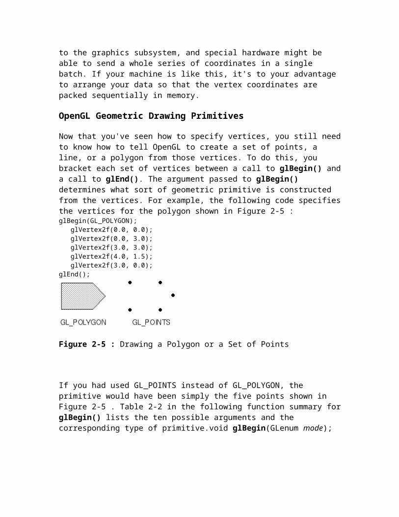
Figure 2-9 : Constructing a Polygon Stipple Pattern    

In addition to defining the current polygon stippling pattern, you must enable stippling:

glEnable(GL_POLYGON_STIPPLE);Use glDisable() with the same argument to disable polygon stippling.

Figure 2-10 shows the results of polygons drawn unstippled and then with two different stippling patterns. The program is shown in Example 2-2 . The reversal of white to black (from Figure 2-9 to Figure 2-10 ) occurs because the program draws in white over a black background, using the pattern in Figure 2-9 as a stencil.

Figure 2-10 : Stippled Polygons    

Example 2-2 : Using Polygon Stipple Patterns: polys.c

#include <GL/gl.h>#include <GL/glu.h>#include "aux.h"

void display(void){    GLubyte fly[] = {        0x00, 0x00, 0x00, 0x00, 0x00, 0x00, 0x00, 0x00,        0x03, 0x80, 0x01, 0xC0, 0x06, 0xC0, 0x03, 0x60,         0x04, 0x60, 0x06, 0x20, 0x04, 0x30, 0x0C, 0x20,         0x04, 0x18, 0x18, 0x20, 0x04, 0x0C, 0x30, 0x20,        0x04, 0x06, 0x60, 0x20, 0x44, 0x03, 0xC0, 0x22,         0x44, 0x01, 0x80, 0x22, 0x44, 0x01, 0x80, 0x22,         0x44, 0x01, 0x80, 0x22, 0x44, 0x01, 0x80, 0x22,        0x44, 0x01, 0x80, 0x22, 0x44, 0x01, 0x80, 0x22,         0x66, 0x01, 0x80, 0x66, 0x33, 0x01, 0x80, 0xCC,         0x19, 0x81, 0x81, 0x98, 0x0C, 0xC1, 0x83, 0x30,        0x07, 0xe1, 0x87, 0xe0, 0x03, 0x3f, 0xfc, 0xc0,         0x03, 0x31, 0x8c, 0xc0, 0x03, 0x33, 0xcc, 0xc0,         0x06, 0x64, 0x26, 0x60, 0x0c, 0xcc, 0x33, 0x30,        0x18, 0xcc, 0x33, 0x18, 0x10, 0xc4, 0x23, 0x08,         0x10, 0x63, 0xC6, 0x08, 0x10, 0x30, 0x0c, 0x08,         0x10, 0x18, 0x18, 0x08, 0x10, 0x00, 0x00, 0x08};

    GLubyte halftone[] = {        0xAA, 0xAA, 0xAA, 0xAA, 0x55, 0x55, 0x55, 0x55,         0xAA, 0xAA, 0xAA, 0xAA, 0x55, 0x55, 0x55, 0x55,         0xAA, 0xAA, 0xAA, 0xAA, 0x55, 0x55, 0x55, 0x55,        0xAA, 0xAA, 0xAA, 0xAA, 0x55, 0x55, 0x55, 0x55,         0xAA, 0xAA, 0xAA, 0xAA, 0x55, 0x55, 0x55, 0x55,         0xAA, 0xAA, 0xAA, 0xAA, 0x55, 0x55, 0x55, 0x55,        0xAA, 0xAA, 0xAA, 0xAA, 0x55, 0x55, 0x55, 0x55,         0xAA, 0xAA, 0xAA, 0xAA, 0x55, 0x55, 0x55, 0x55,         0xAA, 0xAA, 0xAA, 0xAA, 0x55, 0x55, 0x55, 0x55,        0xAA, 0xAA, 0xAA, 0xAA, 0x55, 0x55, 0x55, 0x55,         0xAA, 0xAA, 0xAA, 0xAA, 0x55, 0x55, 0x55, 0x55,         0xAA, 0xAA, 0xAA, 0xAA, 0x55, 0x55, 0x55, 0x55,        0xAA, 0xAA, 0xAA, 0xAA, 0x55, 0x55, 0x55, 0x55,         0xAA, 0xAA, 0xAA, 0xAA, 0x55, 0x55, 0x55, 0x55,         0xAA, 0xAA, 0xAA, 0xAA, 0x55, 0x55, 0x55, 0x55,        0xAA, 0xAA, 0xAA, 0xAA, 0x55, 0x55, 0x55, 0x55};

    glClear (GL_COLOR_BUFFER_BIT);

   glColor3f (1.0, 1.0, 1.0);

    glRectf (25.0, 25.0, 125.0, 125.0);    glEnable (GL_POLYGON_STIPPLE);    glPolygonStipple (fly);    glRectf (125.0, 25.0, 225.0, 125.0);    glPolygonStipple (halftone);    glRectf (225.0, 25.0, 325.0, 125.0);    glDisable (GL_POLYGON_STIPPLE);

    glFlush ();}

void myinit (void) {    glClearColor (0.0, 0.0, 0.0, 0.0);    glShadeModel (GL_FLAT);    }

int main(int argc, char** argv){    auxInitDisplayMode (AUX_SINGLE | AUX_RGBA);    auxInitPosition (0, 0, 350, 150);    auxInitWindow (argv[0]);    myinit ();    auxMainLoop(display);}As mentioned in "Display-List Design Philosophy," you might want to use display lists to store polygon stipple patterns to maximize efficiency.

Marking Polygon Boundary Edges

Advanced

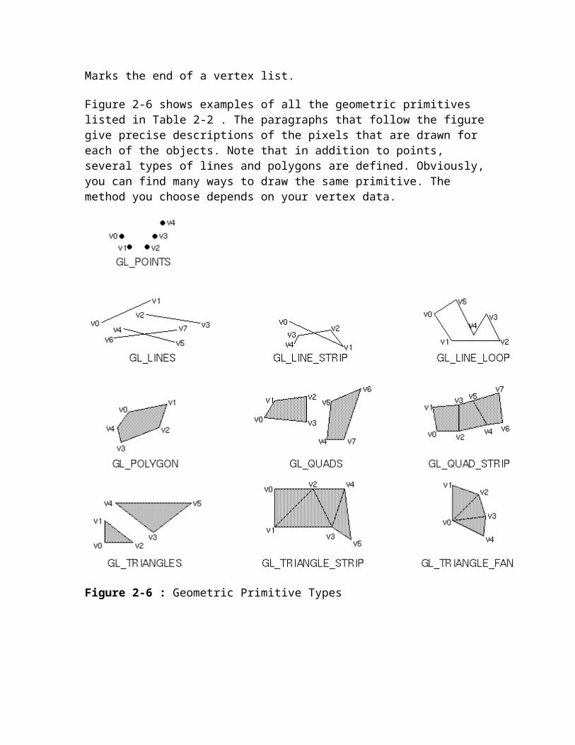
OpenGL can render only convex polygons, but many nonconvex polygons arise in practice. To draw these nonconvex polygons, you typically subdivide them into convex polygons - usually triangles, as shown in Figure 2-11 - and then draw the triangles. Unfortunately, if you decompose a general polygon into triangles and draw the triangles, you can't really use glPolygonMode() to draw the polygon's outline, since you get all the triangle outlines inside it. To solve this problem, you can tell OpenGL whether a particular vertex precedes a boundary edge; OpenGL keeps track of this information by passing along with each vertex a bit indicating whether that vertex is followed by a boundary edge. Then, when a polygon is drawn in GL_LINE mode, the nonboundary edges aren't drawn. In Figure 2-11 , the dashed lines represent added edges.

Figure 2-11 : Subdividing a Nonconvex Polygon    

By default, all vertices are marked as preceding a boundary edge, but you can manually control the setting of the edge flag with the command glEdgeFlag*(). This command is used between glBegin() and glEnd() pairs, and it affects all the vertices specified after it until the next glEdgeFlag() call is made. It applies only to vertices specified for polygons, triangles, and quads, not to those specified for strips of triangles or quads. void glEdgeFlag(GLboolean flag); void glEdgeFlagv(const GLboolean *flag);

Indicates whether a vertex should be considered as initializing a boundary edge of a polygon. If flag is GL_TRUE, the edge flag is set to TRUE (the default), and any vertices created are considered to precede boundary edges until this function is called again with flag being 0.

As an example, Example 2-3 draws the outline shown in Figure 2-12 .

Figure 2-12 : An Outlined Polygon Drawn Using Edge Flags    

Example 2-3 : Marking Polygon Boundary Edges

glPolygonMode(GL_FRONT_AND_BACK, GL_LINE);glBegin(GL_POLYGON);    glEdgeFlag(GL_TRUE);    glVertex3fv(V0);    glEdgeFlag(GL_FALSE);    glVertex3fv(V1);    glEdgeFlag(GL_TRUE);    glVertex3fv(V2);glEnd();

Normal VectorsA normal vector (or normal, for short) is a vector that points in a direction that's perpendicular to a surface. For a flat surface, one perpendicular direction suffices for every point on the surface, but for a general curved surface, the normal direction might be different at each point. With OpenGL, you can specify a normal for each vertex. Vertices might share the same normal, but you can't assign normals anywhere other than at the vertices.

An object's normal vectors define the orientation of its surface in space - in particular, its orientation relative to light sources. These vectors are used by OpenGL to determine how much light the object receives at its vertices. Lighting - a large topic by itself - is the subject of Chapter 6 , and you might want to review the following information after

you've read that chapter. Normal vectors are discussed briefly here because you generally define normal vectors for an object at the same time you define the object's geometry.

You use glNormal*() to set the current normal to the value of the argument passed in. Subsequent calls to glVertex*() cause the specified vertices to be assigned the current normal. Often, each vertex has a different normal, which necessitates a series of alternating calls like this:

glBegin (GL_POLYGON);   glNormal3fv(n0);   glVertex3fv(v0);   glNormal3fv(n1);   glVertex3fv(v1);   glNormal3fv(n2);   glVertex3fv(v2);   glNormal3fv(n3);   glVertex3fv(v3);glEnd();void glNormal3{bsidf}(TYPEnx, TYPEny, TYPEnz); void glNormal3{bsidf}v(const TYPE *v);

Sets the current normal vector as specified by the arguments. The nonvector version (without the v) takes three arguments, which specify an (nx, ny, nz) vector that's taken to be the normal. Alternatively, you can use the vector version of this function (with the v) and supply a single array of three elements to specify the desired normal. The b, s, and i versions scale their parameter values linearly to the range [-1.0,1.0].

There's no magic to finding the normals for an object - most likely, you have to perform some calculations that might include taking derivatives - but there are several techniques and tricks you can use to achieve certain effects. Appendix F explains how to find normal vectors for surfaces. If you already know how to do this, if you can count on always being supplied with normal vectors, or if you don't want to use OpenGL's lighting facility, you don't need to read this appendix.

Note that at a given point on a surface, two vectors are perpendicular to the surface, and they point in opposite directions. By convention, the normal is the one that points to the outside of the surface being modeled. (If you get inside and outside reversed in your model, just change every normal vector from (x, y, z) to (-x, -y, -z)).

Also, keep in mind that since normal vectors indicate direction only, their length is mostly irrelevant. You can specify normals of any length, but eventually they have to be converted to having a length of 1 before lighting calculations are performed. (A vector that has a length of 1 is said to be of unit length, or normalized.) In general, then, you should supply normalized normal vectors. These vectors remain normalized as long as your model transformations include only rotations and translations. (Transformations are discussed in detail in Chapter 3 .) If you perform irregular transformations (such as scaling or multiplying by a shear matrix), or if you specify nonunit-length normals, then you should have OpenGL automatically normalize your normal vectors after the

transformations. To do this, call glEnable() with GL_NORMALIZE as its argument. By default, automatic normalization is disabled. Note that in some implementations of OpenGL, automatic normalization requires additional calculations that might reduce the performance of your application.

Some Hints for Building Polygonal Models of SurfacesFollowing are some techniques that you might want to use as you build polygonal approximations of surfaces. You might want to review this section after you've read Chapter 6 on lighting and Chapter 4 on display lists. The lighting conditions affect how models look once they're drawn, and some of the following techniques are much more efficient when used in conjunction with display lists. As you read these techniques, keep in mind that when lighting calculations are enabled, normal vectors must be specified to get proper results.

Constructing polygonal approximations to surfaces is an art, and there is no substitute for experience. This section, however, lists a few pointers that might make it a bit easier to get started.

Keep polygon orientations consistent. Make sure that when viewed from the outside, all the polygons on the surface are oriented in the same direction (all clockwise or all counterclockwise). Try to get this right the first time, since it's excruciatingly painful to fix the problem later.  

When you subdivide a surface, watch out for any nontriangular polygons. The three vertices of a triangle are guaranteed to lie on a plane; any polygon with four or more vertices might not. Nonplanar polygons can be viewed from some orientation such that the edges cross each other, and OpenGL might not render such polygons correctly.  

There's always a trade-off between the display speed and the quality of the image. If you subdivide a surface into a small number of polygons, it renders quickly but might have a jagged appearance; if you subdivide it into millions of tiny polygons, it probably looks good but might take a long time to render. Ideally, you can provide a parameter to the subdivision routines that indicates how fine a subdivision you want, and if the object is farther from the eye, you can use a coarser subdivision. Also, when you subdivide, use relatively large polygons where the surface is relatively flat, and small polygons in regions of high curvature.  

For high-quality images, it's a good idea to subdivide more on the silhouette edges than in the interior. If the surface is to be rotated relative to the eye, this is tougher to do, since the silhouette edges keep moving. Silhouette edges occur where the normal vectors are perpendicular to the vector from the surface to the viewpoint - that is, when their vector dot product is zero. Your subdivision algorithm might choose to subdivide more if this dot product is near zero.  

Try to avoid T-intersections in your models (see Figure 2-13 ). As shown, there's no guarantee that the line segments AB and BC lie on exactly the same pixels as the segment AC. Sometimes they do, and sometimes they don't, depending on the transformations and orientation. This can cause cracks to appear intermittently in the surface.

Figure 2-13 : Modifying an Undesirable T-intersection    

If you're constructing a closed surface, make sure to use exactly the same numbers for coordinates at the beginning and end of a closed loop, or you can get gaps and cracks due to numerical round-off. Here's a two-dimensional example of bad code: /* don't use this code */

    #define PI 3.14159265     #define EDGES 30 

    /* draw a circle */     for (i = 0; i < EDGES; i++) {       glBegin(GL_LINE_STRIP);         glVertex2f(cos((2*PI*i)/EDGES), sin((2*PI*i)/EDGES);         glVertex2f(cos((2*PI*(i+1))/EDGES),                       sin((2*PI*(i+1))/EDGES);       glEnd();     }The edges meet exactly only if your machine manages to calculate the sine and cosine of 0 and of (2*PI*EDGES/EDGES) and gets exactly the same values. If you trust the floating-point unit on your machine to do this right, the authors have a bridge they'd like to sell you.... To correct the code, make sure that when i == EDGES-1, you use 0 for the sine and cosine, not 2*PI*EDGES/EDGES.  

Finally, note that unless tessellation is very fine, any change is likely to be visible. In some animations, these changes are more visually disturbing than the artifacts of undertessellation.

An Example: Building an Icosahedron

To illustrate some of the considerations that arise in approximating a surface, let's look at some example code sequences. This code concerns the vertices of a regular icosahedron (which is a Platonic solid composed of twenty faces that span twelve vertices, each face of which is an equilateral triangle). An icosahedron can be considered a rough approximation for a sphere. Example 2-4 defines the vertices and triangles making up an icosahedron and then draws the icosahedron.

Example 2-4 : Drawing an Icosahedron

#define X .525731112119133606 #define Z .850650808352039932

static GLfloat vdata[12][3] = {       {-X, 0.0, Z}, {X, 0.0, Z}, {-X, 0.0, -Z}, {X, 0.0, -Z},       {0.0, Z, X}, {0.0, Z, -X}, {0.0, -Z, X}, {0.0, -Z, -X},       {Z, X, 0.0}, {-Z, X, 0.0}, {Z, -X, 0.0}, {-Z, -X, 0.0} };

static GLint tindices[20][3] = {    {0,4,1}, {0,9,4}, {9,5,4}, {4,5,8}, {4,8,1},       {8,10,1}, {8,3,10}, {5,3,8}, {5,2,3}, {2,7,3},       {7,10,3}, {7,6,10}, {7,11,6}, {11,0,6}, {0,1,6},    {6,1,10}, {9,0,11}, {9,11,2}, {9,2,5}, {7,2,11} };

for (i = 0; i < 20; i++) {       /* color information here */    glBegin(GL_TRIANGLE);          glVertex3fv(&vdata[tindices[i][0]][0]);       glVertex3fv(&vdata[tindices[i][1]][0]);       glVertex3fv(&vdata[tindices[i][2]][0]);       glEnd(); }The strange numbers X and Z are chosen so that the distance from the origin to any of the vertices of the icosahedron is 1.0. The coordinates of the twelve vertices are given in the array vdata[][], where the zeroth vertex is {-X, 0.0, Z}, the first is {X, 0.0, Z}, and so on. The array tindices[][] tells how to link the vertices to make triangles. For example, the first triangle is made from the zeroth, fourth, and first vertex. If you take the vertices for triangles in the order given, all the triangles have the same orientation.

The line that mentions color information should be replaced by a command that sets the color of the ith face. If no code appears here, all faces are drawn in the same color, and it'll be impossible to discern the three-dimensional quality of the object. An alternative to explicitly specifying colors is to define surface normals and use lighting, as described in the next section.

In all the examples described in this section, unless the surface is to be drawn only once, you should probably save the calculated vertex and normal coordinates so that the calculations don't need to be repeated each time that the surface is drawn. This can be done using your own data structures or by constructing display lists (see Chapter 4 .)

Defining the Icosahedron's Normals

If the icosahedron is to be lit, you need to supply the vector normal to the surface. With the flat surfaces of an icosahedron, all three vertices defining a surface have the same normal vector. Thus, the normal needs to be specified only once for each set of three vertices. The code in Example 2-5 can replace the "color information here" line in Example 2-4 for drawing the icosahedron.

Example 2-5 : Supplying Normals for an Icosahedron

GLfloat d1[3], d2[3], norm[3];    for (j = 0; j < 3; j++) {       d1[j] = vdata[tindices[i][0]][j] - vdata[tindices[i][1]][j];       d2[j] = vdata[tindices[i][1]][j] - vdata[tindices[i][2]][j];    }normcrossprod(d1, d2, norm); glNormal3fv(norm);The function normcrossprod() produces the normalized cross product of two vectors, as shown in Example 2-6 .

Example 2-6 : Calculating the Normalized Cross Product of Two Vectors

void normalize(float v[3]) {       GLfloat d = sqrt(v[1]*v[1]+v[2]*v[2]+v[3]*v[3]);    if (d == 0.0) {      error("zero length vector");          return;   }   v[1] /= d; v[2] /= d; v[3] /= d; }

void normcrossprod(float v1[3], float v2[3], float out[3]) {    GLint i, j;    GLfloat length;

   out[0] = v1[1]*v2[2] - v1[2]*v2[1];    out[1] = v1[2]*v2[0] - v1[0]*v2[2];    out[2] = v1[0]*v2[1] - v1[1]*v2[0];    normalize(out); }If you're using an icosahedron as an approximation for a shaded sphere, you'll want to use normal vectors that are perpendicular to the true surface of the sphere, rather than being perpendicular to the faces. For a sphere, the normal vectors are simple; each points in the same direction as the vector from the origin to the corresponding vertex. Since the icosahedron vertex data is for an icosahedron of radius 1, the normal and vertex data is

identical. Here is the code that would draw an icosahedral approximation of a smoothly shaded sphere (assuming that lighting is enabled, as described in Chapter 6 ): for (i = 0; i < 20; i++) {       glBegin(GL_POLYGON);       glNormal3fv(&vdata[tindices[i][0]][0]);       glVertex3fv(&vdata[tindices[i][0]][0]);       glNormal3fv(&vdata[tindices[i][1]][0]);       glVertex3fv(&vdata[tindices[i][1]][0]);       glNormal3fv(&vdata[tindices[i][2]][0]);       glVertex3fv(&vdata[tindices[i][2]][0]);       glEnd(); }

Improving the Model

A twenty-sided approximation to a sphere doesn't look good unless the image of the sphere on the screen is quite small, but there's an easy way to increase the accuracy of the approximation. Imagine the icosahedron inscribed in a sphere, and subdivide the triangles as shown in Figure 2-14 . The newly introduced vertices lie slightly inside the sphere, so push them to the surface by normalizing them (dividing them by a factor to make them have length 1). This subdivision process can be repeated for arbitrary accuracy. The three objects shown in Figure 2-14 use twenty, eighty, and three hundred and twenty approximating triangles, respectively.

Figure 2-14 : Subdividing to Improve a Polygonal Approximation to a Surface    

Example 2-7 performs a single subdivision, creating an eighty-sided spherical approximation.

Example 2-7 : Single Subdivision

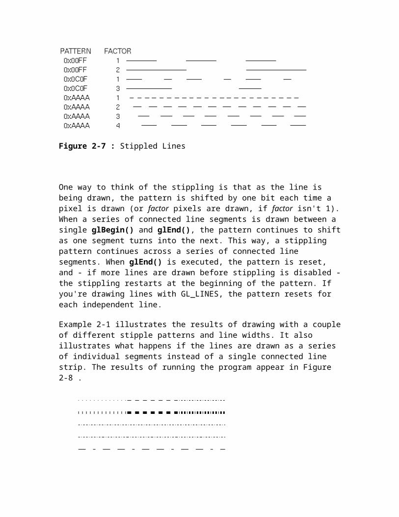
void drawtriangle(float *v1, float *v2, float *v3) {    glBegin(GL_POLYGON);       glNormal3fv(v1); vlVertex3fv(v1);          glNormal3fv(v2); vlVertex3fv(v2);          glNormal3fv(v3); vlVertex3fv(v3);       glEnd(); }

void subdivide(float *v1, float *v2, float *v3) {    GLfloat v12[3], v23[3], v31[3];       GLint i;

   for (i = 0; i < 3; i++) {       v12[i] = v1[i]+v2[i];       v23[i] = v2[i]+v3[i];           v31[i] = v3[i]+v1[i];       }    normalize(v12);       normalize(v23);    normalize(v31);    drawtriangle(v1, v12, v31);       drawtriangle(v2, v23, v12);       drawtriangle(v3, v31, v23);       drawtriangle(v12, v23, v31); }

for (i = 0; i < 20; i++) {    subdivide(&vdata[tindices[i][0]][0],                   &vdata[tindices[i][1]][0],                    &vdata[tindices[i][2]][0]); }Example 2-8 is a slight modification of Example 2-7 that recursively subdivides the triangles to the proper depth. If the depth value is 0, no subdivisions are performed, and the triangle is drawn as is. If the depth is 1, a single subdivison is performed, and so on.

Example 2-8 : Recursive Subdivision

void subdivide(float *v1, float *v2, float *v3, long depth){   GLfloat v12[3], v23[3], v31[3];   GLint i;

   if (depth == 0) {      drawtriangle(v1, v2, v3);       return;   }   for (i = 0; i < 3; i++) {       v12[i] = v1[i]+v2[i];      v23[i] = v2[i]+v3[i];      v31[i] = v3[i]+v1[i];   }   normalize(v12);   normalize(v23);

   normalize(v31);   subdivide(v1, v12, v31, depth-1);   subdivide(v2, v23, v12, depth-1);   subdivide(v3, v31, v23, depth-1);   subdivide(v12, v23, v31, depth-1);}

Generalized Subdivision

A recursive subdivision technique such as the one described in Example 2-8 can be used for other types of surfaces. Typically, the recursion ends either if a certain depth is reached, or if some condition on the curvature is satisfied (highly curved parts of surfaces look better with more subdivision).

To look at a more general solution to the problem of subdivision, consider an arbitrary surface parameterized by two variables u[0] and u[1]. Suppose that two routines are provided:

void surf(GLfloat u[2], GLfloat vertex[3], GLfloat normal[3]); float curv(GLfloat u[2]);If surf() is passed u[], the corresponding three-dimensional vertex and normal vectors (of length 1) are returned. If u[] is passed to curv(), the curvature of the surface at that point is calculated and returned. (See an introductory textbook on differential geometry for more information about measuring surface curvature.)

Example 2-9 shows the recursive routine that subdivides a triangle either until the maximum depth is reached or until the maximum curvature at the three vertices is less than some cutoff.

Example 2-9 : Generalized Subdivision

void subdivide(float u1[2], float u2[2], float u3[2],                float cutoff, long depth){   GLfloat v1[3], v2[3], v3[3], n1[3], n2[3], n3[3];   GLfloat u12[2], u23[2], u32[2];   GLint i;

   if (depth == maxdepth || (curv(u1) < cutoff &&       curv(u2) < cutoff && curv(u3) < cutoff)) {      surf(u1, v1, n1); surf(u2, v2, n2); surf(u3, v3, n3);       glBegin(GL_POLYGON);          glNormal3fv(n1); glVertex3fv(v1);          glNormal3fv(n2); glVertex3fv(v2);          glNormal3fv(n3); glVertex3fv(v3);      glEnd();      return;   }   for (i = 0; i < 2; i++) {       u12[i] = (u1[i] + u2[i])/2.0;       u23[i] = (u2[i] + u3[i])/2.0;       u31[i] = (u3[i] + u1[i])/2.0;

   }   subdivide(u1, u12, u31, cutoff, depth+1);   subdivide(u2, u23, u12, cutoff, depth+1);   subdivide(u3, u31, u23, cutoff, depth+1);   subdivide(u12, u23, u31, cutoff, depth+1);}

[Previous chapter] [Next chapter]

See the About page for copyright, authoring and distribution information.

Chapter 3ViewingChapter Objectives

After reading this chapter, you'll be able to do the following:

View a geometric model in any orientation by transforming it in three-dimensional space  

Control the location in three-dimensional space from which the model is viewed  

Clip undesired portions of the model out of the scene that's to be viewed  

Manipulate the appropriate matrix stacks that control model transformation for viewing and project the model onto the screen  

Combine multiple transformations to mimic sophisticated systems in motion, such as a solar system or an articulated robot arm

Chapter 2 explained how to instruct OpenGL to draw the geometric models you want displayed in your scene. Now you must decide how you want to position the models in the scene, and you must choose a vantage point from which to view the scene. You can use the default positioning and vantage point, but most likely you want to specify them.

Look at the image on the cover of this book. The program that produced that image contained a single geometric description of a building block. Each block was carefully positioned in the scene: Some blocks were scattered on the floor, some were stacked on top of each other on the table, and some were assembled to make the globe. Also, a particular viewpoint had to be chosen. Obviously, we wanted to look at the corner of the room containing the globe. But how far away from the scene - and where exactly - should the viewer be? We wanted to make sure that the final image of the scene contained a good view out the window, that a portion of the floor was visible, and that all the objects in the scene were not only visible but presented in an interesting arrangement. This chapter explains how to use OpenGL to accomplish these tasks: how to position and orient models in three-dimensional space and how to establish the location - also in three-

dimensional space - of the viewpoint. All of these factors help determine exactly what image appears on the sceen.

You want to remember that the point of computer graphics is to create a two-dimensional image of three-dimensional objects (it has to be two-dimensional because it's drawn on the screen), but you need to think in three-dimensional coordinates while making many of the decisions that determine what gets drawn on the screen. A common mistake people make when creating three-dimensional graphics is to start thinking too soon that the final image appears on a flat, two-dimensional screen. Avoid thinking about which pixels need to be drawn, and instead try to visualize three-dimensional space. Create your models in some three-dimensional universe that lies deep inside your computer, and let the computer do its job of calculating which pixels to color.

A series of three computer operations convert an object's three-dimensional coordinates to pixel positions on the screen:

Transformations, which are represented by matrix multiplication, include modeling, viewing, and projection operations. Such operations include rotation, translation, scaling, reflecting, orthographic projection, and perspective projection. Generally, you use a combination of several transformations to draw a scene.  

Since the scene is rendered on a rectangular window, objects (or parts of objects) that lie outside the window must be clipped. In three-dimensional computer graphics, clipping occurs by throwing out objects on one side of a clipping plane.  

Finally, a correspondence must be established between the transformed coordinates and screen pixels. This is known as a viewport transformation.

This chapter describes all of these operations, and how to control them, in the following major sections:

"Overview: The Camera Analogy" gives an overview of the transformation process by describing the analogy of taking a photograph with a camera, presents a simple example program that transforms an object, and briefly describes the basic OpenGL transformation commands.  

"Viewing and Modeling Transformations" explains in detail how to specify and to imagine the effect of viewing and modeling transformations. These transformations orient the model and the camera relative to each other to obtain the desired final image.  

"Projection Transformations" describes how to specify the shape and orientation of the viewing volume. The viewing volume determines how a scene is projected onto the screen (with a perspective or orthographic projection) and which objects or parts of objects are clipped out of the scene.  

"Viewport Transformation" explains how to control the conversion of three-dimensional model coordinates to screen coordinates.  

"Troubleshooting Transformations" presents some tips for discovering why you might not be getting the desired effect from your modeling, viewing, projection, and viewport transformations.  

"Manipulating the Matrix Stacks" discusses how to save and restore certain transformations. This is particularly useful when you're drawing complicated objects that are built up from simpler ones.  

"Additional Clipping Planes" describes how to specify additional clipping planes beyond those defined by the viewing volume.  

"Examples of Composing Several Transformations" walks you through a couple of more complicated uses for transformations.

Overview: The Camera AnalogyThe transformation process to produce the desired scene for viewing is analogous to taking a photograph with a camera. As shown in Figure 3-1 , the steps with a camera (or a computer) might be the following:

Setting up your tripod and pointing the camera at the scene (viewing transformation).  

Arranging the scene to be photographed into the desired composition (modeling transformation).  

Choosing a camera lens or adjusting the zoom (projection transformation).  

Determining how large you want the final photograph to be - for example, you might want it enlarged (viewport transformation).

After these steps are performed, the picture can be snapped, or the scene can be drawn.

Figure 3-1 : The Camera Analogy    

Note that these steps correspond to the order in which you specify the desired transformations in your program, not necessarily the order in which the relevant mathematical operations are performed on an object's vertices. The viewing transformations must precede the modeling transformations in your code, but you can specify the projection and viewport transformations at any point before drawing occurs. Figure 3-2 shows the order in which these operations occur on your computer.

Figure 3-2 : Stages of Vertex Transformation    

To specify viewing, modeling, and projection transformations, you construct a 4 4נ matrix M, which is then multiplied by the coordinates of each vertex v in the scene to accomplish the transformation

v'=Mv

(Remember that vertices always have four coordinates (x ,y, z, w), though in most cases w is 1 and for two-dimensional data z is 0.) Note that viewing and modeling transformations are automatically applied to surface normal vectors, in addition to vertices. (Normal vectors are used only in eye coordinates.) This ensures that the normal vector's relationship to the vertex data is properly preserved.

The viewing and modeling transformations you specify are combined to form the modelview matrix, which is applied to the incoming object coordinates to yield eye coordinates. Next, if you've specified arbitrary clipping planes to remove certain objects from the scene or to provide cutaway views of objects, these clipping planes are applied.

After that, OpenGL applies the projection matrix to yield clip coordinates. This transformation defines a viewing volume; objects outside this volume are clipped so that they're not drawn in the final scene. After this point, the perspective division is performed by dividing coordinate values by w, to produce normalized device coordinates. (See Appendix G for more information about the meaning of the w coordinate and how it affects matrix transformations.) Finally, the transformed coordinates are converted to window coordinates by applying the viewport transformation. You can manipulate the dimensions of the viewport to cause the final image to be enlarged, shrunk, or stretched.

You might correctly suppose that the x and y coordinates are sufficient to determine which pixels need to be drawn on the screen. However, all the transformations are performed on the z coordinates as well. This way, at the end of this transformation process, the z values correctly reflect the depth of a given vertex (measured in distance away from the screen). One use for this depth value is to eliminate unnecessary drawing. For example, suppose two vertices have the same x and y values but different z values. OpenGL can use this information to determine which surfaces are obscured by other surfaces and can then avoid drawing the hidden surfaces. (See Chapter 10 for more information about this technique, which is called hidden-surface removal.)

As you've probably guessed by now, you need to know a few things about matrix mathematics to get the most out of this chapter. If you want to brush up on your knowledge in this area, you might consult a textbook on linear algebra.

A Simple Example: Drawing a Cube

Example 3-1 draws a cube that's scaled by a modeling transformation (see Figure 3-3 ). The viewing transformation used is a simple translation down the z-axis. A projection transformation and a viewport transformation are also specified. The rest of this section walks you through Example 3-1 and briefly explains the transformation commands it uses. The succeeding sections contain the complete, detailed discussion of all OpenGL's transformation commands.

Figure 3-3 : A Transformed Cube    

Example 3-1 : A Transformed Cube: cube.c

#include <GL/gl.h>#include <GL/glu.h>

#include "aux.h"

void display (void){    glClear(GL_COLOR_BUFFER_BIT);    glColor3f (1.0, 1.0, 1.0);    glLoadIdentity ();             /* clear the matrix */    glTranslatef (0.0, 0.0, -5.0); /* viewing transformation */    glScalef (1.0, 2.0, 1.0);      /* modeling transformation */    auxWireCube(1.0);    /*  draw the cube */    glFlush();}

void myinit (void) {    glShadeModel (GL_FLAT);}

void myReshape(GLsizei w, GLsizei h){    glMatrixMode (GL_PROJECTION);    /* prepare for and then */     glLoadIdentity ();               /* define the projection */    glFrustum (-1.0, 1.0, -1.0, 1.0, /* transformation */                   1.5, 20.0);     glMatrixMode (GL_MODELVIEW);  /* back to modelview matrix */    glViewport (0, 0, w, h);      /* define the viewport */}

int main(int argc, char** argv){    auxInitDisplayMode (AUX_SINGLE | AUX_RGBA);    auxInitPosition (0, 0, 500, 500);    auxInitWindow (argv[0]);    myinit ();    auxReshapeFunc (myReshape);    auxMainLoop(display);}

The Viewing Transformation

Recall that the viewing transformation is analogous to positioning and aiming a camera. In this code example, before the viewing transformation can be specified, the current matrix is set to the identity matrix with glLoadIdentity(). This step is necessary since most of the transformation commands multiply the current matrix by the specified matrix and then set the result to be the current matrix. If you don't clear the current matrix by loading it with the identity matrix, you continue to combine previous transformation matrices with the new one you supply. In some cases, you do want to perform such combinations, but you also need to clear the matrix sometimes.

Once the matrix is initialized, the viewing transformation is specified with glTranslatef(). The arguments for this command indicate how the camera should be translated (moved) in the x, y, and z directions. The arguments used here move the

camera 5 units in the negative z direction. By default, the camera as well as any objects in the scene are originally situated at the origin; also, the camera initially points down the negative z-axis. Thus, the particular viewing transformation used here has the effect of pulling the camera away from where the cube is, but it leaves the camera pointing at the object. If the camera needed to be pointed in another direction, you could have used the glRotatef() command to change its orientation. Viewing transformations are discussed in detail in "Viewing and Modeling Transformations."

The Modeling Transformation

You use the modeling transformation to position and orient the model. For example, you can rotate, translate, or scale the model - or perform some combination of these operations. Rotating and translating are performed using the commands already mentioned - glRotatef() and glTranslatef(). In this example, however, the modeling transformation is invoked with glScalef(). The arguments for this command specify how scaling should occur along the three axes. If all the arguments are 1.0, this command has no effect; in Example 3-1 , the cube is drawn twice as large in the y direction. Thus, if one corner of the cube had originally been at (3.0, 3.0, 3.0), that corner would wind up being drawn at (3.0, 6.0, 3.0). The effect of this modeling transformation is to transform the cube so that it isn't a cube but a rectangular box.

Note that instead of pulling the camera back away from the cube (with a viewing transformation) so that it could be viewed, you could have moved the cube away from the camera (with a modeling transformation). This duality in the nature of viewing and modeling transformations is why you need to think about the effect of both types of transformations simultaneously. It doesn't make sense to try to separate the effects, but sometimes it's easier to think about them one way rather than the other. This is also why modeling and viewing transformations are combined into the modelview matrix before the transformations are applied. "Viewing and Modeling Transformations," explains in more detail how to think about modeling and viewing transformations and how to specify them so that you get the result you want.

Also note that the modeling and viewing transformations are included in the display() routine, along with the call that's used to draw the cube, auxWireCube(). This way, display() can be used repeatedly to draw the contents of the window if, for example, the window is moved or uncovered, and you've ensured that each time, the cube is drawn in the desired way, with the appropriate transformations. The potential repeated use of display() underscores the need to load the identity matrix before performing the viewing and modeling transformations, especially when other transformations might be performed between calls to display().

The Projection Transformation

Specifying the projection transformation is like choosing a lens for a camera. You can think of this transformation as determining what the field of view or viewing volume is and therefore what objects are inside it and to some extent how they look. This is

equivalent to choosing among wide-angle, normal, and telephoto lenses, for example. With a wide-angle lens, you can include a wider scene in the final photograph than with a telephoto lens, but a telephoto lens allows you to photograph objects as though they're closer to you than they actually are. In computer graphics, you don't have to pay $10,000 for a 2000-millimeter telephoto lens; once you've bought your graphics workstation, all you need to do is use a smaller number for your field of view.

In addition to the field-of-view considerations, the projection transformation determines how objects are projected onto the screen, as its name suggests. Two basic types of projections are provided for you by OpenGL, along with several corresponding commands for describing the relevant parameters in different ways. One type is the perspective projection, which matches how you see things in daily life. Perspective makes objects that are farther away appear smaller; for example, it makes railroad tracks appear to converge in the distance. If you're trying to make realistic pictures, you'll want to choose perspective projection, which is specified with the glFrustum() command in this code example.

The other type of projection is orthographic, which maps objects directly onto the screen without affecting their relative size. Orthographic projection is used in architectural and computer-aided design applications where the final image needs to reflect the measurements of objects rather than how they might look. Architects create perspective drawings to show how particular buildings or interior spaces look when viewed from various vantage points; the need for orthographic projection arises when blueprint plans or elevations are generated, which are used in the construction of buildings. "Projection Transformations," discusses the ways to specify both kinds of projection transformations in more detail.

Before glFrustum() can be called to set the projection transformation, some preparation needs to happen. As shown in the myReshape() routine in Example 3-1 , the command called glMatrixMode() is used first, with the argument GL_PROJECTION. This indicates that the current matrix specifies the projection transformation; the following transformation calls then affect the projection matrix. As you can see, a few lines later glMatrixMode() is called again, this time with GL_MODELVIEW as the argument. This indicates that succeeding transformations now affect the modelview matrix instead of the projection matrix. See "Manipulating the Matrix Stacks," for more information about how to control the projection and modelview matrices.

Note that glLoadIdentity() is used to initialize the current projection matrix so that only the specified projection transformation has an effect. Now glFrustum() can be called, with arguments that define the parameters of the projection transformation. In this example, both the projection transformation and the viewport transformation are contained in the myReshape() routine, which is called when the window is first created and whenever the window is moved or reshaped. This makes sense, since both projecting and applying the viewport relate directly to the screen, and specifically to the size of the window on the screen.

The Viewport Transformation

Together, the projection transformation and the viewport transformation determine how a scene gets mapped onto the computer screen. The projection transformation specifies the mechanics of how the mapping should occur, and the viewport indicates the shape of the available screen area into which the scene is mapped. Since the viewport specifies the region the image occupies on the computer screen, you can think of the viewport transformation as defining the size and location of the final processed photograph - whether it should be enlarged or shrunk, for example.

The arguments to glViewport() describe the origin of the available screen space within the window - (0, 0) in this example - and the width and height of the available screen area, all measured in pixels on the screen. This is why this command needs to be called within myReshape() - if the window changes size, the viewport needs to change accordingly. Note that the width and height are specified using the actual width and height of the window; often, you want to specify the viewport this way rather than giving an absolute size. See "Viewport Transformation," for more information about how to define the viewport.

Drawing the Scene

Once all the necessary transformations have been specified, you can draw the scene (that is, take the photograph). As the scene is drawn, OpenGL transforms each vertex of every object in the scene by the modeling and viewing transformations. Each vertex is then transformed as specified by the projection transformation and clipped if it lies outside the viewing volume described by the projection transformation. Finally, the remaining transformed vertices are divided by w and mapped onto the viewport.

General-Purpose Transformation Commands

This section discusses some OpenGL commands that you might find useful as you specify desired transformations. You've already seen a couple of these commands, glMatrixMode() and glLoadIdentity(). The other two commands described here - glLoadMatrix*() and glMultMatrix*() - allow you to specify any transformation matrix directly and then to multiply the current matrix by that specified matrix. More specific transformation commands - such as glTranslate*() and glScale*() - are described in later sections.

As described in the preceding section, you need to state whether you want to modify the modelview or projection matrix before supplying a transformation command. You do this with glMatrixMode(). When you use nested sets of OpenGL commands that might be called repeatedly, remember to reset the matrix mode correctly. (The glMatrixMode() command can also be used to indicate the texture matrix; texturing is discussed in detail in Chapter 9 .)void glMatrixMode(GLenum mode);

Specifies whether the modelview, projection, or texture matrix will be modified, using the argument GL_MODELVIEW, GL_PROJECTION, or GL_TEXTURE for mode. Subsequent transformation commands affect the specified matrix. Note that only one matrix can be modified at a time. By default, the modelview matrix is the one that's modifiable, and all three matrices contain the identity matrix.

You use the glLoadIdentity() command to clear the currently modifiable matrix for future transformation commands, since these commands modify the current matrix. Typically, you always call this command before specifying projection or viewing transformations, but you might also call it before specifying a modeling transformation.void glLoadIdentity(void);

Sets the currently modifiable matrix to the 4 4נ identity matrix.

If you want to explicitly specify a particular matrix to be loaded as the current matrix, use glLoadMatrix*(). Similarly, use glMultMatrix*() to multiply the current matrix by the matrix passed in as an argument. The argument for both these commands is a vector of sixteen values (m1, m2, ... , m16) that specifies a matrix M as follows:

Remember that you might be able to maximize efficiency by using display lists to store frequently used matrices (and their inverses) rather than recomputing them; see "Display-List Design Philosophy." (OpenGL implementations often must compute the inverse of the modelview matrix so that normals and clipping planes can be correctly transformed to eye coordinates.)

If you're programming in C, and you declare a matrix as m[4][4], then the element m[i][j] is in the ith column and jth row of the OpenGL transformation matrix. This is the reverse of the standard C convention in which m[i][j] is in row i and column j. To avoid confusion, you should declare your matrices as m[16]. void glLoadMatrix{fd}(const TYPE *m);

Sets the sixteen values of the current matrix to those specified by m.

void glMultMatrix{fd}(const TYPE *m);

Multiplies the matrix specified by the sixteen values pointed to by m by the current matrix and stores the result as the current matrix.

All matrix multiplication with OpenGL occurs as follows: Suppose the current matrix is C and the matrix specified with glMultMatrix*() or any of the transformation commands is M. After multiplication, the final matrix is always CM. Since matrix multiplication isn't generally commutative, the order makes a difference.

 

Viewing and Modeling TransformationsAs noted in "A Simple Example: Drawing a Cube," viewing and modeling transformations are inextricably related in OpenGL and are in fact combined into a single modelview matrix. One of the toughest problems newcomers to computer graphics face is understanding the effects of combined three-dimensional transformations. As you've already seen, there are alternative ways to think about transformations - do you want to move the camera in one direction, or move the object in the opposite direction? Each way of thinking about transformations has advantages and disadvantages, but in some cases one way more naturally matches the effect of the intended transformation. If you can find a natural approach for your particular application, it's easier to visualize the necessary transformations and then write the corresponding code to specify the matrix manipulations. The first part of this section discusses how to think about transformations; later, specific commands are presented. For now, we use only the matrix-manipulation commands you've already seen. Finally, keep in mind that you must call glMatrixMode() with GL_MODELVIEW as its argument prior to performing modeling or viewing transformations.

Thinking about Transformations

Let's start with a simple case of two transformations: a 45-degree counterclockwise rotation about the origin around the z-axis, and a translation down the x-axis. Suppose that the object you're drawing is small compared to the translation (so that you can see the effect of the translation), and that it's originally located at the origin. If you rotate the object first and then translate it, the rotated object appears on the x-axis. If you translate it down the x-axis first, however, and then rotate about the origin, the object is on the line y=x, as shown in Figure 3-4 . In general, the order of transformations is critical. If you do transformation A and then transformation B, you almost certainly get something different than if you do them in the opposite order.

Figure 3-4 : Rotating First or Translating First    

Now let's talk about the order in which you specify a series of transformations. All viewing and modeling transformations are represented as 4 4נ matrices. Each successive glMultMatrix*() or transformation command multiplies a new 4 4נ matrix M by the current modelview matrix C to yield CM. Finally, vertices v are multiplied by the current modelview matrix. This process means that the last transformation command called in your program is actually the first one applied to the vertices: CMv. Thus, one way of looking at it is to say that you have to specify the matrices in the reverse order. Like many other things, however, once you've gotten used to thinking about this correctly, backward will seem like forward.

Consider the following code sequence, which draws a single point using three transformations:

glMatrixMode(GL_MODELVIEW);glLoadIdentity();glMultMatrixf(N);                     /* apply transformation N */glMultMatrixf(M);                     /* apply transformation M */glMultMatrixf(L);                     /* apply transformation L */glBegin(GL_POINTS);glVertex3f(v);                        /* draw transformed vertex v */glEnd();With this code, the modelview matrix successively contains I, N, NM, and finally NML, where I represents the identity matrix. The transformed vertex is NMLv. Thus, the vertex transformation is N(M(Lv)) - that is, v is multiplied first by L, the resulting Lv is multiplied by M, and the resulting MLv is multiplied by N. Notice that the transformations to vertex v effectively occur in the opposite order than they were specified. (Actually, only a single multiplication of a vertex by the modelview matrix occurs; in this example, the N, M, and L matrices are already multiplied into a single matrix before it's applied to v.)

Thus, if you like to think in terms of a grand, fixed coordinate system - in which matrix multiplications affect the position, orientation, and scaling of your model - you have to think of the multiplications as occurring in the opposite order from how they appear in the code. Using the simple example discussed in Figure 3-4 (a rotation about the origin and a translation along the x-axis), if you want the object to appear on the axis after the operations, the rotation must occur first, followed by the translation. To do this, the code looks something like this (where R is the rotation matrix and T is the translation matrix):

glMatrixMode(GL_MODELVIEW);glLoadIdentity();glMultMatrixf(T);                     /* translation */glMultMatrixf(R);                     /* rotation */draw_the_object();Another way to view matrix multiplications is to forget about a grand, fixed coordinate system in which your model is transformed and instead imagine that a local coordinate system is tied to the object you're drawing. All operations occur relative to this changing coordinate system. With this approach, the matrix multiplications now appear in the natural order in the code. (Regardless of which analogy you're using, the code is the same, but how you think about it differs.) To see this in the translation-rotation example, begin by visualizing the object with a coordinate system tied to it. The translation operation moves the object and its coordinate system down the x-axis. Then, the rotation occurs about the (now-translated) origin, so the object rotates in place in its position on the axis.

This approach is what you should use for applications such as articulated robot arms, where there are joints at the shoulder, elbow, and wrist, and on each of the fingers. To figure out where the tips of the fingers go relative to the body, you'd like to start at the shoulder, go down to the wrist, and so on, applying the appropriate rotations and translations at each joint. Thinking about it in reverse would be far more confusing.

This second approach can be problematic, however, in cases where scaling occurs, and especially so when the scaling is nonuniform (scaling different amounts along the different axes). After uniform scaling, translations move a vertex by a multiple of what they did before, since the coordinate system is stretched. Nonuniform scaling mixed with rotations may make the axes of the local coordinate system nonperpendicular.

As mentioned earlier, you normally issue viewing transformation commands in your program before any modeling transformations. This way, a vertex in a model is first transformed into the desired orientation and then transformed by the viewing operation. Since the matrix multiplications must be specified in reverse order, the viewing commands need to come first. Note, however, that you don't need to specify either viewing or modeling transformations if you're satisfied with the default conditions. If there's no viewing transformation, the "camera" is left in the default position at the origin, pointed toward the negative z-axis; if there's no modeling transformation, the model isn't moved, and it retains its specified position, orientation, and size.

Since the commands for performing modeling transformations can be used to perform viewing transformations, modeling transformations are discussed first, even if viewing transformations are actually issued first. This order for discussion also matches the way many programmers think when planning their code: Often, they write all the code necessary to compose the scene, which involves transformations to position and orient objects correctly relative to each other. Then, they decide where they want the viewpoint to be relative to the scene they've composed, and they write the viewing transformations accordingly.

Modeling Transformations

The three OpenGL routines for modeling transformations are glTranslate*(), glRotate*(), and glScale*(). As you might suspect, these routines transform an object (or coordinate system, if you're thinking of it that way) by moving, rotating, stretching, or shrinking it. All three commands are equivalent to producing an appropriate translation, rotation, or scaling matrix, and then calling glMultMatrix*() with that matrix as the argument. However, these three routines might be faster than using glMultMatrix*(). OpenGL automatically computes the matrices for you; if you're interested in the details, see Appendix G .

In the command summaries that follow, each matrix multiplication is described in terms of what it does to the vertices of a geometric object using the fixed coordinate system approach, and in terms of what it does to the local coordinate system that's attached to an object.

Translate

void glTranslate{fd}(TYPEx, TYPE y, TYPEz);

Multiplies the current matrix by a matrix that moves (translates) an object by the given x, y, and z values (or moves the local coordinate system by the same amounts).

Figure 3-5 shows the effect of glTranslatef().

Figure 3-5 : Translating an Object    

Note that using (0.0, 0.0, 0.0) as the argument for glTranslate*() is the identity operation - that is, it has no effect on an object or its local coordinate system.

Rotate

void glRotate{fd}(TYPE angle, TYPE x, TYPE y, TYPE z);

Multiplies the current matrix by a matrix that rotates an object (or the local coordinate system) in a counterclockwise direction about the ray from the origin through the point (x, y, z). The angle parameter specifies the angle of rotation in degrees.

The effect of glRotatef(45.0, 0.0, 0.0, 1.0), which is a rotation of 45 degrees about the z-axis, is shown in Figure 3-6 .

Figure 3-6 : Rotating an Object    

Note that an object that lies farther from the axis of rotation is more dramatically rotated (has a larger orbit) than an object drawn near the axis. Also, if the angle argument is zero, the glRotate*() command has no effect.

Scale

void glScale{fd}(TYPEx, TYPE y, TYPEz);

Multiplies the current matrix by a matrix that stretches, shrinks, or reflects an object along the axes. Each x, y, and z coordinate of every point in the object is multiplied by the corresponding argument x, y, or z. With the local coordinate system approach, the local coordinate axes are stretched by the x, y, and z factors, and the associated object is stretched with them.

Figure 3-7 shows the effect of glScalef(2.0, -0.5, 1.0).

Figure 3-7 : Scaling and Reflecting an Object    

glScale*() is the only one of the three modeling transformations that changes the apparent size of an object: Scaling with values greater than 1.0 stretches an object, and using values less than 1.0 shrinks it. Scaling with a -1.0 value reflects an object across an axis. The identity values for scaling are (1.0, 1.0, 1.0). In general, you should limit your use of glScale*() to those cases where it is necessary. Using glScale*() decreases the performance of lighting calculations, because the normal vectors have to be renormalized after transformation.

A scale value of zero collapses all object coordinates along that axis to zero. It's usually not a good idea to do this, because such an operation cannot be undone. Mathematically speaking, the matrix cannot be inverted, and inverse matrices are required for certain lighting operations (see Chapter 6 ). Sometimes collapsing coordinates does make sense, however; the calculation of shadows on a planar surface is a typical application (see "Shadows," ). In general, if a coordinate system is to be collapsed, the projection matrix should be used rather than the modelview matrix.

A Modeling Transformation Code Example

Example 3-2 is a portion of a program that renders a triangle four times, as shown in Figure 3-8 :

A solid wireframe triangle is drawn with no modeling transformation.  

The same triangle is drawn again, but with a dashed line stipple and translated.  

A triangle is drawn with a long dashed line stipple, with its height (y-axis) halved and its width (x-axis) doubled.  

A rotated, scaled triangle, made of dotted lines, is drawn.

Figure 3-8 : Modeling Transformation Example    

Example 3-2 : Using Modeling Transformations: model.c

glLoadIdentity();glColor3f(1.0, 1.0, 1.0);draw_triangle();                   /* solid lines */

glEnable(GL_LINE_STIPPLE);         /* dashed lines */glLineStipple(1, 0xF0F0); glLoadIdentity();glTranslatef(-20.0, 0.0, 0.0);draw_triangle();

glLineStipple(1, 0xF00F);          /*long dashed lines */glLoadIdentity();glScalef(1.5, 0.5, 1.0);draw_triangle();

glLineStipple(1, 0x8888);          /* dotted lines */glLoadIdentity();glRotatef (90.0, 0.0, 0.0, 1.0);draw_triangle ();glDisable (GL_LINE_STIPPLE);Note the use of glLoadIdentity() to isolate the effects of modeling transformations; initializing the matrix values prevents successive transformations from having a cumulative effect. Even though using glLoadIdentity() repeatedly has the desired effect, it might be inefficient, depending on your particular OpenGL implementation. See "Manipulating the Matrix Stacks" for a better way to isolate transformations.

Sometimes, programmers who want a continuously rotating object attempt to achieve this by repeatedly applying a rotation matrix that has small values. The problem with this technique is that because of round-off errors, the product of thousands of tiny rotations gradually drifts away from the value you really want (it might even become something that isn't a rotation). Instead of using this technique, increment the angle and issue a new rotation command with the new angle at each update step.

Viewing Transformations

A viewing transformation changes the position and orientation of the viewpoint. If you recall the camera analogy, the viewing transformation positions the camera tripod, pointing the camera toward the model. Just as you move the camera to some position and rotate it until it points in the desired direction, viewing transformations are generally composed of translations and rotations. Also remember that, to achieve a certain scene composition in the final image or photograph, either you can move the camera, or you can move all the objects in the opposite direction. Thus, a modeling transformation that rotates an object counterclockwise is equivalent to a viewing transformation that rotates the camera clockwise, for example. Finally, keep in mind that the viewing transformation commands must be called before any modeling transformations are performed, so that the modeling transformations take effect on the objects first.

You can accomplish a viewing transformation in any of several ways, as described below. You can also choose to use the default location and orientation of the viewpoint, which is at the origin, looking down the negative z-axis.

Use one or more modeling transformation commands (that is, glTranslate*() and glRotate*()). You can think of the effect of these transformations as moving the camera position or as moving all the objects in the world, relative to a stationary camera.  

Use the Utility Library routine gluLookAt() to define a line of sight. This routine encapsulates a series of rotation and translation commands.  

Create your own utility routine that encapsulates rotations and translations. Some applications might require custom routines that allow you to specify the viewing transformation in a convenient way. For example, you might want to specify the roll, pitch, and heading rotation angles of a plane in flight, or you might want to specify a transformation in terms of polar coordinates for a camera that's orbiting around an object.

Using glTranslate*() and glRotate*()

When you use modeling transformation commands to emulate viewing transformations, you're trying to move the viewpoint in a desired way while keeping the objects in the world stationary. Since the viewpoint is initially located at the origin and since objects are often most easily constructed there as well (see Figure 3-9 ), in general you have to perform some transformation so that the objects can be viewed. Note that, as shown in the figure, the camera initially points down the negative z-axis. (You're seeing the back of the camera.)

Figure 3-9 : Object and Viewpoint at the Origin    

In the simplest case, you can move the viewpoint backward, away from the objects; this has the same effect as moving the objects forward, or away from the viewpoint. Remember that by default forward is down the negative z-axis; if you rotate the viewpoint, forward has a different meaning. So, to put 5 units of distance between the viewpoint and the objects by moving the viewpoint, as shown in Figure 3-10 , use

glTranslatef(0.0, 0.0, -5.0);

Figure 3-10 : Separating the Viewpoint and the Object    

Now suppose you want to view the objects from the side. Should you issue a rotate command before or after the translate command? If you're thinking in terms of a grand, fixed coordinate system, first imagine both the object and the camera at the origin. You could rotate the object first and then move it away from the camera so that the desired side is visible. Since you know that with the fixed coordinate system approach, commands have to be issued in the opposite order in which they should take effect, you know that you need to write the translate command first in your code and follow it with the rotate command.

Now let's use the local coordinate system approach. In this case, think about moving the object and its local coordinate system away from the origin; then, the rotate command is carried out using the now-translated coordinate system. With this approach, commands are issued in the order in which they're applied, so once again the translate command comes first. Thus, the sequence of transformation commands to produce the desired result is

glTranslatef(0.0, 0.0, -5.0);glRotatef(90.0, 0.0, 1.0, 0.0);If you're having trouble keeping track of the effect of successive matrix multiplications, try using both the fixed and local coordinate system approaches and see whether one makes more sense to you. Note that with the fixed coordinate system, rotations always occur about the grand origin, whereas with the local coordinate system, rotations occur about the origin of the local system. You might also try using the gluLookAt() utility routine described in the next section.

Using the gluLookAt() Utility Routine

Often, programmers construct a scene around the origin or some other convenient location, then they want to look at it from an arbitrary point to get a good view of it. As its name suggests, the gluLookAt() utility routine is designed for just this purpose. It takes three sets of arguments, which specify the location of the viewpoint, define a reference point toward which the camera is aimed, and indicate which direction is up. Choose the viewpoint to yield the desired view of the scene. The reference point is typically somewhere in the middle of the scene: If you've built your scene at the origin, the reference point is probably the origin. It might be a little trickier to specify the correct up-vector. Again, if you've built some real-world scene at or around the origin, and if you've been taking the positive y-axis to point upward, then that's your up-vector for gluLookAt(). However, if you're designing a flight simulator, up is the direction perpendicular to the plane's wings, from the plane toward the sky when the plane is right-side up on the ground.

The gluLookAt() routine is particularly useful when you want to pan across a landscape, for instance. With a viewing volume that's symmetric in both x and y, the (eyex, eyey, eyez) point specified is always in the center of the image on the screen, so you can use a series of commands to move this point slightly, thereby panning across the scene.void gluLookAt(GLdouble eyex, GLdouble eyey, GLdouble eyez, GLdouble centerx, GLdouble centery, GLdouble centerz, GLdouble upx, GLdouble upy, GLdouble upz);

Defines a viewing matrix and multiplies it to the right of the current matrix. The desired viewpoint is specified by eyex, eyey, and eyez. The centerx, centery, and centerz arguments specify any point along the desired line of sight, but typically they're some point in the center of the scene being looked at. The upx, upy, and upz arguments indicate which direction is up (that is, the direction from the bottom to the top of the viewing volume).

Note that gluLookAt() is part of the Utility Library rather than the basic OpenGL library. This isn't because it's not useful, but because it encapsulates several basic OpenGL commands - specifically, glTranslate*() and glRotate*(). To see this, imagine a camera located at an arbitrary viewpoint and oriented according to a line of sight, both as specified with gluLookAt(), and a scene located at the origin. To "undo" what gluLookAt() does, you need to transform the camera so that it sits at the origin and points down the negative z-axis, the default position. A simple translate moves the camera to the origin. You can easily imagine a series of rotations about each of the three axes of a fixed coordinate system that would orient the camera so that it pointed toward negative z values. Since OpenGL allows rotation about an arbitrary axis, you can accomplish any desired rotation of the camera with a single glRotate*() command.

Advanced

To transform any arbitrary vector so that it's coincident with another arbitrary vector (for instance, the negative z-axis), you need to do a little mathematics. The axis about which you want to rotate is given by the cross product of the two normalized vectors. To find the angle of rotation, normalize the initial two vectors. The cosine of the desired angle

between the vectors is equal to the dot product of the normalized vectors. To disambiguate between the two possible angles identified by the cosine (x degrees and x+180 degrees), recall that the length of the cross product of the normalized vectors equals the sine of the angle of rotation. (See Appendix F for definitions of cross and dot products.)

Creating a Custom Utility Routine

Advanced

For some specialized applications, you might want to define your own transformation routine. Since this is rarely done and in any case is a fairly advanced topic, it's left mostly as an exercise for the reader. The following exercises suggest two custom viewing transformations that might be useful.

Try This:

Try This Suppose you're writing a flight simulator and you'd like to display the world from the point of view of the pilot of a plane. The world is described in a coordinate system with the origin on the runway and the plane at coordinates (x, y, z). Suppose further that the plane has some roll, pitch, and heading (these are rotation angles of the plane relative to its center of gravity).

Show that the following routine could serve as the viewing transformation:

void pilotView{GLdouble planex, GLdouble planey,                 GLdouble planez, GLdouble roll,                 GLdouble pitch, GLdouble heading){      glRotated(roll, 0.0, 0.0, 1.0);      glRotated(pitch, 0.0, 1.0, 0.0);      glRotated(heading, 1.0, 0.0, 0.0);      glTranslated(-planex, -planey, -planez);}Suppose your application involves orbiting the camera around an object that's centered at the origin. In this case, you'd like to specify the viewing transformation by using polar coordinates. Let the distance variable define the radius of the orbit, or how far the camera is from the origin. (Initially, the camera is moved distance units along the positive z-axis.) The azimuth describes the angle of rotation of the camera about the object in the x-y plane, measured from the positive y-axis. Similarly, elevation is the angle of rotation of the camera in the y-z plane, measured from the positive z-axis. Finally, twist represents the rotation of the viewing volume around its line of sight.

Show that the following routine could serve as the viewing transformation:

void polarView{GLdouble distance, GLdouble twist, 

   GLdouble elevation, GLdouble azimuth){      glTranslated(0.0, 0.0, -distance);      glRotated(-twist, 0.0, 0.0, 1.0);      glRotated(-elevation, 1.0, 0.0, 0.0);      glRotated(azimuth, 0.0, 0.0, 1.0);}

Projection TransformationsThe previous section described how to compose the desired modelview matrix so that the correct modeling and viewing transformations are applied. This section explains how to define the desired projection matrix, which is also used to transform the vertices in your scene. Before you issue any of the transformation commands described in this section, remember to call glMatrixMode(GL_PROJECTION);glLoadIdentity();so that the commands affect the projection matrix rather than the modelview matrix, and so that you avoid compound projection transformations. Since each projection transformation command completely describes a particular transformation, typically you don't want to combine a projection transformation with another transformation.

The purpose of the projection transformation is to define a viewing volume, which is used in two ways. The viewing volume determines how an object is projected onto the screen (that is, by using a perspective or an orthographic projection), and it defines which objects or portions of objects are clipped out of the final image. You can think of the viewpoint we've been talking about as existing at one end of the viewing volume. At this point, you might want to reread "A Simple Example: Drawing a Cube," for its overview of all the transformations, including projection transformations.

Perspective Projection

The most unmistakable characteristic of perspective projection is foreshortening: the farther an object is from the camera, the smaller it appears in the final image. This occurs because the viewing volume for a perspective projection is a frustum of a pyramid (a truncated pyramid whose top has been cut off by a plane parallel to its base). Objects that fall within the viewing volume are projected toward the apex of the pyramid, where the camera or viewpoint is. Objects that are closer to the viewpoint appear larger because they occupy a proportionally larger amount of the viewing volume than those that are farther away, in the larger part of the frustum. This method of projection is commonly used for animation, visual simulation, and any other applications that strive for some degree of realism because it's similar to how our eye (or a camera) works.

The command to define a frustum, glFrustum(), calculates a matrix that accomplishes perspective projection and multiplies the current projection matrix (typically the identity matrix) by it. Recall that the viewing volume is used to clip objects that lie outside of it; the four sides of the frustum, its top, and its base correspond to the six clipping planes of the viewing volume, as shown in Figure 3-11 . Objects or parts of objects outside these planes are clipped from the final image. Note that glFrustum() doesn't require you to define a symmetric viewing volume.

Figure 3-11 : The Perspective Viewing Volume Specified by glFrustum()  

void glFrustum(GLdouble left, GLdouble right, GLdouble bottom, GLdouble top, GLdouble near, GLdouble far);

Creates a matrix for a perspective-view frustum and multiplies the current matrix by it. The frustum's viewing volume is defined by the parameters: (left, bottom, -near) and (right, top, -near) specify the (x, y, z) coordinates of the lower left and upper right corners of the near clipping plane; near and far give the distances from the viewpoint to the near and far clipping planes. They should always be positive.

The frustum has a default orientation in three-dimensional space. You can perform rotations or translations on the projection matrix to alter this orientation, but this is tricky and nearly always avoidable.

Advanced

Also, the frustum doesn't have to be symmetrical, and its axis isn't necessarily aligned with the z-axis. For example, you can use glFrustum() to draw a picture as if you were looking through a rectangular window of a house, where the window was above and to the right of you. Photographers use such a viewing volume to create false perspectives. You might use it to have the hardware calculate images at much higher than normal

resolutions, perhaps for use on a printer. For example, if you want an image that has twice the resolution of your screen, draw the same picture four times, each time using the frustum to cover the entire screen with one-quarter of the image. After each quarter of the image is rendered, you can read the pixels back to collect the data for the higher-resolution image. (See Chapter 8 for more information about reading pixel data.)

Although it's easy to understand conceptually, glFrustum() isn't intuitive to use. Instead, you might try the Utility Library routine gluPerspective(). This routine creates a viewing volume of the same shape as glFrustum() does, but you specify it in a different way. Rather than specifying corners of the near clipping plane, you specify the angle of the field of view in the x-z plane and the aspect ratio of the width to height (x/y). (For a square portion of the screen, the aspect ratio is 1.0.) These two parameters are enough to determine an untruncated pyramid along the line of sight, as shown in Figure 3-12 . You also specify the distance between the viewpoint and the near and far clipping planes, thereby truncating the pyramid. Note that gluPerspective() is limited to creating frustums that are symmetric in both the x- and y-axes along the line of sight, but this is usually what you want.

Figure 3-12 : The Perspective Viewing Volume Specified by gluPerspective()  

void gluPerspective(GLdouble fovy, GLdouble aspect, GLdouble zNear, GLdouble zFar);

Creates a matrix for a symmetric perspective-view frustum and multiplies the current matrix by it. The fovy argument is the angle of the field of view in the x-z plane; its value must be in the range [0.0,180.0]. The aspect ratio is the width of the frustum divided by its height. The zNear and zFar values are the distances between the viewpoint and the clipping planes, along the negative z-axis. They should always be positive.

Just as with glFrustum(), you can apply rotations or translations to change the default orientation of the viewing volume created by gluPerspective(). With no such transformations, the viewpoint remains at the origin, and the line of sight points down the negative z-axis.

With gluPerspective(), you need to pick appropriate values for the field of view, or the image may look distorted. For example, suppose you're drawing to the entire screen, which happens to be 11 inches high. If you choose a field of view of 90 degrees, your eye has to be about 7.8 inches from the screen for the image to appear undistorted. (This is the distance that makes the screen subtend 90 degrees.) If your eye is farther from the screen, as it usually is, the perspective doesn't look right. If your drawing area occupies less than the full screen, your eye has to be even closer. To get a perfect field of view, figure out how far your eye normally is from the screen and how big the window is, and calculate the angle the window subtends at that size and distance. It's probably smaller than you would guess. Another way to think about it is that a 94-degree field of view with a 35-millimeter camera requires a 20-millimeter lens, which is a very wide-angle lens. "Troubleshooting Transformations," gives more details on how to calculate the desired field of view.

The preceding paragraph mentions inches and millimeters - do these really have anything to do with OpenGL? The answer is, in a word, no. The projection and other transformations are inherently unitless. If you want to think of the near and far clipping planes as located at 1.0 and 20.0 meters, inches, kilometers, or leagues, it's up to you. The only rule is that you have to use a consistent unit of measurement. Then the resulting image is drawn to scale.

Orthographic Projection

With an orthographic projection, the viewing volume is a rectangular parallelepiped, or more informally, a box (see Figure 3-13 ). Unlike perspective projection, the size of the viewing volume doesn't change from one end to the other, so distance from the camera doesn't affect how large an object appears. This type of projection is used for applications such as creating architectural blueprints and computer-aided design, where it's crucial to maintain the actual sizes of objects and angles between them as they're projected.

Figure 3-13 : The Orthographic Viewing Volume    

The command glOrtho() creates an orthographic parallel viewing volume. As with glFrustum(), you specify the corners of the near clipping plane and the distance to the far clipping plane. void glOrtho(GLdouble left, GLdouble right, GLdouble bottom, GLdouble top, GLdouble near, GLdouble far);

Creates a matrix for an orthographic parallel viewing volume and multiplies the current matrix by it. The near clipping plane is a rectangle with the lower left corner at (left, bottom, -near) and the upper right corner at (right, top, -near). The far clipping plane is a rectangle with corners at (left, bottom, -far) and (right, top, -far). Both near and far can be positive or negative.

With no other transformations, the direction of projection is parallel to the z-axis, and the viewpoint faces toward the negative z-axis. Note that this means that the values passed in for far and near are used as negative z values if these planes are in front of the viewpoint, and positive if they're behind the viewpoint.

For the special case of projecting a two-dimensional image onto a two-dimensional screen, use the Utility Library routine gluOrtho2D(). This routine is identical to the three-dimensional version, glOrtho(), except that all the z coordinates for objects in the scene are assumed to lie between -1.0 and 1.0. If you're drawing two-dimensional objects using the two-dimensional vertex commands, all the z coordinates are zero; thus, none of the objects are clipped because of their z values. void gluOrtho2D(GLdouble left, GLdouble right, GLdouble bottom, GLdouble top);

Creates a matrix for projecting two-dimensional coordinates onto the screen and multiplies the current projection matrix by it. The clipping plane is a rectangle with the lower left corner at (left, bottom) and the upper right corner at (right, top).

Viewing Volume Clipping

After the vertices of the objects in the scene have been transformed by the modelview and projection matrices, any vertices that lie outside the viewing volume are clipped. The six clipping planes used are those that define the sides and ends of the viewing volume. You can specify additional clipping planes and locate them wherever you choose; this relatively advanced topic is discussed in "Additional Clipping Planes." Keep in mind that OpenGL reconstructs the edges of polygons that get clipped.

Viewport TransformationRecalling the camera analogy, the viewport transformation corresponds to the stage where the size of the developed photograph is chosen. Do you want a wallet-size or a poster-size photograph? Since this is computer graphics, the viewport is the rectangular region of the window where the image is drawn. Figure 3-14 shows a viewport that occupies most of the screen. The viewport is measured in window coordinates, which reflect the position of pixels on the screen relative to the lower left corner of the window. Keep in mind that all vertices have been transformed by the modelview and projection matrices by this point, and vertices outside the viewing volume have been clipped.

Figure 3-14 : A Viewport Rectangle    

Defining the Viewport

The window manager, not OpenGL, is responsible for opening a window on the screen. However, by default the viewport is set to the entire pixel rectangle of the window that's opened. You use the glViewport() command to choose a smaller drawing region; for example, you can subdivide the window to create a split-screen effect for multiple views in the same window. void glViewport(GLint x, GLint y, GLsizei width, GLsizei height);

Defines a pixel rectangle in the window into which the final image is mapped. The (x, y) parameter specifies the lower left corner of the viewport, and width and height are the size of the viewport rectangle. By default, the initial viewport values are (0, 0, winWidth, winHeight), where winWidth and winHeight are the size of the window.

The aspect ratio of a viewport should generally equal the aspect ratio of the viewing volume. If the two ratios are different, the projected image will be distorted as it's mapped to the viewport, as shown in Figure 3-15 . Note that subsequent changes to the size of the window don't explicitly affect the viewport. Your application should detect window resize events and modify the viewport appropriately.

Figure 3-15 : Mapping the Viewing Volume to the Viewport    

For example, this sequence maps a square image onto a square viewport:

gluPerspective(myFovy, 1.0, myNear, myFar); glViewport(0, 0, 400, 400);However, the following sequence projects a nonequilateral rectangular image onto a square viewport. The image appears compressed along the x-axis, as shown in Figure 3-15 . gluPerspective(myFovy, 2.0, myNear, myFar); glViewport (0, 0, 400, 400);To avoid the distortion, this line could be used: glViewport(0, 0, 400, 200);

Try This

Try This

Modify an existing program so that an object is drawn twice, in different viewports. You might draw the object with different projection and/or viewing transformations for each viewport. To create two side-by-side viewports, you might issue these commands, along with the appropriate modeling, viewing, and projection transformations: glViewport (0, 0, sizex/2, sizey);                     .                     .                     . glViewport (sizex/2, 0, sizex/2, sizey);

The Transformed z Coordinate

The z or depth coordinate is encoded and then stored during the viewport transformation. You can scale z values to lie within a desired range with the glDepthRange() command. (Chapter 10 discusses the depth buffer and the corresponding uses for the z coordinate.) Unlike x and y window coordinates, z window coordinates are treated by OpenGL as though they always range from 0.0 to 1.0. void glDepthRange(GLclampd near, GLclampd far);

Defines an encoding for z coordinates that's performed during the viewport transformation. The near and far values represent adjustments to the minimum and maximum values that can be stored in the depth buffer. By default, they're 0.0 and 1.0, respectively, which work for most applications. These parameters are clamped to lie within [0,1].

Troubleshooting TransformationsIt's pretty easy to get a camera pointed in the right direction, but in computer graphics, you have to specify position and direction with coordinates and angles. As we can attest, it's all too easy to achieve the well-known black-screen effect. Although any number of things can go wrong, often you get this effect - which results in absolutely nothing being drawn in the window you open on the screen - from incorrectly aiming the "camera" and taking a picture with the model behind you. A similar problem arises if you don't choose a field of view that's wide enough to view your objects but narrow enough so they appear reasonably large.

If you find yourself exerting great programming effort only to create a black window, try these diagnostic steps:

Check the obvious possibilities. Make sure your system is plugged in. Make sure you're drawing your objects with a color that's different from the color with which you're clearing the screen. Make sure that whatever states you're using (such as lighting, texturing, alpha blending, logical operations, or antialiasing) are

correctly turned on or off, as desired.  

Remember that with the projection commands, the near and far coordinates measure distance from the viewpoint and that (by default) you're looking down the negative z axis. Thus, if the near value is 1.0 and the far 3.0, objects must have z coordinates between -1.0 and -3.0 in order to be visible. To ensure that you haven't clipped everything out of your scene, temporarily set the near and far clipping planes to some absurdly inclusive values, such as 0.001 and 1000000.0. This might negatively affect performance for such operations as depth-buffering and fog, but it might uncover inadvertently clipped objects.  

Determine where the viewpoint is, in which direction you're looking, and where your objects are. It might help to create a real three-dimensional space - using your hands, for instance - to figure these things out.  

Make sure you know where you're rotating about. You might be rotating about some arbitrary location unless you translated back to the origin first. It's OK to rotate about any point unless you're expecting to rotate about the origin.  

Check your aim. Use gluLookAt() to aim the viewing volume at your objects. Or draw your objects at or near the origin, and use glTranslate*() as a viewing transformation to move the camera far enough in the z direction only, so that the objects fall within the viewing volume. Once you've managed to make your objects visible, try to incrementally change the viewing volume to achieve the exact result you want, as described below.

Even after you've aimed the camera in the correct direction and you can see your objects, they might appear too small or too large. If you're using gluPerspective(), you might need to alter the angle defining the field of view by changing the value of the first parameter for this command. You can use trigonometry to calculate the desired field of view given the size of the object and its distance from the viewpoint: The tangent of half the desired angle is half the size of the object divided by the distance to the object (see Figure 3-16 ). Thus, you can use an arctangent routine to compute half the desired angle. Example 3-3 assumes such a routine, atan2(), which calculates the arctangent given the length of the opposite and adjacent sides of a right triangle. This result then needs to be converted from radians to degrees.

Figure 3-16 : Using Trigonometry to Calculate the Field of View    

Example 3-3 : Calculating Field of View

#define PI 3.1415926535

double calculateAngle(double size, double distance){    double radtheta, degtheta; 

    radtheta = 2.0 * atan2 (size/2.0, distance);    degtheta = (180.0 * radtheta) / PI;    return (degtheta);}Of course, typically you don't know the exact size of an object, and the distance can only be determined between the viewpoint and a single point in your scene. To obtain a fairly good approximate value, find the bounding box for your scene by determining the maximum and minimum x, y, and z coordinates of all the objects in your scene. Then calculate the radius of a bounding sphere for that box, and use the center of the sphere to determine the distance and the radius to determine the size.

For example, suppose all the coordinates in your object satisfy the equations -1 &le; x &le; 3, 5 &le; y &le; 7, and -5 &le; z &le; 5. Then, the center of the bounding box is (1, 6, 0), and the radius of a bounding sphere is the distance from the center of the box to any corner - say (3, 7, 5) - or:

   

If the viewpoint is at (8, 9, 10), the distance between it and the center is

   

The tangent of the half angle is 5.477 divided by 12.570, or 0.4357, so the half angle is 23.54 degrees.

Remember that the field-of-view angle affects the optimal position for the viewpoint, if you're trying to achieve a realistic image. For example, if your calculations indicate that you need a 179-degree field of view, the viewpoint must be a fraction of an inch from the screen to achieve realism. If your calculated field of view is too large, you might need to move the viewpoint farther away from the object.

Manipulating the Matrix StacksThe modelview and projection matrices you've been creating, loading, and multiplying have only been the visible tips of their respective icebergs: Each of these matrices is actually the topmost member of a stack of matrices (see Figure 3-17 ).

Figure 3-17 : Modelview and Projection Matrix Stacks    

A stack of matrices is useful for constructing hierarchical models, in which complicated objects are constructed from simpler ones. For example, suppose you're drawing an automobile that has four wheels, each of which is attached to the car with five bolts. You

have a single routine to draw a wheel and another to draw a bolt, since all the wheels and all the bolts look the same. These routines draw a wheel or a bolt in some convenient position and orientation, say centered at the origin with its axis coincident with the z axis. When you draw the car, including the wheels and bolts, you want to call the wheel-drawing routine four times with different transformations in effect each time to position the wheels correctly. As you draw each wheel, you want to draw the bolts five times, each time translated appropriately relative to the wheel.

Suppose for a minute that all you have to do is draw the car body and the wheels. The English description of what you want to do might be something like this:

Draw the car body. Remember where you are, and translate to the right front wheel. Draw the wheel and throw away the last translation so your current position is back at the origin of the car body. Remember where you are, and translate to the left front wheel....

Similarly, for each wheel, you want to draw the wheel, remember where you are, and successively translate to each of the positions that bolts are drawn, throwing away the transformations after each bolt is drawn.

Since the transformations are stored as matrices, a matrix stack provides an ideal mechanism for doing this sort of successive remembering, translating, and throwing away. All the matrix operations that have been described so far (glLoadMatrix(), glMultMatrix(), glLoadIdentity(), and the commands that create specific transformation matrices) deal with the current matrix, or the top matrix on the stack. You can control which matrix is on top with the commands that perform stack operations: glPushMatrix(), which copies the current matrix and adds the copy to the top of the stack, and glPopMatrix(), which discards the top matrix on the stack, as shown in Figure 3-18 . (Remember that the current matrix is always the matrix on the top.) In effect, glPushMatrix() means "remember where you are" and glPopMatrix() means "go back to where you were."

Figure 3-18 : Pushing and Popping the Matrix Stack  

void glPushMatrix(void);

Pushes all matrices in the current stack down one level. The current stack is determined by glMatrixMode(). The topmost matrix is copied, so its contents are duplicated in both the top and second-from-the-top matrix. If too many matrices are pushed, an error is generated.

void glPopMatrix(void);

Pops the top matrix off the stack. What was the second-from-the-top matrix becomes the top matrix. The current stack is determined by glMatrixMode(). The contents of the topmost matrix are destroyed. If the stack contains a single matrix, calling glPopMatrix() generates an error.

Example 3-4 draws an automobile, assuming the existence of routines that draw the car body, a wheel, and a bolt.

Example 3-4 : Pushing and Popping the Matrix

draw_wheel_and_bolts(){   long i;

   draw_wheel();   for(i=0;i<5;i++){      glPushMatrix();         glRotatef(72.0*i,0.0,0.0,1.0);         glTranslatef(3.0,0.0,0.0);         draw_bolt();      glPopMatrix();   }}

draw_body_and_wheel_and_bolts(){   draw_car_body();   glPushMatrix();      glTranslatef(40,0,30);                     /*move to first wheel position*/      draw_wheel_and_bolts();   glPopMatrix();   glPushMatrix();      glTranslatef(40,0,-30);                     /*move to 2nd wheel position*/      draw_wheel_and_bolts();   glPopMatrix();   ...                  /*draw last two wheels similarly*/}This code assumes the wheel and bolt axes are coincident with the z-axis, that the bolts are evenly spaced every 72 degrees, 3 units (maybe inches) from the center of the wheel, and that the front wheels are 40 units in front of and 30 units to the right and left of the car's origin.

A stack is more efficient than an individual matrix, especially if the stack is implemented in hardware. When you push a matrix, you don't need to copy the current data back to the main process, and the hardware may be able to copy more than one element of the matrix at a time. Sometimes you might want to keep an identity matrix at the bottom of the stack so that you don't need to call glLoadIdentity() repeatedly.

The Modelview Matrix Stack

As you've seen earlier in this chapter, the modelview matrix contains the cumulative product of multiplying viewing and modeling transformation matrices. Each viewing or modeling transformation creates a new matrix that multiplies the current modelview matrix; the result, which becomes the new current matrix, represents the composite transformation. The modelview matrix stack contains at least thirty-two 4 4נ matrices; initially, the topmost matrix is the identity matrix. Some implementations of OpenGL may support more than thirty-two matrices on the stack. You can use the query command glGetIntegerv() with the argument GL_MAX_MODELVIEW_STACK_DEPTH to find the maximum allowable number of matrices.

The Projection Matrix Stack

The projection matrix contains a matrix for the projection transformation, which describes the viewing volume. Generally, you don't want to compose projection matrices, so you issue glLoadIdentity() before performing a projection transformation. Also for this reason, the projection matrix stack need be only two levels deep; some OpenGL implementations may allow more than two 4 4נ matrices. (You can use glGetIntegerv() with GL_MAX_PROJECTION_STACK_DEPTH as the argument to find the stack depth.)

One use for a second matrix in the stack would be an application that needs to display a help window with text in it, in addition to its normal window showing a three-dimensional scene. Since text is most easily drawn with an orthographic projection, you could change temporarily to an orthographic projection, display the help, and then return to your previous projection:

glMatrixMode(GL_PROJECTION);glPushMatrix();                        /*save the current projection*/    glLoadIdentity();    glOrtho(...);                        /*set up for displaying help*/    display_the_help();glPopMatrix();Note that you'd probably have to also change the modelview matrix appropriately.

Advanced

If you know enough mathematics, you can create custom projection matrices that perform arbitrary projective transformations. For example, the OpenGL and its Utility Library have no built-in mechanism for two-point perspective. If you were trying to emulate the drawings in drafting texts, you might need such a projection matrix.

Additional Clipping PlanesIn addition to the six clipping planes of the viewing volume (left, right, bottom, top, near, and far), you can define up to six additional clipping planes to further restrict the viewing volume, as shown in Figure 3-19 . This is useful for removing extraneous objects in a scene - for example, if you want to display a cutaway view of an object.

Each plane is specified by the coefficients of its equation: Ax+By+Cz+D = 0. The clipping planes are automatically transformed appropriately by modeling and viewing transformations. The clipping volume becomes the intersection of the viewing volume and all half-spaces defined by the additional clipping planes. Remember that polygons that get clipped automatically have their edges reconstructed appropriately by OpenGL.

Figure 3-19 : Additional Clipping Planes and the Viewing Volume  

void glClipPlane(GLenum plane, const GLdouble *equation);

Defines a clipping plane. The equation argument points to the four coefficients of the plane equation, Ax+By+Cz+D = 0. All points with eye coordinates (xe, ye, ze, we) that satisfy (A B C D)M-1 (xe ye ze we)T >= 0 lie in the half-space defined by the plane,

where M is the current modelview matrix at the time glClipPlane() is called. All points not in this half-space are clipped away. The plane argument is GL_CLIP_PLANEi, where i is an integer between 0 and 5, specifying which of the six clipping planes to define.

Clipping performed as a result of glClipPlane() is done in eye coordinates, not in clip coordinates. This difference is noticeable if the projection matrix is singular (that is, a real projection matrix that flattens three-dimensional coordinates to two-dimensional ones). Clipping performed in eye coordinates continues to take place in three dimensions even when the projection matrix is singular.

You need to enable each additional clipping plane you define:

glEnable(GL_CLIP_PLANEi);You can disable a plane with glDisable(GL_CLIP_PLANEi);Some implementations may allow more than six clipping planes. You can use glGetIntegerv() with GL_MAX_CLIP_PLANES to find how many clipping planes are supported.

A Clipping Plane Code Example

Example 3-5 renders a wireframe sphere with two clipping planes that slice away three-quarters of the original sphere, as shown in Figure 3-20 .

Figure 3-20 : A Clipped Wireframe Sphere    

Example 3-5 : A Wireframe Sphere with Two Clipping Planes: clip.c

#include <GL/gl.h>#include <GL/glu.h>#include "aux.h"

void display(void){    GLdouble eqn[4] = {0.0, 1.0, 0.0, 0.0};    /* y < 0 */    GLdouble eqn2[4] = {1.0, 0.0, 0.0, 0.0};   /* x < 0 */

    glClear(GL_COLOR_BUFFER_BIT);

    glColor3f (1.0, 1.0, 1.0);    glPushMatrix();    glTranslatef (0.0, 0.0, -5.0);

    glClipPlane (GL_CLIP_PLANE0, eqn);    glEnable (GL_CLIP_PLANE0);    glClipPlane (GL_CLIP_PLANE1, eqn2);    glEnable (GL_CLIP_PLANE1);

    glRotatef (90.0, 1.0, 0.0, 0.0);    auxWireSphere(1.0);    glPopMatrix();    glFlush();}

void myinit (void) {    glShadeModel (GL_FLAT);}

void myReshape(GLsizei w, GLsizei h){    glViewport(0, 0, w, h);    glMatrixMode(GL_PROJECTION);    glLoadIdentity();    gluPerspective(60.0, (GLfloat) w/(GLfloat) h, 1.0, 20.0);    glMatrixMode(GL_MODELVIEW);}

int main(int argc, char** argv){    auxInitDisplayMode (AUX_SINGLE | AUX_RGBA);    auxInitPosition (0, 0, 500, 500);    auxInitWindow (argv[0]);    myinit ();    auxReshapeFunc (myReshape);    auxMainLoop(display);}

Try This

Try This Try changing the coefficients that describe the clipping planes in Example 3-5 .  

Try calling a modeling transformation, such as glRotate*(), to affect glClipPlane(). Make the clipping plane move independently of the objects in the scene.

Examples of Composing Several TransformationsThis section demonstrates how to combine several transformations to achieve a particular result. The two examples discussed are a solar system, in which objects need to rotate on their axes as well as in orbit around each other, and a robot arm, which has several joints that effectively transform coordinate systems as they move relative to each other.

 Building a Solar System  Building an Articulated Robot Arm

Building a Solar System

The program described in this section draws a simple solar system with a planet and a sun, both using the same sphere-drawing routine. To write this program, you need to use glRotate*() for the revolution of the planet around the sun and for the rotation of the planet around its own axis. You also need glTranslate*() to move the planet out to its orbit, away from the origin of the solar system. Remember that you can specify the desired size of the two spheres by supplying the appropriate arguments for the auxSphere() routine.

To draw the solar system, you first want to set up a projection and a viewing transformation. For this example, gluPerspective() and gluLookAt() are used.

Drawing the sun is straightforward, since it should be located at the origin of the grand, fixed coordinate system, which is where the sphere routine places it. Thus, drawing the sun doesn't require translation; you can use glRotate*() to make the sun rotate about an arbitrary axis. To draw a planet rotating around the sun, as shown in Figure 3-21 , requires several modeling transformations. The planet needs to rotate about its own axis once a day. And once a year, the planet completes one revolution around the sun.

Figure 3-21 : Planet and Sun    

To determine the order of modeling transformations, visualize what happens to the local coordinate system. An initial glRotate*() rotates the local coordinate system that initially coincides with the grand coordinate system. Next, glTranslate*() moves the local coordinate system to a position on the planet's orbit; the distance moved should equal the radius of the orbit. Thus, the initial glRotate*() actually determines where along the orbit the planet is (or what time of year it is).

A second glRotate*() rotates the local coordinate system around the local axes, thus determining the time of day for the planet. Once you've issued all these transformation commands, the planet can be drawn.

In summary, these are the OpenGL commands to draw the sun and planet; the full program is shown in Example 3-6 .

glPushMatrix();    auxWireSphere(1.0);                /* draw sun */    glRotatef ((GLfloat) year, 0.0, 1.0, 0.0);    glTranslatef (2.0, 0.0, 0.0);    glRotatef ((GLfloat) day, 0.0, 1.0, 0.0);    auxWireSphere(0.2);               /* draw smaller planet */glPopMatrix();Example 3-6 : A Planetary System: planet.c #include <GL/gl.h>#include <GL/glu.h>#include "aux.h"

static int year = 0, day = 0;

void dayAdd (void){    day = (day + 10) % 360;}

void daySubtract (void){    day = (day - 10) % 360;}

void yearAdd (void){    year = (year + 5) % 360;}

void yearSubtract (void){    year = (year - 5) % 360;}

void display(void){    glClear(GL_COLOR_BUFFER_BIT);

    glColor3f (1.0, 1.0, 1.0);    glPushMatrix();        auxWireSphere(1.0);        /* draw sun */        glRotatef((GLfloat) year, 0.0, 1.0, 0.0);        glTranslatef (2.0, 0.0, 0.0);        glRotatef((GLfloat) day, 0.0, 1.0, 0.0);        auxWireSphere(0.2);        /* draw smaller planet */    glPopMatrix();    glFlush();}

void myinit(void) {    glShadeModel(GL_FLAT);}

void myReshape(GLsizei w, GLsizei h){    glViewport(0, 0, w, h);    glMatrixMode(GL_PROJECTION);    glLoadIdentity();    gluPerspective(60.0, (GLfloat) w/(GLfloat) h, 1.0, 20.0);    glMatrixMode(GL_MODELVIEW);    glLoadIdentity();    glTranslatef (0.0, 0.0, -5.0);}

int main(int argc, char** argv){    auxInitDisplayMode(AUX_SINGLE | AUX_RGBA);    auxInitPosition(0, 0, 500, 500);    auxInitWindow(argv[0]);    myinit();    auxKeyFunc(AUX_LEFT, yearSubtract);    auxKeyFunc(AUX_RIGHT, yearAdd);    auxKeyFunc(AUX_UP, dayAdd);    auxKeyFunc(AUX_DOWN, daySubtract);    auxReshapeFunc(myReshape);    auxMainLoop(display);}

Try This

Try This Try adding a moon to the planet. Or try several moons and additional planets. Hint: Use glPushMatrix() and glPopMatrix() to save and restore the position and orientation of the coordinate system at appropriate moments. If you're going to draw several moons around a planet, you need to save the coordinate system prior to positioning each moon and restore the coordinate system after each moon

is drawn.  

Try tilting the planet's axis.

Building an Articulated Robot Arm

This section discusses a program that creates an articulated robot arm with two or more segments. The arm should be connected with pivot points at the shoulder, elbow, or other joints. Figure 3-22 shows a single joint of such an arm.

Figure 3-22 : A Robot Arm     You can use a scaled box as a segment of the robot arm, but first you must call the appropriate modeling transformations to orient each segment. Since the origin of the local coordinate system is initially at the center of the box, you need to move the local coordinate system to one edge of the box. Otherwise, the box rotates about its center rather than the pivot point.

After you call glTranslate*() to establish the pivot point and glRotate*() to pivot the box, translate back to the center of the box and then draw the box. Here's what your code might look like for this first segment of the arm (the entire program is shown in Example 3-7 ):

glTranslatef (-1.0, 0.0, 0.0);glRotatef ((GLfloat) shoulder_angle, 0.0, 0.0, 1.0);glTranslatef (1.0, 0.0, 0.0);auxWireBox(2.0, 0.4, 1.0);To build a second segment, you need to move the local coordinate system to the next pivot point. Since the coordinate system has previously been rotated, the x-axis is already oriented along the length of the rotated arm. Therefore, translating along the x-axis moves the local coordinate system to the next pivot point. Once it's at that pivot point, you can use the same code to draw the second segment as you used for the first one. This can be continued for an indefinite number of segments (shoulder, elbow, wrist, fingers). glTranslatef (1.0, 0.0, 0.0); glRotatef ((GLfloat) elbow_angle, 0.0, 0.0, 1.0);glTranslatef (1.0, 0.0, 0.0);auxWireBox(2.0, 0.4, 1.0);Example 3-7 : A Robot Arm: robot.c #include <GL/gl.h>

#include <GL/glu.h>#include "aux.h"

static int shoulder = 0, elbow = 0;

void elbowAdd (void){    elbow = (elbow + 5) % 360;}

void elbowSubtract (void){    elbow = (elbow - 5) % 360;}

void shoulderAdd (void){    shoulder = (shoulder + 5) % 360;}

void shoulderSubtract (void){    shoulder = (shoulder - 5) % 360;}

void display(void){    glClear(GL_COLOR_BUFFER_BIT);    glColor3f (1.0, 1.0, 1.0);

    glPushMatrix();        glTranslatef (-1.0, 0.0, 0.0);        glRotatef ((GLfloat) shoulder, 0.0, 0.0, 1.0);        glTranslatef (1.0, 0.0, 0.0);        auxWireBox(2.0, 0.4, 1.0);      /* shoulder */

        glTranslatef (1.0, 0.0, 0.0);        glRotatef ((GLfloat) elbow, 0.0, 0.0, 1.0);        glTranslatef (1.0, 0.0, 0.0);        auxWireBox(2.0, 0.4, 1.0);      /* elbow */

    glPopMatrix();    glFlush();}

void myinit (void) {    glShadeModel (GL_FLAT);}

void myReshape(GLsizei w, GLsizei h){    glViewport(0, 0, w, h);    glMatrixMode(GL_PROJECTION);    glLoadIdentity();    gluPerspective(65.0, (GLfloat) w/(GLfloat) h, 1.0, 20.0);    glMatrixMode(GL_MODELVIEW);

    glLoadIdentity();    glTranslatef(0.0, 0.0, -5.0);}

int main(int argc, char** argv){    auxInitDisplayMode (AUX_SINGLE | AUX_RGBA);    auxInitPosition (0, 0, 400, 400);    auxInitWindow (argv[0]);    myinit ();    auxKeyFunc (AUX_LEFT, shoulderSubtract);    auxKeyFunc (AUX_RIGHT, shoulderAdd);    auxKeyFunc (AUX_UP, elbowAdd);    auxKeyFunc (AUX_DOWN, elbowSubtract);    auxReshapeFunc (myReshape);    auxMainLoop(display);}

Try This

Try This Modify Example 3-7 to add additional segments onto the robot arm.  

Modify Example 3-7 to add additional segments at the same position. For example, give the robot arm several "fingers" at the wrist, as shown in Figure 3-23 . Hint: Use glPushMatrix() and glPopMatrix() to save and restore the position and orientation of the coordinate system at the wrist. If you're going to draw fingers at the wrist, you need to save the current matrix prior to positioning each finger and restore the current matrix after each finger is drawn.

Figure 3-23 : Robot Arm with Fingers

[Previous chapter] [Next chapter]

See the About page for copyright, authoring and distribution information.

Chapter 4Display ListsChapter Objectives

After reading this chapter, you'll be able to do the following:

Understand how clients and servers work together in a networked OpenGL system  

Understand how display lists can be used along with commands in immediate mode to improve performance  

Maximize performance by knowing how and when to use display lists

A display list is a group of OpenGL commands that have been stored for later execution. When a display list is invoked, the commands in it are executed in the order in which they were issued. Most OpenGL commands can be either stored in a display list or issued in immediate mode, which causes them to be executed immediately. You can freely mix immediate-mode programming and display lists within a single program. The programming examples you've seen so far have used immediate mode. This chapter discusses what display lists are and how best to use them. It has the following major sections:

"An Example of Using a Display List" gives a brief example, showing the basic commands for using display lists.  

"Display-List Design Philosophy" explains when to use display lists.  

"Creating and Executing a Display List" discusses in detail the commands for creating and executing display lists.  

"Managing Display Lists and Their Indices" explains how to let OpenGL generate display-list indices for you automatically.  

"Executing Multiple Display Lists" shows how to execute several display lists in succession, using a small character set as an example.  

"Encapsulating Mode Changes" tells you how to use display lists to switch efficiently among different modes.

An Example of Using a Display ListA display list is a convenient and efficient way to name and organize a set of OpenGL commands. For example, suppose you want to draw a circle with 100 line segments. Without using display lists, you might write immediate-mode code like this: drawCircle(){   GLint i;   GLfloat cosine, sine;

   glBegin(GL_POLYGON);      for(i=0;i<100;i++){         cosine=cos(i*2*PI/100.0);         sine=sin(i*2*PI/100.0);         glVertex2f(cosine,sine);      }   glEnd();}This method is terribly inefficient because the trigonometry has to be performed each time the circle is rendered. Instead, you could save the coordinates in a table, and then pull the coordinates out of the table as needed: drawCircle(){   GLint i;   GLfloat cosine, sine;   static GLfloat circoords[100][2];   static GLint inited=0;

   if(inited==0){      inited=1;      for(i=0;i<100;i++){         circcoords[i][0]=cos(i*2*PI/100.0);         circcoords[i][1]=sin(i*2*PI/100.0);      }   }   glBegin(GL_POLYGON);      for(i=0;i<100;i++)         glVertex2fv(&circcoords[i][0]);   glEnd();}Even with this improved method, you still incur a slight penalty from incrementing and testing the variable i. What you really want to do is draw the circle once and have

OpenGL remember how to draw it for later use. This is exactly what a display list is for, as shown in Example 4-1 .

Example 4-1 : Creating a Display List

#define MY_CIRCLE_LIST 1

buildCircle(){   GLint i;   GLfloat cosine, sine;

   glNewList(MY_CIRCLE_LIST, GL_COMPILE);      glBegin(GL_POLYGON);         for(i=0;i<100;i++){            cosine=cos(i*2*PI/100.0);            sine=sin(i*2*PI/100.0);            glVertex2f(cosine,sine);         }      glEnd();   glEndList();}Note that the code for drawing a circle is bracketed by glNewList() and glEndList(). As you might have guessed, these commands define a display list. The argument MY_CIRCLE_LIST for glNewList() is an integer index that uniquely identifies this display list. You can execute the display list later with this glCallList() command: glCallList(MY_CIRCLE_LIST);A display list contains only OpenGL calls. Other calls - in Example 4-1 , the C functions cos() and sin() - aren't stored in the display list. Instead, the coordinates and other variables (such as array contents) are evaluated and copied into the display list with the values they have when the list is compiled. After such a list has been compiled, these values can't be changed. You can delete a display list and create a new one, but you can't edit an existing display list.

Display-List Design PhilosophyOpenGL display lists are designed to optimize performance, particularly over networks, but never at the expense of performance on a local machine. A display list resides with the OpenGL server state, which in a networked environment might be on a different machine than the host (or client state). "What Is OpenGL?" discusses OpenGL's client-server model.

To optimize performance, an OpenGL display list is a cache of commands rather than a dynamic database. In other words, once a display list is created, it can't be modified. If a display list were modifiable, performance could be reduced by the overhead required to search through the display list and to perform memory management. As portions of a modifiable display list were changed, memory allocation and deallocation might lead to memory fragmentation. Using display lists is typically at least as fast as using immediate

mode. Display lists can substantially increase performance - particularly when you issue OpenGL routines across networks, since display lists reside with the server and network traffic is minimized.

Even locally, a display list might be more efficient since it can be processed as it's created into a form that's more compatible with the graphics hardware. The particular commands that are so optimized may vary from implementation to implementation. For example, a command as simple as glRotate*() might show a significant improvement if it's in a display list, since the calculations to produce the rotation matrix aren't trivial (they can involve square roots and trigonometric functions). In the display list, however, only the final rotation matrix needs to be stored, so a display-list rotation command can be executed as fast as the hardware can execute glMultMatrix(). A sophisticated OpenGL implementation might even concatenate adjacent transformation commands into a single matrix multiplication.

Although you're not guaranteed that your OpenGL implementation optimizes display lists for any particular uses, you know that execution of display lists isn't slower than executing the commands contained within them. There is some overhead, however, involved in jumping to a display list. If a particular list is small, this overhead could exceed any execution advantage. The most likely possibilities for optimization are listed below, with references to the chapters where the topics are discussed.

Matrix operations (Chapter 3 ). Most matrix operations require OpenGL to compute inverses. Both the computed matrix and its inverse might be stored by a particular OpenGL implementation in a display list.  

Raster bitmaps and images (Chapter 4 ). The format in which you specify raster data isn't likely to be one that's ideal for the hardware. When a display list is compiled, OpenGL might transform the data into the representation preferred by the hardware. This can have a significant effect on the speed of raster character drawing, since character strings usually consist of a series of small bitmaps.  

Lights, material properties, and lighting models (Chapter 6 ). When you draw a scene with complex lighting conditions, you might change the materials for each item in the scene. Setting the materials can be slow, since it might involve significant calculations. If you put the material definitions in display lists, these calculations don't have to be done each time you switch materials, since only the results of the calculations need to be stored; as a result, rendering lit scenes might be faster. See "Encapsulating Mode Changes" for more details on using display lists to change such values as lighting conditions.  

Textures (Chapter 9 ). You might be able to maximize efficiency when defining textures by compiling them into a display list, since the hardware texture format

might differ from the OpenGL format, and the conversion can be done at display-list compile time rather than during display.  

Polygon stipple patterns (Chapter 2 ).

Some of the commands to specify the properties listed here are context- sensitive, so you need to take this into account to ensure optimum performance. Most situations where this makes a difference involve pixel-transfer functions, lighting models, and texturing. Since all these topics haven't been introduced yet - they're covered in later chapters - the following example is a bit contrived. Although the specifics of this example are very unlikely, it illustrates an important principle that's discussed again in later chapters.

Imagine an implementation of OpenGL that's optimized to perform matrix transformations on vertices before storing them in a display list. If this were true, the time needed to perform the transformations would occur before rather than during display. Now suppose your code looked something like this:

glLoadMatrix(M); glNewList(1, GL_COMPILE); draw_some_geometric_objects(); glEndList();The vertices in the objects would be compiled into the display list after having been transformed by matrix M. Suppose you invoke the display list as follows: glLoadMatrix(N);glCallList(1);In this case, the geometric objects should be drawn using matrix N, but the data in the display list has been transformed by matrix M before it was stored. Thus, the display list has to save two copies of the original data (both the untransformed and the transformed vertices), thereby wasting memory. In addition, the vertices undergo two transformations when perhaps one would have sufficed. If instead you had defined the display list as follows: glNewList(1, GL_COMPILE); glLoadMatrix(M); draw_some_geometry(); glEndList();then no extra data would have to be stored, and full optimization would be possible. Of course, in this second case, you'd want to be sure that matrix M was really the transformation matrix you wanted.

Remember that display lists have some disadvantages. The buildCircle() example in Example 4-1 requires storage for at least 200 floating-point numbers, whereas the object code for the original drawCircle() routine (in immediate mode) is probably a lot smaller than that. Another disadvantage is the immutability of the contents of a display list. To optimize performance, an OpenGL display list can't be changed, and its contents can't be read.

Creating and Executing a Display ListAs you've already seen, glNewList() and glEndList() are used to begin and end the definition of a display list, which is then invoked by supplying its identifying index with glCallList(). In Example 4-2 , a display list is created in the makeList() routine. This display list contains OpenGL commands to draw a red triangle. Then, in the display() routine, the display list is executed ten times. In addition, a line is drawn in immediate mode. Note that the display list allocates memory to store the commands and the values of any necessary variables.

Example 4-2 : Using a Display List: list.c

#include <GL/gl.h>#include <GL/glu.h>#include "aux.h"

GLuint listName = 1;

void myinit (void){glNewList (listName, GL_COMPILE);        glColor3f(1.0, 0.0, 0.0);        glBegin (GL_TRIANGLES);            glVertex2f (0.0, 0.0);            glVertex2f (1.0, 0.0);            glVertex2f (0.0, 1.0);        glEnd ();        glTranslatef (1.5, 0.0, 0.0);    glEndList ();    glShadeModel (GL_FLAT);}

void drawLine (void){    glBegin (GL_LINES);        glVertex2f (0.0, 0.5);        glVertex2f (15.0, 0.5);    glEnd ();}

void display(void){    GLuint i;    glClear (GL_COLOR_BUFFER_BIT);    glColor3f(0.0, 1.0, 0.0);    for (i = 0; i < 10; i++)        glCallList (listName);    drawLine ();    glFlush ();}

void myReshape(GLsizei w, GLsizei h){

    glViewport(0, 0, w, h);    glMatrixMode(GL_PROJECTION);    glLoadIdentity();    if (w <= h)         gluOrtho2D (0.0, 2.0, -0.5 * (GLfloat) h/(GLfloat) w,               1.5 * (GLfloat) h/(GLfloat) w);    else         gluOrtho2D (0.0, 2.0 * (GLfloat) w/(GLfloat) h, -0.5,              1.5);     glMatrixMode(GL_MODELVIEW);    glLoadIdentity();}

int main(int argc, char** argv){    auxInitDisplayMode (AUX_SINGLE | AUX_RGBA);    auxInitPosition (0, 0, 400, 50);    auxInitWindow (argv[0]);    myinit ();    auxReshapeFunc (myReshape);    auxMainLoop(display);}The glTranslatef() routine in the display list alters the position of the next object to be drawn. Without it, calling the display list twice would just draw the triangle on top of itself. The drawLine() routine, which is called in immediate mode, is also affected by the ten glTranslatef() calls that precede it. Thus, if you call transformation commands within a display list, don't forget to take the effect of those commands into account later in your program.

Only one display list can be created at a time. In other words, you must eventually follow glNewList() with glEndList() to end the creation of a display list before starting another one. As you might expect, calling glEndList() without having started a display list generates the error GL_INVALID_OPERATION. void glNewList (GLuint list, GLenum mode);

Specifies the start of a display list. OpenGL routines that are called subsequently (until glEndList() is called to end the display list) are stored in a display list, except for a few restricted OpenGL routines that can't be stored. (Those restricted routines are executed immediately, during the creation of the display list.) The list parameter is a unique positive integer that identifies the display list. The possible values for the mode parameter are GL_COMPILE and GL_COMPILE_AND_EXECUTE. Use GL_COMPILE if you don't want the following OpenGL commands executed as they're placed in the display list; to cause the commands to be executed immediately as well as placed in the display list for later use, specify GL_COMPILE_AND_EXECUTE.

void glEndList (void);

Marks the end of a display list.

What's Stored in a Display List

When you're building a display list, only the values for expressions are stored in the list. Thus, if values in an array are subsequently changed, for example, the display-list values don't change. In the following code fragment, the display list contains a command to set the current color to black (0.0, 0.0, 0.0). The subsequent change of the value of the color_vector array to red (1.0, 0.0, 0.0) has no effect on the display list because the display list contains the values that were in effect when it was created. GLfloat color_vector[3]={0.0,0.0,0.0};glNewList(1,GL_COMPILE);   glColor3fv(color_vector);glEndList();color_vector[0]=1.0;Not all OpenGL commands can be stored and executed from within a display list. Generally, commands that pass parameters by reference or that return a value can't be stored in a display list, since the list might be called outside the scope of where the parameters are originally defined. If such commands are called when making a display list, they're executed immediately and aren't stored in the display list. Here are the OpenGL commands that aren't stored in a display list (also, note that glNewList() generates an error if it's called while you're creating a display list). Some of these commands haven't been described yet; you can look in the index to see where they're discussed.

glDeleteLists() glIsEnabled()

glFeedbackBuffer() glIsList()

glFinish() glPixelStore()

glFlush() glReadPixels()

glGenLists() glRenderMode()

glGet*() glSelectBuffer()

To understand more clearly why these commands can't be stored in a display list, remember that when you're using OpenGL across a network, the client may be on one machine and the server on another. After a display list is created, it resides with the server, so the server can't rely on the client for any information related to the display list. If querying commands, such as glGet*() or glIs*(), were allowed in a display list, the calling program would be surprised at random times by data returned over the network. Without parsing the display list as it was sent, the calling program wouldn't know where to put the data. Thus, any command that returns a value can't be stored in a display list. Other routines - such as glFlush() and glFinish() - can't be stored in a display list because they depend on information about the client state. Finally, commands that change a state value maintained by the client can't be stored in a display list.

Executing a Display List

After you've created a display list, you can execute it by calling glCallList(). Naturally, you can execute the same display list many times, and you can mix calls to execute display lists with calls to perform immediate-mode graphics, as you've already seen. void glCallList (GLuint list);

This routine executes the display list specified by list. The commands in the display list are executed in the order they were saved, just as if they were issued without using a display list. If list hasn't been defined, nothing happens.

Since a display list can contain calls that change the value of OpenGL state variables, these values change as the display list is executed, just as if the commands were called in immediate mode. The changes to OpenGL state persist after execution of the display list is completed. In Example 4-2 , the changes to the current color and current matrix made during the execution of the display list remain in effect after it's been called, as shown in Example 4-3 .

Example 4-3 : Persistence of State Changes after Execution of a Display List

glNewList(listIndex,GL_COMPILE);   glColor3f(1.0, 0.0, 0.0);   glBegin(GL_POLYGON);      glVertex2f(0.0,0.0);      glVertex2f(1.0,0.0);      glVertex2f(0.0,1.0);   glEnd();   glTranslatef(1.5,0.0,0.0);glEndList();Sometimes you want state changes to persist, but other times you want to save the values of state variables before executing a display list and then restore these values after the list has executed. Use glPushAttrib() to save a group of state variables and glPopAttrib() to restore the values when you're ready for them. (See Appendix B for more information about these commands.) To save and restore the current matrix, use glPushMatrix() and glPopMatrix() as described in "Manipulating the Matrix Stacks." To restore the state variables in Example 4-3 , you might use the code shown in Example 4-4 .

Example 4-4 : Restoring State Variables within a Display List

glNewList(listIndex,GL_COMPILE);   glPushMatrix();   glPushAttrib(GL_CURRENT_BIT);      glColor3f(1.0, 0.0, 0.0);      glBegin(GL_POLYGON);         glVertex2f(0.0,0.0);         glVertex2f(1.0,0.0);         glVertex2f(0.0,1.0);      glEnd();   glTranslatef(1.5,0.0,0.0);   glPopAttrib();

   glPopMatrix();glEndList();Thus, if you used this kind of a display list that restores values, the code in Example 4-5 would draw a green, untranslated line. With the display list in Example 4-3 that doesn't save and restore values, the line drawn would be red, and its position would be translated.

Example 4-5 : Using a Display List That Restores State Variables

void display(void){    GLint i;

    glClear (GL_COLOR_BUFFER_BIT);    glColor3f(0.0, 1.0, 0.0);    for (i = 0; i < 10; i++)      glCallList (listIndex);    drawLine ();    glFlush ();}You can call glCallList() from anywhere within a program, as long as its OpenGL context is still active. A display list can be created in one routine and executed in a different one, since its index uniquely identifies it. Also, there is no facility to save the contents of a display list into a data file, nor a facility to create a display list from a file. In this sense, a display list is designed for temporary use. Also, a display list is destroyed when its OpenGL context is destroyed.

Hierarchical Display Lists

You can create a hierarchical display list, which is a display list that executes another display list, by calling glCallList() between a glNewList() and glEndList() pair. A hierarchical display list is useful for an object that's made of components, especially if some of those components are used more than once. For example, this is a display list that renders a bicycle by calling other display lists to render parts of the bicycle: glNewList(listIndex,GL_COMPILE);   glCallList(handlebars);   glCallList(frame);   glTranslatef(1.0,0.0,0.0);   glCallList(wheel);   glTranslatef(3.0,0.0,0.0);   glCallList(wheel);glEndList();To avoid infinite recursion, there's a limit on the nesting level of display lists; the limit is at least 64, but it might be higher, depending on the implementation. To determine the nesting limit for your implementation of OpenGL, call glGetIntegerv(GL_MAX_LIST_NESTING, GLint *data);OpenGL allows you to create a display list that calls another list that hasn't been created yet. Nothing happens when the first list calls the second, undefined one.

You can use a hierarchical display list to approximate an editable display list by wrapping a list around several lower-level lists. For example, to put a polygon in a display list

while allowing yourself to be able to easily edit its vertices, you could use the code in Example 4-6 .

Example 4-6 : Using a Hierarchical Display List

glNewList(1,GL_COMPILE);    glVertex3f(v1); glEndList();glNewList(2,GL_COMPILE);    glVertex3f(v2); glEndList();glNewList(3,GL_COMPILE);    glVertex3f(v3); glEndList();

glNewList(4,GL_COMPILE);   glBegin(GL_POLYGON);      glCallList(1);       glCallList(2);       glCallList(3);   glEnd();glEndList();To render the polygon, call display list number 4. To edit a vertex, you need only recreate the single display list corresponding to that vertex. Since an index number uniquely identifies a display list, creating one with the same index as an existing one automatically deletes the old one. Keep in mind that this technique doesn't necessarily provide optimal memory usage or peak performance, but it's acceptable and useful in some cases.

Managing Display Lists and Their IndicesSo far, we've used an arbitrary positive integer as a display-list index. This could be dangerous in practice because you might accidentally choose an index that's already in use, thereby overwriting an existing display list. To avoid accidental deletions, use glGenLists() to generate an unused index and glIsList() to determine whether a specific index is in use. You can explicitly delete a specific display list or a range of lists with glDeleteLists(). GLuint glGenLists(GLsizei range);

Allocates range number of contiguous, previously unallocated display-list indices. The integer returned is the index that marks the beginning of a contiguous block of empty display-list indices. The returned indices are all marked as empty and used, so subsequent calls to glGenLists() don't return these indices until they're deleted. Zero is returned if the requested number of indices isn't available, or if range is zero.

GLboolean glIsList(GLuint list);

Returns TRUE if list is already used for a display list and FALSE otherwise.

In the following example, a single index is requested, and if it proves to be available, it's used to create a new display list:

listIndex=glGenLists(1);if(listIndex!=0) {   glNewList(listIndex,GL_COMPILE);      ...   glEndList();}The command glDeleteLists() deletes a contiguous group of display lists, thereby making their indices available again. void glDeleteLists(GLuint list, GLsizei range);

Deletes range display lists, starting at the index specified by list. An attempt to delete a list that has never been created is ignored.

Executing Multiple Display ListsOpenGL provides an efficient mechanism to execute several display lists in succession. This mechanism requires that you put the display-list indices in an array and call glCallLists(). An obvious use for such a mechanism occurs when display-list indices correspond to meaningful values. For example, if you're creating a font, each display-list index might correspond to the ASCII value of a character in that font. To have several such fonts, you would need to establish a different initial display-list index for each font. You can specify this initial index by using glListBase() before calling glCallLists(). void glListBase(GLuint base);

Specifies the offset that's added to the display-list indices in glCallLists() to obtain the final display-list indices. The default display-list base is 0. The list base has no effect on glCallList(), which executes only one display list, or on glNewList().

void glCallLists(GLsizei n, GLenum type, const GLvoid *lists);

Executes n display lists. The indices of the lists to be executed are computed by adding the offset indicated by the current display-list base (specified with glListBase()) to the signed integer values in the array pointed to by lists.

The type parameter indicates the data type and the "stride" (or size) of each element in the array of indices. It's usually one of these constants: GL_BYTE, GL_UNSIGNED_BYTE, GL_SHORT, GL_UNSIGNED_SHORT, GL_INT, GL_UNSIGNED_INT, or GL_FLOAT. It can also be GL_2_BYTES, GL_3_BYTES, or GL_4_BYTES, in which case sequences of two, three, or four bytes are shifted and added together, byte by byte, to calculate the display-list offset, using this algorithm:

/* b = 2, 3, or 4; bytes are numbered 0, 1, 2, 3 in array */  offset = 0; 

 for (i = 0; i < b; i++) {  offset = offset << 8;  offset += byte[i];  } index = offset + listbase;This means that for multiple-byte data, as bytes are taken from the array in order, the highest-order data comes first.

As an example of the use of multiple display lists, look at the program fragments in Example 4-7 taken from the full program in Example 4-8 . This program draws characters with a stroked font (a set of letters made from line segments). The routine initStrokedFont() sets up the display-list indices for each letter so they correspond with their ASCII values.

Example 4-7 : Defining Multiple Display Lists

void initStrokedFont(void){    GLuint base;

    base = glGenLists (128);    glListBase(base);    glNewList(base+'A', GL_COMPILE);        drawLetter(Adata); glEndList();    glNewList(base+'E', GL_COMPILE);        drawLetter(Edata); glEndList();    glNewList(base+'P', GL_COMPILE);        drawLetter(Pdata); glEndList();    glNewList(base+'R', GL_COMPILE);        drawLetter(Rdata); glEndList();    glNewList(base+'S', GL_COMPILE);        drawLetter(Sdata); glEndList();    glNewList(base+' ', GL_COMPILE);    /* space character */       glTranslatef(8.0, 0.0, 0.0); glEndList();}The glGenLists() command allocates 128 contiguous display-list indices. The first of the contiguous indices becomes the display-list base. A display list is made for each letter; each display-list index is the sum of the base and the ASCII value of that letter. In this example, only a few letters and the space character are created.

After the display lists have been created, glCallLists() can be called to execute the display lists. For example, you can pass a character string to the subroutine printStrokedString():

void printStrokedString(GLbyte *s){    GLint len = strlen(s);    glCallLists(len, GL_BYTE, s);}The ASCII value for each letter in the string is used as the offset into the display-list indices. The current list base is added to the ASCII value of each letter to determine the

final display-list index to be executed. The output produced by Example 4-8 is shown in Figure 4-1 .

Figure 4-1 : Example of a Stroked Font That Defines the Characters A, E, P, R, S    

Example 4-8 : Using Multiple Display Lists to Define a Stroked Font: stroke.c

#include <GL/gl.h>#include <GL/glu.h>#include "aux.h"

#define PT 1#define STROKE 2#define END 3

typedef struct charpoint {    GLfloat   x, y;    int    type;} CP;

CP Adata[] = {    { 0, 0, PT}, {0, 9, PT}, {1, 10, PT}, {4, 10, PT},     {5, 9, PT}, {5, 0, STROKE}, {0, 5, PT}, {5, 5, END}};

CP Edata[] = {    {5, 0, PT}, {0, 0, PT}, {0, 10, PT}, {5, 10, STROKE},    {0, 5, PT}, {4, 5, END}};

CP Pdata[] = {    {0, 0, PT}, {0, 10, PT},  {4, 10, PT}, {5, 9, PT},     {5, 6, PT}, {4, 5, PT}, {0, 5, END}};

CP Rdata[] = {    {0, 0, PT}, {0, 10, PT},  {4, 10, PT}, {5, 9, PT},     {5, 6, PT}, {4, 5, PT}, {0, 5, STROKE}, {3, 5, PT},     {5, 0, END}};

CP Sdata[] = {    {0, 1, PT}, {1, 0, PT}, {4, 0, PT}, {5, 1, PT}, {5, 4, PT},     {4, 5, PT}, {1, 5, PT}, {0, 6, PT}, {0, 9, PT}, {1, 10, PT},     {4, 10, PT}, {5, 9, END}};

void drawLetter(CP *l){    glBegin(GL_LINE_STRIP);    while (1) {        switch (l->type) {            case PT:                glVertex2fv(&l->x);                break;            case STROKE:                glVertex2fv(&l->x);                glEnd();                glBegin(GL_LINE_STRIP);                break;            case END:                glVertex2fv(&l->x);                glEnd();                glTranslatef(8.0, 0.0, 0.0);            return;        }    l++;    }}

void myinit (void){    GLuint base;

    glShadeModel (GL_FLAT);

    base = glGenLists (128);    glListBase(base);    glNewList(base+'A', GL_COMPILE); drawLetter(Adata);            glEndList();    glNewList(base+'E', GL_COMPILE); drawLetter(Edata);         glEndList();    glNewList(base+'P', GL_COMPILE); drawLetter(Pdata);         glEndList();    glNewList(base+'R', GL_COMPILE); drawLetter(Rdata);         glEndList();    glNewList(base+'S', GL_COMPILE); drawLetter(Sdata);         glEndList();    glNewList(base+' `, GL_COMPILE);         glTranslatef(8.0, 0.0, 0.0); glEndList();}

char *test1 = "A SPARE SERAPE APPEARS AS";char *test2 = "APES PREPARE RARE PEPPERS";

void printStrokedString(char *s){    GLsizei len = strlen(s);    glCallLists(len, GL_BYTE, (GLbyte *)s);}

void display(void){

    glClear(GL_COLOR_BUFFER_BIT);    glColor3f(1.0, 1.0, 1.0);    glPushMatrix();    glScalef(2.0, 2.0, 2.0);    glTranslatef(10.0, 30.0, 0.0);    printStrokedString(test1);    glPopMatrix();    glPushMatrix();    glScalef(2.0, 2.0, 2.0);    glTranslatef(10.0, 13.0, 0.0);    printStrokedString(test2);    glPopMatrix();    glFlush();}

int main(int argc, char** argv){    auxInitDisplayMode (AUX_SINGLE | AUX_RGBA);    auxInitPosition (0, 0, 440, 120);    auxInitWindow (argv[0]);    myinit ();    auxMainLoop(display);}

Encapsulating Mode ChangesYou can use display lists to organize and store groups of commands to change various modes or set various parameters. When you want to switch from one group of settings to another, using display lists might be more efficient than making the calls directly, since the settings might be cached in a format that matches the requirements of your graphics system.

Display lists are likely to be more efficient when you're switching between multiple texture maps, for example. (Texture mapping is described in Chapter 9 .) Suppose you have two different textures that are fairly large, as textures tend to be, but that both of them fit into texture memory. Without display lists, you would have to load the data for the first texture, use it to draw some objects, wait for the second texture to be loaded into memory, and then use it for drawing. When you want to switch back to the first texture, it would have to be loaded into memory again rather than being plucked out of texture memory. There's no way for OpenGL to know that it's already been stored without the display-list mechanism to provide a "handle" to identify it. With display lists, both textures can be loaded into texture memory once and then used as often as necessary without having to be reloaded.

Another case where display lists are likely to be more efficient than immediate mode is for switching among various lighting, lighting-model, and material-parameter settings. (These topics are discussed in Chapter 6 .) You might also use display lists for stipple patterns, fog parameters, and clipping-plane equations. In general, you're guaranteed that

executing display lists is at least as fast as making the relevant calls directly, but remember that some overhead is involved in jumping to a display list.

Example 4-9 shows how to use display lists to switch among three different line stipples. First, you call glGenLists() to allocate a display list for each stipple pattern and create a display list for each pattern. Then, you use glCallList() to switch from one stipple pattern to another.

Example 4-9 : Using Display Lists for Mode Changes

GLuint offset;offset = glGenLists (3);

glNewList (offset, GL_COMPILE);    glDisable (GL_LINE_STIPPLE);glEndList ();

glNewList (offset+1, GL_COMPILE);    glEnable (GL_LINE_STIPPLE);    glLineStipple (1, 0x0F0F);glEndList ();

glNewList (offset+2, GL_COMPILE);    glEnable (GL_LINE_STIPPLE);    glLineStipple (1, 0x1111);glEndList ();

#define drawOneLine(x1,y1,x2,y2) glBegin(GL_LINES); \     glVertex2f ((x1),(y1)); glVertex2f ((x2),(y2)); glEnd();

glCallList (offset);drawOneLine (50.0, 125.0, 350.0, 125.0);

glCallList (offset+1);drawOneLine (50.0, 100.0, 350.0, 100.0);

glCallList (offset+2);drawOneLine (50.0, 75.0, 350.0, 75.0);

[Previous chapter] [Next chapter]

See the About page for copyright, authoring and distribution information.

Chapter 5ColorChapter Objectives

After reading this chapter, you'll be able to do the following:

Decide between using RGBA or color-index mode for your application  

Specify desired colors for drawing objects  

Use smooth shading to draw a single polygon with more than one color

The goal of almost all OpenGL applications is to draw color pictures in a window on the screen. The window is a rectangular array of pixels, each of which contains and displays its own color. Thus, in a sense, the point of all the calculations performed by an OpenGL implementation - calculations that take into account OpenGL commands, state information, and values of parameters - is to determine the final color of every pixel that's to be drawn in the window. This chapter explains the commands for specifying colors and how OpenGL interprets them in the following major sections:

"Color Perception" discusses how the eye perceives color.  

"Computer Color" describes the relationship between pixels on a computer monitor and their colors; it also defines the two display modes, RGBA and color index.  

"RGBA versus Color-Index Mode" explains how the two display modes use graphics hardware and how to decide which mode to use.  

"Specifying a Color and a Shading Model" describes the OpenGL commands you use to specify the desired color or shading model.

Color Perception

Physically, light is composed of photons - tiny particles of light, each traveling along its own path, and each vibrating at its own frequency (or wavelength, or energy - any one of frequency, wavelength, or energy determines the others). A photon is completely characterized by its position, direction, and frequency/wavelength/energy. Photons with wavelengths ranging from about 390 nanometers (nm) (violet) and 720 nm (red) cover the colors of the visible spectrum, forming the colors of a rainbow (violet, indigo, blue, green, yellow, orange, red). However, your eyes perceive lots of colors that aren't in the rainbow - white, black, brown, and pink, for example. How does this happen?

What your eye actually sees is a mixture of photons of different frequencies. Real light sources are characterized by the distribution of photon frequencies they emit. Ideal white light consists of an equal amount of light of all frequencies. Laser light is usually very pure, and all photons have almost identical frequencies (and direction and phase, as well). Light from a sodium-vapor lamp has more light in the yellow frequency. Light from most stars in space has a distribution that depends heavily on their temperatures (black-body radiation). The frequency distribution of light from most sources in your immediate environment is more complicated.

The human eye perceives color when certain cells in the retina (called cone cells, or just cones) become excited after being struck by photons. The three different kinds of cone cells respond best to three different wavelengths of light: one type of cone cell responds best to red light, one type to green, and the other to blue. (A person who is color-blind is usually missing one or more types of cone cells.) When a given mixture of photons enters the eye, the cone cells in the retina register different degrees of excitation depending on their types, and if a different mixture of photons comes in that happens to excite the three types of cone cells to the same degrees, its color is indistinguishable from that of the first mixture.

Since each color is recorded by the eye as the levels of excitation of the cone cells by the incoming photons, the eye can perceive colors that aren't in the spectrum produced by a prism or rainbow. For example, if you send a mixture of red and blue photons so that both the red and blue cones in the retina are excited, your eye sees it as magenta, which isn't in the spectrum. Other combinations give browns, turquoises, and mauves, none of which appear in the color spectrum.

A computer-graphics monitor emulates visible colors by lighting pixels with a combination of red, green, and blue light in proportions that excite the red-, green-, and blue-sensitive cones in the retina in such a way that it matches the excitation levels generated by the photon mix it's trying to emulate. If humans had more types of cone cells, some that were yellow-sensitive for example, color monitors would probably have a yellow gun as well, and we'd use RGBY (red, green, blue, yellow) quadruples to specify colors. And if everyone were color-blind in the same way, this chapter would be simpler.

To display a particular color, the monitor sends the right amounts of red, green, and blue light to appropriately stimulate the different types of cone cells in your eye. A color

monitor can send different proportions of red, green, and blue to each of the pixels, and the eye sees a million or so pinpoints of light, each with its own color.

This section considers only how the eye perceives combinations of photons that enter it. The situation for light bouncing off of materials and entering the eye is even more complex - white light bouncing off a red ball will appear red, or yellow light shining through blue glass appears almost black, for example. These effects are discussed in "Real-World and OpenGL Lighting."  

Computer ColorOn a color computer screen, the hardware causes each pixel on the screen to emit different amounts of red, green, and blue light. These are called the R, G, and B values. They're often packed together (sometimes with a fourth value, called alpha, or A), and the packed value is called the RGB (or RGBA) value. (See "Blending" for an explanation of the alpha values.) The color information at each pixel can be stored either in RGBA mode, in which the R, G, B, and possibly A values are kept for each pixel, or in color-index mode, in which a single number (called the color index) is stored for each pixel. Each color index indicates an entry in a table that defines a particular set of R, G, and B values. Such a table is called a color map.

In color-index mode, you might want to alter the values in the color map. Since color maps are controlled by the window system, there are no OpenGL commands to do this. All the examples in this book initialize the color-display mode at the time the window is opened by using routines from the auxiliary library, which is described in detail in Appendix E .

Different graphics hardware varies greatly in both the size of the pixel array and the number of colors that can be displayed at each pixel. On a given graphics system, every pixel has the same amount of memory for storing its color, and all the memory for all the pixels is called the color buffer. The size of a buffer is usually measured in bits, so an 8-bit buffer could store 8 bits of data (256 possible different colors) for each pixel. The size of the possible buffers varies from machine to machine. (See Chapter 10 for more information.)

The R, G, and B values can range from 0.0 (none) to 1.0 (full intensity). For example, R = 0.0, G = 0.0, and B = 1.0 represents the brightest possible blue. If R, G, and B are all 0.0, the pixel is black; if all are 1.0, the pixel is drawn in the brightest white that can be displayed on the screen. Blending green and blue creates shades of cyan. Blue and red combine for magenta. Red and green create yellow. To help you create the colors you want from the R, G, and B components, look at the color cube shown in Figure J-12 . The axes of this cube represent intensities of red, blue, and green. A black-and-white version of the cube is shown in Figure 5-1 .

Figure 5-1 : The Color Cube in Black and White    

The commands to specify a color for an object (in this case, a point) can be as simple as this:

glColor3f (1.0, 0.0, 0.0);  /* the current RGB color is red: */                            /* full red, no green, no blue. */glBegin (GL_POINTS);    glVertex3fv (point_array);glEnd ();In certain modes (for example, if lighting or texturing calculations are performed), the assigned color might go through other operations before arriving in the framebuffer as a value representing a color for a pixel. In fact, the color of a pixel is determined by a lengthy sequence of operations.

Early in a program's execution, the color-display mode is set to either RGBA mode or color-index mode. Once the color-display mode is initialized, it can't be changed. As the program executes, a color (either a color index or an RGBA value) is determined on a per-vertex basis for each geometric primitive. Either a color you've explicitly specified for a vertex is used or, if lighting is enabled, the transformation matrices interact with the surface normals and other material properties to determine the vertex's color. In other words, a red ball with a blue light shining on it looks different from the same ball with no light on it. (See Chapter 6 for details.) After the relevant lighting calculations are performed, the chosen shading model is applied. As explained in "Specifying a Color and a Shading Model," you can choose flat or smooth shading, each of which has different effects on the eventual color of a pixel.

Next, the primitives are rasterized, or converted to a two-dimensional image. Rasterizing involves determining which squares of an integer grid in window coordinates are occupied by the primitive and then assigning color and other values to each such square. A grid square along with its associated values of color, z (depth), and texture coordinates is called a fragment. Pixels are elements of the framebuffer; a fragment comes from a primitive and is combined with its corresponding pixel to yield a new pixel. Once a fragment is constructed, texturing, fog, and antialiasing are applied - if they're enabled - to the fragments. After that, any specified alpha blending, dithering, and bitwise logical operations are carried out using the fragment and the pixel already stored in the framebuffer. Finally, the fragment's color value (either color index or RGBA) is written into the pixel and displayed in the window using the window's color-display mode.  

RGBA versus Color-Index ModeIn either color-index or RGBA mode, a certain amount of color data is stored at each pixel. This amount is determined by the number of bitplanes in the framebuffer. A bitplane contains one bit of data for each pixel. If there are eight color bitplanes, there are 8 color bits per pixel, and hence 28 = 256 different values or colors that can be stored at the pixel.

Bitplanes are often divided evenly into storage for R, G, and B components (that is, a 24-bitplane system devotes 8 bits each to red, green, and blue), but this isn't always true. To find out the number of bitplanes available on your system for red, green, blue, alpha, or color-index values, use glGetIntegerv() with GL_RED_BITS, GL_GREEN_BITS, GL_BLUE_BITS, GL_ALPHA_BITS, and GL_INDEX_BITS.

Color intensities on most computer screens aren't perceived as linear by the human eye. Consider colors consisting of just a red component, with green and blue set to zero. As the intensity varies from 0.0 (off) to 1.0 (full on), the number of electrons striking the pixels increases, but the question is, does 0.5 look like halfway between 0.0 and 1.0? To test this, write a program that draws alternate pixels in a checkerboard pattern to intensities 0.0 and 1.0, and compare it with a region drawn solidly in color 0.5. OpenGL assumes they're the same. If they're not, you need to use whatever correction mechanism is provided on your particular system. For example, many systems have a table to adjust intensities so that 0.5 appears to be halfway between 0.0 and 1.0. The mapping usually used is an exponential one, with the exponent referred to as gamma (hence the term gamma correction). Using the same gamma for the red, green, and blue components gives pretty good results, but three different gamma values might give slightly better results. For more details on this topic, see Foley, van Dam, et al.

RGBA Display Mode

In RGBA mode, the hardware sets aside a certain number of bitplanes for each of the R, G, B, and A components (not necessarily the same number for each component). See Figure 5-2 . The R, G, and B values are typically stored as integers rather than floating-point numbers, and they're scaled to the number of available bits for storage and retrieval. For example, if a system has 8 bits available for the R component, integers between 0 and 255 can be stored; thus, 0, 1, 2, ..., 255 in the bitplanes would correspond to R values of 0/255 = 0.0, 1/255, 2/255, ..., 255/255 = 1.0. Regardless of the number of bitplanes, 0.0 specifies the minimum intensity, and 1.0 specifies the maximum intensity.

Figure 5-2 : RGB Values from the Bitplanes    

The alpha value (the A in RGBA) has no direct effect on the color displayed on the screen. It can be used for many things, including blending and transparency, and it can have an effect on the values of R, G, and B that are written. See "Blending" for more information about alpha values.

The number of distinct colors that can be displayed at a single pixel depends on the number of bitplanes and the capacity of the hardware to interpret those bitplanes. The number of distinct colors can't exceed 2n, where n is the number of bitplanes. Thus, a machine with 24 bitplanes for RGB can display up to 16.77 million distinct colors.

Dithering

Advanced

Some graphics hardware uses dithering to increase the number of displayable colors at the expense of spatial resolution. Dithering is the technique of using combinations of

some colors to create the effect of other colors. To illustrate how dithering works, suppose your system has only one bit each for R, G, and B, so it can display only eight colors: black, white, red, blue, green, yellow, cyan, and magenta. To display a pink region, the hardware can fill the region in a checkerboard manner, alternating red and white pixels. If your eye is far enough back from the screen that it can't distinguish individual pixels, the region appears pink - the average of red and white. Redder pinks can be achieved by filling a higher proportion of the pixels with red, whiter pinks would use more white pixels, and so on.

With this technique, there are no pink pixels. The only way to achieve the effect of "pinkness" is to cover a region consisting of multiple pixels - you can't dither a single pixel. If you specify an RGB value for an unavailable color and fill a polygon, the hardware fills the pixels in the interior of the polygon with a mixture of nearby colors whose average appears to your eye to be the color you want. (Remember, though, that if you're reading pixel information out of the framebuffer, you get the actual red and white pixel values, since there aren't any pink ones. See Chapter 8 for more information about reading pixel values.)

Figure 5-3 illustrates some simple dithering of black and white pixels to make shades of gray. From left to right, the 4 4נ patterns at the top represent dithering patterns for 50 percent, 19 percent, and 69 percent gray. Under each pattern, you can see repeated reduced copies of each pattern, but these black and white squares are still bigger than most pixels. If you look at them from across the room, you can see that they blur together and appear as three levels of gray.

Figure 5-3 : Dithering Black and White to Create Gray    

With about 8 bits each of R, G, and B, you can get a fairly high-quality image without dithering. Just because your machine has twenty-four color bitplanes, however, doesn't mean that dithering won't occur. For example, if you are running in double-buffer mode, the bitplanes might be divided into two sets of twelve, so there are really only 4 bits each per R, G, and B component. Without dithering, 4-bit-per-component color can give less than satisfactory results in many situations.

You enable or disable dithering by passing GL_DITHER to glEnable() or glDisable().

Color-Index Display Mode

With color-index mode, OpenGL uses a color map (or lookup table), which is similar to using a palette to mix paints to prepare for a paint-by-number scene. A painter's palette provides spaces to mix paints together; similarly, a computer's color map provides indices where the primary red, green, and blue values can be mixed, as shown in Figure 5-4 .

Figure 5-4 : A Color Map    

A painter filling in a paint-by-number scene chooses a color from the color palette and fills the corresponding numbered regions with that color. A computer stores the color index in the bitplanes for each pixel. Then those bitplane values reference the color map, and the screen is painted with the corresponding red, green, and blue values from the color map, as shown in Figure 5-5 .

Figure 5-5 : Using a Color Map to Paint a Picture    

In color-index mode, the number of simultaneously available colors is limited by the size of the color map and the number of bitplanes available. The size of the color map is determined by the amount of hardware dedicated to it. Typical sizes range from 256 (28) to 4096 (212). The size of the color map is a power of 2, indexed by the number of bitplanes available in color-index mode. If there are 2n indices in the color map and m available bitplanes, the number of usable entries is the smaller of 2n and 2m.

With RGBA mode, each pixel's color is independent of other pixels. However, in color-index mode, each pixel with the same index stored in its bitplanes shares the same color-map location. If the contents of an entry in the color map change, then all pixels of that color index change their color.

Choosing between RGBA and Color-Index Mode

You should base your decision to use RGBA or color-index mode on what hardware is available and on what your application needs. For most systems, more colors can be simultaneously represented with RGBA mode than with color-index mode. Also, for several effects, such as shading, lighting, texture mapping, and fog, RGBA provides more flexibility than color-index mode.

You might prefer to use color-index mode in the following cases:

If you're porting an existing application that makes significant use of color-index mode, it might be easiest to not change to RGBA mode.  

If you have only a small number n of bitplanes available and if you need fewer than 2n different colors, you should consider color-index mode.  

If you have a limited number of bitplanes available, RGBA mode might produce noticeably coarse shading. Color-index mode might work better if you have limited shading requirements (only shades of gray, for example).  

Color-index mode can be useful for various tricks, such as color-map animation and drawing in layers. See Chapter 13 for more information.

In general, use RGBA mode: It works with texture mapping and works better with lighting, shading, fog, antialiasing, and blending.  

Specifying a Color and a Shading ModelOpenGL maintains a current color (in RGBA mode) and a current color index (in color-index mode). Unless you're using a more complicated coloring model such as lighting or texture mapping, each object is drawn using the current color (or color index). Look at the following pseudocode sequence: set_color(RED);draw_item(A);draw_item(B);set_color(GREEN);set_color(BLUE);draw_item(C);Items A and B are drawn in red, and item C is drawn in blue. The fourth line, which sets the current color to green, has no effect (except to waste a bit of time). With no lighting or texturing, when the current color is set, all items drawn afterward are drawn in that color until the current color is changed to something else.

Specifying a Color in RGBA Mode

In RGBA mode, use the glColor*() command to select a current color.void glColor3{b s i f d ub us ui} (TYPEr, TYPEg, TYPEb); void glColor4{b s i f d ub us ui} (TYPEr, TYPEg, TYPEb, TYPEa); void glColor3{b s i f d ub us ui}v (const TYPE*v); void glColor4{b s i f d ub us ui}v (const TYPE*v);

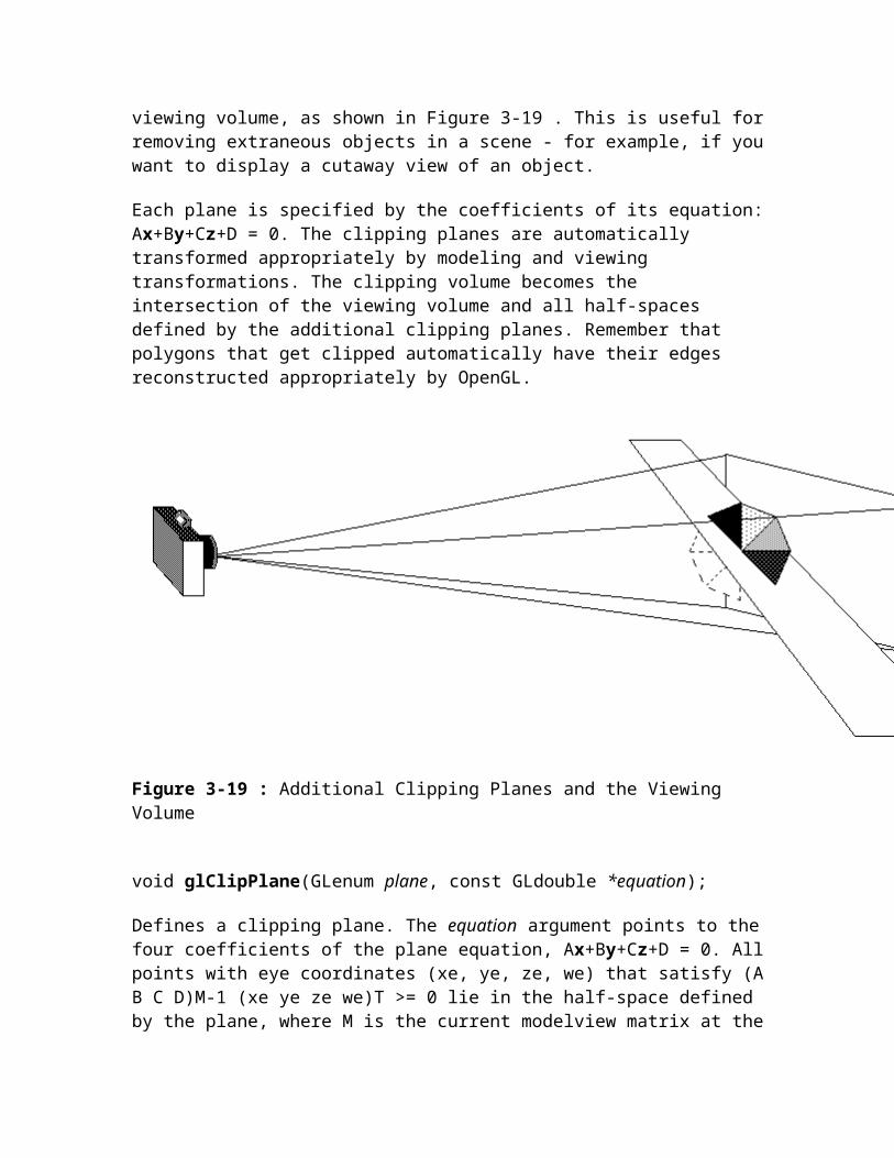
Sets the current red, green, blue, and alpha values. This command can have up to three suffixes, which differentiate variations of the parameters accepted. The first suffix is either 3 or 4, to indicate whether you supply an alpha value in addition to the red, green, and blue values. If you don't supply an alpha value, it's automatically set to 1.0. The second suffix indicates the data type for parameters: byte, short, integer, float, double, unsigned byte, unsigned short, or unsigned integer. The third suffix is an optional v, which indicates that the argument is a pointer to an array of values of the given data type.

For the versions of glColor*() that accept floating-point data types, the values should typically range between 0.0 and 1.0, the minimum and maximum values that can be stored in the framebuffer. (Values ouside the range [0,1] are clamped to the range [0,1] when used directly, but aren't clamped when used to modify lighting material parameters.) Unsigned-integer color components, when specified, are linearly mapped to floating-point values such that the largest representable value maps to 1.0 (full intensity), and zero maps to 0.0 (zero intensity). Signed-integer color components, when specified, are linearly mapped to floating-point values such that the most positive representable value maps to 1.0, and the most negative representable value maps to -1.0 (see Table 5-1 ). Floating-point values are mapped directly. Neither floating-point nor signed-integer values are clamped to the range [0,1] before updating the current color. However, color components are clamped to this range before they are interpolated or written into a color buffer.

Table 5-1 : Converting Color Values to Floating-Point Numbers

Suffix Data Type Minimum Value

Min Value

Maps to

Maximum Value

Max Value

Maps to

b 1-byte integer

-128 -1.0 127 1.0

s 2-byte integer

-32,768 -1.0 32,767 1.0

i 4-byte integer

-2,147,483,648 -1.0 2,147,483,647 1.0

ub unsigned 1-byte integer

0 0.0 255 1.0

us unsigned 2-byte integer

0 0.0 65,535 1.0

ui unsigned 4-byte integer

0 0.0 4,294,967,295 1.0

Specifying a Color in Color-Index Mode

In color-index mode, use the glIndex*() command to select a single-valued color index as the current color index. void glIndex{sifd}(TYPE c); void glIndex{sifd}v(const TYPE *c);

Sets the current color index. The first suffix for this command indicates the data type for parameters: short, integer, float, or double. The second, optional suffix is v, which indicates that the argument is an array of values of the given data type (the array contains only one value).

Advanced

The current index is stored as a floating-point value. Integer values are converted directly to floating-point values, with no special mapping. Index values outside the representable range of the color-index buffer aren't clamped. However, before an index is dithered (if enabled) and written to the framebuffer, it's converted to fixed-point format. Any bits in the integer portion of the resulting fixed-point value that don't correspond to bits in the framebuffer are masked out.

Specifying a Shading Model

A line or a filled polygon primitive can be drawn with a single color (flat shading) or with many different colors (smooth shading, also called Gouraud shading). You specify the desired shading technique with glShadeModel().void glShadeModel (GLenum mode);

Sets the shading model. The mode parameter can be either GL_SMOOTH (the default) or GL_FLAT.

With flat shading, the color of one vertex of a primitive is duplicated across all the primitive's vertices. With smooth shading, the color at each vertex is treated individually. For a line primitive, the colors along the line segment are interpolated between the vertex colors. For a polygon primitive, the colors for the interior of the polygon are interpolated between the vertex colors. Example 5-1 draws a smooth-shaded triangle, as shown in Figure J-11 .

Example 5-1 : Drawing a Smooth-Shaded Triangle: smooth.c

#include <GL/gl.h>#include <GL/glu.h>#include "aux.h"

void myinit (void){    glShadeModel (GL_SMOOTH);   /* GL_SMOOTH is the default */}

void triangle(void){    glBegin (GL_TRIANGLES);        glColor3f (1.0, 0.0, 0.0);        glVertex2f (5.0, 5.0);        glColor3f (0.0, 1.0, 0.0);        glVertex2f (25.0, 5.0);        glColor3f (0.0, 0.0, 1.0);        glVertex2f (5.0, 25.0);    glEnd ();}

void display(void){    glClear (GL_COLOR_BUFFER_BIT);    triangle ();    glFlush ();}

void myReshape(GLsizei w, GLsizei h){    glViewport(0, 0, w, h);    glMatrixMode(GL_PROJECTION);    glLoadIdentity();    if (w <= h)         gluOrtho2D (0.0, 30.0, 0.0,              30.0 * (GLfloat) h/(GLfloat) w);    else         gluOrtho2D (0.0, 30.0 * (GLfloat) w/(GLfloat) h, 0.0,             30.0);    glMatrixMode(GL_MODELVIEW);}

int main(int argc, char** argv){    auxInitDisplayMode (AUX_SINGLE | AUX_RGBA);    auxInitPosition (0, 0, 500, 500);    auxInitWindow (argv[0]);    myinit();    auxReshapeFunc (myReshape);    auxMainLoop(display);}With smooth shading, neighboring pixels have slightly different color values. In RGBA mode, adjacent pixels with slightly different values look similar, so the color changes across a polygon appear gradual. In color-index mode, adjacent pixels may reference different locations in the color-index table, which may not have similar colors at all. Adjacent color-index entries may contain wildly different colors, so a smooth-shaded polygon in color-index mode can look psychedelic.

To avoid this problem, you have to create a color ramp of smoothly changing colors among a contiguous set of indices in the color map. Remember that loading colors into a color map is performed through your window system rather than OpenGL. For the moment, however, assume you have an auxSetOneColor() routine that loads a single index in the color map with specified red, green, and blue values. The first argument for this routine is the index, and the others are the red, green, and blue values. To load thirty-two contiguous color indices (from color index 16 to 47) with slightly differing shades of yellow, you might call

for(i=0; i<32; i++){   auxSetOneColor(16+i, 1.0*(i/32.0), 1.0*(i/32.0), 0.0);}Now, if you render smooth-shaded polygons that use only the colors from index 16 to 47, those polygons have gradually differing shades of yellow.

With flat shading, the color of a single vertex defines the color of an entire primitive. For a line segment, the color of the line is the current color when the second (ending) vertex is specified. For a polygon, the color used is the one that's in effect when a particular vertex is specified, as shown in Table 5-2 . The table counts vertices and polygons starting from 1. OpenGL follows these rules consistently, but the best way to avoid uncertainty about how a flat-shaded primitive will be drawn is to specify only one color for the primitive.

Table 5-2 : How OpenGL Selects a Color for the ith Flat-Shaded Polygon

Type of Polygon Vertex Used to Select the Color for the ith Polygon

single polygon 1

triangle strip i+2

triangle fan i+2

independent triangle 3i

quad strip 2i+2

independent quad 4i

[Previous chapter] [Next chapter]

See the About page for copyright, authoring and distribution information.

Chapter 6LightingChapter Objectives

After reading this chapter, you'll be able to do the following:

Understand how real-world lighting conditions are approximated by OpenGL  

Render illuminated objects by defining the desired light sources and lighting model  

Define the material properties of the objects being illuminated  

Manipulate the matrix stack to control the position of light sources

As you saw in Chapter 5 , OpenGL computes the color of each pixel in a final, displayed scene that's held in the framebuffer. Part of this computation depends on what lighting is used in the scene and on how objects in the scene reflect or absorb that light. As an example of this, recall that the ocean has a different color on a bright, sunny day than it does on a gray, cloudy day. The presence of sunlight or clouds determines whether you see the ocean as bright turquoise or murky gray-green. In fact, most objects don't even look three-dimensional until they're lit. Figure 6-1 shows two versions of the exact same scene (a single sphere), one with lighting and one without.

Figure 6-1 : A Lit and an Unlit Sphere    

As you can see, an unlit sphere looks no different from a two-dimensional disk. This demonstrates how critical the interaction between objects and light is in creating a three-dimensional scene.

With OpenGL, you can manipulate the lighting and objects in a scene to create many different kinds of effects. This chapter explains how to control the lighting in a scene. It discusses OpenGL's conceptual model of lighting, and it describes in detail how to set the numerous illumination parameters to achieve certain effects. Toward the end of the chapter, the mathematical computations that determine how lighting affects color are presented.

This chapter contains the following major sections:

"Real-World and OpenGL Lighting" explains in general terms how light behaves in the world and how OpenGL models this behavior.  

"A Simple Example: Rendering a Lit Sphere" introduces OpenGL's lighting facility by presenting a short program that renders a lit sphere.  

"Creating Light Sources" explains how to define and position light sources.  

"Selecting a Lighting Model" discusses the elements of a lighting model and how to specify them.  

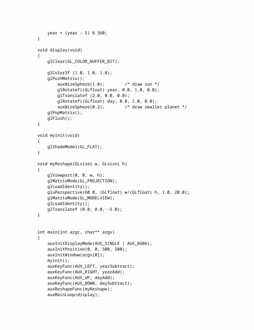
"Defining Material Properties" explains how to describe the properties of objects so that they interact with light in a desired way.  

"The Mathematics of Lighting" presents the mathematical calculations used by OpenGL to determine the effect of lights in a scene.  

"Lighting in Color-Index Mode" discusses the differences between using RGBA mode and color-index mode for lighting.

Real-World and OpenGL LightingWhen you look at a physical surface, your eye's perception of the color depends on the distribution of photon energies that arrive and trigger your cone cells, as described in "Color Perception." Those photons come from a light source or combination of sources, some of which are absorbed and some of which are reflected by the surface. In addition, different surfaces may have very different properties - some are shiny, and preferentially reflect light in certain directions, while others scatter incoming light equally in all directions. Most surfaces are somewhere in between.

OpenGL approximates light and lighting as if light can be broken into red, green, and blue components. Thus, the color of light sources is characterized by the amount of red, green, and blue light they emit, and the material of surfaces is characterized by the percentage of the incoming red, green, and blue components that are reflected in various directions. The OpenGL lighting equations are just an approximation, but one that works fairly well and can be computed relatively quickly. If you desire a more accurate (or just different) lighting model, you have to do your own calculations in software. Such software can be enormously complex, as a few hours of reading any optics textbook should convince you.

In the OpenGL lighting model, the light in a scene comes from several light sources that can individually be turned on and off. Some light comes from a particular direction or position, and some light is generally scattered about the scene. For example, when you turn on a light bulb in a room, most of the light comes from the bulb, but some light comes after bouncing off one, two, three, or more walls. This bounced light (called ambient) is assumed to be so scattered that there is no way to tell its original direction, but it disappears if a particular light source is turned off.

Finally, there might be a general ambient light in the scene that comes from no particular source, as if it had been scattered so many times that its original source is impossible to determine.

In the OpenGL model, the light sources have an effect only when there are surfaces that absorb and reflect light. Each surface is assumed to be composed of a material with various properties. A material might emit its own light (like headlights on an automobile), it might scatter some incoming light in all directions, and it might reflect some portion of the incoming light in a preferential direction like a mirror or shiny surface.

The OpenGL lighting model considers the lighting to be divided into four independent components: emitted, ambient, diffuse, and specular. All four components are computed independently, and then added together.

Emitted, Ambient, Diffuse, and Specular Light

Emitted light is the simplest - it originates from an object and is unaffected by any light sources.

The ambient component is the light from that source that's been scattered so much by the environment that its direction is impossible to determine - it seems to come from all directions. Backlighting in a room has a large ambient component, since most of the light that reaches your eye has bounced off many surfaces first. A spotlight outdoors has a tiny ambient component; most of the light travels in the same direction, and since you're outdoors, very little of the light reaches your eye after bouncing off other objects. When ambient light strikes a surface, it's scattered equally in all directions.

Diffuse light comes from one direction, so it's brighter if it comes squarely down on a surface than if it barely glances off the surface. Once it hits a surface, however, it's scattered equally in all directions, so it appears equally bright, no matter where the eye is located. Any light coming from a particular position or direction probably has a diffuse component.

Finally, specular light comes from a particular direction, and it tends to bounce off the surface in a preferred direction. A well-collimated laser beam bouncing off a high-quality mirror produces almost 100 percent specular reflection. Shiny metal or plastic has a high specular component, and chalk or carpet has almost none. You can think of specularity as shininess.

Although a light source delivers a single distribution of frequencies, the ambient, diffuse, and specular components might be different. For example, if you have a white light in a room with red walls, the scattered light tends to be red, although the light directly striking objects is white. OpenGL allows you to set the red, green, and blue values for each component of light independently.

Material Colors

The OpenGL lighting model makes the approximation that a material's color depends on the percentages of the incoming red, green, and blue light it reflects. For example, a

perfectly red ball reflects all the incoming red light and absorbs all the green and blue light that strikes it. If you view such a ball in white light (composed of equal amounts of red, green, and blue light), all the red is reflected, and you see a red ball. If the ball is viewed in pure red light, it also appears to be red. If, however, the red ball is viewed in pure green light, it appears black (all the green is absorbed, and there's no incoming red, so no light is reflected).

Like lights, materials have different ambient, diffuse, and specular colors, which determine the ambient, diffuse, and specular reflectances of the material. A material's ambient reflectance is combined with the ambient component of each incoming light source, the diffuse reflectance with the light's diffuse component, and similarly for the specular reflectance and component. Ambient and diffuse reflectances define the color of the material and are typically similar if not identical. Specular reflectance is usually white or gray, so that specular highlights end up being the color of the light source's specular intensity. If you think of a white light shining on a shiny red plastic sphere, most of the sphere appears red, but the shiny highlight is white.

RGB Values for Lights and Materials

The color components specified for lights mean something different than for materials. For a light, the numbers correspond to a percentage of full intensity for each color. If the R, G, and B values for a light's color are all 1.0, the light is the brightest possible white. If the values are 0.5, the color is still white, but only at half intensity, so it appears gray. If R=G=1 and B=0 (full red and green with no blue), the light appears yellow.

For materials, the numbers correspond to the reflected proportions of those colors. So if R=1, G=0.5, and B=0 for a material, that material reflects all the incoming red light, half the incoming green, and none of the incoming blue light. In other words, if an OpenGL light has components (LR, LG, LB), and a material has corresponding components (MR, MG, MB), then, ignoring all other reflectivity effects, the light that arrives at the eye is given by (LR*MR, LG*MG, LB*MB).

Similarly, if you have two lights, which send (R1, G1, B1) and (R2, G2, B2) to the eye, OpenGL adds the components, giving (R1+R2, G1+G2, B1+B2). If any of the sums are greater than 1 (corresponding to a color brighter than the equipment can display), the component is clamped to 1.

A Simple Example: Rendering a Lit SphereThese are the steps required to add lighting to your scene:

Define normal vectors for each vertex of all the objects. These normals determine the orientation of the object relative to the light sources.  

Create, select, and position one or more light sources.  

Create and select a lighting model, which defines the level of global ambient light and the effective location of the viewpoint (for the purposes of lighting calculations).  

Define material properties for the objects in the scene.

Example 6-1 accomplishes these tasks. It displays a sphere illuminated by a single light source, as shown earlier in Figure 6-1 .

Example 6-1 : Drawing a Lit Sphere:

#include <GL/gl.h>#include <GL/glu.h>#include "aux.h"

void myinit(void){    GLfloat mat_specular[] = { 1.0, 1.0, 1.0, 1.0 };    GLfloat mat_shininess[] = { 50.0 };    GLfloat light_position[] = { 1.0, 1.0, 1.0, 0.0 };

    glMaterialfv(GL_FRONT, GL_SPECULAR, mat_specular);    glMaterialfv(GL_FRONT, GL_SHININESS, mat_shininess);    glLightfv(GL_LIGHT0, GL_POSITION, light_position);

    glEnable(GL_LIGHTING);    glEnable(GL_LIGHT0);    glDepthFunc(GL_LEQUAL);    glEnable(GL_DEPTH_TEST);}

void display(void){    glClear(GL_COLOR_BUFFER_BIT | GL_DEPTH_BUFFER_BIT);    auxSolidSphere(1.0);    glFlush();}

void myReshape(GLsizei w, GLsizei h){    glViewport(0, 0, w, h);    glMatrixMode(GL_PROJECTION);    glLoadIdentity();    if (w <= h)         glOrtho (-1.5, 1.5, -1.5*(GLfloat)h/(GLfloat)w,             1.5*(GLfloat)h/(GLfloat)w, -10.0, 10.0);    else         glOrtho (-1.5*(GLfloat)w/(GLfloat)h,             1.5*(GLfloat)w/(GLfloat)h, -1.5, 1.5, -10.0, 10.0);

    glMatrixMode(GL_MODELVIEW);    glLoadIdentity();}

int main(int argc, char** argv){    auxInitDisplayMode (AUX_SINGLE | AUX_RGBA | AUX_DEPTH);    auxInitPosition (0, 0, 500, 500);    auxInitWindow (argv[0]);    myinit();    auxReshapeFunc (myReshape);    auxMainLoop(display);}The lighting-related calls are in the myinit() command; they're discussed briefly in the following paragraphs and in more detail later in the chapter. One thing to note about Example 6-1 is that it uses RGBA color mode, not color-index mode. OpenGL's lighting calculation is different for the two modes, and in fact the lighting capabilities are more limited in color-index mode. Thus, RGBA is the preferred mode when doing lighting, and all the examples in this chapter use it. See "Lighting in Color-Index Mode" for more information about lighting in color-index mode.

Define Normal Vectors for Each Vertex of All the Objects

An object's normals determine its orientation relative to the light sources. For each vertex, OpenGL uses the assigned normal to determine how much light that particular vertex receives from each light source. In this example, the normals for the sphere are defined as part of the auxSolidSphere() routine. See "Normal Vectors" for more details on how to define normals.

Create, Position, and Enable One or More Light Sources

Example 6-1 uses only one, white light source; its location is specified by the glLightfv() call. This example uses the default color for light zero (GL_LIGHT0), which is white; if you had wanted a differently colored light, you'd use glLight*() to indicate this. You can include at least eight different light sources in your scene of various colors; the default color of these other lights is black. (The particular implementation of OpenGL you're using might allow more than eight.) You can also locate the lights wherever you desire - you can position them near the scene, as a desk lamp would be, or an infinite distance away, like the sun. In addition, you can control whether a light produces a narrow, focused beam or a wider beam. Remember that each light source adds significantly to the calculations needed to render the scene, so performance is affected by the number of lights in the scene. See "Creating Light Sources" for more information about how to create lights with the desired characteristics.

After you've defined the characteristics of the lights you want, you have to turn them on with the glEnable() command. You also need to call this command with GL_LIGHTING as a parameter to prepare OpenGL to perform lighting calculations. See "Enabling Lighting" for more information about how to do this.

Select a Lighting Model

As you might expect, the glLightModel*() command describes the parameters of a lighting model. In Example 6-1 , the only element of the lighting model that's defined explicitly is the global ambient light. The lighting model also defines whether the viewer of the scene should be considered to be an infinite distance away or local to the scene, and whether lighting calculations should be performed differently for the front and back surfaces of objects in the scene. Example 6-1 uses the default settings for these two aspects of the model - an infinite viewer and one-sided lighting. Using a local viewer adds significantly to the complexity of the calculations that must be performed because OpenGL must calculate the angle between the viewpoint and each object. With an infinite viewer, however, the angle is ignored, and the results are slightly less realistic. Further, since in this example, the back surface of the sphere is never seen (it's the inside of the sphere), one-sided lighting is sufficient. The section "Selecting a Lighting Model" describes the elements of an OpenGL lighting model in more detail.

Define Material Properties for the Objects in the Scene

An object's material properties determine how it reflects light and therefore what material it seems to be made of. Because the interaction between an object's material surface and incident light is complex, specifying material properties so that an object has a certain desired appearance is an art. You can specify a material's ambient, diffuse, and specular colors and how shiny it is. In this example, only these last two material properties - the specular material color and shininess - are explicitly specified (with the glMaterialfv() calls). "Defining Material Properties" describes and gives examples of all the material-property parameters.

Some Important Notes

As you write your own lighting program, remember that you can use the default values for some lighting parameters; others need to be changed. Also, don't forget to enable whatever lights you define and to enable lighting calculations. Finally, remember that you might be able to use display lists to maximize efficiency as you change lighting conditions; see "Display-List Design Philosophy."

Creating Light SourcesLight sources have a number of properties, such as color, position, and direction. The following sections explain how to control these properties and what the resulting light looks like. The command used to specify all properties of lights is glLight*(); it takes three arguments: to identify the light whose property is being specified, the property, and

the desired value for that property. void glLight{if}[v](GLenum light, GLenum pname, TYPEparam);

Creates the light specified by light, which can be GL_LIGHT0, GL_LIGHT1, ... , or GL_LIGHT7. The characteristic of the light being set is defined by pname, which specifies a named parameter (see Table 6-1 ). The param argument indicates the values to which the pname characteristic is set; it's a pointer to a group of values if the vector version is used, or the value itself if the nonvector version is used. The nonvector version can be used to set only single-valued light characteristics.

Table 6-1 : Default Values for pname Parameter of glLight*()

Parameter Name Default Value Meaning

GL_AMBIENT (0.0, 0.0, 0.0, 1.0)

ambient RGBA intensity of light

GL_DIFFUSE (1.0, 1.0, 1.0, 1.0)

diffuse RGBA intensity of light

GL_SPECULAR (1.0, 1.0, 1.0, 1.0)

specular RGBA intensity of light

GL_POSITION (0.0, 0.0, 1.0, 0.0)

(x, y, z, w) position of light

GL_SPOT_DIRECTION (0.0, 0.0, -1.0) (x, y, z) direction of spotlight

GL_SPOT_EXPONENT 0.0 spotlight exponent

GL_SPOT_CUTOFF 180.0 spotlight cutoff angle

GL_CONSTANT_ATTENUATION 1.0 constant attenuation factor

GL_LINEAR_ATTENUATION 0.0 linear attenuation factor

GL_QUADRATIC_ATTENUATION 0.0 quadratic attenuation factor

 

The default values listed for GL_DIFFUSE and GL_SPECULAR in Table 6-1 apply only to GL_LIGHT0. For other lights, the default value is (0.0, 0.0, 0.0, 1.0) for both GL_DIFFUSE and GL_SPECULAR.

Here's an example of using glLight*():

GLfloat light_ambient[] = { 0.0, 0.0, 0.0, 1.0 };GLfloat light_diffuse[] = { 1.0, 1.0, 1.0, 1.0 };GLfloat light_specular[] = { 1.0, 1.0, 1.0, 1.0 };GLfloat light_position[] = { 1.0, 1.0, 1.0, 0.0 };

glLightfv(GL_LIGHT0, GL_AMBIENT, light_ambient);glLightfv(GL_LIGHT0, GL_DIFFUSE, light_diffuse);glLightfv(GL_LIGHT0, GL_SPECULAR, light_specular);glLightfv(GL_LIGHT0, GL_POSITION, light_position);As you can see, arrays are defined for the parameter values, and glLightfv() is called repeatedly to set the various parameters. In this example, the first three calls to glLightfv() are superfluous, since they're being used to specify the default values for the GL_AMBIENT, GL_DIFFUSE, and GL_SPECULAR parameters.

Remember to turn on each light with glEnable(); see "Enabling Lighting" for more information about how to do this.

All the parameters for glLight*() and their possible values are explained in the following sections. These parameters interact with those that define the overall lighting model for a particular scene and an object's material properties. See "Selecting a Lighting Model" and "Defining Material Properties" for more information about these two topics. "The Mathematics of Lighting" explains how all these parameters interact mathematically.

Color

OpenGL allows you to associate three different color-related parameters - GL_AMBIENT, GL_DIFFUSE, and GL_SPECULAR - with any particular light. The GL_AMBIENT parameter refers to the RGBA intensity of the ambient light that a particular light source adds to the scene. As you can see in Table 6-1 , by default there is no ambient light since GL_AMBIENT is (0.0, 0.0, 0.0, 1.0). This value was used in Example 6-1 . If this program had specified blue ambient light GLfloat light_ambient[] = { 0.0, 0.0, 1.0, 1.0};glLightfv(GL_LIGHT0, GL_AMBIENT, light_ambient);the result would have been as shown in the left part of Figure J-14 .

The GL_DIFFUSE parameter probably most closely correlates with what you naturally think of as "the color of a light." It defines the RGBA color of the diffuse light that a particular light source adds to a scene. By default, GL_DIFFUSE is (1.0, 1.0, 1.0, 1.0) for GL_LIGHT0, which produces a bright, white light as shown in Figure J-14 . The default value for any other light (GL_LIGHT1, ... , GL_LIGHT7) is (0.0, 0.0, 0.0, 0.0).

The GL_SPECULAR parameter affects the color of the specular highlight on an object. Typically, a real-world object such as a glass bottle has a specular highlight that's the color of the light shining on it (which is often white). Therefore, if you want to create a realistic effect, set the GL_SPECULAR parameter to the same value as the GL_DIFFUSE parameter. By default, GL_SPECULAR is (1.0, 1.0, 1.0, 1.0) for GL_LIGHT0 and (0.0, 0.0, 0.0, 0.0) for any other light.

Position and Attenuation

As previously mentioned, you can choose whether to have a light source that's treated as though it's located infinitely far away from the scene or one that's nearer to the scene. The first type is referred to as an directional light source; the effect of an infinite location is that the rays of light can be considered parallel by the time they reach an object. An example of a real-world directional light source is the sun. The second type is called a positional light source, since its exact position within the scene determines the effect it has on a scene and, specifically, the direction from which the light rays come. A desk lamp is an example of a positional light source. You can see the difference between directional and positional lights in Figure J-16 .

The light used in Example 6-1 is a directional one:

GLfloat light_position[] = { 1.0, 1.0, 1.0, 0.0 };glLightfv(GL_LIGHT0, GL_POSITION, light_position);As shown, you supply a vector of four values (x, y, z, w) for the GL_POSITION parameter. If the last value, w, is zero, the corresponding light source is a directional one, and the (x, y, z) values describe its direction. This direction is transformed by the modelview matrix just as it would be if it described a normal vector. By default, GL_POSITION is (0, 0, 1, 0), which defines a directional light that points along the negative z-axis. (Note that nothing prevents you from creating a directional light with the direction of (0, 0, 0), but such a light won't help you much.)

If the w value is nonzero, the light is positional, and the (x, y, z) values specify the location of the light in homogeneous object coordinates (see Appendix G ). This location is transformed by the modelview matrix and stored in eye coordinates. See "Controlling a Light's Position and Direction" for more information about how to control the transformation of the light's location. Also, by default, a positional light radiates in all directions, but you can restrict it to producing a cone of illumination by defining the light as a spotlight. The next section, "Spotlights," explains how to define a light as a spotlight.

Remember that the colors across the face of a smooth-shaded polygon are determined by the colors calculated for the vertices. Because of this, you probably want to avoid using large polygons with local lights - if you locate the light near the middle of the polygon, the vertices might be too far away to receive much light, so the whole polygon will look darker than you intended. To avoid this problem, break up the large polygon into smaller ones.

For real-world lights, the intensity of light decreases as distance from the light increases. Since a directional light is infinitely far away, it doesn't make sense to attenuate its intensity over distance, so attenuation is disabled for a directional light. However, you might want to attenuate the light from a positional light. OpenGL attenuates a light source by multiplying the contribution of that source by an attenuation factor:

where

d = distance between the light's position and the vertex

kc = GL_CONSTANT_ATTENUATION

kl = GL_LINEAR_ATTENUATION

kq = GL_QUADRATIC_ATTENUATION

By default, kc is 1.0 and both kl and kq are zero, but you can give these parameters different values:

glLightf(GL_LIGHT0, GL_CONSTANT_ATTENUATION, 2.0);glLightf(GL_LIGHT0, GL_LINEAR_ATTENUATION, 1.0);glLightf(GL_LIGHT0, GL_QUADRATIC_ATTENUATION, 0.5);Note that the ambient, diffuse, and specular contributions are all attenuated. Only the emission and global ambient values aren't attenuated.

Spotlights

As previously mentioned, you can have a positional light source act as a spotlight - that is, by restricting the shape of the light it emits to a cone. To create a spotlight, you need to determine the spread of the cone of light you desire. (Remember that since spotlights are positional lights, you also have to locate them where you want them. Again, note that nothing prevents you from creating a directional spotlight, but it probably won't give you the result you want.) To specify the angle between the axis of the cone and a ray along the edge of the cone, use the GL_SPOT_CUTOFF parameter. The angle of the cone at the apex is then twice this value, as shown in Figure 6-2 .

Figure 6-2 : The GL_SPOT_CUTOFF Parameter    

Note that no light is emitted beyond the edges of the cone. By default, the spotlight feature is disabled because the GL_SPOT_CUTOFF parameter is 180.0. This value means that light is emitted in all directions (the angle at the cone's apex is 360 degrees, so it isn't a cone at all). The value for GL_SPOT_CUTOFF is restricted to being within the range [0.0,90.0] (unless it has the special value 180.0). The following line sets the cutoff parameter to 45 degrees:

glLightf(GL_LIGHT0, GL_SPOT_CUTOFF, 45.0);You also need to specify a spotlight's direction, which determines the axis of the cone of light: GLfloat spot_direction[] = { -1.0, -1.0, 0.0 };glLightfv(GL_LIGHT0, GL_SPOT_DIRECTION, spot_direction);The direction is specified in homogeneous object coordinates. By default, the direction is (0.0, 0.0, -1.0), so if you don't explicitly set the value of GL_SPOT_DIRECTION, the light points down the negative z-axis. Also, keep in mind that a spotlight's direction is transformed by the modelview matrix just as though it were a normal vector, and the result is stored in eye coordinates. (See "Controlling a Light's Position and Direction" for more information about such transformations.)

In addition to the spotlight's cutoff angle and direction, you can control the intensity distribution of the light within the cone, in two ways. First, you can set the attenuation factor described earlier, which is multiplied by the light's intensity. You can also set the GL_SPOT_EXPONENT parameter, which is by default zero, to control how concentrated the light is. The light's intensity is highest in the center of the cone. It's attenuated toward the edges of the cone by the cosine of the angle between the direction of the light and the direction from the light to the vertex being lighted, raised to the power of the spot exponent. Thus, higher spot exponents result in a more focused light source. See "The Mathematics of Lighting" for more details on the equations used to calculate light intensity.

Multiple Lights

As mentioned, you can have at least eight lights in your scene (possibly more, depending on your OpenGL implementation). Since OpenGL needs to perform calculations to determine how much light each vertex receives from each light source, increasing the number of lights adversely affects performance. The constants used to refer to the eight lights are GL_LIGHT0, GL_LIGHT1, GL_LIGHT2, GL_LIGHT3, and so on. In the preceding discussions, parameters related to GL_LIGHT0 were set. If you want an additional light, you need to specify its parameters; also, remember that the default values are different for these other lights than they are for GL_LIGHT0, as explained in Table 6-1 . The following lines of code define a white attenuated spotlight: GLfloat light1_ambient[] = { 0.2, 0.2, 0.2, 1.0 };GLfloat light1_diffuse[] = { 1.0, 1.0, 1.0, 1.0 };GLfloat light1_specular[] = { 1.0, 1.0, 1.0, 1.0 };GLfloat light1_position[] = { -2.0, 2.0, 1.0, 1.0 };GLfloat spot_direction[] = { -1.0, -1.0, 0.0 };

glLightfv(GL_LIGHT1, GL_AMBIENT, light1_ambient);glLightfv(GL_LIGHT1, GL_DIFFUSE, light1_diffuse);glLightfv(GL_LIGHT1, GL_SPECULAR, light1_specular);glLightfv(GL_LIGHT1, GL_POSITION, light1_position);glLightf(GL_LIGHT1, GL_CONSTANT_ATTENUATION, 1.5);glLightf(GL_LIGHT1, GL_LINEAR_ATTENUATION, 0.5);glLightf(GL_LIGHT1, GL_QUADRATIC_ATTENUATION, 0.2);

glLightf(GL_LIGHT1, GL_SPOT_CUTOFF, 45.0);glLightfv(GL_LIGHT0, GL_SPOT_DIRECTION, spot_direction);glLightf(GL_LIGHT1, GL_SPOT_EXPONENT, 2.0);

glEnable(GL_LIGHT1);If these lines were added to Example 6-1 , the sphere would be lit with two lights, one directional and one spotlight.

Try This

Try This

Modify Example 6-1 :

Change the light to be a positional colored light rather than a directional white one.  

Add an additional colored spotlight. Hint: Use some of the code shown in the preceding section.  

Measure how these two changes affect performance.

Controlling a Light's Position and Direction

OpenGL treats the position and direction of a light source just as it treats the position of a geometric primitive. In other words, a light source is subject to the same matrix transformations as a primitive. More specifically, when glLight*() is called to specify the position or the direction of a light source, the position or direction is transformed by the current modelview matrix and stored in eye coordinates. This means you can manipulate a light source's position or direction by changing the contents of the modelview matrix stack. (The projection matrix has no effect on a light's position or direction.) This section explains how to achieve three different effects by changing the point in the program at which the light position is set, relative to modeling or viewing transformations:

A light position that remains fixed  

A light that moves around a stationary object  

A light that moves along with the viewpoint

In the simplest example, as in Example 6-1 , the light position remains fixed. To achieve this effect, you need to set the light position after whatever viewing and/or modeling transformation you use. Here's what the relevant code from the myinit() and myReshape() routines might look like: glViewport(0, 0, w, h);glMatrixMode (GL_PROJECTION);glLoadIdentity();if (w <= h)     glOrtho (-1.5, 1.5, -1.5*h/w, 1.5*h/w, -10.0, 10.0);else     glOrtho (-1.5*w/h, 1.5*w/h, -1.5, 1.5, -10.0, 10.0);glMatrixMode (GL_MODELVIEW);glLoadIdentity();

/* later in myInit() */GLfloat light_position[] = { 1.0, 1.0, 1.0, 1.0 };glLightfv(GL_LIGHT0, GL_POSITION, position);As you can see, the viewport and projection matrices are established first. Then, the identity matrix is loaded as the modelview matrix, after which the light position is set. Since the identity matrix is used, the originally specified light position (1.0, 1.0, 1.0) isn't changed by being multiplied by the modelview matrix. Then, since neither the light position nor the modelview matrix is modified after this point, the light remains pointing at (1.0, 1.0, 1.0).

Now suppose you want to rotate or translate the light position so that the light moves relative to a stationary object. One way to do this is to set the light position after the modeling transformation, which is itself changed specifically to modify the light position. You can begin with the same series of calls in an init() routine early in the program. Then, probably within an event loop, you need to perform the desired modeling transformation (on the modelview stack) and reset the light position. Here's what such code might look like:

void display(GLint spin){    GLfloat light_position[] = { 0.0, 0.0, 1.5, 1.0 };    glClear(GL_COLOR_BUFFER_BIT | GL_DEPTH_BUFFER_BIT);

    glPushMatrix();        glTranslatef(0.0, 0.0, -5.0);         glPushMatrix();            glRotated((GLdouble) spin, 1.0, 0.0, 0.0);            glLightfv(GL_LIGHT0, GL_POSITION, light_position);        glPopMatrix();        auxSolidTorus();    glPopMatrix();    glFlush();}This display() command causes the scene to be redrawn with the light rotated spin degrees around a stationary torus. Note the two pairs of glPushMatrix() and glPopMatrix() calls, which are used to isolate the viewing and modeling transformations, all of which occur on the modelview stack. Since in this example the viewpoint remains constant, the current matrix is pushed down the stack and then the desired viewing transformation is loaded with glTranslatef(). The matrix stack is pushed again before the modeling transformation glRotated() is specified. Then the light position is set in the new, rotated coordinate system so that the light itself appears to be rotated from its previous position. (Remember that the light position is stored in eye coordinates, which are obtained after transformation by the modelview matrix.) After the rotated matrix is popped off the stack, the torus is drawn.

To create a light that moves along with the viewpoint, you need to set the light position before the viewing transformation. Then, the viewing transformation affects both the light and the viewpoint in the same way. For this example, let's use a slightly different set of calls in the myinit() routine:

GLfloat light_position() = { 0.0, 0.0, 1.0, 1.0 };

glViewport(0, 0, w-1, h-1);glMatrixMode(GL_PROJECTION);glLoadIdentity();gluPerspective(40.0, (GLfloat) w/(GLfloat) h, 1.0, 100.0);glMatrixMode(GL_MODELVIEW);

glLightfv(GL_LIGHT0, GL_POSITION, light_position);Then, the display() routine that's called from the event loop to redraw the scene might look like this: void display(GLint spin){    glClear(GL_COLOR_BUFFER_MASK | GL_DEPTH_BUFFER_MASK);    glPushMatrix();        glTranslatef (0.0, 0.0, -5.0);        glRotatef ((GLfloat) spin, 1.0, 0.0, 0.0);        auxSolidTorus();    glPopMatrix();    glFlush();

}When the lighted torus is redrawn, both the light position and the viewpoint are moved spin degrees. Even though you haven't respecified the light position, the light moves because the eye coordinate system has changed.

Try This

Try This

Modify Example 6-2 :

Make the light translate past the object instead of rotating around it. Hint: Use glTranslated() rather than the first glRotated() in display(), and choose an appropriate value to use instead of spin.  

Change the attenuation so that the light decreases in intensity as it's moved away from the object. Hint: Add calls to glLight*() to set the desired attenuation parameters.

Example 6-2 : Moving a Light with Modeling Transformations: movelight.c

#include <GL/gl.h>#include <GL/glu.h>#include "aux.h"

static int spin = 0;

void movelight (AUX_EVENTREC *event){    spin = (spin + 30) % 360;}

void myinit (void){    glEnable(GL_LIGHTING);    glEnable(GL_LIGHT0);

    glDepthFunc(GL_LEQUAL);    glEnable(GL_DEPTH_TEST);}

void display(void){    GLfloat position[] = { 0.0, 0.0, 1.5, 1.0 };

    glClear (GL_COLOR_BUFFER_BIT | GL_DEPTH_BUFFER_BIT);    glPushMatrix ();        glTranslatef (0.0, 0.0, -5.0); 

        glPushMatrix ();            glRotated ((GLdouble) spin, 1.0, 0.0, 0.0);

            glRotated (0.0, 1.0, 0.0, 0.0);            glLightfv (GL_LIGHT0, GL_POSITION, position);            glTranslated (0.0, 0.0, 1.5);            glDisable (GL_LIGHTING);            glColor3f (0.0, 1.0, 1.0);            auxWireCube (0.1);            glEnable (GL_LIGHTING);        glPopMatrix ();

        auxSolidTorus (0.275, 0.85);    glPopMatrix ();    glFlush ();}

void myReshape(GLsizei w, GLsizei h){    glViewport(0, 0, w, h);    glMatrixMode(GL_PROJECTION);    glLoadIdentity();    gluPerspective(40.0, (GLfloat) w/(GLfloat) h, 1.0, 20.0);    glMatrixMode(GL_MODELVIEW);}

int main(int argc, char** argv){    auxInitDisplayMode (AUX_SINGLE | AUX_RGBA | AUX_DEPTH);    auxInitPosition (0, 0, 500, 500);    auxInitWindow (argv[0]);    myinit();    auxMouseFunc (AUX_LEFTBUTTON, AUX_MOUSEDOWN, movelight);    auxReshapeFunc (myReshape);    auxMainLoop(display);}

Selecting a Lighting ModelOpenGL's notion of a lighting model has three components:

The global ambient light intensity  

Whether the viewpoint position is local to the scene or whether it should be considered to be an infinite distance away  

Whether lighting calculations should be performed differently for both the front and back faces of objects

This section explains how to specify a lighting model. It also discusses how to enable lighting - that is, how to tell OpenGL that you want lighting calculations performed.

Global Ambient Light

As discussed earlier, each light source can contribute ambient light to a scene. In addition, there can be other ambient light that's not from any particular source. To specify the RGBA intensity of such global ambient light, use the GL_LIGHT_MODEL_AMBIENT parameter as follows: GLfloat lmodel_ambient[] = { 0.2, 0.2, 0.2, 1.0 };glLightModelfv(GL_LIGHT_MODEL_AMBIENT, lmodel_ambient);In this example, the values used for lmodel_ambient are the default values for GL_LIGHT_MODEL_AMBIENT. Since these numbers yield a small amount of white ambient light, even if you don't add a specific light source to your scene, you can still see the objects in the scene. Figure J-18 shows the effect of different amounts of global ambient light.

Local or Infinite Viewpoint

The location of the viewpoint affects the calculations for highlights produced by specular reflectance. More specifically, the intensity of the highlight at a particular vertex depends on the normal at that vertex, the direction from the vertex to the light source, and the direction from the vertex to the viewpoint. Keep in mind that the viewpoint isn't actually being moved by calls to lighting commands (you need to change the projection transformation, as described in "Projection Transformations" ); instead, different assumptions are made for the lighting calculations as if the viewpoint were moved.

With an infinite viewpoint, the direction between it and any vertex in the scene remains constant. A local viewpoint tends to yield more realistic results, but since the direction has to be calculated for each vertex, overall performance is decreased with a local viewpoint. By default, an infinite viewpoint is assumed. Here's how to change to a local viewpoint:

glLightModeli(GL_LIGHT_MODEL_LOCAL_VIEWER, GL_TRUE);This call places the viewpoint at (0, 0, 0) in eye coordinates. To switch back to an infinite viewpoint, pass in GL_FALSE as the argument.

Two-sided Lighting

Lighting calculations are performed for all polygons, whether they're front-facing or back-facing. Since you usually set up lighting conditions with the front-facing polygons in mind, however, the back-facing ones typically aren't correctly illuminated. In Example 6-1 where the object is a sphere, only the front faces are ever seen, since they're the ones on the outside of the sphere. So, in this case, it doesn't matter what the back-facing polygons look like. If the sphere was going to be cut away so that its inside surface would be visible, however, you might want to have the inside surface be fully lit according to the lighting conditions you've defined; you might also want to supply a different material description for the back faces. When you turn on two-sided lighting, as follows glLightModeli(LIGHT_MODEL_TWO_SIDE, GL_TRUE);

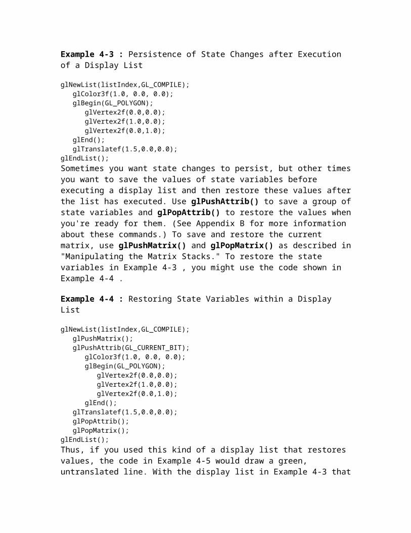
OpenGL reverses the surface normals for back-facing polygons; typically, this means that the surface normals of visible back- and front-facing polygons face the viewer, rather than pointing away. As a result, all polygons are illumnated correctly.

To turn two-sided lighting off, pass in GL_FALSE as the argument in the preceding call. See "Defining Material Properties" for information about how to supply material properties for both faces. You can also control which faces OpenGL considers to be front-facing with the command glFrontFace(). See "Reversing and Culling Polygon Faces" for more information about this command.

Enabling Lighting

With OpenGL, you need to explicitly enable (or disable) lighting. If lighting isn't enabled, the current color is simply mapped onto the current vertex, and no calculations concerning normals, light sources, the lighting model, and material properties are performed. Here's how to enable lighting: glEnable(GL_LIGHTING);To disable lighting, call glDisable() with GL_LIGHTING as the argument.

You also need to explicitly enable each light source that you define, after you've specified the parameters for that source. Example 6-1 uses only one light, GL_LIGHT0:

glEnable(GL_LIGHT0);

 

Defining Material PropertiesYou've seen how to create light sources with certain characteristics and how to define the desired lighting model. This section describes how to define the material properties of the objects in the scene: the ambient, diffuse, and specular colors, the shininess, and the color of any emitted light. The equations used in the lighting and material-property calculations are described in "The Mathematics of Lighting." Most of the material properties are conceptually similar to ones you've already used to create light sources. The mechanism for setting them is similar, except that the command used is called glMaterial*(). void glMaterial{if}[v](GLenum face, GLenum pname, TYPEparam);

Specifies a current material property for use in lighting calculations. The face parameter can be GL_FRONT, GL_BACK, or GL_FRONT_AND_BACK to indicate which face of the object the material should be applied to. The particular material property being set is identified by pname and the desired values for that property are given by param, which is either a pointer to a group of values (if the vector version is used) or the actual value (if the nonvector version is used). The nonvector version works only for setting GL_SHININESS. The possible values for pname are shown in Table 6-2 . Note that

GL_AMBIENT_AND_DIFFUSE allows you to set both the ambient and diffuse material colors simultaneously to the same RGBA value.

Table 6-2 : Default Values for pname Parameter of glMaterial*()

Parameter Name Default Value Meaning

GL_AMBIENT (0.2, 0.2, 0.2, 1.0)

ambient color of material

GL_DIFFUSE (0.8, 0.8, 0.8, 1.0)

diffuse color of material

GL_AMBIENT_AND_DIFFUSE ambient and diffuse color of material

GL_SPECULAR (0.0, 0.0, 0.0, 1.0)

specular color of material

GL_SHININESS 0.0 specular exponent

GL_EMISSION (0.0, 0.0, 0.0, 1.0)

emissive color of material

GL_COLOR_INDEXES (0,1,1) ambient, diffuse, and specular color indices

 

As discussed in "Selecting a Lighting Model," you can choose to have lighting calculations performed differently for the front- and back-facing polygons of objects. If the back faces might indeed be seen, you can supply different material properties for the front and the back surfaces by using the face parameter of glMaterial*(). See Figure J-19 for an example of an object drawn with different inside and outside material properties.

To give you an idea of the possible effects you can achieve by manipulating material properties, see Figure J-21 . This figure shows the same object drawn with several different sets of material properties. The same light source and lighting model are used for the entire figure. The sections that follow discuss the specific properties used to draw each of these spheres.

Note that most of the material properties set with glMaterial*() are (R, G, B, A) colors. Regardless of what alpha values are supplied for other parameters, the alpha value at any particular vertex is the diffuse-material alpha value (that is, the alpha value given to GL_DIFFUSE with the glMaterial*() command, as described in the next section. (See "Blending" for a complete discussion of alpha values.) Also, none of the RGBA material properties apply in color-index mode; see "Lighting in Color-Index Mode" for more information about what parameters are relevant in color-index mode.

Diffuse and Ambient Reflection

The GL_DIFFUSE and GL_AMBIENT parameters set with glMaterial*() affect the color of the diffuse and ambient light reflected by an object. Diffuse reflectance plays the most important role in determining what you perceive the color of an object to be. It's affected by the color of the incident diffuse light and the angle of the incident light relative to the normal direction. (It's most intense where the incident light falls perpendicular to the surface.) The position of the viewpoint doesn't affect diffuse reflectance at all.

Ambient reflectance affects the overall color of the object. Because diffuse reflectance is brightest where an object is directly illuminated, ambient reflectance is most noticeable where an object receives no direct illumination. An object's total ambient reflectance is affected by the global ambient light and ambient light from individual light sources. Like diffuse reflectance, ambient reflectance isn't affected by the position of the viewpoint.

For real-world objects, diffuse and ambient reflectance are normally the same color. For this reason, OpenGL provides you with a convenient way of assigning the same value to both simultaneously with glMaterial*():

GLfloat mat_amb_diff[] = { 0.1, 0.5, 0.8, 1.0 };glMaterialfv(GL_FRONT_AND_BACK, GL_AMBIENT_AND_DIFFUSE,             mat_amb_diff);In this example, the RGBA color (0.1, 0.5, 0.8, 1.0) - a deep blue color - represents the current ambient and diffuse reflectance for both the front- and back-facing polygons.

In Figure J-21 , the first row of spheres has no ambient reflectance (0.0, 0.0, 0.0, 0.0), and the second row has a significant amount of it (0.7, 0.7, 0.7, 1.0).

Specular Reflection

Specular reflection from an object produces highlights. Unlike ambient and diffuse reflection, the amount of specular reflection seen by a viewer does depend on the location of the viewpoint - it's brightest along the direct angle of reflection. To see this, imagine looking at a metallic ball outdoors in the sunlight. As you move your head, the highlight created by the sunlight moves with you to some extent. However, if you move your head too much, you lose the highlight entirely.

OpenGL allows you to set the RGBA color of a specular highlight (with GL_SPECULAR) and to control the size and brightness of the highlight (with GL_SHININESS). You can assign a number in the range of [0.0, 128.0] to GL_SHININESS - the higher the value, the smaller and brighter (more focused) the highlight. See "The Mathematics of Lighting" for the details of how specular highlights are calculated.

In Figure J-21 , the spheres in the first column have no specular reflection. In the second column, GL_SPECULAR and GL_SHININESS are assigned values as follows:

GLfloat mat_specular[] = { 1.0, 1.0, 1.0, 1.0 };GLfloat low_shininess[] = { 5.0 };glMaterialfv(GL_FRONT, GL_SPECULAR, mat_specular);glMaterialfv(GL_FRONT, GL_SHININESS, low_shininess);In the third column, the GL_SHININESS parameter is increased to 100.0.

Emission

By specifying an RGBA color for GL_EMISSION, you can make an object appear to be giving off light of that color. Since most real-world objects (except lights) don't emit light, you'll probably use this feature mostly to simulate lamps and other light sources in a scene. In Figure J-21 , the spheres in the fourth column have a greenish value for GL_EMISSION: GLfloat mat_emission[] = {0.3, 0.2, 0.2, 0.0};glMaterialfv(GL_FRONT, GL_EMISSION, mat_emission);Notice that the spheres appear to be slightly glowing; however, they're not actually acting as light sources. You would need to create a light source and position it at the same location as the sphere to create that effect.

Changing Material Properties

Example 6-1 uses the same material properties for all vertices of the only object in the scene (the sphere). In other situations, you might want to assign different material properties for different vertices on the same object. More likely, you have more than one object in the scene, and each object has different material properties. For example, the code that produced Figure J-21 has to draw eight different objects (all spheres), each with different material properties. Example 6-3 shows some of the code in the display() routine.

Example 6-3 : Using Different Material Properties: material.c

GLfloat no_mat[] = { 0.0, 0.0, 0.0, 1.0 };GLfloat mat_ambient[] = { 0.7, 0.7, 0.7, 1.0 };GLfloat mat_ambient_color[] = { 0.8, 0.8, 0.2, 1.0 };GLfloat mat_diffuse[] = { 0.1, 0.5, 0.8, 1.0 };GLfloat mat_specular[] = { 1.0, 1.0, 1.0, 1.0 };GLfloat no_shininess[] = { 0.0 };GLfloat low_shininess[] = { 5.0 };GLfloat high_shininess[] = { 100.0 };

GLfloat mat_emission[] = {0.3, 0.2, 0.2, 0.0};

glClear(GL_COLOR_BUFFER_BIT | GL_DEPTH_BUFFER_BIT);/* draw sphere in first row, first column * diffuse reflection only; no ambient or specular */glPushMatrix();    glTranslatef (-3.75, 3.0, 0.0);    glMaterialfv(GL_FRONT, GL_AMBIENT, no_mat);    glMaterialfv(GL_FRONT, GL_DIFFUSE, mat_diffuse);    glMaterialfv(GL_FRONT, GL_SPECULAR, no_mat);    glMaterialfv(GL_FRONT, GL_SHININESS, no_shininess);    glMaterialfv(GL_FRONT, GL_EMISSION, no_mat);    auxSolidSphere();glPopMatrix();

/* draw sphere in first row, second column * diffuse and specular reflection; low shininess; no ambient */glPushMatrix();    glTranslatef (-1.25, 3.0, 0.0);    glMaterialfv(GL_FRONT, GL_AMBIENT, no_mat);    glMaterialfv(GL_FRONT, GL_DIFFUSE, mat_diffuse);    glMaterialfv(GL_FRONT, GL_SPECULAR, mat_specular);    glMaterialfv(GL_FRONT, GL_SHININESS, low_shininess);    glMaterialfv(GL_FRONT, GL_EMISSION, no_mat);    auxSolidSphere();glPopMatrix();

/* draw sphere in first row, third column * diffuse and specular reflection; high shininess; no ambient */glPushMatrix();    glTranslatef (1.25, 3.0, 0.0);    glMaterialfv(GL_FRONT, GL_AMBIENT, no_mat);    glMaterialfv(GL_FRONT, GL_DIFFUSE, mat_diffuse);    glMaterialfv(GL_FRONT, GL_SPECULAR, mat_specular);    glMaterialfv(GL_FRONT, GL_SHININESS, high_shininess);    glMaterialfv(GL_FRONT, GL_EMISSION, no_mat);    auxSolidSphere();glPopMatrix();

/* draw sphere in first row, fourth column * diffuse refl.; emission; no ambient or specular reflection */glPushMatrix();    glTranslatef (3.75, 3.0, 0.0);    glMaterialfv(GL_FRONT, GL_AMBIENT, no_mat);    glMaterialfv(GL_FRONT, GL_DIFFUSE, mat_diffuse);    glMaterialfv(GL_FRONT, GL_SPECULAR, no_mat);    glMaterialfv(GL_FRONT, GL_SHININESS, no_shininess);    glMaterialfv(GL_FRONT, GL_EMISSION, mat_emission);    auxSolidSphere();glPopMatrix();As you can see, glMaterialfv() is called repeatedly to set the desired material property for each sphere. Note that it's called only to change a property that needs to be changed.

The second and third spheres use the same ambient and diffuse properties as the first sphere, for example, so these properties aren't reset. Since glMaterial*() has a performance cost associated with its use, it's best to minimize material-property changes.

Another technique for minimizing performance costs associated with changing material properties is to use glColorMaterial().void glColorMaterial(GLenum face, GLenum mode);

Causes the material property (or properties) specified by mode of the specified material face (or faces) specified by face to track the value of the current color at all times. A change to the current color (using glColor*()) immediately updates the specified material properties. The face parameter can be GL_FRONT, GL_BACK, or GL_FRONT_AND_BACK (the default). The mode parameter can be GL_AMBIENT, GL_DIFFUSE, GL_AMBIENT_AND_DIFFUSE (the default), GL_SPECULAR, or GL_EMISSION.

Note that glColorMaterial() specifies two independent values: the first specifies which face or faces are updated, and the second specifies which material property or properties of those faces are updated. OpenGL does not maintain separate mode variables for each face.

After calling glColorMaterial(), you need to call glEnable() with GL_COLOR_MATERIAL as the parameter. Then, you can change the current color using glColor*() (or other material properties, using glMaterial*()) as needed as you draw:

glColorMaterial(GL_FRONT, GL_DIFFUSE);glEnable(GL_COLOR_MATERIAL);glColor3f(0.2, 0.5, 0.8);/* draw some objects here */glColor3f(0.9, 0.0, 0.2);/* draw other objects here */glDisable(GL_COLOR_MATERIAL);You should use glColorMaterial() whenever you need to change a single material parameter for most vertices in your scene. If you need to change more than one material parameter, as was the case for Figure J-21 , use glMaterial*(). When you don't need the capabilities of glColorMaterial() anymore, be sure to disable it, so that you don't get undesired material properties and so that you don't incur the performance cost associated with it. The performance value in using glColorMaterial() varies, depending on your OpenGL implementation. Some implementations may be able to optimize the vertex routines so that they can quickly update material properties based on the current color.

Example 6-4 shows an interactive program that uses glColorMaterial() to change material parameters. Pressing each of the three mouse buttons changes the color of the diffuse reflection.

Example 6-4 : Using glColorMaterial(): colormat.c

#include <GL/gl.h>#include <GL/glu.h>#include "aux.h"

GLfloat diffuseMaterial[4] = { 0.5, 0.5, 0.5, 1.0 };

void myinit(void){    GLfloat mat_specular[] = { 1.0, 1.0, 1.0, 1.0 };    GLfloat light_position[] = { 1.0, 1.0, 1.0, 0.0 };

    glMaterialfv(GL_FRONT, GL_DIFFUSE, diffuseMaterial);    glMaterialfv(GL_FRONT, GL_SPECULAR, mat_specular);    glMaterialf(GL_FRONT, GL_SHININESS, 25.0);    glLightfv(GL_LIGHT0, GL_POSITION, light_position);

    glEnable(GL_LIGHTING);    glEnable(GL_LIGHT0);    glDepthFunc(GL_LEQUAL);    glEnable(GL_DEPTH_TEST);

    glColorMaterial(GL_FRONT, GL_DIFFUSE);    glEnable(GL_COLOR_MATERIAL);}

void changeRedDiffuse (AUX_EVENTREC *event){    diffuseMaterial[0] += 0.1;    if (diffuseMaterial[0] > 1.0)        diffuseMaterial[0] = 0.0;    glColor4fv(diffuseMaterial);}

void changeGreenDiffuse (AUX_EVENTREC *event){    diffuseMaterial[1] += 0.1;    if (diffuseMaterial[1] > 1.0)        diffuseMaterial[1] = 0.0;    glColor4fv(diffuseMaterial);}

void changeBlueDiffuse (AUX_EVENTREC *event){    diffuseMaterial[2] += 0.1;    if (diffuseMaterial[2] > 1.0)        diffuseMaterial[2] = 0.0;    glColor4fv(diffuseMaterial);}

void display(void){    glClear(GL_COLOR_BUFFER_BIT | GL_DEPTH_BUFFER_BIT);    auxSolidSphere(1.0);    glFlush();}

void myReshape(GLsizei w, GLsizei h)

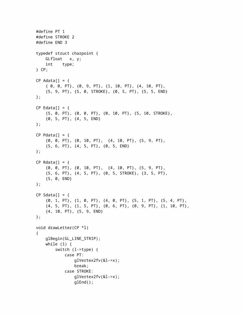
{    glViewport(0, 0, w, h);    glMatrixMode(GL_PROJECTION);    glLoadIdentity();    if (w <= h)         glOrtho (-1.5, 1.5, -1.5*(GLfloat)h/(GLfloat)w,             1.5*(GLfloat)h/(GLfloat)w, -10.0, 10.0);    else         glOrtho (-1.5*(GLfloat)w/(GLfloat)h,             1.5*(GLfloat)w/(GLfloat)h, -1.5, 1.5, -10.0, 10.0);    glMatrixMode(GL_MODELVIEW);    glLoadIdentity();}

int main(int argc, char** argv){    auxInitDisplayMode (AUX_SINGLE | AUX_RGBA | AUX_DEPTH);    auxInitPosition (0, 0, 500, 500);    auxInitWindow (argv[0]);    myinit();    auxMouseFunc(AUX_LEFTBUTTON, AUX_MOUSEDOWN,         changeRedDiffuse);    auxMouseFunc(AUX_MIDDLEBUTTON, AUX_MOUSEDOWN,         changeGreenDiffuse);    auxMouseFunc(AUX_RIGHTBUTTON, AUX_MOUSEDOWN,         changeBlueDiffuse);    auxReshapeFunc(myReshape);    auxMainLoop(display);}

Try This

Try This

Modify Example 6-3 :

Change the global ambient light in the scene. Hint: Alter the value of the GL_LIGHT_MODEL_AMBIENT parameter.  

Change the diffuse, ambient, and specular reflection parameters, the shininess exponent, and the emission color. Hint: Use the glMaterial*() command, but avoid making excessive calls.  

Use two-sided materials and add an arbitrary clipping plane (see "Additional Clipping Planes" ) so you can see the inside and outside of a row or column of spheres. Hint: Turn on two-sided lighting with GL_LIGHT_MODEL_TWO_SIDE, set the desired material properties, and add a clipping plane.  

Remove all the glMaterialfv() calls, and use the more efficient glColorMaterial() calls to achieve the same lighting.

The Mathematics of LightingAdvanced

This section presents the equations used by OpenGL to perform lighting calculations to determine colors when in RGBA mode. (You can find the corresponding calculations for color-index mode in "The Mathematics of Color-Index Mode Lighting." ) You don't need to read this section if you're willing to experiment to obtain the lighting conditions you want. Even after reading this section, you'll probably have to experiment, but you'll have a better idea of how the values of parameters affect a vertex's color. Remember that if lighting is not enabled, the color of a vertex is simply the current color; if it is enabled, the lighting computations described here are carried out in eye coordinates.

In the following equations, mathematical operations are performed separately on the R, G, and B components. Thus, for example, when three terms are shown as added together, the R values, the G values, and the B values for each term are separately added to form the final RGB color (R1+R2+R3, G1+G2+G3, B1+B2+B3). When three terms are multiplied, the calculation is (R1R2R3, G1G2G3, B1B2B3). (Remember that the final A or alpha component at a vertex is equal to the material's diffuse alpha value at that vertex.)

The color produced by lighting a vertex is computed as follows:

vertex color = the material emission at that vertex + the global ambient light scaled by the material's ambient property at that vertex + the ambient, diffuse, and specular contributions from all the light sources, properly attenuated

After lighting calculations are performed, the color values are clamped (in RGBA mode) to the range [0,1].

Note that OpenGL's lighting calculations don't take into account the possibility of one object blocking light from another, so shadows aren't automatically created. (See "Shadows" for a technique to create shadows.) Also keep in mind that with OpenGL, illuminated objects don't radiate light onto other objects.

Material Emission

The material emission term is the simplest. It's the RGB value assigned to the GL_EMISSION parameter.

Scaled Global Ambient Light

The second term is computed by multiplying the global ambient light (as defined by the GL_LIGHT_MODEL_AMBIENT parameter) by the material's ambient property (GL_AMBIENT's values as assigned with glMaterial*()):

ambientlight model * ambientmaterial

Each of the R, G, and B values for these two parameters are multiplied separately to compute the final RGB value for this term: (R1R2, G1G2, B1B2).

Contributions from Light Sources

Each light source may contribute to a vertex's color, and these contributions are added together. The equation for computing each light source's contribution is as follows:

contribution = attenuation factor * spotlight effect *

 (ambient term + diffuse term + specular term)

Attenuation Factor

The attenuation factor was described in "Position and Attenuation" :

attenuation factor =

where

d = distance between the light's position and the vertex

 kc = GL_CONSTANT_ATTENUATION

 kl = GL_LINEAR_ATTENUATION

 kq = GL_QUADRATIC_ATTENUATION

If the light is a directional one, the attenuation factor is 1.

Spotlight Effect

The spotlight effect evaluates to one of three possible values, depending on whether the light is actually a spotlight and whether the vertex lies inside or outside the cone of illumination produced by the spotlight:

1 if the light isn't a spotlight (GL_SPOT_CUTOFF is 180.0).  

0 if the light is a spotlight but the vertex lies outside the cone of illumination produced by the spotlight.  

(max {v x d, 0 } )GL_SPOT_EXPONENT where:

v = (vx, vy, vz) is the unit vector that points from the spotlight (GL_POSITION) to the vertex.

d = (dx, dy, dz) is the spotlight's direction (GL_SPOT_DIRECTION), assuming the light is a spotlight and the vertex lies inside the cone of illumination produced by the spotlight.

The dot product of the two vectors v and d varies as the cosine of the angle between them; hence, objects directly in line get maximum illumination, and objects off the axis have their illumination drop as the cosine of the angle.

To determine whether a particular vertex lies within the cone of illumination, OpenGL evaluates (max { v x d , 0 } ) where v and d are as defined above. If this value is less than the cosine of the spotlight's cutoff angle (GL_SPOT_CUTOFF), then the vertex lies outside the cone; otherwise, it's inside the cone.

Ambient Term

The ambient term is simply the ambient color of the light scaled by the ambient material property:

ambientlight *ambientmaterial

Diffuse Term

The diffuse term needs to take into account whether light falls directly on the vertex, the diffuse color of the light, and the diffuse material property:

(max { l ? n , 0 } ) * diffuselight * diffusematerial where:

l = (lx, ly, lz) is the unit vector that points from the vertex to the light position (GL_POSITION).

n = (nx, ny, nz) is the unit normal vector at the vertex.

Specular Term

The specular term also depends on whether light falls directly on the vertex. If l ? n is less than or equal to zero, there is no specular component at the vertex. (If it's less than zero, the light is on the wrong side of the surface.) If there's a specular component, it depends on the following:

The unit normal vector at the vertex (nx, ny, nz).  

The sum of the two unit vectors that point between (1) the vertex and the light position and (2) the vertex and the viewpoint (assuming that GL_LIGHT_MODEL_LOCAL_VIEWER is true; if it's not true, the vector (0, 0, 1) is used as the second vector in the sum). This vector sum is normalized (by dividing each component by the magnitude of the vector) to yield s = (sx, sy, sz).  

The specular exponent (GL_SHININESS).  

The specular color of the light (GL_SPECULARlight).  

The specular property of the material (GL_SPECULARmaterial).

Using these definitions, here's how OpenGL calculates the specular term:

(max { s x n , 0} )shininess * specularlight * specularmaterial

However, if 1 x n = 0, the specular term is 0.

Putting It All Together

Using the definitions of terms described in the preceding paragraphs, the following represents the entire lighting calculation in RGBA mode.

vertex color = emissionmaterial +

ambientlight model * ambientmaterial +

[ ambientlight *ambientmaterial +

(max { 1 x n , 0 } ) * diffuselight * diffusematerial +

(max {s x n ,0} )shininess * specularlight * specularmaterial ] i

Lighting in Color-Index ModeIn color-index mode, the parameters comprising RGBA values either have no effect or have a special interpretation. Since it's much harder to achieve certain effects in color-index mode, you should use RGBA whenever possible. In fact, the only light-source, lighting-model, or material parameters in an RGBA form that are used in color index mode are the light-source parameters GL_DIFFUSE and GL_SPECULAR and the material parameter GL_SHININESS. These parameters (dl and sl, respectively) are used to compute color-index diffuse and specular light intensities (dci and sci) as follows:

dci = 0.30 R(dl) + 0.59 G(dl) + 0.11 B(dl)

sci = 0.3 R(sl) + 0.59 G(sl) + 0.11 B(sl)

where R(x), G(x), and B(x) refer to the red, green, and blue components, respectively, of color x. The weighting values 0.30, 0.59, and 0.11 reflect the "perceptual" weights that red, green, and blue have for your eye - your eye is most sensitive to green and least sensitive to blue.

To specify material colors in color-index mode, use glMaterial*() with the special parameter GL_COLOR_INDEXES, as follows:

GLfloat mat_colormap[] = { 16.0, 47.0, 79.0 };glMaterialfv(GL_FRONT, GL_COLOR_INDEXES, mat_colormap);The three numbers supplied for GL_COLOR_INDEXES specify the color indices for the ambient, diffuse, and specular material colors, respectively. In other words, OpenGL regards the color associated with the first index (16.0 in this example) as the pure ambient color, with the second index (47.0) as the pure diffuse color, and with the third index (79.0) as the pure specular color. (By default, the ambient color index is 0.0, and the diffuse and specular color indices are both 1.0. Note that glColorMaterial() has no effect on color-index lighting.)

As it draws a scene, OpenGL uses colors associated with indices in between these numbers to shade objects in the scene. Therefore, you must build a color ramp between the indicated indices (in this example, between indices 16 and 47, and then between 47 and and 79). Often, the color ramp is built smoothly, but you might want to use other formulations to achieve different effects. Here's an example of a smooth color ramp that starts with a black ambient color and goes through a magenta diffuse color to a white specular color:

for (i = 0; i < 32; i++) {   auxSetOneColor (16 + i, 1.0 * (i/32.0), 0.0, 1.0 * (i/32.0));   auxSetOneColor (48 + i, 1.0, 1.0 * (i/32.0), 1.0);

}The auxiliary library command auxSetOneColor() takes four arguments. It associates the color index indicated by the first argument to the RGB triplet specified by the last three arguments. When i = 0, the color index 16 is assigned the RGB value (0.0, 0.0, 0.0), or black. The color ramp builds smoothly up to the diffuse material color at index 47 (when i = 31), which is assigned the pure magenta RGB value (1.0, 0.0, 1.0). The second loop builds the ramp between the magenta diffuse color and the white (1.0, 1.0, 1.0) specular color (index 79). Figure J-20 shows the result of using this color ramp with a single lighted sphere.

The Mathematics of Color-Index Mode Lighting

Advanced

As you might expect, since the allowable parameters are different for color-index mode than for RGBA mode, the calculations are different as well. Since there's no material emission and no ambient light, the only terms of interest from the RGBA equations are the diffuse and specular contributions from the light sources and the shininess. Even these need to be modified, however, as explained below.

Begin with the diffuse and specular terms from the RGBA equations. In the diffuse term, instead of diffuselight * diffusematerial , substitute dci as defined in the previous section for color-index mode. Similarly, in the specular term, instead of specularlight * specularmaterial , use sci as defined in the previous section. (Calculate the attenuation, spotlight effect, and all other components of these terms as before.) Call these modified diffuse and specular terms d and s, respectively. Now let s' = min{ s, 1 }, and then compute

c = am + d(1-s')(dm-am) + s'(sm-am)

where am, dm, and sm are the ambient, diffuse, and specular material indexes specified using GL_COLOR_INDEXES. The final color index is

c' = min { c, sm }

After lighting calculations are performed, the color-index values are converted to fixed-point (with an unspecified number of bits to the right of the binary point). Then the integer portion is masked (bitwise ANDed) with 2n-1, where n is the number of bits in a color in the color-index buffer.

[Previous chapter] [Next chapter]

See the About page for copyright, authoring and distribution information.