Limitations of Geiger-Mode Arrays for Flash LADAR Applications

George M. Williams, Jr.

Voxtel Inc., 15985 NW Schendel Ave. Ste. 200, Beaverton OR 97006, USA

ABSTRACT

It is shown through physics-based Monte Carlo simulations of avalanche photodiode (APD) LADAR receivers that under typical operating scenarios, Geiger-mode APD (GmAPD) flash LADAR receivers may often be ineffective. These results are corroborated by analysis of the signal photon detection efficiency and signal-to-noise ratio metrics. Due to their ability to detect only one pulse per laser shot, the target detection efficiency of GmAPD receivers, as measured by target signal events detected compared to those present at the receiver’s optical aperture, is shown to be highly particular and respond nonlinearly to the specific LADAR conditions including range, laser power, detector efficiency, and target occlusion, which causes the GmAPD target detection capabilities to vary unpredictably over standard mission conditions. In the detection of partially occluded targets, GmAPD LADAR receivers perform optimally within only a narrow operating window of range, detector efficiency, and laser power; outside this window performance degrades sharply. Operating at both short and long standoff ranges, GmAPD receivers most often cannot detect partially occluded targets, and with an increased number of detector dark noise events, e.g. resulting from exposure to ionizing radiation, the probability that a GmAPD device is armed and able to detect target signal returns approaches zero. Even when multiple pulses are accumulated or contrived operational scenarios are employed, and even in weak-signal scenarios, GmAPDs most often perform inefficiently in their detection of target signal events at the aperture. It is concluded that the inability of the GmAPD to detect target signal present at the receiver’s aperture may lead to a loss of operational capability, may have undesired implications for the equivalent optical aperture, laser power, and/or system complexity, and may incur other costs deleterious to operational efficacy.

Keywords: avalanche photodiode, APD, LADAR, laser radar, Geiger mode, photon counting

1. INTRODUCTION

Three-dimensional light detection and ranging (LADAR) imaging systems operate by spatially and temporally sampling the optical radiation presented to an array of detectors.1,2 A 3-D ladar arrangement combines predefined lateral scene information with range (depth) information; the resulting data set of angle-angle-range (AAR) polar coordinates and signal intensities allows 3-D images of the target to be constructed. Typically, range is found by time-of-flight measurements of one or more laser pulse returns reflected by the objects of a scene from a laser pulse used to interrogate the target, with the pulse returns recorded by the LADAR focal plane array (FPA) at nanosecond time scales. Lateral information is gathered through the use of a 2-D imaging scheme, either scanning or staring, for flash LADAR operation. The reflected intensity versus the time profile available at the LADAR aperture contains a convolution between the outgoing pulse shape and the surfaces located in the field of view (FOV) that is temporally sampled by the focal plane array (FPA). Due to the FPA’s difficulty in sampling at high rates, often only a limited number of time and intensity samples are collected by the sampling electronics. As in a traditional radar system, the location of surfaces in the scene can be ascertained from these pulse returns by using a matched-filter receiver that correlates the samples of the returned signal (and noise) with samples of a shape similar to the outgoing pulse. The target range can be determined from the peak sample of this filtered return pulse.2

Much research has been done to develop Geiger mode (Gm) avalanche photodiode (APD) arrays for single-pulse “flash LADAR” systems.3,4,5 Analysis of the signal photon detection efficiency (SPDE) and signal-to-noise ratio (SNR) metrics, both of which are functions of the detector dead time and the photon fluxes of signal, noise, and clutter, has shown that GmAPDs perform optimally only in the limit where the probability of detecting either a signal or noise electron during each range search interval (RSI) is much less than one. This is a result of the fact that GmAPD performance is greatly hampered by its ability to detect more than one photon per dead-time period.6 It is also for this reason that the performance of GmAPD LADAR degrades considerably when the target is partially obscured.4,7 When armed, GmAPDs fire upon the absorption of a single photon; thus, they respond more probably to objects in the

foreground of a scene, simply because the photons returned from foreground objects arrive at the optical aperture sooner than those from the target. Because a GmAPD’s dead time is long relative to the rate of incoming photons, later target photon arrivals at the GmAPD receiver’s optical aperture from the same pulse are not detected if an earlier photon event has been recorded.

The nonlinear temporal response of GmAPDs to noise and target signal events has a significant impact on their practical operation. The GmAPD LADAR target detection efficiency (i.e. the number of target photons detected relative to the number of target photons present at the optical aperture) is highly variable, and depends in unpredictable ways on the transmission and scattering properties of the scene (including the atmosphere and partially occluding media, such as vegetative canopies), the laser power, the target range, the pixel’s instantaneous field of view (IFOV), the reflective properties of the target, passive solar scattering from the scene, and the motion of the target with respect to the LADAR receiver. The probability that the detector is “armed” and available to detect the target photons present at the GmAPD LADAR receiver’s optical aperture cannot be predicted without prior knowledge of the scene and the target’s location. This renders the GmAPD LADAR receiver inefficient over most operational scenarios. Although accumulating the signal returns over multiple pulses may theoretically help in the detection of occluded targets, the GmAPD efficiency must be sufficiently low or the transmittance of the occluding media must be sufficiently high that there is some probability that the GmAPD pixel is armed and available to accumulate target photons when they arrive at the aperture. Furthermore, the process of signal accumulation is made difficult in the presence of platform motion and jitter, and pulse accumulation is also processing-intensive, causes laser-power problems, and increases platform size, weight, and power (SWAP). Furthermore, the binary response of the GmAPD does not record signal amplitude, causing all returns to be indistinguishable from single photons, regardless whether they actually represent single photon events or many more photons returned from potential targets.

To demonstrate the effects of GmAPD properties on flash LADAR operations, in this paper, we present a series of physics-based Monte Carlo simulations that were conducted to explore the effects of GmAPD noise and dead time on direct-detection LADAR systems. Slab models were constructed based on analytical approximations of foreground scattering media, including tree canopies, and scenes were modeled containing targets and real-world obscurants, with surface properties validated by bidirectional reflectance distribution function (BRDF) measurements.8 Ray tracing was used to develop spatially and temporally resolved photon flux densities at the receiver’s optical aperture. These were used to compare the performance of GmAPD and LmAPD LADAR receivers, and to investigate the effects of detector pulse detection efficiency (PDE) and dark count rate (DCR) that arise from different reset time (dead time) intervals and temporal sampling schemes, as well as conditions of receiver range, system laser power, FOV, target obscuration, and target reflectivity. We devote particular emphasis to the detection of targets under obscuring vegetative canopies; however, the lessons learned can be more generally applied to LADAR imaging through any transmitting and scattering medium.

It is shown that even with multiple pulse accumulation over staggered range search intervals (RSIs), and even under severely contrived operating scenarios, GmAPD array have very low target detection efficiency. It is also shown that GmAPD receivers cannot be expected to perform as well as LmAPD arrays in flash LADAR applications.9 This is anticipated because linear photon detection represents an upper bound on the performance of GmAPD detectors.6 And when using LmAPDs, light scattered from surrounding objects can provide additional target signal to the receiver’s aperture, which are most often not detected by GmAPD receivers.

2. BACKGROUND

Continual improvements in low-light-level and infrared imaging technologies have made them indispensible tools in surveillance, military operations, and homeland security. Such imagers operate, when immersed in the spatially and temporally varying photon flux of the battle space, which is composed of photons reflected, absorbed, and emitted from real-world objects, transform a portion of the photon flux present at the imager’s optical aperture and recording it as electronic signals that can then be displayed, transmitted, and processed to extract mission-critical information. In this process, the photon flux present at the imager’s optical aperture is transformed into a convenient coordinate space (e.g. an x–y space), with some introduction of noise and distortion. In area array imagers, the three spatial coordinates we are familiar with are recorded as two planar coordinates and the sequence of frames; i.e. the third axis represents the temporal sampling of the varying real-world photon cloud present at the optical aperture. (Additional dimensions of information about the incident photon energy, polarity or other measures might also be captured, depending on the detector.)

Object range information is valuable for most military operations, but is not easy to obtain from 2D imaging arrays. Over the last several decades, LADAR technologies have emerged, using eye-safe solid-state lasers with pulse powers of several kilowatts and pulse rates in the 104–105 Hz range to provide manned and unmanned military vehicles with previously unattainable abilities to understand scenes.10 While there are many diverse LADAR technologies, we concern ourselves in the present discussion with direct-detection flash LADAR systems. In these systems, a laser pulse is sent to interrogate a scene; its light is absorbed, reflected, and scattered off of objects in the world, and the return waveform, distorted in space and time by its interaction with the scene, is temporally registered by the pixels of an array. In this way a three-dimensional image of the scene can be recorded in polar coordinates (i.e., AAR coordinates). When the signal intensity is also recorded, a volume can be recorded in angle-angle-range-intensity (AARI) coordinates.

While high-resolution, low-noise, high-dynamic-range spatial and temporal sampling of the returning light will provide a more accurate representation of the scene, this goal is limited for LADAR (as for any imager) by practical system constraints and by the detector technologies that are available. Presently, most high-performance flash LADAR systems record the optical echo from the scene using a two-dimensional APD array, which is used to amplify the optical signal above the noise floor of the downstream electronics so that the amplitude and time of arrival of features in the temporally varying signal waveform can be recorded. In small-sized, low-spatial-resolution LADAR FPAs, it may be possible to record both time of flight and signal intensity for samples from the entire of the echoed photon stream, but in high-density, high-spatial-resolution LADAR FPAs, it may be possible to record the time of flight and signal intensity of only a few pulse returns, such as those features in the echoed waveform that might represent the leading edge, the peak amplitude response, the last return, or other pre-defined features of the pulse return. Often, this process is repeated a number of times, using the accumulated signal from multiple laser shots to improve the measurement’s SNR (signal to noise ratio). However, the ability to use multiple laser pulses to determine range information is limited by the relative motions of the sensor, the laser, and the objects in the scene, and by the system-level costs of increased laser power and repetition rate, the resulting thermal load, and the computational burden required to compensate for platform jitter and the relative motions of the platform and the target. These factors can have dramatic impacts on system utility, flexibility, and reliability.

Of the detector technologies being deployed for flash LADAR applications, GmAPD arrays have recently gained popularity11 for two main reasons, both of which are related to the large current that flows through the GmAPD when it is triggered by an optical pulse. First, GmAPDs are fairly simple to implement in a system. The read-out integrated circuit (ROIC) for these devices is generally a digital counter, which minimizes integrated circuit size.12,13 Second, GmAPDs are able to detect single-photon events. We note that in the visible band, GmAPD can be made using silicon,14,15 while in the near-infrared band, they are made using InGaAs, InGaAsP and InP.16

While GmAPDs’ strong current response makes them beneficial in some applications, the binary intensity response and the non-linear temporal response of this type of detector has serious drawbacks as well. Unlike an idealized LmAPD detector, a GmAPD does not respond to every primary electron from the target. First, the GmAPD is unable to record signal intensity information; only with the accumulation of multiple pulses can “grayscale” information be developed to inform calculations of a

Figure 2. Photon density measured through the canopy as a function of thescattering albedo. The larger signals detected at 2000 m correspond to the target. With high backscattering, the returns from the target approach 1 photon. Returns below “ground” represent multiple scattering events. Only the LmAPD return isshown, as the GmAPD cannot detect amplitude information — only the range of the top of the canopy.

Figure 1. Simple model used for the Monte Carlo simulation. A conical target2 m tall stands on the scene floor; a 10-m-thick scattering medium is located 5 m above the scene floor.

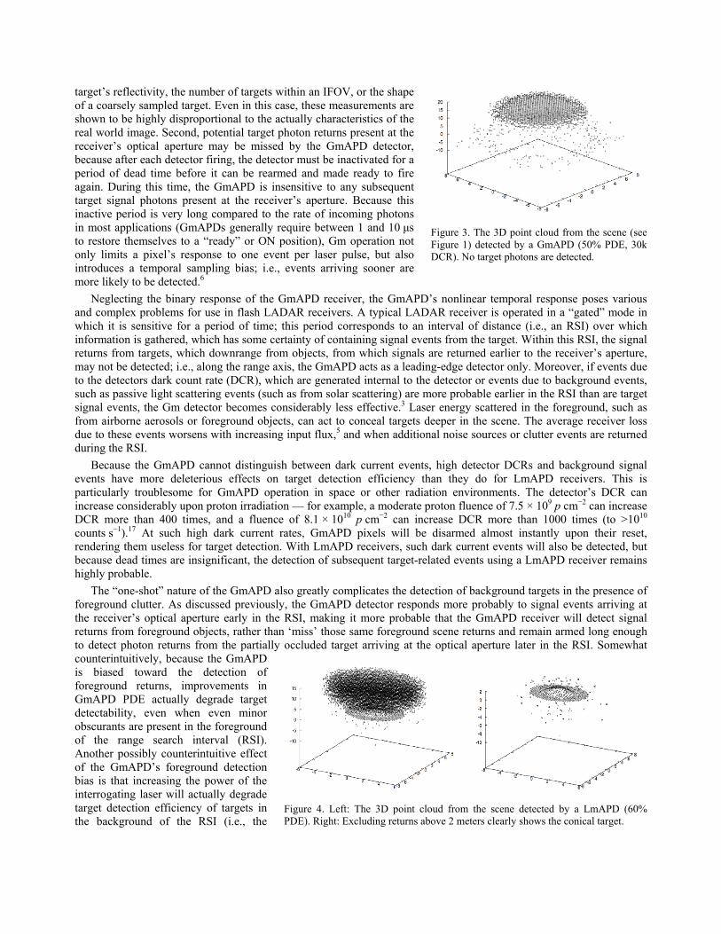
target’s reflectivity, the number of targets within an IFOV, or the shape of a coarsely sampled target. Even in this case, these measurements are shown to be highly disproportional to the actually characteristics of the real world image. Second, potential target photon returns present at the receiver’s optical aperture may be missed by the GmAPD detector, because after each detector firing, the detector must be inactivated for a period of dead time before it can be rearmed and made ready to fire again. During this time, the GmAPD is insensitive to any subsequent target signal photons present at the receiver’s aperture. Because this inactive period is very long compared to the rate of incoming photons in most applications (GmAPDs generally require between 1 and 10 μs to restore themselves to a “ready” or ON position), Gm operation not only limits a pixel’s response to one event per laser pulse, but also introduces a temporal sampling bias; i.e., events arriving sooner are more likely to be detected.6

Neglecting the binary response of the GmAPD receiver, the GmAPD’s nonlinear temporal response poses various and complex problems for use in flash LADAR receivers. A typical LADAR receiver is operated in a “gated” mode in which it is sensitive for a period of time; this period corresponds to an interval of distance (i.e., an RSI) over which information is gathered, which has some certainty of containing signal events from the target. Within this RSI, the signal returns from targets, which downrange from objects, from which signals are returned earlier to the receiver’s aperture, may not be detected; i.e., along the range axis, the GmAPD acts as a leading-edge detector only. Moreover, if events due to the detectors dark count rate (DCR), which are generated internal to the detector or events due to background events, such as passive light scattering events (such as from solar scattering) are more probable earlier in the RSI than are target signal events, the Gm detector becomes considerably less effective.3 Laser energy scattered in the foreground, such as from airborne aerosols or foreground objects, can act to conceal targets deeper in the scene. The average receiver loss due to these events worsens with increasing input flux,5 and when additional noise sources or clutter events are returned during the RSI.

Because the GmAPD cannot distinguish between dark current events, high detector DCRs and background signal events have more deleterious effects on target detection efficiency than they do for LmAPD receivers. This is particularly troublesome for GmAPD operation in space or other radiation environments. The detector’s DCR can increase considerably upon proton irradiation — for example, a moderate proton fluence of 7.5 × 109 p cm−2 can increase DCR more than 400 times, and a fluence of 8.1 × 1010 p cm−2 can increase DCR more than 1000 times (to >1010 counts s−1).17 At such high dark current rates, GmAPD pixels will be disarmed almost instantly upon their reset, rendering them useless for target detection. With LmAPD receivers, such dark current events will also be detected, but because dead times are insignificant, the detection of subsequent target-related events using a LmAPD receiver remains highly probable.

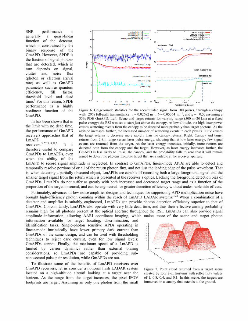
The “one-shot” nature of the GmAPD also greatly complicates the detection of background targets in the presence of foreground clutter. As discussed previously, the GmAPD detector responds more probably to signal events arriving at the receiver’s optical aperture early in the RSI, making it more probable that the GmAPD receiver will detect signal returns from foreground objects, rather than ‘miss’ those same foreground scene returns and remain armed long enough to detect photon returns from the partially occluded target arriving at the optical aperture later in the RSI. Somewhat counterintuitively, because the GmAPD is biased toward the detection of foreground returns, improvements in GmAPD PDE actually degrade target detectability, even when even minor obscurants are present in the foreground of the range search interval (RSI). Another possibly counterintuitive effect of the GmAPD’s foreground detection bias is that increasing the power of the interrogating laser will actually degrade target detection efficiency of targets in the background of the RSI (i.e., the

Figure 4. Left: The 3D point cloud from the scene detected by a LmAPD (60%PDE). Right: Excluding returns above 2 meters clearly shows the conical target.

Figure 3. The 3D point cloud from the scene (see Figure 1) detected by a GmAPD (50% PDE, 30k DCR). No target photons are detected.

increased light power serves instead to increase the probability of detection and range accuracy of foreground objects, such as the top of a tree canopy or a forward decoy object at the expense of partially occluded targets).18 These two effects are anticipated by previously developed theory.4–6,13,14,19,20

In a situation where clutter is not uniformly distributed but rather is more dense in the foreground of the RSI, such as in the example where a target is partially obscured in a forest canopy and where the LADAR receiver is at high altitude, there will be an extended canopy within each IFOV of the detector and the probability of a photon return from the top of the canopy will be high (due to more scattering events in the IFOV footprint); the target will therefore be masked by the foreground objects. As the range increases between the target and the LADAR receiver, GmAPD performance suffers; the number of foreground scattering elements in a pixel’s IFOV (for which detection is probable) decreases proportionally to the inverse square of the range; but less rapidly than does the signal from the target, which decreases much more rapidly, as the inverse fourth power of range. Thus, in a partially obscuring environment, increasing the target range significantly degrades the performance of the GmAPD receiver, as it becomes more probable that it will be disarmed due to intervening scattering objects. At long range, passive scattering events such as from the sun also become more probable. In general, it can be seen that GmAPD receivers work only when the PDE is reduced sufficiently so that foreground scene information available at the receiver is partially discarded. Only then, using multiple pulse accumulation with a ‘sliding’ RSI, is it possible to reconstruct a waveform that will make target detection possible.

In light of these drawbacks, the interest in GmAPD arrays for flash LADAR applications is somewhat curious. The intensity of photon flux from a scene generally contains valuable information about the scene, e.g. the reflective properties of the objects with which the photons of the pulse beam interacted, object range, and the spatial complexity of the objects in the pixel IFOV. While the GmAPDs provide a leading-edge (‘one shot’) temporal and a binary intensity record of scene and target information, which may be useful in rudimentary tasks, they essentially discard much of the information that a record of all of the target photons arriving at the optical aperture might provided. The disregard for a significant number of returned target photon events may, in fact, harm mission performance considerably. Clearly, it is desirable to obtain an undistorted representation of the photon cloud under low-light conditions; this goal is shared in the areas of intensified low-light-level imaging and infrared imaging. In light of the great effort devoted to preserving the target photons present at the optical aperture in other low light imaging modalities, allowing target photons present at the optical aperture of a GmAPD LADAR receiver to go undetected does not seemingly provide any obvious benefit. At long target acquisition range, there is a high energy cost for each photon returned. Considerable laser power is required to make a single photon return over the IFOV highly probable at long range. In systems whose detectors effectively discard a portion of the received spatial information, attaining a certain level of performance will incur a system cost of greater laser power or equivalent optical aperture. High-power lasers are perhaps the most demanding of platform components, and the use of larger collection optics increases system mass considerably; these costs increase the size, weight, and power (SWAP) of the system.

The receiver’s SNR and SPDE are useful LADAR FPA performance metrics. The SNR characterizes many of the sensor’s performance parameters, e.g. detection statistics and measurement errors. The SNR required for a specific mission depends on the precision goal required for that application; but for example, high-precision 3D measurements generally require an SNR on the order of 3 to yield a range error slightly better than the waveform’s range resolution, and a SNR of at least 100 is required to measure the target’s reflectance to within 10% of its mean. For a GmAPD, the

Figure 5. Monte Carlo simulation of notional canopy shown as a function of canopy transmittance (g = 0.1 and 0.5 shown here) and GmAPD efficiency. In both cases, high detection efficiencies diminish the probability of detecting the photons from the target that reach the optical aperture, because more efficient GmAPDs moreprobably detect the earlier signal returns from the top of the canopy. Only inefficientGmAPDs detect the target events in the background, because their probability of detecting the foreground objects is reduced. Even with optimal PDE, the targetdetection efficiency is very low.

SNR performance is generally a quasi-linear function of the detector, which is constrained by the binary response of the GmAPD. However, SPDE is the fraction of signal photons that are detected, which in turn depends on signal, clutter and noise flux (photon or electron arrival rate) as well as GmAPD parameters such as quantum efficiency, fill factor, threshold level and dead time.6 For this reason, SPDE performance is a highly nonlinear function of the GmAPD.

In has been shown that in the limit with no dead time, the performance of GmAPD receivers approaches that of LmAPD receivers.3−7,13,14,19,21 It is therefore useful to compare GmAPDs to LmAPDs, even when the ability of the LmAPD to record signal amplitude is neglected. In contrast to GmAPDs, linear-mode APDs are able to detect and temporally resolve portions of or all of the return photon flux, and not just the leading edge of the pulse waveform. That is, when detecting a partially obscured object, LmAPDs are capable of recording both a large foreground signal and the smaller target signal from the return which is presented at the receiver’s optics. Lacking the foreground detection bias of GmAPDs, LmAPDs do not suffer as greatly with both increased and decreased target range and as a function of the proportion of the target obscured, and can be engineered for greater detection efficiency without undesirable side effects.

Fortunately, advances in low-noise amplifier designs and techniques for suppressing APD multiplication noise have brought high-efficiency photon counting within the reach of LmAPD LADAR systems.7,22 When a combination of a detector and amplifier is suitably engineered, LmAPDs can provide photon detection efficiency superior to that of GmAPDs. Concomitantly, LmAPDs also operate with very little dead time, and thus their effective arming probability remains high for all photons present at the optical aperture throughout the RSI. LmAPDs can also provide signal amplitude information, allowing AARI coordinate imaging, which makes more of the scene and target photon information available for target locating, discrimination, and identification tasks. Single-photon sensitive APDs operating in linear-mode intrinsically have lower primary dark current than GmAPDs of the same design, and can be used with thresholding techniques to reject dark current, even for low signal levels; GmAPDs cannot. Finally, the maximum speed of a LmAPD is limited by carrier dynamics rather than external biasing considerations, so LmAPDs are capable of providing sub-nanosecond pulse pair resolution, while GmAPDs are not.

To illustrate some of the benefits of LmAPD receivers over GmAPD receivers, let us consider a notional flash LADAR system located on a high-altitude aircraft looking at a target near the horizon. As the range from the target increases, the pixel IFOV footprints are larger. Assuming an only one photon from the small

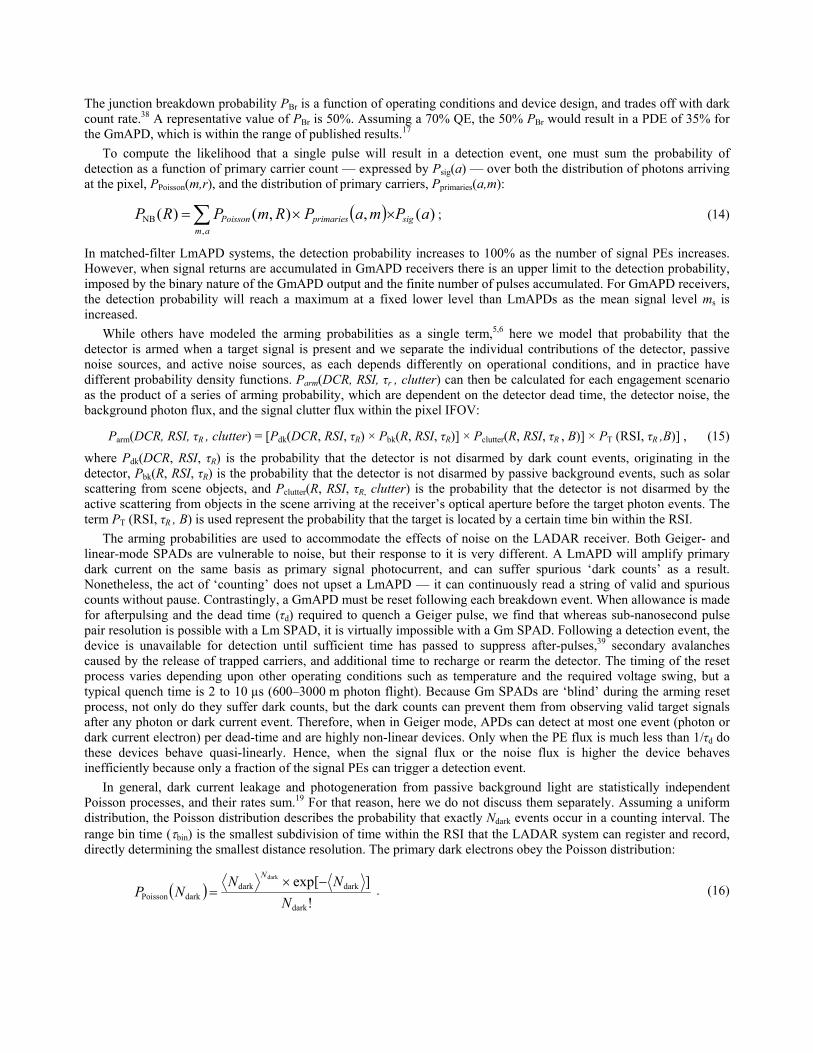
Figure 6. Geiger-mode statistics for the accumulated signal from 100 pulses, through a canopy with 20% full-path transmittance, a = 0.02682 m−1, b = 0.05364 m−1, and g = −0.5, assuming a 35% PDE GmAPD. Left: Scene and target returns for varying range (500 m–20 km) at a fixed pulse energy; the RSI was set to start just above the canopy. At low altitude, the high laser power causes scattering events from the canopy to be detected more probably than target photons. As the altitude increases further, the increased number of scattering events in each pixel’s IFOV causes the target returns to decrease more rapidly than the canopy returns. Right: Canopy and target returns from 2-km range versus laser pulse energy, showing that at low laser energy, few signal events are returned from the target. As the laser energy increases, initially, more returns are detected both from the canopy and the target. However, as laser energy increases further, theGmAPD is less likely to ‘miss’ the canopy, and the probability falls to zero that it will remainarmed to detect the photons from the target that are available at the receiver aperture.

Figure 7. Point cloud returned from a target scenecreated by four 2-m frustums with reflectivity valuesof 1, 0.8, 0.4, and 0.1. In this scene, the targets areimmersed in a canopy that extends to the ground.

sized target is probable, a GmAPD array and an LmAPD arrays, assuming an equal probability of photon detection in both of the arrays, are equally able to detect a single photon return from the target. However, if there is more than one target at that range or the target is embedded in clutter, the LmAPD array can receive a proportional signal that captures the information about the diverse objects in the scene, through the RSI. If more than one target is located at a specific range, the number of detection events within the LmAPD pixels will increase proportionally. The GmAPD does not share this ability.

Furthermore, in this scenario, if a small reflective airborne object (e.g. a decoy) is inserted along the line of sight in a monoaxial line with the laser beam, 1 km in front of the target, a GmAPD with a PDE approaching 100% will likely never detect signal returns from the target arriving at the receiver optics later in the RSI than those of the decoy, due to the detector’s dead time after the initial detection of the balloon. While the accumulation of multiple laser pulses and a time-varying RSI can be used to acquire the target signal, this approach comes at the expense of acquisition time, laser power, and computational costs. In contrast, the pixels of a LmAPD receiver can record the signal from many objects within a pixel’s IFOV. This scenario highlights the importance of recording all of the signal information available from LADAR returns in photon-starved environments.

There are, of course, limitations to the amount of information that can be collected and processed by an imager, but while some loss of fidelity can be expected in the operation of any practical system, there is no obvious value in using a detector that has the ability to record only the leading returns available in an RSI, often disregarding target signal returns, and which disregards target and scene signal intensity information.3

Figure 9. Photon detections from each of the target frustums (see Figure 7) for Geiger- and linear-mode detectors. Left: Target photon returns (per interrogating photon) for each of the frustums, shown as a function of the GmAPDs’ PDE. In the low-PDE regime, the differences in magnitude of returning photons recover some information on the differences in target reflectivity, but inhigher-PDE regimes, the GmAPD’s sampling bias degrades the receiver’s performance; efficient detection of early returns from thecanopy progressively blinds the receiver to later returns from the target. The optimal PDE is not constant among the differentconditions of target reflectivity. Right: LmAPD target photon returns (absolute) for each of the frustums. Because the LmAPDs are not biased toward early returns, the magnitude of target response recovers target reflectivity increasingly well in higher-PDE conditions; that is, improving PDE in an LmAPD does not entail any adverse effects.

Figure 8. A stacked bar chart showing the relative contribution of each frustum tothe total signal return, normalized to the return from the 100% reflective frustum.At low GmAPD PDE, the signal returns are proportional to the target reflectivity. At higher detector PDE values, the nonlinear response of the GmAPD causes thetarget detection efficiency to differ, until the number of target signal eventsdetected is approximately equal. At higher detector PDE, more scattering events from the canopy are detected, and here it is shown that the signal from the targetswith low reflectivity is larger than the higher reflectivity targets.

MONTE CARLO SIMULATIONS OF GMAPD AND LMAPD

ARRAYS

We used the Rochester Institute of Technology Digital Imaging and Remote Sensing Image Generation (DIRSIG) model to analyze the performance of GmAPD receivers and compare them to their and LmAPD counterparts. This section examines data that has been synthesized via direct simulation, but is compared below to SPDE and SNR metrics developed using theoretically derived probability distribution functions (PDFs). DIRSIG is an integrated collection of independent first-principles-based models that work in conjunction to produce radiance field images with high radiometric fidelity in the 0.3–30.0 μm region.23 DIRSIG’s rendering tool is built around a non-uniform subdivision ray tracer, which interacts with surfaces that are assigned material properties that include full bi-directional reflectance distribution functions (BRDFs). The ray tracer searches the scene geometry database to generate lists of surfaces along a given ray path, including opaque surfaces and obscuring transmissive surfaces (i.e. clouds, gas plumes, vegetation, etc.). Depending on the path geometry, the radiance computation can incorporate direct sky light or sunlight (for a clear path to the sky) or the reflected and emitted components from one or more surfaces along the path. Several sources of noise are extensively modeled, such as speckle from rough surfaces. The spectrally resolved radiometric calculations also account for atmospheric turbulence, including scintillation, beam effects, and image effects.24 The result is a spatially and temporally resolved photon cloud map at the input to the ladar optical aperture that can be used for a side-by-side demonstration of LmAPD and GmAPD detector technologies. This way, the detectors can be validated when operating in the direct simulation mode and compared to theoretically derived PDFs.

To test LmAPD and GmAPD LADAR receivers, we used DIRSIG to develop plate-type transmissive surfaces to model intervening atmosphere, camouflage, vegetation, etc. above targets. In our initial analysis, we first used a scene model containing a 10-m-thick simple model canopy model oriented 5 m from the ground, with a 2-m-high cone simulating the target (see Figure 1). In a canopy, the extinction of radiation depends on the area density distribution and normal orientation of the leaves; i.e., on the leaves’ slope distribution. Even very small contributions from large-angle scattering events can have a significant effect on the partial distribution of the reflected light.25 Some earlier canopy radiative transfer formulations have assumed that the canopy has an isotropic scattering phase function;26 however, theory and experiments have shown that the canopy phase function is rotationally variant. The phase function depends not only on the scattering angle, but also on the incident and outgoing directions.27

The properties of the vegetative canopy here were simulated by imparting a simple Henyey-Greenstein (HG) scattering phase function,28 which has proven to be useful in approximating the angular scattering dependence of single scattering events, and has been used previously to simulate tree canopies.29 The HG function is an approximation to the real phase function. The scattering asymmetry parameter controls the shape of the phase function, with g = 0 for isotropic scattering, positive g for forward throwing, and negative g for a phase function dominated by back-scattering. As a result, this formulation still can be used to study the angular dependence of reflectance from a canopy for LADAR system design.

The vegetative density of the canopy was modeled using plates of varying transmittance (0 to 100%) and scattering albedo (+0.9 to −0.9). The average returns measured from dot clouds synthesized via direct simulation of the flat-plate targets are shown in Figure 2 for a LADAR scene interrogated at a range of 2 km by a 1-mJ laser with an 8-mrad half angle divergence. The data recorded by the LmAPD LADAR sensor module was used to plot the returns from single laser pulses (2 ns FWHM). The forward component of the scattering angle strongly influences the photon density; with more photons scattered forward, more returns arrive from objects deeper in the canopy. With more backscattering, the

Figure 10. Visualization of LmAPD and GmAPD returns. Left: Unprocessed point cloud of a scene as detected by the LmAPD receiver. Note the significant number of points below the targets, representing photons scattered from the scene and reflected from the target Right: the GmAPD response also shows the targets, but the distribution of returns about the ground provide less range precision than the LmAPD, and the ‘one-shot’ pixels do not efficiently detect the photons scattered from scene objects to the target, which arrive at the optical aperture later in the pulse stream.

photon flux at the target is decreased to single-photon levels. While it is possible to use this same approach to model scattering aerosols in the atmosphere, the atmospheric effects and the interaction of the atmosphere and the canopy were excluded from these simulations for simplicity.

Shown in Figure 3 and Figure 4 are the point clouds showing the target scene (with full-path transmittance 20% and scattering albedo g = 0.9) as recorded by a GmAPD receiver (PDE = 50%) and an LmAPD receiver (PDE = 60%). Due to its one-shot, leading-edge temporal sampling, the GmAPD never detects the target, whereas the target is clearly present in the LmAPD returns registered below 2 m in the point cloud.

To test the influence of canopy transmission on the operational performance of GmAPD receivers, the detected scene and target signal events were temporally registered and recorded as heights, as a function of GmAPD efficiency. Shown in Figure 5 are the cases for a canopy with scattering albedo characterized by the HG phase functions with g = 0.1 (mostly opaque) and 0.5 (dappled ground). In the case of the low-transmittance canopy (g = 0.1), the GmAPD LADAR receiver does not accurately detect the height of the canopy when PDE is less than 0.003; both the mean and median of the pulse returns are well below the top of the canopy, confirming the poor range accuracy. The lack of range precision in lower-PDE conditions is a simple consequence of the fact that the leading-edge photons returning from the top of the canopy are not consistently detected by the GmAPD, and that some of the photons detected have returned from elastic scattering events later in the RSI. The record of minimum canopy height returns, recorded below ground level, signifies that the poor PDE of the receiver allows for sufficient foreground scene signal events to go undetected such that detection of target signal events becomes more probable. In such low-PDE cases, some GmAPD pixels remain armed long enough to detect photons later in the pulse return.

As GmAPD efficiency increases, the GmAPD array is able to detect the top of the canopy with increasing accuracy (note that the maximum height values slightly above the actual 15-m canopy arise from the Gaussian-modeled temporal shape of the laser pulse). The variability of the canopy height measurement can be seen to continue to diminish as the detector PDE improves. However, as the PDE of the GmAPD continues to increase, discernable returns from the target increasingly are not detected, because the target signals present at the optical aperture are not detected by the GmAPD detector when it has been disarmed by signal from the canopy. It should be noted that in this example, an 40-m RSI was used so that the GmAPD was armed just before the returns from the canopy arrives, and so the effects of atmospheric scattering and the detector’s DCR (here, 30k counts/s) could be neglected. Solar and lunar contributions were also neglected; their inclusion would degrade GmAPD performance relative to the examples shown.

For a full-path canopy transmittance of 0.5, it can be seen that a sufficient number of photons are transmitted through the canopy (through ‘hot spots’ unobscured by leaves) to allow the target to be

Figure 12. Point cloud representations for a 16 × 16-element array with the same FOV and range (1250 m) as the figures above. As the IFOV footprint is increased (simulating longer range), the LmAPD (left) records significantly more photons fromthe target at long range. The GmAPD (right) generates only 256 points (one per pixel), with a larger portion originating from objects earlier in the RSI. The larger IFOV footprint causes the distribution of GmAPD returns to be originated at sceneobjects closer to the receiver. Only unobscured target returns were recorded by the GmAPD. A 35% GmAPD and a 65% LmAPD PDE were used, and the GmAPD DCRwas set to 30,000 counts/s, which for the 40-m RSI did not influence the results.

Figure 11. A 72 × 72 µm pixel, 128 × 128-element FPA at 1250 m with the same FOV as shown in Figure 10. (LEFT): The point cloud generated by the LmAPD array, showing a large number of photons directly scattered from the target as well as those scattered from the scene and returned from the target. Right: The GmAPD registers at most one return per pixel.

detected if GmAPD PDE is below 0.001. In these low-PDE conditions, the GmAPD’s range accuracy is diminished, as reflected in the recorded canopy height measurements. Again, as the PDE of the GmAPD improves, the range accuracy increases but the probability of detecting the target decreases; the pixel is more likely to be disarmed by canopy signal events arriving at the optical aperture, which masks the later target signal returns.

To further illustrate the variable effect of operational, receiver, and scene characteristics on the performance of GmAPD LADAR receivers, signal returns were recorded for a GmAPD receiver with fixed FOV and fixed laser power, as a function of altitude (target range). In this case, the returns from 100 laser shots were accumulated. At low altitude, the laser power is sufficiently high that the strong signal returns from the top of the canopy serve to cause the GmAPD to be disarmed before later target signal events arrive at the optical aperture (Figure 6, left). Here, a highly transmissive canopy (full-path transmittance = 0.20) was used to allow a high probability of target signal events from being recorded. At longer ranges, the signal returned from the canopy is reduced at a rate which can be predicted by theory to be proportional to the range squared, and the signal returning from the canopy similarly reduces as proportional to the range squared until it is unresolved and the signal reduces proportionally to the fourth power of the range. As range increases, the number of scattering events within each pixel’s IFOC footprint increases, and the probability that the GmAPD detector is armed for detecting target signals arriving at the optical aperture from later in the RSI is diminished.

Similar effects are observed with varying laser energy (Figure 6, right). However, here, rather than the canopy signal increasing due to the increased number of scattering events in each pixel’s IFOV footprint, the stronger canopy return is simply a result of the increased number of signal events that is a result of the increased laser pulse energy. It can be seen in the plots, when sufficiently low laser pulse energies are used, there is a probability that photons present at the aperture from returns off of the canopy go undetected by the GmAPD, such that the detector is armed for detection when the target signal photons are present at the aperture. While these target returns have the same probability as going undetected as those from the canopy, due to the detector’s low PDE, there remains some probability that a signal can be detected and accumulated over multiple laser shots. At higher laser pulse energies the target signal begins to approximate the height of the target. However, as the laser pulse energy is further increases, the number of photon events from the canopy increases, and the probability of the GmAPD being armed for detection of target signal events is reduced. The curves of Figure 5 and Figure 6 illustrate an important characteristic of the GmAPD LADAR receivers. In these examples, one of more of the platform variables was held constant, for the purposes of illustration; however, in real-world situations the laser power at the scene, the IFOV footprint, and the transmittance of the canopy all vary with changing target range (altitude). Because of the interactions of these non-linear variables, the operating range of GmAPD receivers is quite small, and to achieve a target signal, in most operational scenarios it is necessary to have a priori knowledge of the scene and the target so that the receiver’s operational parameters can be optimized to make target detection more probable. It can also be seen in these plots, that when the target detection becomes probable, the GmAPD receiver is most often operating every inefficiently (as indicated by a low number of target signal events recorded versus the number of target signal events present at the aperture).

To further examine the operation of GmAPD receivers, a series of frustums were modeled, each within the FOV of a 64 × 64-element subsection of a 128 × 128-element APD array (see Figure 7). In contrast to the example above, here 2-m-high frustums were embedded within a canopy model. An absorption coefficient of a = 0.0187 was used with a scattering coefficient of b = 0.0187 and an HG scattering phase function with g = 0.5. In these examples, a 2-ns, 1-mJ laser pulse with an 8-mrad 1/e2 divergence half angle was used to interrogate the frustum targets embedded in the 40-m-thick medium. The number of photons detected compared to the number sent (the photon efficiency) was plotted for a variety of PDE values. As shown in Figure 9 (left), which plots the number of target signal events recorded as a function of the laser photons sent, plotted against the GmAPD PDE, for low GmAPD efficiencies, the number of photons reflected from the target is approximately proportional to the number of photons sent. However, as the GmAPD detector

Figure 13. The waveforms recorded by random pixelsselected from the LmAPD FPA, showing that the largeIFOV footprint increases the photon density from thecanopy as well as the ground. The waveforms show that thetarget signal is preserved, and also show a significantnumber of returns detected by the LmAPD receiver due tophotons scattered from the scene to the target. These eventsare clearly apparent as returns with negative height values.

efficiency increases (e.g. above PDE = 0.02), the non-linear temporal response of the GmAPD begins to impact performance, and the detected signal returns are no longer proportional to the target’s reflectivity. As the APD detectors detecting the higher-reflectivity targets saturate, the difference in photon returns measured from each of the reflective surfaces (with r = 1.0, 0.8, 0.4, and 0.1) decreases. At GmAPD detector efficiencies above 0.06, the probability of photon events from the canopy present at the optical aperture earlier in the RSI, causes the detector to become increasingly disarmed when target signals arriving later in the RSI arrive at the receiver’s aperture causing the Gm LADAR receiver to be blind to the target. In contrast, the photon events detected by a LmAPD (see Figure 9, right) increase as the LmAPD receiver PDE (throughput) increases. The LmAPD also demonstrates the ability to record target signal events proportionally to the target’s reflectivity. The accuracy of the target reflectivity increases as the LmAPD efficiency increases. In this example the LmAPD was modeled with a 65% PDE, a 1-ns temporal response, and a 2-ns dead time.

To examine the nonlinear response of the GmAPD to the reflective properties of the target, the signals returned from each frustum were recorded. Shown in Figure 8 are stacked bar charts showing the relative target photons detected, normalized to the response of the return from the 100% reflectivity frustum. Compared to the proportional signals recorded by the LmAPD example shown in Figure 9 (right), the response of the GmAPD is non-linear with respect to target reflectivity over all GmAPD efficiency values, and at high detector PDE values, the signal from low reflective targets exceeds that of the 100% reflective target.

Next, simulated scenes were used to illustrate the above recorded LADAR receiver properties in simulated real-world environments. Using targets and tree models made available by RIT, each developed using material properties modeled from BRDF measurements, a model scene was generated and imported into DIRSIG. Figure 10 shows the unprocessed point clouds representing the returns received from the scene from a 80-mJ pulse originating at a range of 1.25 km, received by the receiver’s 5-cm optical aperture, and focused onto a 256 × 256-element, 36 × 36-μm pixel FPA. An RSI beginning just above the treeline was used to mitigate any of the deleterious effects of dark current events. In this case, the GmAPD array, shown left in the figure, shown a scene composed of various height trees, below which are a SCUD launcher (partially below maple trees) a truck (below a hickory tree), a camouflaged HUMVEE, and a mostly canopy occlude HUMVEE. For this simulation, the GmAPD FPA detected 61,897 signal events, roughly one for each of the 2562 pixels in the array. The LmAPD array (shown in the left half of Figure 10) detected 80,010 signal returns, with 2,210 pixels detecting 2 pulse returns, 431 pixels detecting 3 returns, and 120 pixels detecting more than 3 returns. In the case of the LmAPD receiver, the average magnitude (intensity) of the LmAPD returns, across all pixels, was 41,500 DN, with DN, the digital number, reflecting the number of photon events detected in during that time event. When averaged across all pixel returns, the simple, unweighted average scene height from the LmAPD returns was calculated to be 12.57 ± 15.48 m, while for the GmAPD receiver, the average scene height was calculated to be 14.50 ± 15 m. The differences in the average scene height between the two types of detectors is a result of the GmAPD preferably detecting pulse returns from the objects in the foreground, while the LmAPD is sensitive to returns from throughout the scene. Note, also, that the 3D point cloud generated from the returns of the LmAPD receiver, include contributions from events attributed to heights below ground (negative height). This is simply a result of the LmAPDs ability to be armed for the arrival of photons, which are scattered from objects on the scene, and reflecting off of the target, such that their path lengths causes them to arrive at the scene later than signal events reflected from the ground. As the path length of these photons is longer, they have a later time of arrival than do photons with a shorter path length. It is shown that even for this simple scene a significant portion of the target returns can be attributed to multiple path scattering. While it is difficult to see in the images, it is noticeable, upon examination, that the GmAPD returns attributed to the ground have a relatively wide variance about the mean, which is a result of the poor GmAPD range accuracy compared to LmAPD receivers.

To detect the effects of target range, each receiver was simulated at ranges from 500 to 10,000 km. It was shown, as predicted by the slab models described above, that at longer range, foreground scatters reduced the ability of GmAPDs to detect target returns. This was verified by testing the receivers’ performance at a fixed range, FOV, and laser power, and by increasing the pixel size, so that the footprint of each pixel on the scene was increased proportionally.

Illustrated in Figure 11 is an unprocessed 3D point cloud generated by a receiver, temporally and spatially sampling the same photon flux as the example shown in Figure 10. In this case, like the last a receiver at a 1250 m altitude, with a fixed FOV was used to laterally and temporally record the scene. In this case the pixels were scaled from 36 × 36 μm to 36 × 36 μm (128 × 128 spatial elements). The results illustrate the effects of increased pixel IFOV footprint (GSD). As the number of GmAPD FPA elements decreases, the number of points in the 3D image increases proportionally, and in this case, the number of signal events from the target decreases more than those from other objects in the scene. This is

simply due to the larger number of foreground scattering events within each pixel’s IFOV. In the case of the LmAPD (Figure 11 left), the larger number of foreground scattering events is shown in the signal intensity (not shown here). The ability to record the return waveform is only limited by the LmAPD’s dead time (which was modeled in here to be 2 ns). As before, the LmAPD receiver shown a significant number of target events resulting from signal scattered from the scene (indicated by ‘below ground’ signal events underneath each target). The GmAPD receiver does not efficiently capture scattered target signal events.

Shown in Figure 12 are the 3D point clouds generate by the receiver modeled above, in this case with a 16 × 16-element FPA composed of 576 × 576-μm pixels. When the LmAPD receiver with a 65% PDE and a 2-ns dead time was used to sample the photon cloud present at the optical aperture, there were 5,085 signal returns — about 4750 more than the GmAPD array detected (Figure 12). In the case of the LmAPD receiver, as many as 25 pulses returns were recorded within each pixel. Due to the increased number of scattering events within each pixel IFOV, the amplitude of each LmAPD pulse response was, on average, 593,000 DN. Waveforms developed from event-driven temporal sampling at random pixels of the LmAPD receiver are shown in Figure 13. It can be seen in these waveforms that returns from both the scene and the targets are present in the waveforms, which makes the post-processing recovery of the target signature likely.

The above Monte Carlo simulations used static scene models, and in all of these simulations a series of single laser shot or the accumulation of ten or a hundred laser pulses was used. When implemented in a matched-filter LADAR, the photoelectrons (PEs) from multiple laser pulses are often accumulated; Neyman-Pearson detection algorithms can be applied to the accumulated signals in each independent range gate defined by the length of the matched-filter integration period. In applications considering moving targets, a “shift and sum” approach can also be used in which a series of digitized laser pulse returns is “stacked” into a large matrix. In an alternate “numerically shift and histogram” approach, only the time of an event (and amplitude of this time event as an option) is stored in the computer for each laser pulse return;30 all zeros are ignored. The event times for each return pulse are then numerically shifted by arbitrary time increments in sequence, and a time histogram is computed for each shift. The histogram with the maximum time bin value is declared a “detection” if the value exceeds a threshold, and the corresponding numerical shift estimates the range rate as well.

4. ANALYSIS OF RESULTS

The Monte Carlo results can be explained using LADAR receiver operating characteristics (ROCs) developed from the receiver’s probability density functions.4,6,13,14,20,20,31 The total spatially and temporally varying optical power incident on an APD receiver consists of four components:

S(tk, xi, yj) = Ss(tk, xi, yj) + Sc(tk, xi, yj) + Sbg(tk, xi, yj) + Sd(tk, xi, yj) , (1)

where Ss(tk,xi,yj) is the signal power and Sc(tk,xi,yj) is the power from clutter or target obscurants, both of which depend on transmitter power. Sbg(tk,xi,yj) is passive background light power, and Sd(tk,xi,yj) is dark-current-equivalent optical power, neither of which depend on the transmitted laser energy. This total light power is transduced into a proportional primary (pre-gain) photocurrent; the observed number of primary carriers is denoted as (tk,xi,yj):

(tk,xi,yj) = s(tk,xi,yj)+ bg(tk,xi,yj)+ c(tk,xi,yj)+ n(tk,xi,yj) = ηqe[Ss(tk,xi,yj) + Sc (tk,xi,yj)+ Sbg (tk,xi,yj)+ Sd(tk,xi,yj)]/hν , (2)

where h is Planck’s constant, ν is the LADAR’s optical frequency, and the product hν is the photon energy.

Each FPA’s FOV is determined by the physical size of the array and the optical system design. For target ranges where the ground sample distance (GSD) of each pixel’s IFOV footprint is larger than the target, the strength of the reflected return from the target depends upon the cross sectional area presented by the target (Atgt). At ranges for which the target is larger than the pixel’s IFOV footprint, the strength of the reflected return depends upon the area of the IFOV footprint on the target (AIFOV). It is assumed here that only one pixel in the LADAR detector array is being analyzed. Thus, the spatial indexing coordinates (xi, yi) are omitted in further analysis. In the limiting case of a small on-axis target in the far field, the number of photons detected at the aperture of the receiver is32

),(4

π)(

2

2

systx

s RλTR

DRρξη

hc

Eλψ , (3)

where Etx is the pulse energy, ηsys is the system efficiency factor, accounting for losses within the transmitting and receiving optics; ρ is the reflectivity of the target, ξ(R) is a geometric correction factor; R is the range; T(λ,R) is the full-path transmittance, and D is the diameter of the receiving optics. The factor ξ(R) is determined by the geometric considerations of the receiver optics and the overlap between the transmitted laser beam and the field of view of the receiver; for an infinite diffuse target, ξ(R) = 1; for the limiting case of a small on-axis target in the far field, ξ(R) = 2π (At/Ab), where At = πD2/4 is the area of the on-axis target and Ab = π(λR/πw0)

2 is the beam area at the target plane (with beam waist w0). Truncation and telescope obscuration distort the beam; the resulting non-Gaussian far-field effects can also be modeled.33 Note that for typical operational ranges, the range R and the axial distance are nearly equal, and the signal power varies as R−4.

In a direct-detection ladar system, the signal received from the target is the integrated irradiance at the receiver aperture. Goodman34,35 notes that the statistics of the integrated irradiance are well approximated by a gamma-distributed random variable where the number of degrees of freedom in the gamma distribution is the number of spatial correlation (speckle) cells at the aperture times the number of signals averaged. Coherent light reflected from a diffuse surface undergoes laser speckle; the integrated irradiance of this light has a negative binomial distribution. The negative binomial distribution is parameterized by the mean number of photoelectrons, m, and a diversity parameter MR that represents the mean number of correlation cells at range R:36

RM

R

R

m

R

R

R

R

M

m

m

M

Mm

MmRmP

11

Γ!

Γ),(NB

, (4)

where

0

1 )exp()(Γ ttdtz z is the gamma function. For MR = 1, the negative binomial distribution reduces to the

Bose-Einstein distribution. If the mean number of photoelectrons is held constant and the diversity increases, the distribution converges to the Poisson distribution. The negative binomial distribution also approaches the Poisson distribution as the mean number of photoelectrons approaches zero. If we accordingly assume that the signal photon statistics are Poisson-distributed, the probability of m photons arriving at the pixel is

!

exp),(Poisson

m

mmRmP R

m

R

. (5)

The efficiency with which the detector transduces the signal photons, i.e., its signal photon detection efficiency (SPDE) is the ratio of the signal detection probability to the mean number of signal photons incident on the APD. SPDE can be calculated as the product of the detectors signal detection efficiency and its arming probability Parm(DCR, RSI, τR , clutter), which is a function of the detector’s dark count rate (DCR), the size of the RSI (range search interval), the duration of the range bin τr, and a parameter to account for clutter in the scene (clutter). With the exception of the arming probabilities, the SPDE of a GmAPD array will be identical to that of a linear photon counter when operated in conditions of weak signal and weak noise; in this regime, the GmAPD should behave quasi-linearly.6 The SPDE can be calculated as5

SPDE = PDE(R) × Parm(DCR, RSI, τR , clutter) , (6)

where PDE(R) is a function of the detector’s quantum efficiency (ηq) and its ability to generate sufficient signal from these primary photocarriers such that a threshold level is exceeded, and Parm(DCR, RSI, τR , clutter) is the probability that the detector is armed for the target photons present at the aperture throughout the RSI. If the primary quantum efficiency of an lmAPD’s absorber is ηq, then the probability of creating a primary photoelectrons from m photons is:

!!)(

!)1(),(primaries

aam

mηηmaP am

qaq

, (7)

where m ≥ a, and the average number of electrons generated is simply RqR

mηa .

A LmAPD can detect a weak signal if its internal multiplication gain is high enough to boost the signal photocurrent above the noise floor of the receiver’s amplifier. The output level of a linear-mode APD photoreceiver can be treated as the sum of the APD’s output and the input-referred noise of the transimpedance amplifier (TIA). The two fluctuating quantities are uncorrelated, so the probability density function that characterizes the receiver level at the output of the

APD (input of the TIA) is the convolution of the output pulse height distribution (PHD) of the APD (PHDAPD) with the input-referred PHD of the TIA noise (PHDTIA):

TIAAPDreceiver PHDPHDPHD . (8)

The TIA’s PHD is generally taken to be Gaussian, characterized by a certain RMS input-referred current noise if it is a resistive feedback TIA (RTIA), or an RMS input-referred charge noise if it is a capacitive-feedback TIA (CTIA). The normalized Gaussian distribution is:

)var(2

)(exp

)var(2

1)(

2

n

nn

nnPHDTIA

. (9)

The APD’s PHD depends upon what type of APD it is. Successive impact-ionization events in the multipliers of most APDs are uncorrelated, and the lowest excess noise factor which can be achieved at any appreciable gain is F = 2. Silicon and InGaAs APDs fall into this category. The McIntyre PHD, parameterized in terms of the number of primary input carriers (a = 1 for photon counting), the average avalanche gain M, and the ratio of the impact-ionization rate of holes to that for electrons (k) is:

ank

nka

APD M

Mk

M

Mk

ak

nkann

k

na

nPHD

1111

11

!

11 1

, (10)

where Γ, the gamma function, is defined as

0

1 exp ttdtz z .

It should be noted that the discrete PHDs for APDs represent total output of the multiplication process in units of the elementary charge, without reference to the time-sequencing of the output. The avalanche process of real-world APDs occurs over a finite period of time, and takes longer to complete for higher-gain avalanche chains. This means that PDE calculations based upon these PHDs are more accurate for charge-integrating receivers based upon CTIAs than for current-sensing receivers based upon RTIAs. In particular, single photon detection with an RTIA receiver is based upon the height of the current pulse emitted by the APD. Junction current is proportional to the instantaneous population of charge carriers in the junction, according to Ramo’s theorem.37 This means the statistical distribution of the current peak height will match the particle PHD only if the avalanche process completes before any of the secondary carriers leave the junction. In many APDs this is not the case at high gain, and numerical Monte Carlo methods are required to simulate the current peak distribution, taking the junction transit time and temporal evolution of the avalanche process into account.

PDE depends upon the receiver’s count threshold, which is selected to reject noise counts from the amplifier. The PHDs are normalized, so the probability that either the TIA noise, or the convolution of the APD’s output with the TIA noise, exceed a given threshold level is found by summing the relevant PHD:

th

)()( thni

nPHDnnP . (11)

It is often more computationally efficient to sum the PHD from 1 to nth, and to subtract the sum from unity. This is the chance that the pulse will not be detected, this results in the following probability of signal detection

thn

i

nPHDaP1

Lm sig, )(1)( . (12)

The expression for Geiger SPADs is considerably simpler. At any given operating point above the breakdown voltage, the detector is characterized by the parameter PBr, which gives the probability that a single primary photocarrier injected into the multiplication layer of the APD will trigger avalanche breakdown. Consequently, the probability of detecting a primary carriers is simply one minus the probability that none of the carriers triggers breakdown, PBr:

aPaP )1(1)( BrGmsig, . (13)

The junction breakdown probability PBr is a function of operating conditions and device design, and trades off with dark count rate.38 A representative value of PBr is 50%. Assuming a 70% QE, the 50% PBr would result in a PDE of 35% for the GmAPD, which is within the range of published results.17

To compute the likelihood that a single pulse will result in a detection event, one must sum the probability of detection as a function of primary carrier count — expressed by Psig(a) — over both the distribution of photons arriving at the pixel, PPoisson(m,r), and the distribution of primary carriers, Pprimaries(a,m):

)(,),()(,

NB aPmaPRmPRP sigam

primariesPoisson ; (14)

In matched-filter LmAPD systems, the detection probability increases to 100% as the number of signal PEs increases. However, when signal returns are accumulated in GmAPD receivers there is an upper limit to the detection probability, imposed by the binary nature of the GmAPD output and the finite number of pulses accumulated. For GmAPD receivers, the detection probability will reach a maximum at a fixed lower level than LmAPDs as the mean signal level ms is increased.

While others have modeled the arming probabilities as a single term,5,6 here we model that probability that the detector is armed when a target signal is present and we separate the individual contributions of the detector, passive noise sources, and active noise sources, as each depends differently on operational conditions, and in practice have different probability density functions. Parm(DCR, RSI, τr , clutter) can then be calculated for each engagement scenario as the product of a series of arming probability, which are dependent on the detector dead time, the detector noise, the background photon flux, and the signal clutter flux within the pixel IFOV:

Parm(DCR, RSI, τR , clutter) = [Pdk(DCR, RSI, τR) × Pbk(R, RSI, τR)] × Pclutter(R, RSI, τR , B)] × PT (RSI, τR ,B)] , (15)

where Pdk(DCR, RSI, τR) is the probability that the detector is not disarmed by dark count events, originating in the detector, Pbk(R, RSI, τR) is the probability that the detector is not disarmed by passive background events, such as solar scattering from scene objects, and Pclutter(R, RSI, τR, clutter) is the probability that the detector is not disarmed by the active scattering from objects in the scene arriving at the receiver’s optical aperture before the target photon events. The term PT (RSI, τR , B) is used represent the probability that the target is located by a certain time bin within the RSI.

The arming probabilities are used to accommodate the effects of noise on the LADAR receiver. Both Geiger- and linear-mode SPADs are vulnerable to noise, but their response to it is very different. A LmAPD will amplify primary dark current on the same basis as primary signal photocurrent, and can suffer spurious ‘dark counts’ as a result. Nonetheless, the act of ‘counting’ does not upset a LmAPD — it can continuously read a string of valid and spurious counts without pause. Contrastingly, a GmAPD must be reset following each breakdown event. When allowance is made for afterpulsing and the dead time (τd) required to quench a Geiger pulse, we find that whereas sub-nanosecond pulse pair resolution is possible with a Lm SPAD, it is virtually impossible with a Gm SPAD. Following a detection event, the device is unavailable for detection until sufficient time has passed to suppress after-pulses,39 secondary avalanches caused by the release of trapped carriers, and additional time to recharge or rearm the detector. The timing of the reset process varies depending upon other operating conditions such as temperature and the required voltage swing, but a typical quench time is 2 to 10 µs (600–3000 m photon flight). Because Gm SPADs are ‘blind’ during the arming reset process, not only do they suffer dark counts, but the dark counts can prevent them from observing valid target signals after any photon or dark current event. Therefore, when in Geiger mode, APDs can detect at most one event (photon or dark current electron) per dead-time and are highly non-linear devices. Only when the PE flux is much less than 1/τd do these devices behave quasi-linearly. Hence, when the signal flux or the noise flux is higher the device behaves inefficiently because only a fraction of the signal PEs can trigger a detection event.

In general, dark current leakage and photogeneration from passive background light are statistically independent Poisson processes, and their rates sum.19 For that reason, here we do not discuss them separately. Assuming a uniform distribution, the Poisson distribution describes the probability that exactly Ndark events occur in a counting interval. The range bin time (bin) is the smallest subdivision of time within the RSI that the LADAR system can register and record, directly determining the smallest distance resolution. The primary dark electrons obey the Poisson distribution:

!

]exp[

dark

darkdarkdarkPoisson

dark

N

NNNP

N . (16)

The probability of a dark count within any given bin is therefore:

dark

)]( darksigdarkPoissondarkN

NPNPP . (17)

The likelihood that the Geiger SPAD hasn’t already been tripped by a dark count prior to bin B, PND(B), is the arming probability

1darkND 1)( BPBP . (18)

For optimal system operation, the armed-for-target probability Pdk(DCR, RSI, τr) must include both the probability that the detector is armed within the RSI and also that the target is located within the RSI. Thus one can calculate Pdk(DCR, RSI, τr) by multiplying PND(B) by the probability of the target pulse arriving in each bin, and summing across the bins. To simplify the calculations, we assume that there is only one target in the RSI. The timing of pulse arrival within a time gate gate is modeled as a Gaussian distribution around the center of the gate; using the range uncertainty of the target location for the standard deviation, the probability that the detector is ‘armed for a target returns’ is:

B

τB

τB

τ

dtσ

t

σπBPPP

bin

bin

gate

1 2

2

2NDTdk ]

2exp[

2

1)( . (19)

In an example scenario where gate is set equal to the RSI, for a 500-ns gate composed of 0.5-ns bins and a target uncertainty of 60 m, even 1 pA of dark current cuts the Geiger pulse detection probability by about 61% (Pdk × Pt ≈ 0.39). Narrowing the range gate to less than ±2σ will reduce the probability of a spurious count interfering with pulse detection; however, the chance of missing the pulse altogether will rise. Thus, the various levels of primary dark current and target range uncertainty will each correspond to different optimal RSIs.

For a LmAPD, dark events generally do not render the device insensitive to later photon returns because multiple returns from the waveform can be sampled. However, due to the pixel spatial restrictions, the pixel storage limitations of high resolution LmAPD receiver can restrict temporal sampling. In this case, the LmAPD ROICs are designed to capture pre-selected portions of the waveform (e.g. first, peak, and last return or first, peak, and last two returns). In this case, the Parm of LmAPD receivers approaches unity. In the limiting case, where the lmAPD is capable of sampling only the first return, Parm is similar for both GmAPD and LmAPD receivers.

The probability that the detector is ‘armed for detection’ Pdk × PT defined above in Figure 19 neglects contributions from clutter. Similar to detector-generated noise, scene clutter caused by pulse returns from objects in front of the target can disarm the detector and make it insensitive to photons from the target which arrive later. This can be represented as a clutter corrective factor, which we will refer to as Pclutter . The arming probability we use in this paper differs from that of other authors, who assume a uniform distribution of target signal events.19

To treat clutter that is not uniformly distributed in range within the pixel’s IFOV, we model the probability distribution of clutter returns as a function of the bin index k, with a clutter shape function Pclutter(k). The clutter shape function can then be combined with the probability of other spurious detection events from detector dark current or background photocurrent, which are uniformly distributed in range. The result is an expression that unifies the traditional arming probability and with a range-dependent clutter term that expresses the probability that the detector has not previously fired from dark current, background photocurrent, or clutter at the time that the signal in bin B is received:

1

1

1NBG

1NDclutterNA )(1)(

B

k

BB PPkPBP . (20)

The armed-for-target probably including clutter and the uncertainty of the location of the target within the handoff RSI, can then be expressed as:

B

τB

τB

τB

k

BB dtσ

t

σπPPkPP

bin

bin

gate

1 2

2

21

1

1NBG

1NDclutterarm ]

2exp[

2

1)(1 . (21)

The term Pclutter(k) is a probability density function describing the probability of target clutters as a function of the bin number (range) in the RSI. These can be developed by analyzing the full pulse return waveforms such as are seen in Figure 13.

5. CONCLUSION

To determine how well Geiger-mode APD arrays operate for direct-detection flash LADAR, a series of Monte Carlo simulations were performed. While GmAPD detectors are capable of high sensitivity to returns as weak as a single photon, under most operation conditions their binary response to the amplitude of photon pulses and their non-linear temporal response acts to reduce target detection efficiency, A defined as the ratio of target photons detected by the GmAPD FPA to the total number of photons from the target that were present at the LADAR receiver’s optical aperture. These shortcomings were shown to be a direct result of the ‘dead time’ characteristic of GmAPD receivers, which causes the GmAPD receiver to behave non-linearly with changes in target range, laser power, detector efficiency, and the scattering properties of foreground objects. The target detection efficiency of the GmAPD receiver is diminished by dark counts generated within the detector, as well as by background passive photon events or scene-reflected active laser returns. Due to these combined effects, a significant amount of target signal information present at the optical aperture of the LADAR receiver is not collected by the GmAPD.

It was shown that the GmAPD receiver’s target detection efficiency is highly dependent on the detectors SPDE and properties of the target and the scene. For cluttered scenes, as the detector’s PDE increases, the GmAPD receiver’s target detection efficiency degrades. Similarly, as the laser power incident on the scene increases, either through increased laser power or decreased range to the target, the probability of detecting the target decreases because the signal from foreground clutter increases more rapidly than the signal from the target. Holding laser power equal, as the range from the target increases, the GmAPD receiver’s target detection efficiency decreases rapidly, because the signal from the target weakens at a faster rate than the signal contribution from foreground clutter events. The target detection efficiency also decreases at shorter target range, where the larger photon flux reflected from the foreground scene objects, blinds the GmAPD receiver to target signal events arriving later at the receiver’s optical aperture.

Thus it was shown that there is only a very narrow operating space in which a GmAPD operates efficiently, and that the performance of matched-filter GmAPD receivers will vary widely over standard operational scenarios, making them all but ineffective in practical tactical use on the battlefield. As a result, GmAPD receivers can only operate in an inefficient manner, where the detector efficiency is made to be low, a large number of laser pulses are used, and the signal events a accumulated from events recorded over a large number of short, ‘range-walked’ RSIs. Using a variable attenuator, with detection events accumulated in a “shift and sum” mode, the series of digitized laser pulse returns from a time-varying RSI can then be “stacked” or the time records “numerically shifted and histogrammed,” where each return pulse is numerically time-sequenced, and a time histogram is computed. The computational cost and laser power of this process has a significant impact on system size, weight, and power (SWAP). Moreover, only in the limited case of low clutter, low noise, and low target obscuration does the performance of the GmAPD receiver approach that of a comparable LmAPD receiver. Even for these conditions, the GmAPD receiver’s SPDE is degraded by the binary response of the GmAPD and can only achieve a fraction of LmAPD performance. Modifications to GmAPD arrays, such as segmented pixels and significantly reduced dead times, if possible to implement, similarly only approach the performance achievable with LmAPD arrays.

REFERENCES

1. (a) M. Halmos, “Eyesafe 3D flash ladar for targets under obscuration”, Proc. SPIE 5086, 70–83 (2003). (b) A. Gelbart et al., “Flash lidar data collections in terrestrial and ocean environments”, Proc. SPIE 5086, 27–38 (2003). 2. (a) J. Murray et al., “Advanced 3D polarimetric flash ladar imaging through foliage”, Proc. SPIE 5086, 84–95 (2003). (b) A. Gelbart et al., “Signal processing, image registration, and visualization of flash lidar data”, Proc. SPIE 5086, 197–208 (2003). 3. G. M. Williams and A. S. Huntington, “Probabilistic analysis of linear-mode versus Geiger-mode APD FPAs for advanced LADAR-enabled interceptors,” Proc. SPIE 6220, 622008 (2006). 4. M. O’Brien, D. Fouche, “Simulation of 3D laser radar systems,” Lincoln Lab. J. 15(1), 37–60 (2005). 5. P. Gatt, S. Johnson, T. Nichols, “Geiger-mode avalanche photodiode ladar receiver performance characteristics and detection statistics”, Appl. Optics 48(17), 3261–3276 (2009). 6. P. Gatt, S. Johnson, T. Nichols, “Dead-time effects on Geiger-mode APD performance”, Proc. SPIE 6550, 2007.

7. A. Huntington, M. Compton, G. Williams, “Linear-mode single-photon APD detectors,” Proc. SPIE 6771, 67710Q (2007). 8. R. Burton, J. Schott, S. Brown, “Elastic LADAR Modeling for Synthetic Imaging Applications”, Proc SPIE 4816, 144–155 (2002). 9. A. Milstein, L. Jiang, J. Luu, E. Hines, K. Schultz, “Acquisition algorithm for direct-detection ladars with Geiger-mode avalanche photodiodes”, Appl. Optics 47(2), 2008. 10. W. Armbruster, “Navigation Sensor Accuracy Requirements for Emerging Laser Radar Applications”, NATO Res. and Tech. Org. Meeting Proc. 93 (RTO-MP-093), 7-1–7-11 (2002). 11. R. Heinrichs et al., “Three-Dimensional Laser Radar with APD Arrays”, Proc. SPIE 4377, 106–117 (2001). 12. B. F. Aull, A. H. Loomis, D. J. Young, R. M. Heinrichs, B. J. Felton, P. J. Daniels, and D. J. Landers, “Geiger-mode avalanche photodiodes for three-dimensional imaging,” Lincoln Lab. J 13, 335–348 (2002). 13. M. A. Albota, B. F. Aull, D. G. Fouche, R. M. Heinrichs, D. G. Kocher, R. M. Marino, J. G. Mooney, N. R. Newbury, M. E. O’Brien, B. E. Player, B. C. Willard, and J. J. Zayhowski, “Three-dimensional imaging laser radars with Geiger-mode avalanche photodiode arrays,” Lincoln Lab. J 13, 351–366 (2002). 14. M. A. Albota, B. F. Aull, D. G. Fouche, R. M. Heinrichs, D. G. Kocher, R. M. Marino, J. G. Mooney, N. R. Newbury, M. E. O’Brien, B. E. Player, B. C. Willard, and J. J. Zayhowski, “Three-Dimensional imaging laser radar with a photon-counting avalanche photodiode array and microchip laser,” Appl. Optics 41, 7671–7678 (2002). 15. R. M. Marino and W. R. Davis, “Jigsaw: A Foliage-Penetrating 3D Imaging Laser Radar System” Lincoln Lab. J 15, 23–26 (2005). 16. (a) J. P. Donnelly, E. K. Duerr, K. A. Mcintosh, E. A. Dauler, D. C. Oakley, S. H. Groves, C. J. Vineis, L. J. Mahoney, K. M. Molvar, P. I. Hopman, K. E. Jensen, G. M. Smith, S. Verghese, and D. C. Shaver, “Design Considerations for 1.06-μm InGaAsP–InP Geiger-Mode Avalanche Photodiodes,” IEEE J. Quan. Elec 42(8), 797–809 (2006). (b) P. A. Hiskett, J. M. Smith, G. S. Buller, and P. D. Townsend, “Low-noise single-photon detection at wavelength 1.55 μm”, Elec. Letters 37, 1081–1083 (2001). (c) K. McIntosh et al., “InGaAsP/InP avalanche photodiodes for photon counting at 1.06 μm”, Appl. Phys. Lett 81, 2505–2507 (2002). 17. R. Harris, H. Farr, N. Harris, W. Farr, H. Becker. “Degradation of InP-Based Geiger-Mode Avalanche Photodiodes Due to Proton Irradiation”, Single Photon Workshop 2009, Boulder, Colorado. 18. S. Cain, R. Richmond, E. Armstrong, “Flash light detection and ranging range accuracy limits for returns from single opaque surfaces via Cramer-Rao bounds”, Appl. Optics 45(24), 6154–6162 (2006). 19. Steven Johnson, Terry Nichols, Philip Gatt, and T.J. Klausutis, “Range Precision of Direct-Detection Laser Radar Systems”, Laser Radar Technology and Applications IX, ed. Gary W. Kamerman, Proc. SPIE 5412 (SPIE, Bellingham, WA, 2004) 20. D. G. Fouche, “Detection and false-alarm probabilities for laser radars that use Geiger-mode detectors,” Applied Optics, vol. 42, no. 27, pp. 5388–5398 (2003). 21. R. M. Marino and W. R. Davis, “Jigsaw: A Foliage-Penetrating 3D Imaging Laser Radar System” Lincoln Lab. J 15, 23–26 (2005). 22. (a) G. Williams, “GHz-Rate Single-Photon-Sensitive Linear-Mode APD Receivers”, Proc. SPIE 7222, 72221L (2009). (b) G. Williams, M. Compton, A. Huntington, “Single-photon-sensitive linear-mode APD LADAR receiver developments”, Proc. SPIE 6950, 69500Q (2008). (c) A. Huntington, M. Compton, G. Williams, “Improved breakdown model for estimating dark count rate in avalanche photodiodes with InP and InAlAs”, Proc. SPIE 6214, 62140R (2006). (d) G. Williams, M. Compton, A. Huntington, “High-speed photon counting with linear-mode APD receivers”, Proc. SPIE 7320, 732012 (2009). 23. S. Brown, C. Salvaggio, “DIRSIG LIDAR Capabilities”, Rochester Inst.of Tech. Digital Imaging & Remote Sensing Laboratory (RIT/DIRS) Technical Report #03/04-71-164, November 2004. 24. S. Hagstrom, D. Messinger, S. Brown, C. Carlson, “Feature extraction using voxel aggregation of focused discrete lidar data”, in press (2010). 25. S. Campbell, A. O’Connell, G. Rutherford, R. Grobe, “Impact of large-angle scattering on diffusively backscattered halos,” Optics Lett. 32(5), March 1, 2007. 26. S. Gerstl and A. Zardecki, “Coupled atmosphere/canopy model for remote sensing of plant reflectance features,” Appl. Optics 24, 94–103 (1985). 27. (a) J. Ross, The Radiation Regime and Architecture of Plant Stands. The Hague: Dr. W. Junk, 1981. (b) J. K. Shultis and R. B. Myneni, “Radiative transfer in vegetation canopies with an isotropic scattering,” J. Quant. Spectrosc. Radiat. Transfer, vol. 39, pp. 115–129, 1988.

(c) R. E. Dickson, B. Pinty, and M. M. Verstraete, “Relating surface albedos in GCM to remotely sensed data,” Agricultural and Forest Meteorology 52, 109–131, 1990. 28. L.G. Henyey, J.L. Greenstein, “Diffuse radiation in the galaxy,” Astrophysical Journal 93, 70–83 (1941). 29. (a) S. Liang, A Strahler, “Calculation of the angular radiance distribution for a coupled atmosphere and canopy”, IEEE Trans. on Geoscience and Remote Sensing 31(2), March 1993. (b) R. Myneni, V. Gutschick, G. Asrar and E. Kanemasu, “Photon transport in vegetation canopies with anisotropic scattering, Part I: Scattering phase functions in one angle,” Agricultural and Forest Meteorology 42(1), 1–16 (1988). (c) R. Myneni, V. Gutschick, G. Asrar and E. Kanemasu, “Photon transport in vegetation canopies with anisotropic scattering, Part IV: Discrete-ordinates/exact-kernel technique for two-angle photon transport in slab geometry,” Agricultural and Forest Meteorology 42(2–3), 101–120, March 1988. (d) S. Liang, A Strahler, “An Analytic BRDF Model of Canopy Radiative Transfer and Its Inversion”, IEEE Trans. on Geoscience and Remote Sensing 31(5), September 1993. 30. D. Youmans, “Receiver-Operating-Characteristic for Several Multiple Hypothesis Range-Rate Filter Algorithms”, SPIE Laser Radar Technology and Applications XV, 6–9 April 2010. 31. S. Personick, P. Balaban, J. Bobsin, P. Kumar, “A Detailed Comparison of Four Approaches to the Calculation of the Sensitivity of Optical Fiber System Receivers,” IEEE Trans. Communication, 541–548, May 1977. 32. G. R. Osche, Optical Detection Theory for Laser Applications (Wiley, 2002). 33. B. J. Klein and J. J. Degnan, “Optical antenna gain 1: transmitting antennas,” Appl. Opt. 13, 2134–2141 (1974). 34. J. Goodman, Statistical Optics, New York, Wiley-Interscience, 1985. 35. (a) J. Goodman, “Some Effects of Target-Induced Scintillation on Optical Radar Performance,” Proc. IEEE 53(11), 1965. (b) Goodman, J.W., “Comparative Performance of Optical-Radar Detection Techniques”, IEEE Trans. AES, Vol. AES-2, No. 5, Sept. 1966. 36. (a) D. Youmans, “Avalanche photodiode detection statistics for direct detection laser radar”, Proc. SPIE 1633, 41–52 (1992). (b) D. Youmans, G. Hart, “Numerical evaluation of the M parameter for direct detection laser radar,” Proc. SPIE 3380, 176–187 (1998). 37. A. van der Ziel, Noise in Solid State Devices and Circuits (John Wiley & Sons: New York, 1986), p. 23. 38. (a) D. A. Ramirez, M. M. Hayat, G. Karve, J. C. Campbell, S. N. Torres, B. E. A. Saleh, and M. C. Teich, “Detection efficiencies and generalized breakdown probabilities for nanosecond-gated near infrared single-photon avalanche photodiodes,” IEEE J. Quantum Electronics, vol. 42, no. 2, pp. 137–145 (2006). (b) M. M. Hayat, U. Sakoglu, O.-H. Kwon, S. Wang, J. C. Campbell, B. E. A. Saleh, and M. C. Teich, “Breakdown probabilities for thin heterostructure avalanche photodiodes,” IEEE Journal of Quantum Electronics, vol. 39, no. 1, pp. 179–185 (2003). (c) M. A. Saleh, M. M. Hayat, O.-H. Kwon, A. L. Holmes, Jr., J. C. Campbell, B. E. A. Saleh, and M. C. Teich, “Breakdown voltage in thin III-V avalanche photodiodes,” Applied Physics Letters, vol. 79, no. 24, pp. 4037–4039 (2001). 39. R. Ben-Michael, M. A. Itzler, and B. Nyman, “Afterpulsing in Geiger-mode avalanche photodiodes for 1.06-μm wavelength,” App. Phy. Lett 88, 783–784 (2006).