Embed Size (px)
Citation preview
Master’s thesis:
Limited Memory BFGS forNonsmooth Optimization
Anders Skajaa
M.S. studentCourant Institute of Mathematical Science
New York University
January 2010
Adviser:Michael L. Overton
Professor of Computer Science and MathematicsCourant Institute of Mathematical Science
New York University
Abstract
We investigate the behavior of seven algorithms when used for nonsmoothoptimization. Particular emphasis is put on the BFGS method and its lim-ited memory variant, the LBFGS method. Numerical results from runningthe algorithms on a range of different nonsmooth problems, both convex andnonconvex, show that LBFGS can be useful for many nonsmooth problems.Comparisons via performance profiles show that for large-scale problems –its intended use – it compares very well against the only other algorithm forwhich we have an implementation targeted at that range of problems. Forsmall- and medium-scale nonsmooth problems, BFGS is a very robust andefficient algorithm and amongst the algorithms tested, there is an equallyrobust, but somewhat less efficient alternative.

CONTENTS 2
Contents
1 Introduction 4
2 Methods for Smooth Optimization 52.1 Newton’s Method . . . . . . . . . . . . . . . . . . . . . . . . . 52.2 Quasi-Newton Methods . . . . . . . . . . . . . . . . . . . . . 62.3 BFGS . . . . . . . . . . . . . . . . . . . . . . . . . . . . . . . . 62.4 Limited Memory BFGS . . . . . . . . . . . . . . . . . . . . . . 82.5 Applicability to Nonsmooth Optimization . . . . . . . . . . . 92.6 Quasi-Newton Methods in the Nonsmooth Case . . . . . . . . 10
3 Line Search 123.1 Strong Wolfe Conditions . . . . . . . . . . . . . . . . . . . . . 123.2 Weak Wolfe Conditions . . . . . . . . . . . . . . . . . . . . . 133.3 Bracketing Algorithm . . . . . . . . . . . . . . . . . . . . . . 14
4 LBFGS and BFGS for Nonsmooth Optimization 154.1 Definitions . . . . . . . . . . . . . . . . . . . . . . . . . . . . . 15
4.1.1 Random starting points . . . . . . . . . . . . . . . . . 154.1.2 Rate of convergence . . . . . . . . . . . . . . . . . . . 154.1.3 V - and U -spaces . . . . . . . . . . . . . . . . . . . . . 16
4.2 LBFGS and BFGS on Five Academic Problems . . . . . . . . . 174.2.1 Tilted norm function . . . . . . . . . . . . . . . . . . . 174.2.2 A convex, nonsmooth function . . . . . . . . . . . . . 174.2.3 A nonconvex, nonsmooth function . . . . . . . . . . . 194.2.4 A generalized nonsmooth Rosenbrock function . . . . 204.2.5 Nesterov’s nonsmooth Chebyshev-Rosenbrock function 22
4.3 Definition of Success . . . . . . . . . . . . . . . . . . . . . . . 234.4 LBFGS Dependence on the Number of Updates . . . . . . . . 23
5 Comparison of LBFGS and Other Methods 275.1 Other Methods in Comparison . . . . . . . . . . . . . . . . . 27
5.1.1 LMBM . . . . . . . . . . . . . . . . . . . . . . . . . . . 275.1.2 RedistProx . . . . . . . . . . . . . . . . . . . . . . . . . 275.1.3 ShorR . . . . . . . . . . . . . . . . . . . . . . . . . . . 285.1.4 ShorRLesage . . . . . . . . . . . . . . . . . . . . . . . . 285.1.5 BFGS . . . . . . . . . . . . . . . . . . . . . . . . . . . 285.1.6 GradSamp . . . . . . . . . . . . . . . . . . . . . . . . . 29
5.2 Methodology and Testing Environment . . . . . . . . . . . . . 305.2.1 Termination criteria . . . . . . . . . . . . . . . . . . . 30
5.3 Three Matrix Problems . . . . . . . . . . . . . . . . . . . . . 315.3.1 An eigenvalue problem . . . . . . . . . . . . . . . . . . 315.3.2 A condition number problem . . . . . . . . . . . . . . 32

CONTENTS 3
5.3.3 The Schatten norm problem . . . . . . . . . . . . . . . 345.4 Comparisons via Performance Profiles . . . . . . . . . . . . . 35
5.4.1 Performance profiles . . . . . . . . . . . . . . . . . . . 355.4.2 Nonsmooth test problems F1–F9 . . . . . . . . . . . . 365.4.3 Nonsmooth test problems T1–T6 . . . . . . . . . . . . 395.4.4 Nonconvex problems with several local minima . . . . 41
5.5 Summary of Observations . . . . . . . . . . . . . . . . . . . . 43
Appendix 45
A Test Problems 45A.1 Nonsmooth Test Problems F1–F9 . . . . . . . . . . . . . . . . 45A.2 Nonsmooth Test Problems T1–T6 . . . . . . . . . . . . . . . . 46A.3 Other Nonsmooth Test Problems . . . . . . . . . . . . . . . . 47
References 48

Introduction 4
1 Introduction
The field of unconstrained optimization is concerned with solving the prob-lem
minx∈Rn
f(x) (1.1)
i.e. finding an x? ∈ Rn that minimizes the objective function f . Analyt-ically finding such an x? is generally not possible so iterative methods areemployed. Such methods generate a sequence of points {x(j)}j∈N that hope-fully converges to a minimizer of f as j → ∞. If the function f is convex,that is
f(λx+ (1− λ)y) ≤ λf(x) + (1− λ)f(y) (1.2)
for all x, y ∈ R and all λ ∈ [0, 1], then all local minimizers of f are also globalminimizers [BV04]. But if f is not convex, a local minimizer approximatedby an iterative method may not be a global minimizer. If f is continu-ously differentiable then (1.1) is called a smooth optimization problem. Ifwe drop this assumption and only require that f be continuous, then theproblem is called nonsmooth. We are interested in algorithms that are suit-able for nonconvex, nonsmooth optimization. There is a large literature onconvex nonsmooth optimization algorithms; see particularly [HUL93]. Theliterature for the nonconvex case is smaller; an important early reference is[Kiw85].
Recently, Lewis and Overton [LO10] have shown in numerical experi-ments that the standard BFGS method works very well when applied directlywithout modifications to nonsmooth test problems as long as a weak Wolfeline search is used. A natural question is then if the standard limited mem-ory variant (LBFGS) works well on large-scale nonsmooth test problems. Inthis thesis we will, through numerical experiments, investigate the behav-ior of LBFGS when applied to small-, medium- and large-scale nonsmoothproblems.
In section 2 we give the motivation for BFGS and LBFGS for smoothoptimization. In section 3, we discuss a line search suitable for nonsmoothoptimization. In section 4 we show the performance of LBFGS when ap-plied to a series of illustrative test problems and in section 5 we compareseven optimization algorithms on a range of test problems, both convex andnonconvex.
A website1 with freely available Matlab-code has been developed. Itcontains links and files for the algorithms, Matlab-files for all the testproblems and scripts that run all the experiments. The site is still underdevelopment.
1http://www.student.dtu.dk/~s040536/nsosite/webfiles/index.shtml
Methods for Smooth Optimization 5
2 Methods for Smooth Optimization
In the first part of this section we assume that f is continuously differentiable.
2.1 Newton’s Method
At iteration j of any line search method a search direction d(j) and a steplength αj are computed. The next iterate x(j+1) is then defined by
x(j+1) = x(j) + αjd(j). (2.1)
Line search methods differ by how d(j) and αj are chosen.In Newton’s method the search direction is chosen by first assuming that
the objective function may be well approximated by a quadratic around x(j):
f(x(j) +d(j)) ≈ f(x(j))+(d(j))T∇f(x(j))+12(d(j))T∇2f(x(j))d(j) =: Tj(d(j))
(2.2)Looking for a minimizer of the function on the right hand side of (2.2), wesolve ∇Tj(d(j)) = 0 and obtain
d(j) = −[∇2f(x(j))
]−1∇f(x(j)), (2.3)
assuming that ∇2f(x(j)) is positive definite. Equation (2.3) defines the New-ton step. If f itself is a quadratic function, (2.2) would be exact and by ap-plying (2.1) once with αj = 1, we would have minimized f in one iteration.If f is not quadratic we can apply (2.1) iteratively with d(j) defined by (2.3).
The step length αj = 1 is, in a way, natural for Newton’s method becauseit would take us to the minimizer of the quadratic function locally approx-imating f . In a neighborhood of a unique minimizer x? the Hessian mustbe positive definite. Hence most implementations of Newton-like methodsfirst try αj = 1 and only choose something else if the reduction in f is notsufficient.
One can show that, using a line search method as described in section3, the iterates converge to stationary points (usually a local minimizer x?).Further, once the iterates come sufficiently close to x?, the convergence isquadratic under standard assumptions [NW06]. Although quadratic conver-gence is a very desirable property there are several drawbacks to Newton’smethod. First, the Hessian in each iterate is needed. In addition to this,we must at each iterate find d(j) from (2.3) which requires the solution of alinear system of equations - an operation requiring O(n3) operations. Thismeans we can use Newton’s method only to solve problems with the numberof variables up to one thousand or so, unless the Hessian is sparse. Finally,Newton’s method needs modifications if ∇2f(x(j)) is not positive definite[NW06].
Methods for Smooth Optimization 6
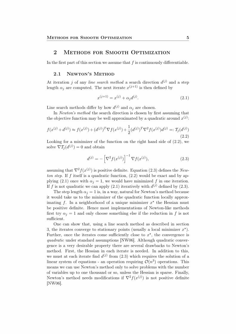
2.2 Quasi-Newton Methods
A standard alternative to Newton’s method is a class of line search methodswhere the search direction is defined by
d(j) = −Cj∇f(x(j)) (2.4)
where Cj is updated in each iteration by a quasi-Newton updating formulain such a way that it has certain properties of the inverse of the true Hessian.
As long as Cj is symmetric positive definite, we have (d(j))T∇f(x(j)) < 0,that is d(j) is a descent direction. If we take Cj = I (the identity matrix),the method reduces to the steepest descent method.
By comparing the quasi-Newton step (2.4) to the Newton step (2.3), wesee that the two are equal when Cj is equal to the inverse Hessian. So takinga quasi-Newton step is the same as minimizing the quadradic function (2.2)with ∇2f(x(j)) replaced by Bj := C−1
j . To update this matrix we imposethe well known secant equation:
Bj+1(αjd(j)) = ∇f(x(j+1))−∇f(x(j)) (2.5)
If we set
s(j) = x(j+1) − x(j) and y(j) = ∇f(x(j+1))−∇f(x(j)) (2.6)
equation (2.5) becomesBj+1s
(j) = y(j) (2.7)
or equivalentlyCj+1y
(j) = s(j). (2.8)
This requirement, together with the requirement that Cj+1 be symmetricpositive definite, is not enough to uniquely determine Cj+1. To do that wefurther require that
Cj+1 = argminC‖C − Cj‖ (2.9)
i.e. that Cj+1, in the sense of some matrix norm, be the closest to Cj amongall symmetric positive definite matrices that satisfy the secant equation (2.8).Each choice of matrix norm gives rise to a different update formula.
2.3 BFGS
The most popular update formula is
CBFGSj+1 =
(I − ρjs(j)(y(j))T
)Cj
(I − ρjy(j)(s(j))T
)+ ρjs
(j)(s(j))T (2.10)
where ρj =((y(j))T s(j)
)−1. Notice that the computation in (2.10) requiresonlyO(n2) operations because Cj
(I − ρjy(j)(s(j))T
)= Cj−ρj(Cjy(j))(s(j))T ,
Methods for Smooth Optimization 7
Algorithm 1 BFGSInput: x(0), δ, C0
j ← 0while true do
d(j) ← −Cj∇f(x(j))αj ← LineSearch(x(j), f)x(j+1) ← x(j) + αjd
(j)
Compute Cj+1 from (2.10) and (2.6)j ← j + 1if ‖∇f(x(j))‖ ≤ δ then
stopend if
end whileOutput: x(j), f(x(j)) and ∇f(x(j)).
a computation that needs one matrix-vector multiplication, one vector outerproduct and one matrix addition.
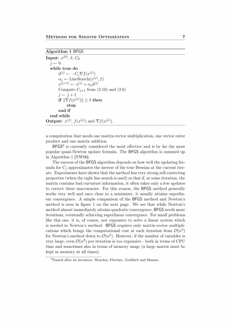
BFGS2 is currently considered the most effective and is by far the mostpopular quasi-Newton update formula. The BFGS algorithm is summed upin Algorithm 1 [NW06].
The success of the BFGS algorithm depends on how well the updating for-mula for Cj approximates the inverse of the true Hessian at the current iter-ate. Experiments have shown that the method has very strong self-correctingproperties (when the right line search is used) so that if, at some iteration, thematrix contains bad curvature information, it often takes only a few updatesto correct these inaccuracies. For this reason, the BFGS method generallyworks very well and once close to a minimizer, it usually attains superlin-ear convergence. A simple comparison of the BFGS method and Newton’smethod is seen in figure 1 on the next page. We see that while Newton’smethod almost immediately attains quadratic convergence, BFGS needs moreiterations, eventually achieving superlinear convergence. For small problemslike this one, it is, of course, not expensive to solve a linear system whichis needed in Newton’s method. BFGS requires only matrix-vector multipli-cations which brings the computational cost at each iteration from O(n3)for Newton’s method down to O(n2). However, if the number of variables isvery large, even O(n2) per iteration is too expensive - both in terms of CPUtime and sometimes also in terms of memory usage (a large matrix must bekept in memory at all times).
2Named after its inventors: Broyden, Fletcher, Goldfarb and Shanno.
Methods for Smooth Optimization 8
−1 −0.5 0 0.5 1 1.5−1
−0.5
0
0.5
1
1.5
BFGSNewton’sLocal Minimizer
(a) Paths followed.
0 2 4 6 8 10 1210
−25
10−20
10−15
10−10
10−5
100
105
BFGSNewton’s
(b) Function value at each iterate.
Figure 1: Results from running BFGS (blue) and Newton’s method (black) on thesmooth 2D Rosenbrock function f(x) = (1−x1)
2+(x2−x21)
2 with x(0) = (−0.9,−0.5).The minimizer is x? = (1, 1) and f(x?) = 0.
2.4 Limited Memory BFGS
A less computationally intensive method when n is large is the Limited-Memory BFGS method (LBFGS), see [Noc80, NW06]. Instead of updatingand storing the entire approximated inverse Hessian Cj , the LBFGS methodnever explicitly forms or stores this matrix. Instead it stores informationfrom the past m iterations and uses only this information to implicitly dooperations requiring the inverse Hessian (in particular computing the nextsearch direction). The first m iterations, LBFGS and BFGS generate thesame search directions (assuming the initial search directions for the twoare identical and that no scaling is done – see section 5.1.5). The updatingin LBFGS is done using just 4mn multiplications (see Algorithm 2 [NW06])bringing the computational cost down to O(mn) per iteration. If m � nthis is effectively the same as O(n). As we shall see later, often LBFGSis successful with m ∈ [2, 35] even when n = 103 or larger. It can alsobe argued that the LBFGS method has the further advantage that it only
Algorithm 2 Direction finding in LBFGS1: q ← γj∇f(x(j)), with γj = ((s(j−1))T y(j−1))((y(j−1))T y(j−1))−1
2: for i = (j − 1) : (−1) : (j −m) do3: αi ← ρi(s(i))T q4: q ← q − αiy(i)
5: end for6: for i = (j −m) : 1 : (j − 1) do7: β ← ρi(y(i))T r8: r ← r + s(i)(αi − β)9: end forOutput: d(j) = −r

Methods for Smooth Optimization 9
−1 −0.5 0 0.5 1 1.5−1
−0.5
0
0.5
1
1.5
BFGSNewton’sLBFGSLocal Minimizer
(a) Paths followed.
0 2 4 6 8 10 1210
−25
10−20
10−15
10−10
10−5
100
105
BFGSNewton’sLBFGS
(b) Function value at each iterate.
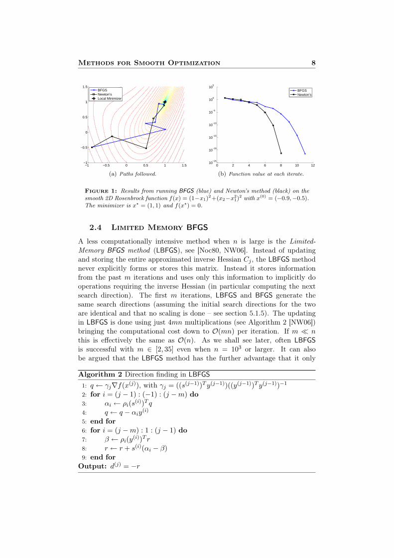
Figure 2: Results from running BFGS (blue), LBFGS with m = 3 (red), andNewton’s method (black) on the smooth 2D Rosenbrock function f(x) = (1 − x1)
2 +(x2 − x2
1)2 with x(0) = (−0.9,−0.5). The minimizer is x? = (1, 1) and f(x?) = 0.
uses relatively new information. In the BFGS method, the inverse Hessiancontains information from all previous iterates. This may be problematic ifthe objective function is very different in nature in different regions.
In some cases the LBFGS method uses as many or even fewer functionevaluations to find the minimizer. This is remarkable considering that evenwhen using the same number of function evaluations, LBFGS runs signifi-cantly faster than full BFGS if n is large.
In figure 2 we see how LBFGS compares to BFGS and Newton’s methodon the same problem as before. We see that for this particular problem,using m = 2, LBFGS performs almost as well as the full BFGS.
Experiments show that the optimal choice of m is problem dependentwhich is a drawback of the LBFGS method. In case of LBFGS failing, oneshould first try to increase m before completely discarding the method. Invery few situations (as we will see later on a nonsmooth example) the LBFGSmethod may needm > n to converge, in which case LBFGS is more expensivethan regular BFGS.
Newton’s BFGS LBFGSWork per iteration O(n3) O(n2) O(mn)
2.5 Applicability to Nonsmooth Optimization
Now suppose that the objective function f is not differentiable everywhere,in particular that it is not differentiable at a minimizer x?.
In Newton and quasi-Newton methods, we assumed that f may be wellapproximated by a quadratic function in a region containing the currentiterate. If we are close to a point of nonsmoothness, this assumption nolonger holds.
Methods for Smooth Optimization 10
When f is locally Lipschitz, we have by Rademacher’s theorem [Cla83]that f is differentiable almost everywhere. Roughly speaking, this meansthat the probability that an optimization algorithm that is initialized ran-domly will encounter a point where f is not differentiable is zero. This iswhat allows us to directly apply optimization algorithms originally designedfor smooth optimization to nonsmooth problems. In fact we are assumingthat we never encounter such a point throughout the rest of this thesis. Thisensures that the methods used stay well defined.
Simple examples show that the steepest descent method may convergeto nonoptimal points when f is nonsmooth [HUL93, LO10] and Newton’smethod is also unsuitable when f is nonsmooth.
2.6 Quasi-Newton Methods in the Nonsmooth Case
Although standard quasi-Newton methods were developed for smooth op-timization it turns out [LO10] that they often succeed in minimizing nons-mooth objective functions when applied directly without modification (whenthe right line search is used — see section 3).
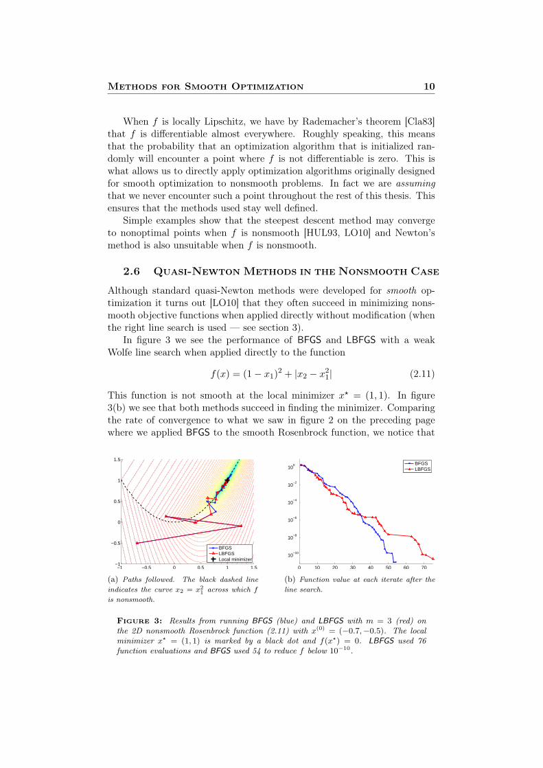
In figure 3 we see the performance of BFGS and LBFGS with a weakWolfe line search when applied directly to the function
f(x) = (1− x1)2 + |x2 − x21| (2.11)
This function is not smooth at the local minimizer x? = (1, 1). In figure3(b) we see that both methods succeed in finding the minimizer. Comparingthe rate of convergence to what we saw in figure 2 on the preceding pagewhere we applied BFGS to the smooth Rosenbrock function, we notice that
−1 −0.5 0 0.5 1 1.5−1
−0.5
0
0.5
1
1.5
BFGSLBFGSLocal minimizer
(a) Paths followed. The black dashed lineindicates the curve x2 = x2
1 across which f
is nonsmooth.
0 10 20 30 40 50 60 70
10−10
10−8
10−6
10−4
10−2
100
BFGSLBFGS
(b) Function value at each iterate after theline search.
Figure 3: Results from running BFGS (blue) and LBFGS with m = 3 (red) onthe 2D nonsmooth Rosenbrock function (2.11) with x(0) = (−0.7,−0.5). The localminimizer x? = (1, 1) is marked by a black dot and f(x?) = 0. LBFGS used 76function evaluations and BFGS used 54 to reduce f below 10−10.

Methods for Smooth Optimization 11
the convergence is now approximately linear instead of superlinear. This isdue to the nonsmoothness of the problem.
Most of the rest of this thesis is concerned with investigating the behaviorof quasi-Newton methods - in particular the LBFGS method - when used fornonsmooth (both convex and nonconvex) optimization. We will show resultsfrom numerous numerical experiments and we will compare a number ofnonsmooth optimization algorithms. First, however, we address the issue ofthe line search in more detail.
Line Search 12
3 Line Search
Once the search direction in a line search method has been found, a procedureto determine how long a step should be taken is needed (see (2.1)).
Assuming the line search method has reached the current iterate x(j) andthat a search direction d(j) has been found, we consider the function
φ(α) = f(x(j) + αd(j)), α ≥ 0 (3.1)
i.e. the value of f from x(j) in the direction of d(j). Since d(j) is a descentdirection, there exists α̂ > 0 small enough that φ(α̂) < f(x(j)). However, fora useful procedure, we need steps ensuring sufficient decrease in the functionvalue and steps that are not too small. If we are using the line search in aquasi-Newton method, we must also ensure that the approximated Hessianmatrix remains positive definite.
3.1 Strong Wolfe Conditions
The Strong Wolfe conditions require that the following two inequalities holdfor αj :
φ(αj) ≤ φ(0) + αjc1φ′(0) Armijo condition (3.2)
|φ′(αj)| ≤ c2|φ′(0)| Strong Wolfe condition (3.3)
with 0 < c1 < c2 < 1. The Armijo condition ensures a sufficient decreasein the function value. Remembering that φ′(0) is negative (because d(j)
is a descent direction), we see that the Armijo condition requires that thedecrease be greater if αj is greater.
(a) Smooth φ(α). (b) nonsmooth φ(α).
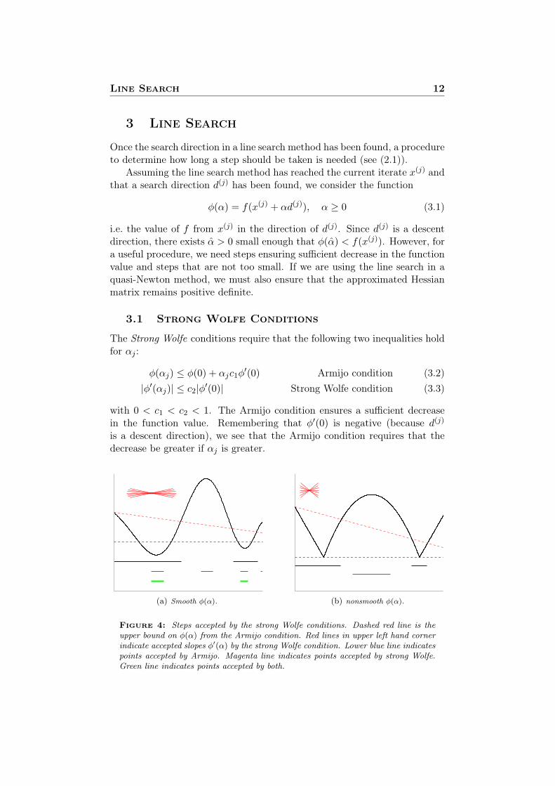
Figure 4: Steps accepted by the strong Wolfe conditions. Dashed red line is theupper bound on φ(α) from the Armijo condition. Red lines in upper left hand cornerindicate accepted slopes φ′(α) by the strong Wolfe condition. Lower blue line indicatespoints accepted by Armijo. Magenta line indicates points accepted by strong Wolfe.Green line indicates points accepted by both.
Line Search 13
The strong Wolfe condition ensures that the derivative φ′(αj) is reducedin absolute value. This makes sense for smooth functions because the deriva-tive at a minimizer of φ(α) would be zero. Figure 4 shows the intervals ofstep lengths accepted by the strong Wolfe line search.
It is clear that the strong Wolfe condition is not useful for nonsmoothoptimization. The requirement (3.3) is bad because for nonsmooth functions,the derivative near a minimizer of φ(α) need not be small in absolute value(see figure 4(b) on the previous page).
3.2 Weak Wolfe Conditions
The Weak Wolfe conditions are
φ(αj) ≤ φ(0) + αjc1φ′(0) Armijo condition (3.4)
φ′(αj) ≥ c2φ′(0) Weak Wolfe condition (3.5)
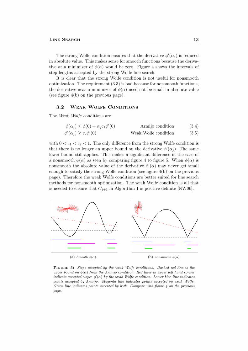
with 0 < c1 < c2 < 1. The only difference from the strong Wolfe condition isthat there is no longer an upper bound on the derivative φ′(αj). The samelower bound still applies. This makes a significant difference in the case ofa nonsmooth φ(α) as seen by comparing figure 4 to figure 5. When φ(α) isnonsmooth the absolute value of the derivative φ′(α) may never get smallenough to satisfy the strong Wolfe condition (see figure 4(b) on the previouspage). Therefore the weak Wolfe conditions are better suited for line searchmethods for nonsmooth optimization. The weak Wolfe condition is all thatis needed to ensure that Cj+1 in Algorithm 1 is positive definite [NW06].
(a) Smooth φ(α). (b) nonsmooth φ(α).
Figure 5: Steps accepted by the weak Wolfe conditions. Dashed red line is theupper bound on φ(α) from the Armijo condition. Red lines in upper left hand cornerindicate accepted slopes φ′(α) by the weak Wolfe condition. Lower blue line indicatespoints accepted by Armijo. Magenta line indicates points accepted by weak Wolfe.Green line indicates points accepted by both. Compare with figure 4 on the previouspage.
Line Search 14
3.3 Bracketing Algorithm
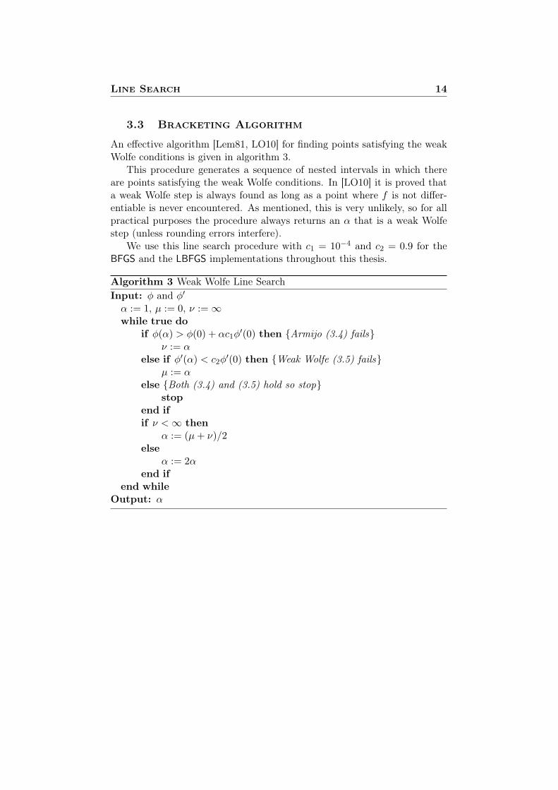
An effective algorithm [Lem81, LO10] for finding points satisfying the weakWolfe conditions is given in algorithm 3.
This procedure generates a sequence of nested intervals in which thereare points satisfying the weak Wolfe conditions. In [LO10] it is proved thata weak Wolfe step is always found as long as a point where f is not differ-entiable is never encountered. As mentioned, this is very unlikely, so for allpractical purposes the procedure always returns an α that is a weak Wolfestep (unless rounding errors interfere).
We use this line search procedure with c1 = 10−4 and c2 = 0.9 for theBFGS and the LBFGS implementations throughout this thesis.
Algorithm 3 Weak Wolfe Line SearchInput: φ and φ′
α := 1, µ := 0, ν :=∞while true do
if φ(α) > φ(0) + αc1φ′(0) then {Armijo (3.4) fails}
ν := αelse if φ′(α) < c2φ
′(0) then {Weak Wolfe (3.5) fails}µ := α
else {Both (3.4) and (3.5) hold so stop}stop
end ifif ν <∞ then
α := (µ+ ν)/2else
α := 2αend if
end whileOutput: α
LBFGS and BFGS for Nonsmooth Optimization 15
4 LBFGS and BFGS for Nonsmooth Opti-mization
That the LBFGS method can be used for nonsmooth optimization may besurprising at first since it was originally developed as a limited memory ver-sion (hence well suited for large-scale problems) of the smooth optimizationalgorithm BFGS. We here present results showing that LBFGS, in fact, workswell for a range of nonsmooth problems. This should be seen as an exten-sion and large-scale version of the numerical results in [LO10] where the fullBFGS method is tested on the same problems.
4.1 Definitions
4.1.1 Random starting points
Whenever we speak of a random starting point, we mean a starting pointx(0) ∈ Rn drawn randomly from the uniform distribution on [−1, 1]n. To dothis we use the built in function rand in Matlab. Exceptions to this rulewill be mentioned explicitly.
4.1.2 Rate of convergence
From this point on, when we refer to the rate of convergence of an algorithmwhen applied to a problem, we mean the R-linear rate of convergence of theerror in function value. Using the terminology of [NW06], this means thereexist constants C > 0 and r ∈ (0, 1) such that
|fk − f?| ≤ Crk (4.1)
The number r is called the rate of convergence. Since equation (4.1) meansthat
log |fk − f?| ≤ logC + k log r
we see that for a rate of convergence r, there is a line with slope log r bound-ing the numbers {log |fk − f?|} above. To estimate the rate of convergenceof fk with respect to a sequence nk, we do a least squares fit to the points(nk, log |fk − f?|) and the slope of the optimal line is then log r.
To get a picture of the performance of the algorithms in terms of a usefulmeasure, we actually use for fk the function value accepted by the line searchat the end of iteration k and for nk the total number of function evaluationsused - including those used by the line search - at the end of iteration k.
For r close to 1, the algorithm converges slowly while it is fast for smallr. For this reason we will, when showing rates of convergence, always plotthe quantity − log (1− r), whose range is (0,∞) and which will be large ifthe algorithm is slow and small if the algorithm is fast.
LBFGS and BFGS for Nonsmooth Optimization 16
4.1.3 V - and U-spaces
Many nonsmooth functions are partly smooth [Lew02]. This concept leads tothe notions of the U - and V -spaces associated with a point – most often theminimizer. In the convex case, this notion was first discussed in [LOS00].
Roughly this concept may be described as follows: Let M be a mani-fold containing x that is such that f restricted to M is twice continuouslydifferentiable. Assume that M is chosen to have maximal dimension, bywhich we mean that its tangent space at x has maximal dimension (n inthe special case that f is a smooth function). Then the subspace tangent toM at x is called the U -space of f at x and its orthogonal complement theV -space. Loosely speaking, we think of the U -space as the subspace spannedby the directions along which f varies smoothly at x and the V -space as itsorthogonal complement. This means that ψ(t) = f(x+ ty) varies smoothlyaround t = 0 only if the component of y in the V -space of f at x vanishes.If not, ψ varies nonsmoothly around t = 0.
Consider the function f(x) = ‖x‖. The minimizer is clearly x = 0. Lety be any unit length vector. Then ψ(t) = f(ty) = |t|‖y‖ = |t| which variesnonsmoothly across t = 0 regardless of y. The U -space of f at x = 0 is thus{0} and the V -space is Rn.
As a second example, consider the nonsmooth Rosenbrock function (2.11).If x2 = x2
1, the second term vanishes so when restricted to the manifoldM = {x : x2 = x2
1}, f is smooth. The subspace tangent toM at the localminimizer (1, 1) is U = {x : x = (1, 2)t, t ∈ R} which is one-dimensional.The orthogonal complement is V = {x : x = (−2, 1)t, t ∈ R} which is alsoone-dimensional.
In [LO10] it is observed that running BFGS produces information aboutthe U− and V -spaces at the minimizer. At a point of nonsmoothness thegradients jump discontinuously. However at a point of nonsmoothness wecan approximate the objective function arbitrarily well by a smooth function.Close to the point of nonsmoothness, the Hessian of that function would haveextremely large eigenvalues to accomodate the rapid change in the gradients.Numerically there is no way to distinguish such a smooth function from theactual nonsmooth objective function (assuming the smooth approximationis sufficiently exact).
When running BFGS, an approximation to the inverse Hessian is contin-uously updated and stored. Very large curvature information in the Hessianof the objective corresponds to very small eigenvalues of the inverse Hessian.Thus, it is observed in [LO10] that one can obtain information about theU− and V -spaces at the minimizer by simply monitoring the eigenvaluesof the inverse Hessian approximation Cj when the iterates get close to theminimizer.

LBFGS and BFGS for Nonsmooth Optimization 17
0 500 1000 150010
−6
10−4
10−2
100
102
(a) LBFGS with m = 15.
0 500 1000 150010
−6
10−4
10−2
100
102
(b) LBFGS with m = 25.
0 500 1000 150010
−6
10−4
10−2
100
102
n = 4n = 8n = 16n = 32n = 64
(c) BFGS.
Figure 6: LBFGS and BFGS on (4.2) for different n. Vertical axis: Function valueat the end of each iteration. Horizontal axis: Total number of function evaluationsused. The number of updates used in LBFGS was m = 25 and x(0) = (1, . . . , 1).
4.2 LBFGS and BFGS on Five Academic Problems
4.2.1 Tilted norm function
We consider the convex function
f(x) = w‖Ax‖+ (w − 1)eT1Ax (4.2)
where e1 is the first unit vector, w = 4 and A is a randomly generatedsymmetric positive definite matrix with condition number n2. This functionis not smooth at its minimizer x? = 0.
In figure 6 we see typical runs of LBFGS and BFGS on (4.2). It is clearfrom figures 6(a) and 6(b) that the performance of LBFGS on this problemdepends on the number of updates m used. We will investigate this furtherin section 4.4.
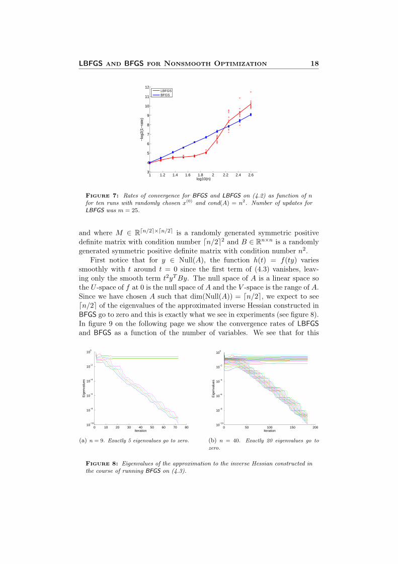
Comparing the three plots in figure 6 we see that the linear rate of con-vergence varies differently with n for LBFGS and BFGS. This is also what wesee in figure 7, where we have shown observed rates of convergence for tenruns with random x(0) for different n. Since all runs were successful for bothLBFGS and BFGS, ten red and ten blue crosses appear on each vertical line.The curves indicate the mean of the observed rates.
We see that for smaller n, LBFGS generally gets better convergence ratesbut gets relatively worse when n increases.
4.2.2 A convex, nonsmooth function
We consider the function
f(x) =√xTAx+ xTBx (4.3)
where we take
A =(M 00 0
)(4.4)
LBFGS and BFGS for Nonsmooth Optimization 18
1 1.2 1.4 1.6 1.8 2 2.2 2.4 2.63
4
5
6
7
8
9
10
11
12
log10(n)
−lo
g2(1
−ra
te)
LBFGSBFGS
Figure 7: Rates of convergence for BFGS and LBFGS on (4.2) as function of nfor ten runs with randomly chosen x(0) and cond(A) = n2. Number of updates forLBFGS was m = 25.
and where M ∈ Rdn/2e×dn/2e is a randomly generated symmetric positivedefinite matrix with condition number dn/2e2 and B ∈ Rn×n is a randomlygenerated symmetric positive definite matrix with condition number n2.
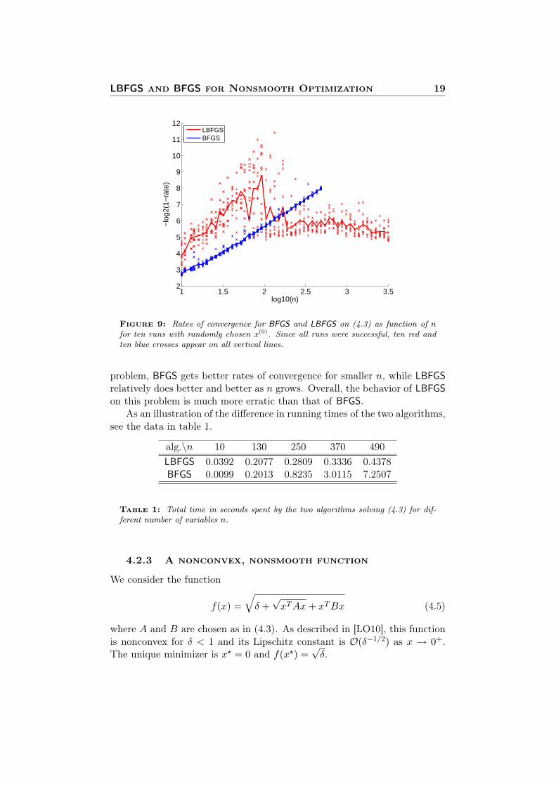
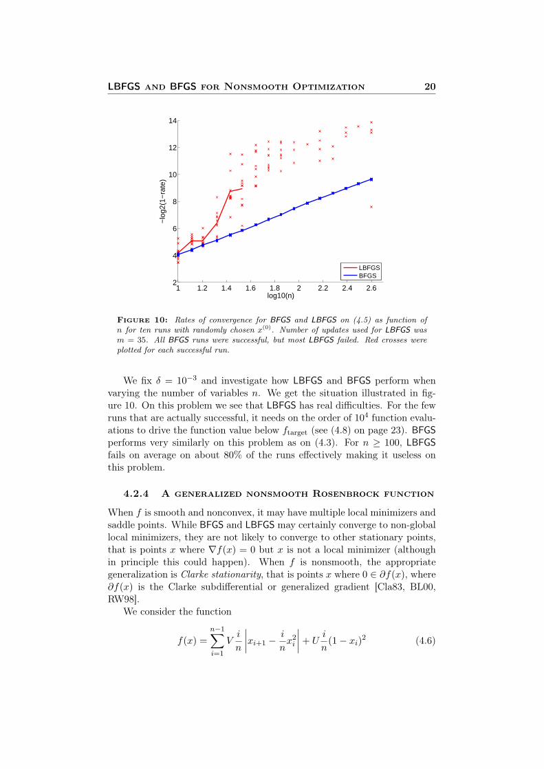
First notice that for y ∈ Null(A), the function h(t) = f(ty) variessmoothly with t around t = 0 since the first term of (4.3) vanishes, leav-ing only the smooth term t2yTBy. The null space of A is a linear space sothe U -space of f at 0 is the null space of A and the V -space is the range of A.Since we have chosen A such that dim(Null(A)) = dn/2e, we expect to seedn/2e of the eigenvalues of the approximated inverse Hessian constructed inBFGS go to zero and this is exactly what we see in experiments (see figure 8).In figure 9 on the following page we show the convergence rates of LBFGSand BFGS as a function of the number of variables. We see that for this
0 10 20 30 40 50 60 70 8010
−10
10−8
10−6
10−4
10−2
100
Iteration
Eig
enva
lues
(a) n = 9. Exactly 5 eigenvalues go to zero.
0 50 100 150 20010
−10
10−8
10−6
10−4
10−2
100
Iteration
Eig
enva
lues
(b) n = 40. Exactly 20 eigenvalues go tozero.
Figure 8: Eigenvalues of the approximation to the inverse Hessian constructed inthe course of running BFGS on (4.3).
LBFGS and BFGS for Nonsmooth Optimization 19
1 1.5 2 2.5 3 3.52
3
4
5
6
7
8
9
10
11
12
log10(n)
−lo
g2(1
−ra
te)
LBFGSBFGS
Figure 9: Rates of convergence for BFGS and LBFGS on (4.3) as function of nfor ten runs with randomly chosen x(0). Since all runs were successful, ten red andten blue crosses appear on all vertical lines.
problem, BFGS gets better rates of convergence for smaller n, while LBFGSrelatively does better and better as n grows. Overall, the behavior of LBFGSon this problem is much more erratic than that of BFGS.
As an illustration of the difference in running times of the two algorithms,see the data in table 1.
alg.\n 10 130 250 370 490LBFGS 0.0392 0.2077 0.2809 0.3336 0.4378BFGS 0.0099 0.2013 0.8235 3.0115 7.2507
Table 1: Total time in seconds spent by the two algorithms solving (4.3) for dif-ferent number of variables n.
4.2.3 A nonconvex, nonsmooth function
We consider the function
f(x) =√δ +√xTAx+ xTBx (4.5)
where A and B are chosen as in (4.3). As described in [LO10], this functionis nonconvex for δ < 1 and its Lipschitz constant is O(δ−1/2) as x → 0+.The unique minimizer is x? = 0 and f(x?) =
√δ.
LBFGS and BFGS for Nonsmooth Optimization 20
1 1.2 1.4 1.6 1.8 2 2.2 2.4 2.62
4
6
8
10
12
14
log10(n)
−lo
g2(1
−ra
te)
LBFGSBFGS
Figure 10: Rates of convergence for BFGS and LBFGS on (4.5) as function ofn for ten runs with randomly chosen x(0). Number of updates used for LBFGS wasm = 35. All BFGS runs were successful, but most LBFGS failed. Red crosses wereplotted for each successful run.
We fix δ = 10−3 and investigate how LBFGS and BFGS perform whenvarying the number of variables n. We get the situation illustrated in fig-ure 10. On this problem we see that LBFGS has real difficulties. For the fewruns that are actually successful, it needs on the order of 104 function evalu-ations to drive the function value below ftarget (see (4.8) on page 23). BFGSperforms very similarly on this problem as on (4.3). For n ≥ 100, LBFGSfails on average on about 80% of the runs effectively making it useless onthis problem.
4.2.4 A generalized nonsmooth Rosenbrock function
When f is smooth and nonconvex, it may have multiple local minimizers andsaddle points. While BFGS and LBFGS may certainly converge to non-globallocal minimizers, they are not likely to converge to other stationary points,that is points x where ∇f(x) = 0 but x is not a local minimizer (althoughin principle this could happen). When f is nonsmooth, the appropriategeneralization is Clarke stationarity, that is points x where 0 ∈ ∂f(x), where∂f(x) is the Clarke subdifferential or generalized gradient [Cla83, BL00,RW98].
We consider the function
f(x) =n−1∑i=1
Vi
n
∣∣∣∣xi+1 −i
nx2i
∣∣∣∣+ Ui
n(1− xi)2 (4.6)
LBFGS and BFGS for Nonsmooth Optimization 21
0 100 200 300 400 500
5.5
6
6.5
7
7.5
8
8.5
9
9.5
Diff. starting points
ffina
l
(a) BFGS
0 100 200 300 400 500
5.5
6
6.5
7
7.5
8
8.5
9
9.5
Diff. starting points
ffina
l
(b) LBFGS with m = 30
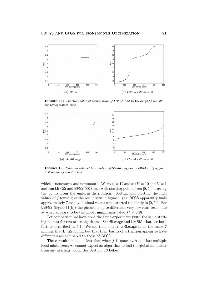
Figure 11: Function value at termination of LBFGS and BFGS on (4.6) for 500randomly started runs.
0 100 200 300 400 500
5.5
6
6.5
7
7.5
8
8.5
9
9.5
Diff. starting points
ffina
l
(a) ShorRLesage
0 100 200 300 400 5005
6
7
8
9
10
11
12
13
14
15
Diff. starting points
ffina
l
(b) LMBM with m = 30
Figure 12: Function value at termination of ShorRLesage and LMBM on (4.6) for500 randomly started runs.
which is nonconvex and nonsmooth. We fix n = 12 and set V = 10 and U = 1and run LBFGS and BFGS 500 times with starting points from [0, 5]n drawingthe points from the uniform distribution. Sorting and plotting the finalvalues of f found give the result seen in figure 11(a). BFGS apparently findsapproximately 7 locally minimal values when started randomly in [0, 5]n. ForLBFGS (figure 11(b)) the picture is quite different. Very few runs terminateat what appears to be the global minimizing value f? ≈ 5.38.
For comparison we have done the same experiment (with the same start-ing points) for two other algorithms, ShorRLesage and LMBM, that are bothfurther described in 5.1. We see that only ShorRLesage finds the same 7minima that BFGS found, but that their basins of attraction appear to havedifferent sizes compared to those of BFGS.
These results make it clear that when f is nonconvex and has multiplelocal minimizers, we cannot expect an algorithm to find the global minimizerfrom any starting point. See Section 4.3 below.
LBFGS and BFGS for Nonsmooth Optimization 22
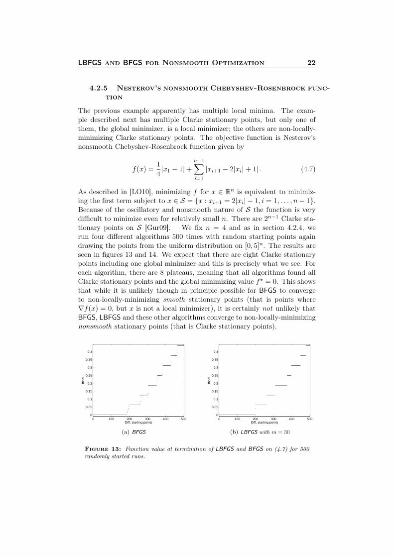
4.2.5 Nesterov’s nonsmooth Chebyshev-Rosenbrock func-tion
The previous example apparently has multiple local minima. The exam-ple described next has multiple Clarke stationary points, but only one ofthem, the global minimizer, is a local minimizer; the others are non-locally-minimizing Clarke stationary points. The objective function is Nesterov’snonsmooth Chebyshev-Rosenbrock function given by
f(x) =14|x1 − 1|+
n−1∑i=1
|xi+1 − 2|xi|+ 1| . (4.7)
As described in [LO10], minimizing f for x ∈ Rn is equivalent to minimiz-ing the first term subject to x ∈ S = {x : xi+1 = 2|xi| − 1, i = 1, . . . , n− 1}.Because of the oscillatory and nonsmooth nature of S the function is verydifficult to minimize even for relatively small n. There are 2n−1 Clarke sta-tionary points on S [Gur09]. We fix n = 4 and as in section 4.2.4, werun four different algorithms 500 times with random starting points againdrawing the points from the uniform distribution on [0, 5]n. The results areseen in figures 13 and 14. We expect that there are eight Clarke stationarypoints including one global minimizer and this is precisely what we see. Foreach algorithm, there are 8 plateaus, meaning that all algorithms found allClarke stationary points and the global minimizing value f? = 0. This showsthat while it is unlikely though in principle possible for BFGS to convergeto non-locally-minimizing smooth stationary points (that is points where∇f(x) = 0, but x is not a local minimizer), it is certainly not unlikely thatBFGS, LBFGS and these other algorithms converge to non-locally-minimizingnonsmooth stationary points (that is Clarke stationary points).
0 100 200 300 400 5000
0.05
0.1
0.15
0.2
0.25
0.3
0.35
0.4
Diff. starting points
ffina
l
(a) BFGS
0 100 200 300 400 5000
0.05
0.1
0.15
0.2
0.25
0.3
0.35
0.4
Diff. starting points
ffina
l
(b) LBFGS with m = 30
Figure 13: Function value at termination of LBFGS and BFGS on (4.7) for 500randomly started runs.
LBFGS and BFGS for Nonsmooth Optimization 23
0 100 200 300 400 5000
0.05
0.1
0.15
0.2
0.25
0.3
0.35
0.4
Diff. starting points
ffina
l
(a) ShorRLesage
0 100 200 300 400 5000
0.05
0.1
0.15
0.2
0.25
0.3
0.35
0.4
Diff. starting points
ffina
l
(b) LMBM with m = 30
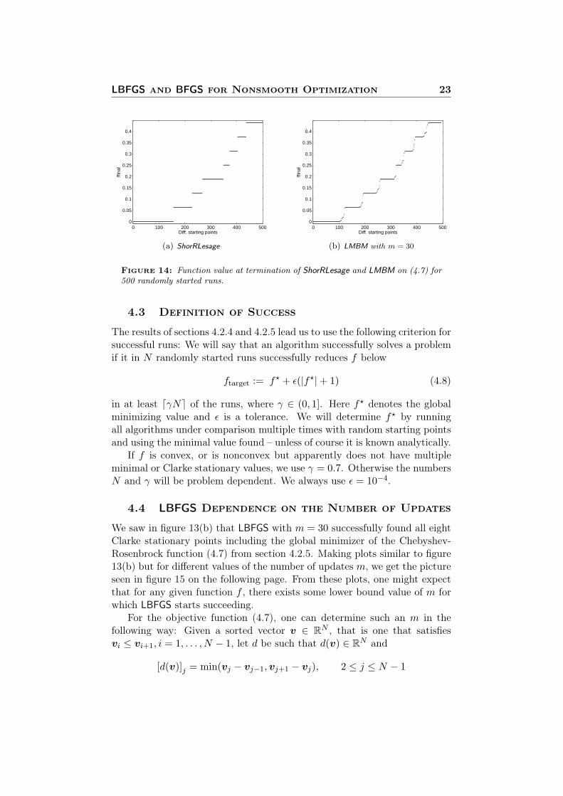
Figure 14: Function value at termination of ShorRLesage and LMBM on (4.7) for500 randomly started runs.
4.3 Definition of Success
The results of sections 4.2.4 and 4.2.5 lead us to use the following criterion forsuccessful runs: We will say that an algorithm successfully solves a problemif it in N randomly started runs successfully reduces f below
ftarget := f? + ε(|f?|+ 1) (4.8)
in at least dγNe of the runs, where γ ∈ (0, 1]. Here f? denotes the globalminimizing value and ε is a tolerance. We will determine f? by runningall algorithms under comparison multiple times with random starting pointsand using the minimal value found – unless of course it is known analytically.
If f is convex, or is nonconvex but apparently does not have multipleminimal or Clarke stationary values, we use γ = 0.7. Otherwise the numbersN and γ will be problem dependent. We always use ε = 10−4.
4.4 LBFGS Dependence on the Number of Updates
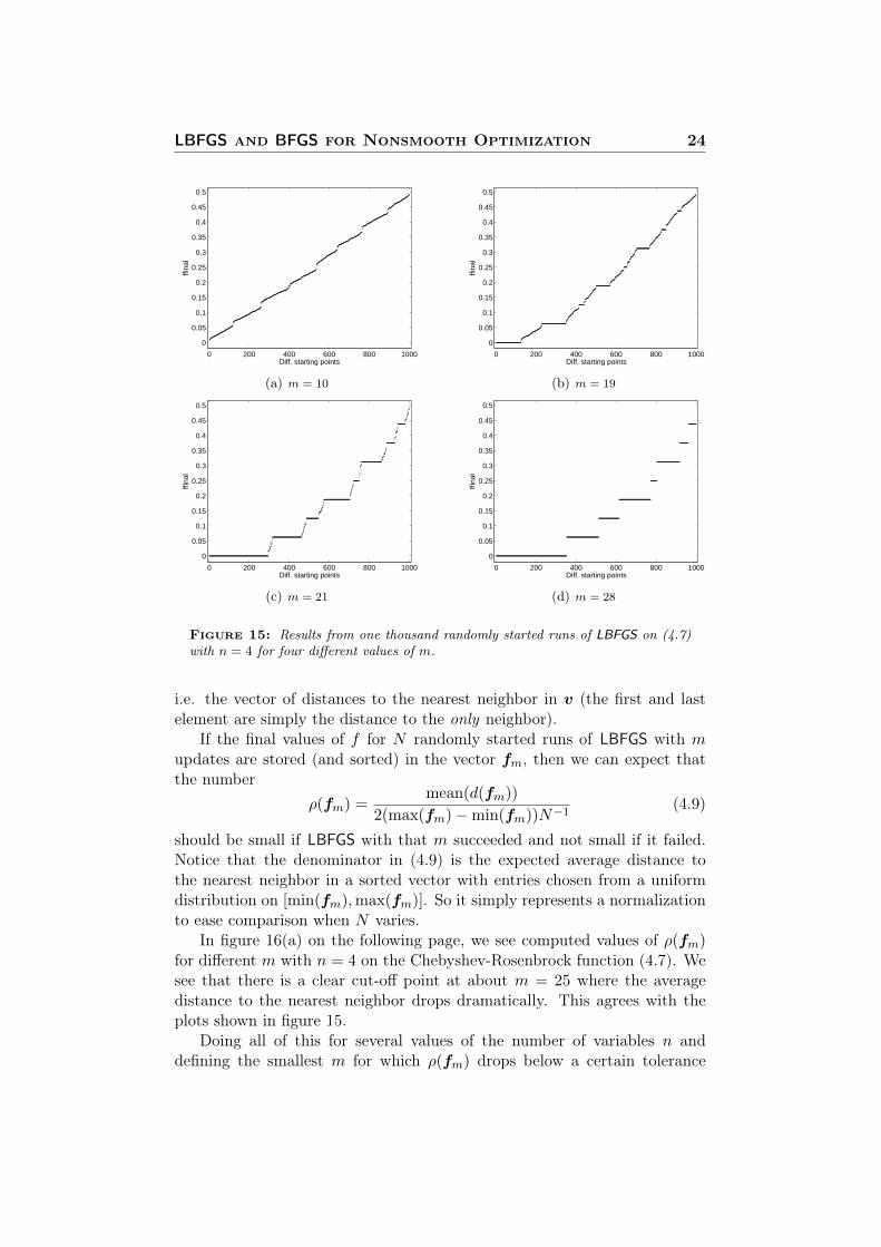
We saw in figure 13(b) that LBFGS with m = 30 successfully found all eightClarke stationary points including the global minimizer of the Chebyshev-Rosenbrock function (4.7) from section 4.2.5. Making plots similar to figure13(b) but for different values of the number of updates m, we get the pictureseen in figure 15 on the following page. From these plots, one might expectthat for any given function f , there exists some lower bound value of m forwhich LBFGS starts succeeding.
For the objective function (4.7), one can determine such an m in thefollowing way: Given a sorted vector v ∈ RN , that is one that satisfiesvi ≤ vi+1, i = 1, . . . , N − 1, let d be such that d(v) ∈ RN and
[d(v)]j = min(vj − vj−1,vj+1 − vj), 2 ≤ j ≤ N − 1
LBFGS and BFGS for Nonsmooth Optimization 24
0 200 400 600 800 1000
0
0.05
0.1
0.15
0.2
0.25
0.3
0.35
0.4
0.45
0.5
Diff. starting points
ffina
l
(a) m = 10
0 200 400 600 800 1000
0
0.05
0.1
0.15
0.2
0.25
0.3
0.35
0.4
0.45
0.5
Diff. starting points
ffina
l
(b) m = 19
0 200 400 600 800 1000
0
0.05
0.1
0.15
0.2
0.25
0.3
0.35
0.4
0.45
0.5
Diff. starting points
ffina
l
(c) m = 21
0 200 400 600 800 1000
0
0.05
0.1
0.15
0.2
0.25
0.3
0.35
0.4
0.45
0.5
Diff. starting points
ffina
l
(d) m = 28
Figure 15: Results from one thousand randomly started runs of LBFGS on (4.7)with n = 4 for four different values of m.
i.e. the vector of distances to the nearest neighbor in v (the first and lastelement are simply the distance to the only neighbor).
If the final values of f for N randomly started runs of LBFGS with mupdates are stored (and sorted) in the vector fm, then we can expect thatthe number
ρ(fm) =mean(d(fm))
2(max(fm)−min(fm))N−1(4.9)
should be small if LBFGS with that m succeeded and not small if it failed.Notice that the denominator in (4.9) is the expected average distance tothe nearest neighbor in a sorted vector with entries chosen from a uniformdistribution on [min(fm),max(fm)]. So it simply represents a normalizationto ease comparison when N varies.
In figure 16(a) on the following page, we see computed values of ρ(fm)for different m with n = 4 on the Chebyshev-Rosenbrock function (4.7). Wesee that there is a clear cut-off point at about m = 25 where the averagedistance to the nearest neighbor drops dramatically. This agrees with theplots shown in figure 15.
Doing all of this for several values of the number of variables n anddefining the smallest m for which ρ(fm) drops below a certain tolerance
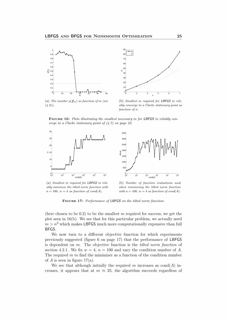
LBFGS and BFGS for Nonsmooth Optimization 25
0 10 20 30 40 50 600
0.1
0.2
0.3
0.4
0.5
0.6
0.7
0.8
0.9
1
m
ρ(f m
)
(a) The number ρ(fm) as function of m (see(4.9)).
2 3 4 5 6 70
10
20
30
40
50
60
70
80
90
n
m
mn2
(b) Smallest m required for LBFGS to reli-ably converge to a Clarke stationary point asfunction of n.
Figure 16: Plots illustrating the smallest necessary m for LBFGS to reliably con-verge to a Clarke stationary point of (4.7) on page 22.
101
102
103
104
105
106
0
5
10
15
20
25
30
cond(A)
m
(a) Smallest m required for LBFGS to reli-ably minimize the tilted norm function withn = 100, w = 4 as function of cond(A).
101
102
103
104
105
106
0
500
1000
1500
2000
2500
3000
3500
cond(A)
nfev
al
(b) Number of function evaluations usedwhen minimizing the tilted norm functionwith n = 100, w = 4 as function of cond(A).
Figure 17: Performance of LBFGS on the tilted norm function.
(here chosen to be 0.2) to be the smallest m required for success, we get theplot seen in 16(b). We see that for this particular problem, we actually needm > n2 which makes LBFGS much more computationally expensive than fullBFGS.
We now turn to a different objective function for which experimentspreviously suggested (figure 6 on page 17) that the performance of LBFGSis dependent on m. The objective function is the tilted norm function ofsection 4.2.1. We fix w = 4, n = 100 and vary the condition number of A.The required m to find the minimizer as a function of the condition numberof A is seen in figure 17(a).
We see that although initially the required m increases as cond(A) in-creases, it appears that at m ≈ 25, the algorithm succeeds regardless of

LBFGS and BFGS for Nonsmooth Optimization 26
cond(A). Figure 17(b) on the previous page also seems to confirm this: Fromabout cond(A) ≈ 103 andm ≈ 25 the number of function evaluations neededto minimize the function does not significantly increase although there arefluctuations.
Comparison of LBFGS and Other Methods 27
5 Comparison of LBFGS and Other Meth-ods
5.1 Other Methods in Comparison
To get a meaningful idea of the performance of LBFGS it must be comparedto other currently used algorithms for the same purpose. The real strength ofLBFGS is the fact that it only uses O(n) operations in each iteration (whenm� n) and so it is specifically useful for large-scale problems – i.e. problemswhere n is of the order of magnitude ≥ 103. The only other method that weknow capable of feasibly solving nonsmooth nonconvex problems of this size,and for which we have access to an implementation, is the LMBM methodpresented in [HMM04]. This means that for large-scale problems, we haveonly one method to compare against. To get a more complete comparison wealso compare LBFGS to other nonsmooth optimization algorithms for small-and medium-scale problems.
5.1.1 LMBM
The Limited Memory Bundle Method (LMBM) was introduced in [HMM04].The method is a hybrid of the bundle method and the limited memoryvariable metric methods (specifically LBFGS). It exploits the ideas of thevariable metric bundle method [HUL93, LV99, Kiw85], namely the utilizationof null steps and simple aggregation of subgradients, but the search directionis calculated using a limited memory approach as in the LBFGS method.Therefore, no time-consuming quadratic program needs to be solved to finda search direction and the number of stored subgradients does not dependon the dimension of the problem. These characteristics make LMBM wellsuited for large-scale problems and it is the only one (other than LBFGS)with that property among the algorithms in comparison.
We used the default parameters except the maximal bundle size, calledna. Since it was demonstrated in [HMM04] that LMBM on the tested prob-lems did as well or even slightly better with na = 10 than with na = 100,we use na = 10.
Fortran code and a Matlab mex-interface for LMBM are currently avail-able at M. Karmitsa’s website3.
5.1.2 RedistProx
The Redistributed Proximal Bundle Method (RedistProx) introduced in [HS09]by Hare and Sagastizábal is aimed at nonconvex, nonsmooth optimization.It uses an approach based on generating cutting-plane models, not of the ob-jective function, but of a local convexification of the objective function. The
3http://napsu.karmitsa.fi/
Comparison of LBFGS and Other Methods 28
corresponding convexification parameter is calculated adaptively “on the fly”.It solves a quadratic minimization problem to find the next search directionwhich typically requires O(n3) operations. To solve this quadratic program,we use the MOSEK QP-solver [MOS03], which gave somewhat better resultsthan using the QP-solver in the Matlab Optimization Toolbox.
RedistProx is not currently publicly available. It was kindly provided tous by the authors to include in our tests. The authors note that this codeis a preliminary implementation of the algorithm and was developed as aproof-of-concept. Future implementations may produce improvement in itsresults.
5.1.3 ShorR
The Shor-R algorithm dates to the 1980s [Sho85]. Its appeal is that it iseasy to describe and implement. It depends on a parameter β, equivalently1 − γ [BLO08], which must be chosen in [0, 1]. When β = 1 (γ = 0), themethod reduces to the steepest descent method, while for β = 0 (γ = 1)it is a variant of the conjugate gradient method. We fix β = γ = 1/2 andfollow the basic definition in [BLO08], using the weak Wolfe line search ofsection 3.3. However, we found that ShorR frequently failed unless the Wolfeparameter c2 was set to a much smaller value than the 0.9 used for BFGSand LBFGS, so that the directional derivative is forced to change sign inthe line search. We used c1 = c2 = 0. The algorithm uses matrix-vectormultiplication and the cost is O(n2) per iteration. The code is available atthe website mentioned in the introduction of this thesis.
5.1.4 ShorRLesage
We include this modified variant of the Shor-R algorithm written by Lesage,based on ideas in [KK00]. The code, which is much more complicated thanthe basic ShorR code, is publicly available on Lesage’s website4.
5.1.5 BFGS
We include also the classical BFGS method originally introduced by Broyden,Fletcher, Goldfarb and Shanno [Bro70, Fle70, Gol70, Sha70]. The methodis described in section 2.2 and experiments regarding its performance onnonsmooth examples were done by Lewis and Overton in [LO10].
We use the same line search as for the LBFGS method (described insection 3.3 and Algorithm 3) and we take C0 = ‖∇f(x(0))‖−1I and scaleC1 by γ = ((s(0))T y(0))((y(0))T y(0))−1 after the first step as suggested in[NW06]. This same scaling is also suggested in [NW06] for LBFGS but beforeevery update. BFGS and LBFGS are only equivalent the first m (the number
4http://www.business.txstate.edu/users/jl47/
Comparison of LBFGS and Other Methods 29
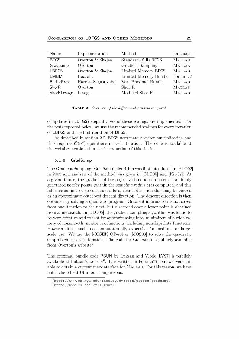
Name Implementation Method LanguageBFGS Overton & Skajaa Standard (full) BFGS MatlabGradSamp Overton Gradient Sampling MatlabLBFGS Overton & Skajaa Limited Memory BFGS MatlabLMBM Haarala Limited Memory Bundle Fortran77RedistProx Hare & Sagastizábal Var. Proximal Bundle MatlabShorR Overton Shor-R MatlabShorRLesage Lesage Modified Shor-R Matlab
Table 2: Overview of the different algorithms compared.
of updates in LBFGS) steps if none of these scalings are implemented. Forthe tests reported below, we use the recommended scalings for every iterationof LBFGS and the first iteration of BFGS.
As described in section 2.2, BFGS uses matrix-vector multiplication andthus requires O(n2) operations in each iteration. The code is available atthe website mentioned in the introduction of this thesis.
5.1.6 GradSamp
The Gradient Sampling (GradSamp) algorithm was first introduced in [BLO02]in 2002 and analysis of the method was given in [BLO05] and [Kiw07]. Ata given iterate, the gradient of the objective function on a set of randomlygenerated nearby points (within the sampling radius ε) is computed, and thisinformation is used to construct a local search direction that may be viewedas an approximate ε-steepest descent direction. The descent direction is thenobtained by solving a quadratic program. Gradient information is not savedfrom one iteration to the next, but discarded once a lower point is obtainedfrom a line search. In [BLO05], the gradient sampling algorithm was found tobe very effective and robust for approximating local minimizers of a wide va-riety of nonsmooth, nonconvex functions, including non-Lipschitz functions.However, it is much too computationally expensive for medium- or large-scale use. We use the MOSEK QP-solver [MOS03] to solve the quadraticsubproblem in each iteration. The code for GradSamp is publicly availablefrom Overton’s website5.
The proximal bundle code PBUN by Lukšan and Vlček [LV97] is publiclyavailable at Luksan’s website6. It is written in Fortran77, but we were un-able to obtain a current mex-interface for Matlab. For this reason, we havenot included PBUN in our comparisons.
5http://www.cs.nyu.edu/faculty/overton/papers/gradsamp/6http://www.cs.cas.cz/luksan/
Comparison of LBFGS and Other Methods 30
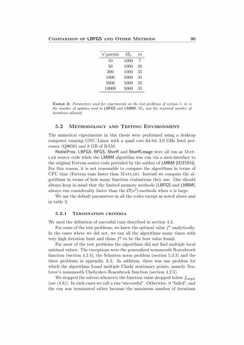
n\param Mit m
10 1000 750 1000 20200 1000 351000 5000 355000 5000 3510000 5000 35
Table 3: Parameters used for experiments on the test problems of section 5. m isthe number of updates used in LBFGS and LMBM. Mit was the maximal number ofiterations allowed.
5.2 Methodology and Testing Environment
The numerical experiments in this thesis were performed using a desktopcomputer running GNU/Linux with a quad core 64-bit 3.0 GHz Intel pro-cessor (Q9650) and 8 GB of RAM.
RedistProx, LBFGS, BFGS, ShorR and ShorRLesage were all run as Mat-lab source code while the LMBM algorithm was run via a mex-interface tothe original Fortran source code provided by the author of LMBM [HMM04].For this reason, it is not reasonable to compare the algorithms in terms ofCPU time (Fortran runs faster than Matlab). Instead we compare the al-gorithms in terms of how many function evaluations they use. One shouldalways keep in mind that the limited memory methods (LBFGS and LMBM)always run considerably faster than the O(n2)-methods when n is large.
We use the default parameters in all the codes except as noted above andin table 3.
5.2.1 Termination criteria
We used the definition of succesful runs described in section 4.3.For some of the test problems, we knew the optimal value f? analytically.
In the cases where we did not, we ran all the algorithms many times withvery high iteration limit and chose f? to be the best value found.
For most of the test problems the algorithms did not find multiple localminimal values. The exceptions were the generalized nonsmooth Rosenbrockfunction (section 4.2.4), the Schatten norm problem (section 5.3.3) and thethree problems in appendix A.3. In addition, there was one problem forwhich the algorithms found multiple Clarke stationary points, namely Nes-terov’s nonsmooth Chebyshev-Rosenbrock function (section 4.2.5).
We stopped the solvers whenever the function value dropped below ftarget(see (4.8)). In such cases we call a run “successful”. Otherwise, it “failed”, andthe run was terminated either because the maximum number of iterations

Comparison of LBFGS and Other Methods 31
Mit was reached or one of the following solver-specific events occurred:
• LBFGS, BFGS and ShorR
1. Line search failed to find acceptable step
2. Search direction was not a descent direction (due to roundingerrors)
3. Step size was less than a certain tolerance: α ≤ εα
• RedistProx
1. Maximum number of restarts reached indicating no further progresspossible
2. Encountered “bad QP” indicating no further progress possible.Usually this is due to a non-positive definite Hessian occuringbecause of rounding errors.
• ShorRLesage
1. Step size was less than a certain tolerance: α ≤ εα
• GradSamp
1. Line search failed to find acceptable step
2. Search direction was not a descent direction (due to roundingerrors)
• LMBM
1. Change in function value was less than a certain tolerance (useddefault value) for 10 consecutive iterations, indicating no furtherprogress possible
2. Maximum number of restarts reached indicating no further progresspossible
5.3 Three Matrix Problems
We now consider three nonsmooth optimization problems arising from matrixapplications. For the problems in this section, we use Mit = 20000.
5.3.1 An eigenvalue problem
We first consider a nonconvex relaxation of an entropy minimization problemtaken from [LO10]. The objective function to be minimized is
f(X) = logEK(A ◦X) (5.1)
Comparison of LBFGS and Other Methods 32
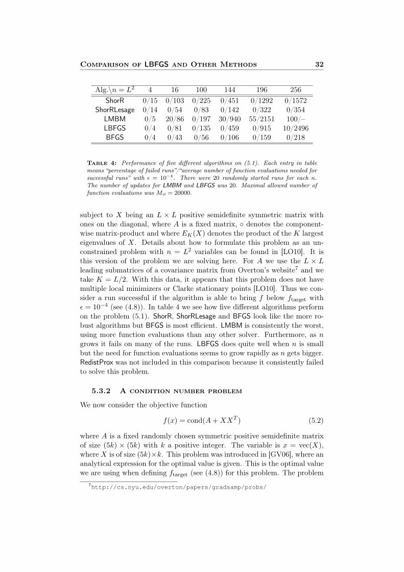
Alg.\n = L2 4 16 100 144 196 256ShorR 0/15 0/103 0/225 0/451 0/1292 0/1572
ShorRLesage 0/14 0/54 0/83 0/142 0/322 0/354LMBM 0/5 20/86 0/197 30/940 55/2151 100/–LBFGS 0/4 0/81 0/135 0/459 0/915 10/2496BFGS 0/4 0/43 0/56 0/106 0/159 0/218
Table 4: Performance of five different algorithms on (5.1). Each entry in tablemeans “percentage of failed runs”/“average number of function evaluations needed forsuccessful runs” with ε = 10−4. There were 20 randomly started runs for each n.The number of updates for LMBM and LBFGS was 20. Maximal allowed number offunction evaluations was Mit = 20000.
subject to X being an L × L positive semidefinite symmetric matrix withones on the diagonal, where A is a fixed matrix, ◦ denotes the component-wise matrix-product and where EK(X) denotes the product of the K largesteigenvalues of X. Details about how to formulate this problem as an un-constrained problem with n = L2 variables can be found in [LO10]. It isthis version of the problem we are solving here. For A we use the L × Lleading submatrices of a covariance matrix from Overton’s website7 and wetake K = L/2. With this data, it appears that this problem does not havemultiple local minimizers or Clarke stationary points [LO10]. Thus we con-sider a run successful if the algorithm is able to bring f below ftarget withε = 10−4 (see (4.8)). In table 4 we see how five different algorithms performon the problem (5.1). ShorR, ShorRLesage and BFGS look like the more ro-bust algorithms but BFGS is most efficient. LMBM is consistently the worst,using more function evaluations than any other solver. Furthermore, as ngrows it fails on many of the runs. LBFGS does quite well when n is smallbut the need for function evaluations seems to grow rapidly as n gets bigger.RedistProx was not included in this comparison because it consistently failedto solve this problem.
5.3.2 A condition number problem
We now consider the objective function
f(x) = cond(A+XXT ) (5.2)
where A is a fixed randomly chosen symmetric positive semidefinite matrixof size (5k) × (5k) with k a positive integer. The variable is x = vec(X),whereX is of size (5k)×k. This problem was introduced in [GV06], where ananalytical expression for the optimal value is given. This is the optimal valuewe are using when defining ftarget (see (4.8)) for this problem. The problem
7http://cs.nyu.edu/overton/papers/gradsamp/probs/

Comparison of LBFGS and Other Methods 33
50 100 150 200 250 300 350 400 450 500
1.2
1.4
1.6
1.8
2
2.2
2.4
2.6
2.8
3
n
log1
0(nf
eval
)
ShorRShorRLesageLMBMLBFGSBFGS
Figure 18: Number of function evaluations required by five different algorithms tobring f in (5.2) below ftarget (defined in (4.8)). There were N = 20 runs for eachalgorithm and we used Mit = 20000.
Alg.\n 45 80 125 180 245 320 405 500ShorR 0/39 0/66 0/96 0/156 0/200 0/327 0/437 0/605
ShorRLesage 0/57 0/65 0/70 0/74 0/75 0/81 0/85 0/88LMBM 0/23 0/33 0/43 0/61 0/67 0/85 0/103 0/125LBFGS 0/22 0/27 0/34 0/44 0/46 0/58 0/62 0/73BFGS 0/35 0/57 0/84 0/131 0/154 0/223 0/276 0/342
Table 5: Performance of five different algorithms on (5.2). Read the table liketable 4 on the preceding page. We used ε = 10−4 and there were 20 randomly startedruns for each n. Number of updates for LMBM and LBFGS was 35.
does not seem to have local minimizers which was confirmed by numerousnumerical experiments similar to those carried out in sections 4.2.4 and 4.2.5.
Table 5 shows the average number of function evaluations required byfive different algorithms to reduce f below ftarget with ε = 10−4 in N = 20randomly started runs for different n. We used n = 5k2, k = 3, 4, . . . , 10.The algorithm RedistProx was not included in this comparison because itconsistently failed to solve this problem. For this problem, LBFGS usedfewer function evaluations than any other algorithm tested. Unlike the othermethods, the number of function evaluations used by ShorRLesage is rela-tively independent of n, making it inefficient for small n but relatively goodfor large n. The condition number of a matrix is strongly pseudoconvex onmatrix space [MY09], and this may explain why all runs were successful for
Comparison of LBFGS and Other Methods 34
all algorithms except RedistProx.
5.3.3 The Schatten norm problem
We now consider the problem
f(x) = ρ‖Ax− b‖2 +n∑j=1
(σj(X))p (5.3)
where x = vec(X) and σk(X) denotes the k’th largest singular value of X.The first term is a penalty term enforcing the linear constraints Ax = b. Thenumber p ∈ (0, 1] is a parameter. If p = 1, the problem is the convex nuclearnorm problem that has received much attention recently, see e.g. [CR08].For p < 1, f is nonconvex and not Lipschitz (when σ → 0+ the gradientexplodes because it involves expressions of the type σp−1). For this reason,one might expect that this problem is very difficult to minimize for p < 1.
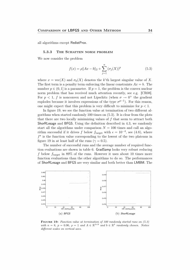
In figure 19, we see the function value at termination of two different al-gorithms when started randomly 100 times on (5.3). It is clear from the plotsthat there are two locally minimizing values of f that seem to attract bothShorRLesage and BFGS. Using the definition described in 4.3, we randomlystart all the algorithms under comparison N = 100 times and call an algo-rithm successful if it drives f below ftarget with ε = 10−4, see (4.8), wheref? is the function value corresponding to the lowest of the two plateaus infigure 19 in at least half of the runs (γ = 0.5).
The number of successful runs and the average number of required func-tion evaluations are shown in table 6. GradSamp looks very robust reducingf below ftarget in 89% of the runs. However it uses about 10 times morefunction evaluations than the other algorithms to do so. The performancesof ShorRLesage and BFGS are very similar and both better than LMBM. The
0 20 40 60 80 100
0.474
0.475
0.476
0.477
0.478
0.479
0.48
0.481
0.482
Diff. starting points
ffina
l
(a) BFGS
0 20 40 60 80 100
0.474
0.475
0.476
0.477
0.478
0.479
Diff. starting points
ffina
l
(b) ShorRLesage
Figure 19: Function value at termination of 100 randomly started runs on (5.3)with n = 8, p = 0.90, ρ = 1 and A ∈ R4×8 and b ∈ R4 randomly chosen. Noticedifferent scales on vertical axes.

Comparison of LBFGS and Other Methods 35
Alg. ffinal ≤ ftarget Succ. Avg. func. eval.ShorR 20% − −
ShorRLesage 68% + 365LMBM 51% + 410LBFGS 0% − −BFGS 62% + 332
GradSamp 89% + 3202RedistProx 0% − −
Table 6: Results of 100 randomly started runs on (5.3) with n = 8, p = 0.90and ρ = 1. A ∈ R4×8 and b ∈ R4 were randomly chosen from a standard normaldistribution. We used Mit = 20000.
remaining three algorithms all fail to get f below ftarget in more than 50%of the runs.
5.4 Comparisons via Performance Profiles
5.4.1 Performance profiles
To better compare the performance of the different methods we use perfor-mance profiles which were introduced in [DM02].
Let P = {p1, p2, . . . } be a set of problems and let S = {s1, s2, . . . } be aset of solvers. If we want to compare the performance of the solvers in S onthe problems in P, we proceed as follows:
Let ap,s denote the absolute amount of computational resource (e.g. CPUtime, memory or number of function evaluations) required by solver s to solveproblem p. If s fails to solve p then we set ap,s =∞.
Let mp denote the least amount of computational resource required byany solver in the comparison to solve problem p, i.e. mp = mins∈S{ap,s} andset rp,s = ap,s/mp. The performance profile for solver s is then
ρs(τ) =|{p ∈ P : log2(rp,s) ≤ τ}|
|P|. (5.4)
Consider the performance profile in figure 20 on the next page. Let us lookat just one solver s. For τ = 0 the numerator in (5.4) is the number ofproblems such that log2(rp,s) ≤ 0. This is only satisfied if rp,s = 1 (becausewe always have rp,s ≥ 1). When rp,s = 1, we have ap,s = mp meaning thatsolver s was best for ρs(0) of all the problems. In figure 20 on the followingpage we see that Solver 4 was best for about 56% of the problems, Solver 2was best for about 44% of the problems and Solvers 1 and 3 were best fornone of the problems.
At the other end of the horizontal axis we see that ρs denotes the fractionof problems which solver s succeeded in solving. If the numerator in (5.4) is

Comparison of LBFGS and Other Methods 36
0 0.5 1 1.5 2 2.5 3 3.50
0.1
0.2
0.3
0.4
0.5
0.6
0.7
0.8
0.9
1
τ
ρ
Solver 1Solver 2Solver 3Solver 4
Figure 20: Example of performance profile.
not equal to |P| when τ is very large, then this means there were problemsthat the solver failed to solve. In figure 20 we see that solvers 1 and 4 solvedall problems while solvers 2 and 3 solved 89% of the problems.
Generally we can read directly off the performance profile graphs therelative performance of the solvers: The higher the performance profile thebetter the corresponding solver. In figure 20, we therefore see that Solver 4overall does best.
In all the performance profiles that follow the computational resourcethat is measured is the number of function evaluations.
5.4.2 Nonsmooth test problems F1–F9
We now present results from applying the seven (six when n > 10) algorithmsto the test problems seen in appendix A.1 on page 45. These problemswere taken from [HMM04] and they can all be defined with any number ofvariables. In table 7 on the following page information about the problems isseen. In table 3 on page 30 we see what parameters were used when solvingthe problems.
The first five problems F1-F5 are convex and the remaining four F6-F9are not convex. We have determined through experiments that apparentlynone of these nonconvex problems have multiple local minima at least forn ≤ 200. In [HMM04] the same nine problems plus one additional problemwere used in comparisons. However, because that additional problem hasseveral local minima, we have moved that problem to a different profile – seesection 5.4.4.
We run all the algorithms N = 10 times with randomly chosen starting

Comparison of LBFGS and Other Methods 37
Problem Convex f?
F1 + 0F2 + 0F3 + −(n− 1)/2F4 + 2(n− 1)F5 + 2(n− 1)F6 − 0F7 − 0F8 − –F9 − 0
Table 7: Information about the problems F1-F9. The column Cvx. indicateswhether or not the problem is convex. f? shows the optimal value.
points (see section 4.1.1) and use the definition of success described in section4.3, here with γ = 0.7 and ε = 10−4.
Figure 21 shows the performance profiles for the seven algorithms on theproblems F1-F9 with n = 10 and n = 50.
For n = 10 only BFGS, ShorRLesage and GradSamp successfully solve allthe problems to within the required accuracy. RedistProx is both for n = 10and n = 50 the least robust algorithm, however for n = 10, it uses fewestfunction evaluations in 6 of the 7 problems it solves. BFGS, LBFGS andLMBM use significantly fewer function evaluations than ShorR, ShorRLesageand GradSamp.
The picture for n = 50 is somewhat similar, except that the two lim-ited memory algorithms now fail on 3 and 4 of the nine problems. OnlyShorRLesage solves all nine problems but BFGS still solves all but one prob-
0 0.5 1 1.5 2 2.5 3 3.50
0.1
0.2
0.3
0.4
0.5
0.6
0.7
0.8
0.9
1
τ
ρ
ShorRShorRLesageLMBMLBFGSBFGSGradSampRedistProx
(a) n = 10
0 0.5 1 1.5 2 2.5 3 3.50
0.1
0.2
0.3
0.4
0.5
0.6
0.7
0.8
0.9
1
τ
ρ
ShorRShorRLesageLMBMLBFGSBFGSRedistProx
(b) n = 50
Figure 21: Performance profiles for the seven algorithms on the test problemsF1-F9.
Comparison of LBFGS and Other Methods 38
0 0.5 1 1.5 2 2.5 3 3.50
0.1
0.2
0.3
0.4
0.5
0.6
0.7
0.8
0.9
1
τ
ρ
ShorRShorRLesageLMBMLBFGSBFGSRedistProx
(a) n = 200
0 0.5 1 1.5 2 2.5 3 3.50
0.1
0.2
0.3
0.4
0.5
0.6
0.7
0.8
0.9
1
τ
ρ
LMBMLBFGS
(b) n = 1000
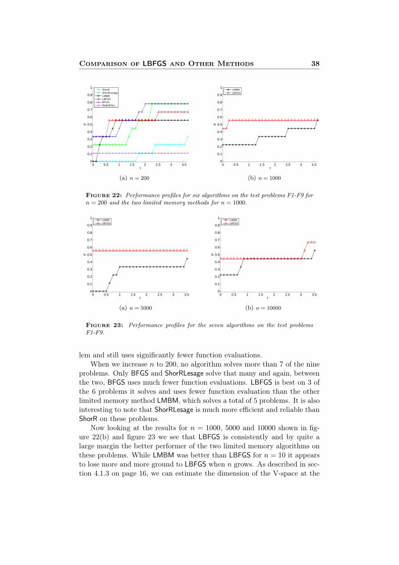
Figure 22: Performance profiles for six algorithms on the test problems F1-F9 forn = 200 and the two limited memory methods for n = 1000.
0 0.5 1 1.5 2 2.5 3 3.50
0.1
0.2
0.3
0.4
0.5
0.6
0.7
0.8
0.9
1
τ
ρ
LMBMLBFGS
(a) n = 5000
0 0.5 1 1.5 2 2.5 3 3.50
0.1
0.2
0.3
0.4
0.5
0.6
0.7
0.8
0.9
1
τ
ρ
LMBMLBFGS
(b) n = 10000
Figure 23: Performance profiles for the seven algorithms on the test problemsF1-F9.
lem and still uses significantly fewer function evaluations.When we increase n to 200, no algorithm solves more than 7 of the nine
problems. Only BFGS and ShorRLesage solve that many and again, betweenthe two, BFGS uses much fewer function evaluations. LBFGS is best on 3 ofthe 6 problems it solves and uses fewer function evaluation than the otherlimited memory method LMBM, which solves a total of 5 problems. It is alsointeresting to note that ShorRLesage is much more efficient and reliable thanShorR on these problems.
Now looking at the results for n = 1000, 5000 and 10000 shown in fig-ure 22(b) and figure 23 we see that LBFGS is consistently and by quite alarge margin the better performer of the two limited memory algorithms onthese problems. While LMBM was better than LBFGS for n = 10 it appearsto lose more and more ground to LBFGS when n grows. As described in sec-tion 4.1.3 on page 16, we can estimate the dimension of the V-space at the
Comparison of LBFGS and Other Methods 39
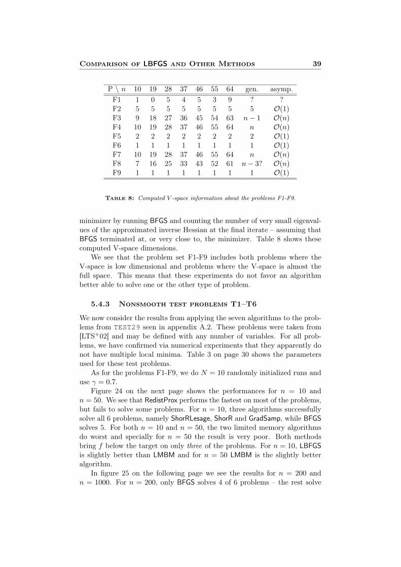
P \ n 10 19 28 37 46 55 64 gen. asymp.F1 1 0 5 4 5 3 9 ? ?F2 5 5 5 5 5 5 5 5 O(1)F3 9 18 27 36 45 54 63 n− 1 O(n)F4 10 19 28 37 46 55 64 n O(n)F5 2 2 2 2 2 2 2 2 O(1)F6 1 1 1 1 1 1 1 1 O(1)F7 10 19 28 37 46 55 64 n O(n)F8 7 16 25 33 43 52 61 n− 3? O(n)F9 1 1 1 1 1 1 1 1 O(1)
Table 8: Computed V -space information about the problems F1-F9.
minimizer by running BFGS and counting the number of very small eigenval-ues of the approximated inverse Hessian at the final iterate – assuming thatBFGS terminated at, or very close to, the minimizer. Table 8 shows thesecomputed V-space dimensions.
We see that the problem set F1-F9 includes both problems where theV-space is low dimensional and problems where the V-space is almost thefull space. This means that these experiments do not favor an algorithmbetter able to solve one or the other type of problem.
5.4.3 Nonsmooth test problems T1–T6
We now consider the results from applying the seven algorithms to the prob-lems from TEST29 seen in appendix A.2. These problems were taken from[LTS+02] and may be defined with any number of variables. For all prob-lems, we have confirmed via numerical experiments that they apparently donot have multiple local minima. Table 3 on page 30 shows the parametersused for these test problems.
As for the problems F1-F9, we do N = 10 randomly initialized runs anduse γ = 0.7.
Figure 24 on the next page shows the performances for n = 10 andn = 50. We see that RedistProx performs the fastest on most of the problems,but fails to solve some problems. For n = 10, three algorithms successfullysolve all 6 problems, namely ShorRLesage, ShorR and GradSamp, while BFGSsolves 5. For both n = 10 and n = 50, the two limited memory algorithmsdo worst and specially for n = 50 the result is very poor. Both methodsbring f below the target on only three of the problems. For n = 10, LBFGSis slightly better than LMBM and for n = 50 LMBM is the slightly betteralgorithm.
In figure 25 on the following page we see the results for n = 200 andn = 1000. For n = 200, only BFGS solves 4 of 6 problems – the rest solve

Comparison of LBFGS and Other Methods 40
0 0.5 1 1.5 2 2.5 3 3.50
0.1
0.2
0.3
0.4
0.5
0.6
0.7
0.8
0.9
1
τ
ρ
ShorRShorRLesageLMBMLBFGSBFGSGradSampRedistProx
(a) n = 10
0 0.5 1 1.5 2 2.5 3 3.50
0.1
0.2
0.3
0.4
0.5
0.6
0.7
0.8
0.9
1
τ
ρ
ShorRShorRLesageLMBMLBFGSBFGSRedistProx
(b) n = 50
Figure 24: Performance profiles for the seven algorithms on the test problemsT1-T6.
either 3 or 2 problems. On this problem set, RedistProx does much betterthan that of section 5.4.2. Although it is still not very robust, it uses veryfew function evaluations to solve the problems that it successfully solves.
When n = 1000, only the two limited memory algorithms are feasible touse and we see from figure 25(b) that both algorithms succeed on 3 of the 6problems. LBFGS is best on two of them and LMBM on the last.
It is clear from these experiments that the problems T1-T6 are generallyharder than the problems F1-F9 for which we presented results in section5.4.2. In table 9 on the next page, we see the V -space information that BFGSwas able to provide for the problems T1-T6. We see that as for the problemsF1-F9, we have also in this problem set problems of both high and low V -space dimension – it was, however, much more difficult to determine howmany eigenvalues of the inverse Hessian were bounded away from zero. To
0 0.5 1 1.5 2 2.5 3 3.50
0.1
0.2
0.3
0.4
0.5
0.6
0.7
0.8
0.9
1
τ
ρ
ShorRShorRLesageLMBMLBFGSBFGSRedistProx
(a) n = 200
0 0.5 1 1.5 2 2.5 30
0.1
0.2
0.3
0.4
0.5
0.6
0.7
0.8
0.9
1
τ
ρ
LMBMLBFGS
(b) n = 1000
Figure 25: Performance profiles for six algorithms on the test problems T1-T6 forn = 200 and the two limited memory methods for n = 1000.

Comparison of LBFGS and Other Methods 41
P \ n 10 20 30 40 50 60 70 gen. asymp.T1 10 20 30 40 50 60 70 n O(n)T2 4 5 6 7 7? 7? 8? ? O(1)?T3 1 1 1 1 1 1 1 1 O(1)T4 8 18 28 38 49(!) 58 68 n− 2? O(n)T5 10 20 30 40 50 60 70 n O(n)T6 10 20 30 40 50 60 70 n O(n)
Table 9: Computed V -space information about the problems T1-T6. A question-mark indicates that BFGS was unable to solve the problem to an accuracy sufficientto display any useful V -space information.
0 5 10 15 20 2510
−18
10−16
10−14
10−12
10−10
10−8
10−6
10−4
10−2
100
(a) T3
0 100 200 300 400 500 600 70010
−18
10−16
10−14
10−12
10−10
10−8
10−6
10−4
10−2
100
102
(b) T4
0 100 200 300 400 500 600 700 800 90010
−14
10−12
10−10
10−8
10−6
10−4
10−2
100
102
104
106
(c) T2
Figure 26: Eigenvalues of Cj as function of iteration counter j for selected prob-lems from the problem set T1-T6 with n = 60.
see the difficulty, consider the plots in figure 26. In the left and the middlepane of figure 26 it is not hard to see that the eigenvalues separate in twogroups: those that go to zero and those that do not. In fact we can countthat for (a) T3, one eigenvalue goes to zero (b) T4, all but two eigenvaluesgo to zero. As seen in the right pane, it is essentially not possible for (c) T2to determine how many eigenvalues go to zero before BFGS terminates.
For the problems F1-F9 from section 5.4.2, we were able to compare thetwo limited memory algorithms when n = 5000 and n = 10000. For theproblem set T1-T6, however, neither method succeeds in enough cases tomake comparison meaningful.
5.4.4 Nonconvex problems with several local minima
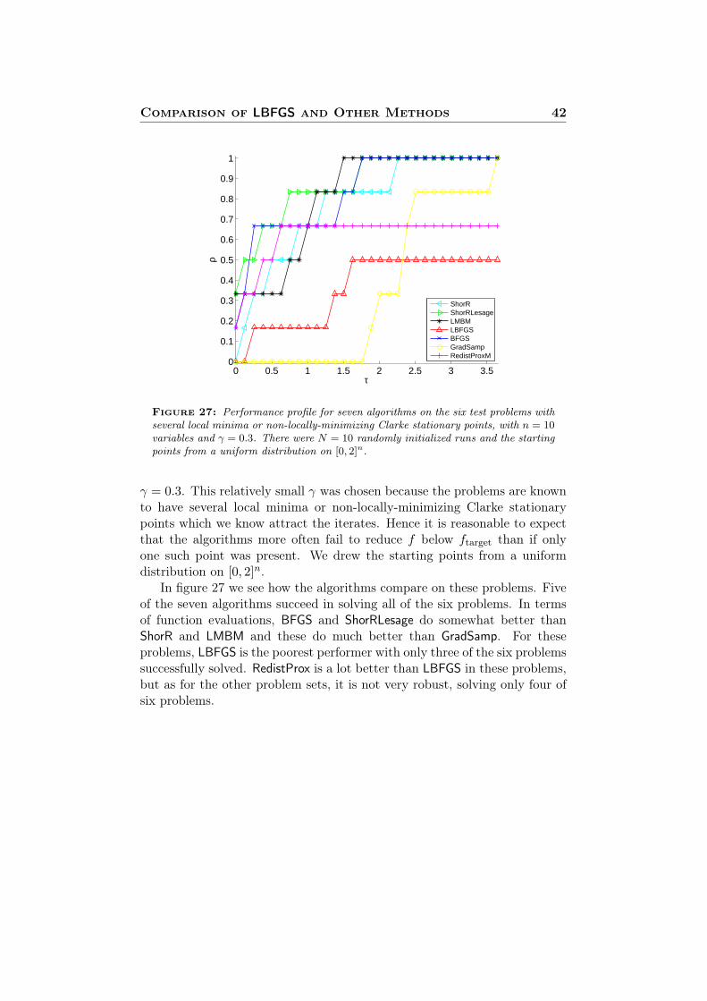
In this section, we present results from comparing the seven algorithms onproblems that have several local minima or non-locally-minimizing Clarkestationary points. These problems are the three problems P1-P3 shownin appendix A.3 along with the nonsmooth Rosenbrock function of Section4.2.4, the Nesterov problem of 4.2.5 and the Schatten norm problem of sec-tion 5.3.3 but here all with n = 10 variables.
For these problems we do N = 10 randomly initialized runs and set
Comparison of LBFGS and Other Methods 42
0 0.5 1 1.5 2 2.5 3 3.50
0.1
0.2
0.3
0.4
0.5
0.6
0.7
0.8
0.9
1
τ
ρ
ShorRShorRLesageLMBMLBFGSBFGSGradSampRedistProxM
Figure 27: Performance profile for seven algorithms on the six test problems withseveral local minima or non-locally-minimizing Clarke stationary points, with n = 10variables and γ = 0.3. There were N = 10 randomly initialized runs and the startingpoints from a uniform distribution on [0, 2]n.
γ = 0.3. This relatively small γ was chosen because the problems are knownto have several local minima or non-locally-minimizing Clarke stationarypoints which we know attract the iterates. Hence it is reasonable to expectthat the algorithms more often fail to reduce f below ftarget than if onlyone such point was present. We drew the starting points from a uniformdistribution on [0, 2]n.
In figure 27 we see how the algorithms compare on these problems. Fiveof the seven algorithms succeed in solving all of the six problems. In termsof function evaluations, BFGS and ShorRLesage do somewhat better thanShorR and LMBM and these do much better than GradSamp. For theseproblems, LBFGS is the poorest performer with only three of the six problemssuccessfully solved. RedistProx is a lot better than LBFGS in these problems,but as for the other problem sets, it is not very robust, solving only four ofsix problems.

Comparison of LBFGS and Other Methods 43
5.5 Summary of Observations
In the previous sections we have found that for
• small- and medium-scale problems (1 ≤ n < 1000),
– BFGS was, together with ShorRLesage, generally the most robustalgorithm solving totally 45 of 51 problems. In terms of functionevaluations, it was the best algorithm on the problems F1-F9 forn = 10, 50 and 200. It was also the most efficient on the eigenvalueproblem (5.1) and the Schatten norm problem (5.3). It should alsobe noted for its robustness and its consistent convergence rates,see figures in section 4.2.
– ShorRLesage was equally robust solving totally 47 of 51 problems.In terms of function evaluations, it was rarely the most efficientexcept on the small scale versions of the problems T1-T6 and thecondition number problem (5.2). It used more function evalu-ations than BFGS on the problems F1-F9 but on the problemsT1-T6 it was slightly more robust than BFGS.
– ShorR was satisfactory only for the very small scale versions of theproblems T1-T6 and only in terms of robustness. Its performancedropped dramatically for larger n. With a few exceptions, ShorRappeared to be worse than ShorRLesage, so there is no reason toprefer it.
– RedistProx was generally the least predictable of the tested algo-rithms. It was unable to solve any of the matrix problems and didnot compare very well on the performance profiles for the prob-lem set F1-F9 – except when n = 10, where it used few functionevaluations but failed to solve two of the problems. It was overallnot very robust, failing on seven of nine the problems for n = 50and eight of nine for n = 200. On the problem set T1-T6, itfailed on two of the six problems for n = 10 and on three of sixfor n = 50. On the other hand, in the same problem set, it wasbest on almost all of the problems that it successfully solved. Onthe nonconvex problems of section 5.4.4, it was about as fast asthe best methods on this set, but failed on two of six problems.
– LBFGS was, on the small- and medium-scale problems, compa-rable to LMBM. It was more efficient on the condition numberproblem (5.2), but clearly worse on the Schatten norm problem(5.3). On the eigenvalue problem (5.1), it was more robust thanLMBM. On the problems F1-F9, LBFGS was overall marginallybetter than LMBM for n ≤ 200. On the problems T1-T6, LBFGSwas best for smaller n, but the two were about equal for largern. Generally the behavior of LBFGS is much more erratic than

Comparison of LBFGS and Other Methods 44
that of BFGS. This was particularly clear on the problems of sec-tion 4.2. LBFGS did very poorly on the nonconvex problems ofsection 5.4.4. Here it solved only three of six problems and it didso using significantly more function evaluations than every otheralgorithm except GradSamp.
– LMBM was similar in its behavior to LBFGS on most small-scaleproblems. The only exception was the nonconvex problems of sec-tion 5.4.4. Here LMBM did well solving all problems with aboutthe same use of function evaluations as the other successful algo-rithms.
– GradSamp was included only in the performance profiles for n =10. The reason for this was its intense use of function evaluations.It was simply infeasible to solve bigger problems. However, itshould be noted that it was very robust, solving all problems onwhich it was applied. Its need for function evaluations was fargreater than that of any other method.
• large-scale problems (n ≥ 1000),
– LBFGS was notably superior to LMBM. On the test problems F1-F9, LBFGS got relatively better compared to LMBM when n wasbigger. For n = 1000, both methods solved five of nine prob-lems and LBFGS was best on all but one of them. For n = 5000,LBFGS again solved five while LMBM solved four of nine prob-lems and LBFGS was best on all of them. Similarly, LBFGS wassuperior for n = 10000. On the problem set T1-T6, which wasoverall a harder set of problems than F1-F9, LBFGS and LMBMboth successfully solved three problems for n = 1000 and LBFGSwas more efficient on two of them. However, neither method suc-ceeded when n = 5000 or n = 10000. Overall, LBFGS was clearlysuperior to LMBM for large n, which is a surprising conclusion,considering that LMBM was specifically designed for large-scalenonsmooth optimization while LBFGS was originally meant forsmooth problems.
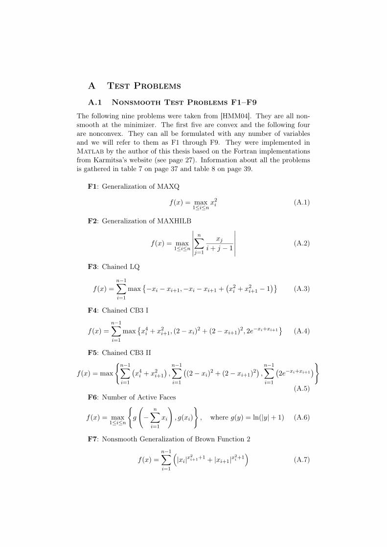
A Test Problems
A.1 Nonsmooth Test Problems F1–F9
The following nine problems were taken from [HMM04]. They are all non-smooth at the minimizer. The first five are convex and the following fourare nonconvex. They can all be formulated with any number of variablesand we will refer to them as F1 through F9. They were implemented inMatlab by the author of this thesis based on the Fortran implementationsfrom Karmitsa’s website (see page 27). Information about all the problemsis gathered in table 7 on page 37 and table 8 on page 39.
F1: Generalization of MAXQ
f(x) = max1≤i≤n
x2i (A.1)
F2: Generalization of MAXHILB
f(x) = max1≤i≤n
∣∣∣∣∣∣n∑j=1
xji+ j − 1
∣∣∣∣∣∣ (A.2)
F3: Chained LQ
f(x) =n−1∑i=1
max{−xi − xi+1,−xi − xi+1 +
(x2i + x2
i+1 − 1)}
(A.3)
F4: Chained CB3 I
f(x) =n−1∑i=1
max{x4i + x2
i+1, (2− xi)2 + (2− xi+1)2, 2e−xi+xi+1}
(A.4)
F5: Chained CB3 II
f(x) = max
{n−1∑i=1
(x4i + x2
i+1
),n−1∑i=1
((2− xi)2 + (2− xi+1)2
),n−1∑i=1
(2e−xi+xi+1
)}(A.5)
F6: Number of Active Faces
f(x) = max1≤i≤n
{g
(−
n∑i=1
xi
), g(xi)
}, where g(y) = ln(|y|+ 1) (A.6)
F7: Nonsmooth Generalization of Brown Function 2
f(x) =n−1∑i=1
(|xi|x
2i+1+1 + |xi+1|x
2i +1)
(A.7)
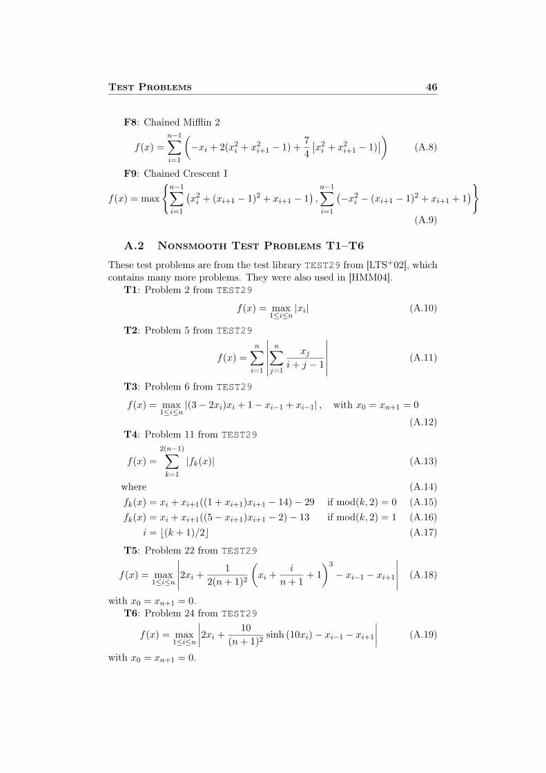
Test Problems 46
F8: Chained Mifflin 2
f(x) =n−1∑i=1
(−xi + 2(x2
i + x2i+1 − 1) +
74
∣∣x2i + x2
i+1 − 1)∣∣) (A.8)
F9: Chained Crescent I
f(x) = max
{n−1∑i=1
(x2i + (xi+1 − 1)2 + xi+1 − 1
),n−1∑i=1
(−x2
i − (xi+1 − 1)2 + xi+1 + 1)}
(A.9)
A.2 Nonsmooth Test Problems T1–T6
These test problems are from the test library TEST29 from [LTS+02], whichcontains many more problems. They were also used in [HMM04].
T1: Problem 2 from TEST29
f(x) = max1≤i≤n
|xi| (A.10)
T2: Problem 5 from TEST29
f(x) =n∑i=1
∣∣∣∣∣∣n∑j=1
xji+ j − 1
∣∣∣∣∣∣ (A.11)
T3: Problem 6 from TEST29
f(x) = max1≤i≤n
|(3− 2xi)xi + 1− xi−1 + xi−1| , with x0 = xn+1 = 0
(A.12)T4: Problem 11 from TEST29
f(x) =2(n−1)∑k=1
|fk(x)| (A.13)
where (A.14)fk(x) = xi + xi+1((1 + xi+1)xi+1 − 14)− 29 if mod(k, 2) = 0 (A.15)fk(x) = xi + xi+1((5− xi+1)xi+1 − 2)− 13 if mod(k, 2) = 1 (A.16)
i = b(k + 1)/2c (A.17)
T5: Problem 22 from TEST29
f(x) = max1≤i≤n
∣∣∣∣∣2xi + 12(n+ 1)2
(xi +
i
n+ 1+ 1)3
− xi−1 − xi+1
∣∣∣∣∣ (A.18)
with x0 = xn+1 = 0.T6: Problem 24 from TEST29
f(x) = max1≤i≤n
∣∣∣∣2xi + 10(n+ 1)2
sinh (10xi)− xi−1 − xi+1
∣∣∣∣ (A.19)
with x0 = xn+1 = 0.
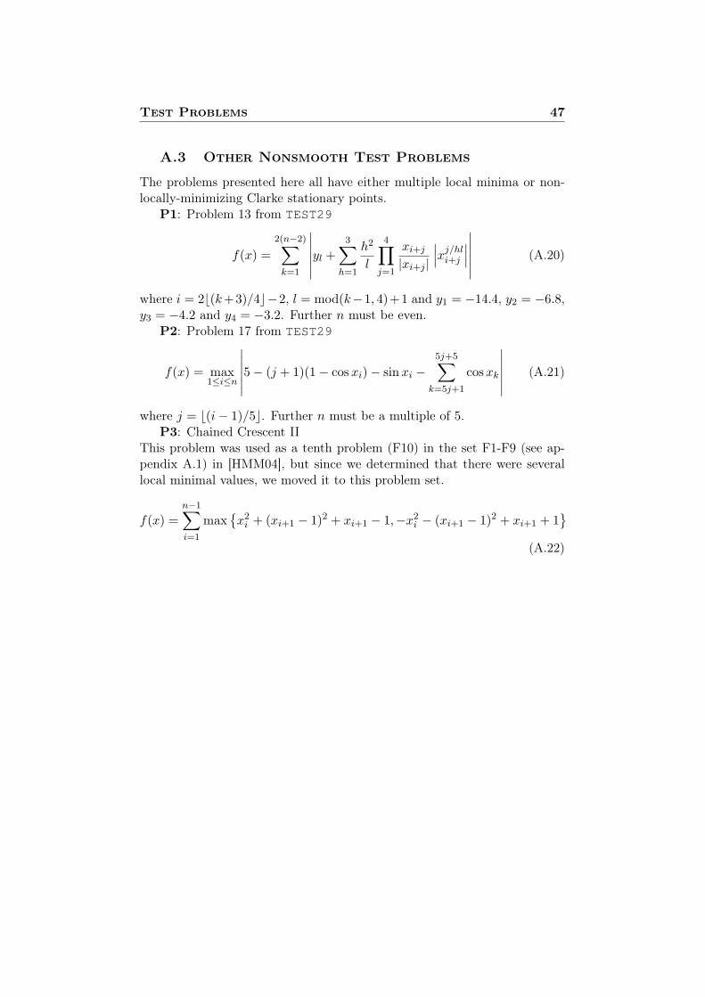
Test Problems 47
A.3 Other Nonsmooth Test Problems
The problems presented here all have either multiple local minima or non-locally-minimizing Clarke stationary points.
P1: Problem 13 from TEST29
f(x) =2(n−2)∑k=1
∣∣∣∣∣∣yl +3∑
h=1
h2
l
4∏j=1
xi+j|xi+j |
∣∣∣xj/hli+j
∣∣∣∣∣∣∣∣∣ (A.20)
where i = 2b(k+3)/4c−2, l = mod(k−1, 4)+1 and y1 = −14.4, y2 = −6.8,y3 = −4.2 and y4 = −3.2. Further n must be even.
P2: Problem 17 from TEST29
f(x) = max1≤i≤n
∣∣∣∣∣∣5− (j + 1)(1− cosxi)− sinxi −5j+5∑
k=5j+1
cosxk
∣∣∣∣∣∣ (A.21)
where j = b(i− 1)/5c. Further n must be a multiple of 5.P3: Chained Crescent II
This problem was used as a tenth problem (F10) in the set F1-F9 (see ap-pendix A.1) in [HMM04], but since we determined that there were severallocal minimal values, we moved it to this problem set.
f(x) =n−1∑i=1
max{x2i + (xi+1 − 1)2 + xi+1 − 1,−x2
i − (xi+1 − 1)2 + xi+1 + 1}
(A.22)
REFERENCES 48
References
[BL00] J. Borwein and A. S. Lewis. Convex Analysis and Nonlinear Op-timization: Theory and Examples. Springer, 2000.
[BLO02] J. V. Burke, A. S. Lewis, and M. L. Overton. Two numericalmethods for optimizing matrix stability. Linear Algebra Appl.,351-352:117–145, 2002.
[BLO05] J. V. Burke, A. S. Lewis, and M. L. Overton. A robust gradientsampling algorithm for nonsmooth, nonconvex optimization. SIAMJ. Optimization, 15:751–779, 2005.
[BLO08] J. V. Burke, A. S. Lewis, and M. L. Overton. The speed of Shor’sR-algorithm. IMA J. Numer. Anal., 28(4):711–720, 2008.
[Bro70] C. G. Broyden. The convergence of a class of double-rank mini-mization algorithms. Journal of the Institute of Mathematics andIts Applications, 6(1):76–90, 1970.
[BV04] Stephen Boyd and Lieven Vandenberghe. Convex Optimization.Cambridge University Press, 2004.
[Cla83] F. H. Clarke. Optimization and Nonsmooth Analysis. John Wiley,New York. Reprinted by SIAM, Philadelphia, 1983.
[CR08] E. J. Candès and B. Recht. Exact matrix completion via convexoptimization. Found. of Comput. Math., 9:717–772, 2008.
[DM02] E.D. Dolan and J.J. More. Benchmarking optimization softwarewith performance profiles. Mathematical Programming, 91(2):201–213, 2002.
[Fle70] R. Fletcher. A new approach to variable metric algorithms. Com-puter Journal, 13(3):317–322, 1970.
[Gol70] D. Goldfarb. A family of variable metric updates derived by varia-tional means. Mathematics of Computation, 24(109):23–26, 1970.
[Gur09] M. Gurbuzbalaban, 2009. Private communication.
[GV06] C. Greif and J. Varah. Minimizing the condition number for smallrank modifications. SIAM J. Matrix Anal. Appl., 29(1):82–97,2006.
[HMM04] M. Haarala, K. Miettinen, and M. M. Makela. New limited mem-ory bundle method for large-scale nonsmooth optimization. Opti-mization Methods and Software, 19(6):673–692, 2004.

REFERENCES 49
[HS09] W. Hare and C Sagastizabal. A redistributed proximal bundlemethod for nonconvex optimization. submitted to SIAM J. Opt,2009.
[HUL93] J.B. Hiriart-Urruty and C. Lemaréchal. Convex Analysis and Min-imization Algorithms. Springer Verlag, 1993.
[Kiw85] K.C. Kiwiel. Methods of Descent for Nondifferentiable Optimiza-tion. Lecture Notes in Mathematics 1133. Springer Verlag, 1985.
[Kiw07] K.C. Kiwiel. Convergence of the gradient sampling algorithm fornonsmooth nonconvex optimization. SIAM Journal on Optimiza-tion, 18(2):379–388, 2007.
[KK00] F. Kappel and A. Kuntsevich. An implementation of Shor’s R-algorithm. Computational Optimization and Applications, 15:193–205, 2000.
[Lem81] C. Lemaréchal. A view of line searches. Optimization and OptimalControl, Auslender, Oettli, Stoer Eds, Lecture Notes in Controland Information Sciences 30, pages 59–78, 1981.
[Lew02] A. S. Lewis. Active sets, nonsmoothness, and sensitivity. SIAM J.on Optimization, 13(3):702–725, 2002.
[LO10] A.S. Lewis and M.L. Overton. Nonsmooth optimization via BFGS.Submitted to SIAM J. Optimization, 2010.
[LOS00] C. Lemaréchal, F. Oustry, and C. Sagastizábal. The U-Lagrangianof a convex function. Trans. Amer. Math. Soc., 352:711.729, 2000.
[LTS+02] L. Lukšan, M. Tuma, M. Siska, J. Vlček, and N. Ramesova. UFO2002. Interactive system for universal functional optimization. Re-search report, Academy of Sciences of the Czech Republic, 2002.
[LV97] L. Lukšan and J. Vlček. PBUN, PNEW - a bundle-type algorithmsfor nonsmooth optimization. Research report, Academy of Sciencesof the Czech Republic, 1997.
[LV99] L. Lukšan and J. Vlček. Globally convergent variable metric meth-ods for convex nonsmooth unconstrained minimization. Journal ofOptimization Theory and Applications, 102(3):593–613, 1999.
[MOS03] MOSEK. Mosek optimization software, 2003. http://www.mosek.com/.
[MY09] Pierre Maréchal and Jane J. Ye. Optimizing condition numbers.SIAM J. Optim., 20(2):935–947, 2009.
REFERENCES 50
[Noc80] J. Nocedal. Updating quasi-Newton matrices with limited storage.Mathematics of Computation, 35(151):773–782, 1980.
[NW06] J. Nocedal and S. Wright. Numerical Optimization. Springer, 2ndedition, 2006.
[RW98] R.T. Rockafellar and R.J.B. Wets. Variational Analysis. Springer,New York, 1998.
[Sha70] D. F. Shanno. Conditioning of quasi-Newton methods for func-tion minimization. Mathematics of Computation, 24(111):647–656,1970.
[Sho85] N. Z. Shor. Minimization Methods for Non-Differentiable Func-tions. Springer Verlag, 1985.


![A BFGS-SQP method for nonsmooth, nonconvex, constrained ...coral.ise.lehigh.edu/frankecurtis/files/papers/CurtMitcOver17.pdf · for a proton exchange membrane fuel cell system [48],](https://img.pdfslide.net/doc/110x75/5e486980acce3e7a4d4f035c/a-bfgs-sqp-method-for-nonsmooth-nonconvex-constrained-coralise-for-a-proton.jpg)