Nonsmooth Analysis and Optimization

NONSMOOTH ANALYSIS AND

OPTIMIZATION

lecture notes

Christian Clason

March 6, 2018

[email protected]

hps://udue.de/clason

mailto:[email protected]

https://udue.de/clason

CONTENTS

introduction 1

I BACKGROUND

1 functional analysis 4

1.1 Normed vector spaces 4

1.2 Strong and weak convergence 6

1.3 Hilbert spaces 12

2 calculus of variations 13

2.1 The direct method 13

2.2 Dierential calculus in Banach spaces 17

2.3 Superposition operators 20

II CONVEX ANALYSIS

3 convex functions 24

4 convex subdifferentials 33

5 fenchel duality 44

6 monotone operators and proximal points 51

6.1 Monotone operators 51

6.2 Resolvents and proximal points 55

6.3 Moreau–Yosida regularization 61

7 proximal point and splitting methods 67

7.1 Proximal point method 67

7.2 Explicit spliing 69

7.3 Implicit spliing 73

7.4 Primal-dual extragradient method 74

i

contents

III LIPSCHITZ ANALYSIS

8 clarke subdifferentials 79

9 semismooth newton methods 92

ii

INTRODUCTION

Optimization is concerned with nding solutions to problems of the form

min

x∈UF (x)

for a function F : X → R and a set U ⊂ X . Specically, one considers the following

questions:

1. Does this problem admit a solution, i.e., is there an x ∈ U such that

F (x) ≤ F (x) for all x ∈ U ?

2. Is there an intrinsic characterization of x , i.e., one not requiring comparison with all

other x ∈ U ?

3. How can this x be computed (eciently)?

For U ⊂ Rn, these questions can be answered roughly as follows.

1. IfU is compact and F is continuous, the Weierstraß Theorem yields that F attains its

minimum at a point x ∈ U (as well as its maximum).

2. If F is dierentiable, the Fermat principle

0 = F ′(x)

holds.

3. If F is continuously dierentiable and U is open, one can apply the steepest descentor gradient method to compute an x satisfying the Fermat principle: Choosing a

starting point x0and setting

xk+1 = xk − tkF′(xk), k = 0, . . . ,

for suitable step sizes tk , we have that xk → x for k →∞.

If F is even twice continuously dierentiable, one can apply Newton’s method to the

Fermat principle: Choosing a suitable starting point x0and setting

xk+1 = xk − F ′′(xk)−1F ′(xk), k = 0, . . . ,

we have that xk → x for k →∞.

1

introduction

However, there are many practically relevant functions that are not dierentiable, such

as the absolute value or maximum function. The aim of nonsmooth analysis is therefore

to nd generalized derivative concepts that on the one hand allow the above sketched

approach for such functions and on the other hand admit a suciently rich calculus to

give explicit derivatives for a suciently large class of functions. Here we concentrate on

the two classes of

i) convex functions,

ii) locally Lipschitz continuous functions,

which together cover a wide spectrum of applications. In particular, the rst class will lead

us to generalized gradient methods, while the second class are the basis for generalized

Newton methods. To x ideas, we aim at treating problems of the form

min

x∈C

1

p‖F (x) − z‖

pY +

α

q‖x ‖

qX

for a convex set C ⊂ X , a (possibly nonlinear but dierentiable) operator F : X → Y ,

α ≥ 0 and p,q ∈ [1,∞) (in particular, p = 1 and/or q = 1). Such problems are ubiquitous

in inverse problems, imaging, and optimal control of dierential equations. Hence, we

consider optimization in innite-dimensional function spaces; i.e., we are looking for

functions as minimizers. The main benet (beyond the frequently cleaner notation) is that

the developed algorithms become discretization independent: they can be applied to any

(reasonable) nite-dimensional approximation, and the details – in particular, the neness

– of the approximation do not inuence the convergence behavior of the algorithm.

Since we deal with innite-dimensional spaces, some knowledge of functional analysis is

assumed, but the necessary background will be summarized in Chapter 1. The results on

pointwise operators on Lebesgue spaces also require elementary (Lebesgue) measure and

integration theory. Basic familiarity with classical nonlinear optimization is helpful but

not necessary.

These notes are based on graduate lectures given 2014 (in slightly dierent form) and

2016–2017 at the University of Duisburg-Essen; parts were also taught at the Winter School

“Modern Methods in Nonsmooth Optimization” organized by Christian Kanzow and Daniel

Wachsmuth at the University Würzburg in February 2018. As such, no claim is made of

originality (beyond possibly the selection – and, more importantly, omission – of material).

Rather, like a magpie, I have collected the shiniest results and proofs I could nd, mainly

from [Brokate 2014; Schirotzek 2007; Attouch, Buttazzo, et al. 2006; Bauschke & Combettes

2017; Clarke 2013; Ulbrich 2002; Schiela 2008]. All mistakes, of course, are entirely my

own.

2

Part I

BACKGROUND

3

1 FUNCTIONAL ANALYSIS

In this chapter we collect the basic concepts and results (and, more importantly, x notations)

from linear functional analysis that will be used in the following. For details and proofs,

the reader is referred to the standard literature, e.g., [Alt 2016; Brezis 2010].

1.1 normed vector spaces

In the following, X will denote a vector space over the eld K, where we restrict ourselves

for the sake of simplicity to the case K = R. A mapping ‖ · ‖ : X → R+ := [0,∞) is called

a norm (on X ), if for all x ∈ X there holds

(i) ‖λx ‖ = |λ |‖x ‖ for all λ ∈ K,

(ii) ‖x + y ‖ ≤ ‖x ‖ + ‖y ‖ for all y ∈ X ,

(iii) ‖x ‖ = 0 if and only if x = 0 ∈ X .

Example 1.1. (i) The following mappings dene norms on X = RN:

‖x ‖p =

(N∑i=1

|xi |p

)1/p

1 ≤ p < ∞,

‖x ‖∞ = max

i=1,...,N|xi |.

(ii) The following mappings dene norms on X = `p (the space of real-valued

sequences for which these terms are nite):

‖x ‖p =

(∞∑i=1

|xi |p

)1/p

1 ≤ p < ∞,

‖x ‖∞ = sup

i=1,...,∞|xi |.

(iii) The following mappings dene norms on X = Lp(Ω) (the space of real-valued

4

1 functional analysis

measurable functions on the domain Ω ⊂ Rnfor which these terms are nite):

‖u‖p =

(∫Ω|u(x)|p

)1/p

1 ≤ p < ∞,

‖u‖∞ = ess sup

x∈Ω|u(x)|.

(iv) The following mapping denes a norm on X = C(Ω) (the space of continuous

functions on Ω):

‖u‖C = sup

x∈Ω

|u(x)|.

An analogous norm is dened on X = C0(Ω) (the space of continuous functions

on Ω with compact support), if the supremum is taken only over the space of

continuous functions on Ω with compact support), if the supremum is taken

only over x ∈ Ω.

If ‖ · ‖ is a norm on X , the tuple (X , ‖ · ‖) is called a normed vector space, and one frequently

denotes this by writing ‖ · ‖X . If the norm is canonical (as in Example 1.1 (ii)–(iv)), it is often

omitted and one speaks simply of “the normed vector space X ”.

Two norms ‖ · ‖1, ‖ · ‖2 are called equivalent on X , if there are constants c1, c2 > 0 such

that

c1‖x ‖2 ≤ ‖x ‖1 ≤ c2‖x ‖2 for all x ∈ X .

If X is nite-dimensional, all norms on X are equivalent. However, the corresponding con-

stants c1 and c2 may depend on the dimension N of X ; avoiding such dimension-dependent

constants is one of the main reasons to consider optimization in innite-dimensional

spaces.

If (X , ‖ · ‖X ) and (Y , ‖ · ‖Y ) are normed vector spaces with X ⊂ Y , we call X continuouslyembedded in Y , denoted by X → Y , if there exists a C > 0 with

‖x ‖Y ≤ C‖x ‖X for all x ∈ X .

We now consider mappings between normed vector spaces. In the following, let (X , ‖ · ‖X )and (Y , ‖ · ‖Y ) be normed vector spaces, U ⊂ X , and F : U → Y be a mapping. We denote

by

• dom F := U the domain of denition of F ;

• ker F := x ∈ U : F (x) = 0 kernel or null space of F ;

• ran F := F (x) ∈ Y : x ∈ U the range of F ;

• graph F := (x ,y) ∈ X × Y : y = F (x) the graph of F .

5


We call F : U → Y

• continuous in x ∈ U , if for all ε > 0 there exists a δ > 0 with

‖F (x) − F (z)‖Y ≤ ε for all z ∈ U with ‖x − z‖X ≤ δ ;

• Lipschitz continuous, if there exists an L > 0 (called Lipschitz constant) with

‖F (x1) − F (x2)‖Y ≤ L‖x1 − x2‖X for all x1,x2 ∈ U .

• locally Lipschitz continuous in x ∈ U , if there exists a δ > 0 and a L = L(x ,δ ) > 0

with

‖F (x) − F (z)‖Y ≤ L‖x − z‖X for all z ∈ U with ‖x − z‖X ≤ δ .

If T : X → Y is linear, continuity is equivalent to the existence of a constant C > 0 with

‖Tx ‖Y ≤ C‖x ‖X for all x ∈ X .

For this reason, continuous linear mappings are called bounded; one speaks of a bounded

linear operator. The space L(X ,Y ) of bounded linear operators is itself a normed vector

space if endowed with the operator norm

‖T ‖L(X ,Y ) = sup

x∈X\0

‖Tx ‖Y‖x ‖X

= sup

‖x ‖X=1

‖Tx ‖Y = sup

‖x ‖X ≤1

‖Tx ‖Y

(which is equal to the smallest possible constant C in the denition of continuity). If

T ∈ L(X ,Y ) is bijective, the inverse T −1: Y → X is continuous if and only if there exists a

c > 0 with

c‖x ‖X ≤ ‖Tx ‖Y for all x ∈ X .

In this case, ‖T −1‖L(Y ,X ) = c−1

for the largest possible choice of c .

1.2 strong and weak convergence

A norm directly induces a notion of convergence, the so-called strong convergence: A

sequence xnn∈N ⊂ X converges (strongly in X ) to a x ∈ X , denoted by xn → x , if

lim

n→∞‖xn − x ‖X = 0.

A subset U ⊂ X is called

• closed, if for every convergent sequence xnn∈N ⊂ U the limit x ∈ U as well;

6


• compact, if every sequence xnn∈N ⊂ U contains a convergent subsequence xnk k∈Nwith limit x ∈ U .

A mapping F : X → Y is continuous if and only if xn → x implies F (xn) → F (x), and closed,

if xn → x and F (xn) → y imply F (x) = y (i.e., graph F ⊂ X × Y is a closed set).

Further we dene for later use for x ∈ X and r > 0

• the open ball Or (x) := z ∈ X : ‖x − z‖X < r and

• the closed ball Kr (x) := z ∈ X : ‖x − z‖X ≤ r .

The closed ball around 0 ∈ X with radius 1 is also referred to a the unit ball BX . A set

U ⊂ X is called

• open, if for all x ∈ U there exists an r > 0 with Or (x) ⊂ U (i.e., all x ∈ U are interiorpoints of U , which together form the interior U o

);

• bounded, if it is contained in Kr (0) for a r > 0;

• convex, if for any x ,y ∈ U and λ ∈ [0, 1] also λx + (1 − λ)y ∈ U .

In normed vector spaces it always holds that the complement of an open set is closed and

vice versa (i.e., the closed sets in the sense of topology are exactly the (sequentially) closed

set as dened above). The denition of a norm directly implies that both open and closed

balls are convex.

A normed vector space X is called complete if every Cauchy sequence in X is convergent;

in this case,X is called a Banach space. All spaces in Example 1.1 are Banach spaces. If Y is a

Banach space, so is L(X ,Y ) if endowed with the operator norm. Convex subsets of Banach

spaces have the following useful property which derives from the Baire Theorem.

Lemma 1.2. Let X be a Banach space andU ⊂ X be closed and convex. Then

U o = x ∈ U : for all h ∈ X there is a δ > 0 with x + th ∈ U for all t ∈ [0,δ ] .

The set on the right-hand side is called algebraic interior or core. For this reason, Lemma 1.2

is sometimes referred to as the “core-int Lemma”. Note that the inclusion “⊂” always holds

in normed vector spaces due to the denition of interior points via open balls.

Of particular importance to us is the special case L(X ,Y ) for Y = R, the space of boundedlinear functionals on X . In this case, X ∗ := L(X ,R) is called the dual space (or just dual of

X . For x∗ ∈ X ∗ and x ∈ X , we set

〈x∗,x〉X := x∗(x) ∈ R.

This duality pairing indicates that we can also interpret it as x acting on x∗, which will

become important later. The denition of the operator norm immediately implies that

(1.1) 〈x∗,x〉X ≤ ‖x∗‖X ∗ ‖x ‖X for all x ∈ X ,x∗ ∈ X ∗.

7


In many cases, the dual of a Banach space can be identied with another known Banach

space.

Example 1.3. (i) (RN , ‖ · ‖p)∗ (RN , ‖ · ‖q)with p−1+q−1 = 1, where we set 0

−1 = ∞

and∞−1 = 0. The duality pairing is given by

〈x∗,x〉p =N∑i=1

x∗i xi .

(ii) (`p)∗ (`q) for 1 < p < ∞. The duality pairing is given by

〈x∗,x〉p =∞∑i=1

x∗i xi .

Furthermore, (`1)∗ = `∞, but (`∞)∗ is not a sequence space.

(iii) Analogously, Lp(Ω)∗ Lq(Ω) for 1 < p < ∞. The duality pairing is given by

〈u∗,u〉p =

∫Ωu∗(x)u(x)dx .

Furthermore, L1(Ω)∗ L∞(Ω), but L∞(Ω)∗ is not a function space.

(iv) C0(Ω)∗ M(Ω), the space of Radon measure; it contains among others the

Lebesgue measure as well as Dirac measuresδx forx ∈ Ω, dened viaδx (u) = u(x)for u ∈ C0(Ω). The duality pairing is given by

〈u∗,u〉C =

∫Ωu(x)du∗.

A central result on dual spaces is the Hahn–Banach Theorem, which comes in both an

algebraic and a geometric version.

Theorem 1.4 (Hahn–Banach, algebraic). Let X be a normed vector space. For any x ∈ X thereexists a x∗ ∈ X ∗ with

‖x∗‖X ∗ = 1 and 〈x∗,x〉X = ‖x ‖X .

Theorem 1.5 (Hahn–Banach, geometric). Let X be a normed vector space and A,B ⊂ X beconvex, nonempty, and disjoint.

(i) If A is open, there exists an x∗ ∈ X ∗ and a λ ∈ R with

〈x∗,x1〉X < λ ≤ 〈x∗,x2〉X for all x1 ∈ A,x2 ∈ B.

8


(ii) If A is closed and B is compact, there exists an x∗ ∈ X ∗ and a λ ∈ R with

〈x∗,x1〉X ≤ λ < 〈x∗,x2〉X for all x1 ∈ A,x2 ∈ B.

Particularly the geometric version – also referred to as separation theorems – is of crucial

importance in convex analysis. We will also require their following variant, which is known

as Eidelheit Theorem.

Corollary 1.6. Let X be a normed vector space and A,B ⊂ X be convex and nonempty. If theinterior Ao of A is nonempty and disjoint with B, there exists an x∗ ∈ X ∗ \ 0 and a λ ∈ Rwith

〈x∗,x1〉X ≤ λ ≤ 〈x∗,x2〉X for all x1 ∈ A,x2 ∈ B.

Proof. Theorem 1.5 (i) yields the existence of x∗ and λ satisfying the claim for all x1 ∈ Ao

(even with strict inequality, which also implies x∗ , 0). It thus remains to show that

〈x∗,x〉X ≤ λ also for x ∈ A \Ao. Since Ao

is nonempty, there exists an x0 ∈ Ao, i.e., there is

an r > 0 with Or (x0) ⊂ A. The convexity of A then implies that tx + (1 − t)x ∈ A for all

x ∈ Or (x0) and t ∈ [0, 1]. Hence,

tOr (x0) + (1 − t)x = Otr (tx0 + (1 − t)x) ⊂ A,

and in particular x(t) := tx0 + (1 − t)x ∈ Ao

for all t ∈ (0, 1).

We can thus nd a sequence xnn∈N ⊂ Ao(e.g., xn = x(n−1)) with xn → x . Due to the

continuity of x∗ ∈ X = L(X ,R) we can thus pass to the limit n →∞ and obtain

〈x∗,x〉X = lim

n→∞〈x∗,xn〉X ≤ λ.

In a certain way, a normed vector space is thus characterized by its dual. A direct conse-

quence of Theorem 1.4 is that the norm on a Banach space can be expressed in the manner

of an operator norm.

Corollary 1.7. Let X be a Banach space. Then for all x ∈ X ,

‖x ‖X = sup

‖x∗‖X ∗≤1

|〈x∗,x〉X |,

and the supremum is attained.

A vector x ∈ X can therefore be considered as a linear and, by (1.1), bounded functional on

X ∗, i.e., as an element of the bidual X ∗∗ := (X ∗)∗. The embedding X → X ∗∗ is realized by

the canonical injection

J : X → X ∗∗, 〈Jx ,x∗〉X ∗ := 〈x∗,x〉X for all x∗ ∈ X ∗.

9


Clearly, J is linear; Theorem 1.4 furthermore implies that ‖ Jx ‖X ∗∗ = ‖x ‖X . If the canonical

injection is surjective and we can thus identify X ∗∗ with X , the space X is called reexive.All nite-dimensional spaces are reexive, as are Example 1.1 (ii) and (iii) for 1 < p < ∞ but

not `1, `∞ as well as L1(Ω),L∞(Ω) and C(Ω).

The duality pairing induces further notions of convergence: the weak convergence on X as

well as the weak-∗ convergence on X ∗.

(i) A sequence xnn∈N ⊂ X converges weakly (in X ) to x ∈ X , denoted by xn x , if

〈x∗,xn〉X → 〈x∗,x〉X for all x∗ ∈ X ∗.

(ii) A sequence x∗nn∈N ⊂ X ∗ converges weakly-∗ (in X ∗) to x∗ ∈ X ∗, denoted by

x∗n ∗ x∗, if

〈x∗n,x〉X → 〈x∗,x〉X for all x ∈ X .

Weak convergence generalizes the concept of componentwise convergence in Rn, which –

as can be seen from the proof of the Heine–Borel Theorem – is the appropriate concept in

the context of compactness. Strong convergence implies weak convergence by continuity

of the duality pairing; in the same way, convergence with respect to the operator norm

(also called pointwise convergence) implies weak-∗ convergence. If X is reexive, weak

and weak-∗ convergence (both in X = X ∗∗!) coincide. In nite-dimensional spaces, all

convergence notions coincide.

If xn → x and x∗n ∗ x∗ or xn x and x∗n → x∗, then 〈x∗n,xn〉X → 〈x

∗,x〉X . However, the

duality pairing of weak(-∗) convergent sequences does not converge in general.

As for strong convergence, one denes weak(-∗) continuity and closedness of mappings

as well as weak(-∗) closedness and compactness of sets. The last property is of fundamen-

tal importance in optimization; its characterization is therefore a central result of this

chapter.

Theorem 1.8 (Eberlein–Smulyan). If X is a normed vector space, BX is weakly compact if andonly if X is reexive.

Hence in a reexive space, all bounded and weakly closed sets are weakly compact. Note

that weak closedness is a stronger claim than closedness, since the property has to hold for

more sequences. For convex sets, however, both concepts coincide.

Lemma 1.9. A convex setU ⊂ X is closed if and only if it is weakly closed.

Proof. Weakly closed sets are always closed since a convergent sequence is also weakly

convergent. Let now U ⊂ X be convex closed and nonempty (otherwise nothing has to be

shown) and consider a sequence xnn∈N ⊂ U with xn x ∈ X . Assume that x ∈ X \U .

10


Then, the sets U and x satisfy the premise of Theorem 1.5 (ii); we thus nd an x∗ ∈ X ∗

and a λ ∈ R with

〈x∗,xn〉X ≤ λ < 〈x∗,x〉X for all n ∈ N.

Passing to the limit n →∞ in the rst inequality yields the contradiction

〈x∗,x〉X < 〈x∗,x〉X .

If X is not reexive (e.g., X = L∞(Ω)), we have to turn to weak-∗ convergence.

Theorem 1.10 (Banach–Alaoglu). If X is a separable normed vector space (i.e., contains acountable dense subset), BX ∗ is weakly-∗ compact.

By the Weierstraß Approximation Theorem, both C(Ω) and Lp(Ω) for 1 ≤ p < ∞ are

separable; also, `p is separable for 1 ≤ p < ∞. Hence, bounded and weakly-∗ closed balls in

`∞, L∞(Ω), andM(Ω) are weakly-∗ compact. However, these spaces themselves are not

separable.

Finally, we will also need the following “weak-∗” separation theorem, whose proof is

analogous to the proof of Theorem 1.5 (using the fact that the linear weakly-∗ continuous

functionals are exactly those of the form x∗ 7→ 〈x∗,x〉X for some x ∈ X ); see also [Rudin

1991, Theorem 3.4(b)].

Theorem 1.11. LetA ⊂ X ∗ be a non-empty, convex, and weakly-∗ closed subset and x∗ ∈ X ∗ \A.Then there exist an x ∈ X and a λ ∈ R with

〈z∗,x〉X ≤ λ < 〈x∗,x〉X for all z∗ ∈ A.

Note, however, that closed convex sets in non-reexive spaces do not have to be weakly-∗

closed.

Since a normed vector space is characterized by its dual, this is also the case for linear

operators acting on this space. For any T ∈ L(X ,Y ), the adjoint operator T ∗ ∈ L(Y ∗,X ∗) is

dened via

〈T ∗y∗,x〉X = 〈y∗,Tx〉Y for all x ∈ X ,y∗ ∈ Y ∗.

It always holds that ‖T ∗‖L(Y ∗,X ∗) = ‖T ‖L(X ,Y ). Furthermore, the continuity of T implies that

T ∗ is weakly-∗ continuous (and T weakly continuous).

11


1.3 hilbert spaces

Especially strong duality properties hold in Hilbert spaces. A mapping (·, ·) : X × X → R

on a vector space X over R is called inner product, if

(i) (αx + βy, z) = α (x , z) + β (y, z) for all x ,y, z ∈ X and α , β ∈ R;

(ii) (x ,y) = (y,x) for all x ,y ∈ X ;

(iii) (x ,x) ≥ 0 for all x ∈ X with equality if and only if x = 0.

A Banach space together with an inner product (X , (·, ·)X ) is called a Hilbert space; if the

inner product is canonical, it is frequently omitted, and the Hilbert space is simply denoted

by X . An inner product induces a norm

‖x ‖X :=√(x ,x)X ,

which satises the Cauchy–Schwarz inequality:

(x ,y)X ≤ ‖x ‖X ‖y ‖X .

The spaces in Example 1.3 (i–iii) for p = 2(= q) are all Hilbert spaces, where the inner

product coincides with the duality pairing and induces the canonical norm.

The relevant point in our context is that the dual of a Hilbert space X can be identied

with X itself.

Theorem 1.12 (Fréchet–Riesz). Let X be a Hilbert space. Then for each x∗ ∈ X ∗ there exists aunique zx∗ ∈ X with ‖x∗‖X ∗ = ‖zx∗ ‖X and

〈x∗,x〉X = (x , zx∗)X for all x ∈ X .

The element zx∗ is called Riesz representation of x∗. The (linear) mapping JX : X ∗ → X ,

x∗ 7→ zx∗ , is called Riesz isomorphism, and can be used to show that every Hilbert space is

reexive.

Theorem 1.12 allows to use the inner product instead of the duality pairing in Hilbert spaces.

For example, a sequence xnn∈N ⊂ X converges weakly to x ∈ X if and only if

(xn, z)X → (x , z)X for all z ∈ X .

Similar statements hold for linear operators on Hilbert spaces. For a linear operator T ∈L(X ,Y ) between Hilbert spaces X and Y , the Hilbert space adjoint operator T? ∈ L(Y ,X ) is

dened via (T?y,x

)X = (Tx ,y)Y for all x ∈ X ,y ∈ Y .

If T? = T , the operator T is called self-adjoint. Both denitions of adjoints are related via

T? = JXT∗J−1

Y . If the context is obvious, we will not distinguish the two in notation.

12

2 CALCULUS OF VARIATIONS

We rst consider the question about the existence of minimizers of a (nonlinear) functional

F : U → R for a subset U of a Banach space X . Answering such questions is one of the

goals of the calculus of variations.

2.1 the direct method

It is helpful to include the constraint x ∈ U into the functional by extending F to all of Xwith the value∞. We thus consider

F : X → R := R ∪ ∞, F (x) =

F (x) x ∈ U ,

∞ x ∈ X \U .

We use the usual arithmetic on R, i.e., t < ∞ and t +∞ = ∞ for all t ∈ R; subtraction and

multiplication of negative numbers with ∞ and in particular F (x) = −∞ is not allowed,

however. Thus if there is any x ∈ U at all, a minimizer x necessarily must lie in U .

We thus consider from now on functionals F : X → R. The set on which F is nite is called

the eective domaindom F := x ∈ X : F (x) < ∞ .

If dom F , ∅, the functional F is called proper.

We now generalize the Weierstraß Theorem (every real-valued continuous function on

a compact set attains its minimum and maximum) to Banach spaces and in particular to

functions of the form F . Since we are only interested in minimizers, we only require a

“one-sided” continuity: We call F lower semicontinuous in x ∈ X if

F (x) ≤ lim inf

n→∞F (xn) for every xnn∈N ⊂ X with xn → x .

Analogously, we dene weakly(-∗) lower semicontinuous functionals via weakly(-∗) con-

vergent sequences. Finally, F is called coercive if for every sequence xnn∈N ⊂ X with

‖xn‖X →∞ we also have F (xn) → ∞.

13

2 calculus of variations

We now have all concepts in hand to prove the central existence result in the calculus of

variations. The strategy for its proof is known as the direct method.1

Theorem 2.1. Let X be a reexive Banach space and F : X → R be proper, coercive, andweakly lower semicontinuous. Then the minimization problem

min

x∈XF (x)

has a solution x ∈ dom F .

Proof. The proof can be separated into three steps.

(i) Pick a minimizing sequence.

Since F is proper, there exists an M := infx∈X F (x) < ∞ (although M = −∞ is not

excluded so far). Thus, by the denition of the inmum, there exists a sequence

ynn∈N ⊂ ran F \ ∞ ⊂ R with yn → M , i.e., there exists a sequence xnn∈N ⊂ Xwith

F (xn) → M = inf

x∈XF (x).

Such a sequence is called minimizing sequence. Note that from the convergence of

F (xn)n∈N we cannot conclude the convergence of xnn∈N (yet).

(ii) Show that the minimizing sequence contains a convergent subsequence.

Assume to the contrary that xnn∈N is unbounded, i.e., that ‖xn‖X →∞ for n →∞.

The coercivity of F then implies that F (xn) → ∞ as well, in contradiction to F (xn) →M < ∞ by denition of the minimizing sequence. Hence, the sequence is bounded,

i.e., there is an M > 0 with ‖xn‖X ≤ M for all n ∈ N. In particular, xnn∈N ⊂ KM (0).

The Eberlein–Smulyan Theorem 1.8 therefore implies the existence of a weakly

converging subsequence xnk k∈N with limit x ∈ X . (This limit is a candidate for the

minimizer.)

(iii) Show that this limit is a minimizer.

From the denition of the minimizing sequence, we also have F (xnk ) → M fork →∞.

Together with the weak lower semicontinuity of F and the denition of the inmum

we thus obtain

inf

x∈XF (x) ≤ F (x) ≤ lim inf

k→∞F (xnk ) = M = inf

x∈XF (x) < ∞.

This implies that x ∈ dom F and that infx∈X F (x) = F (x) > −∞. Hence, the inmum

is attained in x which is therefore the desired minimizer.

1This strategy is applied so often in the literature that one usually just writes “Existence of a minimizer

follows from the direct method.” or even just “Existence follows from standard arguments.” The basic

idea goes back to Hilbert; the version based on lower semicontinuity which we use here is due to Leonida

Tonelli (1885–1946), who had a lasting inuence on the modern calculus of variations through it.

14

http://www-history.mcs.st-and.ac.uk/Biographies/Tonelli.html

http://www-history.mcs.st-and.ac.uk/Biographies/Tonelli.html


If X is not reexive but the dual of a separable Banach space, we can argue analogously

using the Banach–Alaoglu Theorem 1.10

Note how the topology on X used in the proof is restricted in step (ii) and (iii): Step (ii)

prots from a course topology (in which more sequences are convergent), while step (iii)

prots from a ne topology (the fewer sequences are convergent, the easier it is to satisfy

the lim inf conditions). Since in the cases of interest to us no more than boundedness of a

minimizing sequence can be expected, we cannot use a ner than the weak topology. We

thus have to ask whether a suciently large class of (interesting) functionals are weakly

lower semicontinuous.

A rst example is the class of bounded linear functionals: For any x∗ ∈ X ∗, the functional

F : X → R, x 7→ 〈x∗,x〉X ,

is weakly continuous by denition of weak convergence and hence a fortiori weakly lower

semicontinuous. Another advantage of (weak) lower semicontinuity is that it is preserved

under certain operations.

Lemma 2.2. Let X and Y be Banach spaces and F : X → R be weakly lower semicontinuous.Then, the following functionals are weakly lower semicontinuous as well:

(i) αF for all α ≥ 0;

(ii) F +G for G : X → R weakly lower semicontinuous;

(iii) φ F for φ : R→ R lower semicontinuous and strictly increasing.

(iv) F Φ for Φ : Y → X weakly continuous, i.e., yn y implies Φ(yn) Φ(y);

(v) x 7→ supi∈I Fi(x) with Fi : X → R weakly lower semicontinuous for an arbitrary set I .

Note that (v) does not hold for continuous functions.

Proof. Statements (i) and (ii) follow directly from the properties of the limes inferior.

Statement (iii) follows from the strict monotonicity and weak lower semicontinuity of φsince xn x implies

φ(F (x)) ≤ φ(lim inf

n∈NF (xn)) ≤ lim inf

n∈Nφ(F (xn)).

Statement (iv) follows directly from the weak continuity of Φ: yn y implies that xn :=

Φ(yn) Φ(y) =: x , and the lower semicontinuity of F yields

F (Φ(yn)) ≤ lim inf

n→∞F (Φ(y)).

15


Finally, let xnn∈N be a weakly converging sequence with limit x ∈ X . Then the denition

of the supremum implies that

Fj(x) ≤ lim inf

n→∞Fj(xn) ≤ lim inf

n→∞sup

i∈IFi(xn) for all j ∈ I .

Taking the supremum over all j ∈ I on both sides yields statement (v).

Corollary 2.3. If X is a Banach space, the norm ‖ · ‖X is proper, coercive, and weakly lowersemicontinuous.

Proof. Coercivity and dom ‖ · ‖X = X follow directly from the denition. Weak lower

semicontinuity follows from Lemma 2.2 (v) and Corollary 1.7 since

‖x ‖X = sup

‖x∗‖X ∗≤1

|〈x∗,x〉X |.

Another frequently occurring functional is the indicator function2of a set U ⊂ X , dened

as

δU (x) =

0 x ∈ U ,

∞ x ∈ X \U .

The purpose of this denition is of course to reduce the minimization of a functional

F : X → R over U to the minimization of F := F + δU over X . The following result is

therefore important for showing the existence of a minimizer.

Lemma 2.4. Let X be a Banach space andU ⊂ X . Then, δU is

(i) proper ifU is non-empty;

(ii) weakly lower semicontinuous ifU is convex and closed;

(iii) coercive ifU is bounded.

Proof. Statement (i) is clear. For (ii), consider a weakly converging sequence xnn∈N ⊂ Xwith limit x ∈ X . If x ∈ U , then δU ≥ 0 immediately yields

δU (x) = 0 ≤ lim inf

n→∞δU (xn).

Let now x < U . Since U is convex and closed and hence by Lemma 1.9 also weakly closed,

there must be a N ∈ N with xn < U for all n ≥ N (otherwise we could – by passing to a

subsequence if necessary – construct a sequence with xn x ∈ U , in contradiction to the

assumption). Thus, δU (xn) = ∞ for all n ≥ N , and therefore

δU (x) = ∞ = lim inf

n→∞δU (xn).

For (iii), let U be bounded, i.e., there exist an M > 0 with U ⊂ KM (0). If ‖xn‖X →∞, then

there exists an N ∈ N with ‖xn‖X > M for all n ≥ N , and thus xn < KM (0) ⊃ U for all

n ≥ N . Hence, δU (xn) → ∞ as well. 2not to be confused with the characteristic function χU with χU (x) = 1 for x ∈ U and 0 else

16


2.2 differential calculus in banach spaces

To characterize minimizers of functionals on innite-dimensional spaces using the Fermat

principle, we transfer the classical derivative concepts to Banach spaces.

Let X and Y be Banach spaces, F : X → Y be a mapping, and x ,h ∈ X be given.

• If the one-sided limit

F ′(x ;h) := lim

t→0+

F (x + th) − F (x)

t∈ Y ,

exists, it is called the directional derivative of F in x in direction h.

• If F ′(x ;h) exists for all h ∈ X and

DF (x) : X → Y ,h 7→ F ′(x ;h)

denes a bounded linear operator, we call F Gâteaux dierentiable (in x ) and DF (x) ∈L(X ,Y ) its Gâteaux derivative.

• If additionally

lim

‖h‖X→0

‖F (x + h) − F (x) − DF (x)h‖Y‖h‖X

= 0,

then F is called Fréchet dierentiable (in x) and F ′(x) := DF (x) ∈ L(X ,Y ) its Fréchetderivative.

• If the mapping x 7→ F ′(x) is (Lipschitz) continuous, we call F (Lipschitz) continuouslydierentiable.

The dierence between Gâteaux and Fréchet dierentiable lies in the approximation error

of F near x by F (x) + DF (x)h: While it only has to be bounded in ‖h‖X – i.e., linear in

‖h‖X – for a Gâteaux dierentiable function, it has to be superlinear in ‖h‖X if F is Fréchet

dierentiable. (For a xed direction h, this of course also the case for Gâteaux dierentiable

functions; Fréchet dierentiability thus additionally requires a uniformity in h.)

If F is Gâteaux dierentiable, the Gâteaux derivative can be computed via

DF (x)h =(ddt F (x + th)

) t=0

.

Bounded linear operators F ∈ L(X ,Y ) are obviously Fréchet dierentiable with derivative

F ′(x) = F ∈ L(X ,Y ) for all x ∈ X . Further derivatives can be obtained through the usual

calculus, whose proof in Banach spaces is exactly as in Rn. As an example, we prove a

chain rule.

Theorem 2.5. Let X , Y , and Z be Banach spaces, and let F : X → Y be Fréchet dierentiablein x ∈ X and G : Y → Z be Fréchet dierentiable in y := F (x) ∈ Y . Then, G F is Fréchetdierentiable in x and

(G F )′(x) = G′(F (x)) F ′(x).

17


Proof. For h ∈ X with x + h ∈ dom F we have

(G F )(x + h) − (G F )(x) = G(F (x + h)) −G(F (x)) = G(y + д) −G(y)

with д := F (x + h) − F (x). The Fréchet dierentiability of G thus implies that

‖(G F )(x + h) − (G F )(x) −G′(y)д‖Z = r1(‖д‖Y )

with r1(t)/t → 0 for t → 0. The Fréchet dierentiability of F further implies

‖д − F ′(x)h‖Y = r2(‖h‖X )

with r2(t)/t → 0 for t → 0. In particular,

(2.1) ‖д‖Y ≤ ‖F′(x)h‖Y + r2(‖h‖X ).

Hence, with c := ‖G′(F (x))‖L(Y ,Z ) we have

‖(G F )(x + h) − (G F )(x) −G′(F (x))F ′(x)h‖Z ≤ r1(‖д‖Y ) + c r2(‖h‖X ).

If ‖h‖X → 0, we obtain from (2.1) and F ′(x) ∈ L(X ,Y ) that ‖д‖Y → 0 as well, and the claim

follows.

A similar rule for Gâteaux derivatives does not hold, however.

We will also need the following variant of the mean value theorem. Let [a,b] ⊂ R be a

bounded interval and f : [a,b] → X be continuous. Then the Bochner integral∫ b

af (t)dt ∈

X is well-dened (analogously to the Lebesgue integral as the limit of integrals of simple

functions) and by its construction satises

(2.2)

⟨x∗,

∫ b

af (t)dt

⟩X

=

∫ b

a〈x∗, f (t)〉X dt for all x∗ ∈ X ∗,

as well as

(2.3)

∫ b

af (t)dt

X

≤

∫ b

a‖ f (t)‖X dt ,

see, e.g., [Yosida 1995, Corollary v.1].

Theorem 2.6. Let F : U → Y be Fréchet dierentiable, and let y ∈ U and h ∈ Y be given withy + th ∈ U for all t ∈ [0, 1]. Then

F (y + h) − F (y) =

∫1

0

F ′(y + th)h dt .

18


Proof. Consider for arbitrary y∗ ∈ Y ∗ the function

f : [0, 1] → R, t 7→ 〈y∗, F (y + th)〉Y .

From Theorem 2.5 we obtain that f (as a composition of mappings on Banach spaces) is

dierentiable with

f ′(t) = 〈y∗, F ′(y + th)h〉Y ,

and the fundamental theorem of calculus in R yields that

〈y∗, F (y + h) − F (y)〉Y = f (1) − f (0) =

∫1

0

f ′(t)dt =

⟨y∗,

∫1

0

F ′(y + th)h dt

⟩Y

,

where the last equality follows from (2.2). Since y∗ ∈ Y ∗ was arbitrary, the claim follows

from this together with Corollary 1.7.

We now turn to the characterization of minimizers of a dierentiable function F : X →R.

3

Theorem 2.7 (Fermat principle). Let F : X → R be Gâteaux dierentiable and x ∈ X be aminimizer of F . Then DF (x) = 0, i.e.,

DF (x)h = F ′(x ;h) = 0 for all h ∈ X .

Proof. If x is a minimizer of F , then for all h ∈ X and suciently small ε > 0, the function

f : (−ε, ε) → R, t 7→ F (x + th), must have a minimum in t = 0. Since F is Gâteaux

dierentiable, the derivative f ′(t) in t = 0 exists and hence must satisfy

0 = f ′(0) = lim

t→0+

f (t) − f (0)

t= F ′(x ;h).

Note that the Gâteaux derivative of a functional F : X → R is an element of the dual spaceX ∗ = L(X ,R) and thus cannot be added to elements in X . However, in Hilbert spaces (and

in particular in Rn), we can use the Fréchet–Riesz Theorem 1.12 to identify DF (x) ∈ X ∗

with an element ∇F (x) ∈ X , called gradient of F , in a canonical way via

DF (x)h = (∇F (x),h)X for all h ∈ X .

As an example, let us consider the functional F (x) = 1

2‖x ‖2X , where the norm is induced by

the inner product. Then we have for all x ,h ∈ X that

F ′(x ;h) = lim

t→0+

1

2(x + th,x + th)X −

1

2(x ,x)X

t= (x ,h)X = DF (x)h,

3The indirect method of the calculus of variations uses this to show existence of minimizers as well, e.g., as

the solution of a partial dierential equation.

19


since the inner product is linear in h for xed x . Hence, the squared norm is Gâteaux

dierentiable in x with derivative DF (x) = (x , ·)X ∈ X∗

and gradient ∇F (x) = x ∈ X ; it is

even Fréchet dierentiable since

lim

‖h‖X→0

1

2‖x + h‖2X −

1

2‖x ‖2X − (x ,h)X

‖h‖X

= lim

‖h‖X→0

1

2

‖h‖X = 0.

If the same mapping is now considered on a smaller Hilbert space X ′ → X (e.g.,X = L2(Ω)and X ′ = H 1(Ω)), then the derivative DF (x) ∈ (X ′)∗ is still given by DF (x)h = (x ,h)X (now

only for all h ∈ X ′), but the gradient ∇F ∈ X ′ is now characterized by

DF (x)h = (∇F (x),h)X ′ for all h ∈ X ′.

Dierent inner products thus lead to dierent gradients.

2.3 superposition operators

A special class of operators on function spaces arise from pointwise application of a real-

valued function, e.g., u(x) 7→ sin(u(x)). We thus consider for f : Ω ×R→ R with Ω ⊂ Rn

open and bounded as well as p,q ∈ [1,∞] the corresponding superposition or Nemytskiioperator

(2.4) F : Lp(Ω) → Lq(Ω), [F (u)](x) = f (x ,u(x)) for almost every x ∈ Ω.

For this operator to be well-dened requires certain restrictions on f . We call f aCarathéodoryfunction, if

(i) for all z ∈ R, the mapping x 7→ f (x , z) is measurable;

(ii) for almost every x ∈ Ω, the mapping z 7→ f (x , z) is continuous.

We additionally require the following growth condition: For given p,q ∈ [1,∞) there exist

a ∈ Lq(Ω) and b ∈ L∞(Ω) with

(2.5) | f (x , z)| ≤ a(x) + b(x)|z |p/q .

Under these conditions, F is even continuous.

Theorem 2.8. If the Carathéodory function f : Ω × R → R satises the growth condition(2.5) for p,q ∈ [1,∞), then the superposition operator F : Lp(Ω) → Lq(Ω) dened via (2.4) iscontinuous.

Proof. We sketch the essential steps; a complete proof can be found in, e.g., [Appell &

Zabreiko 1990, Theorems 3.1, 3.7]. First, one shows for given u ∈ Lp(Ω) the measurability

20


of F (u) using the Carathéodory properties. It then follows from (2.5) and the triangle

inequality that

‖F (u)‖Lq ≤ ‖a‖Lq + ‖b‖L∞ ‖|u |p/q ‖Lq = ‖a‖Lq + ‖b‖L∞ ‖u‖

p/qLp < ∞,

i.e., F (u) ∈ Lq(Ω).

To show continuity, we consider a sequence unn∈N ⊂ Lp(Ω) with un → u ∈ Lp(Ω). Then

there exists a subsequence, again denoted by unn∈N, that converges pointwise almost

everywhere in Ω, as well as a v ∈ Lp(Ω) with |un(x)| ≤ |v(x)| + |u1(x)| =: д(x) for all n ∈ Nand almost every x ∈ Ω (see, e.g., [Alt 2016, Lemma 3.22 as well as (3-14) in the proof of

Theorem 3.17]). The continuity of z 7→ f (x , z) then implies F (un) → F (u) pointwise almost

everywhere as well as

|[F (un)](x)| ≤ a(x) + b(x)|un(x)|p/q ≤ a(x) + b(x)|д(x)|p/q for almost every x ∈ Ω.

Since д ∈ Lp(Ω), the right-hand side is in Lq(Ω), and we can apply Lebesgue’s dominated

convergence theorem to deduce that F (un) → F (u) in Lq(Ω). As this argument can be

applied to any subsequence, the whole sequence must converge to F (u), which yield the

claimed continuity.

In fact, the growth condition (2.5) is also necessary for continuity; see [Appell & Zabreiko

1990, Theorem 3.2]. In addition, it is straightforward to show that for p = q = ∞, the

growth condition (2.5) (with p/q := 0 in this case) implies that F is even locally Lipschitz

continuous.

Similarly, one would like to show that dierentiability of f implies dierentiability of the

corresponding superposition operator F , ideally with pointwise derivative [F ′(u)h](x) =f ′(u(x))h(x). However, this does not hold in general; for example, the superposition operator

dened by f (x , z) = sin(z) is not dierentiable in u = 0 for 1 ≤ p = q < ∞. The reason is

that for a Fréchet dierentiable superposition operator F : Lp(Ω) → Lq(Ω) and a direction

h ∈ Lp(Ω), the pointwise(!) product has to satisfy F ′(u)h ∈ Lq(Ω). This leads to additional

conditions on the superposition operator F ′ dened by f ′, which is known as two normdiscrepancy.

Theorem 2.9. Let f : Ω × R → R be a Carathéodory function that satises the growthcondition (2.5) for 1 ≤ q < p < ∞. If the partial derivative f ′z is a Carathéodory functionas well and satises (2.5) for p′ = p − q, the superposition operator F : Lp(Ω) → Lq(Ω) iscontinuously Fréchet dierentiable, and its derivative in u ∈ Lp(Ω) in direction h ∈ Lp(Ω) isgiven by

[F ′(u)h](x) = f ′z (x ,u(x))h(x) for almost every x ∈ Ω.

Proof. Theorem 2.8 yields that for r :=pqp−q (i.e.,

rp =

p ′

q ), the superposition operator

G : Lp(Ω) → Lr (Ω), [G(u)](x) = f ′z (x ,u(x)) for almost every x ∈ Ω,

21


is well-dened and continuous. The Hölder inequality further implies that for anyu ∈ Lp(Ω),

(2.6) ‖G(u)h‖Lq ≤ ‖G(u)‖Lr ‖h‖Lp for all h ∈ Lp(Ω),

i.e., h 7→ G(u)h denes a bounded linear operator DF (u) : Lp(Ω) → Lq(Ω).

Let now h ∈ Lp(Ω) be arbitrary. Since z 7→ f (x , z) is continuously dierentiable by

assumption, the classical mean value theorem together with (2.3) and (2.6) implies that

‖F (u + h) − F (u) − DF (u)h‖Lq

=

(∫Ω| f (x ,u(x) + h(x)) − f (x ,u(x)) − f ′z (x ,u(x))h(x)|

q dx

) 1

q

=

(∫Ω

∫ 1

0

f ′z (x ,u(x) + th(x))h(x)dt − f ′z (x ,u(x))h(x)

q dx) 1

q

=

∫ 1

0

G(u + th)h dt −G(u)h

Lq

≤

∫1

0

‖(G(u + th) −G(u))h‖Lq dt

≤

∫1

0

‖G(u + th) −G(u)‖Lr dt ‖h‖Lp .

Due to the continuity of G : Lp(Ω) → Lr (Ω), the integral tends to zero for ‖h‖Lp → 0,

and hence F is by denition Fréchet dierentiable with derivative F ′(u) = DF (u) (whose

continuity we have already shown).

22

Part II

CONVEX ANALYSIS

23

3 CONVEX FUNCTIONS

The classical derivative concepts from the previous chapter are not sucient for our

purposes, since many interesting functionals are not dierentiable in this sense; also, they

cannot handle functionals with values in R. We therefore need a derivative concept that is

more general than Gâteaux and Fréchet derivatives and still allows a Fermat principle and

a rich calculus.

We rst consider a general class of functionals that admit such a generalized derivative.

A proper functional F : X → R is called convex, if for all x ,y ∈ X and λ ∈ [0, 1], it holds

that

(3.1) F (λx + (1 − λ)y) ≤ λF (x) + (1 − λ)F (y)

(where the function value∞ is allowed on both sides). If for x , y and λ ∈ (0, 1) we even

have

F (λx + (1 − λ)y) < λF (x) + (1 − λ)F (y),

we call F strictly convex.

An alternative characterization of the convexity of a functional F : X → R is based on its

epigraphepi F := (x , t) ∈ X ×R : F (x) ≤ t .

Lemma 3.1. Let F : X → R. Then epi F is

(i) nonempty if and only if F is proper;

(ii) convex if and only if F is convex;

(iii) (weakly) closed if and only if F is (weakly) lower semicontinuous.

Proof. Statement (i) follows directly from the denition: F is proper if and only if there

exists an x ∈ X and a t ∈ R with F (x) ≤ t < ∞, i.e., (x , t) ∈ epi F .

For (ii), let F be convex and (x , r ), (y, s) ∈ epi F be given. For any λ ∈ [0, 1], the denition

(3.1) then implies that

F (λx + (1 − λ)y) ≤ λF (x) + (1 − λ)F (y) ≤ λr + (1 − λ)s,

24

3 convex functions

i.e., that

λ(x , r ) + (1 − λ)(y, s) = (λx + (1 − λ)y, λr + (1 − λ)s) ∈ epi F ,

and hence epi F is convex. Let conversely epi F be convex and x ,y ∈ X be arbitrary, where

we can assume that F (x) < ∞ and F (y) < ∞ (otherwise (3.1) is trivially satised). We

clearly have (x , F (x)), (y, F (y)) ∈ epi F . The convexity of epi F then implies for all λ ∈ [0, 1]that

(λx + (1 − λ)y, λF (x) + (1 − λ)F (y)) = λ(x , F (x)) + (1 − λ)(y , F (y)) ∈ epi F ,

and hence by denition of epi F that (3.1) holds.

Finally, we show (iii): Let rst F be lower semicontinuous and (xn, tn)n∈N ⊂ epi F be an

arbitrary sequence with (xn, tn) → (x , t) ∈ X ×R. Then we have that

F (x) ≤ lim inf

n→∞F (xn) ≤ lim sup

n→∞tn = t ,

i.e., (x , t) ∈ epi F . Let conversely epi F be closed and assume that F is not lower semicon-

tinuous. Then there exists a sequence xnn∈N ⊂ X with xn → x ∈ X and

F (x) > lim inf

n→∞F (xn) =: M ∈ [−∞,∞).

We now distinguish two cases.

a) x ∈ dom F : In this case, we can select a subsequence, again denoted by xnn∈N, such

that there exists an ε > 0 with F (xn) ≤ F (x) − ε and thus (xn, F (x) − ε) ∈ epi F for all

n ∈ N. From xn → x and the closedness of epi F , we deduce that (x , F (x) − ε) ∈ epi Fand hence F (x) ≤ F (x) − ε , contradicting ε > 0.

b) x < dom F : In this case, we can argue similarly using F (xn) ≤ M + ε for M > −∞ or

F (xn) ≤ ε for M = −∞ to obtain a contradiction with F (x) = ∞.

The equivalence of weak lower semicontinuity and weak closedness follows in exactly the

same way.

Note that (x , t) ∈ epi F implies that x ∈ dom F ; hence the eective domain of a proper,

convex, and lower semicontinuous functional is always nonempty, convex, and closed as

well. Also, together with Lemma 1.9 we immediately obtain

Corollary 3.2. Let F : X → R be convex. Then, F is weakly lower semicontinuous if and onlyF is lower semicontinuous.

Also useful for the study of a functional F : X → R are the corresponding sublevel sets

Fα := x ∈ X : F (x) ≤ α , α ∈ R,

for which one shows as in Lemma 3.1 the following properties.

25

3 convex functions

Lemma 3.3. Let F : X → R.

(i) If F is convex, Fα is convex for all α ∈ R, but the converse does not hold.

(ii) F is (weakly) lower semicontinuous if and only if Fα is (weakly) closed for all α ∈ R.

Directly from the denition we obtain the convexity of

(i) ane functionals of the form x 7→ 〈x∗,x〉X − α for xed x∗ ∈ X ∗ and α ∈ R;

(ii) the norm ‖ · ‖X in a normed vector space X ;

(iii) the indicator function δC for a convex set C .

If X is a Hilbert space, F (x) = ‖x ‖2X is even strictly convex: For x ,y ∈ X with x , y and

any t ∈ (0, 1),

‖λx + (1 − λ)y ‖2X = (λx + (1 − λ)y, λx + (1 − λ)y)X

= λ2 (x ,x)X + 2λ(1 − λ) (x ,y)X + (1 − λ)2 (y,y)X

= λ(λ (x ,x)X + (1 − λ) (x − y,y)X + (1 − λ) (y,y)X

)+ (1 − λ)

(λ (x ,x)X + λ (x − y,y)X + (1 − λ) (y,y)X

)= (λ + (1 − λ))

(λ (x ,x)X + (1 − λ) (y,y)X

)− λ(1 − λ) (x − y,x − y)X

= λ‖x ‖2X + (1 − λ)‖y ‖2

X − λ(1 − λ)‖x − y ‖2

X

< λ‖x ‖2X + (1 − λ)‖y ‖2

X .

A particularly useful class of convex functionals in the calculus of variations arises from

integral functionals with convex integrands dened through superposition operators.

Lemma 3.4. Let f : R → R be proper, convex, and lower semicontinuous. If Ω ⊂ Rn isbounded and 1 ≤ p ≤ ∞, this also holds for

F : Lp(Ω) → R, u 7→

∫Ωf (u(x))dx if f u ∈ L1(Ω),

∞ else.

Proof. Since f is proper, there is a t0 ∈ dom f . Hence, the constant functionu ≡ t0 ∈ dom Fas f (u) ≡ f (t0) ∈ L

∞(Ω) ⊂ L1(Ω).

For u,v ∈ dom F (otherwise (3.1) is trivially satised) and λ ∈ [0, 1], the convexity of fimplies that

f (λu(x) + (1 − λ)v(x)) ≤ λ f (u(x)) + (1 − λ)f (v(x)) for almost every x ∈ Ω.

Since for f ,д ∈ L1(Ω) and α , β ∈ R we also have α f + βд ∈ L1(Ω), it follows that

λu + (1 − λ)v ∈ dom F , and integration of the inequality over Ω yields the convexity of F .

26

3 convex functions

Consider now unn∈N with un → u in Lp(Ω). Then there exists a subsequence unk k∈Nwith unk (x) → u(x) almost everywhere. Hence, the lower semicontinuity of f together

with Fatou’s Lemma implies that

F (u) =

∫Ωf (u(x))dx ≤

∫Ω

lim inf

k→∞f (unk (x))dx ≤ lim inf

k→∞

∫Ωf (unk (x))dx = lim inf

k→∞F (unk ).

As this argument can be applied to every further subsequence, the claim must hold for the

whole sequence.

Further examples can be constructed as in Lemma 2.2 through the following operations.

Lemma 3.5. Let X and Y be normed vector spaces and let F : X → R be convex. Then thefollowing functionals are convex as well:

(i) αF for all α ≥ 0;

(ii) F +G for G : X → R convex (if F or G are strictly convex, so is F +G);

(iii) φ F for φ : R→ R convex and increasing;

(iv) F A for A : Y → X linear;

(v) x 7→ supi∈I Fi(x) with Fi : X → R convex for an arbitrary set I .

Lemma 3.5 (v) in particular implies that the pointwise supremum of ane functionals is

always convex. In fact, any convex functional can be written in this way. To show this, we

dene for a proper functional F : X → R the convex hull

F Γ: X → R, x 7→ sup a(x) : a ane with a(x) ≤ F (x) for all x ∈ X .

Lemma 3.6. Let F : X → R be proper. Then F is convex and lower semicontinuous if and onlyif F = F Γ .

Proof. Since ane functionals are convex and continuous, Lemma 3.5 (v) and Lemma 2.2 (v)

imply that F = F Γis always continuous and lower semicontinuous.

Let now F : X → R be proper, convex, and lower semicontinuous. It is obvious from the

denition of F Γas a supremum that F Γ ≤ F always holds pointwise. Assume that F Γ < F .

Then there exists an x0 ∈ X and a λ ∈ R with

F Γ(x0) < λ < F (x0).

We now use the Hahn–Banach separation theorem to construct an ane functional a ∈ X ∗

with a ≤ F but a(x0) > λ > F Γ(x0), which would contradict the denition of F Γ. Since

F is proper, convex, and lower semicontinuous, epi F is nonempty, convex, and closed

27

3 convex functions

by Lemma 3.1. Furthermore, (x0, λ) is compact and, as λ < F (x0), disjoint with epi F .

Theorem 1.5 (ii) hence yields a z∗ ∈ (X ×R)∗ and an α ∈ R with

〈z∗, (x , t)〉X×R ≤ α < 〈z∗, (x0, λ)〉X×R for all (x , t) ∈ epi F .

We now dene an x∗ ∈ X ∗ via 〈x∗,x〉X = 〈z∗, (x , 0)〉X×R for all x ∈ X and set s :=

〈z∗, (0, 1)〉X×R ∈ R. Then, 〈z∗, (x , t)〉X×R = 〈x∗,x〉X + st and hence

(3.2) 〈x∗,x〉X + st ≤ α < 〈x∗,x0〉X + sλ for all (x , t) ∈ epi F .

Now for (x , t) ∈ epi F we also have (x , t ′) ∈ epi F for all t ′ > t , and the rst inequality in

(3.2) implies that for all suciently large t ′ > 0,

s ≤α − 〈x∗,x〉X

t ′→ 0 for t ′→∞.

Hence s ≤ 0. We continue with a case distinction.

(i) s < 0: We set

a : X → R, x 7→α − 〈x∗,x〉X

s,

which is ane and continuous. Furthermore, (x , F (x)) ∈ epi F for any x ∈ dom F ,

and using the productive zero in the rst inequality in (3.2) implies (noting s < 0!)

that

a(x) = 1

s (α − 〈x∗,x〉X − sF (x)) + F (x) ≤ F (x).

(For x < dom F this holds trivially.) But the second inequality in (3.2) implies that

a(x0) =1

s (α − 〈x∗,x0〉X ) > λ.

(ii) s = 0: Then 〈x∗,x〉X ≤ α < 〈x∗,x0〉X for all x ∈ dom F , which can only hold for

x0 < dom F . But F is proper, and hence we can nd a y0 ∈ dom F , for which we

can construct as in case (i) by separating epi F and (y0, µ) for suciently small µ a

continuous ane functional a0 : X → R with a0 ≤ F pointwise. For ρ > 0 we now

set

aρ : X → R, x 7→ a0(x) + ρ (〈x∗,x〉X − α) ,

which is aρ ane and continuous as well. Since 〈x∗,x〉X ≤ α , we also have that

aρ(x) ≤ a0(x) ≤ F (x) for all x ∈ dom F and arbitrary ρ > 0. But due to 〈x∗,x0〉X > α ,

we can choose ρ > 0 with aρ(x0) > λ.

In both cases, the denition of F Γas a supremum implies that F Γ(x0) > λ as well, contra-

dicting the assumption F Γ(x0) < λ.

After all this preparation, we can quickly prove the main result on existence of solutions

to convex minimization problems.

28

3 convex functions

Theorem 3.7. Let X be a reexive Banach space and let

(i) U ⊂ X be nonempty, convex, and closed;

(ii) F : U → R be proper, convex, and lower semicontinuous with dom F ∩U , ∅;

(iii) U be bounded or F be coercive.

Then the problemmin

x∈UF (x)

admits a solution x ∈ U ∩ dom F . If F is strictly convex, the solution is unique.

Proof. We consider the extended functional F = F + δU : X → R. Assumption (i) together

with Lemma 2.2 implies that δU is proper, convex, and weakly lower semicontinuous. From

(ii) we obtain an x0 ∈ U with F (x0) < ∞, and hence F is proper, convex, and weakly lower

semicontinuous. Finally, F is coercive since for bounded U , we can use that F > −∞, and

for coercive F , we can use that δU ≥ 0. Hence we can apply Theorem 2.1 to obtain the

existence of a minimizer x ∈ dom F = U ∩ dom F of F with

F (x) = F (x) ≤ F (x) = F (x) for all x ∈ U ,

i.e., x is the claimed solution.

Let now F be strictly convex, and let x and x′ ∈ U be two dierent minimizers, i.e.,

F (x) = F (x′) = minx∈U F (x) and x , x′. Then by the convexity of U we have for all

λ ∈ (0, 1) that

xλ := λx + (1 − λ)x′ ∈ U ,

while the strict convexity of F implies that

F (xλ) < λF (x) + (1 − λ)F (x′) = F (x).

But this contradiction to F (x) ≤ F (x) for all x ∈ U .

Note that for a sum of two convex functionals to be coercive, it is in general not sucient

that only one of them is. Functionals for which this is the case – such as the indicator

function of a bounded set – are called supercoercive; another example which will be helpful

later is the squared norm.

Lemma 3.8. Let F : X → R be proper, convex, and lower semicontinuous, and x0 ∈ X begiven. Then the functional

J : X → R, x 7→ F (x) +1

2

‖x − x0‖2

X

is coercive.

29

3 convex functions

Proof. Since F is proper, convex, and lower semicontinuous, it follows from Lemma 3.6

that F is bounded from below by an ane functional, i.e., there exists an x∗ ∈ X ∗ and an

α ∈ R with F (x) ≥ 〈x∗,x〉X + α for all x ∈ X . Together with the reverse triangle inequality

and (1.1), we obtain that

J (x) ≥ 〈x∗,x〉X + α +1

2(‖x ‖X − ‖x0‖X )

2

≥ −‖x∗‖X ∗ ‖x ‖X + α +1

2‖x ‖2X − ‖x ‖X ‖x0‖X

= ‖x ‖X(

1

2‖x ‖X − ‖x

∗‖X ∗ − ‖x0‖X)+ α .

Since x∗ and x0 are xed, the term in parentheses is positive for ‖x ‖X suciently large,

and hence J (x) → ∞ for ‖x ‖X →∞ as claimed.

To close this chapter, we show the following remarkable result: Any real-valued convexfunctional is continuous. (An extended real-valued proper functional must necessarily

be discontinuous in some point.) This is remarkable because continuity is a topological

property, while convexity is a purely algebraic property and doesn’t imply any topology.

So it is not even clear in which topology the functional is supposed to be continuous! This

apparent contradiction is resolved by considering the following, sharper, result from which

the claim will follow: A convex function that is bounded from above in a neighborhood of a

point is continuous in this point (and even locally Lipschitz continuous). But “neighborhood”

is a topological concept, and the function will be continuous in the topology that is dened

by the choice of neighborhood. Here we will consider the strong topology in a normed

vector space.

Theorem 3.9. Let X be a normed vector space, F : X → R be convex, and x ∈ X . If there is aρ > such that F is bounded from above on Oρ(x), then F is locally Lipschitz continuous in x .

Proof. By assumption, there exists an M ∈ R with F (y) ≤ M for all y ∈ Oρ(x). We rst

show that F is locally bounded from below as well. Let y ∈ Oρ(x) be arbitrary. Since

‖x − y ‖X < ρ, we also have that z := 2x − y = x − (y − x) ∈ Oρ(x), and the convexity of Fimplies that F (x) = F

(1

2y + 1

2z)≤ 1

2F (y) + 1

2F (z) and hence that

− F (y) ≤ F (z) − 2F (x) ≤ M − 2F (x) =: m,

i.e., −m ≤ F (y) ≤ M for all y ∈ Oρ(x).

We now show that this implies Lipschitz continuity on O ρ2

(x). Let y1,y2 ∈ O ρ2

(x) with

y1 , y2 and set

z := y1 +ρ

2

y1 − y2

‖y1 − y2‖X∈ Oρ(x),

which holds because ‖z − x ‖X ≤ ‖y1 − x ‖X +ρ2< ρ. By construction, we thus have that

y1 = λz + (1 − λ)y2 for λ :=‖y1 − y2‖X

‖y1 − y2‖X +ρ2

∈ (0, 1),

30

3 convex functions

and the convexity of F now implies that F (y1) ≤ λF (z) + (1 − λ)F (y2). Together with the

denition of λ as well as F (z) ≤ M and −F (y1) ≤ m = M − 2F (x), this yields the estimate

F (y1) − F (y2) ≤ λ(F (z) − F (y2)) ≤ λ(2M − 2F (x))

≤2(M − F (x))

‖y1 − y2‖X +ρ2

‖y1 − y2‖X

≤2(M − F (x))

ρ/2‖y1 − y2‖X .

Exchanging the roles of y1 and y2, we obtain that

|F (y1) − F (y2)| ≤2(M − F (x))

ρ/2‖y1 − y2‖X for all y1,y2 ∈ O ρ

2

(x)

and hence the local Lipschitz continuity with constant L(x , ρ/2) := 4(M − F (x))/ρ.

We rst deduce from this the desired result in the scalar case.

Corollary 3.10. Let f : R→ R be convex. Then, f is locally Lipschitz continuous on (dom f )o .

Proof. Let x ∈ (dom f )o , i.e., there exist a,b ∈ R with x ∈ [a,b] ⊂ dom f . Let now z ∈ (a,b).Since intervals are convex, there exists a λ ∈ (0, 1) with z = λa + (1 − λ)b. By convexity, we

thus have

f (z) ≤ λ f (a) + (1 − λ)f (b) ≤ max f (a), f (b) < ∞.

Hence f is locally bounded from above in x , and the claim follows from Theorem 3.9.

With a bit more eort, one can show that the claim holds for F : Rn → R with arbitrary

n ∈ N; see, e.g., [Schirotzek 2007, Corollary 1.4.2].

The proof of the general case requires further assumptions on X and F .

Theorem 3.11. Let X be a Banach space F : X → R be convex and lower semicontinuous.Then, F is locally Lipschitz continuous on (dom F )o .

Proof. We rst show the claim for the case x = 0 ∈ (dom F )o , which implies in particular

that M := |F (0)| < ∞. Consider now for arbitrary h ∈ X the mapping

f : R→ R, t 7→ F (th).

It is straightforward to verify that f is convex and lower semicontinuous as well and

satises 0 ∈ (dom f )o . By Corollary 3.10, f is thus locally Lipschitz continuous in 0, i.e.,

| f (t) − f (0)| ≤ Lt ≤ 1 for suciently small t > 0. The reverse triangle inequality therefore

yields a δ > 0 with

F (0 + th) ≤ |F (0 + th)| = | f (t)| ≤ | f (0)| + 1 = M + 1 for all t ∈ [0,δ ],

31

3 convex functions

Hence, 0 lies in the algebraic interior of the sublevel set FM+1, which is convex and closed

by Lemma 3.3. The core–int Lemma 1.2 thus yields that 0 ∈ (FM+1)o, i.e., there exists a ρ > 0

with F (z) ≤ M + 1 for all z ∈ Oρ(0). This implies that F is locally bounded from above in 0

and hence locally Lipschitz continuous by Theorem 3.9.

For the general case x ∈ (dom F )o , consider

F : X → R, y 7→ F (y − x).

Again, it is straightforward to verify convexity and lower semicontinuity of F and that 0 ∈

(dom F )o . It follows from the above that F is locally Lipschitz continuous in a neighborhood

Oρ(0), which implies that

|F (y1) − F (y2)| = |F (y1 + x) − F (y2 + x)| ≤ L‖y1 − y2‖X for all y1,y2 ∈ Oρ(x)

and hence the local Lipschitz continuity of F .

We shall have several more occasions to observe the unreasonably nice behavior of convex

functions on the interior of their eective domain.

32

4 CONVEX SUBDIFFERENTIALS

We now turn to the characterization of minimizers of convex functionals via a Fermat

principle. A rst candidate for the required notion of derivative is the directional derivative

since it exists (at least in the extended real-valued sense) for any convex function.

Lemma 4.1. Let F : X → R be convex and let x ∈ dom F and h ∈ X be given. Then:

(i) the function

φ : (0,∞) → R, t 7→F (x + th) − F (x)

t,

is increasing;

(ii) there exists a limit F ′(x ;h) = limt→0+ φ(t) ∈ [−∞,∞], which satises

F ′(x ;h) ≤ F (x + h) − F (x);

(iii) if x ∈ (dom F )o , the limit F ′(x ;h) is nite.

Proof. Ad (i): Inserting the denition and sorting terms shows that for all 0 < s < t , the

condition φ(s) ≤ φ(t) is equivalent to

F (x + sh) ≤s

tF (x + th) +

(1 −

s

t

)F (x),

which follows from the convexity of F since x + sh = (1 − st )x +

st (x + th).

Ad (ii): The claim immediately follows from (i) since

F ′(x ;h) = lim

t→0+φ(t) = inf

t>0

φ(t) ≤ φ(1) = F (x + h) − F (x).

Ad (iii): Since (dom F )o is contained in the algebraic interior of dom F , there exists an ε > 0

such that x + th ∈ dom F for all t ∈ (−ε, ε). Proceeding as in (i), we obtain that φ(s) ≤ φ(t)for all s < t < 0 as well. From x = 1

2(x + th) + 1

2(x − th) for t > 0, we also obtain that

φ(−t) =F (x − th) − F (x)

−t≤

F (x + th) − F (x)

t= φ(t)

and hence that φ is increasing on all R \ 0. As in (ii), the choice of ε now implies that

−∞ < φ(−ε) ≤ F ′(x ;h) ≤ φ(ε) < ∞.

33

4 convex subdifferentials

Unfortunately, this concept can’t yet be what we are looking for, since the convex function

f : R → R, f (t) = |t | has a minimum in t = 0, but f ′(0;h) = |h | > 0 for h ∈ R \ 0.

We thus don’t have f ′(0;h) = 0 for some h , 0 – but we at least have 0 ≤ f ′(0;h) for

all h ∈ R. It is this condition that we now generalize to normed vector spaces. For this

purpose, consider for convex F : X → R and any x ∈ dom F the set

(4.1) x∗ ∈ X ∗ : 〈x∗,h〉X ≤ F ′(x ;h) for all h ∈ X .

With the help of Lemma 4.1, this set (which can be empty!) can also be expressed without

directional derivatives.

Lemma 4.2. Let F : X → R be convex and x ∈ dom F . For any x∗ ∈ X ∗, the followingstatements are equivalent:

(i) 〈x∗,h〉X ≤ F ′(x ;h) for all h ∈ X ;

(ii) 〈x∗,h〉X ≤ F (x + h) − F (x) for all h ∈ X .

Proof. If (i) holds, we immediately obtain from Lemma 4.1 (ii) that

〈x∗,h〉X ≤ F ′(x ;h) ≤ F (x + h) − F (x) for all h ∈ X .

Conversely, if (ii) holds for all h ∈ X , it also holds for th for all h ∈ X and t > 0. Dividing

by t and passing to the limit then yields that

〈x∗,h〉X ≤ lim

t→0+

F (x + th) − F (x)

t= F ′(x ;h).

If we introduce x = x +h ∈ X , the second statement leads to our desired derivative concept:

For F : X → R and x ∈ dom F , we dene the (convex) subdierential as

(4.2) ∂F (x) := x∗ ∈ X ∗ : 〈x∗, x − x〉X ≤ F (x) − F (x) for all x ∈ X .

(Note that x < dom F is allowed since in this case the inequality is trivially satised.) For

x < dom F , we set ∂F (x) = ∅. The following example shows that the subdierential can

also be empty for x ∈ dom F .

Example 4.3. We take X = R (and hence X ∗ X = R) and consider

F (x) =

−√x if x ≥ 0,

∞ if x < 0.

Since (3.1) is trivially satised if x or y is negative, we can assume x ,y ≥ 0 so that

we are allowed to take the square of both sides of (3.1). A straightforward algebraic

manipulation then shows that this is equivalent to t(t − 1)(√x −√y)2 ≥ 0, which holds

for any x ,y ≥ 0 and t ∈ [0, 1]. Hence, F is convex.

34


However, for x = 0, any x∗ ∈ ∂F (0) by denition must satisfy

x∗ · x ≤ −√x for all x ∈ R.

Taking now x > 0 arbitrary, we can divide by it on both sides and let x → 0 to obtain

that

x∗ ≤ −√x−1

→ −∞,

which is impossible for x∗ ∈ R X ∗. Hence, ∂F (0) is empty.

However, we will later show that ∂F (x) is nonempty (and bounded) for all x ∈ (dom F )o;see Corollary 8.9. Furthermore, it follows directly from the denition that ∂F (x) is convex

and weakly-∗ closed. An element ξ ∈ ∂F (x) is called a subderivative. (Following the

terminology for classical derivatives, we reserve the more common term subgradient for

its Riesz representation zx∗ ∈ X when X is a Hilbert space.)

The denition immediately yields a Fermat principle.

Theorem 4.4 (Fermat principle). Let F : X → R and x ∈ dom F . Then the followingstatements are equivalent:

(i) 0 ∈ ∂F (x);

(ii) F (x) = min

x∈XF (x).

Proof. This is a direct consequence of the denitions: 0 ∈ ∂F (x) if and only if

0 = 〈0, x − x〉X ≤ F (x) − F (x) for all x ∈ X ,

i.e., F (x) ≤ F (x) for all x ∈ X .1

This matches the geometrical intuition: If X = R X ∗, the ane function F (x) :=

F (x) + ξ (x − x) with ξ ∈ ∂F (x) describes a tangent at (x , F (x)) with slope ξ ; the condition

ξ = 0 ∈ ∂F (x) thus means that F has a horizontal tangent in x . (Conversely, the function

from Example 4.3 only has a vertical tangent in x = 0, which corresponds to an innite

slope that is not an element of any vector space.)

We now look at some examples. First, the construction from the directional derivative

indicates that the subdierential is indeed a generalization of the Gâteaux derivative.

1Note that convexity of F is not required for Theorem 4.4! The condition 0 ∈ ∂F (x) therefore characterizes

the global(!) minimizers of any function F . However, nonconvex functionals can also have local minimizers,

for which the subdierential inclusion is not satised. In fact, (convex) subdierentials of nonconvex

functionals are usually empty. (And conversely, one can show that ∂F (x) , ∅ for all x ∈ dom F implies

that F is convex.) This leads to problems in particular for the proof of calculus rules, for which we will

indeed have to assume convexity.

35


Theorem 4.5. Let F : X → R be convex and Gâteaux dierentiable in x . Then, ∂F (x) =DF (x).

Proof. By denition of the Gâteaux derivative, we have that

〈DF (x),h〉X = DF (x)h = F ′(x ;h) for all h ∈ X .

Lemma 4.2 with x := x + h now immediately yields DF (x) ∈ ∂F (x).

Conversely, the denition of ξ ∈ ∂F (x) with h := x − x ∈ X implies that

〈ξ ,h〉X ≤ F ′(x ;h) = 〈DF (x),h〉X .

Since x ∈ X was arbitrary, this has to hold for all h ∈ X . Taking the supremum over all hwith ‖h‖X ≤ 1 now yields that ‖ξ − DF (x)‖X ∗ ≤ 0, i.e., ξ = DF (x).

Of course, we also want to compute subdierentials of functionals that are not dierentiable.

The canonical example is the norm ‖ · ‖X in a normed vector space, which even for X = R

is not dierentiable in x = 0.

Theorem 4.6. For any x ∈ X ,

∂(‖ · ‖X )(x) =

x∗ ∈ X ∗ : 〈x∗,x〉X = ‖x ‖X and ‖x∗‖X ∗ = 1 if x , 0,

BX ∗ if x = 0.

Proof. For x = 0, we have ξ ∈ ∂(‖ · ‖X )(x) by denition if and only if

〈ξ , x〉X ≤ ‖x ‖X for all x ∈ X \ 0

(since the inequality is trivial for x = 0), which by the denition of the operator norm is

equivalent to ‖ξ ‖X ∗ ≤ 1.

Let now x , 0 and consider ξ ∈ ∂(‖ · ‖X )(x). Successively inserting x = 0 and x = 2x in

the denition (4.2) yields

‖x ‖X ≤ 〈ξ ,x〉X = 〈ξ , 2x − x〉 ≤ ‖2x ‖X − ‖x ‖X = ‖x ‖X ,

i.e., 〈ξ ,x〉X = ‖x ‖X . Similarly, we have for all x ∈ X that

〈ξ , x〉X = 〈ξ , (x + x) − x〉X ≤ ‖x + x ‖X − ‖x ‖X ≤ ‖x ‖X ,

As in the case x = 0, this implies that ‖ξ ‖X ∗ ≤ 1. For x = x/‖x ‖X we thus have that

〈ξ , x〉X = ‖x ‖−1

X 〈ξ ,x〉X = ‖x ‖−1

X ‖x ‖X = 1.

Hence, ‖ξ ‖X ∗ = 1 is in fact attained.

Conversely, let x∗ ∈ X ∗ with 〈x∗,x〉X = ‖x ‖X and ‖x∗‖X ∗ = 1. Then we obtain for all x ∈ Xfrom (1.1) the relation

〈x∗, x − x〉X = 〈x∗, x〉X − 〈x

∗,x〉X ≤ ‖x ‖X − ‖x ‖X ,

and hence x∗ ∈ ∂(‖ · ‖X )(x) by denition.

36


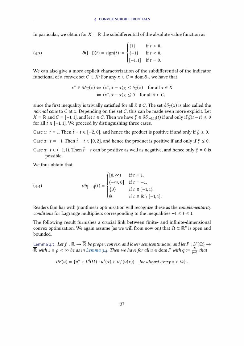
In particular, we obtain for X = R the subdierential of the absolute value function as

(4.3) ∂(| · |)(t) = sign(t) :=

1 if t > 0,

−1 if t < 0,

[−1, 1] if t = 0.

We can also give a more explicit characterization of the subdierential of the indicator

functional of a convex set C ⊂ X : For any x ∈ C = domδC , we have that

x∗ ∈ ∂δC(x) ⇔ 〈x∗, x − x〉X ≤ δC(x) for all x ∈ X

⇔ 〈x∗, x − x〉X ≤ 0 for all x ∈ C,

since the rst inequality is trivially satised for all x < C . The set ∂δC(x) is also called the

normal cone to C at x . Depending on the set C , this can be made even more explicit. Let

X = R andC = [−1, 1], and let t ∈ C . Then we have ξ ∈ ∂δ[−1,1](t) if and only if ξ (t − t) ≤ 0

for all t ∈ [−1, 1]. We proceed by distinguishing three cases.

Case 1: t = 1. Then t − t ∈ [−2, 0], and hence the product is positive if and only if ξ ≥ 0.

Case 2: t = −1. Then t − t ∈ [0, 2], and hence the product is positive if and only if ξ ≤ 0.

Case 3: t ∈ (−1, 1). Then t − t can be positive as well as negative, and hence only ξ = 0 is

possible.

We thus obtain that

(4.4) ∂δ[−1,1](t) =

[0,∞) if t = 1,

(−∞, 0] if t = −1,

0 if t ∈ (−1, 1),

∅ if t ∈ R \ [−1, 1].

Readers familiar with (non)linear optimization will recognize these as the complementarityconditions for Lagrange multipliers corresponding to the inequalities −1 ≤ t ≤ 1.

The following result furnishes a crucial link between nite- and innite-dimensional

convex optimization. We again assume (as we will from now on) that Ω ⊂ Rnis open and

bounded.

Lemma 4.7. Let f : R→ R be proper, convex, and lower semicontinuous, and let F : Lp(Ω) →R with 1 ≤ p < ∞ be as in Lemma 3.4. Then we have for all u ∈ dom F with q :=

pp−1

that

∂F (u) = u∗ ∈ Lq(Ω) : u∗(x) ∈ ∂ f (u(x)) for almost every x ∈ Ω .

37


Proof. Let u ∈ dom F , i.e., f u ∈ L1(Ω), and let u∗ ∈ Lp(Ω) be arbitrary. If u∗ ∈ Lq(Ω)satises u∗(x) ∈ ∂ f (u(x)) almost everywhere, we can insert u(x) into the denition and

integrate over all x ∈ Ω to obtain

F (u) − F (u) =

∫Ωf (u(x)) − f (u(x))dx ≥

∫Ωu∗(x)(u(x) − u(x))dx = 〈u∗, u − u〉Lp ,

i.e., u∗ ∈ ∂F (u).

Conversely, let u∗ ∈ ∂F (u). Then by denition it holds that∫Ωu∗(x)(u(x) − u(x))dx ≤

∫Ωf (u(x)) − f (u(x))dx for all u ∈ Lp(Ω).

Let now t ∈ R be arbitrary and let A ⊂ Ω be an arbitrary measurable set. Setting

u(x) :=

t if x ∈ A,

u(x) if x < A,

the above inequality implies due to u ∈ Lp(Ω) that∫Au∗(x)(t − u(x))dx ≤

∫Af (t) − f (u(x))dx .

Since A was arbitrary, it must hold that

u∗(x)(t − u(x)) ≤ f (t) − f (u(x)) for almost every x ∈ Ω.

Furthermore, since t ∈ R was arbitrary, we obtain that u∗(x) ∈ ∂u(x) for almost every

x ∈ Ω.

A similar proof shows that for F : RN → R with F (x) =∑N

i=1fi(xi) and fi : R→ R convex,

we have for any x ∈ dom F that

∂F (x) =ξ ∈ RN

: ξi ∈ ∂ fi(xi), 1 ≤ i ≤ N.

Together with the above examples, this yields componentwise expressions for the subdif-

ferential of the norm ‖ · ‖1 as well as of the indicator functional of the unit ball with respect

to the supremum norm in RN.

As for classical derivatives, one rarely obtains subdierentials from the fundamental deni-

tion but rather by applying calculus rules. It stands to reason that these are more dicult

to derive the weaker the derivative concept is (i.e., the more functionals are dierentiable

in that sense). For convex subdierentials, the following two rules still follow directly from

the denition.

38


Lemma 4.8. Let F : X → R be convex and x ∈ dom F . Then,

(i) ∂(λF )(x) = λ(∂F (x)) := λξ : ξ ∈ ∂F (x) for λ > 0;

(ii) ∂F (· + x0)(x) = ∂F (x + x0) for x0 ∈ X with x + x0 ∈ dom F .

The sum rule is already considerably more delicate.

Theorem 4.9 (sum rule). Let F ,G : X → R be convex and x ∈ dom F ∩ domG. Then,

∂F (x) + ∂G(x) ⊂ ∂(F +G)(x),

with equality if there exists an x0 ∈ (dom F )o ∩ domG.

Proof. The inclusion follows directly from adding the denitions of the two subdierentials.

Let therefore x ∈ dom F ∩ domG and ξ ∈ ∂(F +G)(x), i.e., satisfying

(4.5) 〈ξ , x − x〉X ≤ (F (x) +G(x)) − (F (x) +G(x)) for all x ∈ X .

Our goal is now to use (as in the proof of Lemma 3.6) the characterization of convex

functionals via their epigraph together with the Hahn–Banach separation theorem to

construct a bounded linear functional ζ ∈ ∂G(x) ⊂ X ∗ with ξ − ζ ∈ ∂F (x), i.e.,

F (x) − F (x) − 〈ξ , x − x〉X ≥ 〈ζ ,x − x〉X for all x ∈ dom F ,

G(x) −G(x) ≤ 〈ζ ,x − x〉X for all x ∈ domG .

For that purpose, we dene the sets

C1 := (x , t − (F (x) − 〈ξ ,x〉X )) : F (x) − 〈ξ , x〉X ≤ t ,

C2 := (x ,G(x) − t) : G(x) ≤ t ,

i.e.,

C1 = epi(F − ξ ) − (0, F (x) − 〈ξ ,x〉X ), C2 = −(epiG − (0,G(x))).

Since these are merely translations and, for C2, reections of epigraphs of proper convex

functionals, these sets are nonempty and convex. Furthermore, since x0 is an interior point

of dom F = dom(F − ξ ), the point (x0,α) for α suciently large is an interior point of C1.

Hence, (C1)o

is nonempty. It remains to show that (C1)o

and C2 are disjoint. But this holds

since any (x ,α) ∈ (C1)o ∩C2 satises by denition that

F (x) − F (x) − 〈ξ , x − x〉X < α ≤ G(x) −G(x),

contradicting (4.5). Corollary 1.6 therefore yields a pair (x∗, s) ∈ (X ×R)∗ \ (0, 0) and a

λ ∈ R with

〈x∗, x〉X + s(t − (F (x) − 〈ξ ,x〉X )) ≤ λ, x ∈ dom F , t ≥ F (x) − 〈ξ , x〉X ,(4.6)

〈x∗, x〉X + s(G(x) − t) ≥ λ, x ∈ domG, t ≥ G(x).(4.7)

39


We now show that s < 0. If s = 0, we can insert x = x0 ∈ dom F ∩ domG to obtain the

contradiction

〈x∗,x0〉X < λ ≤ 〈x∗,x0〉X ,

which follows since (x0,α) for α large enough is an interior point of C1 and hence can be

strictly separated from C2 by Theorem 1.5. If s > 0, choosing t > F (x) − 〈ξ ,x〉X makes the

term in parentheses in (4.6) strictly positive, and taking t → ∞ with xed x leads to a

contradiction to the boundedness by λ.

Hence s < 0, and (4.6) with t = F (x) − 〈ξ , x〉X and (4.7) with t = G(x) imply that

F (x) − F (x) + 〈ξ , x − x〉X ≥ s−1(λ − 〈x∗, x〉X ), for all x ∈ dom F ,

G(x) −G(x) ≤ s−1(λ − 〈x∗, x〉X ), for all x ∈ domG .

Taking x = x ∈ dom F ∩ domG in both inequalities immediately yields that λ = 〈x∗,x〉X .

Hence, ζ = s−1x∗ is the desired functional with (ξ − ζ ) ∈ ∂F (x) and ζ ∈ ∂G(x), i.e.,

ξ ∈ ∂F (x) + ∂G(x).

The following example demonstrates that the inclusion is strict in general (although

naturally the sitation in innite-dimensional vector spaces is nowhere near as obvious).

Example 4.10. We take again X = R and F : X → R from Example 4.10, i.e.,

F (x) =

−√x if x ≥ 0,

∞ if x < 0,

as well as G(x) = δ(−∞,0](x). Both F and G are convex, and 0 ∈ dom F ∩ domG . In fact,

(F +G)(x) = δ0(x) and hence it is straightforward to verify that ∂(F +G)(0) = R.

On the other hand, we know from Example 4.10 and the argument leading to (4.4) that

∂F (0) = ∅, ∂G(0) = [0,∞),

and hence that

∂F (0) + ∂G(0) = [0,∞) ( R = ∂(F +G)(0).

(As F only admits a vertical tangent as x = 0, this example corresponds to the situation

where s = 0 in (4.6).)

Remark 4.11. There exist alternative conditions that guarantee that the sum rule holds with equality.

For example, if X is a Banach space and F and G are in addition lower semicontinuous, this holds

under the Attouch–Brézis condition that⋃λ≥0

λ (dom F − domG) =: Z is a closed subspace of X ,

see [Attouch & Brezis 1986]. (Note that this condition is not satised in Example 4.10 either, since

in this case Z = − domG = [0,∞) which is closed but not a subspace.)

40


By induction, we obtain from this sum rules for an arbitrary (nite) number of functionals

(where x0 has to be an interior point of all but one eective domain). A chain rule for linear

operators can be proved similarly.

Theorem 4.12 (chain rule). LetA ∈ L(X ,Y ), F : Y → R be convex, and x ∈ dom(F A). Then,

∂(F A)(x) ⊃ A∗∂F (Ax) := A∗y∗ : y∗ ∈ ∂F (Ax)

with equality if there exists an x0 ∈ X with Ax0 ∈ (dom F )o .

Proof. The inclusion is again a direct consequence of the denition: If η ∈ ∂F (Ax) ⊂ Y ∗,we in particular have for all y = Ax ∈ Y with x ∈ X that

F (Ax) − F (Ax) ≥ 〈η,Ax −Ax〉Y = 〈A∗η, x − x〉X ,

i.e., ξ := A∗η ∈ ∂(F A) ⊂ X ∗.

Let now x ∈ dom(F A) and ξ ∈ ∂(F A)(x), i.e.,

F (Ax) + 〈ξ , x − x〉X ≤ F (Ax) for all x ∈ X .

As in the proof of a sum rule, we could now construct an η ∈ ∂F (Ax) with ξ = A∗η by

separating epi F and

graphA = (x ,Ax) : x ∈ X ⊂ X × Y .

For the sake of variety (and because the “lifting” technique we will use can be applied in

other contexts as well), we will instead apply the sum rule to

H : X × Y → R, (x ,y) 7→ F (y) + δgraphA(x ,y).

Since A is linear, graphA and hence δgraphA are convex. Furthermore, Ax ∈ dom F by

assumption and thus (x ,Ax) ∈ domH .

We begin by showing that ξ ∈ ∂(F A)(x) if and only if (ξ , 0) ∈ ∂H (x ,Ax). First, let

(ξ , 0) ∈ ∂H (x ,Ax). Then we have for all x ∈ X , y ∈ Y that

〈ξ , x − x〉X + 〈0, y −Ax〉Y ≤ F (y) − F (Ax) + δgraphA(x , y) − δgraphA(x ,Ax).

In particular, this holds for all y ∈ ran(A) = Ax : x ∈ X . By δgraphA(x ,Ax) = 0 we thus

obtain that

〈ξ , x − x〉X ≤ F (Ax) − F (Ax) for all x ∈ X ,

i.e., ξ ∈ ∂(F A)(x). Conversely, let ξ ∈ ∂(F A)(x). Since δgraphA(x ,Ax) = 0 and

δgraphA(x , y) ≥ 0, it then follows for all x ∈ X and y ∈ Y that

〈ξ , x − x〉X + 〈0, y −Ax〉Y = 〈ξ , x − x〉X

≤ F (Ax) − F (Ax) + δgraphA(x , y) − δgraphA(x ,Ax)

= F (y) − F (Ax) + δgraphA(x , y) − δgraphA(x ,Ax),

41


where we have used that last equality holds trivially as ∞ = ∞ for y , Ax . Hence,

(ξ , 0) ∈ ∂H (x ,Ax).

We now consider F : X × Y → R, (x ,y) 7→ F (y), and (x0,Ax0) ∈ graphA = domδgraphA.

Since Ax0 ∈ (dom F )o ⊂ Y by assumption, (x0,Ax0) ∈ (dom F )o as well. We can thus apply

Theorem 4.9 to obtain

(ξ , 0) ∈ ∂H (x ,Ax) = ∂F (Ax) + ∂δgraphA(x ,Ax),

i.e., (ξ , 0) = (x∗,y∗) + (w∗, z∗) for some (x∗,y∗) ∈ ∂F (Ax) and (w∗, z∗) ∈ ∂δgraphA(x ,Ax).

Now we have (x∗,y∗) ∈ ∂F (Ax) if and only if

〈x∗, x − x〉X + 〈y∗, y −Ax〉Y ≤ F (y) − F (Ax) for all x ∈ X , y ∈ Y .

Fixing x = x and y = Ax implies that y∗ ∈ ∂F (Ax) and x∗ = 0, respectively. Furthermore,

(w∗, z∗) ∈ ∂δgraphA(x ,Ax) if and only if

〈w∗, x − x〉X + 〈z∗, y −Ax〉Y ≤ 0 for all (x , y) ∈ graphA,

i.e., for all x ∈ X and y = Ax . Therefore,

〈w∗ +A∗z∗, x − x〉X ≤ 0 for all x ∈ X

and hence w∗ = −A∗z∗. Together we obtain

(ξ , 0) = (0,y∗) + (−A∗z∗, z∗),

which implies y∗ = −z∗ and thus ξ = −A∗z∗ = A∗y∗ with y∗ ∈ ∂F (Ax) as claimed.

The condition for equality in particular holds if A is surjective and dom F has non-empty

interior. Again, the inequality can be strict.

Example 4.13. Here we take X = Y = R and again F : X → R from Examples 4.3

and 4.10 as well as

A : R→ R, Ax = 0.

Clearly, (F A)(x) = 0 for all x ∈ R and hence ∂(F A)(x) = 0 by Theorem 4.5. On

the other hand, ∂F (0) = by Example 4.3 and hence

A∗∂F (Ax) = A∗∂F (0) =( 0.

(Note the problem: A is far from surjective, and ranA = 0 ∩ (dom F )o = ∅.)

The Fermat principle together with the sum rule yields the following characterization of

minimizers of convex functionals under convex constraints.

42


Corollary 4.14. Let U ⊂ X be nonempty, convex, and closed, and let F : X → R be proper,convex, and lower semicontinuous. If there exists an x0 ∈ U

o ∩ dom F , then x ∈ U solves

min

x∈UF (x)

if and only if there exists a ξ ∈ X ∗ with

(4.8)

− ξ ∈ ∂F (x),

〈ξ , x − x〉 ≤ 0 for all x ∈ U .

Proof. Since F and U are convex, we can apply Theorem 4.4 to J := F + δU . Furthermore,

since x0 ∈ Uo = (domδU )

o, we can also apply Theorem 4.9. Hence F has a minimum in x if

and only if

0 ∈ ∂J (x) = ∂F (x) + ∂δU (x).

Together with the characterization of subdierentials of indicator functionals as normal

cones, this yields (4.8).

If F : X → R is Gâteaux dierentiable (and hence nite-valued), (4.8) coincide with the

classical Karush–Kuhn–Tucker conditions; the existence of an interior point x0 ∈ U ois

exactly the Slater condition needed to show existence of the Lagrange multiplier ξ .

43

5 FENCHEL DUALITY

A particularly useful calculus rule connects the convex subdierential with the so-called

Fenchel–Legendre transform. Let X be a normed vector space and F : X → R be proper

but not necessarily convex. We then dene the Fenchel conjugate of F as

F ∗ : X ∗ → R, F ∗(x∗) = sup

x∈X〈x∗,x〉X − F (x).

(Since dom F , ∅ is excluded, we have that F ∗(x∗) > −∞ for all x∗ ∈ X ∗, and hence the

denition is meaningful.) Intuitively, F ∗(x∗) is the (negative of the) ane part of the tangent

to F (in the point x in which the supremum is attained) with slope x∗. Lemma 3.5 (v) and

Lemma 2.2 (v) immediately imply that F ∗ is always convex and lower semicontinuous (as

long as F is indeed proper). If F is bounded from below by an ane functional (which is

always the case if F is proper, convex, and lower semicontinuous by Lemma 3.6), then F ∗

is proper as well. Finally, the denition directly yields the Fenchel–Young inequality

(5.1) 〈x∗,x〉X ≤ F (x) + F ∗(x∗) for all x ∈ X ,x∗ ∈ X ∗.

If X is not reexive, we can similarly dene the Fenchel preconjugate

F∗ : X → R, F ∗(x) = sup

x∗∈X ∗〈x∗,x〉X − F (x

∗).

The point of this convention is that even in non-reexive spaces, the biconjugate

F ∗∗ : X → R, F ∗∗(x) = (F ∗)∗(x)

is again dened on X (rather than X ∗∗ ⊃ X ). For reexive spaces, of course, we have

F ∗∗ = (F ∗)∗. Intuitively, F ∗∗ is the convex hull of F , which by Lemma 3.6 coincides with Fitself if F is convex.

Theorem 5.1 (Fenchel–Moreau–Rockafellar). Let F : X → R be proper. Then,

(i) F ∗∗ ≤ F ;

(ii) F ∗∗ = F Γ ;

(iii) F ∗∗ = F if and only if F is convex and lower semicontinuous.

44

5 fenchel duality

Proof. For (i), we take the supremum over all x∗ ∈ X ∗ in the Fenchel–Young inequality (5.1)

and obtain that

F (x) ≥ sup

x∗∈X ∗〈x∗,x〉X − F

∗(x∗) = F ∗∗(x).

For (ii), we rst note that F ∗∗ is convex and lower semicontinuous by denition as a Fenchel

conjugate as well as proper by (i). Hence, Lemma 3.6 yields that

F ∗∗(x) = (F ∗∗)Γ(x) = sup a(x) : a : X → R ane with a ≤ F ∗∗ .

We now show that we can replace F ∗∗ with F on the right-hand side. For this, let a(x) =〈x∗,x〉X − α with arbitrary x∗ ∈ X ∗ and α ∈ R. If a ≤ F ∗∗, then (i) implies that a ≤ F .

Conversely, if a ≤ F , we have that 〈x∗,x〉X − F (x) ≤ α for all x ∈ X , and taking the

supremum over all x ∈ X yields that α ≥ F ∗(x∗). By denition of F ∗∗, we thus obtain that

a(x) = 〈x∗,x〉X − α ≤ 〈x∗,x〉X − F

∗(x∗) ≤ F ∗∗(x) for all x ∈ X ,

i.e., a ≤ F ∗∗.

Statement (iii) now directly follows from (ii) and Lemma 3.6.

We again consider some relevant examples.

Example 5.2.

(i) LetX be a Hilbert space and F (x) = 1

2‖x ‖2X . Using the Fréchet–Riesz Theorem 1.12,

we identifyX with its dualX ∗ and can express the duality pairing using the inner

product. Since F is Fréchet dierentiable with gradient ∇F (x) = x , the solution

x ∈ X to

sup

x∈X(x∗,x)X −

1

2(x ,x)X

for given x∗ ∈ X has to satisfy the Fermat principle, i.e., x = x∗. Inserting this

into the denition and simplifying yields the Fenchel conjugate

F ∗ : X → R, F ∗(x∗) = 1

2‖x∗‖2X .

(ii) Let BX be the unit ball in the normed vector space X and take F = δBX . Then we

have for any x∗ ∈ X ∗ that

(δBX )∗(x∗) = sup

x∈X〈x∗,x〉X − δBX (x) = sup

‖x ‖X ≤1

〈x∗,x〉X = ‖x∗‖X ∗ .

Similarly, one shows using the denition of the Fenchel conjugate in dual spaces

and Corollary 1.7 that (δBX ∗ )∗(x) = ‖x ‖X .

(iii) Let X be a normed vector space and take F (x) = ‖x ‖X . We now distinguish two

cases for a given x∗ ∈ X ∗.

45

5 fenchel duality

Case 1: ‖x∗‖X ∗ ≤ 1. Then it follows from (1.1) that 〈x∗,x〉X − ‖x ‖X ≤ 0 for all

x ∈ X . Furthermore, 〈x∗, 0〉 = 0 = ‖0‖X , which implies that

F ∗(x∗) = sup

x∈X〈x∗,x〉X − ‖x ‖X = 0.

Case 2: ‖x∗‖X ∗ > 1. Then by denition of the dual norm, there exists an x0 ∈ Xwith 〈x∗,x0〉X > ‖x0‖X . Hence, taking t →∞ in

0 < t(〈x∗,x0〉X − ‖x0‖X ) = 〈x∗, tx0〉X − ‖tx0‖X ≤ F ∗(x∗)

yields F ∗(x∗) = ∞.

Together we obtain that F ∗ = δBX ∗ . As above, a similar argument shows that

(‖ · ‖X ∗)∗ = δBX .

Fenchel conjugates satisfy a number of useful calculus rules, which follow directly from

the properties of the supremum.

Lemma 5.3. Let F : X → R be proper. Then,

(i) (αF )∗ = αF ∗ (α−1Id) for any α > 0;

(ii) (F (· + x0) + 〈x∗0, ·〉X )

∗ = F ∗(· − x∗0) − 〈· − x∗

0,x0〉X for all x0 ∈ X , x∗

0∈ X ∗;

(iii) (F A)∗ = F ∗ A−∗ for continuously invertible A ∈ L(Y ,X ) and A−∗ := (A−1)∗.

Proof. Ad (i): For any α > 0, we have that

(αF )∗(x∗) = sup

x∈X

(α 〈α−1x∗,x〉X − αF (x)

)= α sup

x∈X

(〈α−1x∗,x〉X − F (x)

)= αF ∗(α−1x∗).

Ad (ii): Since x + x0 : x ∈ X = X , we have that

(F (· + x0) + 〈x∗0, ·〉X )

∗(x∗) = sup

x∈X〈x∗,x〉X − F (x

∗ + x0) − 〈x∗0,x0〉X

= sup

x∈X

(〈x∗ − x∗

0,x + x0〉X − F (x

∗ + x0))− 〈x∗ − x∗

0,x0〉X

= sup

x=x+x0,x∈X

(〈x∗ − x∗

0, x〉X − F (x)

)− 〈x∗ − x∗

0,x0〉X

= F ∗(x∗ − x∗0) − 〈x∗ − x∗

0,x0〉X .

Ad (iii): Since X = ranA, we have that

(F A)∗(y∗) = sup

y∈Y〈y∗,A−1Ay〉Y − F (Ay)

= sup

x=Ay ,y∈Y〈A−∗y∗,x〉X − F (x) = F ∗(A−∗y∗).

46

5 fenchel duality

As in Lemma 4.7,1

one can show that Fenchel conjugates of integral functionals can be

computed pointwise; see, e.g., [Rockafellar 1976, Theorem 3C].

Lemma 5.4. Let f : R → R be measurable, proper and lower semicontinuous, and letF : Lp(Ω) → R with 1 ≤ p < ∞ be dened as in Lemma 3.4. Then we have for q = p

p−1that

F ∗ : Lq(Ω) → R, F ∗(u∗) =

∫Ωf ∗(u∗(x))dx .

There are some obvious similarities between the denitions of the Fenchel conjugate and

of the subdierential, which yield the following very useful property.

Lemma 5.5. Let F : X → R be proper, convex, and lower semicontinuous. Then the followingstatements are equivalent for any x ∈ X and x∗ ∈ X ∗:

(i) 〈x∗,x〉X = F (x) + F ∗(x∗);

(ii) x∗ ∈ ∂F (x);

(iii) x ∈ ∂F ∗(x∗).

Proof. If (i) holds, the denition of F ∗ as a supremum immediately implies that

(5.2) 〈x∗,x〉X − F (x) = F ∗(x∗) ≥ 〈x∗, x〉X − F (x) for all x ∈ X ,

which again by denition is equivalent to x∗ ∈ ∂F (x). Conversely, taking the supremum

over all x ∈ X in (5.2) yields

〈x∗,x〉X ≥ F (x) + F ∗(x∗),

which together with the Fenchel–Young inequality (5.1) leads to (i).

Similarly, (i) in combination with Theorem 5.1 yields that for all x∗ ∈ X ∗,

〈x∗,x〉X − F∗(x∗) = F (x) = F ∗∗(x) ≥ 〈x∗,x〉 − F ∗(x∗),

yielding as above the equivalence of (i) and (iii).

Remark 5.6. If X is not reexive, x ∈ ∂F ∗(x∗) ⊂ X ∗∗ in (iii) has to be understood via the canonical

injection, i.e., as

〈J (x), x∗ − x∗〉X ∗ = 〈x∗ − x∗,x〉X ≤ F ∗(x∗) − F ∗(x∗) for all x∗ ∈ X .

Using (iii) to conclude equality in (i) or, equivalently, the subdierential inclusion (ii) therefore

requires the additional condition that x ∈ X ⊂ X ∗∗. Conversely, if (i) or (ii) hold, (iii) also guarantees

that the subderivative x ∈ ∂F ∗(x∗) ∩ X , which is a stronger fact. (Similar statements apply to

F : X ∗ → R and F∗ : X → R.)

1modulo some technical diculties since measurability of f u does not immediately imply that of f ∗ u∗

47

5 fenchel duality

Lemma 5.5 plays the role of a “convex inverse function theorem”, and can be used to,

e.g., replace the subdierential of a (complicated) norm with that of a (simpler) conjugate

indicator functional (or vice versa). For example, given a problem of the form

(5.3) inf

x∈XF (x) +G(Ax)

for F : X → R andG : Y → R proper, convex, and lower semicontinuous, and A ∈ L(X ,Y ),we can use Theorem 5.1 to replace G with the denition of G∗∗ and obtain

inf

x∈Xsup

Y ∗∈Y ∗F (x) + 〈y∗,Ax〉Y −G

∗(y∗).

If(!) we were now able to exchange inf and sup, we could write (with inf F = − sup(−F ))

inf

x∈Xsup

y∗∈y∗F (x) + 〈y∗,Ax〉Y −G

∗(y∗) = sup

y∗∈Y ∗inf

x∈XF (x) + 〈y∗,Ax〉Y −G

∗(y∗)

= sup

y∗∈Y ∗−

(sup

x∈X−F (x) + 〈−A∗y∗,x〉X

)−G∗(y∗).

By denition of F ∗, we thus obtain the dual problem

(5.4) sup

y∗∈Y ∗−F ∗(−A∗y∗) −G∗(y∗).

As a side eect, we have shifted the operator A from G to F ∗ without having to invert it.

The following theorem in an elegant way uses the Fermat principle, the sum and chain rules,

and the Fenchel–Young equation to derive sucient conditions for the exchangeability.

Theorem 5.7 (Fenchel–Rockafellar). Let X and Y be normed vector spaces, F : X → R

and G : Y → R be proper, convex, and lower semicontinuous, and A ∈ L(X ,Y ). Assumefurthermore that

(i) the primal problem (5.3) admits a solution x ∈ X ;

(ii) there exists an x0 ∈ dom F ∩ dom(G A) with Ax0 ∈ (domG)o .

Then, the dual problem (5.4) admits a solution y∗ ∈ Y ∗ and

(5.5) min

x∈XF (x) +G(Ax) = max

y∗∈Y ∗−F ∗(−A∗y∗) −G∗(y∗).

Furthermore, x and y∗ are solutions to (5.3) and (5.4), respectively, if and only if

(5.6)

−A∗y∗ ∈ ∂F (x),

y∗ ∈ ∂G(Ax).

48

5 fenchel duality

Proof. Theorem 4.4 states that x ∈ X is a solution to (5.3) if and only if 0 ∈ ∂(F +G A)(x).By assumption (ii), Theorems 4.9 and 4.12 are applicable, and we thus obtain that

0 ∈ ∂(F +G A)(x) = ∂F (x) +A∗∂G(Ax),

which implies that there exists a y∗ ∈ ∂G(Ax) with −A∗y∗ ∈ ∂F (x), i.e., satisfying (5.6).

The relations (5.6) together with Lemma 5.5 further imply equality in the Fenchel–Young

inequalities for F and G, i.e.,

(5.7)

〈−A∗y∗, x〉X = F (x) + F ∗(−A∗y∗),

〈y∗,Ax〉Y = G(Ax) +G∗(y∗).

Adding both equations now yields

(5.8) F (x) +G(Ax) = −F ∗(−A∗y∗) −G∗(y∗).

It remains to show that y∗ is a solution to (5.4). For this purpose, we introduce

L : X × Y ∗ → R, L(x ,y∗) = F (x) + 〈y∗,Ax〉Y −G∗(y∗).

For all x ∈ X and y∗ ∈ Y ∗, we always have that

sup

y∗∈Y ∗L(x ,y∗) ≥ L(x , y∗) ≥ inf

x∈XL(x , y∗),

and hence (taking the inmum over all x in the rst and the supremum over all y∗ in the

second inequality) that

inf

x∈Xsup

y∗∈Y ∗L(x ,y∗) ≥ sup

y∗∈Y ∗inf

x∈XL(x ,y∗).

We thus obtain that

F (x) +G(Ax) = inf

x∈Xsup

Y ∗∈Y ∗F (x) + 〈y∗,Ax〉Y −G

∗(y∗)

≥ sup

Y ∗∈Y ∗inf

x∈XF (x) + 〈y∗,Ax〉Y −G

∗(y∗)

= sup

y∗∈Y ∗−F ∗(−A∗y∗) −G∗(y∗).

Combining this with (5.8) yields that

− F ∗(−A∗y∗) −G(y∗) = F (x) +G(Ax) ≥ sup

y∗∈Y ∗−F ∗(−A∗y∗) −G∗(y∗),

i.e., y∗ is a solution to (5.4), and hence (5.5) follows from (5.8).

Finally, if x ∈ X and y∗ ∈ Y ∗ are solutions to (5.3) and (5.4), respectively, then (5.5) implies

(5.8). Together with the productive zero, this implies that

0 = [F (x) + F ∗(−A∗y∗) − 〈−A∗y∗, x〉X ] + [G(Ax) +G∗(y∗) − 〈y∗,Ax〉Y ] .

Since both brackets have to be nonnegative due to the Fenchel–Young inequality, they each

have to be zero. We therefore deduce that (5.7) holds, and hence Lemma 5.5 implies (5.6).

49

5 fenchel duality

The relations (5.6) are referred to as Fenchel extremality conditions; we can use Lemma 5.5

to generate further, equivalent, optimality conditions by inverting one or the other sub-

dierential inclusion. We will later exploit this to derive implementable algorithms for

solving optimization problems of the form (5.3).

50

6 MONOTONE OPERATORS AND PROXIMAL POINTS

Any minimizer x ∈ X of the convex functional F : X → R satises by Theorem 4.4

the Fermat principle 0 ∈ ∂F (x). To obtain from this useful information about (and, later,

implementable algorithms for the computation of) x , we thus have to study the mapping

x 7→ ∂F (x). To avoid technical diculties – and since we will use the following results

mainly for numerical algorithms, i.e., for X = RN– we restrict the discussion in this and

the next chapter to Hilbert spaces (but see Remark 6.17 below). This allows identifying X ∗

with X ; in particular, we will from now on identify the set ∂F (x) ⊂ X ∗ of subderivatives

with the corresponding set in X of subgradients (i.e., their Riesz representations).

6.1 monotone operators

For two normed vector spaces X and Y we consider a set-valued mapping A : X → P(Y ),also denoted by A : X ⇒ Y , and dene

• its domain of denition domA = x ∈ X : Ax , ∅;

• its range ranA =⋃

x∈X Ax ;

• its graph graphA = (x ,y) ∈ X × Y : y ∈ Ax;

• its inverse A−1: Y ⇒ X via A−1(y) = x ∈ X : y ∈ Ax for all y ∈ Y .

(Note that A−1(y) = ∅ is allowed by the denition; hence for set-valued mappings, their

inverse and preimage – which always exists – coincide.)

For A,B : X ⇒ Y , C : Y ⇒ Z , and λ ∈ R we further dene

• λA : X ⇒ Y via (λA)(x) = λy : y ∈ Ax;

• A + B : X ⇒ Y via (A + B)(x) = y + z : y ∈ Ax , z ∈ Bx;

• C A : X ⇒ Z via (C A)(x) = z : there is y ∈ Ax with z ∈ Cy.

51

6 monotone operators and proximal points

A set-valued mapping A : X ⇒ X is called monotone if graphA , ∅ (to exclude trivial

cases) and

(6.1)

(x∗

1− x∗

2,x1 − x2

)X ≥ 0 for all (x1,x

∗1), (x2,x

∗2) ∈ graphA.

Obviously, the identity mapping Id : X ⇒ X , x 7→ x, is monotone. If F : X → R is

convex, then ∂F : X ⇒ X , x 7→ ∂F (x), is monotone: For any x1,x2 ∈ X with x∗1∈ ∂F (x1)

and x∗2∈ ∂F (x2), we have by denition that(

x∗1, x − x1

)X ≤ F (x) − F (x1) for all x ∈ X ,(

x∗2, x − x2

)X ≤ F (x) − F (x2) for all x ∈ X .

Adding the rst inequality for x = x2 and the second for x = x1 and rearranging the result

yields (6.1). Furthermore, if A,B : X ⇒ X are monotone and λ ≥ 0, then λA and A + B are

monotone as well.

In fact, we will need the following, stronger, property, which guarantees thatA is continuous

in an appropriate sense: A monotone operator A : X ⇒ X is called maximally monotone, if

for any x ∈ X and x∗ ∈ X the condition

(6.2) (x∗ − x∗,x − x)X ≥ 0 for all (x , x∗) ∈ graphA

implies that x∗ ∈ Ax . (In other words, (6.2) holds if and only if (x ,x∗) ∈ graphA.) For xed

x ∈ X and x∗ ∈ X , the condition claims that if A is monotone, so is the extension

A : X ⇒ X , x 7→

Ax ∪ x∗ if x = x ,

Ax if x , x .

For A to be maximally monotone means that this is not a true extension, i.e., A = A. For

example, the operator

A : R⇒ R, t 7→

1 if t > 0,

0 if t = 0,

−1 if t < 0,

is monotone but not maximally monotone, since A is a proper subset of the monotone

operator dened by At = sign(t) = ∂(| · |)(t).

Several useful properties follow directly from the denition.

Lemma 6.1. If A : X ⇒ X is maximally monotone and λ > 0, so is λA for all λ > 0.

Proof. Let x ,x∗ ∈ X and assume that

0 ≤ (x∗ − x∗,x − x)X = λ(λ−1x∗ − λ−1x∗,x − x

)X for all (x , x∗) ∈ graph λA.

Since x∗ ∈ λAx if and only if λ−1x∗ ∈ Ax and A is maximally monotone, this implies that

λ−1x∗ ∈ Ax , i.e., x∗ ∈ (λA)x . Hence, λA is maximally monotone.

52


We now come to the promised continuity property. We call a set-valued mappingA : X ⇒ Xouter semicontinuous ifxn → x andAxn 3 x

∗n → x∗ imply thatx∗ ∈ Ax . If either convergence

is not strong, we explicitly state the topology as in the following

Lemma 6.2. Let A : X ⇒ X be maximally monotone. Then A is weak-to-strong outersemicontinuous.

Proof. For arbitrary x ∈ X and x∗ ∈ Ax , the monotonicity of A implies that

0 ≤(x∗n − x

∗,xn − x)X → (x

∗ − x∗,x − x)X

since the duality pairing and hence the inner product of weakly and strongly converging

sequences is convergent. Since A is maximally monotone, we obtain that x∗ ∈ Ax .

Of central importance to the theory of monotone operators is Minty’s theorem, which states

that a monotone operator A is maximally monotone if and only if Id +A is surjective. As a

preparation, we rst prove an important partial result.

Lemma 6.3. Let F : X → R be proper, convex and lower semicontinuous. Then Id + ∂F issurjective.

Proof. We consider for given z ∈ X the functional

J : X → R, x 7→1

2

‖x − z‖2X + F (x),

which is proper, (strictly) convex and lower semicontinuous by the assumptions on F .

Furthermore, J is coercive by Lemma 3.8. Theorem 3.7 thus yields a (unique) x ∈ X with

J (x) = minx∈X J (x), which by Theorems 4.4, 4.5 and 4.9 satises that

0 ∈ ∂J (x) = x − z + ∂F (x),

i.e., z ∈ x + ∂F (x) = (Id + ∂F )(x).

We now turn to the general case.

Theorem 6.4 (Minty). Let A : X ⇒ X be monotone. Then, A is maximally monotone if andonly if Id +A is surjective.

Proof. First, assume that Id +A is surjective, and consider x ∈ X and x∗ ∈ X with

(6.3) (x∗ − x∗,x − x)X ≥ 0 for all (x , x∗) ∈ graphA.

The assumption now implies that for x + x∗ ∈ X , there exist a z ∈ X and a z∗ ∈ Az with

(6.4) x + x∗ = z + z∗ ∈ (Id +A)z.

53


Inserting (x , x∗) = (z, z∗) into (6.3) then yields that

0 ≤ (x∗ − z∗,x − z)X = (z − x ,x − z)X = −‖x − z‖2

X ≤ 0,

i.e., x = z. From (6.4) we further obtain x∗ = z∗ ∈ Az = Ax , and hence A is maximally

monotone.

The proof of the converse implication is signicantly more involved. The special case

A = ∂F for a convex functional F was already shown in Lemma 6.3; for the general case,

we proceed similarly by constructing a functional FA that plays the same role for A as Fdoes for ∂F . Specically, we dene for a maximally monotone operator A : X ⇒ X the

Fitzpatrick functional

(6.5) FA : X × X → [−∞,∞], (x ,y) 7→ sup

(z,w)∈graphA

((z,y)X + (x ,w)X − (z,w)X

),

which can be written equivalently as

(6.6) FA(x ,y) = (x ,y)X − inf

(z,w)∈graphA(x − z,y −w)X .

Each characterization implies useful properties.

(i) By maximal monotonicity of A, we have by denition that (x − z,y −w)X ≥ 0 for all

(z,w) ∈ graphA if and only if (x ,y) ∈ graphA; in particular, (x − z,y −w)X < 0 for

all (x ,y) < graphA. Hence, (6.6) implies that FA(x ,y) ≥ (x ,y)X , with equality if and

only if (x ,y) ∈ graphA (since in this case the inmum is attained in (z,w) = (x ,y)).In particular, FA is proper.

(ii) On the other hand, the denition (6.5) yields that

FA = (GA)∗

for GA(w, z) = (w, z)X + δgraphA−1(w, z)

(since (z,w) ∈ graphA if and only if (w, z) ∈ graphA−1). As part of the monotonicity

of A, we have required that graphA , ∅; hence FA is the Fenchel conjugate of a

proper functional and therefore convex and lower semicontinuous.

As a rst step, we now show the result for the special case z = 0, i.e., that 0 ∈ ran(Id +A).We now set Z := X × X as well as ξ := (x ,y) and consider the functional

JA : Z → R, ξ 7→ FA(ξ ) +1

2

‖ξ ‖2Z .

We rst note that property (i) implies for all ξ ∈ Z that

(6.7) JA(ξ ) = FA(ξ ) +1

2

‖ξ ‖2Z = FA(x ,y) +1

2

‖x ‖2X +1

2

‖y ‖2X

≥ (x ,y)X +1

2

‖x ‖2X +1

2

‖y ‖2X

≥ 0.

54


Furthermore, JA is proper, (strictly) convex, lower semicontinuous, and (by Lemma 3.8)

coercive. Theorem 3.7 thus yields a (unique)¯ξ := (x , y) ∈ Z with JA( ¯ξ ) = minξ∈Z JA(ξ ),

which by Theorems 4.4, 4.5 and 4.9 satises that

0 ∈ ∂JA( ¯ξ ) = ¯ξ + ∂FA( ¯ξ ),

i.e., − ¯ξ ∈ ∂FA( ¯ξ ). By denition of the subdierential, we thus have for all ξ ∈ Z that

FA(ξ ) ≥ FA( ¯ξ ) +(− ¯ξ , ξ − ¯ξ

)Z = JA(

¯ξ ) +1

2

‖− ¯ξ ‖2Z +(− ¯ξ , ξ

)Z

≥1

2

‖− ¯ξ ‖2Z +(− ¯ξ , ξ

)Z ,

where the last step follows from (6.7). For the sake of presentation, we will replace¯ξ 7→ − ¯ξ

from now on; property (i) then implies for all (x ,y) ∈ graphA that

(6.8) (x ,y)X = FA(x ,y) ≥1

2

‖x ‖2X + (x ,x)X +1

2

‖y ‖2X + (y,y)X

≥ − (x , y)X + (x ,x)X + (y,y)X ,

and hence (y − x ,x − y)X ≥ 0. The maximal monotonicity of A thus yields that x ∈ Ay ,

i.e., (y, x) ∈ graphA. Inserting this into the rst inequality of (6.8) then implies that

(y, x)X ≥1

2

‖x ‖2X + (x , y)X +1

2

‖y ‖2X + (y, x)X =1

2

‖x + y ‖2X + (y, x)X ≥ (y, x)X

and hence ‖x + y ‖X = 0, i.e., 0 = y + x ∈ (Id +A)(y).

Finally, let z ∈ X be arbitrary and set B : X ⇒ X , x 7→ −z +Ax . Using the denition, it

is straightforward to verify that B is maximally monotone as well. As we have just shown,

there now exists a y ∈ X with 0 ∈ (Id + B)(y) = y + −z + Ay , i.e., z ∈ (Id + A)(y).Hence Id +A is surjective.

Together with Lemma 6.3, this yields the maximal monotonicity of convex subdieren-

tials.

Corollary 6.5. Let F : X → R be proper, convex, and lower semicontinuous. Then ∂F : X ⇒ Xis maximally monotone.

6.2 resolvents and proximal points

We know from Lemma 6.3 that Id + ∂F is surjective for any proper, convex, and lower

semicontinuous functional F ; the proof even shows that each preimage is unique. Hence

(Id+ ∂F )−1is single-valued even if ∂F is not. We can thus hope to use this object instead of

a subdierential – or, more generally, a maximally monotone operator – for algorithms.

55


We thus dene for a maximally monotone operator A : X ⇒ X the resolvent

RA : X ⇒ X , RA(x) = (Id +A)−1x ,

as well as for a proper, convex, and lower semicontinuous functional F : X → R the

proximal point mapping

(6.9) proxF : X → X , proxF (x) = arg min

z∈X

1

2

‖z − x ‖2X + F (z).

Since w ∈ R∂F (x) are the necessary and sucient conditions for the proximal point w to

be a minimizer of the strictly convex functional in (6.9), we have that

(6.10) proxF = (Id + ∂F )−1 = R∂F .

It remains to show that the resolvent of arbitrary maximally monotone operators is single-

valued on X as well and we can thus write RA : X → X .

Lemma 6.6. Let A : X ⇒ X be maximally monotone. Then RA : X → X .

Proof. Since A is maximally monotone, Id+A is surjective, which implies that domRA = X .

Let now x , z ∈ X with x∗ ∈ RA(x) and z∗ ∈ RA(z), i.e., x ∈ x∗ +Ax∗ and z ∈ z∗ +Az∗.For x − x∗ ∈ Ax∗ and z − z∗ ∈ Az∗, the monotonicity of A implies that

(6.11) ‖x∗ − z∗‖2X ≤ (x − z,x∗ − z∗)X .

Hence x = z implies x∗ = z∗, i.e., RA is single-valued.

The inequality (6.11) together with the Cauchy–Schwarz inequality shows that resolvents

are Lipschitz continuous with constant L = 1; such mappings are called nonexpansive. Since

(6.11) is in fact a stronger property, a mapping T : X → X is called rmly nonexpansive if it

satises this inequality, i.e., if

‖Tx −Tz‖2X ≤ (Tx −Tz,x − z)X for all x , z ∈ X .

Firm nonexpansivity implies another useful inequality.

Lemma 6.7. Let A : X ⇒ X be maximally monotone. Then RA : X → X is rmly nonexpan-sive and satises that

‖RAx − RAz‖2

X + ‖(Id − RA)x − (Id − RA)z‖2

X ≤ ‖x − z‖2

X for all x , z ∈ X .

Proof. Firm nonexpansivity of RA was already shown in (6.11), which further implies that

‖(Id − RA)x − (Id − RA)z‖2

X = ‖x − z‖2

X − 2 (x − z,RAx − RAz)X + ‖RAx − RAz‖2

X

≤ ‖x − z‖2X − ‖RAx − RAz‖2

X .

56


Corollary 6.8. Let F : X → R be proper, convex, and lower semicontinuous. Then proxF :

X → X is Lipschitz continuous with constant L = 1.

The following useful result allows characterizing minimizers of convex functionals as

proximal points.

Lemma 6.9. Let F : X → R be proper, convex, and lower semicontinuous, and x ,x∗ ∈ X . Thenfor any γ > 0,

x∗ ∈ ∂F (x) ⇔ x = proxγF (x + γx∗).

Proof. Multiplying both sides of the subdierential inclusion by γ > 0 and adding x yields

that

x∗ ∈ ∂F (x) ⇔ x + γx∗ ∈ (Id + γ ∂F )(x)

⇔ x ∈ (Id + γ ∂F )−1(x + γx∗)

⇔ x = proxγF (x + γx∗),

where in the last step we have used that γ ∂F = ∂(γF ) by Lemma 4.8 (ii) and hence that

proxγF = Rγ ∂F .

Corollary 6.10. Let F : X → R be proper, convex and lower semicontinuous, and γ > 0 bearbitrary. Then x ∈ dom F is a minimizer of F if and only if

x = proxγF (x).

Proof. Simply apply Lemma 6.9 to the Fermat principle 0 ∈ ∂F (x).

This simple result should not be underestimated: It allows replacing (explicit) set inclusions

by (implicit) Lipschitz continuous equations in optimality conditions, thus opening the

door to xed point iterations or Newton methods.

We can also derive a generalization of the orthogonal decomposition of vector spaces.

Theorem 6.11 (Moreau decomposition). Let F : X → R be proper, convex, and lower semi-continuous. Then we have for all x ∈ X that

x = proxF (x) + proxF ∗(x).

Proof. Setting w = proxF (x), Lemmas 5.5 and 6.9 imply that

w = proxF (x) = proxF (w + (x −w)) ⇔ x −w ∈ ∂F (w)

⇔ w ∈ ∂F ∗(x −w)

⇔ x −w = proxF ∗((x −w) +w) = proxF ∗(x).

57


The following calculus rules will prove useful.

Lemma 6.12. Let F : X → R be proper, convex, and lower semicontinuous. Then,

(i) for λ , 0 and z ∈ X we have with H (x) := F (λx + z) that

proxH (x) = λ−1(proxλ2F (λx + z) − z);

(ii) for γ > 0 we have thatproxγF ∗(x) = x − γ proxγ−1F (γ

−1x);

(iii) for proper, convex, lower semicontinuousG : Y → R andγ > 0 we have withH (x ,y) :=

F (x) +G(y) that

proxγH (x ,y) =

(proxγF (x)

proxγG(y)

).

Proof. Ad (i): By denition,

proxH (x) = arg min

w∈X

1

2

‖w − x ‖2X + F (λw + z) =: w .

Substituting v = λw + z and using that minw∈X G(w) = minv∈X G(v) for all G implies that

v = arg min

v∈X

1

2

‖λ−1(v − z) − x ‖2X + F (v)

= arg min

v∈X

1

2λ2‖v − (λx + z)‖2X + F (v)

= arg min

v∈X

1

2

‖v − (λx + z)‖2X + λ2F (v)

= proxλ2F (λx + z).

Hence, w := λ−1(v − z) is the desired minimizer.

Ad (ii): Theorem 6.11, Lemma 5.3 (i), and (i) for λ = γ−1and z = 0 together imply that

proxγF (x) = x − prox(γF )∗(x)

= x − proxγF ∗(γ−1Id)(x)

= x − γ proxγ (γ−2F ∗)(γ−1x).

Applying this to F ∗ and using that F ∗∗ = F now yields the claim.

Ad (iii): By denition of the norm on the product space X × Y , we have that

proxγH (x ,y) = arg min

(u,v)∈X×Y

1

2

‖(u,v) − (x ,y)‖2X×Y + γH (u,v)

= arg min

u∈X ,v∈Y

(1

2

‖u − x ‖2X + γF (u)

)+

(1

2

‖v − y ‖2Y + γG(v)

).

58


Since there are no mixed terms in u and v , the two terms in parentheses can be minimized

separately. Hence, proxγH (x ,y) = (u, v) for

u = arg min

u∈X

1

2

‖u − x ‖2X + γF (u) = proxγF (x),

v = arg min

v∈Y

1

2

‖v − y ‖2Y + γG(v) = proxγG(x).

Computing proximal points is dicult in general since evaluating proxF by its denition

entails minimizing F . In some cases, however, it is possible to give an explicit formula for

proxF .

Example 6.13. We rst consider scalar functions f : R→ R.

(i) f (t) = 1

2|t |2. Since f is dierentiable, we can set the derivative of

1

2(s − t)2 +

γ2s2

to zero and solve for s to obtain proxγ f (t) = (1 + γ )−1t .

(ii) f (t) = |t |. By (4.3) we have that ∂ f (t) = sign(t); hence s := proxγ f (t) = (Id +

γ sign)−1(t) if and only if t ∈ s+γ sign(s). Let t be given and assume this holds

for some s . We now proceed by case distinction.

Case 1: s > 0. This implies that t = s + γ , i.e., s = t − γ , and hence that t > γ .

Case 2: s < 0. This implies that t = s − γ , i.e., s = t + γ , and hence that t < −γ .

Case 3: s = 0. This implies that t ∈ γ [−1, 1] = [−γ ,γ ].

Since this yields a complete and disjoint case distinction for t , we can conclude

that

proxγ f (t) =

t − γ if t > γ ,

0 if t ∈ [−γ ,γ ],

t + γ if t < −γ .

This mapping is also known as the soft-shrinkage or soft-thresholding operator.

(iii) f (t) = δ[−1,1](t). By Example 5.2 (iii) we have that f ∗(t) = |t |, and hence Lemma 6.12 (ii)

59


yields that

proxγ f (t) = t − γ proxγ−1 f ∗(γ−1t)

=

t − γ (γ−1t − γ−1) if γ−1t > γ−1,

t − 0 if γ−1t ∈ [−γ−1,γ−1],

t − γ (γ−1t + γ−1) if γ−1t < −γ−1

=

1 if t > 1,

t if t ∈ [−1, 1],

−1 if t < −1.

For every γ > 0, the proximal point of t is thus its projection onto [−1, 1].

Example 6.14. We can generalize Example 6.13 toX = RN(endowed with the Euclidean

inner product) by applying Lemma 6.12 (iii) N times. We thus obtain componentwise

(i) for F (x) = 1

2‖x ‖2

2=

∑Ni=1

1

2x2

i that

[proxγF (x)]i =

(1

1 + γ

)xi , 1 ≤ i ≤ N ;

(ii) for F (x) = ‖x ‖1 =∑N

i=1|xi | that

[proxγF (x)]i = (|xi | − γ )+

sign(xi), 1 ≤ i ≤ N ;

(iii) for F (x) = δB∞(x) =∑N

i=1δ[−1,1](xi) that

[proxγF (x)]i = xi − (xi − 1)+ − (xi + 1)− =xi

max1, |xi |, 1 ≤ i ≤ N .

Here we have used the convenient notation (t)+ := maxt , 0 and (t)− := mint , 0.

Many more examples can be found in [Parikh & Boyd 2014, § 6.5].

Since the subdierential of convex integral functionals can be evaluated pointwise by

Lemma 4.7, the same holds for the denition (6.10) of the proximal point mapping.

Corollary 6.15. Let f : R→ R be proper, convex, and lower semicontinuous, and F : L2(Ω) →R be dened as in Lemma 3.4. Then we have for all γ > 0 and u ∈ L2(Ω) that

[proxγF (u)](x) = proxγ f (u(x)) for almost every x ∈ Ω.

60


Example 6.16. Let X be a Hilbert space. Similarly to Example 6.13 one can show that

(i) for F = 1

2‖ · ‖2X =

1

2(·, ·)X , that

proxγF (x) =

(1

1 + γ

)x ;

(ii) for F = ‖ · ‖X , using a case distinction as in Theorem 4.6, that

proxγF (x) =

(1 −

γ

‖x ‖X

)+x ;

(iii) for F = δC with C ⊂ X nonempty, convex, and closed, that by denition

proxγF (x) = projC(x) := arg min

z∈C‖z − x ‖X

the metric projection of x onto C; the proximal point mapping thus generalizes

the concept projection onto convex sets. Explicit or at least constructive formulas

for the projection onto dierent classes of sets can be found in [Cegielski 2012,

Chapter 4.1].

Remark 6.17. The results of this and the preceding section can be extended to (reexive) Banach

spaces; see [Cioranescu 1990]. Briey, monotone and maximally monotone operators A : X ⇒ X ∗

are then dened analogously by replacing the inner product with the duality pairing between Xand X ∗. For the resolvent, one has to replace the identity with the duality mapping

JX ∗ : X ⇒ X ∗, JX (x) = ∂(

1

2‖ · ‖2X

)(x),

which is single-valued if the norm is dierentiable (which is the case if the unit ball of X ∗ is strictlyconvex as for, e.g., X = Lp (Ω) with p ∈ (1,∞)). However, the proximal mapping need no longer

be Lipschitz continuous, although the denition can be modied to obtain uniform continuity;

see [Bačák & Kohlenbach 2018]. Similarly, the Moreau decomposition (Theorem 6.11) needs to be

modied appropriately; see [Combettes & Reyes 2013]. The main diculty from our point of view,

however, lies in the evaluation of the proximal mapping, which then rarely admits a closed form

even for simple functionals. This problem already arises in Hilbert spaces if X ∗ is not identied

with X and hence the Riesz isomorphism (which coincides with J−1

X ∗ in this case) has to be inverted

to obtain a proximal point.

6.3 moreau–yosida regularization

Before we turn to algorithms for the minimization of convex functionals, we will look at

another way to reformulate optimality conditions using proximal point mappings. Although

61


these are no longer equivalent reformulations, they will serve as a link to the Newton-type

methods which will be introduced in Chapter 9.

Let A : X ⇒ X be a maximally monotone operator and γ > 0. Then we dene the Yosidaapproximation of A as

Aγ :=1

γ

(Id − RγA

).

In particular, the Yosida approximation of the subdierential of a proper, convex, and lower

semicontinuous functional F : X → R is given by

(∂F )γ :=1

γ

(Id − proxγF

),

which by Corollary 6.8 is always Lipschitz continuous with constant L = γ−1.

An alternative point of view is the following. For a proper, convex, and lower semicontinuous

functional F : X → R and γ > 0, we dene the Moreau envelope1as

Fγ : X → R, x 7→ inf

z∈X

1

2γ‖z − x ‖2X + F (z).

Comparing this with the denition (6.9) of the proximal point mapping of F , we see that

(6.12) Fγ (x) =1

2γ‖proxγF (x) − x ‖

2

X + F (proxγF (x)).

(Note that multiplying a functional by γ > 0 does not change its minimizers.) Hence Fγ is

indeed well-dened on X and single-valued. Furthermore, we can deduce from (6.12) that

Fγ is convex as well.

Lemma 6.18. Let F : X → R be proper, convex, and lower semicontinuous, and γ > 0. ThenFγ is convex.

Proof. We rst show that for any convex G : X → R, the mapping

H : X × X → R, (x , z) 7→ F (z) +G(z − x)

is convex as well. Indeed, for any (x1, z1), (x2, z2) ∈ X ×X and λ ∈ [0, 1], convexity of F and

G implies that

H (λ(x1, z1) + (1 − λ)(x2, z2)) = F (λz1 + (1 − λ)z2) +G (λ(z1 − x1) + (1 − λ)(z2 − x2))

≤ λ (F (z1) +G(z1 − x1)) + (1 − λ) (F (z2) +G(z2 − x2))

= λH (x1, z1) + (1 − λ)H (x2, z2).

1not to be confused with the convex envelope F Γ

!

62


Let now x1,x2 ∈ X and λ ∈ [0, 1]. Since Fγ (x) = infz∈X H (x , z) for G(y) := 1

2γ ‖y ‖2

X , there

exist two minimizing sequences z1

nn∈N, z2

nn∈N ⊂ X with

H (x1, z1

n) → Fγ (x1), H (x2, z2

n) → Fγ (x2).

From the denition of the inmum together with the convexity of H , we thus obtain for

all n ∈ N that

Fγ (λx1 + (1 − λ)x2) ≤ H (λ(x1, z1

n) + (1 − λ)(x2, z2

n))

≤ λH (x1, z1

n) + (1 − λ)H (x2, z2

n),

and passing to the limit n →∞ yields the desired convexity.

The next theorem links the two concepts and hence justies the term Moreau–Yosidaregularization.

Theorem 6.19. Let F : X → R be proper, convex, and lower semicontinuous, and γ > 0. ThenFγ is Fréchet dierentiable and satises that

∇(Fγ ) = (∂F )γ .

Proof. Let x ,y ∈ X be arbitrary and set x∗ = proxγF (x) and y∗ = proxγF (y). We rst show

that

(6.13)

1

γ(y∗ − x∗,x − x∗)X ≤ F (y∗) − F (x∗).

(Note that for proper F , the denition of proximal points as minimizers necessarily implies

that x∗,y∗ ∈ dom F .) To this purpose, consider for t ∈ (0, 1) the point x∗t := ty∗ + (1 − t)x∗.Using the minimizing property of the proximal point x∗ together with the convexity of Fand completing the square, we obtain that

F (x∗) ≤ F (x∗t ) +1

2γ‖x∗t − x ‖

2

X −1

2γ‖x∗ − x ‖2X

≤ tF (y∗) + (1 − t)F (x∗) −t

γ(x − x∗,y∗ − x∗)X +

t2

2γ‖x∗ − y∗‖2X .

Rearranging the terms, dividing by t > 0 and passing to the limit t → 0 then yields (6.13).

Combining this with (6.12) implies that

Fγ (y) − Fγ (x) = F (y∗) − F (x∗) +1

2γ

(‖y − y∗‖2X − ‖x − x

∗‖2X)

≥1

2γ

(2 (y∗ − x∗,x − x∗)X + ‖y − y

∗‖2X − ‖x − x∗‖2X

)=

1

2γ

(2 (y − x ,x − x∗)X + ‖y − y

∗ − x + x∗‖2X)

≥1

γ(y − x ,x − x∗)X .

63


By exchanging the roles of x∗ and y∗ in (6.13), we obtain that

Fγ (y) − Fγ (x) ≤1

γ(y − x ,y − y∗)X .

Together, these two inequalities yield that

0 ≤ Fγ (y) − Fγ (x) −1

γ(y − x ,x − x∗)X

≤1

γ(y − x , (y − y∗) − (x − x∗))X

≤1

γ

(‖y − x ‖2X − ‖y

∗ − x∗‖2X)

≤1

γ‖y − x ‖2X ,

where the next-to-last inequality follows from the rm nonexpansivity of proximal point

mappings (Lemma 6.7).

If we now set y = x + h for arbitrary h ∈ X , we obtain that

0 ≤Fγ (x + h) − Fγ (x) −

(γ−1(x − x∗),h

)X

‖h‖X≤

1

γ‖h‖X → 0 for h → 0,

i.e., Fγ is Fréchet dierentiable with gradient1

γ (x − x∗) = (∂F )γ .

Since Fγ is convex by Lemma 6.18, this result together with Theorem 4.5 yields the catchy

relation ∂(Fγ ) = (∂F )γ .

Example 6.20. We consider again X = RN.

(i) For F (x) = ‖x ‖1, we have from Example 6.14 (ii) that the proximal point mapping

is given by the component-wise soft-shrinkage operator. Inserting this into the

denition yields that

[(∂‖ · ‖1)γ (x)

]i=

1

γ (xi − (xi − γ )) = 1 if xi > γ ,1

γ xi if xi ∈ [−γ ,γ ],1

γ (xi − (xi + γ )) = −1 if xi < γ .

Comparing this to the corresponding subdierential (4.3), we see that the set-

valued case in the point xi = 0 has been replaced by a linear function on a small

interval.

64


Similarly, inserting the denition of the proximal point into (6.12) shows that

Fγ (x) =N∑i=1

fγ (xi) for fγ (t) :=

1

2γ |t − (t − γ )|2 + |t − γ | = t −

γ2

if t > γ ,1

2γ |t |2

if t ∈ [−γ ,γ ],1

2γ |t − (t + γ )|2 + |t + γ | = −t +

γ2

if t < −γ .

For small values, the absolute value is thus replaced by a quadratic function

(which removes the nondierentiability at 0). This modication is well-known

under the name Huber norm.

(ii) For F (x) = δB∞(x), we have from Example 6.14 (iii) that the proximal mapping is

given by the component-wise projection onto [−1, 1] and hence that[(∂δB∞)γ (x)

]i=

1

γ

(xi −

(xi − (xi − 1)+ − (xi + 1)−

) )=

1

γ(xi − 1)+ +

1

γ(xi + 1)−.

Similarly, inserting this and using that proxγF (x) ∈ B∞ and ((x + 1)+, (x − 1)−)X =

0 yields that

(δB∞)γ (x) =1

2γ‖(x − 1)+‖2

2+

1

2γ‖(x + 1)−‖2

2,

which corresponds to the classical penalty functional for the inequality con-

straints x − 1 ≤ 0 and x + 1 ≥ 0 in nonlinear optimization.

A further connection exists between the Moreau envelope and the Fenchel conjugate.

Theorem 6.21. Let F : X → R be proper, convex, and lower semicontinuous. Then we have forall γ > 0 that

(Fγ )∗ = F ∗ +

γ

2

‖ · ‖2X .

Proof. We obtain directly from the denition of the Fenchel conjugate in Hilbert spaces

and of the Moreau envelope that

(Fγ )∗(x∗) = sup

x∈X

((x∗,x)X − inf

z∈X

(1

2γ ‖x − z‖2

X + F (z)))

= sup

x∈X

((x∗,x)X + sup

z∈X

(− 1

2γ ‖x − z‖2

X − F (z)))

= sup

z∈X

((x∗, z)X − F (z) + sup

x∈X

((x∗,x − z)X −

1

2γ ‖x − z‖2

X

))= F ∗(x∗) +

(1

2γ ‖ · ‖2

X

)∗(x∗),

since for any given z ∈ X , the inner supremum is always taken over the full space X . The

claim now follows from Example 5.2 (i) and Lemma 5.3 (i).

65


We briey sketch the relevance for nonsmooth optimization. For a convex functional

F : X → R, every minimizer x ∈ X satises the Fermat principle 0 ∈ ∂F (x), which we can

write equivalently as x ∈ ∂F ∗(0). If we now replace ∂F ∗ with its Yosida approximation

(∂F ∗)γ , we obtain the regularized optimality condition

xγ = (∂F∗)γ (0) = −

1

γproxγF ∗(0).

This is now an explicit and even Lipschitz continuous relation. Although xγ is no longer a

minimizer of F , the convexity of Fγ implies that xγ ∈ (∂F∗)γ (0) = ∂(F

∗γ )(0) is equivalent

to

0 ∈ ∂(F ∗γ )∗(xγ ) = ∂

(F ∗∗ +

γ2‖ · ‖2X

)(xγ ) = ∂

(F +

γ2‖ · ‖2X

)(xγ ),

i.e., xγ is the (unique due to the strict convexity of the squared norm) minimizer of the

functional F +γ2‖ · ‖2X . Hence, the regularization of ∂F ∗ has not made the original problem

smooth but merely (more) strongly convex. The equivalence can also be used to show

(similarly to the proof of Theorem 2.1) that xγ x for γ → 0. In practice, this straight-

forward approach fails due to the diculty of computing F ∗ and proxF ∗ and is therefore

usually combined with one of the splitting techniques which will be introduced in the next

chapter.

66

7 PROXIMAL POINT AND SPLITTING METHODS

We now turn to algorithms for computing minimizers of functionals J : X → R of the

form

J (x) := F (x) +G(x)

for F ,G : X → R convex but not necessarily dierentiable. One of the main diculties

compared to the dierentiable setting is that the naive equivalent to steepest descent, the

iteration

xk+1 ∈ xk − τk∂J (xk),

does not work since even in nite dimensions, arbitrary subgradients need not be descent

directions – this can only be guaranteed for the subgradient of minimal norm; see, e.g.,

[Ruszczynski 2006, Example 7.1, Lemma 2.77]. Furthermore, the minimal norm subgradient

of J cannot be computed easily from those of F and G . We thus follow a dierent approach

and look for a root of the set-valued mapping x 7→ ∂J (x) ⊂ X ∗ X .

7.1 proximal point method

We have seen in Corollary 6.10 that a root x of ∂F : X ⇒ X can be characterized as a xed

point of proxγF for any γ > 0. This suggests a xed-point iteration: Choose x0 ∈ X and set

for an appropriate sequence γkk∈N

(7.1) xk+1 = proxγkF(xk).

To show convergence of this iteration, we have to show as usual that the xed-point

mapping is contracting in a suitable sense. As we will see, rm nonexpansivity will be

sucient, which by Corollary 6.8 is always the case for resolvents of maximally monotone

operators (and hence in particular for proximal mappings of convex functionals). For later

use, we treat the general version of (7.1) for arbitrary maximally monotone operators.

Theorem 7.1. Let A : X ⇒ X be maximally monotone with root x∗ ∈ X , and let γkk∈N ⊂(0,∞) with

∑∞k=0

γ 2

k= ∞. If xkk∈N ⊂ X is given by the iteration

xk+1 = RγkAxk ,

then xk x with 0 ∈ Ax .

67

7 proximal point and splitting methods

Proof. The iteration xk+1 = RγkAxk = (Id + γkA)

−1xk implies that

wk:= γ−1

k (xk − xk+1) ∈ Axk+1

and hence that xk+1 − xk+2 = γk+1wk+1

. (The vector wkwill play the role of a residual in

the generalized equation 0 ∈ Ax .) By monotonicity of A, we have for γk+1 > 0 that

0 ≤ γ−1

k+1

(wk −wk+1,xk+1 − xk+2

)X

=(wk −wk+1,wk+1

)X

=(wk ,wk+1

)X− ‖wk+1‖2X

≤ ‖wk+1‖X

(‖wk ‖X − ‖w

k+1‖X

).

Hence, the nonnegative sequence ‖wk ‖X k∈N ⊂ R is decreasing and hence convergent

(as long as wk+1 , 0, but otherwise from wk+1 ∈ Axk+2we immediately obtain that xk+2

is

the desired root.)

Let now x∗ ∈ X be a root of A, i.e., 0 ∈ Ax∗, which exists by assumption. As in the proof of

Corollary 6.10, we can then show that x∗ = RγAx∗

for all γ > 0. From Lemma 6.7 together

with (Id − RγA)xk = xk − xk+1 = γkw

k, we now obtain that

(7.2) ‖xk+1 − x∗‖2X = ‖RγkAxk − RγkAx

∗‖2X

≤ ‖xk − x∗‖2X − ‖(Id − RγkA)xk − (Id − RγkA)x

∗‖2X

= ‖xk − x∗‖2X − γ2

k ‖wk ‖2X .

Hence, ‖xk − x∗‖X k∈N is decreasing for any root x∗ (such sequences are called Féjermonotone) and thus bounded. This implies that xkk∈N ⊂ X is bounded as well and thus

contains a weakly convergent subsequence xkl x .

Furthermore, recursive application of (7.2) yields that

0 ≤ ‖xk+1 − x∗‖2X ≤ ‖x0 − x∗‖2X −

k∑j=0

γ 2

j ‖wj ‖2X .

The (increasing) sequence of partial sums on the right-hand side is therefore bounded

and hence

∑∞k=0

γ 2

k‖wk ‖2X converges. Since the sequence γ 2

kk∈N is not summable by as-

sumption, this requires that lim infk→∞ ‖wk ‖2X = 0. This together with the convergence

of ‖wk ‖X k∈N implies that wk → 0. In particular, we have that Axkl+1 3 wkl → 0 for

xkl+1 x , and the weak-to-strong outer semicontinuity of maximally monotone operators

(Lemma 6.2) yields that 0 ∈ Ax . Hence, every weak accumulation point of xkk∈N is a root

of A.

68


We nally show convergence of the full sequence xkk∈N. Let x and x be weak accumulation

points and therefore roots of A. The Féjer monotonicity of xkk∈N then implies that both

‖xk − x ‖X k∈N and ‖xk − x ‖X k∈N are decreasing and bounded and therefore convergent.

This implies that(xk , x − x

)X=

1

2

(‖xk − x ‖2X − ‖x

k − x ‖2X + ‖x ‖2

X − ‖x ‖2

X

)→ c ∈ R.

Since x is a weak accumulation point, there exists a subsequence xkn n∈N with xkn x ;

similarly, there exists a subsequence xkm m∈N with xkm x . Hence,

(x , x − x)X = lim

n→∞

(xkn , x − x

)X= c = lim

m→∞

(xkm , x − x

)X= (x , x − x)X ,

and therefore

0 = (x − x , x − x)X = ‖x − x ‖2

X ,

i.e., x = x . Every convergent subsequence thus has the same limit, which by a subsequence–

subsequence argument must therefore be the limit of the full sequence xkk∈N.

7.2 explicit splitting

As we have repeatedly noted, the proximal point method is not feasible for most functionals

of the form J (x) = F (x)+G(x), since the evaluation of proxJ is not signicantly easier than

solving the original minimization problem – even if proxF and proxG have a closed-form

expression (i.e., are prox-simple). We thus proceed dierently: instead of applying the

proximal point reformulation directly to 0 ∈ ∂J (x), we rst apply the sum rule and obtain

a p ∈ X with

(7.3)

p ∈ ∂F (x),

−p ∈ ∂G(x).

We can now replace one or both of these subdierential inclusions by a proximal point

reformulation that only involves F or G.

Explicit splitting methods – also known as forward–backward splitting – are based on

applying Lemma 6.9 only to the second inclusion in (7.3) to obtainp ∈ ∂F (x),

x = proxγG(x − γ p).

The corresponding xed-point iteration then consists in

1. choosing pk ∈ ∂F (xk) (with minimal norm);

2. setting xk+1 = proxγkG(xk − γkp

k).

69


Again, computing a subgradient with minimal norm can be complicated in general. It is,

however, easy if F is additionally dierentiable since in this case ∂F (x) = ∇F (x). This

leads to the proximal gradient method

(7.4) xk+1 = proxγkG(xk − γk∇F (x

k)).

(The special case G = δC – i.e., proxγG(x) = projC(x) – is also known as the projectedgradient method).

Showing convergence of the proximal gradient method as for the proximal point method

requires assuming Lipschitz continuity of the gradient (since we are not using a proximal

point mapping for F which is always rmly nonexpansive and hence Lipschitz continuous).

The following lemma may be familiar from nonlinear optimization.

Lemma 7.2. Let F : X → R be Gâteaux dierentiable with Lipschitz continuous gradient.Then,

F (y) ≤ F (x) + (∇F (x),x − y)X +L

2

‖x − y ‖2X for all x ,y ∈ X .

Proof. The Gâteaux dierentiability of F implies that

d

dtF (x + t(y − x)) = (∇F (x + t(y − x)),y − x)X for all x ,y ∈ X ,

and integration over all t ∈ [0, 1] yields that∫1

0

(∇F (x + t(y − x)),y − x)X dt = F (y) − F (x).

From this, we obtain together with the productive zero, the Cauchy–Schwarz inequality,

and the Lipschitz continuity of the gradient that

F (y) = F (x) + (∇F (x),y − x)X +

∫1

0

(∇F (x + t(y − x)) − ∇F (x),y − x)X dt

≤ F (x) + (∇F (x),y − x)X +

∫1

0

‖∇F (x + t(y − x)) − ∇F (x)‖X ‖x − y ‖X dt

≤ F (x) + (∇F (x),y − x)X +

∫1

0

Lt ‖x − y ‖2X dt

= F (x) + (∇F (x),y − x)X +L

2

‖x − y ‖2X .

We can now show convergence of the proximal gradient method for suciently small step

sizes.

Theorem 7.3. Let F : X → R and G : X → R be proper, convex, and lower semicontinuous.Furthermore, let F be Gâteaux dierentiable with Lipschitz continuous gradient. If 0 < γmin ≤

γk ≤ L−1, the sequence generated by (7.4) converges weakly to a minimizer x ∈ X of J .

70


Proof. We argue similarly as in the proof of Theorem 7.1, replacing the monotonicity of

the generalized residuals wk ∈ Axk+1with those of the functional values J (xk). For this

purpose, we dene the operator

Tγ : X → X , x 7→ γ−1(x − proxγG(x − γ∇F (x))),

which allows reformulating the iteration (7.4) as

xk+1 = proxγkG(xk − γk∇F (x

k)) = xk − γkTγk (xk).

Lemma 6.9 then implies that

(7.5) Tγk (xk) − ∇F (xk) ∈ ∂G(xk − γkTγk (x

k)).

Lemma 7.2 with x = xk , y = xk+1 = xk − γkTγk (xk), and γk ≤ L−1

further implies that

(7.6) F (xk − γkTγk (xk)) ≤ F (xk) − γk

(∇F (xk),Tγk (x

k)

)X+γ 2

kL

2

‖Tγk (xk)‖2X

≤ F (xk) − γk

(∇F (xk),Tγk (x

k)

)X+γk2

‖Tγk (xk)‖2X .

Hence, using (7.5) and ∇F (x) ∈ ∂F (x), we obtain for all z ∈ X that

(7.7) J (xk+1) = F (xk − γkTγk (xk)) +G(xk − γkTγk (x

k))

≤ F (xk) − γk

(∇F (xk),Tγk (x

k)

)X+γk2

‖Tγk (xk)‖2X

+G(z) +(Tγk (x

k) − ∇F (xk),xk − γkTγk (xk) − z

)X

≤ F (z) +(∇F (xk),xk − z

)X− γk

(∇F (xk),Tγk (x

k)

)X+γk2

‖Tγk (xk)‖2X

+G(z) +(Tγk (x

k) − ∇F (xk),xk − z − γkTγk (xk)

)X

= J (z) +(Tγk (x

k),xk − z)X−γk2

‖Tγk (xk)‖2X .

For z = xk this implies that

J (xk+1) ≤ J (xk) −γk2

‖Tγk (xk)‖2X ,

i.e., J (xk)k∈N is decreasing. (The proximal gradient method is thus a descent method.)

Furthermore, by inserting z = x∗ with J (x∗) = minx∈X J (x) in (7.7) and completing the

square, we deduce that

(7.8) 0 ≤ J (xk+1) − J (x∗) ≤(Tγk (x

k),xk − x∗)X−γk2

‖Tγk (xk)‖2X

=1

2γk

(‖xk − x∗‖2X − ‖x

k − x∗ − γkTγk (xk)‖2X

)=

1

2γk

(‖xk − x∗‖2X − ‖x

k+1 − x∗‖2X

).

71


In particular, ‖xk − x∗‖X k∈N is decreasing, and hence xkk∈N is Féjer monotone and

therefore bounded. We can thus extract a weakly convergent subsequence xkl l∈N with

xkl x .

We now sum (7.8) over k = 1, . . . ,n for arbitrary n ∈ N and obtain that

n∑k=1

(J (xk) − J (x∗)) ≤1

2γmin

n∑k=1

(‖xk−1 − x∗‖2X − ‖x

k − x∗‖2X

)=

1

2γmin

(‖x0 − x∗‖2X − ‖x

n − x∗‖2X)

≤1

2γmin

‖x0 − x∗‖2X .

Since J (xk)k∈N is decreasing, this implies that

(7.9) J (xn) − J (x∗) ≤1

n

n∑k=1

(J (xk) − J (x∗)) ≤1

2nγmin

‖x0 − x∗‖2X

and hence J (xn) → J (x∗) for n →∞. The lower semicontinuity of F andG now yields that

J (x) ≤ lim inf

l→∞J (xkl ) = J (x∗).

As in the proof of Theorem 7.1, we can use the Féjer monotonicity of xkk∈N to show that

xk x for the full sequence.

In particular, we obtain from (7.9) that J (xk) = J (x∗) + O(k−1). Ensuring J (xk) ≤ J (x∗) + εthus requires O(ε−1) iterations. By introducing a clever extrapolation, this can be reduced

to O(ε−1/2) which is provably optimal; see [Nesterov 1983], [Nesterov 2004, Theorem

2.1.7]. (However, the sequence of iterates is then no longer monotonically decreasing.) The

corresponding iteration is given byxk+1 = proxγkG

(xk − γk∇F (xk)),

xk+1 = xk+1 +1 − τkτk+1

(xk − xk+1

),

for the (hardly intuitive) choice1

τ0 = 1, τk =1 +

√1 + 4τ 2

k−1

2

(→ ∞),

see [Beck 2017, Thm. 10.34].

1This choice satises the quadratic recursion τ 2

k+1− τk+1 = τk , which cancels the O(k−1) terms in a key

inequality, leaving a O(k−2) estimate for J (xk ) − J (x).

72


One drawback of the explicit splitting is needing to know the Lipschitz constant L of ∇Fin order to choose admissible step sizes γk . Looking at the proof of Theorem 7.3, we can

see that this is only used to obtain the estimate (7.6). Hence, if the Lipschitz constant is

unknown, we can try to satisfy (7.6) by a line search in each iteration: Start with γ 0 > 0

and reduce γk (e.g., by halving) until

F (xk − γkTγk (xk)) ≤ F (xk) − γk

(∇F (xk),Tγk (x

k)

)X+γk2

‖Tγk (xk)‖2X

(which will be the case for γk < L−1at the latest). Of course, there’s no free lunch: each

step of the line search requires evaluating both F and proxγkG(although the latter can be

avoided by exchanging gradient and proximal steps, i.e., backward–forward splitting).

7.3 implicit splitting

Even with a line search, the restriction on the step sizes γk in explicit splitting remain

unsatisfactory. Such restrictions are not needed in implicit splitting methods (compare

the properties of explicit vs. implicit Euler methods for dierential equations). Here, the

proximal point formulation is applied to both subdierential inclusions in (7.3), which

yields the optimality system x = proxγF (x + γ p),

x = proxγG(x − γ p).

To eliminate p from these equations, we set z := x + γ p and w := x − γ p. This yields that

z + w = 2x , i.e.,

w = 2x − z.

It remains to derive a recursion for z, which we obtain from the productive zero

z = z + (x − x).

Applying a suitable xed-point iteration to these equations yields the Douglas–Rachfordmethod

(7.10)

xk+1 = proxγF (z

k),

yk+1 = proxγG(2xk+1 − zk),

zk+1 = zk + yk+1 − xk+1.

This iteration can be written as a proximal point iteration by introducing suitable block

operators, which with some eort (in showing that these operators are maximally mono-

tone) allows deducing the convergence from Theorem 7.1; see, e.g., [Eckstein & Bertsekas

1992]. Here we will instead consider a variant which has proved extremely successful, in

particular in mathematical imaging.

73


7.4 primal-dual extragradient method

Methods of this class were specically developed to solve problems of the form

min

x∈XF (x) +G(Ax)

for F : X → R andG : Y → R proper, convex, and lower semicontinuous, and A ∈ L(X ,Y ).Applying Theorem 5.7 and Lemma 5.5 to such a problem yields the Fenchel extremality

conditions

(7.11)

−A∗y ∈ ∂F (x),

y ∈ ∂G(Ax),⇔

−A∗y ∈ ∂F (x),

Ax ∈ ∂G∗(y),

which can be reformulated using Lemma 6.9 asx = proxτF (x − τA

∗y),

y = proxσG∗(y + σAx),

for arbitrary σ ,τ > 0. Although this is already in the right form to obtain a xed-point

iteration for (x , y), it is helpful from both a practical and a theoretical point of view to

include an extrapolation step as in (7.10) to obtain the primal-dual extragradient method2

(7.12)

xk+1 = proxτF (x

k − τA∗yk),

xk+1 = 2xk+1 − xk ,

yk+1 = proxσG∗(yk + σAxk+1).

This iteration can now be written in the form of a proximal point method for (x ,y). For

this, we rearrange (7.12) such that (xk ,yk) and (xk+1,yk+1) appear on separate sides of each

relation. For the rst equation, we use proxτF = (Id + τ ∂F )−1

to obtain that

xk+1 = proxτF (xk − τA∗yk) ⇔ xk − τA∗yk ∈ xk+1 + τ ∂F (xk+1)

⇔ τ−1xk −A∗yk ∈ τ−1xk+1 + ∂F (xk+1).

Similarly, we have for the second equation (after elimination of xk+1) that

yk+1 = proxσG∗(yk + σA(2xk+1 − xk)) ⇔ σ−1yk −Axk ∈ σ−1yk+1 + ∂G∗(yk+1) − 2Axk+1.

If we now set Z = X × Y , z = (x ,y),

M =

(τ−1

Id −A∗

−A σ−1Id

), T =

(∂F A∗

−A ∂G∗

),

2This method was introduced in [Chambolle & Pock 2011], which is why it is frequently referred to as the

Chambolle–Pock method. The relation to proximal point methods was rst pointed out in [He & Yuan

2012].

74


we have shown that (7.12) is equivalent to

Mzk ∈ (M +T )zk+1 ⇔ zk+1 ∈ (M +T )−1Mzk .

If M were invertible, we could use that M = (M−1)−1to obtain that (M + T )−1Mzk =

(Id +M−1T )−1zk ; the iteration would indeed amount to a proximal point method for the

operator M−1T (which hopefully is maximally monotone). To show invertibility of M , we

rst prove that – under suitable conditions on σ and τ – the operator M is self-adjoint and

positive denite with respect to the inner product

(z1, z2)Z = (x1,x2)X + (y1,y2)Y for all z1 = (x1,y1) ∈ Z , z2 = (x2,y2) ∈ Z .

Lemma 7.4. The operatorM is bounded and self-adjoint. If στ ‖A‖2L(X ,Y )

< 1, thenM is positivedenite.

Proof. The denition of M directly implies boundedness (since A ∈ L(X ,Y ) is bounded)

and self-adjointness. Let now z = (x ,y) ∈ Z \ 0 be given. Then,

(Mz, z)Z =(τ−1x −A∗y,x

)X +

(σ−1y −Ax ,y

)Y

= τ−1‖x ‖2X − 2 (x ,A∗y)X + σ−1‖y ‖2Y

≥ τ−1‖x ‖2X − 2‖A‖L(X ,Y )‖x ‖X ‖y ‖Y + σ−1‖y ‖2Y

≥ τ−1‖x ‖2X − ‖A‖L(X ,Y )√στ (τ−1‖x ‖2X + σ

−1‖y ‖2Y ) + σ−1‖y ‖2Y

= (1 − ‖A‖L(X ,Y )√στ )(√τ−1

‖x ‖2X +√σ−1

‖y ‖2Y )

≥ C(‖x ‖2X + ‖y ‖2

Y )

for C := (1 − ‖A‖L(X ,Y )√στ )minτ−1,σ−1 > 0. Hence, (Mz, z)Z > C‖z‖2Z for all z , 0, and

therefore M is positive denite.

Under these conditions, the operator M induces an inner product (z1, z2)M := (Mz1, z2)Zand, through it, a norm ‖z‖2M = (z, z)M that satises

(7.13) c1‖z‖Z ≤ ‖z‖M ≤ c2‖z‖Z for all z ∈ Z .

Corollary 7.5. If στ ‖A‖2L(X ,Y )

< 1, thenM is continuously invertible, i.e.,M−1 ∈ L(Y ,X ).

Proof. The following argument is standard in functional analysis. Let z ∈ Z be given. Then

(7.13) implies that the mapping z 7→ (z,v)Z is a bounded (with respect to ‖ · ‖M ) linear

functional. The Fréchet–Riesz Theorem 1.12 thus yields a unique preimage z∗ ∈ Z with

(Mz∗,v)Z = (z∗,v)M = (z,v)Z for all v ∈ Z .

Furthermore, the mapping M−1: z 7→ z∗ is linear. Hence,

c2

1‖z∗‖2Z ≤ ‖z

∗‖2M = (Mz∗, z∗)Z = (z, z∗)Z ≤ ‖z‖Z ‖z

∗‖Z ,

and dividing by c2

1‖z∗‖Z yields the claimed boundedness of M−1

.

75


We have thus shown that M−1T is well-dened, i.e., graphM−1T , ∅. To show that M−1Tis also maximally monotone, we also need that the inner products (·, ·)M and (·, ·)Z are

equivalent.

Corollary 7.6. If στ ‖A‖2L(X ,Y )

< 1, there exist C1,C2 > 0 with

C1 (z, z′)Z ≤ (z, z

′)M ≤ C2 (z, z′)Z for all z, z′ ∈ Z .

Proof. The parallelogram identity and (7.13) yield that

(z, z′)M =1

4

(‖z + z′‖2M − ‖z − z

′‖2M)

≥1

4

(c2

1‖z + z′‖2Z − c

2

2‖z − z′‖2Z

)≥ minc2

1, c2

2 (z, z′)Z

and thus the rst inequality with C1 := maxc2

1, c2

2. The second inequality is shown

similarly.

Lemma 7.7. If στ ‖A‖2L(X ,Y )

< 1, thenM−1T is maximally monotone.

Proof. We rst show the monotonicity of M−1T . Let z ∈ Z and z∗ ∈ M−1Tz, i.e., Mz∗ ∈ Tz.

By denition of T , we can thus nd for any z = (x ,y) a ξ ∈ ∂F (x) and an η ∈ ∂G∗(y) with

Mz∗ = (ξ +A∗y,η −Ax). Similarly, for given z = (x , y) ∈ Z and z∗ ∈ M−1Tz we can write

Mz∗ = ( ¯ξ +A∗y, η −Ax) for a¯ξ ∈ ∂F (x) and an η ∈ ∂G∗(y). Then,

(Mz∗ −Mz∗, z − z)Z =(( ¯ξ +A∗y) − (ξ +A∗y), x − x

)X

+ ((η −Ax) − (η −Ax), y − y)Y=

(¯ξ − ξ , x − x

)X + (A

∗(y − y), x − x)X− (A(x − x), y − y)Y + (η − η, y − y)Y=

(¯ξ − ξ , x − x

)X + (η − η, y − y)Y ≥ 0

by the monotonicity of subdierentials. Corollary 7.6 then implies that

(z∗ − z∗, z − z)Z ≥ C−1

2(Mz∗ −Mz∗, z − z)Z ≥ 0

and hence that M−1T is monotone.

To show maximal monotonicity, let z∗, z ∈ Z with

(z∗ − z∗, z − z)Z ≥ 0 for all (z∗, z) ∈ graphM−1T .

As above, we can write Mz∗ = (ξ + A∗y,η − Ax) for a ξ ∈ ∂F (x) and an η ∈ ∂G∗(y).Corollary 7.6 then implies that

(7.14) (Mz∗ −Mz∗, z − z)Z ≥ C1 (z∗ − z∗, z − z)Z ≥ 0 for all z ∈ Z ,Mz∗ ∈ Tz.

76


We now set¯ξ := x∗ − A∗y and η := y∗ + Ax for Mz∗ = (x∗, y∗) and z = (x , y). Then

Mz∗ = ( ¯ξ +A∗y, η −Ax), and (7.14) implies for all (x ,y) ∈ Z that

0 ≤(( ¯ξ +A∗y) − (ξ +A∗y), x − x

)X + ((η −Ax) − (η −Ax), y − y)Y

=(¯ξ − ξ , x − x

)X + (η − η, y − y)Y .

In particular, this holds for pairs (x ,y) of the form (x , y) for arbitrary x ∈ X or (x ,y) for

arbitrary y ∈ Y , which shows that each inner product on the right-hand side is nonnegative.

The maximal monotonicity of subdierentials now implies that¯ξ ∈ ∂F (x) and η ∈ ∂G∗(y).

Hence

Mz∗ = ( ¯ξ +A∗y, η −Ax) ∈ Tz,

i.e., z∗ ∈ M−1Tz. We conclude that M−1T is maximally monotone as claimed.

To sum up, we have shown that the primal-dual extragradient method (7.12) is equivalent

to the proximal point method zk+1 = RM−1Tzk

for the maximally monotone operator M−1T ,

and hence its convergence follows from Theorem 7.1.

Theorem 7.8. If F : X → R, G : Y → R, and A ∈ L(X ,Y ) satisfy the assumptions ofTheorem 5.7 and if στ ‖A‖2

L(X ,Y )< 1, then the sequence (xk ,yk)k∈N generated by (7.12)

converges weakly in Z to a pair (x , y) satisfying (7.11).

Note that although the iteration is implicit in F and G , it is still explicit in A; it is therefore

not surprising that step size restrictions based on A remain.3

Finally, we remark that by setting A = Id, τ = γ , σ = γ−1and zk = xk − γyk in (7.12) and

applying Lemma 6.12 (ii), we recover the Douglas–Rachford method (7.10); however, since

in this case στ ‖A‖2L(X ,Y )

= 1, we cannot obtain its convergence from Theorem 7.8.

3Using a proximal point mapping forG A would lead to a fully implicit method but involve the inverse A−1

in the corresponding proximal point mapping. It is precisely the point of the primal-dual extragradient

method to avoid having to invert A, which is often prohibitively expensive if not impossible (e.g., if Adoes not have closed range as in many inverse problems).

77

Part III

LIPSCHITZ ANALYSIS

78

8 CLARKE SUBDIFFERENTIALS

We now turn to a concept of generalized derivatives that covers, among others, both Fréchet

derivatives and convex subdierentials. Again, we start with the general class of functionals

that admit such a derivative; these are the locally Lipschitz continuous functionals. Recall

that F : X → R is locally Lipschitz continuous in x ∈ X if there exist a δ > 0 and an L > 0

(which in the following will always denote the local Lipschitz constant of F ) such that

|F (x1) − F (x2)| ≤ L‖x1 − x2‖X for all x1,x2 ∈ Oδ (x).

We will refer to the Oδ (x) from the denition as the Lipschitz neighborhood of x . Note that

in contrast to convexity, this is a purely local condition; on the other hand, we have to

require that F is (locally) nite-valued.1

We proceed as for the convex subdierential and rst dene for F : X → R the generalizeddirectional derivative in x ∈ X in direction h ∈ X as

F (x ;h) := lim sup

y→xt→0

+

F (y + th) − F (y)

t.

Note the dierence to the classical directional derivative: We no longer require the existence

of a limit but merely of accumulation points. We will need the following properties.

Lemma 8.1. Let F : X → R be locally Lipschitz continuous in x ∈ X . Then, the mappingh 7→ F (x ;h) is

(i) Lipschitz continuous with constant L and satises |F (x ;h)| ≤ L‖h‖X < ∞;

(ii) subadditive, i.e., F (x ;h + д) ≤ F (x ;h) + F (x ;д) for all h,д ∈ X ;

(iii) positive homogeneous, i.e., for all α > 0 and h ∈ X we have that F (x ;αh) =(αF )(x ;h);

(iv) reective, i.e., F (x ;−h) = (−F )(x ;h) for all h ∈ X .

1For F : X → R, this is always the case in the interior of the eective domain. It is also possible to extend

the generalized derivative introduced below to points on the boundary of the eective domain in which

F is nite. This is done using an equivalent, more geometrical, construction involving generalized normal

cones to epigraphs; see [Clarke 1990, Denition 2.4.10].

79

8 clarke subdifferentials

Proof. Ad (i): Let h,д ∈ X be arbitrary. The local Lipschitz continuity of F implies that

F (y + th) − F (y) ≤ F (y + tд) − F (y) + tL‖h − д‖X

for all y suciently close to x and t suciently small. Dividing by t > 0 and taking the

lim sup then yields that

F (x ;h) ≤ F (x ;д) + L‖h − д‖X .

Exchanging the roles of h and д shows the Lipschitz continuity of F (x ; ·), which also yields

the claimed boundedness since F (x ;д) = 0 for д = 0 from the denition.

Ad (ii): The denition of the lim sup and the productive zero immediately yield

F (x ;h + д) = lim sup

y→xt→0

+

F (y + th + tд) − F (y)

t

≤ lim sup

y→xt→0

+

F (y + th + tд) − F (y + tд)

t+ lim sup

y→xt→0

+

F (y + tд) − F (y)

t

= F (x ;h) + F (x ;д),

since y → x and t → 0 implies that y + tд→ x as well.

Ad (iii): Again from the denition we obtain for α > 0 that

F (x ;αh) = lim sup

y→xt→0

+

F (y − t(αh)) − F (y)

t

= lim sup

y→xαt→0

+

αF (y + (αt)h) − F (y)

αt= (αF )(x ;h).

Ad (iv): Similarly, we have that

F (x ;−h) = lim sup

y→xt→0

+

F (y − th) − F (y)

t

= lim sup

w→xt→0

+

−F (w + th) − (−F (w))

t= (−F )(x ;h),

since y → x and t → 0 implies that w := y − th → x as well.

In particular, Lemma 8.1 (i–iii) implies that the mapping h 7→ F (x ;h) is proper, convex,

and lower semicontinuous.

We now dene for a locally Lipschitz continuous functional F : X → R the Clarkesubdierential in x ∈ X as

(8.1) ∂CF (x) := x∗ ∈ X ∗ : 〈x∗,h〉X ≤ F (x ;h) for all h ∈ X .

80


The denition together with Lemma 8.1 (i) implies that ∂CF (x) is convex, weakly-∗ closed,

and bounded (since ‖ξ ‖X ∗ ≤ L for all ξ ∈ ∂CF (x) by denition of the operator norm).

Furthermore, we have the following useful continuity property.

Lemma 8.2. Let F : X → R be locally Lipschitz continuous in x ∈ X . Then ∂CF (x) isstrong-to-weak-∗ outer semicontinuous, i.e., if xn → x and if ∂CF (xn) 3 x∗n

∗ x∗, thenx∗ ∈ ∂CF (x).

Proof. Let h ∈ X be arbitrary. By assumption, we then have that 〈x∗n,h〉X ≤ F (xn;h) for

all n ∈ N. The weak-∗ convergence of x∗nn∈N then implies that

〈x∗,h〉X = lim

n→∞〈x∗n,h〉X ≤ lim sup

n→∞F (xn;h).

Hence we are nished if we can show that lim supn→∞ F (xn;h) ≤ F (x ;h) (since then

x∗ ∈ ∂CF (x) by denition).

For this, we use that by denition of F (xn;h), there exist sequences yn,mm∈N and tn,mm∈Nwith yn,m → xn and tn,m → 0 for m → ∞ realizing each lim sup. Hence, for all n ∈ N we

can nd a yn and a tn such that ‖yn − xn‖X + tn < n−1(and hence in particular yn → x and

tn → 0) as well as

F (xn;h) − 1

n ≤F (yn + tnh) − F (yn)

tn

for n suciently large. Taking the lim sup for n → ∞ on both sides yields the desired

inequality.

Again, the construction immediately yields a Fermat principle.2

Theorem 8.3 (Fermat principle). If F : X → R has a local minimum in x , then 0 ∈ ∂CF (x).

Proof. If x ∈ X is a local minimizer of F , then F (x) ≤ F (x + th) for all h ∈ X and t > 0

suciently small (since the topological interior is always included in the algebraic interior).

But this implies that

〈0,h〉X = 0 ≤ lim inf

t→0+

F (x + th) − F (x)

t≤ lim sup

t→0+

F (x + th) − F (x)

t≤ F (x ;h)

and hence 0 ∈ ∂CF (x) by denition.

2Similarly to Theorem 4.4, we do not need to require Lipschitz continuity of F – the Fermat principle for

the Clarke subdierential characterizes (among others) any local minimizer. However, if we want to use

this principle to verify that a given x ∈ X is indeed a (candidate for) a minimizer, we need a suitable

characterization of the subdierential – and this is only possible for (certain) locally Lipschitz continuous

functionals.

81


Note that F is not assumed to be convex and hence the condition is in general not sucient

(consider, e.g., f (t) = −|t |).

Next, we show that the Clarke subdierential is indeed a generalization of the derivative

concepts we’ve studied so far.

Theorem 8.4. Let F : X → R be continuously Fréchet dierentiable in a neighborhoodU ofx ∈ X . Then, ∂CF (x) = F ′(x).

Proof. First we note that the assumption implies local Lipschitz continuity of F : Since F ′

is continuous in U , there exists a δ > 0 with ‖F ′(z) − F ′(x)‖X ∗ ≤ 1 and hence ‖F ′(z)‖X ∗ ≤1+‖F ′(x)‖X ∗ for allz ∈ Kδ (x) ⊂ U . For any x1,x2 ∈ Kδ (x)we also have x2+t(x1−x2) ∈ Kδ (x)for all t ∈ [0, 1] (since balls in normed vector spaces are convex), and hence Theorem 2.6

implies that

|F (x1) − F (x2)| ≤

∫1

0

‖F ′(x2 + t(x1 − x2))‖X ∗t ‖x1 − x2‖X dt

≤1 + ‖F ′(x)‖X ∗

2

‖x1 − x2‖X .

We now show that F (x ;h) = F ′(x)h for all h ∈ X . Take again sequences xnn∈N and

tnn∈N with xn → x and tn → 0+

realizing the lim sup. Applying again the mean value

Theorem 2.6 and using the continuity of F ′ yields for any h ∈ X that

F (x ;h) = lim

n→∞

F (xn + tnh) − F (xn)

tn

= lim

n→∞

∫1

0

1

tn〈F ′(xn + t(tnh)), tnh〉X dt

= 〈F ′(x),h〉X

since the integrand converges uniformly in t ∈ [0, 1] to 〈F ′(x),h〉X . Hence by denition,

x∗ ∈ ∂CF (x) if and only if 〈x∗,h〉X ≤ 〈F′(x),h〉X for all h ∈ X , which is only possible for

x∗ = F ′(x).

Theorem 8.5. Let F : X → R be convex and lower semicontinuous. Then, ∂CF (x) = ∂F (x) forall x ∈ X .

Proof. Since F is nite-valued, (dom F )o = X , and hence F is local Lipschitz continuous

in every x ∈ X by Theorem 3.11. We now show that F (x ;h) = F ′(x ;h) for all h ∈ X ,

which together with the denition (4.1) of the convex subdierential (which is equivalent

to denition (3.1) by Lemma 4.2 with Denition (3.1)) yields the claim. First, we always

have that

F ′(x ;h) = lim

t→0+

F (x + th) − F (x)

t≤ lim sup

y→xt→0

+

F (y + th) − F (y)

t= F (x ;h).

82


To show the reverse inequality, let δ > 0 be arbitrary. Since the dierence quotient of

convex functionals is increasing by Lemma 4.1 (i), we obtain that

F (x ;h) = lim

ε→0+

sup

y∈Kδε (x)sup

0<t<ε

F (y + th) − F (y)

t

≤ lim

ε→0+

sup

y∈Kδε (x)

F (y + εh) − F (y)

ε

≤ lim

ε→0+

F (x + εh) − F (x)

ε+ 2Lδ

= F ′(x ;h) + 2Lδ ,

where the last inequality follows by taking two productive zeros and using the local

Lipschitz continuity in x . Since δ > 0 was arbitrary, this implies that F (x ;h) ≤ F ′(x ;h),and the claim follows.

A locally Lipschitz continuous functional F : X → R with F (x ;h) = F ′(x ;h) for all h ∈ Xis called regular in x ∈ X . We have just shown that every continuously dierentiable and

every convex and lower semicontinuous functional is regular; intuitively, a function is thus

regular in any points in which it is either dierentiable or at least has a “convex kink”.

We now turn to calculus rules. The rst one still follows directly from the denition.

Theorem 8.6. Let F : X → R be locally Lipschitz continuous in x ∈ X and α ∈ R. Then,

∂C(αF )(x) = α∂C(F )(x).

Proof. First, αF is clearly locally Lipschitz continuous for any α ∈ R. If α = 0, both sides of

the claimed equality are zero (which is easiest seen from Theorem 8.4). If α > 0, we have

that (αF )(x ;h) = αF (x ;h) for all h ∈ X from the denition. Hence,

α∂CF (x) = αx∗ ∈ X ∗ : 〈x∗,h〉X ≤ F (x ;h) for all h ∈ X

= αx∗ ∈ X ∗ : 〈αx∗,h〉X ≤ αF(x ;h) for all h ∈ X

= y∗ ∈ X ∗ : 〈y∗,h〉X ≤ (αF )(x ;h) for all h ∈ X

= ∂C(αF )(x).

To conclude the proof, it suces to show the claim forα = −1. For that, we use Lemma 8.1 (iv)

to obtain that

∂C(−F )(x) = x∗ ∈ X ∗ : 〈x∗,h〉X ≤ (−F )

(x ;h) for all h ∈ X

= x∗ ∈ X ∗ : 〈−x∗,−h〉X ≤ F (x ;−h) for all h ∈ X

= −y∗ ∈ X ∗ : 〈y∗,д〉X ≤ F (x ;д) for all д ∈ X

= −∂C(F )(x).

83


Corollary 8.7. Let F : X → R be locally Lipschitz continuous in x ∈ X . If F has a localmaximum in x , then 0 ∈ ∂CF (x).

Proof. If x is a local maximizer of F , it is a local minimizer of −F . Hence, Theorem 8.3

implies that

0 ∈ ∂C(−F )(x) = −∂CF (x),

i.e., 0 = −0 ∈ ∂CF (x).

The remaining rules are again signicantly more involved. As in the previous proofs, a

key step is to relate dierent sets of the form (8.1), for which the following lemmas will be

helpful.

Lemma 8.8. Let F : X → R be positive homogeneous, subadditive, and lower semicontinuous,and let

A = x∗ ∈ X ∗ : 〈x∗,x〉X ≤ F (x) for all x ∈ X .

Then,

(8.2) F (x) = sup

x∗∈A〈x∗,x〉X for all x ∈ X .

Proof. By denition of A, the inequality 〈x∗,x〉X − F (x) ≤ 0 holds for all x ∈ X if and only

if x∗ ∈ A. Thus, a case distinction as in Example 5.2 (iii) using the positive homogeneity of

F shows that

F ∗(x∗) = sup

x∈X〈x∗,x〉X − F (x) =

0 x∗ ∈ A,

∞ x∗ < A,

i.e., F ∗ = δA. Further, F by assumption is also subadditive and hence convex as well as

lower semicontinuous. Theorem 5.1 thus implies that

F (x) = F ∗∗(x) = (δA)∗(x) = sup

x∗∈A〈x∗,x〉X .

The right-hand side of (8.2) is called the support functional of A. With its help, we can

nally show the promised nonemptiness of the convex subdierential.

Corollary 8.9. Let F : X → R be proper, convex, and lower semicontinuous, and x ∈ (dom F )o .Then, ∂F (x) is non-empty and bounded.

Proof. By Theorem 3.11, F is locally Lipschitz in x ∈ (dom F )o . Hence, Theorem 8.5 together

with Lemma 8.8 shows that

sup

x∗∈∂F (x)〈x∗,h〉 = sup

x∗∈∂CF (x)〈x∗,h〉 = F (x ;h) = F ′(x ;h)

84


for all h ∈ X . But Lemma 4.1 (iii) implies that F ′(x ;h) ∈ R for x ∈ (dom F )o , and hence the

supremum on the left-hand side cannot be over the empty set (for which any supremum is

−∞ by convention). Similarly, the boundedness follows from Theorem 8.5 together with

the boundedness of the Clarke subdierential.

Lemma 8.10. Let F ,G : X → R be positive homogeneous, subadditive, and lower semicontin-uous, and let

A := x∗ ∈ X ∗ : 〈x∗,x〉 ≤ F (x) for all x ∈ X ,B := x∗ ∈ X ∗ : 〈x∗,x〉 ≤ G(x) for all x ∈ X ,

be non-empty. Then, F ≤ G implies that A ⊂ B.

Proof. Assume that there exists an x∗ ∈ A with x∗ < B. Since A and B are convex and

weakly-∗ closed by construction, Theorem 1.11 yields an x ∈ X and a λ ∈ R with

〈z∗,x〉X ≤ λ < 〈x∗,x〉X ≤ F (x) for all z∗ ∈ B.

We hence obtain from Lemma 8.8 that

G(x) = sup

z∗∈B〈z∗,x〉X < F (x),

in contradiction to F ≤ G.

Lemma 8.11. Let A,B ⊂ X ∗ be convex and weakly-∗ closed. Then, A = B if and only if

(8.3) sup

x∗∈A〈x∗,x〉X = sup

x∗∈B〈x∗,x〉X for all x ∈ X .

Proof. The claim is obvious if A = B. Conversely, if (8.3) holds, we have for all x ∈ X that

(δA)∗(x) = sup

x∗∈A〈x∗,x〉X = sup

x∗∈B〈x∗,x〉X = (δB)

∗(x).

The assumptions on A and B now imply that the corresponding indicator functionals δAand δB are convex and weakly-∗ lower semicontinuous. Following the proofs of Lemma 3.6

and Theorem 5.1 shows that it is sucient to take Theorem 1.11 in place of Theorem 1.5 (ii)

to obtain that

δA = ((δA)∗)∗ = ((δB)

∗)∗ = δB,

which by denition of the indicator functional holds if and only if A = B.

We now use these results to prove a sum rule.

Theorem 8.12. Let F ,G : X → R be locally Lipschitz continuous in x ∈ X . Then,

∂C(F +G)(x) ⊂ ∂CF (x) + ∂CG(x).

If F and G are regular in x , then F +G is regular in x and equality holds.

85


Proof. It is clear that F + G is locally Lipschitz continuous in x . Furthermore, from the

properties of the lim sup we always have for all h ∈ X that

(F +G)(x ;h) ≤ F (x ;h) +G(x ;h).

If F and G are regular in x , the calculus of limits yields that

F (x ;h) +G(x ;h) = F ′(x ;h) +G′(x ;h) = (F +G)′(x ;h) ≤ (F +G)(x ;h),

which implies that (F +G)(x ;h) = (F +G)(x ;h) = (F +G)′(x ;h), i.e., F +G is regular.

By Lemma 8.10 we are thus nished if we can show that

∂CF (x) + ∂CG(x) = x∗ ∈ X ∗ : 〈x∗,x〉X ≤ F (x ;h) +G(x ;h) for all h ∈ X =: A.

For this, we use that both sets are convex and weakly-∗ closed, and that generalized

directional derivatives and hence their sums are positive homogeneous, convex, and lower

semicontinuous by Lemma 8.1. We thus obtain from Lemma 8.8 for all h ∈ X that

sup

x∗∈∂CF (x)+∂CG(x)〈x∗,h〉X = sup

x∗1∈∂CF (x)

〈x∗1,h〉X + sup

x∗2∈∂CG(x)

〈x∗2,h〉X

= F (x ;h) +G(x ;h) = sup

x∗∈A〈x∗,h〉X .

The claimed inclusion respectively equality of the sets now follows from Lemma 8.11.

Note the dierences to the convex sum rule: The generic inclusion is now in the other

direction; furthermore, both functionals have to be regular, and in exactly the point where

the sum rule is applied. By induction, one obtains from this sum rule for an arbitrary

number of functionals (which all have to be regular).

To prove a chain rule, we need the following “nonsmooth” mean value theorem.

Theorem 8.13. Let F : X → R be locally Lipschitz continuous in x ∈ X and y be in theLipschitz neighborhood of x . Then there exists a λ ∈ (0, 1) and an x∗ ∈ ∂CF (x + λ(y − x))such that

F (y) − F (x) = 〈x∗,y − x〉X .

Proof. Deneψ ,φ : [0, 1] → R as

ψ (λ) := F (x + λ(y − x)), φ(λ) := ψ (λ) + λ(F (x) − F (y)).

By the assumptions on F and y , both φ andψ are Lipschitz continuous. In addition, φ(0) =F (x) = φ(1), and hence φ has a local minimum or maximum in an interior point

¯λ ∈ (0, 1).From Theorem 8.3 or Corollary 8.7, respectively, together with Theorems 8.4 and 8.12 we

thus obtain that

0 ∈ ∂Cφ( ¯λ) ⊂ ∂Cψ ( ¯λ) + F (x) − F (y).

86


Hence we are nished if we can show for x ¯λ := x + ¯λ(y − x) that

(8.4) ∂Cψ ( ¯λ) ⊂〈x∗,y − x〉X : x∗ ∈ ∂CF (x ¯λ)

.

For this purpose, consider for arbitrary s ∈ R the generalized derivative

ψ ( ¯λ; s) = lim sup

λ→ ¯λt→0

+

ψ ( ¯λ + ts) −ψ ( ¯λ)

t

= lim sup

λ→ ¯λt→0

+

F (x + (λ + ts)(y − x) − F (x + λ(y − x))

t

≤ lim sup

z→x ¯λt→0

+

F (z + ts(y − x)) − F (z)

t= F (x ¯λ; s(y − x)),

where the inequality follows from considering arbitrary sequences z → x ¯λ (instead of

special sequences of the form zn = x + λn(y − x)) in the last lim sup. Lemma 8.10 thus

implies that

(8.5) ∂Cψ ( ¯λ) ⊂t∗ ∈ R : t∗s ≤ F (x ¯λ; s(y − x)) for all s ∈ R

.

It remains to show that the sets on the right-hand sides of (8.4) and (8.5) – which we will

denote byA and B, respectively – coincide. But this follows again from Lemmas 8.8 and 8.11,

since for all s ∈ R we have that

sup

t∗∈At∗s = sup

x∗∈∂CF (x ¯λ)

〈x∗, s(y − x)〉X = F (x ¯λ; s(y − x)) = sup

t∗∈Bt∗s .

We now come to the chain rule, which in contrast to the convex case does not require the

inner mapping to be linear; in our context, this is one of the main advantages of the Clarke

subdierential.

Theorem 8.14. Let Y be a separable Banach space, F : X → Y be continuously Fréchetdierentiable in x ∈ X , and G : Y → R be locally Lipschitz continuous in F (x). Then,

∂C(G F )(x) ⊂ F ′(x)∗∂CG(F (x)) := F ′(x)∗y∗ : y∗ ∈ ∂CG(F (x)) .

If G is regular in F (x), then G F is regular in x , and equality holds.

Proof. The local Lipschitz continuity ofG F follows from that ofG and F . For the claimed

inclusion respectively equality, we argue as above. First we show that for every h ∈ Xthere exists a y∗ ∈ ∂CG(F (x)) with

(8.6) (G F )(x ;h) = 〈y∗, F ′(x)h〉Y .

87


For this, consider for given h ∈ X sequences xnn∈N ⊂ X and tnn∈N ⊂ (0,∞) with

xn → x , tn → 0, and

(G F )(x ;h) = lim

n→∞

G(F (xn + tnh)) −G(F (xn))

tn.

Furthermore, by continuity of F , we can nd an n0 ∈ N such that for all n ≥ n0, both F (xn)and F (xn + tnh) are in the Lipschitz neighborhood of F (x). Theorem 8.13 thus yields for all

n ≥ n0 a λn ∈ (0, 1) and a y∗n ∈ ∂CG(yn) for yn := F (xn) + λn(F (xn + tnh) − F (xn)) with

(8.7)

G(F (xn + tnh)) −G(F (xn))

tn=

⟨y∗n ,

F (xn + tnh) − F (xn)

tn

⟩Y

.

Since λn ∈ (0, 1) is uniformly bounded, we also have thatyn → F (x) forn →∞. Hence, fornlarge enough, yn is in the Lipschitz neighborhood of F (x) as well. The Lipschitz continuity

thus implies that y∗n ∈ ∂CG(yn) ⊂ KL(0) eventually. This implies that y∗n n∈N ⊂ Y ∗ is

bounded, and the Banach–Alaoglu Theorem 1.10 yields a weakly-∗ convergent subsequence

with limit y∗ ∈ ∂CG(F (x)) by Lemma 8.2. Finally, since F is Fréchet dierentiable, the

dierence quotient on the right-hand side of (8.7) converges strongly in Y to F ′(x)h. (This

is not obvious, but can be shown using the mean value theorem.) Hence, the right-hand

side is the duality pairing of weakly-∗ and strongly converging sequences and hence itself

convergent. Passing to the limit in (8.7) therefore yields (8.6). By denition of the Clarke

subdierential, we thus have for a y∗ ∈ ∂CG(F (x)) that

(8.8) (G F )(x ;h) = 〈y∗, F ′(x)h〉Y ≤ G(F (x); F ′(x)h).

If G is now regular in x , we have that G(F (x); F ′(x)h) = G′(F (x); F ′(x)h) and hence by the

local Lipschitz continuity of G and the Fréchet dierentiability of F that

G(F (x); F ′(x)h) = lim

t→0+

G(F (x) + tF ′(x)h) −G(F (x))

t

= lim

t→0+

G(F (x) + tF ′(x)h) −G(F (x + th)) +G(F (x + th)) −G(F (x))

t

≤ lim

t→0+

(G(F (x + th)) −G(F (x))

t+ L‖h‖X

‖F (x) + F ′(x)th − F (x + th)‖Y‖th‖X

)= (G F )′(x ;h) ≤ (G F )(x ;h).

(Since both the sum and the second summand in the next-to-last line converge, this has to be

the case for the rst summand as well.) Together with (8.8), this implies that (G F )′(x ;h) =(G F )(x ;h) (i.e., G F is regular in x ) and that (G F )(x ;h) = G(F (x); F ′(x)h).

Proceeding as in the proof of Theorem 8.13 now shows that

F ′(x)∗∂CG(F (x)) = x∗ ∈ X ∗ : 〈x∗,h〉X ≤ G(F (x); F ′(x)h) for all h ∈ X ,

which yields the remaining claims.

88


Again, the generic inclusion is the reverse of the one in the convex chain rule. If G is not

regular but F ′(x) is surjective, a similar argument shows that equality holds in the chain

rule (but not the regularity of G F ); see [Clarke 2013, Theorem 10.19].

Example 8.15. As a simple example, we consider

f : R2 → R, (x1,x2) 7→ |x1x2 |,

which is not convex. To compute the Clarke subdierential, we write f = д T for

д : R→ R, t 7→ |t |, T : R2 → R, (x1,x2) 7→ x1x2,

where, д is nite-valued, convex, and Lipschitz continuous, and hence regular at any

t ∈ R, and T is continuously dierentiable for all x ∈ R2with Fréchet derivative

T ′(x) ∈ L(R2,R) given by

T ′(x)h = x2h1 + x1h2.

Its adjoint is easily veried to be given by

T ′(x)∗h =(x2hx1h

).

Hence, Theorem 8.14 together with Theorem 8.5 yields that f is regular at any x ∈ R2

and that

∂C f (x) = T′(x)∗∂д(T (x)) = ( x2

x1) sign(x1x2).

A more explicit characterization of the Clarke subdierential is possible in nite-dimensional

spaces. The basis is the following theorem, which only holds in RN; a proof can be found

in, e.g., [DiBenedetto 2002, Theorem 23.2] or [Heinonen 2005, Theorem 3.1].

Theorem 8.16 (Rademacher). Let U ⊂ RN be open and F : U → R be Lipschitz continuous.Then F is Fréchet dierentiable in almost every x ∈ U .

This result allows replacing the lim sup in the denition of the Clarke subdierential (now

considered as a subset of RN, i.e., identifying the dual of RN

with RNitself) with a proper

limit.

Theorem 8.17. Let F : RN → R be locally Lipschitz continuous in x ∈ RN and Fréchetdierentiable on RN \ EF for a set EF ⊂ RN of Lebesgue measure 0. Then

(8.9) ∂CF (x) = co

lim

n→∞∇F (xn) : xn → x , xn < EF

,

where coA denotes the convex hull of A ⊂ RN .

89


Proof. We rst note that the Rademacher Theorem ensures that such a set EF exists and –

possibly after intersection with the Lipschitz neighborhood of x – has Lebesgue measure

0. Hence there indeed exist sequences xnn∈N ∈ RN \ EF with xn → x . Furthermore, the

local Lipschitz continuity of F yields that for any xn in the Lipschitz neighborhood of xand any h ∈ RN

, we have that

| (∇F (xn),h) | =

lim

t→0+

F (xn + th) − F (xn)

t

≤ L‖h‖

and hence that ‖∇F (xn)‖ ≤ L. This implies that ∇F (xn)n∈N is bounded and thus contains

a convergent subsequence. The set on the right-hand side of (8.9) is therefore nonempty.

Let now xnn∈N ⊂ RN \ EF be an arbitrary sequence with xn → x and ∇F (xn)n∈N → x∗

for some x∗ ∈ RN. Since F is dierentiable in every xn < EF by denition, Theorem 8.4

yields that ∇F (xn) ∈ ∂CF (xn), and hence x∗ ∈ ∂CF (x) by Lemma 8.2. The convexity of

∂CF (x) now implies that any convex combination of such limits x∗ is contained in ∂CF (x),which shows the inclusion “⊃” in (8.9).

For the other inclusion, we rst show for all h ∈ RNand ε > 0 that

(8.10) F (x ;h) − ε ≤ lim sup

EF =y→x(∇F (y),h) =: M(h).

Indeed, by denition of M(h) and of the lim sup, for every ε > 0 there exists a δ > 0 such

that

(∇F (y),h) ≤ M(h) + ε for all y ∈ Oδ (x) \ EF .

Here, δ > 0 can be chosen suciently small for F to be Lipschitz continuous on Oδ (x).In particular, EF ∩Oδ (x) is a set of zero measure. Hence, F is dierentiable in y + th for

almost all y ∈ Oδ/2(x) and almost all t ∈ (0, δ2‖h‖ ) by Fubini’s Theorem. The classical mean

value theorem therefore yields for all such y and t that

(8.11) F (y + th) − F (y) =

∫ t

0

(∇F (y + sh),h) ds ≤ t(M(h) + ε)

since y + sh ∈ Oδ (x) for all s ∈ (0, t) by the choice of t . The continuity of F implies that

the full inequality (8.11) even holds for all y ∈ Oδ/2(x) and all t ∈ (0, δ2‖h‖ ). Dividing by

t > 0 and taking the lim sup over all y → x and t → 0 now yields (8.10). Since ε > 0 was

arbitrary, we conclude that F (x ;h) ≤ M(h) for all h ∈ RN.

As in Lemma 8.1, one can show that the mapping h 7→ M(h) is positive homogeneous,

subadditive, and lower semicontinuous. We are thus nished if we can show that the set

on the right-hand side of (8.9) – hereafter denoted by coA – can be written as

coA =x∗ ∈ RN

: (x∗,h) ≤ M(h) for all h ∈ RN.

90


For this, we once again appeal to Lemma 8.11 (since both sets are closed and convex). First,

we note that the denition of the convex hull implies for all h ∈ RNthat

sup

x∗∈coA(x∗,h) = sup

x∗i ∈A∑i ti=1,ti≥0

∑i

ti(x∗i ,h

)= sup∑

i ti=1,ti≥0

∑i

ti sup

x∗i ∈A

(x∗i ,h

)= sup

x∗∈A(x∗,h)

since the sum is maximal if and only if each summand is maximal. Now we have that

M(h) = lim sup

EF =y→x(∇F (y),h) = sup

EF =xn→x(limn→∞ ∇F (xn),h) = sup

x∗∈A(x∗,h) ,

and hence the claim follows from Lemma 8.8.

Finally, similarly to Lemma 4.7 one can show the following pointwise characterization of

the Clarke subdierential of integral functionals with Lipschitz continuous integrands; see,

e.g., [Clarke 1990, Theorem 2.7.3, 2.7.5].

Theorem 8.18. Let f : R→ R be Lipschitz continuous and F : Lp(Ω) → R with 1 ≤ p ≤ ∞as in Lemma 3.4. Then we have for all u ∈ Lp(Ω) with q = p

p−1(where q = 1 for p = ∞) that

∂CF (u) ⊂ u∗ ∈ Lq(Ω) : u∗(x) ∈ ∂C f (u(x)) for almost every x ∈ Ω .

If f is regular in u(x) for all x ∈ Ω, then F is regular in u and equality holds.

91

9 SEMISMOOTH NEWTON METHODS

The proximal point and splitting methods in Chapter 7 are generalizations of gradient

methods and in general have the same only linear convergence. In this chapter, we will

therefore consider a generalization of Newton methods which admit (locally) superlinear

convergence.

As a motivation, we rst consider the most general form of a Newton-type method. Let Xand Y be Banach spaces and F : X → Y be given and suppose we are looking for an x ∈ Xwith F (x) = 0. A Newton-type method to nd such an x then consists of repeating the

following steps:

1. choose an invertible Mk := M(xk) ∈ L(X ,Y );

2. solve the Newton step Mksk = −F (xk);

3. update xk+1 = xk + sk .

We can now ask under which conditions this method converges to x , and in particular,

when the convergence is superlinear, i.e.,

(9.1) lim

k→∞

‖xk+1 − x ‖X

‖xk − x ‖X= 0.

For this purpose, we set ek := xk − x and use the Newton step together with the fact that

F (x) = 0 to obtain that

‖xk+1 − x ‖X = ‖xk −M(xk)−1F (xk) − x ‖X

= ‖M(xk)−1[F (xk) − F (x) −M(xk)(xk − x)

]‖X

= ‖M(x + ek)−1[F (x + ek) − F (x) −M(x + ek)ek

]‖X

≤ ‖M(x + ek)−1‖L(Y ,X )‖F (x + ek) − F (x) −M(x + ek)ek ‖Y .

Hence, (9.1) holds under

(i) a regularity condition: there exists a C > 0 with

‖M(x + ek)−1‖L(Y ,X ) ≤ C for all k ∈ N;

92

9 semismooth newton methods

(ii) an approximation condition:

lim

k→∞

‖F (x + ek) − F (x) −M(x + ek)ek ‖Y

‖ek ‖X= 0.

This motivates the following denition: We call F : X → Y Newton dierentiable in x ∈ Xwith Newton derivative DN F (x) ∈ L(X ,Y ) if

(9.2) lim

‖h‖X→0

‖F (x + h) − F (x) − DN F (x + h)h‖Y‖h‖X

= 0.

Note the dierences to the Fréchet derivative: First, the Newton derivative is evaluated

in x + h instead of x . More importantly, we have not required any connection between

DN F with F , while the only possible candidate for the Fréchet derivative was the Gâteaux

derivative (which itself was linked to F via the directional derivative). A function thus

can only be Newton dierentiable (or not) with respect to a concrete choice of DN F . In

particular, Newton derivatives are not unique.1

If F is Newton dierentiable with Newton derivative DN F , we can set M(xk) = DN F (xk)

and obtain the semismooth Newton method

(9.3) xk+1 = xk − DN F (xk)−1F (xk).

Its local superlinear convergence follows directly from the construction.

Theorem 9.1. Let F : X → Y be Newton dierentiable in x ∈ X with F (x) = 0 with Newtonderivative DN F (x). Assume further that there exist δ > 0 andC > 0 with ‖DN F (x)

−1‖L(Y ,X ) ≤

C for all x ∈ Oδ (x). Then the semismooth Newton method (9.3) converges to x for all x0

suciently close to x .

Proof. The proof is virtually identical to that for the classical Newton method. We have

already shown that for any x0 ∈ Oδ (x),

(9.4) ‖e1‖X ≤ C‖F (x + e0) − F (x) − DN F (x + e0)e0‖Y .

Let now ε ∈ (0, 1) be arbitrary. The Newton dierentiability of F then implies that there

exists a ρ > 0 such that

‖F (x + h) − F (x) − DN F (x + h)h‖Y ≤ε

C‖h‖X for all ‖h‖X ≤ ρ.

1Here we follow [Chen et al. 2000; Ito & Kunisch 2008; Schiela 2008] and only consider single-valued

Newton derivatives (called slanting functions in the rst-named work). Alternatively, one could x for

each x ∈ X a set ∂N F (x), from which the linear operator M(x) in the Newton step has to be taken. If the

approximation condition together with a boundedness condition hold uniformly for all M ∈ ∂N F (x), the

function F is called semismooth (explaining the title of this chapter). This approach is followed in, e.g.,

[Miin 1977; Kummer 1988; Ulbrich 2011].

93


Hence, if we choose x0such that ‖x − x0‖X ≤ minδ , ρ, the estimate (9.4) implies that

‖x−x 1‖X ≤ ε ‖x−x0‖X . By induction, we obtain from this that ‖x−xk ‖X ≤ ε

k ‖x−x0‖X → 0.

Since ε ∈ (0, 1) was arbitrary, we can take in each step k a dierent εk → 0, which shows

that the convergence is in fact superlinear.

The remainder of this chapter is dedicated to the construction of Newton derivatives

(although it should be pointed out that the verication of the approximation condition is

usually the much more involved step in practice). We begin with the obvious connection

with the Fréchet derivative.

Theorem 9.2. If F : X → Y is continuously dierentiable in x ∈ X , then F is also Newtondierentiable in x with Newton derivative DN F (x) = F ′(x).

Proof. We have for arbitrary h ∈ X that

‖F (x + h) − F (x) − F ′(x + h)h‖Y ≤ ‖F (x + h) − F (x) − F′(x)h‖Y

+ ‖F ′(x) − F ′(x + h)‖L(X ,Y )‖h‖X ,

where the rst summand is o(‖h‖X ) by denition of the Fréchet derivative and the second

by the continuity of F ′.

Calculus rules can be shown similarly to those for Fréchet derivatives. For the sum rule

this is immediate; here we prove a chain rule by way of example.

Theorem 9.3. Let X , Y , and Z be Banach spaces, and let F : X → Y be Newton dierentiablein x ∈ X with Newton derivative DN F (x) and G : Y → Z be Newton dierentiable iny := F (x) ∈ Y with Newton derivative DNG(y). If DN F and DNG are uniformly bounded ina neighborhood of x and y , respectively, then G F is also Newton dierentiable in x withNewton derivative

DN (G F )(x) = DNG(F (x)) DN F (x).

Proof. We proceed as in the proof of Theorem 2.5. For h ∈ X and д := F (x + h) − F (x) we

have that

(G F )(x + h) − (G F )(x) = G(y + д) −G(y).

The Newton dierentiability of G then implies that

‖(G F )(x + h) − (G F )(x) − DNG(y + д)д‖Z = r1(‖д‖Y )

with r1(t)/t → 0 for t → 0. The Newton dierentiability of F further implies that

‖д − DN F (x + h)h‖Y = r2(‖h‖X )

with r2(t)/t → 0 for t → 0. In particular,

‖д‖Y ≤ ‖DN F (x + h)‖L(X ,Y )‖h‖Y + r2(‖h‖X ).

94


The uniform boundedness of DN F now implies that ‖д‖Y → 0 for ‖h‖X → 0. Hence,

‖(G F )(x + h) − (G F )(x) − DNG(F (x + h))DN F (x + h)h‖Z

≤ ‖G(y + д) −G(д) − DNG(y + д)д‖Z

+ ‖DNG(y + д) [д − DN F (x + h)h] ‖Z

≤ r1(‖д‖Y ) + ‖DNG(y + д)‖L(Y ,Z )r2(‖h‖X ),

and the claim thus follows from the uniform boundedness of DNG.

Finally, it follows directly from the denition of the product norm and Newton dierentiabil-

ity that Newton derivatives of vector-valued functions can be computed componentwise.

Theorem 9.4. Let Fi : X → Yi be Newton dierentiable with Newton derivative DN Fi for1 ≤ i ≤ m. Then,

F : X → (Y1 × · · · × Ym), x 7→ (F1(x), . . . , Fm(x))T

is also Newton dierentiable with Newton derivative

DN F (x) = (DN F1(x), . . . ,DN Fm(x))T .

Since the denition does not include a constructive prescription of Newton derivatives,

the question remains how to obtain a candidate for which the approximation condition

can be veried. For two classes of functions, such an explicit construction is known.

locally lipschitz continuous functions on RN

If F : RN → R is locally Lipschitz continuous, candidates can be taken from the Clarke sub-

dierential, which has an explicit characterization by Theorem 8.17. Under some additional

assumptions, each candidate is indeed a Newton derivative.2

A function F : RN → R is called piecewise (continuously) dierentiable or PC1 function, if

(i) F is continuous on RN, and

(ii) for all x ∈ RNthere exists an open neighborhood U ⊂ RN

of x and a nite set

Fi : U → Ri∈I of continuously dierentiable functions with

F (y) ∈ Fi(y)i∈I for all y ∈ U .

2This is the original derivation of semismooth Newton methods.

95


In this case, we call F a measurable selection of the Fi in U . The set

I (x) := i ∈ I : F (x) = Fi(x)

is called the active index set at x . Since the Fi are continuous, we have that F (y) , Fj(y)for all j < I (x) and y suciently close to x . Hence, indices that are only active on sets of

zero measure do not have to be considered in the following. We thus dene the essentiallyactive index set

Ie(x) := i ∈ I : x ∈ cl (y ∈ U : F (y) = Fi(y)o) ⊂ I (x).

An example of an active but not essentially active index set is as follows: Consider the

function f : R → R, t 7→ max0, t , t/2, i.e., f1(t) = 0, f2(t) = t and f3(t) = t/2.

Then, I (0) = 1, 2, 3 but Ie(0) = 1, 2, since f3 is active only in t = 0 and hence

t ∈ R : f (t) = f3(t)o = ∅ = cl ∅.

PC1

functions are always locally Lipschitz continuous; see [Scholtes 2012, Corollary 4.1.1].

Theorem 9.5. Let F : RN → R be piecewise dierentiable. Then F is locally Lipschitzcontinuous in all x ∈ RN with local constant L(x) = maxi∈I (x) Li .

This yields the following explicit characterization of the Clarke subdierential of PC1

functions.

Theorem 9.6. Let F : RN → R be piecewise dierentiable and x ∈ RN . Then

∂CF (x) = co ∇Fi(x) : i ∈ Ie(x) .

Proof. Let x ∈ RNbe arbitrary. By Theorem 8.17 it suces to show thatlim

n→∞∇F (xn) : xn → x , xn < EF

= ∇Fi(x) : i ∈ Ie(x) .

For this, let xnn∈N ⊂ RNbe a sequence with xn → x , F is dierentiable in xn for all n ∈ N,

and ∇F (xn) → x∗ ∈ Rn. Since F is dierentiable in xn, it must hold that F (y) = Fin (y) for

some in ∈ I and all y suciently close to xn, which implies that ∇F (xn) = ∇Fin (xn). For

suciently large n ∈ N, we can further assume that in ∈ Ie(x) (if necessary, by including

another set of zero measure to EF ). If we now consider subsequences xnk k∈N with constant

index ink = i ∈ Ie(x) (which exist since Ie(x) is nite), we obtain using the continuity of

∇Fi that

x∗ = lim

k→∞∇F (xnk ) = lim

k→∞∇Fi(xnk ) ∈ ∇Fi(x) : i ∈ Ie(x) .

Conversely, for every ∇Fi(x)with i ∈ Ie(x) there exists by denition of the essentially active

indices a sequence xnn∈N with xn → x and F = Fi in a suciently small neighborhood of

each xn. The continuous dierentiability of the Fi thus implies that ∇F (xn) = ∇Fi(xn) for

all n ∈ N and hence that

∇Fi(x) = lim

n→∞∇Fi(xn) = lim

n→∞∇F (xn).

96


From this, we obtain the Newton dierentiability of PC1

functions.

Theorem 9.7. Let F : RN → R be piecewise dierentiable. Then, F is Newton dierentiablefor all x ∈ RN , and every DN F (x) ∈ ∂CF (x) is a Newton derivative.

Proof. Let x ∈ RNbe arbitrary and h ∈ X with x + h ∈ U . By Theorem 9.6, every

DN F (x + h) ∈ ∂CF (x + h) is of the form

DN F (x + h) =∑

i∈Ie (x+h)

ti∇Fi(x + h) for

∑i∈Ie (x+h)

ti = 1, ti ≥ 0.

Since all Fi are continuous, we have for allh ∈ RNsuciently small that Ie(x+h) ⊂ I (x+h) ⊂

I (x). Hence, F (x + h) = Fi(x + h) and F (x) = Fi(x) for all i ∈ Ie(x + h). Theorem 9.2 then

yields that

|F (x + h) − F (x) − DN F (x + h)h | =∑

i∈Ie (x+h)

ti |Fi(x + h) − Fi(x) − ∇Fi(x + h)h | = o(‖h‖),

since all Fi are continuously dierentiable by assumption.

A natural application of the above are proximal point reformulations of optimality condi-

tions for convex optimization problems.

Example 9.8. We consider the minimization of F +G for a twice continuously dier-

entiable functional F : RN → R and G = ‖ · ‖1. Proceeding as in the derivation of

the forward–backward splitting (7.4), we write the necessary optimality condition

0 ∈ ∂(F +G)(x) equivalently as

x − proxγG(x − γ∇F (x)) = 0

for any γ > 0. By Example 6.14 (ii), the proximal point mapping for G is given compo-

nentwise as

[proxγG(x)]i =

xi − γ if xi > γ ,

0 if xi ∈ [−γ ,γ ],

xi + γ if xi < −γ ,

which is clearly piecewise dierentiable. Theorem 9.6 thus yields (also componentwise)

that

[∂C(proxγG)(x)]i =

1 if |xi | > γ ,

0 if |xi | < γ ,

[0, 1] if |xi | = γ .

97


By Theorems 9.4 and 9.7, a possible Newton derivative is therefore given by

[DNproxγG(x)h]i = [χ|x |≥γ h]i :=

hi if |xi | ≥ γ ,

0 if |xi | < γ .

(The choice of in which case to include the equality here is arbitrary.) Now,DNproxγG(x)

and DN (∇F )(x) = ∇2F (x) are locally uniformly bounded (obviously from the charac-

terization and the continuous dierentiability, respectively), and using the chain rule

from Theorem 9.3 and rearranging yields the semismooth Newton step(χAk + γ χIk∇

2F (xk))sk = −xk + proxγG(x

k − γ∇F (xk)),

where we have dened the active and inactive sets, respectively, as

Ak :=i ∈ 1, . . . ,n : |xki − γ [∇F (x

k)]i | < γ, Ik := 1, . . . ,n \ Ak .

If we now also partition sk as well as the right-hand side in active and inactive com-

ponents using the case distinction in the characterization of proxγG (which follows

the same partition), we can rearrange this linear system into blocks corresponding to

active and inactive components to observe that the Newton step coincides with an

active set strategy similar to those used for solving quadratic subproblems in sequential

programming methods with inequality constraints; cf. [Ito & Kunisch 2008, Chapter

8.4].

superposition operators on Lp (Ω)

Rademacher’s Theorem does not hold in innite-dimensional function spaces, and hence

the Clarke subdierential no longer yields an algorithmically useful candidate for a Newton

derivative in general. One exception is the class of superposition operators dened by

scalar Newton dierentiable functions, for which the Newton derivative can be evaluated

pointwise as well.

We thus again consider for an open and bounded domain Ω ⊂ RN, a Carathéodory function

f : Ω × R → R (i.e., f is measurable in x and continuous in z), and 1 ≤ p,q ≤ ∞ the

corresponding superposition operator

F : Lp(Ω) → Lq(Ω), [F (u)](x) = f (x ,u(x)) for almost every x ∈ Ω.

The goal is now to similarly obtain a Newton derivative DN F for F as a superposition

operator dened by the Newton derivative DN f (x , z) for z 7→ f (x , z). Here, the assump-

tion that DN f is also a Carathéodory function is too restrictive, since we want to allow

discontinuous derivatives as well (see Example 9.8). Luckily, for our purpose, a weaker

98


property is sucient: A function is called Baire–Carathéodory function if it can be written

as a pointwise limit of Carathéodory functions.

Under certain growth conditions on f and DN f ,3

we can transfer the Newton dierentia-

bility of f to F , but we again have to take a two norm discrepancy into account.

Theorem 9.9. Let f : Ω ×R→ R be a Carathéodory function. Furthermore, assume that

(i) z 7→ f (x , z) is uniformly Lipschitz continuous for almost every x ∈ Ω and f (x , 0) isbounded;

(ii) z 7→ f (x , z) is Newton dierentiable with Newton derivative z 7→ DN f (x , z) for almostevery x ∈ Ω;

(iii) DN f is a Baire–Carathéodory function and uniformly bounded.

Then for any 1 ≤ q < p < ∞, the corresponding superposition operator F : Lp(Ω) → Lq(Ω) isNewton dierentiable with Newton derivative

DN F : Lp(Ω) → L(Lp(Ω),Lq(Ω)), [DN F (u)h](x) = DN f (x ,u(x))h(x)

for almost every x ∈ Ω and all h ∈ Lp(Ω).

Proof. First, the uniform Lipschitz continuity together with the reverse triangle inequality

yields that

| f (x , z)| ≤ | f (x , 0)| + L|z | ≤ C + L|z |q/q for almost every x ∈ Ω, z ∈ R,

and hence the growth condition (2.5) for all 1 ≤ q < ∞. Due to the continuous embedding

Lp(Ω) → Lq(Ω) for all 1 ≤ q < p < ∞, the superposition operator F : Lp(Ω) → Lq(Ω) is

therefore well-dened and continuous by Theorem 2.8.

For any measurable u : Ω → R, we have that x 7→ DN f (x ,u(x)) is by denition the

pointwise limit of measurable functions and hence itself measurable. Furthermore, its

uniform boundedness in particular implies the growth condition (2.5) for p′ := p and

q′ := p − q > 0. As in the proof of Theorem 2.9, we deduce that the corresponding

superposition operator DN F : Lp(Ω) → Ls(Ω) is well-dened and continuous for s :=pqp−q ,

and that for any u ∈ Lp(Ω), the mapping h 7→ DN F (u)h denes a bounded linear operator

DN F (u) : Lp(Ω) → Lq(Ω). (This time, we do not distinguish in notation between the linear

operator and the function that denes this operator by pointwise multiplication.)

To show that DN F (u) is a Newton derivative for F in u ∈ Lp(Ω), we consider the pointwise

residual

r : Ω ×R→ R, r (x , z) :=

| f (x ,z)−f (x ,u(x))−DN f (x ,z)(z−u(x))|

|z−u(x)| if z , u(x),

0 if z = u(x).

3which can be signicantly relaxed; see [Schiela 2008, Proposition a.1]

99


Since f is a Carathéodory function andDN f is a Baire–Carathéodory function, the function

x 7→ r (x , u(x)) =: R(u) is measurable for any measurable u : Ω → R (since sums, products,

and quotients of measurable functions are again measurable). Furthermore, for u ∈ Lp(Ω),the uniform Lipschitz continuity of f and the uniform boundedness of DN f imply that

(9.5) |[R(u)](x)| =| f (x , u(x)) − f (x ,u(x)) − DN f (x , u(x))(u(x) − u(x))|

|u(x) − u(x)|≤ L +C

and thus that R(u) ∈ L∞(Ω). Hence, the superposition operator R : Lp(Ω) → Ls(Ω) is

well-dened.

Let now unn∈N ⊂ Lp(Ω) be a sequence with un → u ∈ Lp(Ω). Then there exists a

subsequence, again denoted by unn∈N, with un(x) → u(x) for almost every x ∈ Ω.

Since z 7→ f (x , z) is Newton dierentiable almost everywhere, we have by denition

that r (x ,un(x)) → 0 for almost every x ∈ Ω. Together with the boundedness from (9.5),

Lebesgue’s dominated convergence theorem therefore yields that R(un) → 0 in Ls(Ω) (and

hence along the full sequence since the limit is unique).4

For any u ∈ Lp(Ω), the Hölder

inequality with1

p +1

s =1

q thus yields that

‖F (u) − F (u) − DN F (u)(u − u)‖Lq = ‖R(u)(u − u)‖Lq ≤ ‖R(u)‖Ls ‖u − u‖Lp .

If we now set u := u + h for h ∈ Lp(Ω) with ‖h‖Lp → 0, we have that ‖R(u + h)‖Ls → 0

and hence by denition the Newton dierentiability of F in u with Newton derivative

h 7→ DN F (u)h as claimed.

For p = q ∈ [1,∞], however, the claim is false in general, as can be shown by counterexam-

ples.

Example 9.10. We take

f : R→ R, f (x) = max0,x :=

0 if x ≤ 0,

x if x ≥ 0.

This is a piecewise dierentiable function, and hence by Theorem 9.7 we can for any

δ ∈ [0, 1] take as Newton derivative

DN f (x)h =

0 if x < 0,

δ if x = 0,

h if x > 0.

We now consider the corresponding superposition operators F : Lp(Ω) → Lp(Ω)and DN F (u) ∈ L(Lp(Ω),Lp(Ω)) for any p ∈ [1,∞) and show that the approximation

4This step fails for F : L∞(Ω) → L∞(Ω) since pointwise convergence and boundedness together do not

imply uniform convergence almost everywhere.

100


condition (9.2) is violated for Ω = (−1, 1), u(x) = −|x |, and

hn(x) =

1

n if |x | < 1

n ,

0 if |x | ≥ 1

n .

First, it is straightforward to compute ‖hn‖pLp (Ω)

= 2

np+1. Then, since [F (u)](x) =

max0,−|x | = 0 almost everywhere, we have that

[F (u + hn) − F (u) − DN F (u + hn)hn](x) =

−|x | if |x | < 1

n ,

0 if |x | > 1

n ,

−δn if |x | = 1

n ,

and thus

‖F (u + hn) − F (u) − DN F (u + hn)hn‖pLp (Ω)

=

∫ 1

n

− 1

n

|x |p dx =2

p + 1

(1

n

)p+1

.

This implies that

lim

n→∞

‖F (u + hn) − F (u) − DN F (u + hn)hn‖Lp (Ω)

‖hn‖Lp (Ω)=

(1

p + 1

) 1

p

, 0

and hence that F is not Newton dierentiable from Lp(Ω) to Lp(Ω) for any p < ∞.

For the case p = q = ∞, we take Ω = (0, 1), u(x) = x , and

hn(x) =

nx − 1 if x ≤ 1

n ,

0 if x ≥ 1

n ,

such that ‖hn‖L∞(Ω) = 1 for all n ∈ N. We also have that x + hn = (1 + n)x − 1 ≤ 0 for

x ≤ 1

n+1≤ 1

n and hence that

[F (u + hn) − F (u) − DN F (u + hn)hn](x) =

(1 + n)x − 1 if x ≤ 1

n+1,

0 if x ≥ 1

n+1

since either hn = 0 or F (u + hn) = F (u) + DN F (u)hn in the second case. Now,

sup

x∈(0, 1

n+1]

|(1 + n)x − 1| = 1 for all n ∈ N,

101


which implies that

lim

n→∞

‖F (u + hn) − F (u) − DN F (u + hn)hn‖Lp (Ω)

‖hn‖Lp (Ω)= 1 , 0

and hence that F is not Newton dierentiable from L∞(Ω) to L∞(Ω) either.

Due to the two norm discrepancy, we can in general no longer apply the semismooth

Newton method directly to proximal point reformulations in function spaces. However,

there is a special case common in optimization with partial dierential equations where

no norm gap occurs.

Example 9.11. Let a < b and

Uad :=u ∈ L2(Ω) : a ≤ u(x) ≤ b for almost every x ∈ Ω

,

and consider forz ∈ L2(Ω) andα > 0 the optimal control problemwith control constraints

min

u∈Uad

1

2

‖Su − z‖2L2(Ω) +α

2

‖u‖2L2(Ω),

where S : L2(Ω) → Lp(Ω) is a solution operator for a partial dierential equation

which we assume to be linear for simplicity. Writing

Fα (u) :=1

2

‖S(u) − z‖2L2(Ω) +α

2

‖u‖2L2(Ω),

G(u) := δUad(u),

it follows that Fα and G are proper, convex, and lower semicontinuous with dom Fα =L2(Ω). We can thus apply Fermat’s principle together with the sum and chain rule to

obtain for any γ > 0 the reformulated primal-dual optimality conditionsp = S∗(Su − z) + αu,

u = projUad

(u − γ p),

where the projection is given pointwise almost everywhere by

[projU

ad

(p)](x) = proj[a,b](p(x)) =

a if p(x) < a,

p(x) if p(x) ∈ [a,b],

b if p(x) > b .

While on the face of it, this operator is not Newton dierentiable with respect to u since

it occurs both inside and outside the projection – which therefore has to be considered

102


from L2(Ω) to L2(Ω) and hence doesn’t admit the necessary norm gap – for the special

choice γ = α−1 > 0 we can eliminate u from the projection and write

(9.6)

q = S∗(Su − z),

u = projUad

(− 1

α q).

If the range of S∗ is now contained in Lp(Ω) for some p > 2 (which is the case for most

elliptic partial dierential equations), this formulation is indeed Newton dierentiable.

Note that the same conditions would have been obtained by recognizing that G(u) +α2‖u‖2

L2(Ω)= (G∗α )

∗by Theorem 6.21, where G∗α is the Moreau envelope of G∗. We

therefore obtain via Theorem 6.19p = S∗(Su − z),

u = (∂G∗)α (−p),

where (∂G∗)α is the Yosida approximation of ∂G∗. Using its denition together with

Lemma 6.12 (ii), one can show that these conditions are in fact equivalent to (9.6).

In general, we therefore have to fall back on the Moreau–Yosida regularization.

Example 9.12. We consider as in Example 9.8 the minimization of F +G for a twice

continuously dierentiable functional F : L2(Ω) → R and G = ‖ · ‖L1 . The proximal

point reformulation of 0 ∈ ∂(F +G)(u),

u − proxγG(u − γ∇F (u)) = 0,

now has to be considered as an equation in L2(Ω); however, proxγG is not Newton

dierentiable from L2(Ω) to L2(Ω). We therefore replace in the original optimality

conditions −p = ∇F (u),

u ∈ ∂G∗(p),

the subdierential of G∗ with its Moreau–Yosida regularization Hγ := (∂G∗)γ , which

by Corollary 6.15 and Example 6.20 is given pointwise as [Hγ (p)](x) = hγ (p(x)) for

hγ : R→ R, t 7→

1

γ (t − 1) if t > 1,

0 if t ∈ [−1, 1],1

γ (t + 1) if t < −1.

103


This function is clearly piecewise dierentiable, and Theorem 9.6 yields that

∂Chγ (t) =

1

γ

if |t | > 1,

0 if |t | < 1,[0, 1

γ

]if |t | = 1.

By Theorems 9.4 and 9.7, a possible Newton derivative is therefore given by

DNhγ (t)h =1

γ χ|t |≥1h =

1

γh if |t | ≥ 1,

0 if |t | < 1.

The function DNhγ is now uniformly bounded (by1

γ ) and can be approximated by the

obvious pointwise limit of continuous functions. By Theorem 9.9, the superposition

operator Hγ : Lp(Ω) → L2(Ω) is therefore Newton dierentiable for all p > 2, and a

possible Newton derivative is given by

[DNHγ (p)h](x) =1

γ χ|p |≥1(x)h(x).

Assume now that F is such that p = −∇F (u) ∈ Lp(Ω) for some p > 2. (This is the

case, e.g., if F involves the solution operator to a partial dierential equation as in

Example 9.11.) Then, the reduced regularized optimality condition

uγ − Hγ (−∇F (uγ )) = 0

is Newton dierentiable by Theorems 9.2 and 9.3, and we arrive at the semismooth

Newton step (Id + 1

γ χ|∇F (uk )|≥1∇2F (uk)

)sk = −uk + Hγ (−∇F (u

k)).

In practice, the radius of convergence for semismooth Newtons applied to such a

Moreau–Yosida regularization shrinks with γ → 0. A possible way of dealing with this

is the following continuation strategy: Starting with a suciently large value of γ , solve

a sequence of problems with decreasing γ (e.g., γk = γ 0/2k ), taking the solution of the

previous problem as the starting point for the next (for which it hopefully close enough

to the solution to lie within the convergence region; otherwise the continuation has to

be terminated or the reduction strategy for γ adapted).

104

BIBLIOGRAPHY

H. W. Alt (2016), Linear Functional Analysis, An application-oriented introduction, Universi-

text, London: Springer, doi: 10.1007/978-1-4471-7280-2.

J. Appell & P. Zabreiko (1990), Nonlinear Superposition Operators, New York: Cambridge

University Press.

H. Attouch & H. Brezis (1986), Duality for the sum of convex functions in general Banach

spaces, in: Aspects of mathematics and its applications, vol. 34, North-Holland Math.

Library, North-Holland, Amsterdam, 125–133, doi: 10.1016/S0924-6509(09)70252-1.

H. Attouch, G. Buttazzo & G. Michaille (2006), Variational Analysis in Sobolev and BVSpaces, vol. 6, MPS/SIAM Series on Optimization, Philadelphia, PA: Society for Industrial

& Applied Mathematics (SIAM), doi: 10.1137/1.9780898718782.

M. Bačák & U. Kohlenbach (2018), On proximal mappings with Young functions in uni-

formly convex Banach spaces, Journal of Convex Analysis 25(4), online only, arxiv:

1709.04700.

H. H. Bauschke & P. L. Combettes (2017), Convex Analysis and Monotone Operator Theoryin Hilbert Spaces, 2nd ed., CMS Books in Mathematics/Ouvrages de Mathématiques de

la SMC, New York: Springer, doi: 10.1007/978-3-319-48311-5.

A. Beck (2017), First-Order Methods in Optimization, Philadelphia, PA: Society for Industrial

& Applied Mathematics, doi: 10.1137/1.9781611974997.

H. Brezis (2010), Functional Analysis, Sobolev Spaces and Partial Dierential Equations, New

York: Springer, doi: 10.1007/978-0-387-70914-7.

M. Brokate (2014), Konvexe Analysis und Evolutionsprobleme, Lecture notes, Zentrum

Mathematik, TU München, url: hp://www-m6.ma.tum.de/~brokate/cev_ss14.pdf.

A. Cegielski (2012), Iterative methods for xed point problems in Hilbert spaces, vol. 2057,

Lecture Notes in Mathematics, Springer, Heidelberg, doi: 10.1007/978-3-642-30901-4.

A. Chambolle & T. Pock (2011), A rst-order primal-dual algorithm for convex problems

with applications to imaging, J Math Imaging Vis 40(1), 120–145, doi: 10.1007/s10851-010-

0251-1.

X. Chen, Z. Nashed & L. Qi (2000), Smoothing methods and semismooth methods for

nondierentiable operator equations, SIAM J. Numer. Anal. 38(4), 1200–1216, doi: 10.1137/

s0036142999356719.

105

https://doi.org/10.1007/978-1-4471-7280-2

https://doi.org/10.1016/S0924-6509(09)70252-1

https://doi.org/10.1137/1.9780898718782

http://arxiv.org/abs/1709.04700

https://doi.org/10.1007/978-3-319-48311-5

https://doi.org/10.1137/1.9781611974997

https://doi.org/10.1007/978-0-387-70914-7

http://www-m6.ma.tum.de/~brokate/cev_ss14.pdf

https://doi.org/10.1007/978-3-642-30901-4

https://doi.org/10.1007/s10851-010-0251-1

https://doi.org/10.1007/s10851-010-0251-1

https://doi.org/10.1137/s0036142999356719

https://doi.org/10.1137/s0036142999356719

bibliography

I. Cioranescu (1990), Geometry of Banach Spaces, Duality Mappings and Nonlinear Problems,vol. 62, Mathematics and Its Applications, Dordrecht: Springer, doi: 10.1007/978-94-009-

2121-4.

F. Clarke (2013), Functional Analysis, Calculus of Variations and Optimal Control, London:

Springer, doi: 10.1007/978-1-4471-4820-3.

F. H. Clarke (1990), Optimization and Nonsmooth Analysis, vol. 5, Classics Appl. Math.

Philadelphia, PA: SIAM, doi: 10.1137/1.9781611971309.

P. L. Combettes & N. N. Reyes (2013), Moreau’s decomposition in Banach spaces, Mathe-matical Programming 139(1), 103–114, doi: 10.1007/s10107-013-0663-y.

E. DiBenedetto (2002), Real analysis, Birkhäuser Boston, Inc., Boston, MA, doi: 10.1007/978-

1-4612-0117-5.

J. Eckstein & D. P. Bertsekas (1992), On the Douglas–Rachford splitting method and the

proximal point algorithm for maximal monotone operators, Mathematical Programming55(1-3), 293–318, doi: 10.1007/bf01581204.

B. He & X. Yuan (2012), Convergence analysis of primal-dual algorithms for a saddle-point

problem: from contraction perspective, SIAM J. Imag. Sci. 5(1), 119–149, doi: 10.1137/

100814494.

J. Heinonen (2005), Lectures on Lipschitz analysis, vol. 100, Rep. Univ. Jyväskylä Dept. Math.

Stat. University of Jyväskylä, url: hp://www.math.jyu.fi/research/reports/rep100.pdf.

K. Ito & K. Kunisch (2008), Lagrange Multiplier Approach to Variational Problems andApplications, vol. 15, Advances in Design and Control, Philadelphia, PA: SIAM, doi:

10.1137/1.9780898718614.

B. Kummer (1988), Newton’s method for non-dierentiable functions,Mathematical Research45, 114–125.

R. Mifflin (1977), Semismooth and semiconvex functions in constrained optimization, SIAMJ. Control Optimization 15(6), 959–972, doi: 10.1137/0315061.

Y. E. Nesterov (1983), A method for solving the convex programming problem with con-

vergence rate O(1/k2), Soviet Math. Doklad. 27(2), 372–376.

Y. Nesterov (2004), Introductory Lectures on Convex Optimization, vol. 87, Applied Opti-

mization, Kluwer Academic Publishers, Boston, MA, doi: 10.1007/978-1-4419-8853-9.

N. Parikh & S. Boyd (2014), Proximal algorithms, Foundations and Trends in Optimization1(3), 123–231, doi: 10.1561/2400000003.

R. T. Rockafellar (1976), Integral functionals, normal integrands and measurable selec-

tions, in: Nonlinear Operators and the Calculus of Variations (Summer School, Univ. LibreBruxelles, Brussels, 1975), vol. 543, Lecture Notes in Math. Berlin: Springer, 157–207, doi:

10.1007/bfb0079944.

W. Rudin (1991), Functional Analysis, 2nd ed., New York: McGraw-Hill.

A. Ruszczynski (2006), Nonlinear Optimization, Princeton, NJ: Princeton University Press.

106

https://doi.org/10.1007/978-94-009-2121-4

https://doi.org/10.1007/978-94-009-2121-4

https://doi.org/10.1007/978-1-4471-4820-3

https://doi.org/10.1137/1.9781611971309

https://doi.org/10.1007/s10107-013-0663-y

https://doi.org/10.1007/978-1-4612-0117-5

https://doi.org/10.1007/978-1-4612-0117-5

https://doi.org/10.1007/bf01581204

https://doi.org/10.1137/100814494

https://doi.org/10.1137/100814494

http://www.math.jyu.fi/research/reports/rep100.pdf

https://doi.org/10.1137/1.9780898718614

https://doi.org/10.1137/0315061

https://doi.org/10.1007/978-1-4419-8853-9

https://doi.org/10.1561/2400000003

https://doi.org/10.1007/bfb0079944

bibliography

A. Schiela (2008), A simplied approach to semismooth Newton methods in function space,

SIAM J. Opt. 19(3), 1417–1432, doi: 10.1137/060674375.

W. Schirotzek (2007), Nonsmooth Analysis, Universitext, Berlin: Springer, doi: 10.1007/978-

3-540-71333-3.

S. Scholtes (2012), Introduction to piecewise dierentiable equations, Springer Briefs in

Optimization, Springer, New York, doi: 10.1007/978-1-4614-4340-7.

M. Ulbrich (2002), Semismooth Newton methods for operator equations in function spaces,

SIAM J. Optim. 13(3), 805–842 (2003), doi: 10.1137/s1052623400371569.

M. Ulbrich (2011), Semismooth Newton Methods for Variational Inequalities and ConstrainedOptimization Problems in Function Spaces, vol. 11, MOS-SIAM Series on Optimization,

Philadelphia, PA: SIAM, doi: 10.1137/1.9781611970692.

K. Yosida (1995), Functional Analysis, Classics in Mathematics, Reprint of the sixth (1980)

edition, Berlin: Springer-Verlag, doi: 10.1007/978-3-642-61859-8.

107

https://doi.org/10.1137/060674375

https://doi.org/10.1007/978-3-540-71333-3

https://doi.org/10.1007/978-3-540-71333-3

https://doi.org/10.1007/978-1-4614-4340-7

https://doi.org/10.1137/s1052623400371569

https://doi.org/10.1137/1.9781611970692

https://doi.org/10.1007/978-3-642-61859-8

Documents

Nonsmooth Analysis and Optimization