Linear Accelerators: Theory and Practical Applications: …atlas.physics.arizona.edu/~kjohns/downloads/linac/Linacs_Week_4... · Linear Accelerators: Theory and Practical Applications:

1Version 2.1, Roger M. Jones (Cockcroft Institute, Daresbury, March 12th - April 22nd 2007)

Linear Accelerators: Theory and Practical Applications:

WEEK 4

Roger M. Jones

March 12th – April 22nd, 2007.

The University of Manchester, UK/Cockcroft Institute, Daresbury, UK.

Stanford Linear Accelerator, shown in an aerial digital image. The two roads seen near the accelerator are California Interstate 280 (to the East) and Sand Hill Road (along the Northwest). Image data acquired 2004-02-27 by the United States Geological Survey


Summary of Week 3Summary of Week 3Basic concepts of SW acceleration were introduced. The energy gain and efficiency were calculated and compared with the TW counterpart.Fundamental concept of electron capture and phase stability for ion and relativistic electron linacs were developed.Circuit models of infinite periodic structures were explored.Dispersion relations for structures consisting of a finite number of cellsThe fundamental issues of the mode stability of π-mode and π /2 mode accelerators were exploredCircuit models of electron accelerators were developed, used later on in the tutorial and the accuracy was verified.For the ILC superconducting cavities the circuit model is accurate to better than 1% in calculations for the mode frequencies!


Overview of Week 4Overview of Week 4

Coupled cavity linacs are explored -operated in the pi/2 mode. A detailed circuit model is developed.General phase stability criterion are developed for linacsThe important issue of transient beam loading is discussed in detailApproximate ‘zero order’ design equations are developed for periodic accelerators. This determines ω in terms of a and b or, what is usually the case, b in terms of ω and a.Means for determining the characteristic loss factor are described via a wire measurement.X-band and L-band wire measurements are discussed: NLC damped detuned structure at 11.424 GHz and crab cavity at 3.9 GHz, respectively.General expressions for multi-cell loss factors are developed in terms of the standard single-cell loss factor.


LinacLinac Cell DesignCell DesignWe will develop an approximate analytical formula relating the iris

radius a, and cavity radius b, in a disk loaded slow wave structure to the synchronous particle beam velocity (vp~c), at a prescribed frequency ω.

2

Before considering the iris loaded cavity, we consider a closedcylindrical cavity ('pill-box cavity'). The modes of the cavityare obtained from Maxwell's equations:

BxE -t

.E 01 ExB -

tc.B 0

whe

∂∇ =

∂∇ =

∂∇ =

∂∇ =

2

22

2 2

re c is the velocity of light in the cavity medium.

Applying the vector identity: x( xV) ( .V) V, we obtain:

E1 0 we refer to this as the wave equation.Hc t

∇ ∇ = ∇ ∇ −∇

⎛ ⎞⎛ ⎞∂∇ − = ←⎜ ⎟⎜ ⎟∂ ⎝ ⎠⎝ ⎠


There are of course many different modes of which correspond tothe solution of the wave equation (see Jackson, for example). Oncethe solution E (H) has been obtained, the remaining field is obtainedfrom the explicit form of Maxwell's equations indicated previously. Here,we focus on:1. Modes with azimuthal symmetry ( / 0)2. The electric field has no longitudinal variation3. The only component

∂ ∂θ =

zj t

z

of the electric field is E

4. Fields have a time harmonic variation, eThe last two assumptions imply field of the form:

ˆE E (r)exp(j t)zUsing the cylindrical form of the Laplacian operatorand dropp

ω

= ω

2 2

z2 2

0 n 0 n

0

ing azimuthal (1) and longitudinal variations (2):

d 1 d E (r) 0r drdr c

This is Bessel's equation which has solutions: J (k r) and Y (k r)For a true cylindrical cavity we eliminate the Y solut

⎛ ⎞ω+ + =⎜ ⎟

⎝ ⎠

ion asit gives rise to a non-finite e.m. field on axis.


I

II

We will use these solution in the iris loadedcavity (our slow wave structure). We demarkatethe cavity into two regions.Region I (SW region) defined by: a<r bRegion II (TW region) defined by: 0<r aTh

<<

SW SW j( t kz)z 0 0 0

SWz

SW SW j tz 0 0 0 0 0

e solution in Region I is given by:

E E J ( r / c) CY ( r / c) e

and on the walls of what we assume to be a perfect conductor, E 0

E E Y ( b/ c)J ( r / c) J ( b/c)Y ( r / c) e

and in

ω −

ω

⎡ ⎤= ω + ω⎣ ⎦

=

⇒ = ω ω − ω ω⎡ ⎤⎣ ⎦

0j( t k z)TW TWz 0

Region II:

E E e , where we have assumed the iris spacing is small comparedto the wavelength (making the TW field approx. constant across an iris)The magnetic field is given in terms of E

ω −=

0

zSWSW

SW j t0z0 1 0 12

0

j( t k z)TW TW0

0

in both cases:

jEE1 1H r dr Y ( b/c)J ( r / c) J ( b/c)Y ( r / c) er dt Zc

j rH E eZ 2c

ωφ

ω −φ

∂= = ω ω − ω ω⎡ ⎤⎣ ⎦μ

ω=

⌠⎮⌡

2a2b


TW SW

TW SWz z

0 1 0 1

0 0 0 0

Equating the wave admittance at r=a:H HE E

Y ( b/ c)J ( a/ c) J ( b/ c)Y ( a/ c)a 2c Y ( b/c)J ( a/ c) J ( b/c)Y ( a/c)

φ φ=

ω ω − ω ωω⇒ =

ω ω − ω ω

This is a transcendental equation which determines ω in terms of a and b or, what is usually the case, b in terms of ω and a. Although the assumption of a large number of irises per wavelength is often not satisfied, it still gives a reasonable approximation to design the cells.

This can be regarded as a zero order design.

The design is then refined with finite difference or finite element numerical codes –such as Superfish, GdfidL, HFSS, MAFIA, Microwave Studio, Omega2, Omega3, Analyst (a commerical code based on Omega3).


Coupled Cavity Coupled Cavity LinacsLinacsAs pointed out earlier, the π acceleration mode

has a maximum efficiency of transfer of energy to the beam. However, neighbouring modes are readily excited and it is very sensitive to frequency errors, which are inevitable in the fabrication of any accelerating structure.

The π/2 mode on the other hand is far more stable than the π mode but it is rather inefficient.

How can one mitigate for the inefficiencies of the π/2 mode accelerator?

Upon reflection, we can see that the reason for the relatively poor shunt impedance is because there are empty fields within a π/2 set of cavities and this is account for the inherent inefficiency.

Lcell=βλ/4

Thus, if one reduces the time the beam spends in the unfilled cavities, the shunt impedance approaches that of the π mode.


Thus, the length of the cavities which contain zero energy is reduced and the cavity is retuned to that of the main π/2 mode –so long as the mode frequency of each cell is that of the π/2 mode the overall cavity mode is that of a π/2 mode.

Or we can move the unfilled cavities entirely off axis In effect we have the shunt impedance of a π mode accelerator with the

stability of a π/2 mode cavity.

Side-Coupled Cavity Linac (LANL Design)References

1. S.O. Schriber et al, Proc. 1972 Linear Accelerator Conference, Los Alamos Lab. Report LA-5115, p.140.

2. E.A. Knapp and J.M. Potter, Rev. Sci. Instrum. 39, 979-991 (1968).


The behaviour of these on-axis coupled and side-coupledcavities was analysed using a nearest neighbour and next nearestneighbour circuit model. Here, we restrict the analysis to nearest neighbour. T

c

a

22 2 a

2q

he resulting dispersion equation for 2N coupling cavities with frequency , which alternate with 2N+1 acceleratingcavities with frequency ;the total number being 4N+1:

qcos 1 12N

ω

ω

⎛ ⎞ωπ⎜ ⎟κ = − −⎜ ⎟Ω⎝ ⎠

2c2q

q

; q=0, 1, ..., 2N

where is the coupling constant between the accelerating and couplingcells, referred to as nearest neighbours, and is the mode frequency for normal-

mode q. The n

⎛ ⎞ω⎜ ⎟⎜ ⎟Ω⎝ ⎠

κΩ

ext-nearest-neighbour coupling between adjacent acceleratingcells is ignored in this analysis. The quantity q/2N is the phase advance per cavityof a traveling wave. The / 2 mode corresponds to q N

ππ =

q a q c

and thusthe LHS is zero. This gives two solutions: and .

We now investigate the coupling of modes for a band of phase values.

Ω = ω Ω = ω


fa

fc

Dispersion Curve of a Bi-periodic Linear AcceleratorThe dispersion curves indicate that there are two branches which split at π/2.The upper branch corresponds to excited accelerating cavities and unexcited

coupling cavitiesThe lower curve corresponds to excited coupling cavities and unexcited

accelerating cavities.These two branches are known as the upper and lower passbands.The discontinuity at π/2 corresponds to the stop band in which there are no

normal mode solutions.The stop band is removed by tuning the cavities to the same frequency:

ωa = ωc and in practise this is how the device is operated.


Here we will see that the frequency of longitudinal motion is generally much less than that of transverse motion; thus, approximately, they are decoupled.

Suppose there is a synchronous particle that gains energy at a rate

GeneralisedGeneralised Phase Stability in Phase Stability in LinacLinac

s0 s s s

s0 s

ss 0

dWeE cos , (t z / v )

dzand non-synchronous particles are governed by:dW

eE cos , (t z / v )dz

The difference between the synchronous and the arbitary particle is:d W d W W eE (cos cos

dz dz

= φ φ = ω −

= φ φ = ω −

Δ= − = φ− φs

s sss

)

Similarly, the phase difference equation is given by:d d dt 1 1(z z)dz v dt dz v v

ω ⎛ ⎞φ− φ = − = ω −⎜ ⎟⎝ ⎠


2 1/ 2

s

s s s22 2 2ss s

Now we express velocity in terms of the relativistic factor:1 1 ( 1)v c cand the relative energy deviation is proportional to:

= - and we obtain:

1c c1 1 1

−γ= = γ −

β

Δγ γ γ

⎡ ⎤γ γ + Δγ γ Δγω γ ω⎢ ⎥− ≈ −⎢ ⎥ γ −γ − γ − γ −⎣ ⎦

( ) ( )

s

2s

3/ 2 32s ss

s 2 3 30 s s

20

s

1 1

c c1

Thus, the phase equation becomes:d d k W( )dz dz m c

where k= /c, W m cand this together with the previous energy equation d W d W W

dz dz

⎡ ⎤⎛ ⎞ γ⎢ ⎥−⎜ ⎟⎜ ⎟⎢ ⎥γ −⎝ ⎠⎣ ⎦ω Δγ ω Δγ

≈ − = −β γγ −

ΔΔφ = φ− φ = −

β γ

ω Δ = Δγ

Δ= − s 0 seE (cos cos )

describe the motion of the particles in phase space ( W, )

= φ− φ

Δ φ


( ) ( )3 3 0s s s s2

0

Taking the derivative of the phase equation w.r.t z and using the energy equation we obtain the second order differential equation:

ekEd d cos cosdz dz m cThere are three features of

⎡ ⎤β γ φ− φ = − φ− φ⎢ ⎥⎣ ⎦ this equation that will be looked into;

the frequency for small amplitudes, the stability range and, the effectof variation of variation of coefficients.For small amplitudes and slowly varying energy

s

22 0

s2 2 3 30 s s

we linearise the 2nd order equation by = + :

ekEd 2k , k = = - sin dz m c

The small amplitude particles perform SHM. In order that the oscillationsbe stable, it is required tha

φ φφ

φ φ Δφ

⎛ ⎞ π+ Δφ φ⎜ ⎟

λ β γ⎝ ⎠

st sin 0, corresponding to acceleration in front ofthe wave -otherwise the solutions will be hyperbolic. It is also worth noting thatthe frequency of oscillations decreases with increasing energy,

φ <

.γ


( )s

3 3 2 0s s s s2

0

To investigate the phase stability we treat the parameters in thesecond order differential equation as constant, multiply by( - )' and integrate:

ekE1 ( )' sin cos C2 m cUsing the previ

φ φ

β γ φ− φ = − φ− φ φ +

( ) ( )

s 2 3 30 s s

20 s2 3 3

0 s s

s

ous phase equationd d k W( )dz dz m cwe obtain:

k W eE sin cos C 02m cEach value of the constant C describes a possible trajectory inphase-space. The point = is a stationary

ΔΔφ = φ− φ = −

β γ

Δ + φ− φ φ + =β γ

φ φ

s s s

but unstable point,and it determines the limiting amplitude of oscillations. The corresponding trajectory is obtained by setting:C= cos sinand it is referred to as the separatrix as it bounds

φ φ − φ

the region ofstable oscillations.


Instantaneous Accelerating Field

Effective potential well (integral of

eEz- Ws’)

Phase-space trajectories

The area of the stable region, enclosed by theseparatrix, is called the bucket(particles in the bucket can be lifted to higher energies).

Normally, the bucket is notcompletely filled but only a compact area around -φswhich is called a bunch.

Certainly, the factor (γsßs)3

varies along the accelerator

And sometimes one also desires variable E0 and φs . Under these circumstances the motion becomes quite complicated. However, for sufficiently slow changes the boundary of a bunch, which originally was determined by one of the oval trajectories will be a new oval trajectory at each moment, calculated from the current values of parameters.

Such changes are called adiabatic.


To illustrate the use of adiabatic changes we refer to Liouville’stheorem, stating that in a Hamiltonian system the phase-space area is a constant of motion. We note that the energy and phase equation

have precisely the form of canonical equations:

ss 0 s

s 2 3 30 s s

d W d W W eE (cos cos )dz dz

d d k W( )dz dz m c

Δ= − = φ− φ

ΔΔφ = φ− φ = −

β γ

( ) ( )

( ) ( )

0

20 s2 3 3

0 s s

20 s2 3 3

0 s s

d W H d H, dz dz W

This valid provided we take the Hamiltonian as eE C ink W eE sin cos C 0,

2m ckH W eE sin cos

2m cThus, Liouville's theorem applies to the motion i

Δ ∂ Δφ ∂= − = −

∂Δφ ∂Δ

Δ + φ− φ φ + =β γ

⇒ = − Δ − φ− φ φβ γ

n ( W, ) phase spaceand the area of the ellipses remains constant.

Δ φ


s

s

2s s s

Let us consider small ellipses around the stable phase point =- . Letting=- and W=0 we obtain C from the above equation:

1C (sin cos ) sin2

The vertical axis of the ellipse is found f

φ φ

φ φ + Δφ Δ

= φ − φ φ − Δφ φ

s1/ 22 3 3

0 s 0 s s

rom =- and the above value of C:

W= eE sin m c / k

Now, we indicate the beginning (end) of the linac with a 1 (2) and apply Liouville's theorem that the total area in phase space remai

φ φ

⎡ ⎤Δ φ β γ Δφ⎣ ⎦

1 1 2 2

1/ 43 31 s1 s1 s11

3 32 2 s2 s2 s2

-3/4s

ns constant:W W

The oscillations in phase-space are damped:

E sinE sin

For constant Esin the motion is attentuated according to

Δφ Δ = Δφ Δ

⎡ ⎤φ β γΔφ= ⎢ ⎥

Δφ φ β γ⎢ ⎥⎣ ⎦φ γ

The importance of the adiabatic law results from the fact that we need the equations of motion only at the beginning and at the end of the process

How they change in between is irrelevant as long as it is slow.


However, there is a limit. Particles close to the separatrix pass close to the unstable point φ = φs and have very low phase oscillation frequencies.

Some of these particles will find the parameter change too fast to beadiabatic.From these equations it is clear that the synchrotron motion and theenergy acceptance width are strongly dependent on . From the ratio of at the end and beginning of the linac and from

ek2k = = -φφ

γφ

πλ

0s2 3 3

0 s s

1 3/ 2 3/ 4

Esin we obtain:

m c

~ ~ , ~

i.e. the oscillation frequency decays rapidly with and the phase amplitudealso diminishes.The energy acceptance width, that is the bucket width is:

− − −φ φ

φβ γ

ω λ γ Δφ γ

γ

( )

( )

1/ 22 3 30 0 s s s s s

1/ 231/ 20 s s

s s s20

W 2 eE m c sin cos / k

or

eEW 2 sin cos ~W m c k

⎡ ⎤Δ = ± β γ φ − φ φ⎣ ⎦

⎡ ⎤β γΔ= ± φ − φ φ γ⎢ ⎥

⎣ ⎦


( ) ( )20 s s s s2 3 3

0 s s

02

0 s

where we have usedk W eE sin cos C 0 and C= cos sin

2m c

As an example we take a high energy linac: f=3GHz, E 20MV/ m,

m c 5GeV, 10 which gives 2 /k 300km, W/ W 6.6°φ φ

Δ + φ− φ φ + = φ φ − φβ γ

=

γ = φ = λ = π = Δ = ±

The synchrotron oscillation wavelength is very large, several orders of magnitude larger than the betatron wavelength (typically of the order of 100 m).

In high energy linacs longitudinal and transverse motion are highlydecoupled. The longitudinal motion can normally be neglected.


Transient Beam LoadingTransient Beam LoadingBeam loading is defined as the energy reduction of charged particles due to

their interaction with an accelerating structure. We will treat the multibunch beam loading problem by using the energy

conservation law.Starting with the solution of the transient beam loading problem for a

constant- gradient traveling-wave accelerator structure (SLAC-type structure).

The solution will be used to analyze the case of a bunch train which is injected into an accelerator section either before or after the section is filled entirely with energy.

Finally, we will extend the results to discuss the energy compensation problem for multi-bunch operation of future linear colliders.

To simplify the problem, we will assume that the RF pulse is an ideal step-function without dispersive effects and that the charged particles all travel with the speed of light.

In the absence of a beam, the steady-state variation of the RF power flow P(z) along an accelerator structure is given by

where a(z) is the attenuation coefficient of the structure.

dP 2 (z)P(z)dz

= − α


For the constant-gradient structure, α(z) is a slowly varying function along the structure. The attenuation constant for the entire section of length L is:

In the presence of an electron beam and taking into account time, the RF power loss per unit length is given by

where E(z,t) is the amplitude of the electric field at (z, t) on axis, the first term is the power dissipated in the structure walls, and the second term is the power absorbed by the beam.

By seeking the total differential of P(z,t) with respect to z, one obtains

In order to obtain the expression for dt/dz, let us study a disturbance at (z1, t1), which travels with the group velocity vg and arrives at z at time t:

L

0

(z)dzτ = α∫

wall beam

dP dP dPdz dz dz

2 (z)P(z,t) i(t)E(z,t)

⎛ ⎞ ⎛ ⎞= +⎜ ⎟ ⎜ ⎟⎝ ⎠ ⎝ ⎠

= − α −

dP(z,t) P(z,t) P(z,t) dtdz z t dz

∂ ∂= +

∂ ∂

1

z

1g

z

dzt tv (z)

= + ⌠⎮⌡


g

g

2

By differentiating one obtains:dt 1dz v (z)

Thus, we have:P(z,t) P(z,t) 1 2 (z)P(z,t) i(t)E(z,t)

z t v (z)

The power is related to the shunt impedance per unit length r, and attenuation , through: P=E

=

∂ ∂+ = − α −

∂ ∂

α

g

/ 2 r. Using this together with the assumption that the shunt impedance per unit length does not changealong the cavity allows the E-field equation to be obtained:

E(z,t) 1 E(z,t) 1(z)z v (z) t 2 (z)

α

∂ ∂+ + α −

∂ ∂ α

g

d E(z,t) (z)ri(t)dz

Taking the Laplace transform with respect to time:

E(z,t) s 1 d(z) E(z,s) (z)ri(s)z v (z) 2 (z) dz

⎡ ⎤α= −α⎢ ⎥

⎣ ⎦

⎡ ⎤∂ α+ + α − = −α⎢ ⎥

∂ α⎢ ⎥⎣ ⎦


in out in out

in in out2

2

For a constant-gradient structure without beam, the attentuation coefficientis given by:

(P P )/ 2L (P P )/ 2L(z)=

P(z) P -(P P )(z / L)

(1 e )/ 2L1 (1 e )(z / L)

Diffentiating this wrt z:d (z)

− τ

− τ

− −α =

−

−=

− −

α

z z z

2in out in out2

in in out

z-st -st st

0

z

(P P )/ 2L.(P P )/ L2 (z)

dz P (P P )(z / L)

Subtituting this into the E-field differential equation and integrating:

E(z,s)=E(0,s)e e ri(s) e (z)dz

where t is the time taken

− −= = α

− −⎡ ⎤⎣ ⎦

− α∫

z z2

z0g0

for the energy to propagate from 0 to z:

dz 2Q (z) Qt dz ln 1 (1 e )z / Lv (z)

− τα ⎡ ⎤= = = − − −⎣ ⎦ω ω⌠ ⌠⎮⎮ ⌡⌡


z z

zg

-st -st

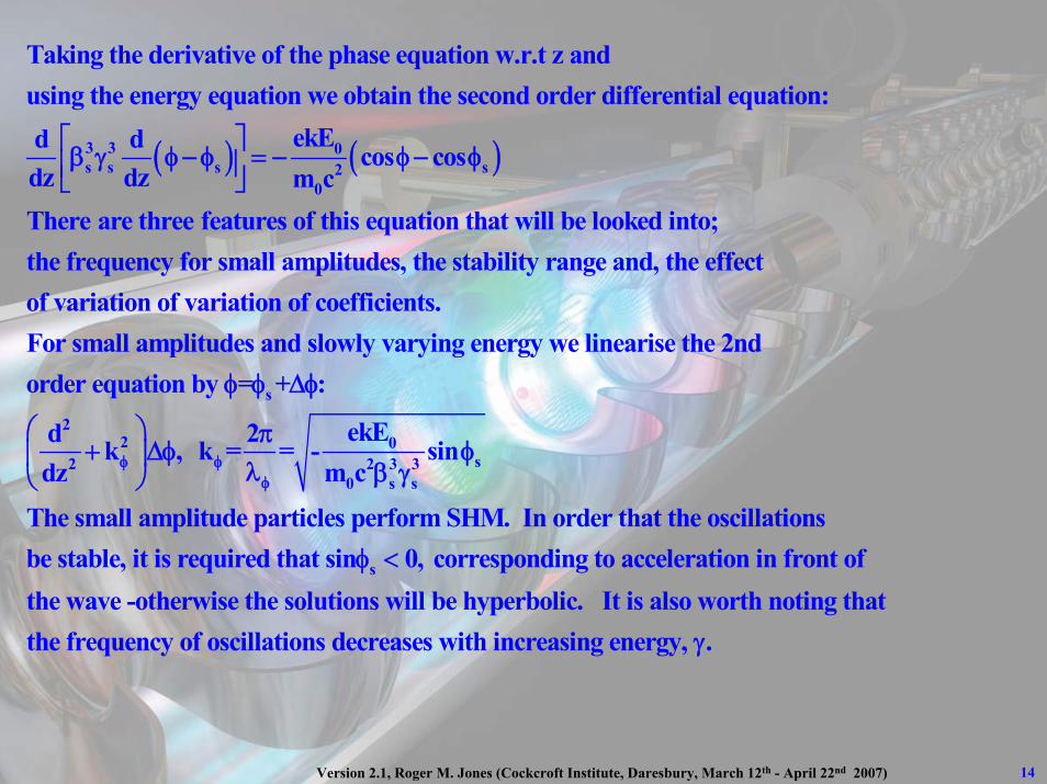
1 2Q (z)Replacing dt dz dz in the E-field equation allows the v (z)

integral to be evaluated:ri(s)E(z,s) E(0,s)e 1-e2sQ

The energy gain of a synchronous particle passing through the accele

α= =

ω

ω ⎡ ⎤= − ⎣ ⎦

( )

z

z

L L

0 0

( / Q)t-2

( / Q)tz-2

rator

is given by: V(t)= E(z,t)dz. Also, the Laplace transform: V(s)= E(z,s)dz

LUsing the previous expression for z= 1 e gives:1-e

Ldz= e dt1-e Q

Using this expession in the

− ωτ

− ω

τ

⎡ ⎤−⎣ ⎦

ω

∫ ∫

( ) ( ) ( )F

F F

(s / Q)t2 2

( / Q)t (s /Q)t

F z

E-field equation and integrating:E(0,s) L ri(s)LV(s) 1 e

1 e s /Q Q 2sQ 1 e

1 e 1 eQ(s / Q)

where t t (L) 2 Q/ is the filling time of the accelerator

− +ω

− τ − τ

− ω − +ω

ω ω⎡ ⎤= − −⎣ ⎦− + ω −

⎡ ⎤ω⎡ ⎤ ⎡ ⎤− − −⎢ ⎥⎣ ⎦ ⎣ ⎦+ ω⎣ ⎦= = τ ω section.


0

0 i

i 0

0

Now, let us assume that E(0,t) and i(t) are step functions:E(0,t)=E U(t)i(t) i U(t t )

where t is the time when the beam is injected, i is the average beamcurrent, E is the amplitude of the ele

⎧⎪⎨ = −⎪⎩

b

0 b

ctric field at z=0 and U(t) is theunit step function.

If there are N equally spaced bunches, each of charge q, and the bunchtrain has a time span t , the average current can be expessed as:i Nq/ tNow,

=

i

i i zz

0st

0

st -s(t t )-st0 0

2 2

we can readily obtain the Laplace tranform of the field and current:E(0,s)=E / s

i(t) (i / s)e

This enables the E-field and energy gain to be evaluated:

E ri e eE(z,s) e -s 2Q s s

−

− +

⎧⎪⎨

=⎪⎩

ω= −

⎡ ⎤⎢ ⎥⎣ ⎦


( ) ( )i

F

F

stst20 0

22

st22

E L ri e LV(s) 1 e e

2Qs1 e s /Q sQ

1 1 e e(1 e )(s /Q)Q

Taking the inverse Laplace transform gives the E-field at any pointand the energy gain as a function of time

−−− τ

− τ

−− τ− τ

ω ω⎡ ⎤= − −⎣ ⎦− + ω

⎡ ⎤ω ⎡ ⎤− −⎢ ⎥⎣ ⎦− + ω⎣ ⎦

( ) ( )

}

f

i

00 z i i i z i

( / Q)t 20 0

2 2

( / Q)(t t )f

20

i2 2

( / Q)(t t )i

:ri

E(z,t) E U(t t ) (t t )U(t t ) (t t t )U(t t )2Q

E L 1 e E LeV(t) U(t)

1 e 1 e

1 e U(t t )

ri L Le L(t t )2 Q(1 e ) (1 e )

1 e U(t t )

r

− ω − τ

− τ − τ

− ω −

− τ

− τ − τ

− ω −

ω= − − − − + − − −⎡ ⎤⎣ ⎦

⎡ ⎤−⎣ ⎦= −− −

⎡ ⎤− −⎣ ⎦⎧ ω⎪+ − −⎨

− −⎪⎩

⎡ ⎤− −⎣ ⎦

−2 2

0i F i f i F2 2

i Le Le(t t t ) 1 (t t t ) U(t t t )2 QQ(1 e ) (1 e )

− τ − τ

− τ − τ

⎧ ⎫ω ω⎡ ⎤⎪ − − − − − − − −⎨ ⎬⎢ ⎥− −⎪ ⎣ ⎦⎭⎩


Having obtained these general expressions, let us now apply them to some practical examples.

The first example is for the case where the beam is injected exactly after one RF filling time. Most of the traveling-wave linear accelerators work in this mode.

The second example is for the case where beam injection takes place before the RF structure is entirely filled up. The linear colliders accelerating multi-bunches will work in this mode.

Beam Injection after one Filling TimeBeam Injection after one Filling TimeIn this case, for convenience we choose the time at which the beam is turned on as zero. The new time then starts after one filling time:

2t /Q0

0 f2 2

20

0 f2

-2 1/2 1/20 in

ri Le LE L t (1 e ) 0 t t2 Q(1 e ) (1 e )

V(t)ri L 2reE L 1 t t

2 (1 e )

where E L=(1-e ) (P rL)

− τ−ω

− τ − τ

− τ

− τ

τ

⎧ ⎡ ⎤ω+ − − ≥ ≤⎪ ⎢ ⎥− −⎪ ⎣ ⎦= ⎨

⎡ ⎤⎪ − − ≥⎢ ⎥⎪ −⎣ ⎦⎩


Transient Beam Loading for Injection before t=tF and at t=tF


F

f

2 t / Q0b 0 2

2 (t / t )202

F

b

The transient beam loading for 0 t t can be expressed as:ri L

V V(t) E L 1 e t eQ2(1 e )

ri L t1 2 e et2(1 e )

What happens to the derivative of V at the

− τ −ω− τ

− τ− τ− τ

≤ ≤

ω⎡ ⎤Δ = − = − −⎢ ⎥− ⎣ ⎦

⎡ ⎤⎛ ⎞= − τ −⎢ ⎥⎜ ⎟

− ⎢ ⎥⎝ ⎠⎣ ⎦Δ

F

b 0loss t 0

t 0

loss

F

beginning of beam injection (t t )?

d V i r L2k q/ t

dt 2QrL Rwhere the energy loss factor is given by: k

4Q 4Q(r R/ L).Also, what occurs at time t after the beam has been turned on?A

==

≤

Δ ω= − = Δ Δ

ω ω= =

=

F

b

t 0

fter t :

d V0

dtThis corresponds to the transition from transient to steady state beamloading.

=

Δ=


Early Injection for Early Injection for Multibunch Multibunch OperationOperation

In order to increase the luminosity and RF energy transfer efficiency of a linear collider, multi-bunch operation will almost certainly be required.

The beam should then be injected before the accelerator section is completely filled so that to first order, the energy decrease due to beam loading is compensated by the energy increase due to filling.

Homework. For a bunch train consisting of bunches spaced by ΔS from their neighbours show that the energy compensation condition andmaximum energy sag are given by:

lossF

0 loss

2max loss2

F

2qk / LctSL L E Nqk / L

1V N k q Sct2(1 e )− τ

Δ ⎛ ⎞= ⎜ ⎟ +⎝ ⎠

⎛ ⎞τδ = − Δ⎜ ⎟

− ⎝ ⎠


• Sometimes useful to be able to calculate the loss factor of multiple identical cells in terms of the single-cell value.

• We will calculate the loss factor per unit length.• This is useful for part I of the computer project.

• N.B. here we will be analyzing multiple identical cells. This is of course quite different from the multi-cell loss factor calculated for cells with different dimensions (such as for detuned structures, which will be covered later).

• Loss factor is defined as:

• Where V is the voltage (from an integral of Ez along the axis) and U is the energy stored in the mode.

• For a single infinitely repeating cell of period

Multi-Cell Loss Factors in Terms ofSingle-Cell Loss Factors

Single-Cell Cavity

2

lossV

k4U

=> =

L

0V E(z)Exp(ikz)dz

where k / c.

=

= ω∫

*Take care not to confuse the wavenumber k with the loss factor (context should make it clear!).

Multi-Cell Cavity


• For a string of cavities with common period p the resonance condition is:=> E(z+L) = E(z)e-i φ (where φ is the phase advance over one cell).

• Thus, the voltage dropped across the complete cavity of N cells is:

• Here the phase slip angle has been defined as: δ = φ - ωp/c = φ - φacc ω/ ωacc.

Np p Npikz ikz ikz

0 0 (N 1)p

p pikz ik(z [N 1]p)

0 0i(N 1) i(N 1) p / c

0N 1

in( p / c)0

n 0

iN( p / c)

0 0i( p / c)

V E(z)e dz E(z)e dz ....... E(z)e dz

E(z)e dz ...... E(z [N 1]p)e dz

V [1 ....e e ]

V e

1 eV V1 e

−

+ −

− − φ − ω

−− φ−ω

=

− φ−ω−

− φ−ω

= = +

= + + −

= +

=

⎡ ⎤−= =⎢ ⎥−⎣ ⎦

∫ ∫ ∫

∫ ∫

∑

( )i N 1 / 2

220

NSin2

Sin2

1 CosNV V .1 Cos

− δ

δ⎛ ⎞⎜ ⎟⎝ ⎠

δ⎛ ⎞⎜ ⎟⎝ ⎠

− δ⎡ ⎤⇒ = ⎢ ⎥− δ⎣ ⎦


• In terms of the modulation index M we have:|V|2 = |V0|2M2

where:

• Taking the limit of the phase slippage going to zero then:

• i.e. the voltages add: V = NV0, as one might expect!

• Now we can calculate the LOSS-FACTOR PER UNIT LENGTH

• Here the relation U = NU0 has been used (i.e. the stored energy, U0, is independent of the phase factor φ).

NSin2M

Sin2

δ⎛ ⎞⎜ ⎟⎝ ⎠=

δ⎛ ⎞⎜ ⎟⎝ ⎠

{ }0

lim M Nδ→

=

2' 'loss 0 2

0'0

0

2

2

V1 Mk kNp 4U N

V1where kp 4U

=> = =

==


2' 'loss 0 acc2

acc

p0' i z / c0 0 0

0

2

M Sin(N / 2)k k ; M ; p / cSin( / 2)N

V1k ; V E(z)e dzp 4U

ω

δ ω= = δ = φ − ω = φ − φ

δ ω

== = ∫

Summary

• For example, consider 10 cells with φ= φacc and ω= ωacc => M=N • => k’loss = k’0 (single-cell and multi-cell loss factor per unit length are identical).• However, kloss = 10 k0 (the ten-cell loss factor is an order of magnitude larger

than the single-cell loss factor)


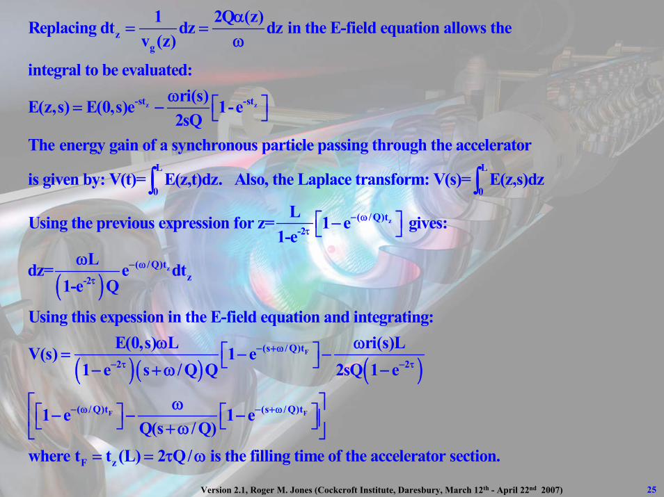
Motivation and Validation

The field of a point charge at rest is isotropic. The field of a charge moving relativistically is concentrated in a characteristic ‘pancake’. The angle subtended by the field shrinks to zero as particle becomes ultra-relativisitic –i.e. the velocity of the particle approaches the velocity of light.

In the limit of v->c the field is entirely perpendicular to the motion. In this case, The the radial field is given by:

0r 0

Z qE (r, z, ) Z H (r, z, ) exp( j z)

2 r cφ

ωω = ω = −

π

Coaxial Wire Measurement of Coaxial Wire Measurement of Loss Factor and WakeLoss Factor and Wake--Field Field


The amplitude of the field decays inversely with the radial distance away from the charge. This is also the case for a charge moving in a perfectly conducting pipe (with no obstructions present). In both cases the e.m. field travels with the charge.

Now consider a perfectly conducting cylindrical waveguide with a circular cross-section of radius b in which a wire of radius a has been inserted on-axis. The resulting coaxial structure allows the propagation of all frequencies. The TEM mode of this structure is given by:

where A is a constant depending on the power launched down the structure.

Thus, we can make an analogue of electron beam traveling down a structure by investigating the progress of the TEM field excited in a waveguide in which a centre conductor has been placed symmetrically within it.

r 0 0AE (r, z, ) Z H (r, z, ) Z exp( j z)r cφ

ωω = ω = −


Coaxial Measurement Wire Measurement of Loss Factor from a Lumped Equivalent Circuit Analysis

The equivalent circuit of the wire inserted into the Device Under Test (DUT) is illustrated below. The impedance Z represents that of the DUT and impedances either end are assumed to matched to the source.

We assume the generator and detector are matched to the source. The power available to the output Z0 is:

P0 = V2/(8Z0)

The transmission coefficient is given by:

Schematic illustrating DUT and S21 measurement

Equivalent circuit of DUT of impedance Z and matched input and output

20

0 0

Z VT i , where i = ,Z R jX2P 2Z Z

= = ++


2 20 0

02 2 20 0

0

4Z 4ZT , and at resonance: T = .

(2Z R) X (2Z R)We normalise the power with respect to the maximum power that can be transmitted to the output Z . Thus, the power dissipated in the DUT is:

P

=+ + +

2 2diss 0

2 20 0

0

0

02 2

0 02 2 2 2

0

R +4Z R+X1- T

P (R+2Z ) X

For a resonance in a parallel R-L-C we have:R

Z~ 2Q( - )

1+j

Thus, let =-tan and we have R=R /(1+ ) and X=-R /(1+ ).

Also, R X R /(1 )Now, the loss factor is

= =+

ω ωω

ξ ψ ξ ξ ξ

+ = + ξ

0 0 0 0 0 accloss 2mode

acc 0

2 2acc 0

given by:

R R R1 1k Rd d2Q 2Q 4Q1

Here, R 2R .

N.b. this R V / P and R V /(2P)

∞

−∞

ω ω ω= ω = ξ = =

π π + ξ

=

= =

∫ ∫


221

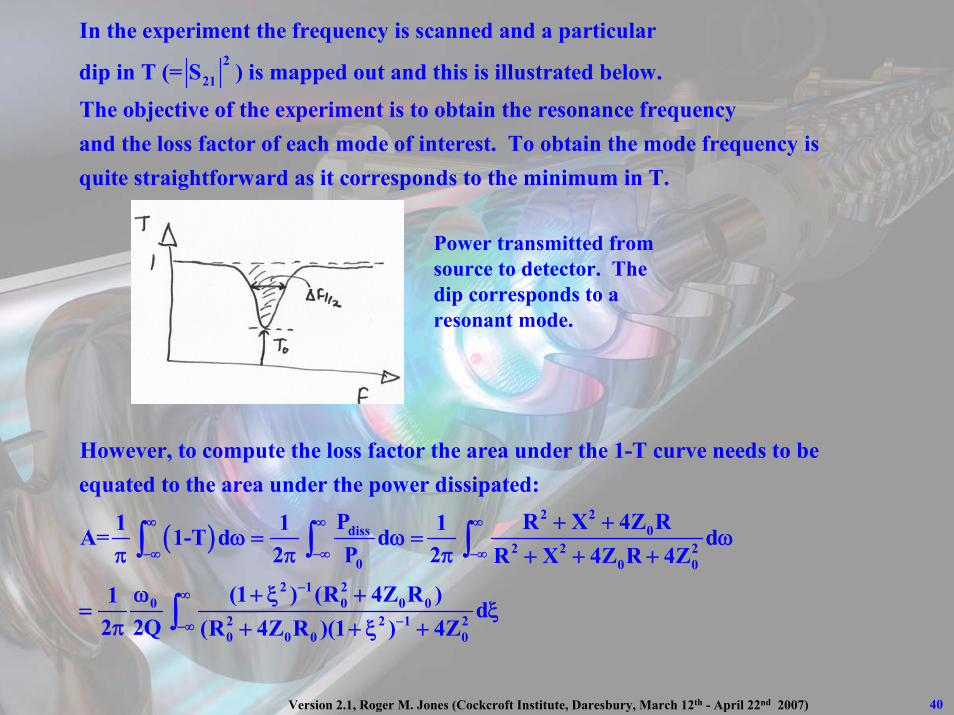
In the experiment the frequency is scanned and a particular

dip in T (= S ) is mapped out and this is illustrated below.

The objective of the experiment is to obtain the resonance frequency and the loss factor of each mode of interest. To obtain the mode frequency isquite straightforward as it corresponds to the minimum in T.

However, to compute the loss factor the area under the 1-T curve needs

( )2 2

diss 02 2 2

0 0 02 1 2

0 0 0 02 2 1 20 0 0 0

to be equated to the area under the power dissipated:

P R X 4Z R1 1 1A= 1-T d d d2 P 2 R X 4Z R 4Z

(1 ) (R 4Z R )1 d2 2Q (R 4Z R )(1 ) 4Z

∞ ∞ ∞

−∞ −∞ −∞

−∞

−−∞

+ +ω = ω = ω

π π π + + +

ω + ξ += ξ

π + + ξ +

∫ ∫ ∫

∫

Power transmitted from source to detector. The dip corresponds to a resonant mode.


2

20 0 0 0

2 2 20 0 0

0 0 0 0 0 0 0

0 0 0 0 0 020 0 0

0 020 00 0

loss

multiplying the numerator and denominator by (1 ):(R 4Z R )

A= d4 Q (R 2Z ) 4Z

R R 4Z R 4Z( )

4 Q 2Z R 2Z 8Z Q R 2Z

4Z R 4ZHowever,T 1 T

R 2Z(2Z R )and we obtain:

k

∞

−∞

+ ξ

ω +ξ

π + + ξ

ω π + ω += =

π + +

+= ⇒ + =

++

ω=

∫

0 0

0

01/ 2 0

20

1/2

loss 0 1/ 2 0

0

R 4ZA

2Q 1 T

1-TIf the dip is Lorentzian, i.e. 1-T= and A= f (1 T )

f-f 21+(2 )f

k 2 Z f (1 T )

Thus, in the experiment all we are required to do is measure theminimum transmission (T ), t

=+

πΔ −

Δ

⇒ = π Δ −

he half power points of the mode andthe loss factor is readily calculated.


The longitudinal wake of a particular mode is calculated according to:Wz(s)=2kloss,0cos(ωos/c). The complete wake-field is obtained by summing over all such modes.

For the transverse modes, the dipole is the most critical. The dipole wake is computed according to:

where r is the offset of the driving bunch, a0 is the position at which the loss factor is calculated, ωd/(2π) is dipole mode frequency and kloss,d is the dipole mode loss factor. Again, we sum over all modes to obtain the complete field.

,

loss,d 0t d

0

2k r / aW (s) sin( s / c)

( a / c)= ω

ω


Wire Measurement of Impedance: Formally Exact Method

The basis of the method is to take a transmission line and embed the coupling impedance with it. The goal of the analysis being to uncover the embedded impedance in terms of the measured experimental parameters –S matrix parameters.

We begin with the standard unperturbed transmission line. Here we consider a series impedance Z (=R0+j ωL0) and a parallel admittance Y (=jωC0).

0 00

0

00 0 0 0 0

0 0

The characteristic impedance of the line is given by:

R j LZZY j C

and the propagation constant:jR

= (R j L )j C ~ L C2 L C

andthis means the transmission scattering matrix component is given by:

+ ω= =

ω

β + ω ω ω −

21S exp( j ) exp( j l), where l is the length of the transmission line= − θ = − β


Wire Measurement of Impedance: Formally Exact Method

Now we consider the DUT (Device Under Test) embedded within the transmission line as a coupling impedance. We consider the same transmission line with the same physical length, parallel admittance per unit length but with a series impedance per unit length which is a factor of ζ2 different.

This modified series impedance per unit length can be thought of the sum of the series impedance of the unperturbed line jβZ0, in series with an additional impedance per unit length Z///l=j β(ζ2 -1)Z0 -the coupling impedance. This is illustrated below.

In order to calculate this coupling impedance in terms of the measured scattering parameters we need to transform the Z-matrix for the transmission line to the S-matrix

Transmission line with an embedded coupling impedance Z//.


1 111 12

21 222 2

0

0

The impedance matrix for a transmission line is defined as:V IZ Z

Z ZV I

and for the transmission line DUT:cos 1-j Z

Z=1 cossin Z

The S-matrix is related to the Z-matr

⎛ ⎞ ⎛ ⎞⎛ ⎞=⎜ ⎟ ⎜ ⎟⎜ ⎟

⎝ ⎠⎝ ⎠ ⎝ ⎠

ξθξ ⎛ ⎞⎜ ⎟ξθξ ⎝ ⎠

10 0 0

2 2 20 0

0

ix according to:S=(Z-Z U)(Z+Z U) , where U=Identity matrix and Z is thereference impedance (originally matched out with the reference device).Thus, the S-matrix becomes:

Z ( 1)sin 2j Z2j Z

S=

−

ξ − ξθ − ξ− ξ 2 2 2

02 2 20 0

11

21,DUT

Z ( 1)sinZ ( 1)sin 2jZ cos

Thus the transmission matrix is given by:

jS cos ( )sin2

−−

⎡ ⎤⎢ ⎥

ξ − ξθ⎣ ⎦ξ + ξθ − ξ ξθ

⎡ ⎤= ξθ + ξ + ξ ξθ⎢ ⎥⎣ ⎦


21,REF

j21,DUT

121,REF

and as the reference tranmission is given by:S exp( j ) then :

S ejS cos ( )sin2

No approximations have been made up to this stage.

θ

−

= − θ

=ξθ + ξ + ξ ξθ

Clearly if the reference line has the same impedance as the DUT then ξ=1 and S21 = exp(-jθ).

Taking the natural log of the S21 ratio, with some rearrangement, leads to:

This formula can be solved numerically but in the process of performing experiments it is useful to have analytical expressions. Thus, we explore several approximate formula for the impedance.

( )21,DUT2 2j 2

21,REF

S 4log j logS ( 1) e ( 1)− ξθ

⎛ ⎞ ⎡ ⎤ξ= − ξ − θ +⎜ ⎟ ⎢ ⎥⎜ ⎟ ξ + − ξ −⎣ ⎦⎝ ⎠


z 0 z 0

z 0

21,DUTz

0 21,REF

1. log formula

Substitute for in terms of Z / Z : 1 jZ /(Z ) and expand

in powers of Z / Z :

SZ2log

Z S

This is valid for a small coupling impedance compared to the unperturbed(ref

−

ξ ξ = − θ

⎛ ⎞− ⎜ ⎟⎜ ⎟

⎝ ⎠

z 0

21,DUT 2

21,REF

21,DUT 21,DUTz

0 21,REF 21,REF

erence) characteristic impedance Z / Z 1

2. Improved log formulaRetain and make an expansion in -1:

Slog j ( 1) ( 1)

S

S SZ j2log 1 logZ S 2 S

<

ξ ξ

⎛ ⎞= − θ ξ − + θ ξ −⎜ ⎟⎜ ⎟

⎝ ⎠

⎛ ⎞ ⎛⇒ = − +⎜ ⎟⎜ ⎟ θ⎝ ⎠ ⎝

z 0

Both the log and the improved log formula are first order power series

expansions. The improved formula includes a expansion as -1= 1-jZ /(Z ) 1.

It is equivalent to neglecting the mis

⎡ ⎤⎞⎢ ⎥⎜ ⎟⎜ ⎟⎢ ⎥⎠⎣ ⎦

θ ξ θ −

j21,DUT

match at the beginning and end of the transition (prove this!), i.e. S ~ e− ξθ


jθ21,DUT

z 0-121,REF

21,DUT

z21,REF

0

21,REFz 0

21,

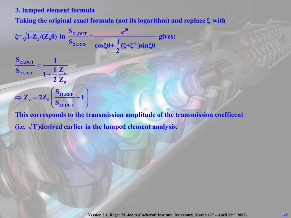
3. lumped element formulaTaking the original exact formula (not its logarithm) and replace with

S eξ= 1-Z /(Z θ) in = gives:jS cosξθ+ (ξ+ξ )sinξθ2

S 1Z1S 1

2 Z

SZ 2Z

S

ξ

=+

⇒ =DUT

1

This corresponds to the transmission amplitude of the transmission coefficent

(i.e. T)derived earlier in the lumped element analysis.

⎛ ⎞−⎜ ⎟⎜ ⎟

⎝ ⎠


Domain of applicability

For longer cavities (structures long compared to wavelength) the improved formula is the most appropriate one to use. The improved formula is often significantly more accurate than the log formula.

Use of either log formula for short structure can easily give inaccurate results. Use the lumped in this case as it is the most appropriate one for this system.


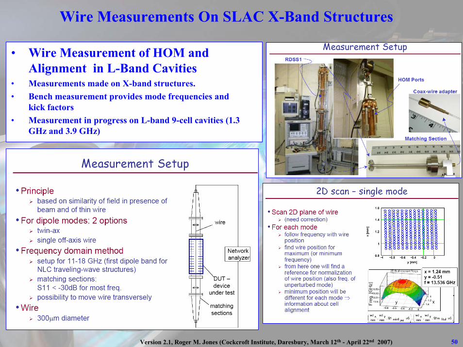
• Wire Measurement of HOM and Alignment in L-Band Cavities

• Measurements made on X-band structures.• Bench measurement provides mode frequencies and

kick factors• Measurement in progress on L-band 9-cell cavities (1.3

GHz and 3.9 GHz)

Wire Measurements On SLAC X-Band Structures


S11 (linear)

0

0.1

0.2

0.3

0.4

0.5

0.6

0.7

0.8

0.9

1

2 3 4 5 6 7 8 9

Frequency (GHz)

S11

On-axis1mm Off-axis2mm Off-axis3mm Off-axis4mm Off-axis

Frequency Domain S11 Simulations for Several Wire Offsets

Frequency DomainWire Measurements of Crab Cavities

Resonances located at dipole modesArea under S21 ~ Zl (beam impedance)Fourier transform enables wake-field and kick factors to be calculatedBench-top measurement allows rapid determination of cavity modes (sync. freqs and

kick factors).Also allows cavity alignment to be determined.Use method to determine modes in main linac cavities (1.3 GHz)

Crab Cavity Measurement Set-Up

Documents

Linear Accelerators: Theory and Practical Applications: …atlas.physics.arizona.edu/~kjohns/downloads/linac/Linacs_Week_4... · Linear Accelerators: Theory and Practical Applications: