Embed Size (px)
Citation preview
Ninth International Conference on
Computational Fluid Dynamics (ICCFD9),
Istanbul, Turkey, July 11-15, 2016
ICCFD9-xxxx
Linear and Nonlinear Based Ship Motion of a Naval Combatant
Model
Ferdi Cakici*, Omer F. Sukas, Omer K. Kinaci, Ahmet D. Alkan
1Yildiz Technical University Faculty of Naval Architecture and Maritime, Istanbul, Turkey
Corresponding author: [email protected]
Abstract: Seakeeping is a very complex problem in Maritime problems involving at
least 3 degree-of-freedom (3-DOF) motion of the hull and until commercialized CFD
softwares became widely used, the problem was approached by linear approaching
applying potential theory. With this motivation, two kinds of numerical methods are
employed to study the vertical motions for one encounter frequency where
experimental results are available in the literature. While the first method is widely
known linear “strip theory”, the other one is the fully non-linear U-RANS solver.
DTMB 5415 ship form is selected for the computational work. In the first method,
the hydrodynamic coefficients in the motion equations are determined and ship
responses are found. In the second method, ship responses are found by solving
Newton’s Motion Law after calculating forces/moments acting on the ship hull via
the FVM (Finite Volume Method). Computational study is carried out for Fn=0.41
only. Results are validated with experiments and comparisons are made between the
two numerical approaches.
Keywords: Seakeeping, Strip Theory, URANS, ship motions
1 Introduction
Investigation of ship motions in waves is one of the most challenging topics in the field of
hydrodynamics. The difficulties originate the nature of seakeeping calculations because waves are
playing a significant role on the ship’s response. Viscous flows are highly nonlinear and the Reynolds
numbers covered in ship motions are usually high in which turbulent effects are unavoidable. Gravitation
complicates the problem even more because waves in nature are not in sinusoidal form as in regular
waves. Additionally, the complex geometry of ship hulls majorly affect the restoring terms in the
equations of motion. Linear theory regards the restoring terms as constant and this approach fails
especially at higher wave amplitudes.
URANS equations which are discretized with the Finite Volume Method are introduced to obtain 6DOF
motion of a ship in regular and irregular waves. The inclusion of viscosity with several turbulence
models in this approach increases the robustness of the method and its applicability in many cases.
Salvesen et al. presented the original strip theory by using 2-D hydrodynamic coefficients which are
obtained by Frank’s method [1, 2]. With the strip theory, it was possible to get transfer functions for
vertical motions of any 3-D ship form in regular waves. Strip theory is currently a common method to
perform seakeeping analyses of a ship and there are many studies implementing the theory.
Beck and Reed advises that the best option to solve for maritime problems are 3D URANS methods [3].
Sato et al. studied on coupled vertical motions for Wigley and Series 60 hull forms at head waves. They
compared their results with experimental data. They concluded that CFD analyses are in good
accordance with experiments for the Wigley hull but not Series 60 hull form [4]. Weymouth et al. also
carried out seakeeping simulations by implementing URANS. Their results are compatible with
experiments and they advised the best methods to be implemented in a wide Froude number range [5].
However, in this study the motions are investigated only for a low wave slope range. High wave slope
ranges are investigated by Deng et al. and they investigated the vertical motions of a benchmark
container ship form. Their study also included numerical uncertainty analyses [6]. Bhushan et al.
performed seakeeping analyses for both the model and the full scale of DTMB 5415 ship hull. They also
predicted maneuvering derivatives for full scale hull [7]. Simonsen et al. prepared a comprehensive
study by using URANS for many different types of ships for seakeeping calculations [8, 9]. Wilson et
al. carried out CFD simulations to obtain TF’s of vertical responses of the S-175 ship in regular head
waves [10].
In this study, as a first step, the ship resistance computations are carried out in calm water and compared
with experimental data. Then, Salvesen’s strip theory is used to obtain pitch and heave responses for
one encounter frequency which is accepted to be around resonance region. Finally, FVM which enables
to discretize the URANS equations is used to obtain the pitch and heave responses of the hull.
2 Geometric Features and Physical Conditions
In this study, a 1/24.83 scaled model of the DTMB 5415 hull given by Figure 1 is used for numerical
simulations. The experimental results are given in the reference report [11]. The main particulars of the
model hull are given in Table 1. All values are presented for the static case. The numerical simulations
were performed for the bare hull case only without any appendages.
Table 1. Main particulars of the model
Figure 1: 3D representation of the DTMB 5415 INSEAN Model.
Main parameters Units Value
LWL m 5.720
BWL m 0.768
T m 0.248
LCG (from aft) m 2.924
Displacement kg 549.0
Iyy kg
∗ m2
1123.2
V m/s 3.07
Fr - 0.41
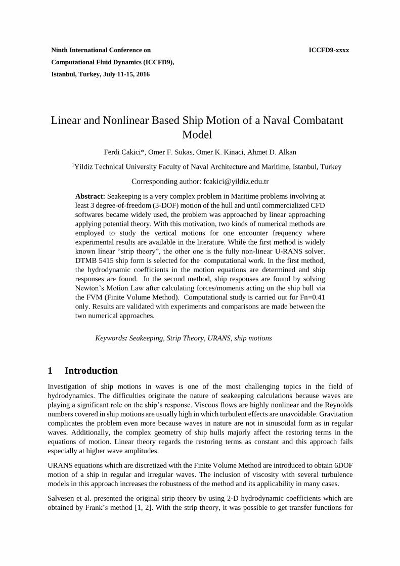
Figure 2: Schematic physics.
An Earth-fixed Cartesian coordinate system 𝑥𝑦𝑧 is selected for the solution domain. 𝑥𝑦 plane represents
the calm free water surface and 𝑧 is defined as the vertical axis. The model is moving in the positive x
direction with 2DOF including heave and pitch motions only as indicated in Figure 2. A new local
coordinate system is created for the ship to obtain 2DOF motion. The URANS and strip theory
calculations were performed at 𝜔= 2.488 rad/s and Fn=0.41 as shown in Table 2. All calculations are
performed at regular head waves.
Encounter frequency for head waves is defined as below:
𝜔𝑒 = 𝜔 + (𝜔2
𝑔𝑉) (1)
where 𝑔 denotes gravity, 𝜔 denotes frequency of the wave, 𝑉 denotes velocity of the ship in Equation
1. Small amplitude waves (𝐴 ∗ 𝑘 = 0.025) are selected for numerical simulations to be consistent with
the experimental procedure [11] where 𝐴 denotes the wave amplitude and 𝑘 denotes the wave number.
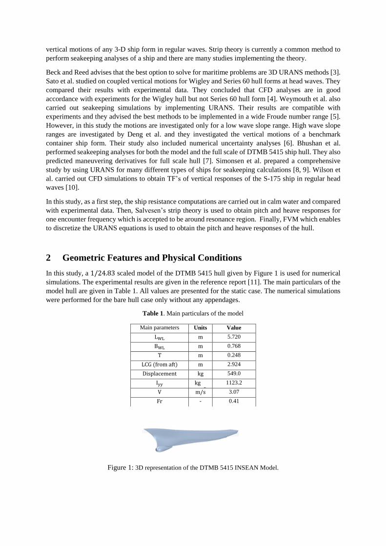
The generated regular wave for case 2 is given in Figure 3.
Table 2: Defined Cases for strip theory and URANS Calculations
Case
no. Methods Fn (-) A*k ω (rad/s)
ωe
(rad/s) λ/Lwl (-) H/λ (-) Time step size
0 URANS 0.41 N/A N/A N/A Calm water N/A 0.005*V/LWL
1 Strip Theory
adadafgfddd
and
URANS
0.41 - 2.488 4.427 1.740 - -
2 URANS 0.41 0.025 2.488 4.427 1.740 1/125 Te/29
Figure 3: Regular wave representation for case 6 (5th-order Stokes waves).
3 Salvesen’s Strip Theory (ST)
In this theory, heave, pitch, sway, roll and yaw motion is predicted for a ship advancing constant speed
with arbitary heading in regular waves. Frank-Close Fit method is used to determine hydrodynamic
coeeficients in the equation. The 6DOF equation of motions which are based on Newton’s second law
of dynamics are given Eq.2. Since ship is symmetric, the equations are reduced two uncoupled sets
which are vertical and transversal. In a right-handed co-ordinate system, taking the origin to the ship’s
centre of gravity, these equations are compiled as below [2]:
6
1
( )ij ij j ij j ij j i
j
M A x B x C x F
(2)
for i=1,2…6
where i=1,3,5:Coupled surge, heave and pitch motions (vertical)
i=2,4,6: Coupled sway,roll and yaw motions (transversal)
jxAcceleration of harmonic oscilation in direction j
jxVelocity of harmonic oscilation in direction j
jxDisplacement of harmonic oscilation in direction j
iF Harmonic exciting wave force or moment in direction i
ijMSolid mass or inertia coefficient
ijAAdded mass or inertia coefficient
ijBDamping coefficient
ijCRestring coefficient
In this study, only vertical motions of the ships are considered and surge motion is neglected because
surge amplitudes are very small compared to heave and pitch motions.With only vertical 2DOF
assumption, one can express differential form of equation of vertical motion as Eq.3 and Eq.4.
3
33 3 33 3 33 3 35 5 35 5 35 5 3eiw t
M A x B C x A x B C xx ex F
(3)
5
5 55 55 55 55 55 5 53 3 53 3 53 3 5eiw t
I A x B x C A x B x C Fx x e
(4)
For head waves and two ship speeds, solution of these differential equation sets gives heave and pitch
amplitudes and phases for varying encounter frequencies and it allows to draw RAO graphs for both
vertical motions. According to Salvesen’s strip theory, heave added mass can be calculated as follows:
33 33 332
0
L
AUA a dx b
(5)
33 33 33
0
L
Ab dxB Ua (6)
The calculation of other coefficents can be found in Salvesen’s paper [2].
4 URANS EQUATIONS AND MODELING
The averaged continuity and momentum equations can be written for incompressible flow in cartesian
coordinates and tensor form as indicated Equation 7 and 8:
(7)
0i
i
U
x
( )( )
i i
j
i i
i j
i
j j
u uF
x
U U PU
x xt x
(8)
where ij are the mean viscous stress tensor components and shown in Equation 9.
( )i i
ij
j i
U U
x x
(9)
In this paper, two equation 𝑘 − 𝜀 turbulence model is used to include the effects of viscosity as it is
considered to be one of the most commonly used turbulence model for industrial applications [12]. The
employed solver uses a finite volume method which discretizes the Navier–Stokes (N-S) equations for
numerical model of fluid flow. Segregated flow model is used in the URANS solver and convection
terms in the URANS equations are discretized by applying second order upwind scheme. In the analyses,
the URANS solver runs a predictor–corrector SIMPLE-type algorithm between the continuity and
momentum equations. A first-order temporal scheme is applied to discretise the unsteady term in the N-
S equations. The free surface is dependent on the regular wave properties using Volume of Fluid (VOF)
model. In this model, computations are performed for water and air phases. Mesh structure and mesh
number in the free surface are significantly important to capture VOF profile accurately and second
order convection scheme is used to present results calculated by VOF more precisely. It is also should
be noted that all the analyses are performed in deep water conditions.
DFBI (Dynamic Fluid Body Interaction) module in the commercial software STAR CCM+ is used for
the motion of body which is free to heave and pitch. The 2DOF motion of the body is obtained by
calculating the velocity and pressure field in the fluid domain. For this purpose linear and angular
momentum equations, given in Equations 10 and 11 respectively, are solved:
F ma (10)
G G a GM I I (11)
where 𝐹denotes the total force, 𝑚 the mass, 𝑎 the acceleration, 𝑀𝐺 the moment taken from the center of
gravity, 𝐼𝐺 the inertial mass moment, 𝛼𝑎the angular acceleration and 𝜔 is the angular speed.
4.1 Selection of time step size
Explicit methods require higher computer memory due to the relatively larger fluid domain demanded
by the flow physics of ship hydrodynamic problems. Therefore implicit method is chosen for numerical
solution. In the explicit method, CFL condition has to be satisfied for the stability of the method.
However in the unsteady implicit problems, the restriction by the CFL condition is not an issue anymore
and it relaxes the computer in terms of memory. Time step size is selected as 1/29 of 𝑇𝑒for seakeeping
analyses which is more accurate than the value recommended by ITTC [13]. Here 𝑇𝑒 denotes encounter
period. For calm water resistance predictions, on the other hand, the authors stood by ITTC’s
recommendation time step size is selected to be 0.005 ∗ 𝐿𝑊𝐿/𝑉 [13].
4.2 Computational domain and boundary conditions
The boundary and initial conditions must be suitable for all numerical and analytical problems to have
a well posed problem. These conditions must be usually defined in accordance with the characteristics
of the flow. In this study, the computational domain was created in order to simulate the seakeeping
behavior of the naval surface combatant in regular waves. The rigid body motion approach was used for
representing coupled heave and pitch motions of the ship.
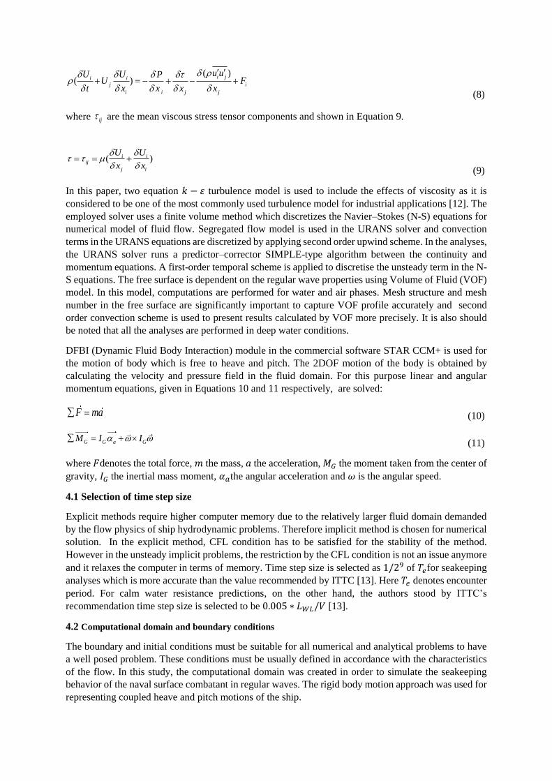
Only half of the body is modeled to decrease the domain size and so computational time. The boundary
conditions are shown in Figure 5.
Figure 5: Boundary conditions in the computational fluid domain.
5th-order Stokes waves are used to represent the wavy environment for all URANS analyses as they are
shown in Figures 3.
4.3 Mesh structure
The trimmed mesh module in the STAR CCM+ provides an efficient and secured method to generate
high quality grid for complex bodies like marine vehicles [14]. The trimmed mesh is mostly hexahedral
mesh with a minimal cell skewness.
As it can be seen from Figure 6, the grid system applied in CFD calculations are part of two blocks
which are overset and background regions. The background grids are fixed to global coordinate system
but the overset grids are moving with the body. The information is passed through the overlap block
between overset and background regions. With the overset grid system, any mesh modification or
deformation is not necessary which provides great flexibility over the other standard meshing
techniques.
The computational domain extends for 1.2L in fro nt of the overset region, 4.8L behind the overset
region, and 3L to the side and 2.5L under the boundries of overset region. The air region is 1L above
the overset region. The mesh is then refined at five different regions; overset, overlap, vicinity of the
hull, around free surface and Kelvin wake regions. Refinement blocks are also built near the ship’s bow
and stern regions in order to represent pitch motion well. Overlap region ensures the flow of information
between overset and backround regions. Three different unstructured hexahedral mesh system are
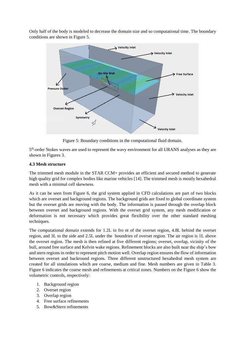
created for all simulations which are coarse, medium and fine. Mesh numbers are given in Table 3.
Figure 6 indicates the coarse mesh and refinements at critical zones. Numbers on the Figure 6 show the
volumetric controls, respectively:
1. Background region
2. Overset region
3. Overlap region
4. Free surface refinements
5. Bow&Stern refinements
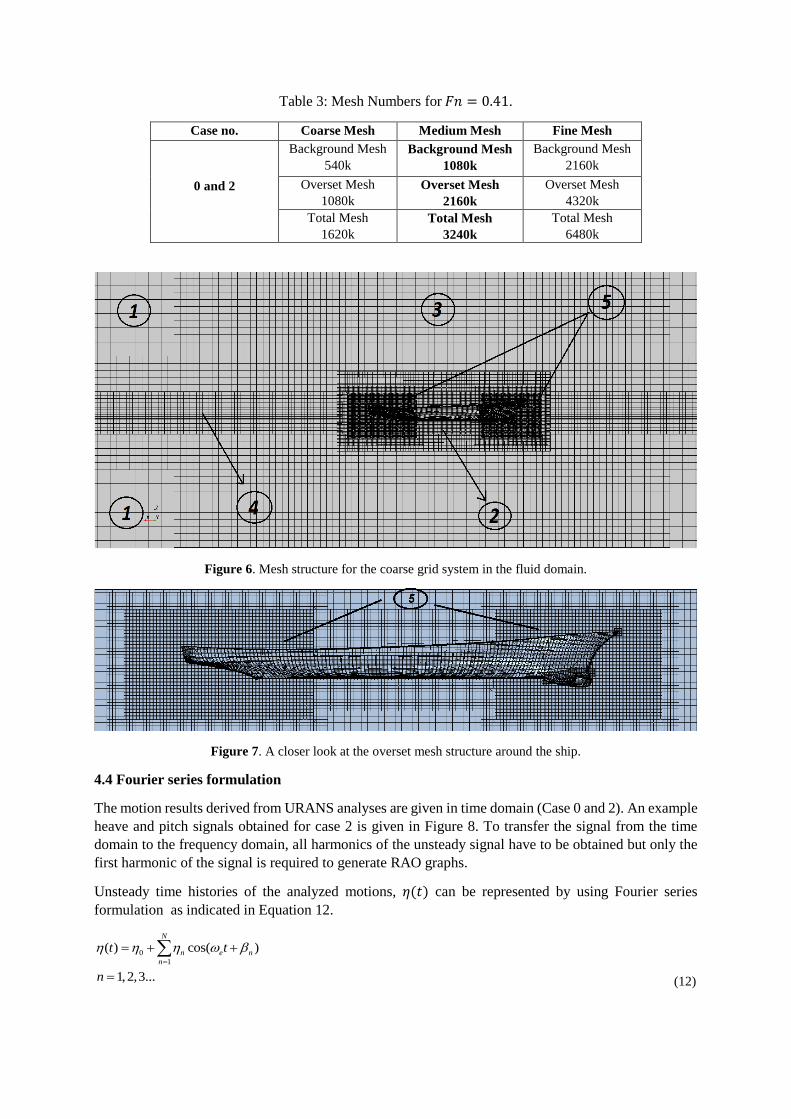
Table 3: Mesh Numbers for 𝐹𝑛 = 0.41.
Figure 6. Mesh structure for the coarse grid system in the fluid domain.
Figure 7. A closer look at the overset mesh structure around the ship.
4.4 Fourier series formulation
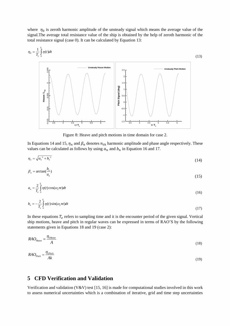
The motion results derived from URANS analyses are given in time domain (Case 0 and 2). An example
heave and pitch signals obtained for case 2 is given in Figure 8. To transfer the signal from the time
domain to the frequency domain, all harmonics of the unsteady signal have to be obtained but only the
first harmonic of the signal is required to generate RAO graphs.
Unsteady time histories of the analyzed motions, 𝜂(𝑡) can be represented by using Fourier series
formulation as indicated in Equation 12.
0
1
( ) cos( )
1,2,3...
N
n e n
n
t t
n
(12)
Case no. Coarse Mesh Medium Mesh Fine Mesh
0 and 2
Background Mesh
540k
Background Mesh
1080k
Background Mesh
2160k
Overset Mesh
1080k
Overset Mesh
2160k
Overset Mesh
4320k
Total Mesh
1620k
Total Mesh
3240k
Total Mesh
6480k
where 𝜂0 is zeroth harmonic amplitude of the unsteady signal which means the average value of the
signal.The average total resistance value of the ship is obtained by the help of zeroth harmonic of the
total resistance signal (case 0). It can be calculated by Equation 13:
0
0
1( )
eT
e
t dtT
(13)
Figure 8: Heave and pitch motions in time domain for case 2.
In Equations 14 and 15, 𝜂𝑛 and 𝛽𝑛 denotes 𝑛𝑡ℎ harmonic amplitude and phase angle respectively. These
values can be calculated as follows by using 𝑎𝑛 and 𝑏𝑛 in Equation 16 and 17.
2 2
n n na b (14)
arctan( )n
n
n
b
a
(15)
0
2( )cos( )
eT
n e
e
a t nt dtT
(16)
0
2( )sin( )
eT
n e
e
b t nt dtT
(17)
In these equations 𝑇𝑒 refers to sampling time and it is the encounter period of the given signal. Vertical
ship motions, heave and pitch in regular waves can be expressed in terms of RAO’S by the following
statements given in Equations 18 and 19 (case 2):
1Heave
HeaveRAOA
(18)
1Pitch
PitchRAOAk
(19)
5 CFD Verification and Validation
Verification and validation (V&V) test [15, 16] is made for computational studies involved in this work
to assess numerical uncertainties which is a combination of iterative, grid and time step uncertainties
t / Te
He
ave
/L
pp
3.5 4 4.5 5 5.5 6-0.0
15
-0.0
1-0
.00
50
0.0
05 Unsteady Heave Motion
t / Te
Pitch
Sig
na
l(d
eg
)
3.5 4 4.5 5 5.5 6-1.5
-1
-0.5
0
0.5
1
1.5
2
2.5Unsteady Pitch Motion
(𝑈𝐼, 𝑈𝐺 , 𝑈𝑇 respectively). Simulation numerical uncertainty 𝑈𝑆𝑁, given in Equation 20:
𝑈𝑆𝑁 = √𝑈𝐼2 + 𝑈𝐺
2 + 𝑈𝑇2
(20)
The V&V study is made for 𝐹𝑛 = 0.41 and at a wave frequency of 𝜔 = 2.488. Iterative uncertainties
in all trials are found to be very low when compared with grid and time step uncertainties; therefore, it
is assumed that 𝑈𝐼 ≈ 0. The element numbers for grid uncertainty and time step sizes for time step
convergence study is given in Table 4.
Table 4. Element numbers and time step sizes involved in the uncertainty study.
G3 G2 G1
Element no. 750,000 1,500,000 3,000,000
T3 T2 T1
Time step
size Te/27 Te/28 Te/29
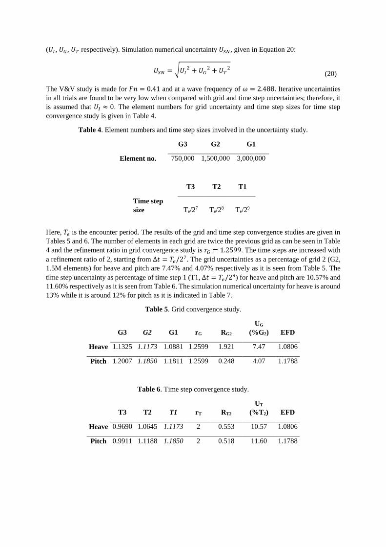
Here, 𝑇𝑒 is the encounter period. The results of the grid and time step convergence studies are given in
Tables 5 and 6. The number of elements in each grid are twice the previous grid as can be seen in Table
4 and the refinement ratio in grid convergence study is 𝑟𝐺 = 1.2599. The time steps are increased with
a refinement ratio of 2, starting from ∆𝑡 = 𝑇𝑒/27. The grid uncertainties as a percentage of grid 2 (G2,
1.5M elements) for heave and pitch are 7.47% and 4.07% respectively as it is seen from Table 5. The
time step uncertainty as percentage of time step 1 (T1, ∆𝑡 = 𝑇𝑒/29) for heave and pitch are 10.57% and
11.60% respectively as it is seen from Table 6. The simulation numerical uncertainty for heave is around
13% while it is around 12% for pitch as it is indicated in Table 7.
Table 5. Grid convergence study.
G3 G2 G1 rG RG2
UG
(%G2) EFD
Heave 1.1325 1.1173 1.0881 1.2599 1.921 7.47 1.0806
Pitch 1.2007 1.1850 1.1811 1.2599 0.248 4.07 1.1788
Table 6. Time step convergence study.
T3 T2 T1 rT RT2
UT
(%T2) EFD
Heave 0.9690 1.0645 1.1173 2 0.553 10.57 1.0806
Pitch 0.9911 1.1188 1.1850 2 0.518 11.60 1.1788
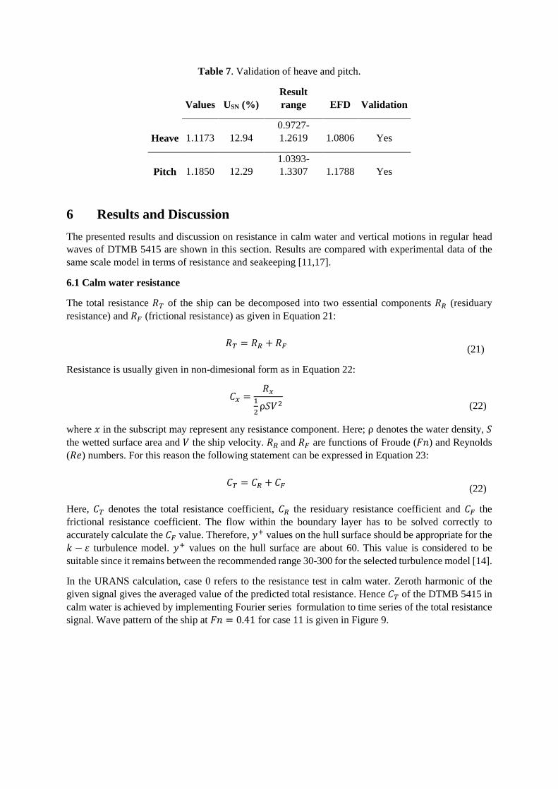
Table 7. Validation of heave and pitch.
Values USN (%)
Result
range EFD Validation
Heave 1.1173 12.94
0.9727-
1.2619 1.0806 Yes
Pitch 1.1850 12.29
1.0393-
1.3307 1.1788 Yes
6 Results and Discussion
The presented results and discussion on resistance in calm water and vertical motions in regular head
waves of DTMB 5415 are shown in this section. Results are compared with experimental data of the
same scale model in terms of resistance and seakeeping [11,17].
6.1 Calm water resistance
The total resistance 𝑅𝑇 of the ship can be decomposed into two essential components 𝑅𝑅 (residuary
resistance) and 𝑅𝐹 (frictional resistance) as given in Equation 21:
𝑅𝑇 = 𝑅𝑅 + 𝑅𝐹
(21)
Resistance is usually given in non-dimesional form as in Equation 22:
𝐶𝑥 =𝑅𝑥
1
2⍴𝑆𝑉2
(22)
where 𝑥 in the subscript may represent any resistance component. Here; ⍴ denotes the water density, 𝑆
the wetted surface area and 𝑉 the ship velocity. 𝑅𝑅 and 𝑅𝐹 are functions of Froude (𝐹𝑛) and Reynolds
(𝑅𝑒) numbers. For this reason the following statement can be expressed in Equation 23:
𝐶𝑇 = 𝐶𝑅 + 𝐶𝐹
(22)
Here, 𝐶𝑇 denotes the total resistance coefficient, 𝐶𝑅 the residuary resistance coefficient and 𝐶𝐹 the
frictional resistance coefficient. The flow within the boundary layer has to be solved correctly to
accurately calculate the 𝐶𝐹 value. Therefore, 𝑦+ values on the hull surface should be appropriate for the
𝑘 − 𝜀 turbulence model. 𝑦+ values on the hull surface are about 60. This value is considered to be
suitable since it remains between the recommended range 30-300 for the selected turbulence model [14].
In the URANS calculation, case 0 refers to the resistance test in calm water. Zeroth harmonic of the
given signal gives the averaged value of the predicted total resistance. Hence 𝐶𝑇 of the DTMB 5415 in
calm water is achieved by implementing Fourier series formulation to time series of the total resistance
signal. Wave pattern of the ship at 𝐹𝑛 = 0.41 for case 11 is given in Figure 9.
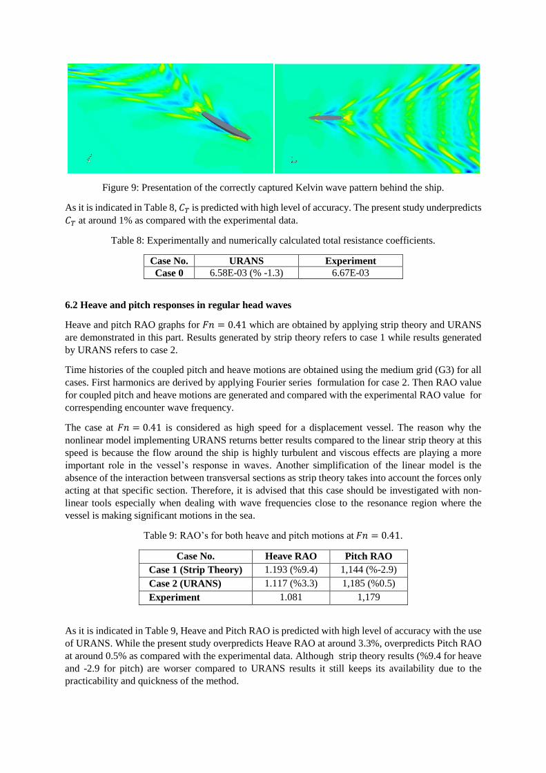
Figure 9: Presentation of the correctly captured Kelvin wave pattern behind the ship.
As it is indicated in Table 8, 𝐶𝑇 is predicted with high level of accuracy. The present study underpredicts
𝐶𝑇 at around 1% as compared with the experimental data.
Table 8: Experimentally and numerically calculated total resistance coefficients.
Case No. URANS Experiment
Case 0 6.58E-03 (% -1.3) 6.67E-03
6.2 Heave and pitch responses in regular head waves
Heave and pitch RAO graphs for 𝐹𝑛 = 0.41 which are obtained by applying strip theory and URANS
are demonstrated in this part. Results generated by strip theory refers to case 1 while results generated
by URANS refers to case 2.
Time histories of the coupled pitch and heave motions are obtained using the medium grid (G3) for all
cases. First harmonics are derived by applying Fourier series formulation for case 2. Then RAO value
for coupled pitch and heave motions are generated and compared with the experimental RAO value for
correspending encounter wave frequency.
The case at 𝐹𝑛 = 0.41 is considered as high speed for a displacement vessel. The reason why the
nonlinear model implementing URANS returns better results compared to the linear strip theory at this
speed is because the flow around the ship is highly turbulent and viscous effects are playing a more
important role in the vessel’s response in waves. Another simplification of the linear model is the
absence of the interaction between transversal sections as strip theory takes into account the forces only
acting at that specific section. Therefore, it is advised that this case should be investigated with non-
linear tools especially when dealing with wave frequencies close to the resonance region where the
vessel is making significant motions in the sea.
Table 9: RAO’s for both heave and pitch motions at 𝐹𝑛 = 0.41.
Case No. Heave RAO Pitch RAO
Case 1 (Strip Theory) 1.193 (%9.4) 1,144 (%-2.9)
Case 2 (URANS) 1.117 (%3.3) 1,185 (%0.5)
Experiment 1.081
1,179
As it is indicated in Table 9, Heave and Pitch RAO is predicted with high level of accuracy with the use
of URANS. While the present study overpredicts Heave RAO at around 3.3%, overpredicts Pitch RAO
at around 0.5% as compared with the experimental data. Although strip theory results (%9.4 for heave
and -2.9 for pitch) are worser compared to URANS results it still keeps its availability due to the
practicability and quickness of the method.
7 Conclusions
In the present paper, the coupled pitch and heave motions on regular head waves for one case were
investigated with linear and nonlinear approaches. The linear approach implemented in this study was
the widely used strip theory while for the nonlinear approach URANS was adopted to solve the viscous
flow around the ship. Strip theory has proven its worth in time while URANS is still being tested in the
last few decades as the nonlinear models are getting more complex and accurate in time. The validity of
URANS was tested with a free to sink and trim case of DTMB 5415 hull where experimental results can
vastly be found in the literature. Out of the available experiments, DTMB 5415 INSEAN model was
chosen as a test case for series of computational studies. The results were compared against the
experimental data which involves the resistance in calm water and the vertical motions and heave
accelerations on one specified regular head wave. For the resistance test, 𝐹𝑛 = 0.41 case was considered
and 𝐶𝑇 value was predicted with high level of accuracy via URANS in comparison with the experiments.
Speaking in terms of motions of the hull in regular head waves, strip theory and RANS are used for high
speed case for small amplitudes. For 𝐹𝑛 = 0.41 covering the cases 0 and 2, the RAO value was
calculated by URANS showed a better agreement compared to obtained by strip theory. As a conclusion,
the fully nonlinear viscous URANS approach is generally a better option returning closer results to
experiments for a high speed case however it does not possess the practicality of the strip theory.
Acknowledgment
This research has been supported by Yildiz Technical University Scientific Research Projects
Coordination Department. Project No: 2015-10-01-KAP01.
References
[1] Frank, W. Oscillation of Cylinders in or Below the Free Surface of Deep Fluids, DTNSRDC
Report No. 2375. 1967.
[2] Salvesen, N. Tuck, O. and Faltinsen, O. Ship Motions and Sea Loads. The Society of Naval
Architects and Marine Engineers.1970.
[3] Beck, R.F. and Reed, A.M. 'Modern computational methods for ships in a seaway'. Transactions
of the Society of Naval Architects and Marine Engineers, 109, pp.1-51. 2001.
[4] Sato, Y., Miyata, H. and Sato, T.CFD simulation of 3-dimensional motion of a ship in waves:
application to an advancing ship in regular heading waves. Journal of Marine Science and
Technology, 4: 108-116. 1999.
[5] Weymouth, G.D., Wilson, R.V. and Stern, F. RANS computational fluid dynamics predictions of
pitch and heave motion in head seas. Journal of Ship Research. 49(2): 80-97. 2005.
[6] Deng, G.B., Queutey, P. and Visonneau, M. Seakeeping prediction for a container ship with RANS
computation, 22nd Chinese conference in hydrodynamics. 2009.
[7] Bhushan, S., Xing, T., Carrica, P. and Stern, F.Model- and full-scale URANS simulations of
Athena resistance, powering, seakeeping, and 5415 maneuvering. Journal of Ship Research, 53
(4), pp.179-198. 2009.
[8] Simonsen, C.D., Otzen, J.F., Joncquez, S. and Stern, F. EFD and CFD for KCS heaving and
pitching in regular head waves. Journal of Marine Science and Technology, 18 (4), pp.435-459.
2013.
[9] Simonsen, C.D. and Stern, F. CFD simulation of KCS sailing in regular head waves. Gothenburg
2010-A Workshop on Numerical Ship Hydrodynamics. Gothenburg. 2010.
[10] Wilson, R.V., Ji., L., Karman, S.L., Hyams, D.G., Sreenivas, K., Taylor, L.K. and Whitfield, D.L.
Simulation of large amplitude ship motions for prediction of fluid-structure interaction. 27th
Symposium on Naval Hydrodynamics. Seoul. 2008.
[11] Campana, E.F., Peri, D., "Final Report for EWP1 of EUCLID Project RTP10.14/003", Document
RTP10.14/EWP1/FR/INSEAN/1, Feb. 2001.
[12] Querard, A.B.G., Temarel, P., Turnock, S.R. (2008). Influence of viscous effects on the
hydrodynamics of ship-like sections undergoing symmetric and anti- symmetric motions using
RANS. In: Proceedings of the ASME27th International Conference on Offshore Mechanics and
Arctic Engineering (OMAE), Estoril, Portugal, pp.1–10.
[13] International Towing Tank Conference (ITTC), (2011b). Practical guidelines for ship CFD
applications. In: Proceedings of the 26th ITTC.
[14] CD-Adapco, 2014.User guide STAR-CCM Version 9.0.2.
[15] Stern F, Wilson RV, Coleman HW, Paterson EG (2001). Comprehensive approach to verification
and validation of CFD simulations – Part 1: Methodology and procedures. Journal of Fluids
Engineering – Transactions of the ASME, 123(4), pp. 793-802.
[16] Wilson RV, Stern F, Coleman HW, Paterson EG (2001). Comprehensive approach to verification
and validation of CFD simulations – Part 2: Application for RANS simulation of a
Cargo/Container ship. Journal of Fluids Engineering – Transactions of the ASME, 123(4), pp. 803-
810.
[17] A. Olivieri, F. Pistani, A. Avanzini, F.Stern and R. Penna. Towing Tank Experiments Of
Resistance, Sinkageand Trim, Boundary Layer, Wake, And Free Surface Flow Around A Naval
Combatant Insean 2340 Model, 2001.IIHR Technical Report No. 421