LIBRARY

OF THE

MASSACHUSETTS INSTITUTE

OF TECHNOLOGY

ALFRED P. SLOAN SCHOOL OF MANAGEMENT

LINEAR PROGRAMMING FOR FINANCIAL PLANNING

UNDER UNCERTAINTY

348-68

Stewart C. tfyers

fi^Aa

MASSACHUSETTSINSTITUTE OF TECHNOLOGY

50 MEMORIAL DRIVECAMBRIDGE, MASSACHUSETTS 02139

Sloan School of MaiDi^emenL

Massachusetts Institute of Technology

Cambridge, Massachusetts 02139

LINEAR PROGRAMMING FOR FINANCIAL PLANNING

UNDER UNCERTAINTY

348-68

Stewart C. Myers

LlNl'AR PliOGRAMMING FOR FIMNCI.\L PLANNING

UNDER UNCERTAINTY

Stewart C. Myers

The purpose of this paper is to propose, justify and explain the

properties of a class of linear programming (hereafter "LP") approaches

to long-terra, corporate financial planning under uncertainty. The models

discussed are novel in the following respects.

1. They are directly based on a theory of market equilibrium under

uncertainty. Thus the capabilities of the model to deal with

choice among risky assets and liabilities can be rigorously

justified, assuming that the firm's objective is to maximize

share price. Past linear programming models have been con-

structed assuming certainty, and have dealt with some aspects

of uncertainty through heuristic modifications.

2. The models yield simultaneous solutions for the firm's optimal

financing and investment decisions. The financing decision is

not considered "with the investment decision given^ " nor vice-

versa, •

3. Some practical difficulties associated with the cost of capital

concept are avoided. The traditional weighted average cost

of capital does not appear in these LP models.

The first two characteristics should lead to some interest in the

models as theory; the third, along with the ease of solution of

Probably the most important contributions are those of Weingartner [24 ]

and Charnes, Cooper and Miller [ 4 ]. See also Weingartner 's surveyarticle [ 23 ].

LP problems, should generate interest in the models as practical

decision-making tools. It is too soon, of course, to assess their

ultimate fruitfulness in either respect.

The paper is organized as follows. The general linear format

is explained in the next section. The key assumption justifying it

is that the structure of security prices at equilibrium is best de-

scribed by the class of security valuation models which imply risk-

independence of financing and investment options. The following

section examines a simple model in detail, and contrasts the LP ap-

proach with "traditional" approaches using the cost of capital. The

outlines of a more comprehensive model are presented in the third sec-

tion. Most aspects of this model are reasonably realistic, although

it is not possible to deal with all aspects of financial management

in an LP format. A concluding section summarizes the model's de-

ficiencies. An appendix documents some practical difficulties asso-

ciated with the cost of capital concept.

This working paper is a preliminary analysis, not as well-

written as insightful as it should be, A revised treatment will

follow.

I. THE LINEAR FORMAT FOR FINANCIAL PLANNING

We will consider the firm's financial planning problem in

the following terms. The firm begins with a certain initial package

of assets and liabilities. For a brand-new firm, this may be simply

money in the bank and stock outstanding. For a going concern, the

package will be much more complicated. Any firm, however, has the

opportunity to change the characteristics of its initial package

by transactions in real or financial assets. The problem is to de-

termine which set of transactions for the initial period will maxi-

mize the firm's stock price.

We will be concerned primarily with long-lived assets and

liabilities, so the optimal transactions for the initial period will

reflect the firm's opportunities and strategy in subsequent periods.

Therefore, I have characterized the firm's problem as long-range

financial planning , even though tomorrow's decisions do not have to

be made today.

Assuming linearity, the firm's objective function is:

(1)

J.1 Ul

where [V = change in stock price

xj = decision variable for the j investment project -

i.e., jth real asset option, x^ = 1 indicatesthat the project is accepted.

Aj = change in stock price if project j is accepted;in other words, project j's present value .

y^ = decision variable for the j^h financing option,

yj = 1 means that one dollar of financing is ob-

tained from the jtb source.

F; = the change in stock price per dollar of financing

obtained from source j

.

What is implied by stating the firm's objective in this way?

First, we assume that acceptance of option j leads to a definite

change in stock price. In other words, a r-i n .n,-; ng or investment option

with uncertain returns does not have an ^..^_^_^^.. value; the "market ' s"

2preferences are well-defined.

Second, we assume that the change in stock price due to accepting

option j is independent of management's decisions regarding other investment

or financing options. Clearly, this assumption is crucial to the argu-

ment and requires close examination.

Are the Investment Options Mutually Interdependent ?

If Ai is to be independent of decision variables for other projects,

then the cash flows of project j cannot be causally related to what other

assets are acquired. If this is true for all projects, 1, 2, . , . , n,

then all are physically independent in the same sense G.M. and Ford shares

are independent from the point of view of an investor: although these

security's returns may be statistically related, Ford's actual future

prices and dividends are not affected by whether or not the investor buys

G.M. stock.

Assuming physical independence means that the linear format can-

not deal directly with an in^ortant class of capital budgeting problems.

Suppose, for example, that investment options 1 and 2 are, respectively, a

fleet of new trucks and a computer. If the trucks are purchased, then pur-

chase of the computer will allow management to schedule usage of the trucks

more efficiently. For this reason, the change in stock price if both pro-

jects 1 and 2 are accepted is greater than the sum of their present values

2This assumption is innocuous, but worth stating because of the commonassumption that present value should be regarded as a random variable underuncertainty.

separately considered. An interaction effect exists which cannot be

treated directly in the LP fomuit.

Writing the objective function as Eq. (1) also assumes that projects

are risk- independent , in the sense that there are no statistical relation-

ships among projects ' returns such that some combinations of projects

affect stock price by an amount different than the sum of their present

values considered separately. In particular, risk-independence implies

that there is no advantage to be gained by corporate diversification.

I have shown elsewhere that risk-independence is a necessary condi-

tion for equilibrium in security markets. Naturally the proof rests on cer-

tain assumptions about the markets, of which the following are most important.

1. That equilibrium security prices conform to the time-state-prefer-

ence model of security valuation, advanced by me in still another

paper [ 14 ], or to certain other models which also imply risk-

independence .

2. That the risk characteristics of all investment options open to the

firm are "equivalent" to those of securities or portfolios obtain-

able in the market. Two assets are equivalent when (all) investors

are indifferent to holding one or the other, other factors (e.g.,

the scale of the securities' returns) being equal.

3. That markets are perfect.

^Myers [13 ].

4Although there is some controversy, it appears that the Sharpe-Lintner

model of security valuation under uncertainty also implies risk independence.Sec [20 ], [ 9 ].

Lintner. however, has argued that investment projects are not risk-inde-pendent in his model -- specifically, that "the problem of determining thebest capital budget of any given size is formally identical to the solutionof a security portfolio analysis." [ 7 ], p. 65.

For further explanation of this concept, see [l3 ], pp.

The proof of risk- independence just cited was obtained by con-

sidering a bundle of risky assets, denoted by A, and two additional

"projects" B and C. No restriction was placed on the distribution

of B or C's cash flow over time, or on their risk characteristics.

It was then shown, given the assun^tions stated just above, that

^^^ ^AB ^A " ^ABC " ^AC'

where P^ is the price per share if neither B or C is accepted. Pad

the price if only B is accepted, and so on. Equation (2) establishes

that the change in stock price if B is adopted is independent of

whether C is also adopted, and therefore that the projects are risk-

independent .

Whether risk-independence is a property of actual security mar-

kets is a question that cannot be answered here, although it seems

reasonable to expect at least a tendency toward this result. In any

case, the implications of risk- independence are worth considering.

Therefore, we shall assume it to exist for purposes of this paper.

Are Financing Options Mutually Independent ?

If no restrictions are placed on the risk characteristics or

pattern over time of B or C's cash flows, then Eq. (2) applies as

well to financial assets as to real ones. Project B can be regarded

as a bond issue, and C as a stock issue, without changing the proof

in the slightest. Having assumed risk-independence among real assets.

it is no great step to assume further that financial assets are like-

wise risk-independent.

Physical independence among financial assets is another matter.

It is commonplace that the interest and principal payments on bonds

are affected by the size of the firm's equity base. A highly

levered firm may encounter difficulties servicing its debt, and

creditors will demand a higher promised yield in compensation, Con-

versely^ returns to equity depend on commitments to creditors.

Therefore "debtj" regarded as a single financing option, is not physi-

cally independent of equity issues.

The general strategy for handling this difficulty is to specify

a range of financing options where necessary and to add constraints

ruling out options made inappropriate by investment or other financ-

ing choices. Many different options can be grouped under the head-

ing "long term debt," for example, ranging from practically riskless

to highly speculative ones. Which of these options are feasible de-

pends on other financing and investment decisions. But financing

options can be treated as risk-independent if defined in this way.

However, before going into further detail on the constraints of

the LP problem, it may be helpful to give some concrete meaning to

the concept "present value" for financing options. (We usually ex-

amine the cost of financing, measured by the expected rates of re -

turn required by investors.)

Consider the firm's equilibrium stock price, P(0), at the start

of period t = 0. P(0) is the present value of the stream of dividends

R(0)^ R(l)j, . . . , R(t)^ etc. Adoption of project j changes the

dividend stream by B's cash flows, a.^, ^ ]2' .... The cash flows

are, of course, measured net of corporate income taxes.

Assuming project B is a real asset, the change in P(0), or

present value, associated with it is usually computed as

(3) PVj = dP(0) - ^Jn^,

where a^,- = the mean of a^^., and

p(j) = the required rate of return on a stream ofcash flows with project j's risk character-istics.

At equilibrium, p ( j) is determined by the rate of return obtainable

on securities with risk characteristics similar to project j's.

The rate p(j) is not a weighted average cost of capital. The

project's cash flows are assumed to affect the firm's dividends di-

rectly, without modification by any intervening financing arrange-

ments. The relevant question is, "What is the market value of project

j?" not "What is the market value of project j when financed, say^

by 30 percent debt?"

Exactly the same procedure can be applied to determine the pres-

ent value of financing options. They are unusual only in that the

initial cash flow (fio) will usually be positive and future expected

cash flows (7..) negative or zero. As for real assets, the appropri-

ate discount is determined by expected equilibrium rates of return

on other (financial) assets with similar risk characteristics.

The cash flows of the financing option are also assumed to af-

fect the firm's dividends directly -- there is no presumption that

proceeds of the financing are used to finance real assets.

Thus the treatments of real and financial assets are sjmimetri-

cal.

As a practical matter, conqjutation of the present value per

dollar of a financing option is substantially eased by using the

following observation as a benchmark: in perfect markets, the pres -

ent value of all financing options is zero .

The proof of this statement is not at all difficult. By defini-

tion, all participants in perfect markets have access to the same

trading opportunities at the same prices, and no single participant

affects prices by his own actions. Thus a firm wishing to issue a

bond, for example, is forced to do so on exactly the same terms as

other firms (or individuals). Our hypothetical firm will be able to

issue bonds priced to yield the equilibrium market rate established

for bonds with its risk characteristics -- no more, no less. But

then the expected yield on the new bonds is exactly the (discount)

rate and their present value is zero.

This argument clearly can be applied to any type of generally

traded financial asset.

Financial markets are not absolutely perfect, of course, but it

is easiest to start with the presumption that F= = 0, and then con-

how imperfections may change this figure. Some examples follow.

10

1. Costs of issue should be substracted from present value. In

practice, this reduces the present value of both bond and stock

issues, stock issues by the greater amount.

2. However, the tax advantages of corporate debt increase its present

value. Thus F:: should reflect the present value of the tax "re-

bates" associated with a debt option j.

3. If there are special advantages to corporate debt vs. "personal"

leverage, as critics of the Modigliani-Miller (MM) propositions

have contended," and if these advantages are sufficient to negate

the propositions, then a further adjustment is necessary. The in-

cremental dividends associated with the debt issue would tend to

be discounted at a rate lower than the issue's expected yield.

4. Existence of a "clientele effect" reduces the present value of new

stock issues. The effect exists if present stockholders value their

holdings more highly than potential stockholders, who must there-

fore be paid a higher rate of return than present shareholders

would require.

Measurement of the clientele effect is difficult because most

firms use funds obtained from stock issues to undertake investment

projects. Its impact on the present value of the issue is therefore

the price discount necessary to market the shares less the present

value of projects undertaken contingent on the issue. That is, if

the projects' present value is positive, then the observed discount

understates the impact of the clientele effect.

There has been an extended controversy on this matter: see Robichek &Myers [17 ], Ch. 3, for a review. Most of the points made by MM's opponentsmay be found in Durand [ 5 ]

.

^See Lintner [ 6 ].

11

Are Financing Options Independent of Investment Options, and Vice Versa ?

The proof of risk-independence again applies, but certain inter-

relationships must nevertheless be allowed for.

1. The firm's choice of assets determines the risk characteristics of its

aggregate liabilities. Or, from a different point of view, we can say

that the firm potentially can choose among a large number of financial

assets, but that many combinations of real and financial options are

infeasible -- e.g., Fledgling Electronics Corporation could not enjoy

a 2:1 debt-equity ratio and simultaneously issue triple-A bonds.

2. The firm's financing strategy can affect the returns produced by its

real assets. Most dramatic is the case of bankruptcy due to large

debt-servicing requirements. The real costs apparently associated with

bankruptcy^ may be attributed to financing decisions, providing bank-

ruptcy could have been avoided by a more conservative financial structure,

Investors will take the likelihood of bankruptcy into account in

assessing the value of a firm's securities. They will also consider

the possibility that management will incur real costs in avoiding bank-

ruptcy if it seems imminent in some future contingency. Consequently,

firms' m^irket values will reflect the "financial risk" it undertakes.

This is inconsistent with a linear objective function, since financial

risk depends on the firm's overall financing and investment strategy,

not simply on the individual options undertaken.

"See Baxter [ 1 ], and Robichek and Myers [ 18], esp. pp. 15-22.

12

The LP fornuit can be preserved in spite of these difficulties only if

constraints can be used to express the interrelationships. The simplest

arrangement is to require that total debt not exceed debt capacity , which

in turn is related to the risk characteristics of the firm's real assets

and the amount of equity backing provided. This provides a framework for

assessing financial risk and, simultaneously, a means to insure that the

optimal financing- investment package is internally consistent.

Of course, these debt capacity constraints can be written in a va-

riety of specific forms. It probably is best to treat debt capacity not

as an absolute constraint, but as a threshold, beyone which the present

value of costs associated with possible bankruptcy are taken into account.

On a still more sophisticated level, the decision-maker can easily specify a serie

of thresholds. He can also choose among expressing the constraints in terms

of stocks and flows, among various means of relating debt capacity to the

firm's investment decision, and so on. Some examples of specific debt

capacity constraints will be discussed in greater detail in Sections II and III.

A Comment on Risk- Independence and the Modigiliani-Miller Propositions

The statement that financing and investment decisions are risk-

independent is closely related to the well-known Modigliani-Miller (MM)

propositions. These require that "the cutoff rate [minimum permissable

rate of return] for investment in the firm . . . will be completely

unaffected by the type of security used to finance the investment."

[12 ], p. 288, MM intend this statement to apply only in a no-tax world.When corporate taxes exist, the cutoff rate in their model depends on fi-nancial leverage.

In the LP model MM's statement is true regardless of the tax environment— true, that is, in terms of the objective function. Eq. (1) implies thatthe discount rates applied to financing and investment options are mutuallyindependent. However, the firm's financing and investment decisions are re-

lated through the LP constraints. This will be made more clear in SectionsII and III below.

13

As may be expected^ quite similar arguments support risk- independ-

ence and the MM propositions. However, the two hypotheses are not

identical. MM assert not only that financing and investment options

are (risk) independent, but also that the present value of debt is

zero (in a tax-free world) or equal to the present value of debt-

related tax savings (in actuality). Their hypothesis is, therefore,

disproved if the present value of debt financing is observed to be

different from the present value of the associated tax savings. How-

ever, this observation would not necessarily imply that financing

and investment options are risk-dependent. In other words, proof

of the MM propositions is sufficient, but not necessary to prove

risk- independence .'-^

Admittedly, disproof of the MM propositions could raise reason-

able doubts about the existence of risk-independence, because the

assumed market processes on which the two hypotheses are based are

similar.

II. ANALYSIS OF A SIMPLE LP MODEL

The rudimentary example discussed in this section assumes the

firm has open to it only one financing option, simply "debt," and

that its financing problem is only to choose the stock of debt out-

standing in each period from t = to t = H, the horizon. However,

the planned stock of debt cannot exceed "debt capacity" in any of

these periods.

l^To see this, remember that the proof of risk independence is identicalregardless of whether real assets, financial assets or both are considered.Since saying that investment proposals are risk-independent says nothingabout whether the proposals' present values are large or small, sayingthat financing options are risk-independent likewise says nothing aboutwhich of these options are most valuable.

14

The LP problem is:

<^) ^"^q/ = ? x.A. + < y F

subject to:

^t = ^t - Zt - 0. t=0, 1, .... H,

<^j = Xj - 1 ^ 0, j=l, 2, . . . , n.

Here Z^. , debt capacity for t, is assumed equal to the sum of debtn

capacities, Zj^., of accepted projects at period t. Thus Z^ = ^^ x-Z-j^.

j=lThe Kuhn-Tucker conditions for the optimal solution are

as follows.

(5) ^f/J. I: ^^^^- ;i i^i £0, allj,

Sf iht - ~jTt^ 0. all t.

The variiibles X^ and ^- are the imputed costs associated with the

constraints d>(- and tf , respectively. Substituting for the partial

derivatives, the conditions are

H

(5a) A. + ^ ;X ^Z.^ - /\. 6 0,

t=0

Ft - /^ t -

15

We assume, further, that corporate income is taxed, so that F^^ >

for all t. Obviously the optimal solution will include as much debt as

possible in every future period^ and the constraints y ^ will be bind-

ing. The Kuhn-Tucker conditions also require, therefore^ that F^ - ^ j.

= 0, or F(; = ^ f This supports the further simplification

H

(6) A. + ^ Z.^F^ - A. - 0.

t=0

Equation (6) implies that the contribution of project j to stock price

is measured by A:, the "intrinsic" value of the project plus the pres-

ent value of the additional debt the project supports. If A^ + / ^it^t

> then the project should be accepted (if so. ?< ;> and Eq. (6)

is an equality); if Aj + ^Zj^Fj; ^ then the project should be re-

jected (if so, A ^= and Eq. (6) is an inequality).

In a general way, this is equivalent to the usual doctrine that

the weighted average cost of capital is a declining function of

financial leverage, providing that reasonable debt limits are not ex-

ceeded. This doctrine implies that leveraged firms can undertake less

valuable projects than unleveraged firms, which Eq. (6) also implies.

Nevertheless, there are important differences between even this

simple LP model and the cost of capital approach. The cost of capital

is usually computed as a single number reflecting (1) the risk charac-

terics of the firm's existing assets and (2) the firm's existing finan-

cial structure, presumably appropriate to existing assets. This fig-

ure is used directly as a standard of profitability for new assets

with risk characteristics similar to existing ones, and rather arbi-

trary adjustments are made for assets with dissimilar risk characteristics.

16

It is not easy to arrive at the correct adjusted rate purely by

judgment, however. The adjustment should reflect not only (1) the risk

characteristics of the project in question, but also (2) the amount of

debt it will support (presumably riskier projects support less debt).

The second factor is usually ignored.

Despite wide use of the cost of capital concept. There are only a few

attemptsll to provide a logically complete procedure for arriving at the

required adjustments. In contrast, the LP approach takes projects' risk

characteristics and debt capacities into account simultaneously and auto-

matically. This is evident from the conditions for the optimal solution.

Further Comparison of LP and Cost of Capital Approaches

It will be of some interest to give a more precise idea of the range

of situations in which the LP and cost of capital approaches are equivalent.

Starting with the simple LP model just described, we make three further

assumptions.

1. That all investment projects under consideration are perpetuities. Thus

Aj = aj/ (j) - Ij , where I is the initial investment, ¥j is the ex-

pected cash return required by the market for assets with j's risk

characteristics.

2. That projects' debt capacities are the same in all future periods. Thus

Zt^. = Zi, a constant for all t12

^Jt - "j-

3. That the MM propositions hold. Thus the present value of the dollar's

l^See Solomon [19] and Tuttle and Litzenberger [22].

Is this a reasonable assunqstion? It is hard to say because the concept"debt capacity" is unexplained. However, note that use of a constant risk-adjusted discount rate implicitly assumes that uncertainty associated withthe cash flows a.j^ increases with t. See [16]. Thus is could be argued thata normal project s debt capacity (assessed with information available att=0) declines with time.

17

worth of debt outstanding in period t is the tax saving in t discounted

i Tcto the present; F = /i .--vt where T^, is the corporate income tax rate

and i is the bondholders' required rate of return.

Under these assumptions, the optimal solution requires

^J_

H iTf

'i ^ ^j ^. 77;-^ - Aj ^ 0.j»(j)

' 't=l (l+i)'

As H approaches infinity, the project's contribution, to stock price or

"adjusted present value" is

(7) APVj = _il- - I. + Z.T^^ p(j) - J ^

The project's APV is positive only if its expected rate of return aj/l::, is

greater than the cutoff rate p''; that is if:

(8) ^j/^j^f'

= p(J)(l-djTe),

where dj = Z./I, .

This is exactly the cutoff rate recommended by MM, assuming project j has

risk characteristics similar to the fitrm's existing assets. Further,

(9) p* = dj(l-T^)i + (l-dj)k.

The MM propositions imply [ 12, p. 268] that V, the aggregate marketvalue of the firm is

V = a/p + TcD,

where a is the expected after-tax cash flow of the firm,f>

the capitaliza-tion rate appropriate to this stream and D the stock of debt (consols) cur-rently outstanding. A small increase dl in the scale of the firm's assetsimplies _

dV ^ _J_ da ^ ^ dD

dl p ' dl •= dl'

This action is acceptable if dV/dl ->• dl/dl = 1. Thus the minimum accept-able rate of return da/dl is

p* = da ^ p(l-T^ ^),r dl r ^ dl '

which is equivalent to Eq. (8).

18

the weighted average, after-tax cost of capital, if d:: and (1-di) are

equal to the long-run propositions of debt and equity in the firm's

capital structure, and if k, the expected rate of return on the firm's

stock, behaves as >1M predict.

If the MM propositions do not apply, use of a weighted average

cost of capital corresponds to a somewhat different LP model. The

only major change in assinnjtions is that F^, the present value of debt,

would be different than the MM propositions indicate.

The point is that these cases, in which the MM and/or weighted

average cost of capital approaches arrive at the same present value for

a project as the LP approach, is a rather special one. This does not

in^jly the cost of capital approaches (either MM or weighted average)

always lead to wrong decisions when the various special assumptions

they require are relaxed. Nevertheless, their use can lead to wrong

decisions in situations where the LP approach serves perfectly well.

The possible errors stemming from use of the cost of capital con-

cept when investment options are not perpetuities are illustrated in

Appendix A.

OUTLINE OF A "REALISTIC" MODEL

We now examine a model that is tolerably -- but, of course, not

perfectly -- realistic. This is an interesting exercise because of

the challenge of making the concept discussed above practically useful,

and also because the discussion provides insight into some general

problems of financial management.

The core of the model is shown in Table 1. Definitions of the

19

variables used in it appear in Table 2.

Characteristics of the "Core" Model

We can now explain the model part by part.

1. Compared to Eq. (4), the objective function has been ex-

panded in three ways. First^ the likelihood of a large

number of distinct financing options is allowed for. In

practice, financing options must be distinguished not only

by the time at which financing is obtained, but also by

the type of financing obtained — e.g., stock issue vs. bond

issue vs. term loan. Second, penalty costs are assessed

when the LP solution violates certain limits (to be dis-

cussed) of safety, convenience or practicality. The vari-

ables S^ and S"^ measure the amount by which the limit for

period t is exceeded and q^. and qj. the cost (present value)

per unit of excess.

Third, the objective function includes H + 1 "margins

of safety" as well as certain slack variables (e.g., L ), which

do not contribute directly to the aggregate present value of

the financial plan, but do so indirectly by their role in the

LP constraints.

2. The first constraints, Eqs. (10-2), are intended to require

the program either to accept or reject each project. It

does not do this with complete reliability, of course — this

would require an integer program. The decisionmaker using

19a

TABLE 1

CORE OF A "REALISTIC" LP MODEL

(10-1) Max W = ^ x.A^ + £ y.Fj

H+1+ ^ 0-(Mt.+ + V +Lt)

t=l

H+1

t=l

Subject to:

(10-2) X. ^ 1 j = 1, . . ., nJ

n _ c

(10-3) 5: Xjajt- - ^, yjfjt i(Mt+ - Mt-jJ=l jeD^

n <" _(10-4) 2^ x.a.t - ^' yjfjt ^t^"*" - Vj- St

j=l - JcDi,D2

(10-5) ^, Xjajt - ^.. yj'^jt ^(^"^ - ^"J- ^t - Sfc--

j=l J=l

n

(10-6) ^Mt+ - \-)+ Bt + (l+^L^^.i ^ ^ ""j^^jt ^jt)

(10-7) St 5 P>(Mt+ - ^t")

(10-8) St + St" £ ;j(V - ^"^^ '^'-^ji

(10-9) Lt = ^„.i + ^ x.ajt - ^ yjfjt + ^tj=l J=l

19b

TABLE 1 (continued)

NOTE: Eqs, (10-3) to (10-9) apply for t=l, 2_, . . ., H.

(10-10) Constraints on net worth at the horizonperiod. Same format as Eqs. (10-3) to

(10-8).(10-15)

(10-16) K.,yy\+,\-,l.^,S^,S^'y 0.

20

TABLE 2

DEFINITIONS OF VARIABLES IN THE "REALISTIC" MODEL

X4,y: = decision variables for investment and financing options,respectively;

A- = present value of project j;

F- = present value per dollar of financing option j;

"Ei^ = the expected cash flow of the j project in period t;

f = j.= the expected cash flow per dollar of the j^" financing

option in period t;

a. u.i = the expected value (i.e., market value) of project j at' the end of the horizon period t = H;

^j H+1 = expected market value of financing option j at the horizon;

M^ = the desired margin of safety by which financial obligationsare met in period t -- in other words, desired expected netcash flow;

^H+1= desired expected net worth at the end of horizon period;

Sj. + Sj. = the amount by which the actual margin of safety for periodt falls short of M^.,

qj- = the cost (present value) per dollar of falling short ofthe desired margin of safety for period t in amounts lessthan S'^';

q"^ = the cost per dollar of falling short of the desired marginof safety for period t in amounts greater than Si~;

B(. = expected "autonomous" cash flow in period t, which may beeither positive or negative;

Bu^j^ = expected market value of "autonomous" financing availableat the horizon;

z^j- = "debt servicing capacity" of project j's cash flows at t;

^j H+1 - "debt capacity" associated with project j's market value(a 4 H+1) St the end of the horizon period;

r-r = interest rate earned on liquid assets.

21

Lp is forced to accept the possibility that the program will rec-

ommend accepting, say, 3.1 percent of project j.

3. Eqs. (10-5) constrain expected net cash flow to be positive^ with

desired margins of safety (M^. + M(-") in each future period. The

program can broach the desired safety margin by making Sj. or Sj^ posi-

itive and incurring the penalty costs q^. or qj-".

The constraints are necessary because the present values of

most debt options will be positive^ reflecting the present value

of taxes saved by deducting interest from corporate income. The LP

solution would, therefore, borrow in indefinitely large amounts if

unrestrained.

The specific form of these constraints requires further explana-

tion. First, it should be noted that they are expressed in terms

of expected values of cash flows . Contrast the simple model dis-

cussed above, in which constraints on borrowing are expressed by the

stocks of assets held and liabilities outstanding at various points

in time."^

Second, the slack variables L(- are interpreted as expected excess

cash. It is assumed that Lt is invested in liquid securities yield-

r-j^ per period.

4. The safety margins (Mj.+ - Mj.") are themselves variable. Their size

does not affect the objective function directly, but the LP routine

will attempt to make them as small as possible to ease the con-

straints (10-3, 4, 5).

^^Other ways of constraining borrowing are open to the decisionmaker, ofcourse. One promising approach is to express constraints in terms of reces-sion cash flows, on the grounds that insolvency is most likely in this circum-stance. In general, and if model simplicity were no object, the decision-maker would constrain his financing-investment choice to provide a suitablemargin of safety in all relevant future states of nature. ("Suitable" can meannegative -- it will not pay to make bankruptcy literally impossible.)

22

The constraints (10-6) are indended to set each period's

desired margin at a reasonable level in light of the LP solu-

tion's asset and liability choices. The constraint may be put

in words as follows:

Desired]SafetyMargin J

ilus

Autonomousfunds avail-able or re-

quired

plusAvailableliquidassets

is at

leastequal to

The differencebetween expectedcash flow of thefirm's assets (^Xjajj-and their debt-servicing capacity(^XjZjj.).

This statement doubtless makes sense intuitively. A firm can

operate with a lower margin of safety if liquid assets^ such

as short-term securities^ can be drawn upon; if autonomous funds

are expected to be available, or if the firm's assets have large

"debt servicing capacity."

"Autonomous" funds are included because^ as a practical

matter J not all of a firm's sources and uses of funds will be af-

fected by the decision variables of the LP problem. The firm's

existing assets will normally be expected to generate funds^ and

existing commitments to absorb them. Moreover, the firm may wish

to insure that sufficient funds are available to undertake promis-

ing investments that are anticipated but cannot yet be identi-

fied. (This is an autonomous requirement for funds which will

23

Probability

A

area of

shaded ^portion = oC

Cash^ Flow

Figure 1

Determinants of Debt Servicing Capacity

24

reduce Bj. or even make it negative.)

The idea of debt-servicing capacity also requires conment.

It is defined as the lowest possible value of the aggregate cash

flow generated by investment options accepted in the LP solution.

More formally^ "lowest possible value" means a number Z^ such

that the probability of ^x^a^j. > Zj. is 1 - o< , c< being an ar-

bitrary confidence level close to zero, as is illustrated in

Figure 1. We have, essentially, a problem of chance constrained

programning

.

The firm desires a "cushion," including autonomous cash flow

and liquid assets, equal to the difference of expected cash flow

and debt-servicing capacity. In Figure 1, if autonomous funds

and liquid assets amounted to UV then constraint (10-6) would

set (t^^ - Mj.') = VW.

Note that the safety margin can be negative if antonomous

cash flow and liquid assets are large. This explains why the

safety margin is expressed as (Mj-+ - Mj-") rather than simply Mj.,

Unfortunately, reality and the LP format are not in good

fit at the point at which debt servicing capacity is measured

by 4X:Z4f-. Obviously the desired "cushion" depends on the size

and risk characteristics of the firm's planned investments. But

it is not true that the possible deviation from the mean of ag-

gregate cash flow is the sume of possible deviations for each

l^See Byrne, Charnes, Cooper and Kortanek [2 ], and Charnes and

Cooper [ 3 ].

25

piiinned project. It is not logically correct to express the

firm's safety margin in terms of the sinqjle weighted sum

5 X4(aij- - Zi^), regardless of how the j*-" project's debt-

servicing capacity for period t is defined.

Nevertheless, it seems likely that careful definition and

measurement of z-^ will result in a fair approximation of the

true relationship of the firm's investment choices to the risk

16of insolvency. This matter is under investigation.

5. We have now defined, in concept at least, the desired margins

of safety within which the LP solution is to be found. If the

desired safety margins are actually observed in the LP solution,

the probability of bankruptcy or even temporary insolvency should

be negligible for all the periods t = 1, . . . , H.

In actuality, the tax advantages of additional debt will

usually be justified even at the expense of some likelihood of

bankruptcy or insolvency. Therefore, the LP routine is allowed

to violate the desired safety margins. However, such violations

are charged with the estimated additional present value of the

bankruptcy costs which may result.

Eq. (10-7) allows the safety margin for period t to be re-

duced by up to 100ft percent. As this is done, Sj. is increased

at a cost per dollar of q^. As the safety margin is further re-

duced (S^ > 0) a higher cost per dollar q^ is assessed.

The most promising avenue of approach (assuming the LP format is re-tained) seems to be to regard the firm as a portfolio of projects subject to

Sharpe's "diagonal model" of security performance. See [21 ]. This wouldpostulate one common factor (company sales?) affecting all projects' cash

flows. The "cushion" CJTif. - zjf.) required for each project would be in-

versely related to the project s dependence on the common factor.

26

Tlie iD.st rt'lat lon.slilp is .sliDwn gr;iphic;il ly a.s the solid

curve in Figure (2). In practical problems, a curve with more

segments might provide a better fit to the true costs associated

with financial risk.

6. Earlier in this paper it was emphasized that, although a firm

potentially can issue a large number of financial assets, many

combinations of real and financial assets are infeasible. The

most common problem is that a newly issued bond can be anything

from a blue-chip to a highly speculative security, depending on

the characteristics of the firm's assets and the aggregate amount

debt outstanding. Since the present values of blue chips and

speculative bonds are likely to differ, the LP program should

insure that each is issued only in appropriate circumstances.

This may be accomplished as follows. For each type of debt

financing, define three financing options: low, medium and

high-risk borrowing. Risk is assessed from the viewpoint of

potential creditors. Thus, there will be low, medium and high-

risk term loans; low, medium and high-risk bond issues, and so

on.

We now consider all low-risk debt options, class Di, sepa-

rately. Eqs. (10-3) restrict the amount of low-risk debt issued

to that amount which can be serviced retaining the full safety

margin in each relevant future period.

Eqs. (10-4) in turn restrict aggregate low- and medium-risk

debt (classes Di and D2) to that amount which can be serviced

within the less stringent margin Mj.+ - Mj." - S^-^ (l_ ft) (M(-+-M,.-) .

27

^(Mf - M^) ^(l^ - M,)

Assumed(as desired safetymargin is violated

Figure 2

Costs of Violating Safety Margins

28

Eqs. (10-5), the least stringent standards, apply to all

lasli Llows, InciudLng high-risk debt. These constraints were

discussed above in detail.

It is necessary to insure that the assumed characteristics

of debt options in the various classes are consistent with these

restraints on their use.

7. We must also include a set of constraints for the H + 1^^ "period"

to insure that the financial plan for the H time periods under

consideration does not leave the firm in an undesirable terminal

position. In the absence of such a restriction the program

might, for example, recommend borrowing large amounts initially

and still larger amounts in later periods to repay the principal

and interest of the initial obligations -- much as the national

debt is "rolled over" without provision for ultimate repayment.

Constraints on cash flow in periods 1 through H would therefore

not limit borrowing in the absense of supplementary constraints.

The form of constraints (10-9) to (10-14) is identical to

(10-3) to (10-8)^ except that a- y^^-^ and f^^i+i

should be in-

terpreted as the stocks (market values) of the firm's assets and

liabilities at the end of the horizon period. In other words,

the restrictions are imposed on the planned net worth of addi-

tional financing and investment options undertaken due to the LP

solution.

Other aspects of the model

There are a number of considerations excluded from the core of the LP

29

model which are, nevertheless, essential to a general model for long-range

financial planning. We will discuss the following: mutually exclusive or

contingent options, dividend policy, stock issues and non-financial con-

straints .

1 , Means of dealing with mutually exclusive or contingent options

have been fully discussed by Weingartner. Two examples should

convey the essence of the approach, however. If options i and j

are mutually exclusive, we add the constraint

Xi + Xj i 1

If option i is contingent on acceptance of j, then the con-

straint is

X. - X. to .

1 J

Although this type of restriction usually applies to investment

options, financing options may also be so restrained. For example,

option j could be purchase of real estate and option i a mort-

gage. It makes perfect sense to say that i is contingent on j.

These constraints unfortunately do not prevent the potential

problem of fractional projects accepted in the LP solution .

2. It is now widely accepted that dividend policy is irrelevant when

18perfect capital markets exist. If this is taken as a first

approximation, then dividend policy is easily handled in the LP

^''[ 24], pp. 32-34.

1 8For the original proofs of the proposition, see Miller and Mbdigliani

[10] and Lintner [ 6 ].

30

fornuit. Wc treat each period's aggregate dividend payment as

an investment wliich yields no cash returns to the firm, but never-

theless has a net present value of zero. Then the LP program

will accept all investments with positive present values (possi-

bly including funds retained to establish "safety margins"), and

will treat dividend payments as a residual. This is the appropri-

ate strategy when dividend policy is irrelevant.

However, there are a number of reasons why dividend policy

may be regarded as relevant. First is the different rates at

which investors' capital gains and regular income are taxed.

This factor is ignored in the present model.

Second are the alleged market imperfections which lead in-

vestors to prefer high dividend payouts to low ones. Dividends

m^iy be assigned positive, rather than zero, present values if this

is the case.

Third is the informational content of dividends. Changes in

dividends seem to be regarded as signals of changes in the firm's

long-run profitability. Therefore, dividends are cut only when

financial difficulties force it, and raised only when it is

reasonably clear that the increase can be maintained.

The easiest way to reflect the informational content of

dividends is to constrain aggregate dividends in period t to be no

less than in period t - 1. We may allow the program to violate

the constraint, but at a penalty cost.

Unfortunately this strategy is inappropriate when the firm

31

issues new equity. The informational content of dividends is

really associated with dividends per share . Thus it is not appro-

priate to constrain aggregate dividends when the number of shares

is variable. The number of shares outstanding, given an equity

issue of fixed amount, depends on share price, among other things;

share price in turn depends on the anticipated value of the firm's

f inline ing- investment package. These inter-relationships appear

to make this problem irretreivably non-linear. I hope to con-

sider how it can best be handled in an LP format, and whether

the expense and complication of a less restricted format may be

worthwhile on this score.

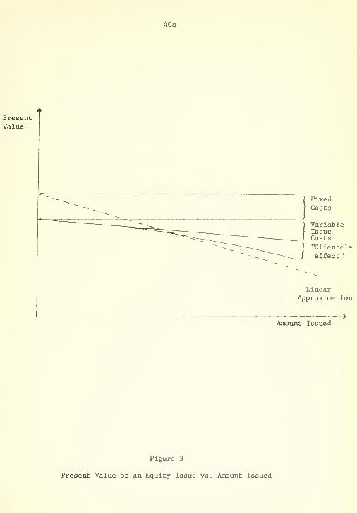
3. New issues of common stock deserve mention only because they tend

to he subject to increasing returns to scale.

The present value of an equity issue of any size would be

zero in a fully perfect market. However, the present value of

actual issues must reflect registration and underx<7riting fees

(largely fixed) and costs associated with the "clientele effect"

-- i.e., the necessity to give new shareholders a particularly

good "deal" to induce them to hold the firm's shares.

Figure 3 plots the probable present value of a stock issue

vs. the gross amount of the issue (solid curve). This curve is not

compatible with a linear objective function. Thus an approxi-

mation is necessary -- e.g., the dashed curve shown. This will

be an acceptable approximation if fairly large equity issues are

indicated by the LP solution, but misleading for small issues.

40a

FixedCosts

VariableIssueCosts

"Clienteleeffect"

LinearApproximation

Amount Issued

Figure 3

Present Value of an Equity Issue vs. Amount Issued

33

This difficulty is "built-in" and not amenable to easy solution.

4. Finally, in any practical context management will wish to add a

variety of further constraints dictated by the special circum-

stances in which the firm finds itself. Examples follow:

a. Some borrowing options may impose constraints on management.

E.g., restraints on working capital, dividend policy, and

new investments are frequently written into term loans.

b. There may be other scarce resources aside from capital,

and the program may be used to ration these among proposed

and existing projects. A common example is a shortage of

technical or managerial talent.

c. Other management goals may be reflected in constraints —

for example, management may vrish to insure that reported

income does not fall, or that the firm's overall employment

does not fluctuate too drastically.

CONCLUSION

L'he theory of fimmcial management presented in this paper can be

reasonably criticized on at least two grounds.

1. Simplified view of security valuation — The security valuation

models consistent with the LP approach are easier to believe

thiin prove, and also easier to disbelieve than disprove. But

there is no doubt that their derivation ignores some potentially

important considerations -- the observed capital market imperfec-

tions, and particularly the different tax rates on regular income

and capital gains. It cannot be proved that ignoring these factors

34

is a reasonable simplification.

2. The model yields a plan, not a strategy — The LP solution is a

schedule of financing and investment choices which are fully

appropriate in only one state of nature among the many that can

occur -- the state in which all cash flows turn out equal to

their expected values. Other possible outcomes affect the LP

plan chiefly through the "safety margins" built into the solution.

But the plan does not consider how the firm's future financial

dicisions may be dependent on future events. It does not pro-

vide the optimal financial strategy . Ideally, dynamic program-

ming should be used.

This is, of course, not an exhaustive list of faults.

Judged by the kind of model we would like to use, then, the LP

approach is not that exciting. Judged by the current theory of financial

management (essentially based on the cost of capital concept) the LP

approach is potentially a significant improvement.

35

APPENDIX A

DIFFICULTIES ASSOCIATED WITH THE

COST OF CAPITAL CONCEPT

The point of this appendix is that evaluating projects with the cost

of capital as usually measured is wholly reliable only when the projects are

19perpetuities. Strictly speaking, the point is not new, but it deserves

more emphasis than it has received.

Our analysis will be confined to the simple model of Section II above.

We assume the MM propositions hold so that Ft- = -i-!^ ^. From Eq . (6)^ (l+i)t ^ ' ^'

project j's Al'V, or net contribution to stock price, is

H(A.l) APVj = Aj + 5, [ZjtiTc/(l+i)t]

t=0

The derivation of the usual cost of capital measures (Eqs. (8) and

(9)) from Eq . (6) assumes (1) that project j is a perpetuity and (2) that

j's debt capacity, Z =j. , is constant over time. These assumptions imply

that

(A. 2) APVi = —fj- - li + Z^Tp^ p(j) ^ ^

As is apparent from their derivation, Eqs. (8) and (9) do not apply

when assumptions (1) and/or (2) are violated. For our purposes, a simple

example suffices. Consider a project requiring an investment Ij and re-

turning 'a^ at t = 1. From Eq. (A.l),

19Modigliani and Miller [11]^ p. 434_, fn. 3.

36

APV, ail/Ii d.iTci = _Ji

—

I - 1 + -J

Dropping subscripts, rearranging, and defining y as APV^/I^ .

^•^''

1-b^i +

f>+ (l+i)(l-fy)

We now define a "true" cost of capital, p , as the rate which gives the

correct APV when used to discount the projects cash flows:

Sdl- - 1 = APV

(A. 4)

l+APV

substituting in Eq. (A. 3),

(A. 5) p = p - (.^+n^^'^<^If (1+i) (l+APV)•

It is easy to verify that p is not the same as P :

•?

p= o' = p(l-dTc)

If true, this would imply, using Eq. (A. 5) that

p (1 + y + iy) = i,

which is impossible if p > i and y = APV/l > 0. Thus p' will not

37

20evaluate single-period investments correctly.

The interested reader will not find it difficult to find other cases

in which the usual cost of capital measures are inappropriate.

It is natural to ask whether P = n(l-.2i!J^). Unfortunately^ thiis true only if y = 1/p , or if ' ^

APV/I = -i-,

P

APV = —(I).

As reasoiuible values for i— are 3, 4 or larger, this is a decidedly specialcase. f

38

REFERENCES

1. Nevins D. Baxter. "Leverage, Risk of Ruin and the Cost of Capital,"Journal of Finance , XXII (September 1967), 395-404.

2. R. Byrne, A. Charnes, A. A. Cooper and K. Kortanek. "Chance ConstrainedCapital Budgeting," Journal of Financial and Quantitative Analysis . II(December 1967), 339-64.

3. A. Charnes and A. A. Cooper. "Chance Constrained Programming,"Management Science

,(October 1959), 73-79.

4. A. Charnes, W. W. Cooper and M. Miller. "Application of Linear Pro-gramming to Financial Budgeting and the Costing of Funds," Journal ofBusiness , XXXII (January 1959), 20-46.

5. David Durand. "The Cost of Capital in an Imperfect Market: A Replyto Modigliani and Miller," American Economic Review . XLIX (September1959), 646-55.

6. John Lintner. "Dividends, Earnings, Leverage, Stock Prices and theSupply of Capital to Corporations," Review of Economics and Statistics .

XLIV (August 1962), 243-69.

"Optimal Dividends and Corporate Growth Under Uncertainty,Quarterly Journal of Economics , LXXVII (February 1964), 49-95.

"Security Prices, Risk and Maximal Gains from Diversifi-cation," Journal of Finance . XX (December 1965), 587-616,

. "The Valuation of Risk Assets and the Selection ofRisky Investments," Review of Economics and Statistics , XLVII (February1965), 13-37.

10. M. Miller and Franco Modigliani. "Dividend Policy, Growth and theValuation of Shares," Journal of Business , XXXIV (October 1961), 411-33.

11. Franco Modigliani and M. H. Miller. "Corporate Income Taxes and theCost of Capital: A Correction," American Economic Review , LIII (June1963), 433-43.

12. . "The Cost of Capital, CorporationFinance and the Theory of Investment," American Economic Review ,

XLVIII (June 1958), 261-97.

13. Stewart C. Myers. "Procedures for Capital Budgeting Under Uncertainty,"Industrial Management Review , Vol 9 (Spring 1968).

39

14. SLcwarL C. Myers. "A Time-State-Prefcrence Model of Security Valun-Llon." Journal oH l''lnancial and Quantitative Aruilysis . Ill (M^irch

1^)68), 1-34.

15. A. A. Robichek and J. McDonald. "The Cost of Capital Concept: Po-tential Use and Misuse," Financial Executive . (June 1965).

16. A. A. Robichek and S. C. Myers. "Conceptual Problems in the Use ofRisk-Adjusted Discount Rates," Journal of Finance . XXI (December 1966),727-30.

17. . Optimal Financing Decisions . EnglewoodCliffs. N. J.: Prentice-Hall, Inc., 1965.

18. . "Problems in the Theory of OptimalCapital Structure," Journal of Financial and Quantitative Analysis , I

(June 1966), 1-35.

19. Ezra Solomon. "Measuring a Conpany's Cost of Capital," Journal ofBusiness ,

(October 1955)

.

20. William F. Sharpe. "Capital Asset Prices: A Theory of Market Equil-ibrium Under Conditions of Risk," Journal of Finance . XIX (September1964), 425-42.

21. . "A Simplified Model for Portfolio Analysis,"Management Science , Vol. 9 (January 1963), 277-93.

22. Donald L. Tuttle and Robert H. Litzenberger . "Leverage, Diversificationand Capital Market Effects on a Risk-Adjusted Capital Budgeting Frame-work," Journal of Finance , XXIII (June 1968), 427-44.

23. H. Martin Weingartner. "Capital Budgeting of Interrelated Projects,"Management Science. XII (March 1966)

.

24. . Mathematical Programming and the Analysis ofCapital Budgeting Problems . Englewood Cliffs, N.J.: Prentice-Hall,Inc., 1963.

Date DueJii

'L

- 5^2-6?'

3 TDflD DD3 fi74 35fl

3 TDflD D03 TDS 384

nil II mill III! nil Mini III! iiiiii II mil mil III II

3 TDflD D03 fl74 3TD

W?-6^

rWH-fe"?'

3^/f-^3'

3 VofiQ DQ3 ^^05 ^'^^

iiiniiii'i!'i!i!ii!iirii'i!iiiiiiiiiii

1>H(>-^"^

II3 'IDaD DD3 fl7M 317

iiniriiiKiiniiiiii'

i'A7'G^

3 TDfiD DD3 fl73 Tflfi

111---

3"'?0aD''003 M04 ^57

3W-fc'?

3 TDfiO D03 TD5 3E7