S1

Liquid structure of the choline chloride-urea deep eutectic solvent (reline)

from neutron diffraction and atomistic modelling

Oliver S. Hammond,† Daniel T. Bowron,§ Karen J. Edler†

† Centre for Sustainable Chemical Technologies, University of Bath, Claverton Down, Bath

BA2 7AY, UK

§ ISIS Neutron and Muon Source, Science and Technology Facilities Council, Rutherford

Appleton Laboratory, Harwell Oxford, Didcot OX11 0QX, UK

E-mail: K.Edler@bath.ac.uk

Electronic Supplementary Material (ESI) for Green Chemistry.This journal is © The Royal Society of Chemistry 2016

S2

A) Theory

Neutron diffraction experiments rely on the often wide difference in coherent neutron

scattering lengths between atomic isotopes (bcoherent), for example hydrogen (bhydrogen = -3.74

fm) and deuterium (bdeuterium = 6.67 fm). Each sample that is measured with different H/D

isotopic substitutions therefore yields a different set of structural information corresponding

with the same overall structure, assuming that the substitution does not affect it. For each

sample, the differential scattering cross-section is measured, which is then calibrated and

background-corrected before subtracting the multiple and inelastic scattering. The product

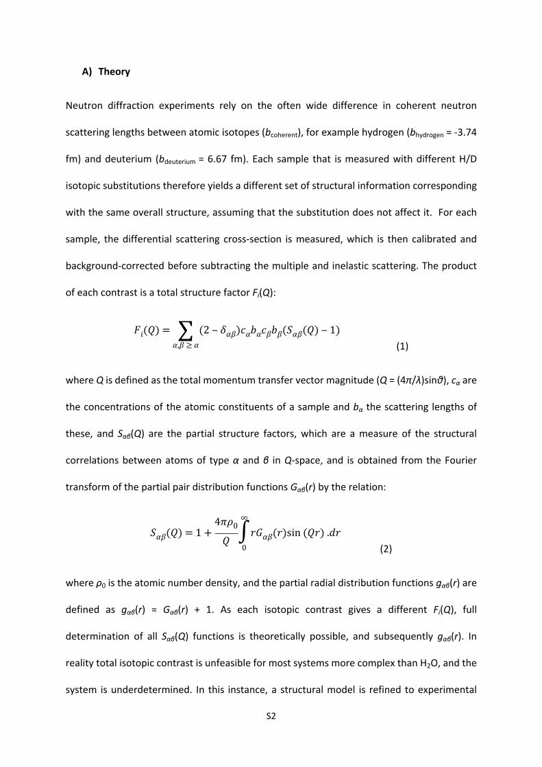
of each contrast is a total structure factor Fi(Q):

(1)𝐹𝑖(𝑄) = ∑

𝛼,𝛽 ≥ 𝛼

(2 ‒ 𝛿𝛼𝛽)𝑐𝛼𝑏𝛼𝑐𝛽𝑏𝛽(𝑆𝛼𝛽(𝑄) ‒ 1)

where Q is defined as the total momentum transfer vector magnitude (Q = (4π/λ)sinθ), cα are

the concentrations of the atomic constituents of a sample and bα the scattering lengths of

these, and Sαβ(Q) are the partial structure factors, which are a measure of the structural

correlations between atoms of type α and β in Q-space, and is obtained from the Fourier

transform of the partial pair distribution functions Gαβ(r) by the relation:

(2)𝑆𝛼𝛽(𝑄) = 1 +

4𝜋𝜌0

𝑄

∞

∫0

𝑟𝐺𝛼𝛽(𝑟)sin (𝑄𝑟) .𝑑𝑟

where ρ0 is the atomic number density, and the partial radial distribution functions gαβ(r) are

defined as gαβ(r) = Gαβ(r) + 1. As each isotopic contrast gives a different Fi(Q), full

determination of all Sαβ(Q) functions is theoretically possible, and subsequently gαβ(r). In

reality total isotopic contrast is unfeasible for most systems more complex than H2O, and the

system is underdetermined. In this instance, a structural model is refined to experimental

S3

data using the known physicochemical properties of the system as constraints such as density,

charge and molecular structure. This enables the extraction of the structural information of

the system with an atomistic level of detail.1

B) Empirical Potential Structure Refinement

Empirical potential structure refinement (EPSR) is a 3D structural modelling technique that

evolved from the reverse Monte Carlo (RMC) method.2,3 The purpose of EPSR is to simulate a

3D configuration that is the most objectively consistent with experimental diffraction data for

a system.4 To achieve a consistent fit to data, RMC uses hard sphere potentials and either

accepts or rejects a move depending on whether the fit has improved. Conversely, EPSR

employs a Lennard-Jones potential where εαβ and σαβ are given by typical Lorentz-Berthelot

mixing rules, using atom-centric point charges and periodic boundary conditions to generate

a simulated reference potential (RP) for a disordered system.5 The residuals between the RP

and the experimental data are used to calculate an empirical potential (EP) that is introduced

to the RP as a series of Poisson functions to suppress Fourier transform artefacts.6

EPSR uses a number of techniques to maximize the objectivity of the fit. Firstly, the properties

of a system, including its density, molecular structure, and composition, are used as severe

physicochemical constraints on configurations and their overlap. Secondly, EPSR deviates

from classical simulation by allowing a degree of intramolecular disorder that is obtained by

sampling harmonic potentials for each molecule, allowing for a better fit to experimental

data.7 To fit the diffraction data, the model is iteratively improved by adjusting the EP to bias

the model towards experimentally determined molecular configurations, with MC moves

accepted or rejected based around the Boltzmann factor:

S4

(3)𝑒𝑥𝑝[ ‒ {∆𝑈𝑖𝑛𝑡𝑟𝑎 +

1𝑘𝐵𝑇

(∆𝑈𝑅𝑃 + ∆𝑈𝐸𝑃)}]where ΔUintra,RP,EP are the energy differences between the new and old model configurations,

respectively due to the intramolecular, reference, and empirical potentials.

C) Simulation method

A set of molecules are first constructed to impose the mean intramolecular geometry by using

interatomic distance constraints, shown in the main text. These molecules are then

parameterized by assigning Lennard-Jones, charge, and atomic mass values to each distinct

atom type, which can be seen in Table 1. Parameters for urea were derived from those used

by Soper et al. in previous diffraction experiments on the aqueous structure of urea at very

high concentrations,8 and parameters for choline and chloride are derived from the OPLS All-

Atom force field potential.9 200 choline, 200 chloride and 400 urea molecules are introduced

to a simulation box which is randomized to generate a disordered starting configuration. The

density is initially set to 1/20 of the experimental value to minimize the probability of

molecular overlap.

The simulation is allowed to equilibrate in energy by running for a number of MC cycles,

where one cycle comprises an attempt to move every atom, rotate every rotational group,

and rotate and translate every molecule one time each. The box is compressed by

approximately 10% and the process repeated until the experimental density of 0.106 atoms

Å-3 is obtained. Using the reference potential only, the simulation continues to run until the

energy of the system reaches a plateau. By this point, the simulation has equilibrated as a

cubic box of diameter 41.6 Å, allowing reliable determination of structures up to d/2 = 20.8 Å

S5

in size. The empirical potential is then introduced to begin the refinement against the neutron

data, with one refinement cycle comprising five MC cycles and the recalculation of the EP.

Following equilibration of the model, the simulation is begun by accumulating statistics over

thousands of refinement cycles on the EP and all of the structural information within the

model, such as RDFs, SDFs, and coordination numbers. Molecular centre radial distribution

functions and spatial density functions that describe the configurations of cations, anions and

urea molecules around one another are determined using the spherical harmonics (SHARM)

routine of EPSR, and liquid ‘hole’ sites are determined using the VOIDS routine.

S6

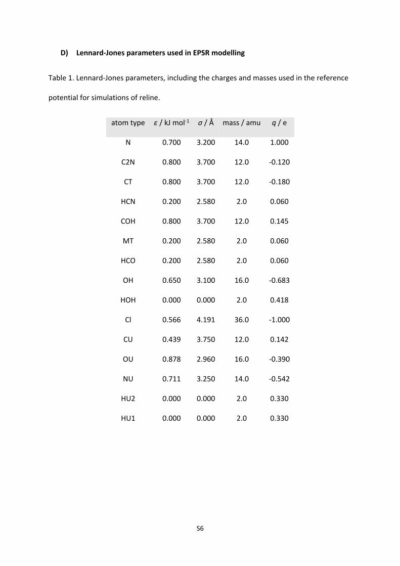
D) Lennard-Jones parameters used in EPSR modelling

Table 1. Lennard-Jones parameters, including the charges and masses used in the reference

potential for simulations of reline.

atom type ε / kJ mol-1 σ / Å mass / amu q / e

N 0.700 3.200 14.0 1.000

C2N 0.800 3.700 12.0 -0.120

CT 0.800 3.700 12.0 -0.180

HCN 0.200 2.580 2.0 0.060

COH 0.800 3.700 12.0 0.145

MT 0.200 2.580 2.0 0.060

HCO 0.200 2.580 2.0 0.060

OH 0.650 3.100 16.0 -0.683

HOH 0.000 0.000 2.0 0.418

Cl 0.566 4.191 36.0 -1.000

CU 0.439 3.750 12.0 0.142

OU 0.878 2.960 16.0 -0.390

NU 0.711 3.250 14.0 -0.542

HU2 0.000 0.000 2.0 0.330

HU1 0.000 0.000 2.0 0.330

S7

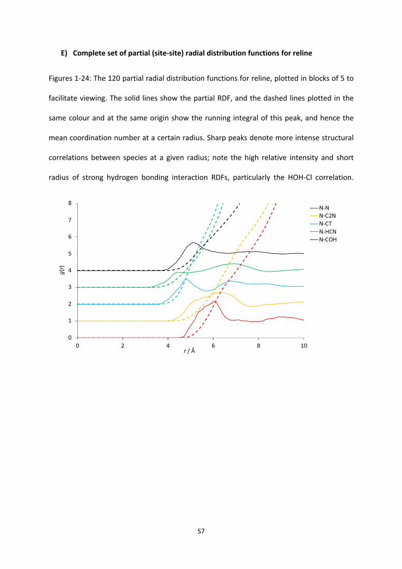
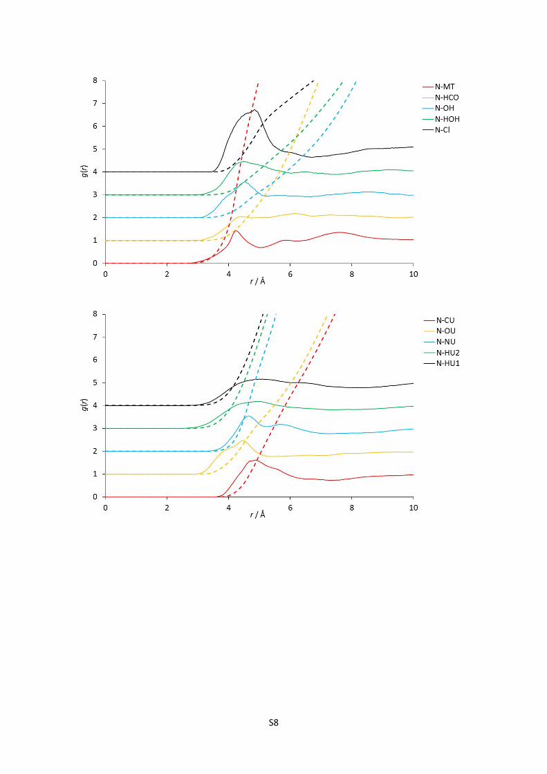
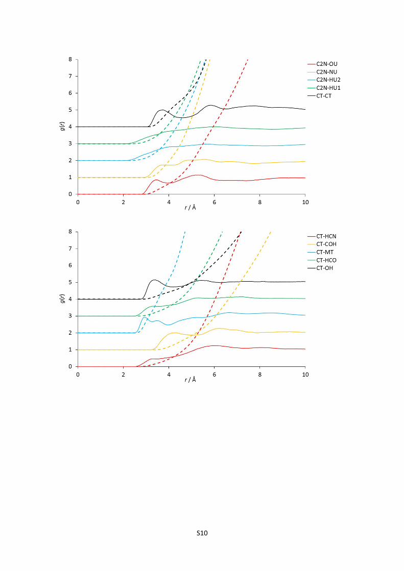
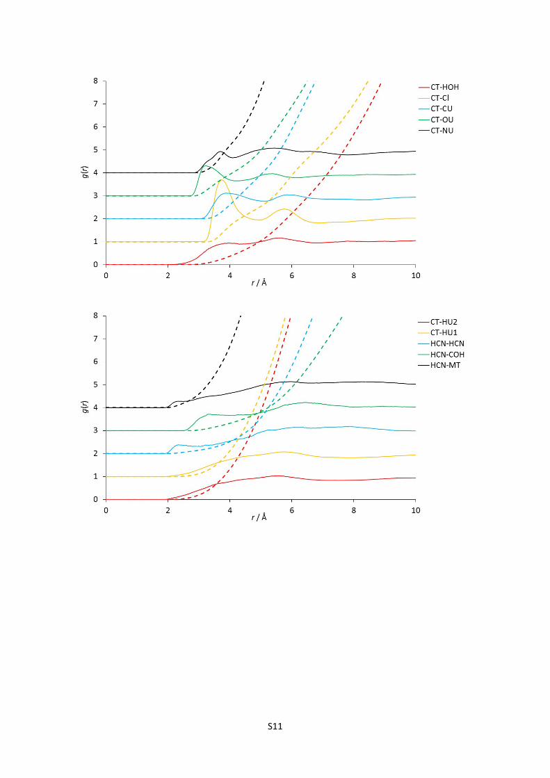
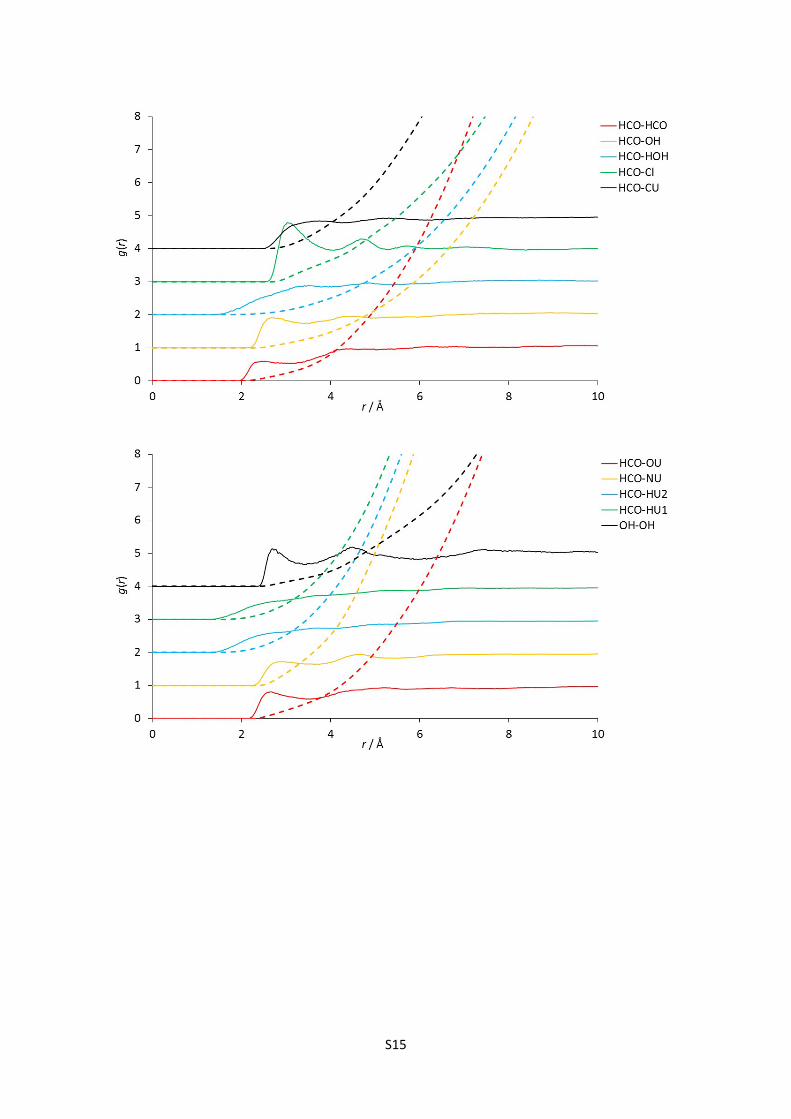
E) Complete set of partial (site-site) radial distribution functions for reline

Figures 1-24: The 120 partial radial distribution functions for reline, plotted in blocks of 5 to

facilitate viewing. The solid lines show the partial RDF, and the dashed lines plotted in the

same colour and at the same origin show the running integral of this peak, and hence the

mean coordination number at a certain radius. Sharp peaks denote more intense structural

correlations between species at a given radius; note the high relative intensity and short

radius of strong hydrogen bonding interaction RDFs, particularly the HOH-Cl correlation.

S8

S9

S10

S11

S12

S13

S14

S15

S16

S17

S18

S19

References

1 A. K. Soper, ISRN Phys. Chem., 2013, 2013, 279463.

2 A. C. Hannon, W. S. Howells and A. K. Soper, Inst. Phys. Conf. Ser., 1990, 107, 193–211.

3 R. L. McGreevy, J. Phys. Condens. Matter, 2001, 13, R877–R913.

4 A. K. Soper, Chem. Phys., 1996, 202, 295–306.

5 A. K. Soper, Chem. Phys., 2000, 258, 121–137.

6 A. K. Soper, Phys. Rev. B, 2005, 72, 104204.

7 A. K. Soper, Mol. Phys., 2001, 99, 1503–1516.

8 A. Soper, A. K., Castner, E. W., Luzar, Biophys. Chem., 2003, 105, 649–666.

9 W. L. Jorgensen, D. S. Maxwell and J. Tirado-Rives, J. Am. Chem. Soc., 1996, 118, 11225–

11236.