Service Engineering March 2013

LITTLE’S LAW

A conservation law that applies to the following general setting:

systeminput output

Input: Continuous flow or discrete units (examples: granules of powder measured in tons,tons of paper, number of customers, $1000’s).

System: Boundary is all that is required (very general, abstract).

Output: Same as input, call it throughput.

Two possible scenarios:• System during a “cycle” (empty → empty, finite horizon);

• System in steady state/in the long run (for example, over many cycles).

Quantities that are related via Little’s law:• λ = long-run average rate at which units arrive

(= long-run average rate at which units depart) = throughput-rate, whose units arequantity/time-unit or #/time-unit;

• L = long-run average inventory/quantity/number in the system(eg. WIP: Work-In-Process, customers);

• W = long-run average time a unit spends in the system = throughput time(eg. hours) = sojourn time.

Little’s Law L = λW

1

Motivation 1: λ customers/hour, each charged $1/hour while remaining in the system.Then λ×W is the rate at which the system generates cash which, in turn, “clearly” equalsL.

Motivation 2: If there is always a single customer (L = 1) in the system, and every cus-tomer remains in the system W hours on average (customers arrive one after the other),then λ = 1/W is clear. When there are L in the system, on the average, λ = L/W = L/Wis just one leap of faith.

Hint at a stochastic version: think of i.i.d sojourn times and use the Strong Law of LargeNumbers.

Motivation 3 (finite horizon): Consider a system that operates in a finite horizon (inter-val of time), and think of customers that arrive and leave (discrete units). Interval length isT .

Note: Littles Law will work if the system is empty at time 0, and empty at time T .

Motivation 4 (work in cycles): Consider a system that operates in cycles of equal dura-tions and has the same statistical behavior during each cycle. Cycle length is T .

Note: Littles Law will work if the system is at the same level (not necessarily 0) at thebeginning and at the end of the cycle, and if all the customers that are in the system at thebeginning of the cycle leave the system before the end of the cycle.This happens, for instance, if there is a moment during the cycle when the system becomesempty (see Example 10 on page 12, or Serfozos treatment on page 18).

Graphical representation. N customers flow though the system during a cycle.A customer is represented by a rectangle of unit height, whose length equals the time thecustomer spends in the system (see the figure below).

Motivation 5 (steady-state): Consider a system that is stable over long periods. Thelong-run average behavior will follow Little’s law.

2

!

"

#$%&'

()*+,-' .'/01#2%&31

4

56

!

"

#$%&'

7)#+'

4

!"#$%#& !"'$%#

*4

4 *

Note: Vertical cut = number of customers in the system.

S = Shaded area (units: customer ! hours), measures total waiting.

W =S

N, divides waiting among customers

(the customer’s view).

L =S

T, divides waiting over time

(the manager’s view).

! =N

T, implies L = ! · W

(which adds the server’s view).

8

Note: Vertical cut = number of customers in the system.

S = Shaded area (units: customer × hours), measures total waiting.

W =S

N, divides waiting among customers

(the customer’s view).

L =S

T, divides waiting over time

(the manager’s view).

λ =N

T, implies L = λ ·W

(which adds the server’s view).

3

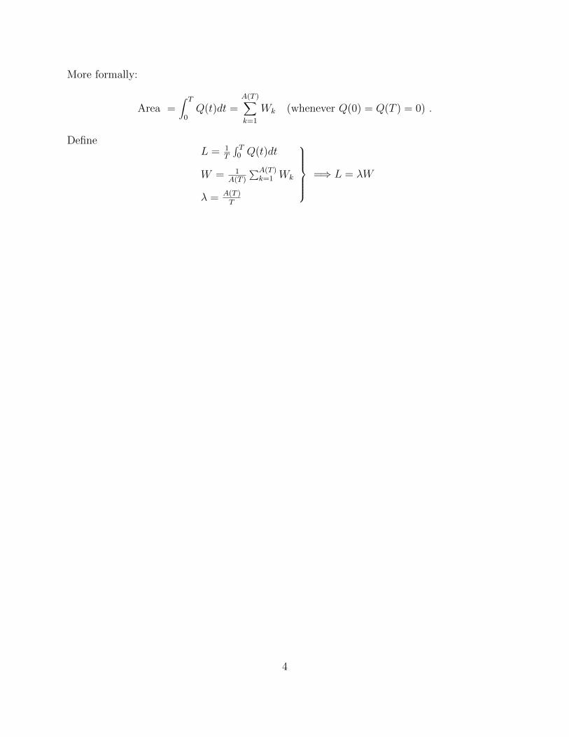
More formally:

Area =∫ T

0Q(t)dt =

A(T )∑k=1

Wk (whenever Q(0) = Q(T ) = 0) .

DefineL = 1

T

∫ T0 Q(t)dt

W = 1A(T )

∑A(T )k=1 Wk

λ = A(T )T

=⇒ L = λW

4

Empirical Examples

Little’s Law for Retail calls, May 2002: US Bank

!"#$%&'($)'*"+,*-."+-*,/0."1,2"34435"67"8,9:"!""#$%&'()*(*++,",-(.,)%#&(/*)%&

(0%12332

3

4333

53333

54333

23333

24333

63333

64333

73333

74333

43333

3 4 53 54 23 24 63

-%1'

89:;

,"(*

+(<%

','

""

;!"<=-%,(-";,/*/9("#/>-."+-*,/0."1,2"34435"67"8,9:"!"#$!$,"%=,(>%#)#?=(/#:,@(.,)%#&

0%1(2332A(BC(D%?E

3

4

53

54

23

24

63

64

73

3 4 53 54 23 24 63

-%1'

0,%?

'@(C

,<*?

-'

""

?!"<=-%,(-"@'-'-"?-9(*$."+-*,/0."1,2"34435"67"8,9:%!&#$"!"#$%&'()*%"+,"-$)$)"./0)*12)3"4)&1+5

617"8998:";<"=1,>

9

?

8

@

A

B

C

9 B ?9 ?B 89 8B @9

D17%

/0)*12)"E$(F)*"+,"-$)$)

!"#$%&'()*%"+,"-$)$) G+&&5)H%"G1I "

J1&) ? 8 @ A B C K L M ?9 ?? ?8 ?@ ?A ?B ?C

!"#$% !%&## !$#&# &#&'# $&($ !")"$ !!)$* !!**( !!!#' !#((' &#"($ $&#& #&*'! !$%)! !%"$* !)*%%N )+% !+! "+( &(+( %+& *+% &+' &+' &+" !+" &(+) #+" !+) !+# %+" #+*"O"N *+#' &+!' !+#" &+%) (+)( &+&# (+$# (+$# (+%' &+)( &+$' (+#( &+%' &+#$ *+'& &+$&G *+)( &+#( !+#' &+%% (+)( &+&) (+$# (+$# (+$& &+)& &+"& (+#( &+$& &+#$ *+'# &+$!

J1&) ?K ?L ?M 89 8? 88 8@ 8A 8B 8C 8K 8L 8M @9 @?

!)!!" &))!! $)!( #()!# !)#'! !#($( !#(() !*)&* &!&(( )'(' &))" #!'"( !"&%! !"#&% #(*"#N )+# *$+% "+& !+( *+& *+& !+* !+) *+! %+# !$+( %+) *+$ *+) !+*"O"N *+&' #+'% (+$& &+#& (+"$ (+"! &+*) &+!( (+!) (+## (+%$ !+*' &+&" &+&& &+#$G *+*( #+'$ (+$& &+#* (+"" (+"# &+*$ &+!& (+!$ (+## (+%$ !+!( &+*( &+&* &+#" "

25

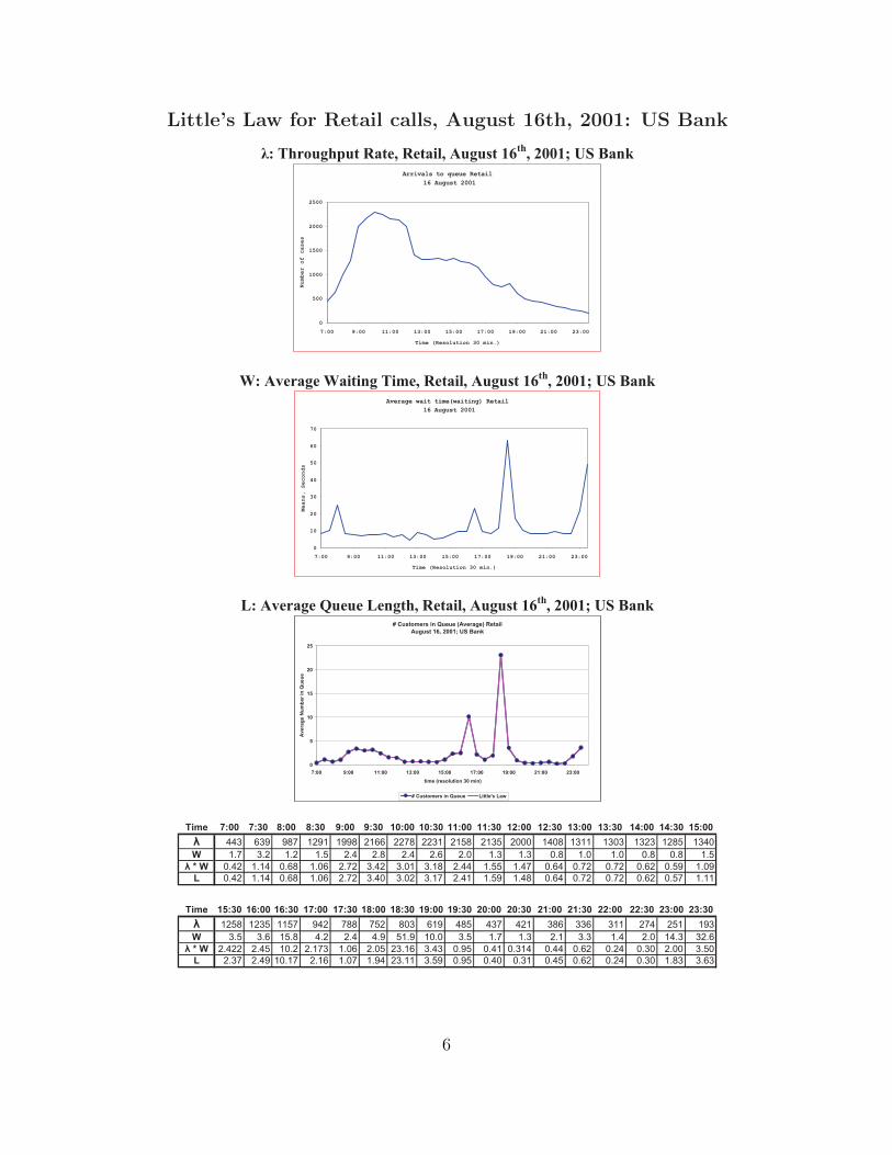
Little’s Law for Retail calls, August 16th, 2001: US Bank

!"#$%&'($)'*"+,*-."+-*,/0."1'('2*"34*$."56637"89":,;<"!""#$%&'()*(+,-,-(.-)%#&

(/0(!,1,')(233/

3

433

/333

/433

2333

2433

5633 7633 //633 /8633 /4633 /5633 /7633 2/633 28633

9#:-(;.-'*&,)#*<(83(:#<=>

?,:@

-"(*

A(B%

'-'

=!"1>-%,(-"=,/*/;("#/?-."+-*,/0."1'('2*"34*$."56637"89":,;<"!$-"%1-(C%#)()#:-;C%#)#<1>(.-)%#&

(/0(!,1,')(233/

3

/3

23

83

D3

43

03

53

5633 7633 //633 /8633 /4633 /5633 /7633 2/633 28633

9#:-(;.-'*&,)#*<(83(:#<=>

E-%<

'F(G

-B*<

H'

"

@!"1>-%,(-"A'-'-"@-;(*$."+-*,/0."1'('2*"34*$."56637"89":,;<"!"#$%&'()*%"+,"-$)$)"./0)*12)3"4)&1+5

/$2$%&"678"9::6;"<=">1,?

:

@

6:

6@

9:

9@

AB:: CB:: 66B:: 6DB:: 6@B:: 6AB:: 6CB:: 96B:: 9DB::

&+()".*)%'5$&+',"D:"(+,3

/0)*12)"E$(F)*"+,"-$)$)

!"#$%&'()*%"+,"-$)$) G+&&5)H%"G1I

J+() AB:: ABD: KB:: KBD: CB:: CBD: 6:B:: 6:BD: 66B:: 66BD: 69B:: 69BD: 6DB:: 6DBD: 6LB:: 6LBD: 6@B::

!!" #"$ $%& '($' '$$% ('## ((&% (("' (')% ('") (*** '!*% '"'' '"*" '"(" '(%) '"!*M '+& "+( '+( '+) (+! (+% (+! (+# (+* '+" '+" *+% '+* '+* *+% *+% '+)"N"M *+!( '+'! *+#% '+*# (+&( "+!( "+*' "+'% (+!! '+)) '+!& *+#! *+&( *+&( *+#( *+)$ '+*$G *+!( '+'! *+#% '+*# (+&( "+!* "+*( "+'& (+!' '+)$ '+!% *+#! *+&( *+&( *+#( *+)& '+''

J+() 6@BD: 67B:: 67BD: 6AB:: 6ABD: 6KB:: 6KBD: 6CB:: 6CBD: 9:B:: 9:BD: 96B:: 96BD: 99B:: 99BD: 9DB:: 9DBD:

'()% '(") '')& $!( &%% &)( %*" #'$ !%) !"& !(' "%# ""# "'' (&! ()' '$"M "+) "+# ')+% !+( (+! !+$ )'+$ '*+* "+) '+& '+" (+' "+" '+! (+* '!+" "(+#"N"M (+!(( (+!) '*+( (+'&" '+*# (+*) ("+'# "+!" *+$) *+!' *+"'! *+!! *+#( *+(! *+"* (+** "+)*G (+"& (+!$ '*+'& (+'# '+*& '+$! ("+'' "+)$ *+$) *+!* *+"' *+!) *+#( *+(! *+"* '+%" "+#"

36

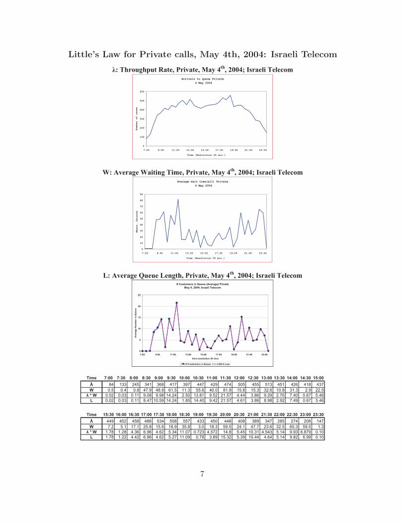
Little’s Law for Private calls, May 4th, 2004: Israeli Telecom

!"#$%&'($)'*"+,*-."/%01,*-."2,3"4*$."56647"89%,-:0"#-:-;&<!""#$%&'()*(+,-,-(."#$%)-

(/(0%1(233/

3

433

233

533

/33

633

733

8933 :933 44933 45933 46933 48933 4:933 24933 25933

;#<-(=>-'*&,)#*?(53(<#?@A

B,<C

-"(*

D(E%

'-'

=!">1-%,(-"=,0*0?("#0<-."/%01,*-."2,3"4*$."56647"89%,-:0"#-:-;&<"!$-"%F-(G%#)()#<-=%&&A(."#$%)-

(/(0%1(233/

3

43

23

53

/3

63

73

83

H3

:3

8933 :933 44933 45933 46933 48933 4:933 24933 25933

;#<-(=>-'*&,)#*?(53(<#?@A

0-%?

'I(J

-E*?

K'

""

@!">1-%,(-"A'-'-"@-?(*$."/%01,*-."2,3"4*$."56647"89%,-:0"#-:-;&<"!"#$%&'()*%"+,"-$)$)"./0)*12)3"4*+01&)

516"78"9::7;"<%*1)=+">)=)?'(

:

@

A:

A@

9:

9@

BC:: DC:: AAC:: AEC:: A@C:: ABC:: ADC:: 9AC:: 9EC::

&+()".*)%'=$&+',"E:"(+,3

/0)*12)"F$(G)*"+,"-$)$)

!"#$%&'()*%"+,"-$)$) H+&&=)I%"H1J

>+() BC:: BCE: KC:: KCE: DC:: DCE: A:C:: A:CE: AAC:: AACE: A9C:: A9CE: AEC:: AECE: A7C:: A7CE: A@C::!" #$$ %"& $"# $'! "#( $)( ""( "%) "(" &*& "&& &#$ "&# "%' "#! "$(

L *+& *+" *+! "(+) "!+! '#+& ##+$ &&+' "*+* !#+) #&+! #&+$ $%+' #*+! $#+$ %+) %%+&"M"L *+*% *+*$ *+## )+*! )+)! #"+%" %+&* #$+!# )+&% %#+&( "+"" $+!' )+%) %+(* (+"* *+'( &+"'H *+*% *+*$ *+## !+"( #*+&) #"+%" #+!& #"+"* )+"% %#+&( "+'# $+!' !+)! %+)% (+") *+'( &+"'

>+() A@CE: ANC:: ANCE: ABC:: ABCE: AKC:: AKCE: ADC:: ADCE: 9:C:: 9:CE: 9AC:: 9ACE: 99C:: 99CE: 9EC:: 9ECE:"") "&% "&! "!' &$" &*! &&( "$$ "&* ""! "*! $!) $"( %!& %(" %*! #"(

L (+% &+# #(+# %&+! #&+' #!+) $&+! $+* #!+$ &)+& %"+# "(+( %$+' $%+& '&+$ &)+& #+$"M"L #+(! #+%! "+$' '+)' "+'% &+$" ##+*( *+(%$ "+&(% #"+! &+"& #*+$# "+&"$ &+#" )+)$ '+!() *+#*H #+(! #+%% "+"% '+)' "+'% &+%( ##+*) *+(! $+!) #&+$% &+$) #*+"" "+'" &+#" )+!% '+)) *+#* "

47

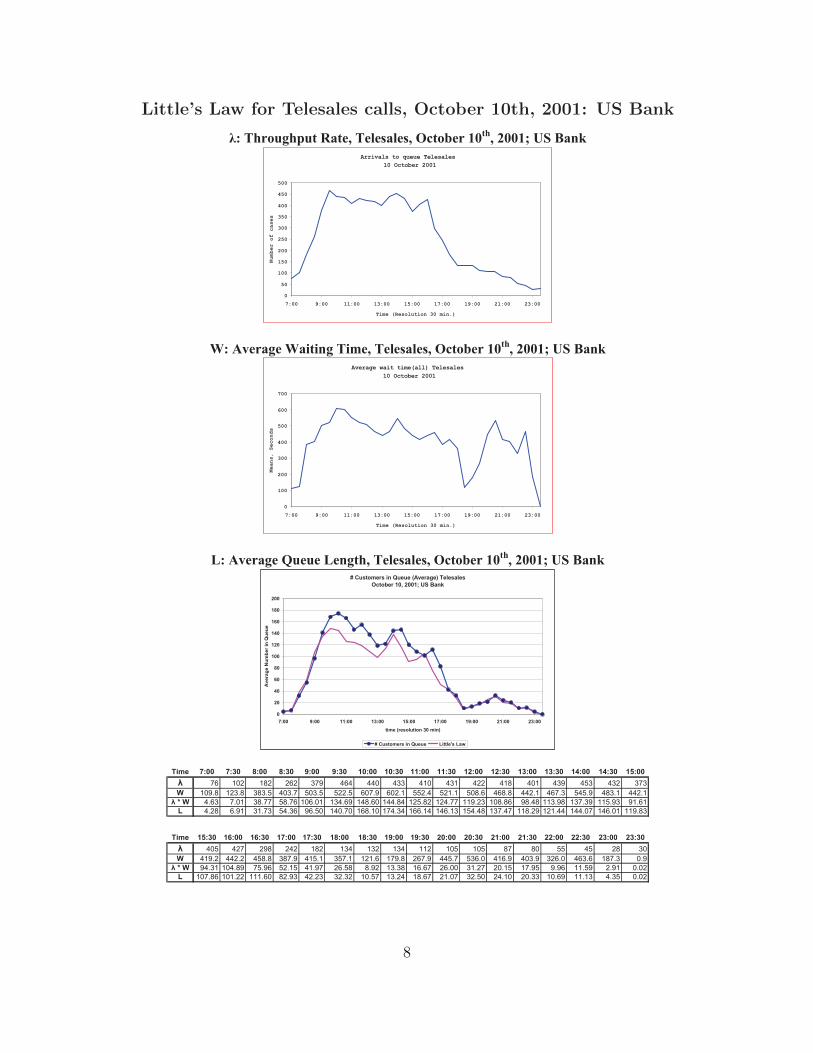
Little’s Law for Telesales calls, October 10th, 2001: US Bank

!"#$%&'($)'*"+,*-."#-/-0,/-0."12*&3-%"45*$."65547"89":,;<!""#$%&'()*(+,-,-(.-&-'%&-'

(/0(12)*3-"(400/

0

50

/00

/50

400

450

600

650

700

750

500

8900 :900 //900 /6900 /5900 /8900 /:900 4/900 46900

.#;-(<=-'*&,)#*>(60(;#>?@

A,;3-"(*B(2%'-'

"

=!">?-%,(-"=,@*@;("#@A-."#-/-0,/-0."12*&3-%"45*$."65547"89":,;<"!$-"%C-(D%#)()#;-<%&&@(.-&-'%&-'

(/0(12)*3-"(400/

0

/00

400

600

700

500

E00

800

8900 :900 //900 /6900 /5900 /8900 /:900 4/900 46900

.#;-(<=-'*&,)#*>(60(;#>?@

F-%>'G(H-2*>I'

"

B!">?-%,(-"C'-'-"B-;(*$."#-/-0,/-0."12*&3-%"45*$."65547"89":,;<"!"#$%&'()*%"+,"-$)$)"./0)*12)3"4)5)%15)%

67&'8)*"9:;"<::9=">?"@1,A

:

<:

B:

C:

D:

9::

9<:

9B:

9C:

9D:

<::

EF:: GF:: 99F:: 9HF:: 9IF:: 9EF:: 9GF:: <9F:: <HF::

&+()".*)%'5$&+',"H:"(+,3

/0)*12)"J$(8)*"+,"-$)$)

!"#$%&'()*%"+,"-$)$) K+&&5)L%"K1M

4+() EF:: EFH: DF:: DFH: GF:: GFH: 9:F:: 9:FH: 99F:: 99FH: 9<F:: 9<FH: 9HF:: 9HFH: 9BF:: 9BFH: 9IF::

!" #$% #&% %"% '!( )") ))$ )'' )#$ )'# )%% )#& )$# )'( )*' )'% '!'N #$(+& #%'+& '&'+* )$'+! *$'+* *%%+* "$!+( "$%+# **%+) *%#+# *$&+" )"&+& ))%+# )"!+' *)*+( )&'+# ))%+#"O"N )+"' !+$# '&+!! *&+!" #$"+$# #')+"( #)&+"$ #))+&) #%*+&% #%)+!! ##(+%' #$&+&" (&+)& ##'+(& #'!+'( ##*+(' (#+"#K )+%& "+(# '#+!' *)+'" ("+*$ #)$+!$ #"&+#$ #!)+') #""+#) #)"+#' #*)+)& #'!+)! ##&+%( #%#+)) #))+$! #)"+$# ##(+&'

4+() 9IFH: 9CF:: 9CFH: 9EF:: 9EFH: 9DF:: 9DFH: 9GF:: 9GFH: <:F:: <:FH: <9F:: <9FH: <<F:: <<FH: <HF:: <HFH:

)$* )%! %(& %)% #&% #') #'% #') ##% #$* #$* &! &$ ** )* %& '$N )#(+% ))%+% )*&+& '&!+( )#*+# '*!+# #%#+" #!(+& %"!+( ))*+! *'"+$ )#"+( )$'+( '%"+$ )"'+" #&!+' $+("O"N ()+'# #$)+&( !*+(" *%+#* )#+(! %"+*& &+(% #'+'& #"+"! %"+$$ '#+%! %$+#* #!+(* (+(" ##+*( %+(# $+$%K #$!+&" #$#+%% ###+"$ &%+(' )%+%' '%+'% #$+*! #'+%) #&+"! %#+$! '%+*$ %)+#$ %$+'' #$+"( ##+#' )+'* $+$%

"

5

8

Examples

1. Management Strategy and Control: Only two out of the three λ, L,W determinea strategy; the third is implicitly determined.

Scenario: λ = demand (projected), W = goal (set), L = means of monitoring W .

2. Inventory Management

L = average inventory;W = average time in inventory;λ = average throughput rate.

The quantity 1/W = λ/L is often referred to as the turnover ratio.

Scenario: A fast food restaurant processes on the average 5000 lbs. of hamburger perweek. The observed inventory level of raw meat, over a long period of time, averages2500 lbs.Data:L = 2500 lbs., λ = 5000 lbs./week;W = L/λ = 2500/5000 = 1/2 week is the average time spent by a pound of meat ininventory; 1/W = 2 times per week is the inventory turnover ratio.

3. Emergency Department (ED) Management

L = average number of patients;W = average time in hospitalization;λ = average arrival rate of patients per day;N = Number of beds = static capacity of the system.

The quantity f = λ/N is often referred to as the flux.The quantity ρ = L/N is often referred to as the occupancy. (N (the static capacity)must be at least L to calculate occupancy)

Scenario: An ED has 25 beds. It admits 240 patients per day. ED process takes onaverage 2 hours.Data:W = 2 hours, λ = 240 patients/day = 10 patients/hour;L = λW = 10 · 2 = 20 beds are occupied on average; 1/W = λ/L = 12 patients perday is the patients turnover ratio.f = λ/N = 240/25 ≈ 10 patients per bed.ρ = L/N = λW/N = fW = 20/25 = 0.8 = 80% beds occupancy.

9

4. Services Management

L = average number of customers;W = average customer’s delay;λ = average customers’ throughput rate.

Scenario:

(a) The restaurant in Example 3 processes on the average 1500 customers per day(=15 hours). On the average, there are 50 customers waiting to place an order,waiting for an order to arrive or eating.

λ = 1500 customers/day = 100 customers/hour;L = 50 customers;W = L/λ = 50/100 = 1/2 hours, average time in the restaurant.

(b) Out of the 50 customers, 40 customers on the average are eating.

λ = 100, L = 50− 40 = 10 customers at the service counter;W = L/λ = 10/100 hours = 6 minutes average wait at the counter.

5. Insurance: An insurance company processes 10,000 claims per year. The averageprocessing time of a claim is 3 weeks. Assuming 50 weeks per year, we have

λ = 10,000 claims/year = 200 claims/week;W = 3 weeks;L = λW = 3× 200 = 600 claims backlog on the average.

6. Loss Queues: Customers arrive at a service facility at rate α. A fraction β of them areblocked (do not enter). The others join a queue and wait until being served. Assumingexistence of averages and flow conservation, letτ = average service time,ν = long-run time-average number of customers in service. (Think G/G/S/N.)

Thenβ = 1− ν

ατ· (Any three of (α, β, τ, ν) determine the fourth.)

By: system = servers, L = ν, W = τ, λ = α(1− β).

Alternative scenario: An Internet site. (Think G/G/s/s.)S = number of servers. Then ρ = ν/S is servers’ utilization and

β = 1− ρS

ατ,

where (S, τ) are known, ρ is measured, hence α and β determine each other. One couldalso use this to determine an appropriate S, given service level.

10

Additional Examples

7. Process Flow: A supermarket receives from suppliers 300 tons of fish over the courseof a full year, which averages out to 25 tons per month. The average quantity of fishheld in freezer storage is 16.5 tons.On average, how long does a ton of fish remain in freezer storage between the time itis received and the time it is sent to the sales department?

W = L/λ = 16.5/25 = 0.66 months, on average, is the period that a ton of fish spendsin the freezer.How does one get L = 16.5? This comes out of the following inventory build-updiagram by calculating the area below the graph:

Inventory/Queue Build-up Diagram.

The data is from a bank call center. Each point corresponds to a 15-minute period ofa day (Sunday to Thursday), starting at 7:00am, ending at midnight, and averagedover the whole year of 1999.

• Why a positive y-intercept?

• What about experienced customers?

7. Loan Application Flow from Managing Business Process Flows, by R.Anupindi,S.Chopra, S.Deshmukh, J.Van Mieghem, E.Zemel, Chapter 3. (In Recitation.)

8. Process Flow: A supermarket receives from suppliers 300 tons of fish over thecourse of a full year, which averages out to 25 tons per month. The average quantityof fish held in freezer storage is 16.5 tons.On average, how long does a ton of fish remain in freezer storage between the timeit is received and the time it is sent to the sales department?

W = L/λ = 16.5/25 = 0.66 months, on average, is the period that a ton of fishspends in the freezer.How does one get L = 16.5? This comes out of the following inventory build-updiagram by calculating the area below the graph:

Inventory/Queue Build-up Diagram.

Thus, the company hires an average of 194.6 + 144 = 338.6 new employees permonth, or equivalently, 338.6 × 12 = 4063.2 new employees per year.

4063.2

36, 000= 0.1128 × 100% = 11.28% labor turnover during a year

= 2.82% turnover during a 3-month period

(compared with 40% at fast food, for example

and about 100% in many Call Centers).

10. Process Flow: A supermarket receives from suppliers 300 tons of fish over thecourse of a full year, which averages out to 25 tons per month. The average quantityof fish held in freezer storage is 16.5 tons.On average, how long does a ton of fish remain in freezer storage between the timeit is received and the time it is sent to the sales department?

W = L/λ = 16.5/25 = 0.66 months, on average, is the period that a ton of fishspends in the freezer.How does one get L = 16.5? This comes out of the following inventory build-updiagram by calculating the area below the graph:

Inventory/Queue Build-up Diagram.

0

2

4

6

8

10

12

14

16

18

20

22

24

26

28

30

0 1 2 3 4 5 6 7 8 9 10 11 12

time (months)

inve

ntor

y L(

t)

17 × 412

+ 24 × 412

+ 12 × 212

+ 5 × 212

= 16.5

7

17 × 412

+ 24 × 412

+ 12 × 212

+ 5 × 212

=

173

+ 8 + 2 + 56

= 16.5.

14

17× 412

+ 24× 412

+ 12× 212

+ 5× 212

=

173

+ 8 + 2 + 56

= 16.5.

8. Workforce ManagementA certain Japanese company has 36,000 employees, 20% of whom are women. Theaverage term of employment for a woman is 37 months, whereas for men it is 200months. Assume that the total employment level and the mix of men and women arestable over time.

11

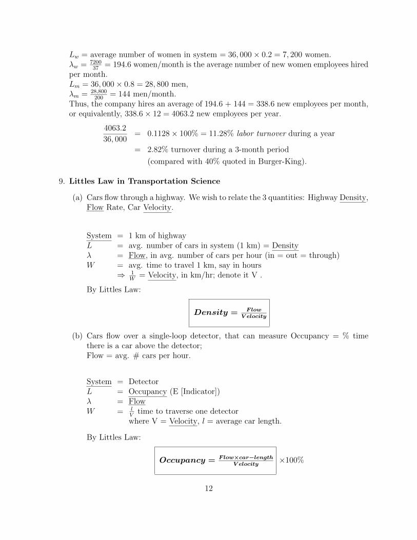
Lw = average number of women in system = 36, 000× 0.2 = 7, 200 women.λw = 7200

37= 194.6 women/month is the average number of new women employees hired

per month.Lm = 36, 000× 0.8 = 28, 800 men,λm = 28,800

200= 144 men/month.

Thus, the company hires an average of 194.6 + 144 = 338.6 new employees per month,or equivalently, 338.6× 12 = 4063.2 new employees per year.

4063.2

36, 000= 0.1128× 100% = 11.28% labor turnover during a year

= 2.82% turnover during a 3-month period

(compared with 40% quoted in Burger-King).

9. Littles Law in Transportation Science

(a) Cars flow through a highway. We wish to relate the 3 quantities: Highway Density,Flow Rate, Car Velocity.

System = 1 km of highwayL = avg. number of cars in system (1 km) = Densityλ = Flow, in avg. number of cars per hour (in = out = through)W = avg. time to travel 1 km, say in hours

⇒ 1W

= Velocity, in km/hr; denote it V .

By Littles Law:

Density = F lowV elocity

(b) Cars flow over a single-loop detector, that can measure Occupancy = % timethere is a car above the detector;Flow = avg. # cars per hour.

System = DetectorL = Occupancy (E [Indicator])λ = FlowW = l

Vtime to traverse one detector

where V = Velocity, l = average car length.

By Littles Law:

Occupancy = F low×car−lengthV elocity

×100%

12

Note: Occupancy = Density × car-length.

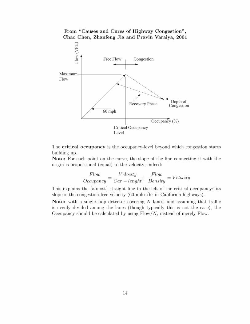
(c) Empirically, transportation flow reveals the following flow vs. occupancy relation(flow vs. density would look the same):

From “Causes and Cures of Highway Congestion”,Chao Chen, Zhanfeng Jia and Pravin Varaiya, 2001

5.2 Cars flow over a single-loop detector, that can measure Occupancy = % timethere is a car above the detector;Flow = avg. # cars per hour.

System = Detector

L = Occupancy (E [Indicator])

! = Flow

W = !V

time to traverse one detector

where V = Velocity, " = av. car length.

By Little’s Law:

Occupancy =Flow ! car-length

Velocity! 100%

Note: Occupancy = Density ! car-length.

5.3 Empirically, transportation flow reveals the following “flow vs. occupancy”relation (”flow vs. density” would look the same):

From “Causes and Cures of Highway Congestion”,Chao Chen, Zhanfeng Jia and Pravin Varaiya, 2001

!"##$%&%'(%)"*

+,-.)/)%0123

04##%012356((%7899.:.#;:<

=2;>#?@.2;5A;#99.:.#;@B"#4,@.2;

C#"@*%29=2;>#?@.2;

=4.@.:,1%B::/",;:<%D#E#1

FGH(%,)

'GIF%,)JG((%,)

K%

!"#$%& '( !)*+ ,-. *//$012/3 *2 1 -&/4"*2 14 0*-45")& 67.89 *2 :;8<=> 5"?2"#@4 4* 2**2*2 A/4*B&% 6> C<<<.

11

From “The freeway congestion paradox”,Chao Chen and Pravin Varaiya, 2001.

From “The freeway congestion paradox”,Chao Chen and Pravin Varaiya, 2001.!

!

"#$%

$&#%%

$$#!!

'#%%

"#%%

(#)%

(#&(

(#$%*#%%!

!"#$%&'(')*+#&,-"*+'.&#"+,'/-'0123'/45''67'8133'/49'.*-:',;&&<'/+<'=>*?':/@&'<%*;;&<'<%/4/-"A/>>75'

!!!!!!!!!!!!!!!!!!!!!!!!

From “Causes and Cures of Highway Congestion”,Chao Chen, Zhanfeng Jia and Pravin Varaiya, 2001

!""#$%&"'()*+

,-./()012+

3%456#6,-./

7.&89:;5.&,<99(,-./

=>(6$?

@9$;?(.A7.&89:;5.&B9".C9<'(1?%:9

7<5;5"%-(!""#$%&"'D9C9-

!"#$%& '( )*+&, *- .*/#&01"*/2 3- *..$45/.6 "0 75"/15"/&+ 8&,*9 .%"1".5, ,&:&,; 0&.1"*/

12

13

From “Causes and Cures of Highway Congestion”,Chao Chen, Zhanfeng Jia and Pravin Varaiya, 2001

From “The freeway congestion paradox”,Chao Chen and Pravin Varaiya, 2001.!

!

"#$%

$&#%%

$$#!!

'#%%

"#%%

(#)%

(#&(

(#$%*#%%!

!"#$%&'(')*+#&,-"*+'.&#"+,'/-'0123'/45''67'8133'/49'.*-:',;&&<'/+<'=>*?':/@&'<%*;;&<'<%/4/-"A/>>75'

!!!!!!!!!!!!!!!!!!!!!!!!

From “Causes and Cures of Highway Congestion”,Chao Chen, Zhanfeng Jia and Pravin Varaiya, 2001

!""#$%&"'()*+

,-./()012+

3%456#6,-./

7.&89:;5.&,<99(,-./

=>(6$?

@9$;?(.A7.&89:;5.&B9".C9<'(1?%:9

7<5;5"%-(!""#$%&"'D9C9-

!"#$%& '( )*+&, *- .*/#&01"*/2 3- *..$45/.6 "0 75"/15"/&+ 8&,*9 .%"1".5, ,&:&,; 0&.1"*/

12

The critical occupancy is the occupancy-level beyond which congestion startsbuilding up.Note: For each point on the curve, the slope of the line connecting it with theorigin is proportional (equal) to the velocity; indeed:

Flow

Occupancy=

V elocity

Car − lenght ;Flow

Density= V elocity

This explains the (almost) straight line to the left of the critical occupancy: itsslope is the congestion-free velocity (60 miles/hr in California highways).

Note: with a single-loop detector covering N lanes, and assuming that trafficis evenly divided among the lanes (though typically this is not the case), theOccupancy should be calculated by using Flow/N , instead of merely Flow.

14

10. Abandonment: Calls arrive at a call center at rate α. A fraction Pab of them abandonsdue to impatience. Individual abandonment rate is θ.

Let Lq, Wq denote, respectively, the average number of customers waiting to be served,and the average queueing time (waiting for service). Then

α · Pab = θ · Lq.

But Lq = αWq, hencePab = θ ·Wq.

Thus, the abandonment rate is proportional to the average waiting time. This has beenconfirmed empirically for new (potential) customers. Indeed, (Pab,Wq) were observedand scatterplotted. The slope (via regression) can be used to estimate customers’(average) patience. The data is from a bank call center. Each point corresponds to

a 15-minute period of a day (Sunday to Thursday), starting at 7:00am, ending atmidnight, and averaged over the whole year of 1999.

• Why a positive y-intercept?

• What about experienced customers?

15

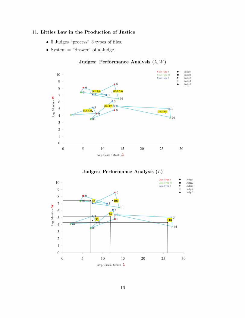
11. Littles Law in the Production of Justice

• 5 Judges “process” 3 types of files.

• System = “drawer” of a Judge.

Judges: Performance Analysis (λ,W )

15. Little’s Law in the “Production of Justice”.

• 5 Judges “process” 3 types of files.

• System = “drawer” of a Judge.

Judges: Performance Analysis (!, W )

!

""#

!

""#

"#

"

!

"#

!

""

!

"#

"

#

$

!

%

&

'

(

)

*

#"

" & #" #& $" $& !"

!"#$%&'#()& !*+#,%&'#()&

!$"#+%&(#,)

!*$%&(#-)&

!'#$%&(#")&

#

#

#

##

./01234&5267869:;<2&=;:>?3@3

+,-./012./"/ 3456.#+,-./012./"#/ 3456.$+,-./012./!/ 3456.!

3456.%3456.&

7869/:;<=>-/?/A

7869/+,-.-/@/:;<=>/?/

Judges: Performance Analysis (L)

!"#$%&'#()& !*+#,%&'#()&

!$"#+%&(#,)

!*$%&(#-)&

!'#$%&(#")&!

""#

!

""#

"#

"

!

"#

!

""

!

"#

"

#

$

!

%

&

'

(

)

*

#"

" & #" #& $" $& !"

#

#

#

##

(, *BB

&&& **C

,-

++

+,-./012./"/ 3456.#+,-./012./"#/ 3456.$+,-./012./!/ 3456.!

3456.%3456.&

7869/:;<=>-/?/A

7869/+,-.-/@/:;<=>/?/

17

Judges: Performance Analysis (L)

15. Little’s Law in the “Production of Justice”.

• 5 Judges “process” 3 types of files.

• System = “drawer” of a Judge.

Judges: Performance Analysis (!, W )

!

""#

!

""#

"#

"

!

"#

!

""

!

"#

"

#

$

!

%

&

'

(

)

*

#"

" & #" #& $" $& !"

!"#$%&'#()& !*+#,%&'#()&

!$"#+%&(#,)

!*$%&(#-)&

!'#$%&(#")&

#

#

#

##

./01234&5267869:;<2&=;:>?3@3

+,-./012./"/ 3456.#+,-./012./"#/ 3456.$+,-./012./!/ 3456.!

3456.%3456.&

7869/:;<=>-/?/A

7869/+,-.-/@/:;<=>/?/

Judges: Performance Analysis (L)

!"#$%&'#()& !*+#,%&'#()&

!$"#+%&(#,)

!*$%&(#-)&

!'#$%&(#")&!

""#

!

""#

"#

"

!

"#

!

""

!

"#

"

#

$

!

%

&

'

(

)

*

#"

" & #" #& $" $& !"

#

#

#

##

(, *BB

&&& **C

,-

++

+,-./012./"/ 3456.#+,-./012./"#/ 3456.$+,-./012./!/ 3456.!

3456.%3456.&

7869/:;<=>-/?/A

7869/+,-.-/@/:;<=>/?/

1716

12. Loan Application Flow from Managing Business Process Flows, by R.Anupindi,S.Chopra, S.Deshmukh, J.Van Mieghem, E.Zemel, Chapter 3. (In Recitation.)

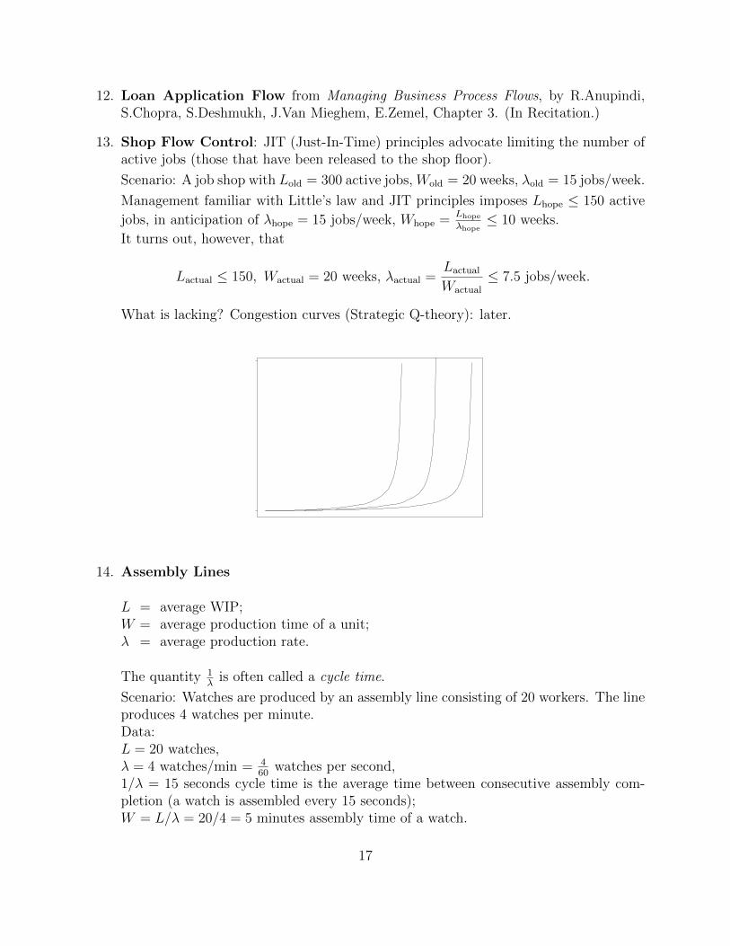
13. Shop Flow Control: JIT (Just-In-Time) principles advocate limiting the number ofactive jobs (those that have been released to the shop floor).

Scenario: A job shop with Lold = 300 active jobs, Wold = 20 weeks, λold = 15 jobs/week.

Management familiar with Little’s law and JIT principles imposes Lhope ≤ 150 active

jobs, in anticipation of λhope = 15 jobs/week, Whope =Lhope

λhope≤ 10 weeks.

It turns out, however, that

Lactual ≤ 150, Wactual = 20 weeks, λactual =Lactual

Wactual

≤ 7.5 jobs/week.

What is lacking? Congestion curves (Strategic Q-theory): later.

14. Assembly Lines

L = average WIP;W = average production time of a unit;λ = average production rate.

The quantity 1λ

is often called a cycle time.

Scenario: Watches are produced by an assembly line consisting of 20 workers. The lineproduces 4 watches per minute.Data:L = 20 watches,λ = 4 watches/min = 4

60watches per second,

1/λ = 15 seconds cycle time is the average time between consecutive assembly com-pletion (a watch is assembled every 15 seconds);W = L/λ = 20/4 = 5 minutes assembly time of a watch.

17

15. Cash Flow (Accounts Receivable): A company sells 300M$ worth of finished goodsper year. The average amount of accounts receivable is 45M$.

λ = 300M$/year;L = 45M$;W = L/λ = 45/300 = 0.15 years = 1.8 months.

So it takes, on average, 1.8 months from the time a customer is billed until the timepayment is received.

16. Cash Flow: A paper mill processes 40M$ of raw material per year. Direct conversioncosts are 20M$ per year. Average inventory cost (raw material + conversion) is 5M$.

λ = 40+20 = 60M$ year;L = 5M$;W = 5/60 = 1/12 years = 1 month.

Thus, there is an average lag of one month between the time a dollar enters the systemin the form of raw material (example: logs) or conversion cost (example: chemicals),and the time it leaves the system in the form of finished goods (example: paper).

18

Little’s Formula. Deterministic Model.Infinite Horizon (Stidham’s formulation)

departuresarrivals ratesystemrate

Averages: L = λ ·W

L = number of units in the system;λ = throughput rate;W = sojourn time.

Rigorous formulation

The system is characterized by {(An, Dn), n ≥ 1}, where

An – time of the nth arrival.Dn – departure-time of the nth arrival.

0 ≤ An ≤ An+1 An ≤ Dn <∞ .Define:A(t) = number of arrivals until t;D(t) = number of departures until t;L(t) = number of units such that An ≤ t < Dn, i.e., number of units in the system;Wn = Dn − An, sojourn time of the nth unit in the system.

Theorem. Assume that

λ = limt↑∞

1

tA(t) = lim

t↑∞

1

tD(t), 0 < λ <∞ .

Then

limN↑∞

1

N

N∑n=1

Wn = W exists ⇔ limT↑∞

1

T

∫ T

0L(t)dt = L exists ,

in which case L = λW .

19