Embed Size (px)
Citation preview
OPERATIONS RESEARCHVol. 61, No. 4, July–August 2013, pp. 1030–1045ISSN 0030-364X (print) � ISSN 1526-5463 (online) http://dx.doi.org/10.1287/opre.2013.1193
© 2013 INFORMS
Statistical Analysis with Little’s Law
Song-Hee Kim, Ward WhittDepartment of Industrial Engineering and Operations Research, Columbia University, New York, New York 10027
{[email protected], [email protected]}
The theory supporting Little’s Law (L = �W ) is now well developed, applying to both limits of averages and expectedvalues of stationary distributions, but applications of Little’s Law with actual system data involve measurements over afinite-time interval, which are neither of these. We advocate taking a statistical approach with such measurements. Weinvestigate how estimates of L and � can be used to estimate W when the waiting times are not observed. We advocateestimating confidence intervals. Given a single sample-path segment, we suggest estimating confidence intervals using themethod of batch means, as is often done in stochastic simulation output analysis. We show how to estimate and removebias due to interval edge effects when the system does not begin and end empty. We illustrate the methods with data froma call center and simulation experiments.
Subject classifications : Little’s Law; L= �W ; measurements; parameter estimation; confidence intervals; bias; finite-timeversions of Little’s Law; confidence intervals with L= �W ; edge effects in L= �W ; performance analysis.
Area of review : Stochastic Models.History : Received March 2012; revisions received August 2012, December 2012; accepted May 2013. Published online
in Articles in Advance August 7, 2013.
1. IntroductionWe have just celebrated the 50th anniversary of the famouspaper by Little (1961) on the fundamental queueing rela-tion L= �W with a retrospective by Little (2011) himself,which emphasizes the applied relevance as well as review-ing the advances in theory, including the sample-path proofby Stidham (1974) and the extension to H = �G. Severalbooks provide thorough treatments of the theory, includingthe sample-path analysis by El-Taha and Stidham (1999)and the stationary framework involving the Palm trans-formation by Sigman (1995) and Baccelli and Bremaud(2003), as well as the perspective within stochastic net-works by Serfozo (1999). As a consequence, L= �W andthe related conservation laws are now on a solid mathemat-ical foundation.
The relation L= �W can be quickly stated: The averagenumber of customers waiting in line (or items in a system),L, is equal to the arrival rate (or throughput) � multipliedby the average waiting time (time spent in system) per cus-tomer, W . If we know any two of these quantities, then wenecessarily know all three. The easily understood reason isreviewed in §2. With queueing models where � is known,the relation L= �W yields the value of L or W wheneverthe other has been calculated.
1.1. Measurements Over a Finite Time Interval
However, in many applications, these conservation lawsare applied with measurements over a finite-time intervalof length t, yielding finite averages L4t5, �4t51 and SW4t5(defined in (1) below). Indeed, the applied relevance withmeasurements motivated Little (2011) to discuss relations
among finite-time measurements instead of the stationaryframework in Little (1961). However, with finite averages,the large body of supporting theory often does not applydirectly, because that theory concerns either long-run aver-ages (limits) or the expected values of stationary stochasticprocesses in stochastic models. The available measurementsare neither of these.
Here is the essence of a typical application: We startwith the observation of L4s5, the number of items in thesystem at time s, for 0 ¶ s ¶ t. From that sample path,we can directly observe the arrivals (jumps up) and depar-tures (jumps down). Hence, we can easily estimate thearrival rate � and the average number in system L. How-ever, based only on the available information, we typicallycannot determine the time each item spends in the sys-tem, because the items need not depart in the same orderthat they arrived. Nevertheless, we can estimate the averagewaiting time by W = L/�, using our estimates of L and �.
In this paper we focus on the typical application in thepreceding paragraph, estimating W given estimates of Land �, illustrated by data from a large call center. The firstissue is that, with commonly accepted definitions (see (1)below), the relation L = �W is not valid as an equal-ity over a finite-time interval unless the system starts andends empty, which often is either not feasible or not desir-able. In §2 we review the exact relation that holds forfinite-time intervals and a way to modify the definitions sothat the edge effects do not occur, even when the systemdoes not start and end empty. Using modified definitionsto make L4t5 = �4t5SW4t5 valid for all finite intervals isthe approach of the “operational analysis” proposed by
1030
Kim and Whitt: Little’s LawOperations Research 61(4), pp. 1030–1045, © 2013 INFORMS 1031
Buzen (1976) and Denning and Buzen (1978), motivatedby performance analysis of computer systems, which isalso discussed by Little (2011). Changing definitions inthat way can be very helpful to check the consistency ofmeasurements and data analysis, which is a legitimate con-cern. Although changing the definitions is one option, weadvocate not doing so, because it leads to problems withinterpretation.
1.2. A Statistical Approach
We advocate taking a statistical approach with data over afinite-time interval. Thus we regard the finite averages asrealizations of random estimators of underlying unknown“true” values. We suggest estimating confidence intervals.Because the initial estimators may be biased, we suggestrefined estimators to reduce the bias. To the best of ourknowledge, a statistical approach has not been taken pre-viously in the literature on applications of L = �W withmeasurements; e.g., see Denning and Buzen (1978), Littleand Graves (2008), Little (2011), Lovejoy and Desmond(2011) and Mandelbaum (2011).
1.2.1. A Stationary Framework. Two very differentsettings can arise: stationary and nonstationary. Preliminarydata analysis should be done to determine if the data arefrom a stationary environment. In a stationary framework,we assume that Little’s Law theory applies, so that L, �1and W are well defined, corresponding to both means ofstationary probability distributions and limits of averages(assumed to exist), and related by L= �W . We thus regardthe underlying parameters L, �1 and W as the true valuesthat we want to estimate; we regard the averages L4t5, �4t51and SW4t5 based on measurements over a time interval [01 t]as estimates of these parameters.
To learn how well we know L, �1 and W when wecompute the averages L4t5, �4t51 and SW4t5, we suggestestimating confidence intervals. Given a single sample pathfrom an interval that can be regarded as approximately sta-tionary, we suggest applying the method of batch means toestimate confidence intervals, as is commonly done in sim-ulation output analysis, and has been studied extensively;e.g., see Alexopoulos and Goldsman (2004), Asmussen andGlynn (2007), Tafazzoli et al. (2011), Tafazzoli and Wilson(2011) and references therein. We present theory support-ing its application in the present context.
In addition, we are concerned with the statistical problemof how to make inferences from limited data. We illustrateby focusing on estimating W given the finite averages L4t5and �4t5 when the waiting times are not directly observed.We pay special attention to the indirect estimator SWL1�4t5≡
L4t5/�4t5 suggested by Little’s Law. We show the spe-cial definition used to obtain equality for L4t5= �4t5SW4t5within each subinterval seriously distorts the batch-meansestimators when the modified definition is used within eachsubinterval.
1.2.2. A Nonstationary Framework. However, manyapplications with data involve nonstationary settings; e.g.,service systems typically have arrival rates that vary sig-nificantly over each day. Estimation is more complicatedwithout stationarity, because conventional Little’s Law the-ory no longer applies. Indeed, the parameters L, �1 and W
are typically no longer well defined. To specify what weare trying to estimate, we assume that there is an unspec-ified underlying stochastic queueing model, which may behighly nonstationary (for which the processes in §2.1 arewell defined). As usual with Little’s Law, it is not necessaryto define the underlying queueing model in detail. Thenwe regard the vector of time averages 4L4t51 �4t51 SW4t55 asa random vector with an associated vector of finite meanvalues (E6L4t571E6�4t571E6SW4t57). We propose that meanvector as the quantity to be estimated.
Since the method of batch means is no longer appropriatewithout stationarity, we suggest an approach correspondingto independent replications. That approach is appropriatefor call centers when the data comes from multiple daysthat can be regarded as independent and identically dis-tributed. In a nonstationary setting, the bias can be muchmore important, so we discuss ways to reduce it.
1.2.3. Validation by Simulation. Because actual sys-tem data may be complicated and limited, we suggestapplying simulation to study how the estimation proceduresproposed here work for an idealized queueing model ofthe system. In doing so, we presume that we do not knowenough about the actual system to construct a model thatwe can directly apply to compute what we are trying toestimate, but that we know enough to be able to constructan idealized model to evaluate how the proposed estimationprocedures perform. We illustrate this suggested simulationapproach with our call center example in §3.2.
1.3. Organization
Here is how the rest of this paper is organized: In §2 wediscuss the finite-time version of L= �W , emphasizing theinterval edge effects. In §3 we apply the statistical approachto a banking call center example and associated simulationmodels. In §4 we study ways to estimate confidence inter-vals. In §5 we study ways to estimate and reduce the biasin the estimator SWL1�4t5 ≡ L4t5/�4t5. In §6 we performexperiments combining the insights in §§4 and 5; we esti-mate confidence intervals for refined estimators designedto reduce bias. Finally, in §7 we draw conclusions. Addi-tional material appears in the e-companion and a technicalreport (Kim and Whitt 2012) is available on the authors’web pages; the contents of both are described at the begin-ning of the e-companion. Kim and Whitt (2013) is a sequelto this paper on estimating waiting times with the time-varying Little’s Law. Supplemental material to this paper isavailable at http://dx.doi.org/10.1287/opre.2013.1193.
Kim and Whitt: Little’s Law1032 Operations Research 61(4), pp. 1030–1045, © 2013 INFORMS
2. Measurement Over a Finite TimeInterval: Definitions and Relations
In this section we review analogs of L = �W for a finite-time interval, denoted by [01 t]. Consistent with most appli-cations, we assume that the system was in operation in thepast, prior to time 0, and that it will remain in operationafter time t. We will use standard queueing terminology,referring to the items being counted as customers. We focuson the customers that are in the system at some time duringthe interval [01 t]. Let these customers be indexed in orderof their arrival time, which could be prior to time 0 if thesystem is not initially empty (with some arbitrary methodto break ties, if any).
2.1. The Performance Functions andTheir Averages
For customer k, let Ak be the arrival time, Dk the departuretime, and Wk ≡Dk −Ak the waiting time (time in system),where −� < Ak < Dk < �, 601 t7 ∩ 6Ak1Dk7 6= �1 and≡ denotes “equality by definition.” Let R405 count the cus-tomers that arrived before time 0 that remain in the systemat time 0; let A4t5 count the total number of new arrivals inthe interval [01 t]; and let L4t5 be the number of customersin the system at time t. Thus, A4t5= max 8k¾ 02 Ak ¶ t9−R405, t ¾ 0, and L405 = R405 + A405, where A405 is thenumber of new arrivals at time 0, if any. We will carefullydistinguish between R405 and L405, but the common caseis to have A405= 0 and L405=R405.
The respective averages over the time interval [01 t] are
�4t5≡ t−1A4t51 L4t5≡ t−1∫ t
0L4s5ds1
SW4t5≡ 41/A4t55R405+A4t5∑
k=R405+1
Wk1
(1)
where 0/0 ≡ 0 for SW4t5. The first two are time averages,whereas the last, SW4t5, is a customer average, but over allarrivals during the interval [01 t].
We will focus on these averages over [01 t] in (1), but wecould equally well consider the averages associated withthe first n arrivals. To do so, let Tn be the arrival epoch ofthe nth new arrival, i.e., Tn ≡An+R405, n¾ 0,
�n ≡ n/Tn1 Ln ≡ 41/Tn5∫ Tn
0L4s5ds1
SWn ≡ n−1R405+n∑
k=R405+1
Wk0
(2)
As in (1), the first two averages in (2) are time averages,but over the time interval [01 Tn], whereas the last, SWn, is acustomer average over the first n (new) arrivals. If there isonly a single arrival at time Tn, then the averages in (2) canbe expressed directly in terms of the averages in (1): �n =
�4Tn5, Ln = L4Tn51 and SWn = SW4Tn5, so that conclusionsfor (1) yield analogs for (2).
Just as we can use the relation L= �W and knowledge ofany two of the three quantities L, �1 and W to compute theremaining one, so we can use any two of the three estima-tors in (1) to create a new alternative estimator, exploitingL= �W :
LW1�4t5≡ �4t5SW4t51 �L1W 4t5≡L4t5
SW4t51 and
SWL1�4t5≡L4t5
�4t50
(3)
For the typical application mentioned in §1 in which weobserve L4s5, 0 ¶ s ¶ t, we can directly construct the aver-ages L4t5 and �4t5, but we may not observe the individualwaiting times. Hence, we may want to use SWL1�4t5 in (3)as a substitute for SW4t5 in (1).
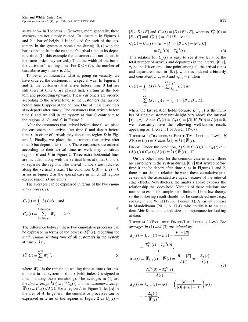
2.2. How the Averages in (1) Are Related
Figures 1 and 2 show how the three averages in (1) arerelated. These averages are related via L4t5 = �4t5SW4t5 ifthe system starts and ends empty, i.e., if R405 = L4t5 = 0,
Figure 1. The total work in the system during the inter-val [01 t] with edge effects: Including arrivalsbefore time 0 and departures after time t.
Futuret0
Arr
ival
num
ber
Past Present
Figure 2. Six regions: Waiting times (i) of customersthat both arrive and depart inside [01 t] (D),(ii) of arrivals before time 0 (A∪B∪C), and(iii) of departures after time t (C ∪E ∪ F ).
Arr
ival
num
ber
Futuret0Past Present
FE
D
CBA
A(t )
Kim and Whitt: Little’s LawOperations Research 61(4), pp. 1030–1045, © 2013 INFORMS 1033
as we show in Theorem 1. However, more generally, theseaverages are not simply related. To illustrate, in Figures 1and 2 a bar of height 1 is included for each of the cus-tomers in the system at some time during [01 t] with thebar extending from the customer’s arrival time to its depar-ture time. (In this example the customers do not depart inthe same order they arrived.) Thus the width of the bar isthe customer’s waiting time. For 0 ¶ s ¶ t, the number ofbars above any time s is L4s5.
To better communicate what is going on visually, wehave ordered the customers in a special way. In Figures 1and 2, the customers that arrive before time 0 but arestill there at time 0 are placed first, starting at the bot-tom and proceeding upwards. These customers are orderedaccording to the arrival time, so the customers that arrivedbefore time 0 appear at the bottom. One of these customersalso departs after time t. The customers that arrived beforetime 0 and are still in the system at time 0 contribute tothe regions A, B1 and C in Figure 2.
After the customers that arrived before time 0, we placethe customers that arrive after time 0 and depart beforetime t, in order of arrival; they constitute region D in Fig-ure 2. Finally, we place the customers that arrive aftertime 0 but depart after time t. These customers are orderedaccording to their arrival time as well; they constituteregions E and F in Figure 2. Three extra horizontal linesare included, along with the vertical lines at times 0 and t,to separate the regions. The arrival numbers are indicatedalong the vertical y axis. The condition R405 = L4t5 = 0arises in Figure 2 as the special case in which all regionsexcept region D are empty.
The averages can be expressed in terms of the two cumu-lative processes,
CL4t5≡
∫ t
0L4s5ds and
CW 4t5≡
R405+A4t5∑
k=R405+1
Wk1 t ¾ 00(4)
The difference between these two cumulative processes canbe expressed in terms of the process T
4r5W 4t5, recording the
total residual waiting time of all customers in the systemat time t, i.e.,
T4r5W 4t5≡
L4t5∑
k=1
W r1 tk 1 (5)
where W r1 tk is the remaining waiting time at time t for cus-
tomer k in the system at time t (with index k assigned attime t among those remaining). The averages in (1) arethe time average L4t5≡ t−1CL4t5 and the customer averageSW4t5 ≡ CW 4t5/A4t5. For a region A in Figure 2, let �A� bethe area of A. In general, the cumulative processes can beexpressed in terms of the regions in Figure 2 as CL4t5 =
�B ∪ D ∪ E� and CW 4t5 = �D ∪ E ∪ F �, whereas T4r5W 405 =
�B ∪C� and T4r5W 4t5= �C ∪ F �, so that
CL4t5−CW 4t5= �B� − �F � = �B ∪C� − �F ∪C�
= T4r5W 405− T
4r5W 4t50 (6)
This relation for CL4t5 is easy to see if we let � be thetotal number of arrivals and departures in the interval [01 t],�k be the kth-ordered time point among all the arrival timesand departure times in 601 t7, with ties indexed arbitrarilyand consistently, �0 ≡ 0 and ��+1 = t. Then
CL4t5≡
∫ t
0L4s5ds =
�+1∑
j=1
∫ �j
�j−1
L4s5ds
=
�+1∑
j=1
L4�j−154�j − �j−15= �B ∪D∪E�1
where the last relation holds because L4�j−15 is the num-ber of single-customer unit-height bars above the interval6�j−11 �j 7. Since CL4t5 = CW 4t5 = �D� if R405= L4t5= 0,we necessarily have the following well-known result,appearing as Theorem I of Jewell (1967).
Theorem 1 (Traditional Finite-Time Little’s Law). IfR405= L4t5= 0, then L4t5= �4t5SW4t5.
Proof. Under the condition, L4t5 ≡ CL4t5/t = CW 4t5/t =
4A4t5/t54CW 4t5/A4t55≡ �4t5SW4t5. �On the other hand, for the common case in which there
are customers in the system during [01 t] that arrived beforetime 0 and/or depart after time t, as in Figures 1 and 2,there is no simple relation between these cumulative pro-cesses and the associated averages, because of the intervaledge effects. Nevertheless, the analysis above exposes therelationship that does hold. Variants of these relations areneeded to establish sample-path limits in Little law theory,so the following result should not be considered new; e.g.,see Glynn and Whitt (1986, Theorem 1). A variant appearsin Mandelbaum (2011, p. 17.4), who credits it to his stu-dent Abir Koren and emphasizes its importance for lookingat data.
Theorem 2 (Extended Finite-Time Little’s Law). Theaverages in (1) and (3) are related by
ãL4t5 ≡ LW1�4t5− L4t5=�F � − �B�
t
=T
4r5W 4t5− T
4r5W 405
t3
ãW 4t5 ≡ SWL1�4t5− SW4t5=�B� − �F �
A4t5= −
ãL4t5
�4t5
=T
4r5W 405− T
4r5W 4t5
A4t53
(7)
ã�4t5 ≡ �L1W 4t5− �4t5=
(
�B� − �F �
�D� + �E� + �F �
)
�4t5
= −ãL4t5
SW4t51
Kim and Whitt: Little’s Law1034 Operations Research 61(4), pp. 1030–1045, © 2013 INFORMS
where �B� is the area of the region B in Figure 2 and T4r5W 4t5
is defined in (5).
Since we focus on inferences about the average waitbased on L4t5 and �4t5 using SWL1�4t5, we focus on ãW 4t5in (7). Given that the customers need not depart in the orderthey arrive and we only observe L4s5, 0 ¶ s ¶ t, the randomvariables T
4r5W 405 and T
4r5W 4t5 appearing in ãW 4t5 in (7) are
not directly observable; we only have partial informationabout these random variables.
2.3. Alternative Definitions to Force Equality:The Inside View
Denning and Buzen (1978), Little (2011), and others haveobserved that we can preserve the relation L4t5= �4t5SW4t5in Theorem 1 without any conditions on R405 and L4t5if we change the definitions. Equality can be achieved ingeneral if we assume that our entire view of the systemis inside the interval [01 t]. We see arrivals before time 0but only as arrivals appearing at time 0, and we see theportions of all waiting times only within the interval [01 t].To achieve the inside view, let A4i54t5 count the number ofnew arrivals plus the number of customers initially in thesystem, and let W
4i5k measure the waiting time inside the
interval [01 t]; i.e., let
A4i54t5≡R405+A4t51 t ¾ 01 and
W4i5k ≡ 4Dk ∧ t5− 4Ak ∨ 051 k¾ 11
(8)
where a∧b ≡ min 8a1 b9 and a∨b ≡ max 8a1 b9. Now con-sider the associated averages
�4i54t5≡ t−1A4i54t5 and SW 4i54t5≡
∑A4i54t5k=1 W
4i5k
A4i54t50 (9)
By an elementary modification of the proof of Theo-rem 1, we obtain the following “operational analysis” rela-tion. (The equality relation corresponds to the operationalLittle’s Law of Denning and Buzen 1978, p. 235; Little2011, Theorem LL.2.)
Theorem 3 (Finite-Time Version of Little’s Lawwith Altered Definitions). With the new definitions in(8) and (9), �4i54t5 ¾ �4t5, SW 4i54t5 ¶ SW4t51 and L4t5 =
�4i54t5SW 4i54t5.
Given that we only see inside the interval [01 t], thereduced waiting times are censored. Indeed, there is novalid upper bound on SW4t5 based on the inside view.Arrivals before time 0 can have occurred arbitrarily far inthe past prior to time 0, and customers present at time t canremain arbitrarily far into the future after time t. Any fur-ther properties of SW4t5 must depend on additional assump-tions about what happens outside the interval [01 t].
Even though the new definitions provide a good frame-work for checking the consistency of the data processing,and can be regarded as proper definitions, we advocate not
using this modification because it causes problems in inter-pretation. We think it is usually better to account for thefact that an important part of the story takes place out-side the interval [01 t], even if we do not see it all. Thealternative definitions in (8) also cause problems with themethod of batch means used to construct confidence inter-vals; see §3.4.
3. A Banking Call Center ExampleWe illustrate the statistical approach by considering datafrom a telephone call center of an American bank from thedata archive of Mandelbaum (2012). In 2001, this bankingcall center had sites in four states, which were integratedto form a single virtual call center. The virtual call centerhad 900–1,200 agent positions on weekdays and 200–500agent positions on weekends. The center processed about300,000 calls per day during weekdays, with about 60,000(20%) handled by agents, with the rest being served byintegrated voice response (IVR) technology. As in manymodern call centers, in this banking call center there weremultiple agent types and multiple call types, with a formof skill-based routing (SBR) used to assign calls to agents.
Because we are only concerned with estimation relatedto the three parameters L, �1 and W , we do not get involvedwith the full complexity of this system. For this paper, weuse data for one class of customers, denoted by “Summit,”for 18 weekdays in May 2001; the data used and the anal-ysis procedure are available from the authors’ Websites.Each working day covers a 17-hour period from 6 a.m. to11 p.m., referred to as [6123].
3.1. Sample Paths for a Typical Day
For some of the analyses, we will use a single day, Friday,May 25, 2001. Over this 17-hour period on that one daythere were 5,749 call arrivals (of this one type requesting anagent), of which 253 (4.4%) abandoned from queue beforestarting service. We do not include these abandonments inour analysis. Figures 3 and 4 show plots of the total numberof arrivals into the queue (system), Aq4s5, and into service,Aser4s5, together with the total number of departures fromthe queue (system), Dq4s5, and from service, Dser4s5, allover the interval [01 s], 0 ¶ s ¶ t, first over the entire work-ing day [6123] and then over the hour [14115]. These arebased on the counts over one-second subintervals. Note thatthe four curves in Figure 3 are too close to discern due toshort waiting time (time in system, measured in minutes)relative to the time scale (hours). We see better when wezoom in, as in Figure 4.
From the first plot in Figure 3, we see that the arrivalrate is not stationary over the entire day (because theslope is not nearly constant), but it appears to be approx-imately stationary over the middle part of the day, e.g.,in the six-hour interval [10116]. When the arrival rate isnearly constant, so is the departure rate. The stationary-and-independent-increments property associated with a
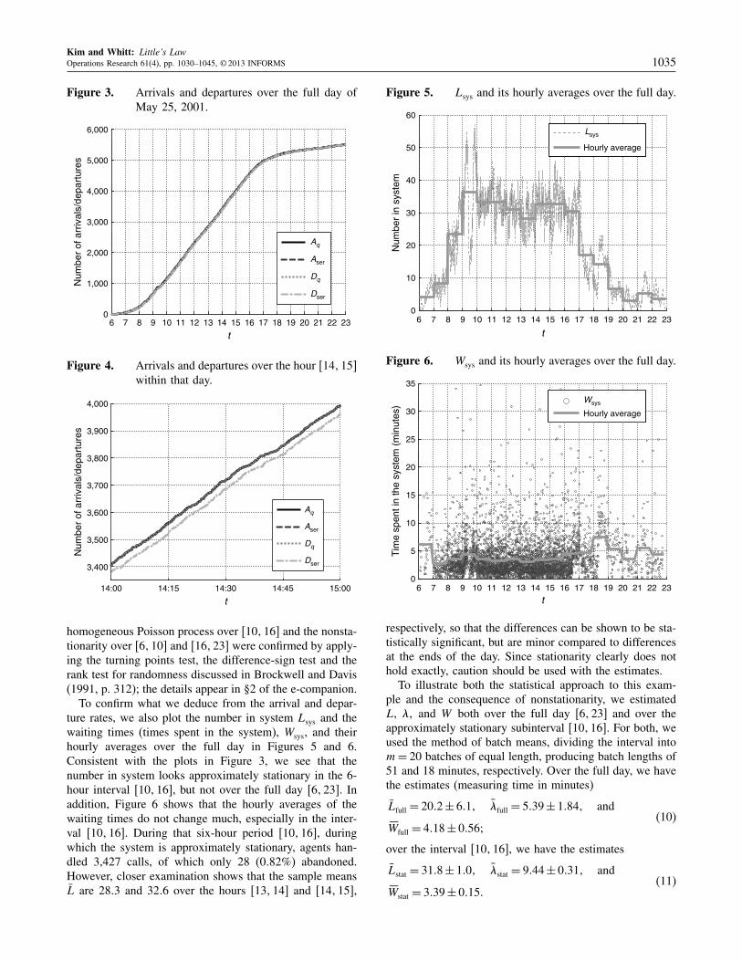
Kim and Whitt: Little’s LawOperations Research 61(4), pp. 1030–1045, © 2013 INFORMS 1035
Figure 3. Arrivals and departures over the full day ofMay 25, 2001.
6 7 8 9 10 11 12 13 14 15 16 17 18 19 20 21 22 230
1,000
2,000
3,000
4,000
5,000
6,000
t
Num
ber
of a
rriv
als/
depa
rtur
es
Aq
Aser
Dq
Dser
Figure 4. Arrivals and departures over the hour [14115]within that day.
14:00 14:15 14:30 14:45 15:00
3,400
3,500
3,600
3,700
3,800
3,900
4,000
t
Num
ber
of a
rriv
als/
depa
rtur
es
Aq
Aser
Dq
Dser
homogeneous Poisson process over [10116] and the nonsta-tionarity over [6110] and [16123] were confirmed by apply-ing the turning points test, the difference-sign test and therank test for randomness discussed in Brockwell and Davis(1991, p. 312); the details appear in §2 of the e-companion.
To confirm what we deduce from the arrival and depar-ture rates, we also plot the number in system Lsys and thewaiting times (times spent in the system), Wsys, and theirhourly averages over the full day in Figures 5 and 6.Consistent with the plots in Figure 3, we see that thenumber in system looks approximately stationary in the 6-hour interval [10116], but not over the full day [6123]. Inaddition, Figure 6 shows that the hourly averages of thewaiting times do not change much, especially in the inter-val [10116]. During that six-hour period [10116], duringwhich the system is approximately stationary, agents han-dled 3,427 calls, of which only 28 (0082%) abandoned.However, closer examination shows that the sample meansL are 2803 and 3206 over the hours [13114] and [14115],
Figure 5. Lsys and its hourly averages over the full day.
6 7 8 9 10 11 12 13 14 15 16 17 18 19 20 21 22 230
10
20
30
40
50
60
t
Num
ber
in s
yste
m
Lsys
Hourly average
Figure 6. Wsys and its hourly averages over the full day.
6 7 8 9 10 11 12 13 14 15 16 17 18 19 20 21 22 230
5
10
15
20
25
30
35
t
Tim
e sp
ent i
n th
e sy
stem
(m
inut
es)
Wsys
Hourly average
respectively, so that the differences can be shown to be sta-tistically significant, but are minor compared to differencesat the ends of the day. Since stationarity clearly does nothold exactly, caution should be used with the estimates.
To illustrate both the statistical approach to this exam-ple and the consequence of nonstationarity, we estimatedL, �1 and W both over the full day [6123] and over theapproximately stationary subinterval [10116]. For both, weused the method of batch means, dividing the interval intom= 20 batches of equal length, producing batch lengths of51 and 18 minutes, respectively. Over the full day, we havethe estimates (measuring time in minutes)
Lfull = 2002 ± 6011 �full = 5039 ± 10841 and
SWfull = 4018 ± 00563(10)
over the interval [10116], we have the estimates
Lstat = 3108 ± 1001 �stat = 9044 ± 00311 and
SWstat = 3039 ± 00150(11)
Kim and Whitt: Little’s Law1036 Operations Research 61(4), pp. 1030–1045, © 2013 INFORMS
For each estimate in (10) and (11), we also includethe halfwidth of the 95% confidence interval, estimatedas described in §4.3. We draw the following conclu-sions: (i) the confidence intervals tell us more than theaverages alone, (ii) paying attention to stationarity is impor-tant, (iii) the halfwidths themselves reveal the nonsta-tionarity, because we get far smaller halfwidths with theshorter subinterval [10116], and (iv) since the mean wait-ing time is much less than the batch length, the number ofbatches is not grossly excessive (but that requires furtherexamination).
3.2. Supporting Call Center Simulation Models
Many-server systems such as call centers are characterizedby having many servers working independently in paral-lel. In such systems (if managed properly), the waitingtimes in queue tend to be short compared to the servicetimes, and the service times tend to be approximately i.i.d.and independent of the arrival process. Thus, it is nat-ural to use an idealized infinite-server paradigm, involv-ing an infinite-server (IS) model with i.i.d. service timesindependent of the arrival process to approximately ana-lyze statistical methods. Because the service times coincideexactly with the waiting times in the IS model, the waitingtimes are i.i.d. with constant mean E6S7, even though weare considering a nonstationary setting. That often holdsapproximately in service systems, as illustrated by our callcenter example.
For the call center, we have data on the arrival timesand waiting times as well as the number in system L4s5,0 ¶ s ¶ t, but we do not have data on the staffing andthe complex call routing. Thus, as suggested in §1.2.2, toevaluate the estimation procedures, we simulate the single-class, single-service-pool Mt/GI/� IS model and asso-ciated Mt/GI/st models with time-varying staffing levelschosen to yield good performance, exploiting the squareroot staffing (SRS) formula s4t5 ≡ m4t5+�
√
m4t5, wherem4t5 is the offered load, the time-varying mean number ofbusy servers in the IS model, as in Jennings et al. (1996).As described in §3.1 of the e-companion, we fit the arrivalrate function to a continuous piecewise-linear function,with one increasing piece over [6110] starting at 0, a con-stant piece over [10116], and two decreasing linear piecesover [16118] and [18123], the first steeper and the secondending at 0. We then simulated a nonhomogeneous Poissonarrival process with this arrival rate function. We assumedthat all the service times were i.i.d., with a distributionobtained to match the observed waiting time distribution.A lognormal distribution with mean 3038 and squared coef-ficient of variation c2
s = 1002 was found to be a good fit,but an exponential distribution with that mean (and c2
s = 1)was also a good approximation, and so was used, becauseit is easier to analyze (see §3.2 of the e-companion). TheIS model was simulated with that fitted arrival rate functionand service-time distribution. The offered load m4t5 wasalso computed by formulas (6) and (7) of Jennings et al.
(1996), drawing on Eick et al. (1993b); then the staffingfunction s4t5 was determined by the SRS formula using arange of quality-of-service (QoS) parameters � (see §3.3 ofthe e-companion). We simulated 1,000 independent repli-cations of each of these models to study how the meth-ods to estimate confidence intervals performed. In the nextsubsection, we report results from simulation experimentsshowing that the finite-server models perform much likethe IS model.
3.3. Confidence Intervals for the CallCenter Data and Simulation
We applied the method of batch means to estimate con-fidence intervals for the parameters L, �1 and W usingthe direct sample averages from (1) plus indirect estimateSWL1�4t5 from (3) for the time interval [10116] over whichthe system is approximately stationary. (For both the callcenter data and the simulation model, we observe the wait-ing times, but we examine the alternative estimator SWL1�4t5from (3) to see how it would perform if we could notobserve the waiting times.)
We also consider the idealized Mt/M/� and Mt/M/stsimulation models introduced in §3.2 and explained indetail in §3 of the e-companion. The estimation results areshown in Table 1. Additional results with more values ofm appear in Kim and Whitt (2012, Tables 4–9).
For large QoS parameter �, e.g., � ¾ 200, the perfor-mance in the finite-server model is essentially the same asin the associated IS model, as can be seen from Table 1.However, as � decreases, more customers have to waitbefore starting service. Thus, the estimated mean waitingtime increases from 3038 in the IS model to 3039 and 3044,respectively, for � = 105 and 100, respectively. Similarly,the estimated mean number in the system increases from3105 to 3106 and 3201 for these same cases. Of specialinterest is the confidence interval (CI) coverage in the sim-ulations based on 1,000 replications. Table 1 shows it isexcellent for all values of m, being very close to the tar-get 9500%, for all � ¾ 105. However, we see a drop incoverage for � = 1. Thus, to be conservative, we advo-cate using for the call center model the largest estimatedCI, which usually should be associated with the smallestnumber of batches m = 5 for the call center data. Overall,Table 1 shows that the indirect estimator SW
4m5L1�4t5 behaves
very much the same as the direct estimator SW4t5. Indeed,that is consistent with the theory and other experiments inthis paper.
To illustrate what happens with a shorter sample-pathsegment, we consider the interval [14115]. Table 2 showsthe corresponding estimates for the IS model and the callcenter. Additional results with more values of m appear inTables 10 and 11 of Kim and Whitt (2012). In this case,m = 5, 10, and 20 corresponds to 5 batches of 12 min-utes, 10 batches of 6 minutes, and 20 batches of 3 minutes,respectively. The CI coverage is again excellent for the ISmodel for all cases. However, since the mean waiting time
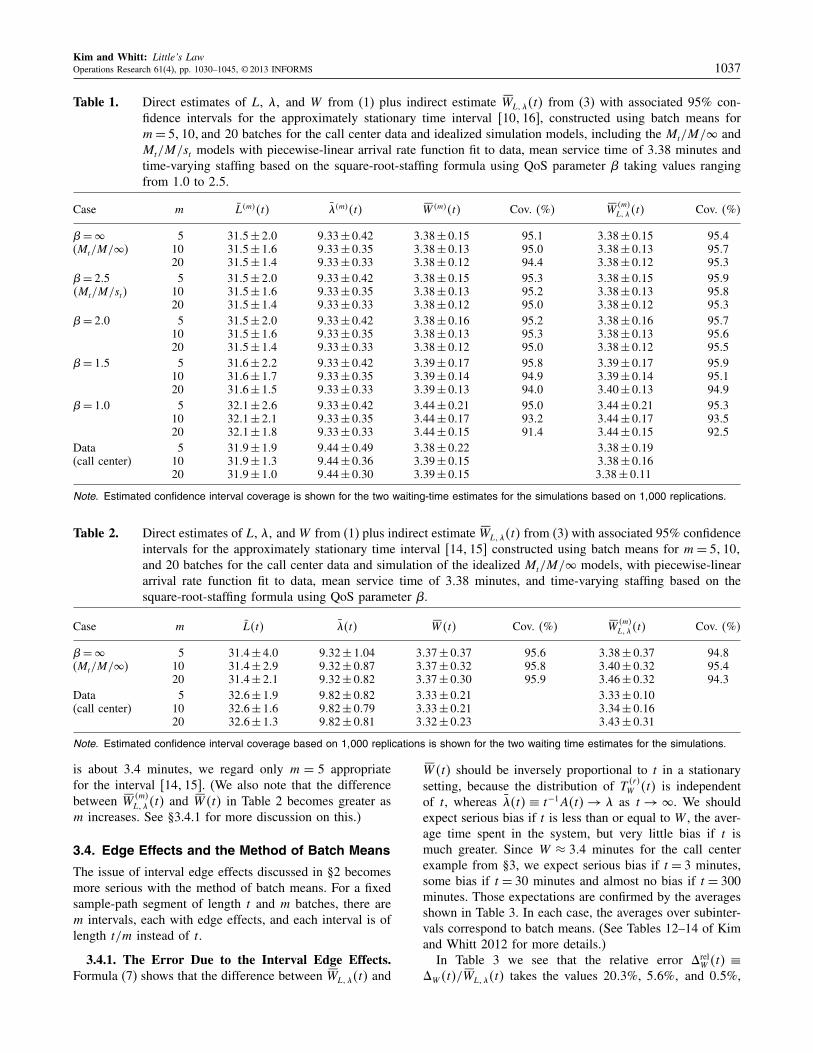
Kim and Whitt: Little’s LawOperations Research 61(4), pp. 1030–1045, © 2013 INFORMS 1037
Table 1. Direct estimates of L, �1 and W from (1) plus indirect estimate SWL1�4t5 from (3) with associated 95% con-fidence intervals for the approximately stationary time interval 6101167, constructed using batch means form= 51101 and 20 batches for the call center data and idealized simulation models, including the Mt/M/� andMt/M/st models with piecewise-linear arrival rate function fit to data, mean service time of 3038 minutes andtime-varying staffing based on the square-root-staffing formula using QoS parameter � taking values rangingfrom 100 to 205.
Case m L4m54t5 �4m54t5 SW 4m54t5 Cov. 4%5 SW4m5L1�4t5 Cov. 4%5
�= � 5 3105 ± 200 9033 ± 0042 3038 ± 0015 9501 3038 ± 0015 9504(Mt/M/�) 10 3105 ± 106 9033 ± 0035 3038 ± 0013 9500 3038 ± 0013 9507
20 3105 ± 104 9033 ± 0033 3038 ± 0012 9404 3038 ± 0012 9503�= 205 5 3105 ± 200 9033 ± 0042 3038 ± 0015 9503 3038 ± 0015 95094Mt/M/st5 10 3105 ± 106 9033 ± 0035 3038 ± 0013 9502 3038 ± 0013 9508
20 3105 ± 104 9033 ± 0033 3038 ± 0012 9500 3038 ± 0012 9503�= 200 5 3105 ± 200 9033 ± 0042 3038 ± 0016 9502 3038 ± 0016 9507
10 3105 ± 106 9033 ± 0035 3038 ± 0013 9503 3038 ± 0013 950620 3105 ± 104 9033 ± 0033 3038 ± 0012 9500 3038 ± 0012 9505
�= 105 5 3106 ± 202 9033 ± 0042 3039 ± 0017 9508 3039 ± 0017 950910 3106 ± 107 9033 ± 0035 3039 ± 0014 9409 3039 ± 0014 950120 3106 ± 105 9033 ± 0033 3039 ± 0013 9400 3040 ± 0013 9409
�= 100 5 3201 ± 206 9033 ± 0042 3044 ± 0021 9500 3044 ± 0021 950310 3201 ± 201 9033 ± 0035 3044 ± 0017 9302 3044 ± 0017 930520 3201 ± 108 9033 ± 0033 3044 ± 0015 9104 3044 ± 0015 9205
Data 5 3109 ± 109 9044 ± 0049 3038 ± 0022 3038 ± 0019(call center) 10 3109 ± 103 9044 ± 0036 3039 ± 0015 3038 ± 0016
20 3109 ± 100 9044 ± 0030 3039 ± 0015 3038 ± 0011
Note. Estimated confidence interval coverage is shown for the two waiting-time estimates for the simulations based on 11000 replications.
Table 2. Direct estimates of L, �1 and W from (1) plus indirect estimate SWL1�4t5 from (3) with associated 95% confidenceintervals for the approximately stationary time interval 6141157 constructed using batch means for m = 51101and 20 batches for the call center data and simulation of the idealized Mt/M/� models, with piecewise-lineararrival rate function fit to data, mean service time of 3038 minutes, and time-varying staffing based on thesquare-root-staffing formula using QoS parameter �.
Case m L4t5 �4t5 SW4t5 Cov. 4%5 SW4m5L1�4t5 Cov. 4%5
�= � 5 3104 ± 400 9032 ± 1004 3037 ± 0037 9506 3038 ± 0037 9408(Mt/M/�) 10 3104 ± 209 9032 ± 0087 3037 ± 0032 9508 3040 ± 0032 9504
20 3104 ± 201 9032 ± 0082 3037 ± 0030 9509 3046 ± 0032 9403Data 5 3206 ± 109 9082 ± 0082 3033 ± 0021 3033 ± 0010(call center) 10 3206 ± 106 9082 ± 0079 3033 ± 0021 3034 ± 0016
20 3206 ± 103 9082 ± 0081 3032 ± 0023 3043 ± 0031
Note. Estimated confidence interval coverage based on 11000 replications is shown for the two waiting time estimates for the simulations.
is about 304 minutes, we regard only m = 5 appropriatefor the interval [14115]. (We also note that the differencebetween SW
4m5L1�4t5 and SW4t5 in Table 2 becomes greater as
m increases. See §3.4.1 for more discussion on this.)
3.4. Edge Effects and the Method of Batch Means
The issue of interval edge effects discussed in §2 becomesmore serious with the method of batch means. For a fixedsample-path segment of length t and m batches, there arem intervals, each with edge effects, and each interval is oflength t/m instead of t.
3.4.1. The Error Due to the Interval Edge Effects.Formula (7) shows that the difference between SWL1�4t5 and
SW4t5 should be inversely proportional to t in a stationarysetting, because the distribution of T
4r5W 4t5 is independent
of t, whereas �4t5 ≡ t−1A4t5 → � as t → �. We shouldexpect serious bias if t is less than or equal to W , the aver-age time spent in the system, but very little bias if t ismuch greater. Since W ≈ 304 minutes for the call centerexample from §3, we expect serious bias if t = 3 minutes,some bias if t = 30 minutes and almost no bias if t = 300minutes. Those expectations are confirmed by the averagesshown in Table 3. In each case, the averages over subinter-vals correspond to batch means. (See Tables 12–14 of Kimand Whitt 2012 for more details.)
In Table 3 we see that the relative error ãrelW 4t5 ≡
ãW 4t5/SWL1�4t5 takes the values 2003%, 506%1 and 005%,
Kim and Whitt: Little’s Law1038 Operations Research 61(4), pp. 1030–1045, © 2013 INFORMS
Table 3. Comparison of the direct and indirect estimators SW4t5 and SWL1�4t5 for three values of t: 3, 301 and 300 minutesfor the data from §3.
t SW4t5 SWL1�4t5 �ãW 4t5� ãrelW 4t5 (%) �U � �A� (%) �B� (%) �C� (%) �D� (%) �E� (%) �F � (%) �F � − �B� (%)
3 3032 3043 00713 2003 311 3408 1905 1403 301 809 1904 60330 3080 3080 00241 506 11101 907 902 000 6208 904 808 405300 3044 3044 00016 005 91754 104 102 000 9409 102 103 004
Note. Averages are given for the 20 subintervals of 6141157 for t = 3 minutes, for the 20 subintervals of 681187 for t = 30 minutes and for thefour overlapping five-hour subintervals of 691177, from 691147 to 6121177, for t = 300 minutes.
respectively, for t = 3, 301 and 300 minutes. For the regionsin Figure 2, for t ¾ 30 minutes, we see that �C� = 0, theareas of regions B, C, E1 and F are approximately indepen-dent of t, while the area of D is proportional to t. Table 3shows the area of the union of all six regions, U ≡ A ∪
B ∪C ∪D ∪ E ∪ F , and the percentages of that total areamade up by each of the six regions, as well as �F � − �B�.The simple case occurs when region D dominates the sixregions. The percentage of the total area provided by D is9409% for t = 300 minutes, 6208% for t = 30 minutes, and301% for t = 3 minutes.
3.4.2. Additional Error from the Altered Definitions.The altered definitions in §2.3 become more unattractivewith batch means, because the shorter intervals distort themeaning even more. The average truncated waiting timesSWc4t5 in (9) tend to be even less than the true average wait-ing times W , whereas the average augmented arrivals �i4t5in (9) tend to be even more than the true average arrivalrate �. The altered definitions lead to double counting forarrivals. Customers that are in the system during more thanone interval are counted as arrivals in all these intervals.
To illustrate, we consider the call center data over theinterval [10116]. Without using batches, we have �4t5 =
9044 arrivals per minute and SW4t5= 3038 minutes, whereasthe estimators using the altered definitions in (9) are �i4t5=
9055 and SWc4t5 = 3033. With m batches, 1 ¶ m ¶ 20, theestimator �4t5 is unchanged and the estimator SW4t5 dif-fers by only 00001 from the original value of 3038 form= 1. In contrast, �i4t5 assumes the values 9055, 9088,100331 and 11016 for m = 1, 5, 10, and 20, respectively.Similarly, SWc4t5 assumes the values 3033, 3022, 3009, and2086 for m = 1, 5, 10, and 20, respectively. For m = 20,the errors in �i4t5 and SWc4t5 are 18% and 15%, respec-tively. When confidence intervals are formed based onbatch means (for nonnegligible m), the systematic errorscaused by the altered definition far exceed the halfwidth ofthe confidence interval. Hence, we recommend not usingthe modified definitions in (9).
4. Confidence Intervals: Theory andMethodology
We now consider how to apply the estimator SWL1�4t5 in (3)to estimate a confidence interval (CI) for W in a stationarysetting and for E6SW4t57 in a nonstationary setting, without
observing the waiting times. We will be using statisticalmethods commonly used in simulation experiments. How-ever, unlike simulation, we anticipate that system data islikely to be limited, so we may not be able to achieve highprecision. Nevertheless, we want to have some idea howwell we know the estimated values. With that in mind, wesuggest applying standard statistical methods. To evaluatehow well these statistical procedures should perform, e.g.,to verify that CI coverage should be approximately as spec-ified, we advocate studying associated idealized simulationmodels of the system more closely as suggested in §1.2.2and as illustrated in §3.2.
For the common case in which we have only a singlesample-path segment, we advocate applying the method ofbatch means, as specified in §4.3. That method dependson the batch means being approximately i.i.d. and nor-mally distributed. We point out that there is a risk thatthese assumptions may not be justified, so that estimatedCIs should be used with caution. We suggest using multi-ple i.i.d. replications of the supporting simulation model toconfirm these properties and evaluate the confidence inter-val coverage. If these standard methods do not perform wellfor the supporting simulation models, then we can considermore sophisticated estimation methods, as in Alexopouloset al. (2007), Tafazzoli et al. (2011), Tafazzoli and Wilson(2011) and references therein.
4.1. A Ratio Estimator
In both stationary and nonstationary settings, a CI (inter-val estimate) for E6SW4t57 without observing the waitingtimes can be obtained using SWL1�4t5 if we can apply thefollowing theorem, implementing the delta method; seeAsmussen and Glynn (2007, §III.3 and Proposition §IV.4.1)for related results.
Theorem 4 (Asymptotics for the Ratio of Low-Variability Positive Normal Random Variables). Ifthere is a sequence of systems indexed by n such that√n4L4n54t5−L1 �4n54t5−�5
=⇒ N401è5 in �2 as n→ �1 (12)
where L and � are positive real numbers and N401è5 is amean-zero bivariate Gaussian random vector with variancevector 4�2
L1�2�5 and covariance �2
L1�, and SW 4n54t5 satisfies
SW 4n54t5/SW4n5L1�4t5 =⇒ 1 as n→ �1 (13)
Kim and Whitt: Little’s LawOperations Research 61(4), pp. 1030–1045, © 2013 INFORMS 1039
for SW4n5L1�4t5≡ L4n54t5
/
�4n54t5, then√n4SW 4n54t5− 4L/�55
=⇒ N401�2W 5 in � as n→ � (14)
for
�2W =
1�2
(
�2L −
2L�2L1�
�+
L2�2�
�2
)
0 (15)
Proof. Apply a Taylor expansion with the functionf 4x1 y5≡ x/y, having first partial derivatives fx = 1/y andfy = −x/y2, to get
L4n54t5
�4n54t5=
L
�+
L4n54t5−L
�−
L4�4n54t5−�5
�2
+ o(
max 8�L4n54t5−L�1 ��4n54t5−��9)
1 (16)
so that√n(
SW4n5L1�4t5− 4L/�5
)
=
√n4L4n54t5−L5
�−
√nL4�4n54t5−�5
�2
+ o415 as n→ �1 (17)
from which (14) follows, given (12) and (13). �We can apply the theorem if our system can be regarded
as system n for n sufficiently large that we can replacethe limits with approximate equality. The approximate con-fidence interval estimate for E6SW 4n54t57 would then be6SW
4n5L1�4t5−1096�W /
√n1 SW
4n5L1�4t5+1096�W /
√n7, where �W
is the square root of the variance �2W in (15). Since the
variance �2W in (15) is typically unknown, we must esti-
mate it. That can be done by inserting estimates for allthe components of (15). Assuming that the estimates con-verge as n → �, we still have asymptotic normality withthe estimated values of the variance �2
W .The sequence of systems indexed by n satisfying con-
dition (12) in Theorem 4 can arise in two natural ways:First, condition (12) is typically satisfied if the averagesare collected from a single observation over successivelylonger time intervals in a stationary environment, i.e., if tis allowed to grow with n, with tn → �. Then, of course,E6SW 4n54t57 → W as n → �, and we are simply estimat-ing W . Second, whether or not there is a stationary envi-ronment, condition (12) is satisfied if the averages indexedby n correspond to averages taken over n multiple inde-pendent samples for a fixed interval [01 t]. The second caseis important for the common case of service systems withstrongly time-varying arrival rates over each day, providedthat multiple days can be regarded as i.i.d. samples.
Condition (13) in Theorem 4 is of course also satisfiedif the averages are collected from a single observation oversuccessively longer time intervals in a stationary environ-ment. However, condition (13) may well not be satisfied,even approximately, if the averages indexed by n corre-spond to averages taken over n multiple independent sam-ples for a fixed interval [01 t], because the bias may be sig-nificant, and it does not go away with increasing n; see §5.
4.2. The Supporting Central Limit Theorem in aStationary Setting
With one sample-path segment, we suggest applying themethod of batch means. A partial basis for that is the cen-tral limit theorem (CLT) version of Little’s Law in Glynnand Whitt (1986) and Whitt (2012). To apply it, we assumethat the system is approximately stationary over the des-ignated subinterval [01 t]. Hence we regard the finite aver-ages in (1) as estimators of the unknown parameters L, �,and W . The CLT states that, under very general regularityconditions,
(
L4t51 �4t51 W 4t51 LW1�4t51 �L1W 4t51 WL1�4t5)
=⇒ 4XL1X�1XW 1XL1X�1XW 5 in �6 (18)
as t → �, where
(
L4t51 �4t51 W 4t5)
≡√t(
L4t5−L1 �4t5−�1 SW4t5−W)
1(
LW1�4t51 �L1W 4t51 WL1�4t5)
≡√t(
LW1�4t5−L1 �L1W 4t5−�1 SWL1�4t5−W)
1
(19)
with the averages given in (1) and (3), and the limiting ran-dom vector 4XL1X�1XW 5 is an essentially two-dimensionalmean-zero multivariate Gaussian random vector with XW =
�−14XL −WX�55, so that the variance and covariance termsare related by
�2W ≡ Var4XW 5=E6X2
W 7
= �−24�2L − 2W�2
�1L +W 2�2�51
�2L1W ≡ Cov4XL1XW 5=E6XLXW 7
= �−14�2L −W�2
�1L51(20)
�2W1� ≡ Cov4XW 1X�5=E6XWX�7
= �−14�2�1L −W�2
�50
Note that �2W in (20) agrees with (15).
Under general regularity conditions (essentially, ift1/2T
4r5W 4t5⇒ 0 for T 4r5
W 4t5 in (5)), a functional central limittheorem (FCLT) generalization of the joint CLT in (18) isvalid if a FCLT is valid in �2 for any two of the first threecomponents. For example, it suffices to start with (FCLTgeneralization of) the bivariate CLT
√t4L4t5−L1 �4t5−�5
=⇒ 4XL1X�5 in �2 as t → �1 (21)
where the limit 4XL1X�5 is a bivariate mean-zero Gaussianrandom vector with variances �2
� , �2L1 and covariance
�2�1L. Natural sufficient conditions are based on regenera-
tive structure for the stochastic process 8L4t52 t ¾ 09, asin Asmussen (2003, §VI.3) and Glynn and Whitt (1987).
Kim and Whitt: Little’s Law1040 Operations Research 61(4), pp. 1030–1045, © 2013 INFORMS
We directly assume that the limit in (18) is valid, and dis-cuss how to apply it. Note that condition (21) coincideswith condition (12) in Theorem 4, but now the conclusiondirectly gives a CLT for SW4t5 as well as for SWL1�4t5.
The form of the limit in (18) implies that the alternativeestimators LW1�4t5, �L1W 4t51 and SWL1�4t5 in (3) not onlyconverge to the same limits L, � and W just as the nat-ural estimators L4t5, �4t51 and SW4t5 in (1) do, but alsothe corresponding CLT-scaled random variables are asymp-totically equivalent as well, i.e., �4L4t51 �4t51 W 4t55 −
4LW1�4t51 �L1W 4t51 WL1�4t55� ⇒ 0 as t → �, where � · � isthe Euclidean norm on �3.
In summary, the CLT version of L= �W implies that theasymptotic efficiency (halfwidth of confidence intervals forlarge sample sizes) is the same for the alternative estimatorsin (3) as it is for the natural estimators in (1) (in a stationarysetting). However, if one of the parameters happens to beknown in advance, one estimator can be more efficient thanthe other; see Glynn and Whitt (1989). For example, withsimulation, the arrival rate is typically known in advance.
4.3. Estimating Confidence Intervals by theMethod of Batch Means
Assuming that the conditions for the CLT in the previ-ous section are satisfied, given the sample-path segments84A4s51L4s552 0 ¶ s ¶ t9 and 8Wk2 R405+ 1 ¶ k¶ R405+
A4t59 over the time interval [01 t] (or only two of thesethree segments), we can use m batches based on mea-surements over the m subintervals 64k − 15t/m1kt/m7,1 ¶ k¶m. To define the batch averages, let Rk ≡R4kt/m5,the number of customers remaining in the system attime kt/m from among those that arrived previously. LetAk4t1m5, Lk4t1m5, and SWk4t1m5 denote the averages overthe interval 64k− 15t/m1kt/m7, i.e.,
Ak4t1m5≡ 4m/t5Ak4t1m51
Lk4t1m5≡ 4m/t5Lk4t1m51
SWk4t1m5≡ 41/Ak4t1m55Wk4t1m51
Ak4t1m5≡A4kt/m5−A44k− 15t/m51
Lk4t1m5≡∫ kt/m
4k−15t/mL4s5ds1 Wk4t1m5≡∑Rk−1+Ak4t1m5
j=Rk−1+1 Wj 0
(22)
The FCLT version of the CLT in the previous sec-tion implies that, as t → �, the vector of scaled batchmeans
√t/m4Ak4t1m5 − �1 Lk4t1m5 − L1 SWk4t1m5 − W5,
1 ¶ k¶m, are asymptotically m i.i.d. mean-zero Gaussianrandom vectors with variances �2
� , �2L, and �2
W , and covari-ances �2
L1�, �2�1W 1 and �2
L1W . By Theorem 4, as t → �, theassociated scaled vector
√t/m4SWL1�1k4t1m5−W5, 1 ¶ k¶
m, are asymptotically m i.i.d. mean-zero random variableswith variance �2
W in (15). Hence, as t → �, also
∑mk=14SWL1�1k4t1m5− SW
4m5L1�4t55
√
S24m54t5/m
=⇒ tm−11 (23)
where tm−1 is a random variable with the Student t distri-bution with m− 1 degrees of freedom,
SW4m5L1�4t5≡
1m
m∑
k=1
SWL1�1k4t1m5 and
S24m54t5≡
1m− 1
m∑
k=1
4SWL1�1k4t1m5− SW4m5L1�4t55
20
(24)
Thus,[
SW4m5L1�4t5−
t000251m−1S4m54t5√m
1 SW4m5L1�4t5+
t000251m−1S4m54t5√m
]
is an approximate 95% confidence interval for W based onthe t distribution and the average SW
4m5L1�4t5 of batch means.
Of course, the same procedure applies to other averages ofbatch means as well.
It remains to choose the number of batches, m. Since weobtain larger batch sizes, and thus more nearly approximatethe asymptotic condition t → �, if we make m small, weadvocate keeping it relatively small, e.g., m= 5. Neverthe-less, in our examples we consider a range of m values.
5. Estimating and Reducing the BiasWe now discuss ways to estimate and reduce the bias inthe estimator SWL1�4t5 in (3) as an estimator for E6SW4t57for SW4t5 in (1). In doing so, we are primarily concernedwith nonstationary settings. In stationary settings, SW4t5 in(1) is typically a biased estimator of W , whereas SWL1�4t5is typically a biased estimator of both W and E6SW4t57, butthese biases are less likely to be serious, e.g., see §5.4.
An important conclusion from our analysis is that thebias depends on the underlying model. We demonstrateby considering two idealized paradigms: the infinite-serverand single-server paradigms. We emphasize the infinite-server paradigm, which often is appropriate for call centers.In §5.4, we show that the bias in SW4t5 for estimating Wtends to be negligible in the infinite-server paradigm.
5.1. Bias in SWL1�4t5 as an Estimator of theExpected Average Wait E6SW4t57
Since the bias in SWL1�4t5 as an estimator for E6SW4t57is E6ãW 4t57 for ãW 4t5 ≡ SWL1�4t5 − SW4t5 in (7), we canapply Theorem 2 to obtain an exact expression for the biasE6ãW 4t57. We also give the conditional bias E6ãW 4t5 � Ot7given the observed data over the interval [01 t], which weassume is O4t5 ≡ 4t1 L4t51 �4t51R4051L4t55, from whichwe can also deduce A4t5. We use the conditional bias tocreate a refined estimator given the observed data.
Corollary 1 (Exact Bias and Conditional Bias). Thebias in SWL1�4t5 in (3) as an estimator for E6SW4t57 for SW4t5in (1) is E6ãW 4t57 = E6E6ãW 4t5 � O4t577, where ãW 4t5is given in (7), the vector of observed data is O4t5 ≡
4t1 L4t51 �4t51R4051L4t55 and the conditional bias is
E6ãW 4t5 �Ot7=
∑R405k=1 E6W
r10k �Ot7−
∑L4t5k=1E6W
r1 tk �Ot7
A4t50 (25)
Proof. Apply Theorem 2 using (5). �
Kim and Whitt: Little’s LawOperations Research 61(4), pp. 1030–1045, © 2013 INFORMS 1041
5.2. Two Approximations
The bias in Corollary 1 is not easy to analyze. Giventhat 4R4051L4t51A4t55 is observed, it remains to estimatethe conditional residual waiting times E6W r10
k � Ot7, 1 ¶k ¶ R405, and E6W r1 t
k � Ot7, 1 ¶ k ¶ L4t5. The conditionalexpectations E6W r10
k � Ot7 are complicated, because we areconditioning on events in the future after the observationtime 0. Thus, we develop two approximations and thenshow that they apply to the infinite-server paradigm.
5.2.1. Simplification from the Bias ApproximationAssumption. As t increases, we expect the “initial edgeeffect” 8R4051W r10
k 31 ¶ k ¶ R4059 to be approximatelyindependent of the “terminal edge effect” 8L4t51W r1 t
k 31 ¶k¶ L4t59 and the total number of arrivals A4t5. With that inmind, we use the following approximation, which primarilymeans that we are assuming that t is sufficiently large.
Bias Approximation Assumption 4BAA5. For O4t5 ≡
4t1 L4t51 �4t51R4051L4t55, t ¾ 0,
E6W r10k � Ot7≈E6W r10
k �R40571 0 ¶ k¶R4051 and
E6W r1 tk � Ot7≈E6W r1 t
k � L4t571 0 ¶ k¶ L4t50
Invoking the BAA, we obtain the following approxima-tion directly from Corollary 1:
E6ãW 4t5 � Ot7
≈
∑R405k=1 E6W
r10k �R4057−
∑L4t5k=1 E6W
r1 tk � L4t57
A4t50 (26)
We think that BAA is reasonable if t is suffi-ciently large. That is easy to see for stationary models,because then as t→� (i) L4t5→L and �4t5→� and(ii) under regularity conditions (e.g., regenerative structure),8R4051W r10
k ; 1 ¶ k¶R4059 will be asymptotically indepen-dent of 8L4t51W r1 t
k ; 1 ¶ k¶ L4t59.
5.2.2. Using SWL1�4t5 to Estimate the Residual Wait-ing Times. We can obtain an applicable estimate ofthe conditional bias E6ãW 4t5 � Ot7 in (25) if we esti-mate all the remaining conditional waiting times by theobserved SWL1�4t5. In doing so, we are ignoring the inspec-tion paradox (since these are remainders of waiting timesin progress), the model structure and the available informa-tion O4t5. This step is likely to be justified approximately ifthe distribution of the waiting times is nearly exponential.
That step yields the approximation
E6ãW 4t5 � Ot7≈4R405−L4t55SWL1�4t5
A4t5for
O4t5≡ 4R4051L4t51 L4t51 �4t550 (27)
We can apply approximation (27) to obtain the new candi-date refined estimator of E6SW4t57, exploiting the observedvector 4R4051L4t51A4t55:
SWL1�1 r4t5≡ SWL1�4t5−E6ãW 4t5 � Ot7
≈ SWL1�4t5
(
1 −R405−L4t5
A4t5
)
0(28)
(The refined estimator SWL1�1 r4t5 in (28) is a candidaterefinement of the indirect estimator SWL1�4t5 (3).) The asso-ciated approximate relative conditional bias is thus
E6ãrelW 4t5 � O4t57≡
E6ãW 4t5 � Ot7
E6SW4t57≈
E6ãW 4t5 � Ot7
SWL1�4t5
≈R405−L4t5
A4t50 (29)
In the next section we show that the analysis in (27)–(29)can be supported theoretically in the infinite-serverparadigm when the waiting times are exponential, so wepropose the refined estimator in (28) as a candidate estima-tor for many-server systems. However, the crude analysisabove is not justified universally; e.g., it is not good for thesingle-server models, as we show in §5.5.
5.3. The Infinite-Server Paradigm
If, in addition to BAA, we consider the Gt/M/� IS modelwith exponential service times having mean E6S7, then (26)becomes
E6ãW 4t5 � Ot7≈ 4R405−L4t55E6S7/A4t50 (30)
Since the waiting times coincide with the service times inthe IS model, it is natural to use the observed SWL1�4t5 as aninitial estimate of E6S7. If we use SWL1�4t5 as an estimate ofE6S7 in (30), then the formula in (30) reduces to the biasapproximation in (27). Thus, under these approximations,the refined estimator (28) becomes unbiased. Hence, wepropose the refined estimator in (28) for light to moderatelyloaded many-server systems with service time-distributionsnot too far from exponential.
To better understand the consequence of nonexponentialservice times in the infinite-server paradigm, we now con-sider the Mt/GI/� IS model with nonexponential servicetimes. We assume that it starts empty at some time in thepast (possibly in the infinite past) having bounded time-varying arrival rate �4t5, i.i.d. service times, independentof the arrival process, with generic service-time S havingcdf G4x5 ≡ P4S ¶ x5 with E6S27 < � and thus the finite-squared coefficient of variation (SCV) c2
S ≡ Var4S5/E6S72.Let Gc4x5 ≡ 1 − G4x5 be the complementary cdf. Let Sebe an associated random variable with the associated sta-tionary excess or residual lifetime distribution,
P4Se ¶ x5≡1
E6S7
∫ x
0Gc4u5du and
E6Ske 7=
E6Sk+17
4k+ 15E6S70
(31)
For this IS model, we can characterize the conditionalexpected value of the remaining work T
4r5W 4t5 in (5) and (7)
given L4t5, but it requires the full waiting-time cdf G.
Kim and Whitt: Little’s Law1042 Operations Research 61(4), pp. 1030–1045, © 2013 INFORMS
Theorem 5 (Total Remaining Work for the Mt/GI/�Infinite-Server Model). For the Mt/GI/� model above,
E6T4r5W 4t5 � L4t57
=L4t5
∫ �
0 �4t − u5E6S − u3S > u7du
E6L4t571 (32)
for T4r5W 4t5 in (5), where E6S − u3S > u7 = E6S −
u � S > u7P4S > u5, E6S − u � S > u7 =∫ �
0 4Gc4x −
u5/Gc4u55dx, and
E6L4t57=∫ �
0�4t − u5Gc4u5du
=E6�4t − Se57E6S71 t ¾ 00 (33)
Proof. Conditional on L4t5 = n, the n customers remain-ing in service have i.i.d. service times distributed as St with
P4St > x5=
∫ �
0 �4t − u5P4S > x+ u5du
E6L4t571 (34)
for E6L4t57 given in (33), by Goldberg and Whitt (2008,Theorem 2.1), which draws on Eick et al. (1993a). Therethe system starts empty at time 0, but the result extendsto the present setting, given that we have assumed thatthe arrival rate function is bounded and E6S27 < �. Thesecond expression in (33) is given in Eick et al. (1993a,Theorem 1). �
If we now invoke the BAA for the Mt/GI/� model,then we obtain the approximation
E6ãW 4t5 �Ot7≈E6T
4r5W 405 �L4057−E6T
4r5W 4t5 �L4t57
A4t51 (35)
where (32) can be used to compute both terms in thenumerator.
In practice, we presumably would not know the fullservice-time cdf, so that the approximation in (35) basedon Theorem 5 would not appear to be very useful, but wenow show that it provides strong support for the refinedestimator in (28) if the service time is not too far fromexponential. For that purpose, we observe that the compli-cated formula above simplifies in special cases. First, forMt/M/�, formula (32) reduces to
E6T4r5W 4t5 � L4t57= L4t5E6S71
taking us back to (27). Second, for the stationary M/GI/�model starting empty in the infinite past, St in (34) is dis-tributed as Se in (31), so that formula (32) reduces to
E6T4r5W 4t5 � L4t57= L4t5E6Se7= L4t5E6S74c2
s + 15/2
and (35) reduces to
E6ãW 4t5 � Ot7= 4R405−L4t55E6S74c2s + 15/2A4t51
depending only on the first two moments of the distribution.This result for the stationary M/GI/� model applies
to the nonstationary Mt/GI/� system if the arrival rate is
nearly constant just prior to the two times 0 and t, wherewe would be applying Theorem 5. Thus, we conclude thatthis section provides strong support for the refined estima-tor SWL1�1 r4t5 in (28) in the common case where (i) thearrival rate changes relatively slowly compared to the meanservice time and (ii) the service-time SCV c2
s is not too farfrom 1, as is often the case in call centers, e.g., here (wherec2s = 10017) and in Brown et al. (2005). We could obtain a
further refinement if we could estimate the SCV c2s .
5.4. Bias of SW4t5 in the Infinite-Server Paradigm
We now observe that the bias of SW4t5 as an estimator of Wshould usually not be a major factor in the infinite-serverparadigm. We do so by showing that the bias is quantifi-ably small for an IS model. We use the Gt/GI/� modelwith general, possibly nonstationary, arrival counting pro-cess A. The key assumption is that the waiting times, whichcoincide with the service times, are i.i.d. with mean Wand independent of the arrival process. Using that indepen-dence, we can write
E6SW4t5 �A4t5 > 07=E6E6SW4t5 �A4t57 �A4t5 > 07
=E6W �A4t5 > 07=W0 (36)
Given that we have defined SW4t5 ≡ 0 when A4t5 = 0, wehave the following result.
Theorem 6 (Conditional Bias of the Average Wait-ing Time in the Gt/GI/� Model). For the Gt/GI/�infinite-server model, having i.i.d. service times withmean W , that are independent of a general arrival process,
E6SW4t57=WP4A4t5 > 050 (37)
For a stationary Poisson arrival process with rate �,W −E6SW4t57=We−�t , t ¾ 0.
5.5. The Single-Server Paradigm
To show that the refined estimator SWL1�1 r4t5 in (28) is notalways good and that the bias can be analyzed exactlyin some cases and can be significant, we now considera single-server model. Let L4t5 be the number of cus-tomers waiting in queue in a single-server Gt/GI/1 queue-ing model with unlimited waiting space and the first-comefirst-served service discipline, with a general arrival processpossibly having a time-varying arrival-rate function �4t5and service times Si that are independent and identicallydistributed (i.i.d.) and independent of the arrival process,each distributed as a random variable S having cdf G4x5.In addition to the model structure, we assume that we knowthe mean E6S7, which in practice may be based on a samplemean estimate.
We now assume that T 4r5W 405 in (5) is observable, which
is reasonable because customers depart in order of arrivalin the single-server model. It is also necessary for all thesecustomers to have departed by time t, which is reasonableif t is not too small. Let S4r54t5 be the residual service time
Kim and Whitt: Little’s LawOperations Research 61(4), pp. 1030–1045, © 2013 INFORMS 1043
of the customer in service at time t, if any, In this setting,the total remaining waiting time of all customers in thesystem at time t is given by
T4r5W 4t5≡
L4t5∑
k=1
W r1tk =L4t5S4r54t5+
L4t5−1∑
k=1
4L4t5−k5Sk+11 (38)
where Sk, k ¾ 2, are i.i.d. and independent of L4t5 andS4r54t5, but in general L4t5 and S4r54t5 are dependent. Fur-ther simplification occurs if S is exponential.
Theorem 7 (Bias Reduction for the Gt/M/1/�Model). For the Gt/M/1/� model,
E6T4r5W 4t5 � L4t51E6S77= L4t54L4t5+ 15E6S7/21 (39)
so that, if T 4r5W 405 is fully observable in 601 t7, then
E6ãW 4t5 � Ot7=T
4r5W 405−L4t54L4t5+ 15E6S7/2
A4t5for
O4t5≡ 4L4t51 L4t51 �4t51 T4r5W 4051E6S750 (40)
Proof. Formula (40) follows directly from (39), which inturn follows from (38) given that S4r54t5 has the sameexponential distribution as S1 and 1 + · · · + 4n − 15 =
n4n− 15/2. �We apply Theorem 7 to obtain the single-server refined
estimator
SWL1�1 r114t5≡ SWL1�4t5
−T
4r5W 405−L4t54L4t5+ 15E6S7/2
A4t50 (41)
Even if we do not know the mean E6S7, formulas (39)–(41)provide important insight, showing that E6T r
W 4t5 �L4t51E6S77 is approximately proportional to L4t52 instead ofL4t5 as in (27) and §5.3. We next show that the bias in(40) can be significant by considering a transient M/M/1example.
A Simulation Example: The M/M/1 Queue StartingEmpty. To illustrate the bias for single-server models dis-cussed in §5.5, we report results from a simulation experi-ment for the M/M/1 queue with mean service time 1/�=
1 starting empty over the interval [0110] for three valuesof the constant arrival rate �: 007, 100 and 200. The respec-tive 95% confidence intervals (CIs) for the exact value ofE6SW4t57 estimated by the sample average of 1,000 replica-tions of SW4t5 were 1088 ± 0008, 2070 ± 00121 and 6036 ±
0019; the sample means are regarded as the exact values.(In an application of Little’s Law, these direct estimateswould not be available.) To see that the refined estimatorSWL1�1 r114t5 in (41) has essentially no bias at all, withoutexpense of wider CIs, the corresponding CIs for it based onthe same 1,000 replications were 1090 ± 0008, 2068 ± 0011and 6038 ± 0018. In contrast, the unrefined SWL1�4t5 in (3)produced the corresponding tighter erroneous CIs 1047 ±
0006, 1082±0006 and 2085±0006. From the analysis above,we should not expect that the Gt/M/� refined estimator
(28) should perform well here. That is confirmed by thecorresponding CIs 1083±0008, 2046±0010 and 4046±0011.That is pretty good for � = 007, but it misses badly for�= 200.
6. Confidence Intervals for theRefined Estimator
We now see how the two statistical techniques in §§4 and 5can be combined. We estimate confidence intervals for therefined estimators in (28) and (41), as well as the otherestimators in (1) and (3).
6.1. Confidence Intervals for the Mean Waitin the Transient M/M/1 Queue
We now give an example in which both bias reduction andestimating confidence intervals contribute significantly toour understanding. To see large bias, we return to the exam-ple of the transient M/M/1 queue in §5.5. We now showhow the sample average approach can be applied to esti-mate confidence intervals for the refined estimator in (41)that eliminates the bias. We now consider 10 i.i.d. sam-ples of the same M/M/1 model over the interval [0110],starting empty at time 0. We study the CI coverage by per-forming 1,000 replications of the entire experiment.
Table 4 shows that the unrefined estimator SWL1�4t5 in (3)does a very poor job in estimating the mean wait becauseof the bias, but the performance of the refined estimatorSWL1�1 r4t5 in (28) and the direct estimator SW4t5 is not toobad. It is known that residual skewness of the estimatescan degrade the performance of confidence intervals, butwe find that our estimates are not extreme examples ofnonnormality and skewness; see §4 of the e-companion fordetails. In an effort to obtain a better estimate of confi-dence intervals, one can consider using the appropriate con-fidence interval inflation factor. We estimate it to be about1055, 10451 and 1005 for � = 007, 1001 and 200, respec-tively (details in §4 of the e-companion). For more dis-cussion on skewness-adjusted CI, see Johnson (1978) andWillink (2005); in the context of batch means and theirresidual skewness and correlations, see Alexopoulos andGoldsman (2004), Tafazzoli et al. (2011), Tafazzoli andWilson (2011), and references therein.
6.2. Evaluating the Refined Estimatorwith the Call Center Data
Given that the call center should approximately fit theinfinite-server paradigm and that the waiting-time distri-bution is approximately exponential, we can apply Equa-tion (29) to see that the bias should be relatively smallin the call center example. We now use data from the 18weekdays in May 2001 for the call center example in §3to confirm that observation and show that the refined esti-mator in (28) is effective in reducing the bias.
Since we observe strong day-to-day variation in the aver-age waiting times, we do not try to estimate the overall
Kim and Whitt: Little’s Law1044 Operations Research 61(4), pp. 1030–1045, © 2013 INFORMS
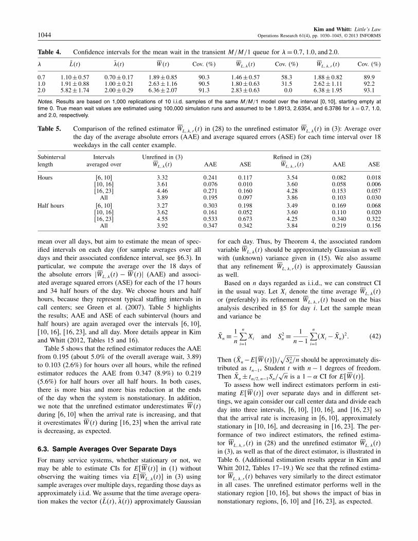
Table 4. Confidence intervals for the mean wait in the transient M/M/1 queue for �= 00711001 and 200.
� L4t5 �4t5 SW4t5 Cov. 4%5 SWL1�4t5 Cov. 4%5 SWL1�1 r4t5 Cov. 4%5
0.7 1010 ± 0057 0070 ± 0017 1089 ± 0085 9003 1046 ± 0057 5803 1088 ± 0082 89091.0 1091 ± 0088 1000 ± 0021 2063 ± 1016 9005 1080 ± 0063 3105 2062 ± 1011 92022.0 5082 ± 1074 2000 ± 0029 6036 ± 2007 9103 2083 ± 0063 000 6038 ± 1095 9301
Notes. Results are based on 1,000 replications of 10 i.i.d. samples of the same M/M/1 model over the interval [0110], starting empty attime 0. True mean wait values are estimated using 100,000 simulation runs and assumed to be 1.8913, 2.6354, and 6.3786 for �= 007, 1.0,and 2.0, respectively.
Table 5. Comparison of the refined estimator SWL1�1 r4t5 in (28) to the unrefined estimator SWL1�4t5 in (3): Average overthe day of the average absolute errors (AAE) and average squared errors (ASE) for each time interval over 18weekdays in the call center example.
Subinterval Intervals Unrefined in (3) Refined in (28)length averaged over SWL1�4t5 AAE ASE SWL1�1 r4t5 AAE ASE
Hours [6110] 3032 00241 00117 3054 00082 00018[10116] 3061 00076 00010 3060 00058 00006[16123] 4046 00271 00160 4028 00153 00057
All 3089 00195 00097 3086 00103 00030Half hours [6110] 3027 00303 00198 3049 00169 00068
[10116] 3062 00161 00052 3060 00110 00020[16123] 4055 00533 00673 4025 00340 00322
All 3092 00347 00342 3084 00219 00156
mean over all days, but aim to estimate the mean of spec-ified intervals on each day (for sample averages over alldays and their associated confidence interval, see §6.3). Inparticular, we compute the average over the 18 days ofthe absolute errors �SWL1�4t5 − SW4t5� (AAE) and associ-ated average squared errors (ASE) for each of the 17 hoursand 34 half hours of the day. We choose hours and halfhours, because they represent typical staffing intervals incall centers; see Green et al. (2007). Table 5 highlightsthe results; AAE and ASE of each subinterval (hours andhalf hours) are again averaged over the intervals 661107,6101167, 6161237, and all day. More details appear in Kimand Whitt (2012, Tables 15 and 16).
Table 5 shows that the refined estimator reduces the AAEfrom 00195 (about 500% of the overall average wait, 3089)to 00103 (2.6%) for hours over all hours, while the refinedestimator reduces the AAE from 00347 (809%) to 00219(5.6%) for half hours over all half hours. In both cases,there is more bias and more bias reduction at the endsof the day when the system is nonstationary. In addition,we note that the unrefined estimator underestimates SW4t5during [6110] when the arrival rate is increasing, and thatit overestimates SW4t5 during [16123] when the arrival rateis decreasing, as expected.
6.3. Sample Averages Over Separate Days
For many service systems, whether stationary or not, wemay be able to estimate CIs for E6SW4t57 in (1) withoutobserving the waiting times via E6SWL1�4t57 in (3) usingsample averages over multiple days, regarding those days asapproximately i.i.d. We assume that the time average opera-tion makes the vector 4L4t51 �4t55 approximately Gaussian
for each day. Thus, by Theorem 4, the associated randomvariable SWL1�4t5 should be approximately Gaussian as wellwith (unknown) variance given in (15). We also assumethat any refinement SWL1�1 r4t5 is approximately Gaussianas well.
Based on n days regarded as i.i.d., we can construct CIin the usual way. Let Xi denote the time average SWL1�4t5or (preferably) its refinement SWL1�1 r4t5 based on the biasanalysis described in §5 for day i. Let the sample meanand variance be
Xn ≡1n
n∑
i=1
Xi and S2n ≡
1n− 1
n∑
i=1
4Xi − Xn520 (42)
Then 4Xn−E6SW4t575/√
S2n/n should be approximately dis-
tributed as tn−1, Student t with n− 1 degrees of freedom.Then Xn ± t�/21 n−1Sn/
√n is a 1 −� CI for E6SW4t57.
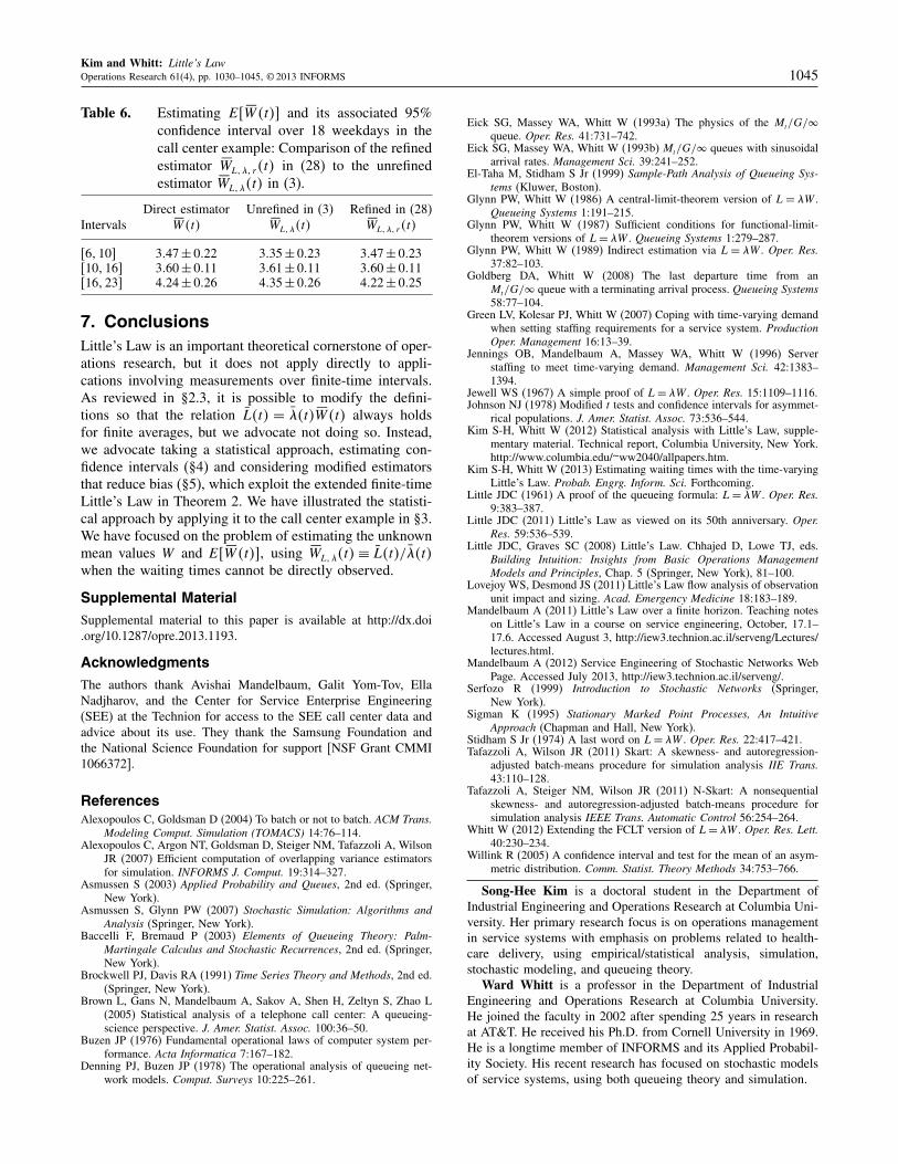
To assess how well indirect estimators perform in esti-mating E6SW4t57 over separate days and in different set-tings, we again consider our call center data and divide eachday into three intervals, [6110], [10116], and [16123] sothat the arrival rate is increasing in [6110], approximatelystationary in [10116], and decreasing in [16123]. The per-formance of two indirect estimators, the refined estima-tor SWL1�1 r4t5 in (28) and the unrefined estimator SWL1�4t5in (3), as well as that of the direct estimator, is illustrated inTable 6. (Additional estimation results appear in Kim andWhitt 2012, Tables 17–19.) We see that the refined estima-tor SWL1�1 r4t5 behaves very similarly to the direct estimatorin all cases. The unrefined estimator performs well in thestationary region [10116], but shows the impact of bias innonstationary regions, [6110] and [16123], as expected.
Kim and Whitt: Little’s LawOperations Research 61(4), pp. 1030–1045, © 2013 INFORMS 1045
Table 6. Estimating E6SW4t57 and its associated 95%confidence interval over 18 weekdays in thecall center example: Comparison of the refinedestimator SWL1�1 r4t5 in (28) to the unrefinedestimator SWL1�4t5 in (3).
Direct estimator Unrefined in (3) Refined in (28)Intervals SW4t5 SWL1�4t5 SWL1�1 r4t5
661107 3047 ± 0022 3035 ± 0023 3047 ± 00236101167 3060 ± 0011 3061 ± 0011 3060 ± 00116161237 4024 ± 0026 4035 ± 0026 4022 ± 0025
7. ConclusionsLittle’s Law is an important theoretical cornerstone of oper-ations research, but it does not apply directly to appli-cations involving measurements over finite-time intervals.As reviewed in §2.3, it is possible to modify the defini-tions so that the relation L4t5 = �4t5SW4t5 always holdsfor finite averages, but we advocate not doing so. Instead,we advocate taking a statistical approach, estimating con-fidence intervals (§4) and considering modified estimatorsthat reduce bias (§5), which exploit the extended finite-timeLittle’s Law in Theorem 2. We have illustrated the statisti-cal approach by applying it to the call center example in §3.We have focused on the problem of estimating the unknownmean values W and E6SW4t571 using SWL1�4t5 ≡ L4t5/�4t5when the waiting times cannot be directly observed.
Supplemental MaterialSupplemental material to this paper is available at http://dx.doi.org/10.1287/opre.2013.1193.
AcknowledgmentsThe authors thank Avishai Mandelbaum, Galit Yom-Tov, EllaNadjharov, and the Center for Service Enterprise Engineering(SEE) at the Technion for access to the SEE call center data andadvice about its use. They thank the Samsung Foundation andthe National Science Foundation for support [NSF Grant CMMI1066372].
ReferencesAlexopoulos C, Goldsman D (2004) To batch or not to batch. ACM Trans.
Modeling Comput. Simulation (TOMACS) 14:76–114.Alexopoulos C, Argon NT, Goldsman D, Steiger NM, Tafazzoli A, Wilson
JR (2007) Efficient computation of overlapping variance estimatorsfor simulation. INFORMS J. Comput. 19:314–327.
Asmussen S (2003) Applied Probability and Queues, 2nd ed. (Springer,New York).
Asmussen S, Glynn PW (2007) Stochastic Simulation: Algorithms andAnalysis (Springer, New York).
Baccelli F, Bremaud P (2003) Elements of Queueing Theory: Palm-Martingale Calculus and Stochastic Recurrences, 2nd ed. (Springer,New York).
Brockwell PJ, Davis RA (1991) Time Series Theory and Methods, 2nd ed.(Springer, New York).
Brown L, Gans N, Mandelbaum A, Sakov A, Shen H, Zeltyn S, Zhao L(2005) Statistical analysis of a telephone call center: A queueing-science perspective. J. Amer. Statist. Assoc. 100:36–50.
Buzen JP (1976) Fundamental operational laws of computer system per-formance. Acta Informatica 7:167–182.
Denning PJ, Buzen JP (1978) The operational analysis of queueing net-work models. Comput. Surveys 10:225–261.
Eick SG, Massey WA, Whitt W (1993a) The physics of the Mt/G/�queue. Oper. Res. 41:731–742.
Eick SG, Massey WA, Whitt W (1993b) Mt/G/� queues with sinusoidalarrival rates. Management Sci. 39:241–252.
El-Taha M, Stidham S Jr (1999) Sample-Path Analysis of Queueing Sys-tems (Kluwer, Boston).
Glynn PW, Whitt W (1986) A central-limit-theorem version of L = �W .Queueing Systems 1:191–215.
Glynn PW, Whitt W (1987) Sufficient conditions for functional-limit-theorem versions of L= �W . Queueing Systems 1:279–287.
Glynn PW, Whitt W (1989) Indirect estimation via L = �W . Oper. Res.37:82–103.
Goldberg DA, Whitt W (2008) The last departure time from anMt/G/� queue with a terminating arrival process. Queueing Systems58:77–104.
Green LV, Kolesar PJ, Whitt W (2007) Coping with time-varying demandwhen setting staffing requirements for a service system. ProductionOper. Management 16:13–39.
Jennings OB, Mandelbaum A, Massey WA, Whitt W (1996) Serverstaffing to meet time-varying demand. Management Sci. 42:1383–1394.
Jewell WS (1967) A simple proof of L= �W . Oper. Res. 15:1109–1116.Johnson NJ (1978) Modified t tests and confidence intervals for asymmet-
rical populations. J. Amer. Statist. Assoc. 73:536–544.Kim S-H, Whitt W (2012) Statistical analysis with Little’s Law, supple-
mentary material. Technical report, Columbia University, New York.http://www.columbia.edu/~ww2040/allpapers.htm.
Kim S-H, Whitt W (2013) Estimating waiting times with the time-varyingLittle’s Law. Probab. Engrg. Inform. Sci. Forthcoming.
Little JDC (1961) A proof of the queueing formula: L= �W . Oper. Res.9:383–387.
Little JDC (2011) Little’s Law as viewed on its 50th anniversary. Oper.Res. 59:536–539.
Little JDC, Graves SC (2008) Little’s Law. Chhajed D, Lowe TJ, eds.Building Intuition: Insights from Basic Operations ManagementModels and Principles, Chap. 5 (Springer, New York), 81–100.
Lovejoy WS, Desmond JS (2011) Little’s Law flow analysis of observationunit impact and sizing. Acad. Emergency Medicine 18:183–189.
Mandelbaum A (2011) Little’s Law over a finite horizon. Teaching noteson Little’s Law in a course on service engineering, October, 17.1–17.6. Accessed August 3, http://iew3.technion.ac.il/serveng/Lectures/lectures.html.
Mandelbaum A (2012) Service Engineering of Stochastic Networks WebPage. Accessed July 2013, http://iew3.technion.ac.il/serveng/.
Serfozo R (1999) Introduction to Stochastic Networks (Springer,New York).
Sigman K (1995) Stationary Marked Point Processes, An IntuitiveApproach (Chapman and Hall, New York).
Stidham S Jr (1974) A last word on L= �W . Oper. Res. 22:417–421.Tafazzoli A, Wilson JR (2011) Skart: A skewness- and autoregression-
adjusted batch-means procedure for simulation analysis IIE Trans.43:110–128.
Tafazzoli A, Steiger NM, Wilson JR (2011) N-Skart: A nonsequentialskewness- and autoregression-adjusted batch-means procedure forsimulation analysis IEEE Trans. Automatic Control 56:254–264.
Whitt W (2012) Extending the FCLT version of L= �W . Oper. Res. Lett.40:230–234.
Willink R (2005) A confidence interval and test for the mean of an asym-metric distribution. Comm. Statist. Theory Methods 34:753–766.
Song-Hee Kim is a doctoral student in the Department ofIndustrial Engineering and Operations Research at Columbia Uni-versity. Her primary research focus is on operations managementin service systems with emphasis on problems related to health-care delivery, using empirical/statistical analysis, simulation,stochastic modeling, and queueing theory.
Ward Whitt is a professor in the Department of IndustrialEngineering and Operations Research at Columbia University.He joined the faculty in 2002 after spending 25 years in researchat AT&T. He received his Ph.D. from Cornell University in 1969.He is a longtime member of INFORMS and its Applied Probabil-ity Society. His recent research has focused on stochastic modelsof service systems, using both queueing theory and simulation.