Babusiaux, C, van Leeuwen, F, Barstow, MA, Jordi, C, Vallenari, A, Bossini, D,

Bressan, A, Cantat-Gaudin, T, van Leeuwen, M, Brown, AGA, Prusti, T, de

Bruijne, JHJ, Bailer-Jones, CAL, Biermann, M, Evans, DW, Eyer, L, Jansen, F,

Klioner, SA, Lammers, U, Lindegren, L, Luri, X, Mignard, F, Panem, C,

Pourbaix, D, Randich, S, Sartoretti, P, Siddiqui, HI, Soubiran, C, Walton, NA,

Arenou, F, Bastian, U, Cropper, M, Drimmel, R, Katz, D, Lattanzi, MG, Bakker, J,

Cacciari, C, Castaneda, J, Chaoul, L, Cheek, N, De Angeli, F, Fabricius, C,

Guerra, R, Holl, B, Masana, E, Messineo, R, Mowlavi, N, Nienartowicz, K,

Panuzzo, P, Portell, J, Riello, M, Seabroke, GM, Tanga, P, Thevenin, F, Gracia-

Abril, G, Comoretto, G, Garcia-Reinaldos, M, Teyssier, D, Altmann, M, Andrae,

R, Audard, M, Bellas-Velidis, I, Benson, K, Berthier, J, Blomme, R, Burgess, P,

Busso, G, Carry, B, Cellino, A, Clementini, G, Clotet, M, Creevey, O, Davidson,

M, De Ridder, J, Delchambre, L, Dell'Oro, A, Ducourant, C, Fernandez-

Hernandez, J, Fouesneau, M, Fremat, Y, Galluccio, L, Garcia-Torres, M,

Gonzalez-Nunez, J, Gonzalez-Vidal, JJ, Gosset, E, Guy, LP, Halbwachs, J-L,

Hambly, NC, Harrison, DL, Hernandez, J, Hestroffer, D, Hodgkin, ST, Hutton, A,

Jasniewicz, G, Jean-Antoine-Piccolo, A, Jordan, S, Korn, AJ, Krone-Martins, A,

Lanzafame, AC, Lebzelter, T, Loeffler, W, Manteiga, M, Marrese, PM, Martin-

Fleitas, JM, Moitinho, A, Mora, A, Muinonen, K, Osinde, J, Pancino, E, Pauwels,

T, Petit, J-M, Recio-Blanco, A, Richards, PJ, Rimoldini, L, Robin, AC, Sarro, LM,

Siopis, C, Smith, M, Sozzetti, A, Sueveges, M, Torra, J, van Reeven, W, Abbas,

U, Abreu Aramburu, A, Accart, S, Aerts, C, Altavilla, G, Alvarez, MA, Alvarez, R,

Alves, J, Anderson, RI, Andrei, AH, Anglada Varela, E, Antiche, E, Antoja, T,

Arcay, B, Astraatmadja, TL, Bach, N, Baker, SG, Balaguer-Nunez, L, Balm, P,

Barache, C, Barata, C, Barbato, D, Barblan, F, Barklem, PS, Barrado, D, Barros,

M, Bartholome Munoz, S, Bassilana, J-L, Becciani, U, Bellazzini, M, Berihuete,

A, Bertones, S, Bianchi, L, Bienayme, O, Blanco-Cuaresma, S, Boch, T,

Boeche, C, Bombrun, A, Borrachero, R, Bouquillon, S, Bourda, G, Bragaglia, A,

Bramante, L, Breddels, MA, Brouillet, N, Bruesemeister, T, Brugaletta, E,

Bucciarelli, B, Burlacu, A, Busonero, D, Butkevich, AG, Buzzi, R, Caffau, E,

Cancelliere, R, Cannizzaro, G, Carballo, R, Carlucci, T, Carrasco, JM,

Casamiquela, L, Castellani, M, Castro-Ginard, A, Charlot, P, Chemin, L,

Chiavassa, A, Cocozza, G, Costigan, G, Cowell, S, Crifo, F, Crosta, M, Crowley,

C, Cuypers, J, Dafonte, C, Damerdji, Y, Dapergolas, A, David, P, David, M, de

http://researchonline.ljmu.ac.uk/

LJMU Research Online

laverny, P, De Luise, F, De March, R, de Martino, D, de Souza, R, de Torres, A,

Debosscher, J, del Pozo, E, Delbo, M, Delgado, A, Delgado, HE, Diakite, S,

Diener, C, Distefano, E, Dolding, C, Drazinos, P, Duran, J, Edvardsson, B,

Enke, H, Eriksson, K, Esquej, P, Bontemps, GE, Fabre, C, Fabrizio, M, Faigler,

S, Falcao, AJ, Casas, MF, Federici, L, Fedorets, G, Fernique, P, Figueras, F,

Filippi, F, Findeisen, K, Fonti, A, Fraile, E, Fraser, M, Frezouls, B, Gai, M,

Galleti, S, Garabato, D, Garcia-Sedano, F, Garofalo, A, Garralda, N, Gavel, A,

Gavras, P, Gerssen, J, Geyer, R, Giacobbe, P, Gilmore, G, Girona, S, Giuffrida,

G, Glass, F, Gomes, M, Granvik, M, Gueguen, A, Guerrier, A, Guiraud, J,

Gutierrez-Sanchez, R, Haigron, R, Hatzidimitriou, D, Hauser, M, Haywood, M,

Heiter, U, Helmi, A, Heu, J, Hilger, T, Hobbs, D, Hofmann, W, Holland, G,

Huckle, HE, Hypki, A, Icardi, V, Janssen, K, Jevardat de Fombelle, G, Jonker,

PG, Juhasz, AL, Julbe, F, Karampelas, A, Kewley, A, Klar, J, Kochoska, A,

Kohley, R, Kolenberg, K, Kontizas, M, Kontizas, E, Koposov, SE, Kordopatis,

G, Kostrzewa-Rutkowska, Z, Koubsky, P, Lambert, S, Lanza, AF, Lasne, Y,

Lavigne, J-B, Le Fustec, Y, Le Poncin-Lafitte, C, Lebreton, Y, Leccia, S,

Leclerc, N, Lecoeur-Taibi, I, Lenhardt, H, Leroux, F, Liao, S, Licata, E,

Lindstrom, HEP, Lister, TA, Livanou, E, Lobel, A, Lopez, M, Managau, S, Mann,

RG, Mantelet, G, Marchal, O, Marchant, JM, Marconi, M, Marinoni, S,

Marschalko, G, Marshall, DJ, Martino, M, Marton, G, Mary, N, Massari, D,

Matijevic, G, Mazeh, T, McMillan, PJ, Messina, S, Michalik, D, Millar, NR, Molina,

D, Molinaro, R, Molnar, L, Montegriffo, P, Mor, R, Morbidelli, R, Morel, T, Morris,

D, Mulone, AF, Muraveva, T, Musella, I, Nelemans, G, Nicastro, L, Noval, L,

O'Mullane, W, Ordenovic, C, Ordonez-Blanco, D, Osborne, P, Pagani, C,

Pagano, I, Pailler, F, Palacin, H, Palaversa, L, Panahi, A, Pawlak, M, Piersimoni,

AM, Pineau, F-X, Plachy, E, Plum, G, Poggio, E, Poujoulet, E, Prsa, A, Pulone,

L, Racero, E, Ragaini, S, Rambaux, N, Ramos-Lerate, M, Regibo, S, Reyle, C,

Riclet, F, Ripepi, V, Riva, A, Rivard, A, Rixon, G, Roegiers, T, Roelens, M,

Romero-Gomez, M, Rowell, N, Royer, F, Ruiz-Dern, L, Sadowski, G, Sagrista

Selles, T, Sahlmann, J, Salgado, J, Salguero, E, Sanna, N, Santana-Ros, T,

Sarasso, M, Savietto, H, Schultheis, M, Sciacca, E, Segol, M, Segovia, JC,

Segransan, D, Shih, I-C, Siltala, L, Silva, AF, Smart, RL, Smith, KW, Solano, E,

Solitro, F, Sordo, R, Soria Nieto, S, Souchay, J, Spagna, A, Spoto, F, Stampa,

U, Steele, IA, Steidelmueller, H, Stephenson, CA, Stoev, H, Suess, FF, Surdej,

J, Szabados, L, Szegedi-Elek, E, Tapiador, D, Taris, F, Tauran, G, Taylor, MB,

Teixeira, R, Terrett, D, Teyssandier, P, Thuillot, W, Titarenko, A, Clotet, FT,

Turon, C, Ulla, A, Utrilla, E, Uzzi, S, Vaillant, M, Valentini, G, Valette, V, van

Elteren, A, Van Hemelryck, E, Vaschetto, M, Vecchiato, A, Veljanoski, J, Viala,

Y, Vicente, D, Vogt, S, von Essen, C, Voss, H, Votruba, V, Voutsinas, S,

Walmsley, G, Weiler, M, Wertz, O, Wevers, T, Wyrzykowski, L, Yoldas, A, Zerjal,

M, Ziaeepour, H, Zorec, J, Zschocke, S, Zucker, S, Zurbach, C and Zwitter, T

Gaia Data Release 2 Observational Hertzsprung-Russell diagrams

http://researchonline.ljmu.ac.uk/

http://researchonline.ljmu.ac.uk/9650/

Article

LJMU has developed LJMU Research Online for users to access the research output of the

University more effectively. Copyright © and Moral Rights for the papers on this site are retained by

the individual authors and/or other copyright owners. Users may download and/or print one copy of

any article(s) in LJMU Research Online to facilitate their private study or for non-commercial research.

You may not engage in further distribution of the material or use it for any profit-making activities or

any commercial gain.

The version presented here may differ from the published version or from the version of the record.

Please see the repository URL above for details on accessing the published version and note that

access may require a subscription.

For more information please contact researchonline@ljmu.ac.uk

http://researchonline.ljmu.ac.uk/

Citation (please note it is advisable to refer to the publisher’s version if you

intend to cite from this work)

Babusiaux, C, van Leeuwen, F, Barstow, MA, Jordi, C, Vallenari, A, Bossini,

D, Bressan, A, Cantat-Gaudin, T, van Leeuwen, M, Brown, AGA, Prusti, T, de

Bruijne, JHJ, Bailer-Jones, CAL, Biermann, M, Evans, DW, Eyer, L, Jansen,

F, Klioner, SA, Lammers, U, Lindegren, L, Luri, X, Mignard, F, Panem, C,

Astronomy&

Astrophysics

Special issue

A&A 616, A10 (2018)https://doi.org/10.1051/0004-6361/201832843© ESO 2018

Gaia Data Release 2

Gaia Data Release 2

Observational Hertzsprung-Russell diagrams⋆

Gaia Collaboration, C. Babusiaux1, 2,⋆⋆ , F. van Leeuwen3, M. A. Barstow4, C. Jordi5, A. Vallenari6, D. Bossini6,A. Bressan7, T. Cantat-Gaudin6, 5, M. van Leeuwen3, A. G. A. Brown8, T. Prusti9, J. H. J. de Bruijne9,

C. A. L. Bailer-Jones10, M. Biermann11, D. W. Evans3, L. Eyer12, F. Jansen13, S. A. Klioner14, U. Lammers15,L. Lindegren16, X. Luri5, F. Mignard17, C. Panem18, D. Pourbaix19, 20, S. Randich21, P. Sartoretti2, H. I. Siddiqui22,C. Soubiran23, N. A. Walton3, F. Arenou2, U. Bastian11, M. Cropper24, R. Drimmel25, D. Katz2, M. G. Lattanzi25,

J. Bakker15, C. Cacciari26, J. Castañeda5, L. Chaoul18, N. Cheek27, F. De Angeli3, C. Fabricius5, R. Guerra15,B. Holl12, E. Masana5, R. Messineo28, N. Mowlavi12, K. Nienartowicz29, P. Panuzzo2, J. Portell5, M. Riello3,

G. M. Seabroke24, P. Tanga17, F. Thévenin17, G. Gracia-Abril30, 11, G. Comoretto22, M. Garcia-Reinaldos15,D. Teyssier22, M. Altmann11, 31, R. Andrae10, M. Audard12, I. Bellas-Velidis32, K. Benson24, J. Berthier33,

R. Blomme34, P. Burgess3, G. Busso3, B. Carry17, 33, A. Cellino25, G. Clementini26, M. Clotet5, O. Creevey17,M. Davidson35, J. De Ridder36, L. Delchambre37, A. Dell’Oro21, C. Ducourant23, J. Fernández-Hernández38,

M. Fouesneau10, Y. Frémat34, L. Galluccio17, M. García-Torres39, J. González-Núñez27, 40, J. J. González-Vidal5,E. Gosset37, 20, L. P. Guy29, 41, J.-L. Halbwachs42, N. C. Hambly35, D. L. Harrison3, 43, J. Hernández15,D. Hestroffer33, S. T. Hodgkin3, A. Hutton44, G. Jasniewicz45, A. Jean-Antoine-Piccolo18, S. Jordan11,

A. J. Korn46, A. Krone-Martins47, A. C. Lanzafame48, 49, T. Lebzelter50, W. Löffler11, M. Manteiga51, 52,P. M. Marrese53, 54, J. M. Martín-Fleitas44, A. Moitinho47, A. Mora44, K. Muinonen55, 56, J. Osinde57,

E. Pancino21, 54, T. Pauwels34, J.-M. Petit58, A. Recio-Blanco17, P. J. Richards59, L. Rimoldini29, A. C. Robin58,L. M. Sarro60, C. Siopis19, M. Smith24, A. Sozzetti25, M. Süveges10, J. Torra5, W. van Reeven44, U. Abbas25,

A. Abreu Aramburu61, S. Accart62, C. Aerts36, 63, G. Altavilla53, 54, 26, M. A. Álvarez51, R. Alvarez15, J. Alves50,R. I. Anderson64, 12, A. H. Andrei65, 66, 31, E. Anglada Varela38, E. Antiche5, T. Antoja9, 5, B. Arcay51,

T. L. Astraatmadja10, 67, N. Bach44, S. G. Baker24, L. Balaguer-Núñez5, P. Balm22, C. Barache31, C. Barata47,D. Barbato68, 25, F. Barblan12, P. S. Barklem46, D. Barrado69, M. Barros47, S. Bartholomé Muñoz5,

J.-L. Bassilana62, U. Becciani49, M. Bellazzini26, A. Berihuete70, S. Bertone25, 31, 71, L. Bianchi72, O. Bienaymé42,S. Blanco-Cuaresma12, 23, 73, T. Boch42, C. Boeche6, A. Bombrun74, R. Borrachero5, S. Bouquillon31, G. Bourda23,

A. Bragaglia26, L. Bramante28, M. A. Breddels75, N. Brouillet23, T. Brüsemeister11, E. Brugaletta49,B. Bucciarelli25, A. Burlacu18, D. Busonero25, A. G. Butkevich14, R. Buzzi25, E. Caffau2, R. Cancelliere76,

G. Cannizzaro77, 63, R. Carballo78, T. Carlucci31, J. M. Carrasco5, L. Casamiquela5, M. Castellani53,A. Castro-Ginard5, P. Charlot23, L. Chemin79, A. Chiavassa17, G. Cocozza26, G. Costigan8, S. Cowell3, F. Crifo2,

M. Crosta25, C. Crowley74, J. Cuypers†34, C. Dafonte51, Y. Damerdji37, 80, A. Dapergolas32, P. David33,M. David81, P. de Laverny17, F. De Luise82, R. De March28, D. de Martino83, R. de Souza84, A. de Torres74,

J. Debosscher36, E. del Pozo44, M. Delbo17, A. Delgado3, H. E. Delgado60, S. Diakite58, C. Diener3,E. Distefano49, C. Dolding24, P. Drazinos85, J. Durán57, B. Edvardsson46, H. Enke86, K. Eriksson46, P. Esquej87,G. Eynard Bontemps18, C. Fabre88, M. Fabrizio53, 54, S. Faigler89, A. J. Falcão90, M. Farràs Casas5, L. Federici26,

G. Fedorets55, P. Fernique42, F. Figueras5, F. Filippi28, K. Findeisen2, A. Fonti28, E. Fraile87, M. Fraser3, 91,B. Frézouls18, M. Gai25, S. Galleti26, D. Garabato51, F. García-Sedano60, A. Garofalo92, 26, N. Garralda5,

A. Gavel46, P. Gavras2, 32, 85, J. Gerssen86, R. Geyer14, P. Giacobbe25, G. Gilmore3, S. Girona93, G. Giuffrida54, 53,F. Glass12, M. Gomes47, M. Granvik55, 94, A. Gueguen2, 95, A. Guerrier62, J. Guiraud18, R. Gutiérrez-Sánchez22,

R. Haigron2, D. Hatzidimitriou85, 32, M. Hauser11, 10, M. Haywood2, U. Heiter46, A. Helmi75, J. Heu2, T. Hilger14,D. Hobbs16, W. Hofmann11, G. Holland3, H. E. Huckle24, A. Hypki8, 96, V. Icardi28, K. Janßen86,

G. Jevardat de Fombelle29, P. G. Jonker77, 63, Á. L. Juhász97, 98, F. Julbe5, A. Karampelas85, 99, A. Kewley3,

⋆ The full Table A.1 is only available at the CDS via anonymous ftp to cdsarc.u-strasbg.fr (130.79.128.5) or viahttp://cdsarc.u-strasbg.fr/viz-bin/qcat?J/A+A/616/A10⋆⋆ Corresponding author: C. Babusiaux, e-mail: carine.babusiaux@univ-grenoble-alpes.fr

A10, page 1 of 29

Open Access article, published by EDP Sciences, under the terms of the Creative Commons Attribution License (http://creativecommons.org/licenses/by/4.0),which permits unrestricted use, distribution, and reproduction in any medium, provided the original work is properly cited.

A&A 616, A10 (2018)

J. Klar86, A. Kochoska100, 101, R. Kohley15, K. Kolenberg73, 102, 36, M. Kontizas85, E. Kontizas32, S. E. Koposov3, 103,G. Kordopatis17, Z. Kostrzewa-Rutkowska77, 63, P. Koubsky104, S. Lambert31, A. F. Lanza49, Y. Lasne62,

J.-B. Lavigne62, Y. Le Fustec105, C. Le Poncin-Lafitte31, Y. Lebreton2, 106, S. Leccia83, N. Leclerc2,I. Lecoeur-Taibi29, H. Lenhardt11, F. Leroux62, S. Liao25, 107, 108, E. Licata72, H. E. P. Lindstrøm109, 110,

T. A. Lister111, E. Livanou85, A. Lobel34, M. López69, S. Managau62, R. G. Mann35, G. Mantelet11, O. Marchal2,J. M. Marchant112, M. Marconi83, S. Marinoni53, 54, G. Marschalkó97, 113, D. J. Marshall114, M. Martino28,

G. Marton97, N. Mary62, D. Massari75, G. Matijevic86, T. Mazeh89, P. J. McMillan16, S. Messina49, D. Michalik16,N. R. Millar3, D. Molina5, R. Molinaro83, L. Molnár97, P. Montegriffo26, R. Mor5, R. Morbidelli25, T. Morel37,

D. Morris35, A. F. Mulone28, T. Muraveva26, I. Musella83, G. Nelemans63, 36, L. Nicastro26, L. Noval62,W. O’Mullane15, 41, C. Ordénovic17, D. Ordóñez-Blanco 29, P. Osborne3, C. Pagani4, I. Pagano49, F. Pailler18,H. Palacin62, L. Palaversa3, 12, A. Panahi89, M. Pawlak115, 116, A. M. Piersimoni82, F.-X. Pineau42, E. Plachy97,G. Plum2, E. Poggio68, 25, E. Poujoulet117, A. Prša101, L. Pulone53, E. Racero27, S. Ragaini26, N. Rambaux33,

M. Ramos-Lerate118, S. Regibo36, C. Reylé58, F. Riclet18, V. Ripepi83, A. Riva25, A. Rivard62, G. Rixon3,T. Roegiers119, M. Roelens12, M. Romero-Gómez5, N. Rowell35, F. Royer2, L. Ruiz-Dern2, G. Sadowski19,

T. Sagristà Sellés11, J. Sahlmann15, 120, J. Salgado121, E. Salguero38, N. Sanna21, T. Santana-Ros96, M. Sarasso25,H. Savietto122, M. Schultheis17, E. Sciacca49, M. Segol123, J. C. Segovia27, D. Ségransan12, I-C. Shih2,

L. Siltala55, 124, A. F. Silva47, R. L. Smart25, K. W. Smith10, E. Solano69, 125, F. Solitro28, R. Sordo6,S. Soria Nieto5, J. Souchay31, A. Spagna25, F. Spoto17, 33, U. Stampa11, I. A. Steele112, H. Steidelmüller14,

C. A. Stephenson22, H. Stoev126, F. F. Suess3, J. Surdej37, L. Szabados97, E. Szegedi-Elek97, D. Tapiador127, 128,F. Taris31, G. Tauran62, M. B. Taylor129, R. Teixeira84, D. Terrett59, P. Teyssandier31, W. Thuillot33, A. Titarenko17,

F. Torra Clotet130, C. Turon2, A. Ulla131, E. Utrilla44, S. Uzzi28, M. Vaillant62, G. Valentini82, V. Valette18,A. van Elteren8, E. Van Hemelryck34, M. Vaschetto28, A. Vecchiato25, J. Veljanoski75, Y. Viala2, D. Vicente93,S. Vogt119, C. von Essen132, H. Voss5, V. Votruba104, S. Voutsinas35, G. Walmsley18, M. Weiler5, O. Wertz133,T. Wevers3, 63, Ł. Wyrzykowski3, 115, A. Yoldas3, M. Žerjal100, 134, H. Ziaeepour58, J. Zorec135, S. Zschocke14,

S. Zucker136, C. Zurbach45, and T. Zwitter100

(Affiliations can be found after the references)

Received 16 February 2018 / Accepted 16 April 2018

ABSTRACT

Context. Gaia Data Release 2 provides high-precision astrometry and three-band photometry for about 1.3 billion sources over thefull sky. The precision, accuracy, and homogeneity of both astrometry and photometry are unprecedented.Aims. We highlight the power of the Gaia DR2 in studying many fine structures of the Hertzsprung-Russell diagram (HRD). Gaiaallows us to present many different HRDs, depending in particular on stellar population selections. We do not aim here for completenessin terms of types of stars or stellar evolutionary aspects. Instead, we have chosen several illustrative examples.Methods. We describe some of the selections that can be made in Gaia DR2 to highlight the main structures of the Gaia HRDs.We select both field and cluster (open and globular) stars, compare the observations with previous classifications and with stellarevolutionary tracks, and we present variations of the Gaia HRD with age, metallicity, and kinematics. Late stages of stellar evolutionsuch as hot subdwarfs, post-AGB stars, planetary nebulae, and white dwarfs are also analysed, as well as low-mass brown dwarf objects.Results. The Gaia HRDs are unprecedented in both precision and coverage of the various Milky Way stellar populations and stellarevolutionary phases. Many fine structures of the HRDs are presented. The clear split of the white dwarf sequence into hydrogen andhelium white dwarfs is presented for the first time in an HRD. The relation between kinematics and the HRD is nicely illustrated.Two different populations in a classical kinematic selection of the halo are unambiguously identified in the HRD. Membership andmean parameters for a selected list of open clusters are provided. They allow drawing very detailed cluster sequences, highlighting finestructures, and providing extremely precise empirical isochrones that will lead to more insight in stellar physics.Conclusions. Gaia DR2 demonstrates the potential of combining precise astrometry and photometry for large samples for studies instellar evolution and stellar population and opens an entire new area for HRD-based studies.

Key words. parallaxes – Hertzsprung-Russell and C-M diagrams – solar neighborhood – stars: evolution

1. Introduction

The Hertzsprung-Russell diagram (HRD) is one of the mostimportant tools in stellar studies. It illustrates empirically therelationship between stellar spectral type (or temperature orcolour index) and luminosity (or absolute magnitude). Theposition of a star in the HRD is mainly given by its initial mass,chemical composition, and age, but effects such as rotation,

stellar wind, magnetic field, detailed chemical abundance, over-shooting, and non-local thermal equilibrium also play a role.Therefore, the detailed HRD features are important to constrainstellar structure and evolutionary studies as well as stellar atmo-sphere modelling. Up to now, a proper understanding of thephysical process in the stellar interior and the exact contributionof each of the effects mentioned are missing because we lacklarge precise and homogeneous samples that cover the full

A10, page 2 of 29

Gaia Collaboration (Babusiaux, C. et al.): Gaia Data Release 2

HRD. Moreover, a precise HRD provides a great framework forexploring stellar populations and stellar systems.

Up to now, the most complete solar neighbourhood empiri-cal HRD could be obtained by combining the HIPPARCOS data(Perryman et al. 1995) with nearby stellar catalogues to providethe faint end (e.g. Gliese & Jahreiß 1991; Henry & Jao 2015).Clusters provide empirical HRDs for a range of ages and metalcontents and are therefore widely used in stellar evolution stud-ies. To be conclusive, they need homogeneous photometry forinter-comparisons and astrometry for good memberships.

With its global census of the whole sky, homogeneousastrometry, and photometry of unprecedented accuracy, GaiaDR2 is setting a new major step in stellar, galactic, and extra-galactic studies. It provides position, trigonometric parallax, andproper motion as well as three broad-band magnitudes (G, GBP,and GRP) for more than a billion objects brighter than G ∼ 20,plus radial velocity for sources brighter than GRVS ∼ 12 mag andphotometry for variable stars (Gaia Collaboration 2018a). Theamount, exquisite quality, and homogeneity of the data allowsreaching a level of detail in the HRDs that has never been reachedbefore. The number of open clusters with accurate parallax infor-mation is unprecedented, and new open clusters or associationswill be discovered. Gaia DR2 provides absolute parallax forfaint red dwarfs and the faintest white dwarfs for the first time.

This paper is one of the papers accompanying the GaiaDR2 release. The following papers describe the data used here:Gaia Collaboration (2018a) for an overview, Lindegren et al.(2018) for the astrometry, Evans et al. (2018) for the photometry,and Arenou et al. (2018) for the global validation. Someone inter-ested in this HRD paper may also be interested in the variabilityin the HRD described in Gaia Collaboration (2018b), in the firstattempt to derive an HRD using temperatures and luminositiesfrom the Gaia DR2 data of Andrae et al. (2018), in the kinematicsof the globular clusters discussed in Gaia Collaboration (2018c),and in the field kinematics presented in Gaia Collaboration(2018d).

In this paper, Sect. 2 presents a global description of how webuilt the Gaia HRDs of both field and cluster stars, the filtersthat we applied, and the handling of the extinction. In Sect. 3 wepresent our selection of cluster data; the handling of the globularclusters is detailed in Gaia Collaboration (2018c) and the han-dling of the open clusters is detailed in Appendix A. Section 4discusses the main structures of the Gaia DR2 HRD. The level ofthe details of the white dwarf sequence is so new that it leads to amore intense discussion, which we present in a separate Sect. 5.In Sect. 6 we compare clusters with a set of isochrones. In Sect. 7we study the variation of the Gaia HRDs with kinematics. Wefinally conclude in Sect. 8.

2. Building the Gaia HRDs

This paper presents the power of the Gaia DR2 astrometry andphotometry in studying fine structures of the HRD. For this, weselected the most precise data, without trying to reach complete-ness. In practice, this means selecting the most precise parallaxand photometry, but also handling the extinction rigorously. Thiscan no longer be neglected with the depth of the Gaia precisedata in this release.

2.1. Data filtering

The Gaia DR2 is unprecedented in both the quality and thequantity of its astrometric and photometric data. Still, this is anintermediate data release without a full implementation of the

complexity of the processing for an optimal usage of the data.A detailed description of the astrometric and photometric fea-tures is given in Lindegren et al. (2018) and Evans et al. (2018),respectively, and Arenou et al. (2018) provides a global valida-tion of them. Here we highlight the features that are important tobe taken into account in building Gaia DR2 HRDs and presentthe filters we applied in this paper.

Concerning the astrometric content (Lindegren et al. 2018),the median uncertainty for the bright source (G < 14 mag) par-allax is 0.03 mas. The systematics are lower than 0.1 mas, andthe parallax zeropoint error is about 0.03 mas. Significant corre-lations at small spatial scale between the astrometric parametersare also observed. Concerning the photometric content (Evanset al. 2018), the precision at G = 12 is around 1 mmag in the threepassbands, with systematics at the level of 10 mmag.

Lindegren et al. (2018) described that a five-parameter solu-tion is accepted only if at least six visibility periods are used(e.g. the number of groups of observations separated from othergroups by a gap of at least four days, the parameter is namedvisibility_periods_used in the Gaia archive). The observationsneed to be well spread out in time to provide reliable five-parameter solutions. Here we applied a stronger filter on thisparameter: visibility_periods_used>8. This removes strong out-liers, in particular at the faint end of the local HRD (Arenouet al. 2018). It also leads to more incompleteness, but this is notan issue for this paper.

The astrometric excess noise is the extra noise that mustbe postulated to explain the scatter of residuals in the astro-metric solution. When it is high, it either means that theastrometric solution has failed and/or that the studied objectis in a multiple system for which the single-star solution isnot reliable. Without filtering on the astrometric excess noise,artefacts are present in particular between the white dwarf andthe main sequence in the Gaia HRDs. Some of those starsare genuine binaries, but the majority are artefacts (Arenouet al. 2018). To still see the imprint of genuine binaries onthe HRD while removing most of the artefacts, we adoptedthe filter proposed in Appendix C of Lindegren et al. (2018):√

χ2/(ν′ − 5) < 1.2 max(1, exp(−0.2(G − 19.5)) with χ2 and ν′

given as astrometric_chi2_al and astrometric_n_good_obs_al,respectively, in the Gaia archive. A similar clean-up of the HRDis obtained by the astrometric_excess_noise<1 criterion, but thisis less optimised for the bright stars because of the degrees offreedom (DOF) issue (Lindegren et al. 2018, Appendix A).

We built the Gaia HRDs by simply estimating the absoluteGaia magnitude in the G band for individual stars using MG =

G + 5+ 5 log10(/1000), with the parallax in milliarcseconds(plus the extinction, see next section). This is valid only whenthe relative precision on the parallax is lower than about 20%(Luri et al. 2018). We aim here to examine the fine structures inthe HRD revealed by Gaia and therefore adopt a 10% relativeprecision criterion, which corresponds to an uncertainty on MG

smaller than 0.22 mag: parallax_over_error>10.Similarly, we apply filters on the relative flux error on the

G, GBP, and GRP photometry: phot_g_mean_flux_over_error>50(σG < 0.022 mag), phot_rp_mean_flux_over_error>20, andphot_bp_mean_flux_over_error>20 (σGXP < 0.054 mag). Thesecriteria may remove variable stars, which are specifically studiedin Gaia Collaboration (2018b).

The processing of the photometric data in DR2 has nottreated blends in the windows of the blue and red photometers(BP and RP). As a consequence, the measured BP and RP fluxesmay include the contribution of flux from nearby sources, thehighest impact being in sky areas of high stellar density, such as

A10, page 3 of 29

A&A 616, A10 (2018)

Fig. 1. Full Gaia colour-magnitude diagram of sources with the fil-ters described in Sect. 2.1 applied (65 921 112 stars). The colour scalerepresents the square root of the relative density of stars.

the inner regions of globular clusters, the Magellanic Clouds, orthe Galactic Bulge. During the validation process, misdetermina-tions of the local background have also been identified. In somecases, this background is due to nearby bright sources with longwings of the point spread function that have not been properlysubtracted. In other cases, the background has a solar type spec-trum, which indicates that the modelling of the background fluxis not good enough. The faint sources are most strongly affected.For details, see Evans et al. (2018) and Arenou et al. (2018). Here,we have limited our analysis to the sources within the empiri-cally defined locus of the (IBP + IRP)/IG fluxes ratio as a functionof GBP −GRP colour: phot_bp_rp_excess_factor> 1.0+ 0.015 (GBP −

GRP)2 and phot_bp_rp_excess_factor< 1.3 + 0.06 (GBP − GRP)2. TheGaia archive query combining all the filters presented here isprovided in Appendix B.

2.2. Extinction

The dust that is present along the line of sight towards the starsleads to a dimming and reddening of their observed light. In thefull colour – absolute magnitude diagram presented in Fig. 1, theeffect of the extinction is particularly striking for the red clump.The de-reddened HRD using the extinction provided togetherwith DR2 is presented in Andrae et al. (2018). To study the finestructures of the Gaia HRD for field stars, we selected here onlylow-extinction stars. High galactic latitude and close-by starslocated within the local bubble (the reddening is almost negligi-ble within ∼60 pc of the Sun Lallement et al. 2003) are affectedless from the extinction, and we did not apply further selectionfor them. To select low-extinction stars away from these sim-ple cases, we followed Ruiz-Dern et al. (2018) and used the 3Dextinction map of Capitanio et al. (2017)1, which is particularlywell adapted to finding holes in the interstellar medium and toselect field stars with E(B − V) < 0.015.

1 http://stilism.obspm.fr/

For globular clusters we used literature extinction values(Sect. 3.3), while for open clusters, they are derived together withthe ages (Sect. 3.2). Detailed comparisons of these global clusterextinctions with those that can be derived from the extinctionsprovided by Gaia DR2 can be found in Arenou et al. (2018).To transform the global cluster extinction easily into the Gaiapassbands while taking into account the extinction coefficientsdependency on colour and extinction itself in these large pass-bands (e.g. Jordi et al. 2010), we used the same formulae asDanielski et al. (2018) to compute the extinction coefficientskX = AX/A0:

kX = c1 + c2(GBP −GRP)0 + c3(GBP −GRP)20 + c4(GBP −GRP)3

0

+c5A0 + c6A20 + c7(GBP −GRP)0A0. (1)

As in Danielski et al. (2018), this formula was fitted on a gridof extinctions convolving the latest Gaia passbands presentedin Evans et al. (2018) with Kurucz spectra (Castelli & Kurucz2003) and the Fitzpatrick & Massa (2007) extinction law for3500 K< Teff <10 000 K by steps of 250 K, 0.01< A0 < 5 magby steps of 0.01 mag and two surfaces gravities: log g = 2.5 and4. The resulting coefficients are provided in Table 1. We assumein the following A0 = 3.1 E(B − V).

Some clusters show high differential extinction across theirfield, which broadens their colour-magnitude diagrams. Theseclusters have been discarded from this analysis.

3. Cluster data

Star clusters can provide observational isochrones for a range ofages and chemical compositions. Most suitable are clusters withlow and uniform reddening values and whose magnitude range iswide, which would limit our sample to the nearest clusters. Sucha sample would, however, present a rather limited range in ageand chemical composition.

3.1. Membership and astrometric solutions

Two types of astrometric solutions were applied. The first type isapplicable to nearby clusters. For the second Gaia data release,the nearby “limit” was set at 250 pc. Within this limit, the par-allax and proper motion data for the individual cluster membersare sufficiently accurate to reflect the effects of projection alongthe line of sight, thus enabling the 3D reconstruction of thecluster. This is further described in Appendix A.1.

For these nearby clusters, the size of the cluster relative toits distance will contribute a significant level of scatter to theHRD if parallaxes for individual cluster members are not takeninto account. With a relative accuracy of about 1% in the par-allax measurement, an error contribution of around 0.02 in theabsolute magnitude is possible. For a large portion of the Gaiaphotometry, the uncertainties are about 5–10 times lower, mak-ing the parallax measurement still the main contributor to theuncertainty in the absolute magnitude. The range of differencesin parallax between the cluster centre and an individual clus-ter member depends on the ratio of the cluster radius over thecluster distance. At a radius of 15 pc, the 1% level is found fora cluster at 1.5 kpc, or a parallax of 0.67 mas. In Gaia DR2,formal uncertainties on the parallaxes may reach levels of justlower than 10 µas, but the overall uncertainty from localised sys-tematics is about 0.025 mas. If this value is considered the 1%uncertainty level, then a resolution of a cluster along the lineof sight, using Gaia DR2, becomes possible for clusters within400 pc, and realistic for clusters within about 250 pc.

A10, page 4 of 29

Gaia Collaboration (Babusiaux, C. et al.): Gaia Data Release 2

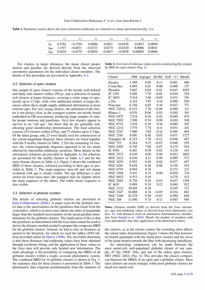
Table 1. Parameters used to derive the Gaia extinction coefficients as a function of colour and extinction (Eq. (1)).

c1 c2 c3 c4 c5 c6 c7

kG 0.9761 −0.1704 0.0086 0.0011 −0.0438 0.0013 0.0099kBP 1.1517 −0.0871 −0.0333 0.0173 −0.0230 0.0006 0.0043kRP 0.6104 −0.0170 −0.0026 −0.0017 −0.0078 0.00005 0.0006

For clusters at larger distances, the mean cluster propermotion and parallax are derived directly from the observedastrometric parameters for the individual cluster members. Thedetails of this procedure are presented in Appendix A.2.

3.2. Selection of open clusters

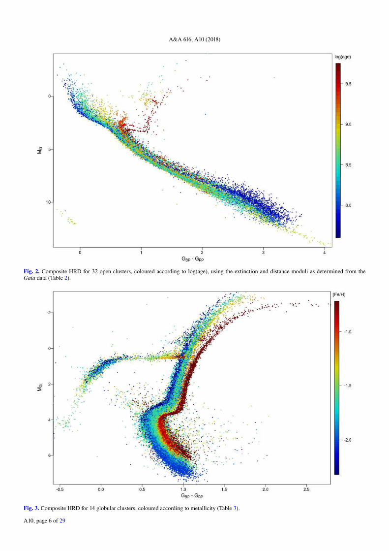
Our sample of open clusters consists of the mostly well-definedand fairly rich clusters within 250 pc, and a selection of mainlyrich clusters at larger distances, covering a wider range of ages,mostly up to 1.5 kpc, with a few additional clusters at larger dis-tances where these might supply additional information at moreextreme ages. For very young clusters, the definition of the clus-ter is not always clear, as the youngest systems are mostly foundembedded in OB associations, producing large samples of simi-lar proper motions and parallaxes. Very few clusters appear tosurvive to an “old age”, but those that do are generally rich,allowing good membership determination. The final selectionconsists of 9 clusters within 250 pc, and 37 clusters up to 5.3 kpc.Of the latter group, only 23 were finally used for construction ofthe colour-magnitude diagram; these clusters are listed togetherwith the 9 nearby clusters in Table 2. For the remaining 14 clus-ters, the colour-magnitude diagrams appeared to be too muchaffected by interstellar reddening variations. More details on theastrometric solutions are provided in Appendix A; the solutionsare presented for the nearby clusters in Table A.3 and for themore distant clusters in Table A.4. Figure 2 shows the combinedHRD of these clusters, coloured according to their ages as pro-vided in Table 2. The main-sequence turn-off and red clumpevolution with age is clearly visible. The age difference is alsoshown for lower mass stars, the youngest stars lie slightly abovethe main sequence of the others. The white dwarf sequence isalso visible.

3.3. Selection of globular clusters

The details of selecting globular clusters are presented inGaia Collaboration (2018c). A major issue for the globular clus-ter data is the uncertainties on the parallaxes that result from thesystematics, which is in most cases about one order of magnitudelarger than the standard uncertainties on the mean parallax deter-minations for the globular clusters. The implication of this is thatthe parallaxes as determined with the Gaia data cannot be used toderive the distance moduli needed to prepare the composite HRDfor the globular clusters. Instead, we had to rely on distances asquoted in the literature, for which we used the tables (2010 edi-tion) provided online by Harris (1996). The inevitable drawbackis that these distances and reddening values have been obtainedthrough isochrone fitting, and the application of these values tothe Gaia data will provide only limited new information. Themain advantage is the possibility of comparing the HRDs of allglobular clusters within a single, accurate photometric system.The combined HRD for 14 globular clusters is shown in Fig. 3,the summary data for these clusters is presented in Table 3. Thephotometric data originate predominantly from the outskirts of

Table 2. Overview of reference values used in constructing the compos-ite HRD for open clusters (Fig. 2).

Cluster DM log(age) [Fe/H] E(B − V) Memb

Hyades 3.389 8.90 0.13 0.001 480Coma Ber 4.669 8.81 0.00 0.000 127Pleiades 5.667 8.04 −0.01 0.045 1059IC 2391 5.908 7.70 −0.01 0.030 254IC 2602 5.914 7.60 −0.02 0.031 391α Per 6.214 7.85 0.14 0.090 598Praesepe 6.350 8.85 0.16 0.027 771NGC 2451A 6.433 7.78 −0.08 0.000 311Blanco 1 6.876 8.06 0.03 0.010 361NGC 6475 7.234 8.54 0.02 0.049 874NGC 7092 7.390 8.54 0.00 0.010 248NGC 6774 7.455 9.30 0.16 0.080 165NGC 2232 7.575 7.70 0.11 0.031 241NGC 2547 7.980 7.60 −0.14 0.040 404NGC 2516 8.091 8.48 0.05 0.071 1727Trumpler 10 8.223 7.78 −0.12 0.056 407NGC 752 8.264 9.15 −0.03 0.040 259NGC 6405 8.320 7.90 0.07 0.139 544IC 4756 8.401 8.98 0.02 0.128 515NGC 3532 8.430 8.60 0.00 0.022 1802NGC 2422 8.436 8.11 0.09 0.090 572NGC 1039 8.552 8.40 0.02 0.077 497NGC 6281 8.638 8.48 0.06 0.130 534NGC 6793 8.894 8.78 0.272 271NGC 2548 9.451 8.74 0.08 0.020 374NGC 6025 9.513 8.18 0.170 431NGC 2682 9.726 9.54 0.03 0.037 1194IC 4651 9.889 9.30 0.12 0.040 932NGC 2323 10.010 8.30 0.105 372NGC 2447 10.088 8.74 −0.05 0.034 681NGC 2360 10.229 8.98 −0.03 0.090 848NGC 188 11.490 9.74 0.11 0.085 956

Notes. Distance moduli (DM) as derived from the Gaia astrome-try; ages and reddening values as derived from Gaia photometry (seeSect. 6), with distances fixed on astrometric determinations; metallic-ities from Netopil et al. (2016); Memb: the number of members withGaia photometric data after application of the photometric filters.

the clusters, as in the cluster centres the crowding often affectsthe colour index determination. Figure 3 shows the blue horizon-tal branch populated with the metal-poor clusters and the moveof the giant branch towards the blue with decreasing metallicity.

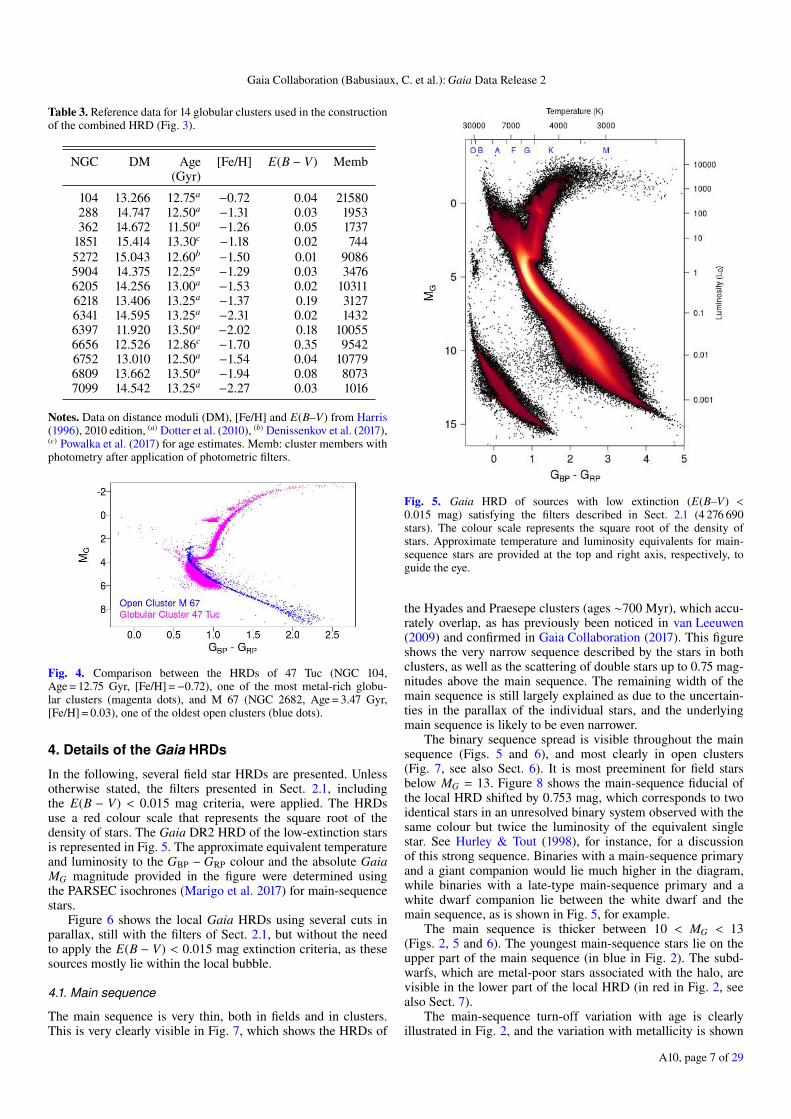
An interesting comparison can be made between themost metal-rich well-populated globular cluster of our sam-ple, 47 Tuc (NGC 104), and one of the oldest open clusters,M67 (NGC 2682) (Fig. 4). This provides the closest compari-son between the HRDs of an open and a globular cluster. Mostopen clusters are much younger, while most globular clusters aremuch less metal rich.

A10, page 5 of 29

A&A 616, A10 (2018)

Fig. 2. Composite HRD for 32 open clusters, coloured according to log(age), using the extinction and distance moduli as determined from theGaia data (Table 2).

Fig. 3. Composite HRD for 14 globular clusters, coloured according to metallicity (Table 3).

A10, page 6 of 29

Gaia Collaboration (Babusiaux, C. et al.): Gaia Data Release 2

Table 3. Reference data for 14 globular clusters used in the constructionof the combined HRD (Fig. 3).

NGC DM Age [Fe/H] E(B − V) Memb(Gyr)

104 13.266 12.75a −0.72 0.04 21580288 14.747 12.50a −1.31 0.03 1953362 14.672 11.50a −1.26 0.05 1737

1851 15.414 13.30c −1.18 0.02 7445272 15.043 12.60b −1.50 0.01 90865904 14.375 12.25a −1.29 0.03 34766205 14.256 13.00a −1.53 0.02 103116218 13.406 13.25a −1.37 0.19 31276341 14.595 13.25a −2.31 0.02 14326397 11.920 13.50a −2.02 0.18 100556656 12.526 12.86c −1.70 0.35 95426752 13.010 12.50a −1.54 0.04 107796809 13.662 13.50a −1.94 0.08 80737099 14.542 13.25a −2.27 0.03 1016

Notes. Data on distance moduli (DM), [Fe/H] and E(B–V) from Harris(1996), 2010 edition, (a) Dotter et al. (2010), (b) Denissenkov et al. (2017),(c) Powalka et al. (2017) for age estimates. Memb: cluster members withphotometry after application of photometric filters.

Fig. 4. Comparison between the HRDs of 47 Tuc (NGC 104,Age = 12.75 Gyr, [Fe/H] =−0.72), one of the most metal-rich globu-lar clusters (magenta dots), and M 67 (NGC 2682, Age = 3.47 Gyr,[Fe/H] = 0.03), one of the oldest open clusters (blue dots).

4. Details of the Gaia HRDs

In the following, several field star HRDs are presented. Unlessotherwise stated, the filters presented in Sect. 2.1, includingthe E(B − V) < 0.015 mag criteria, were applied. The HRDsuse a red colour scale that represents the square root of thedensity of stars. The Gaia DR2 HRD of the low-extinction starsis represented in Fig. 5. The approximate equivalent temperatureand luminosity to the GBP − GRP colour and the absolute GaiaMG magnitude provided in the figure were determined usingthe PARSEC isochrones (Marigo et al. 2017) for main-sequencestars.

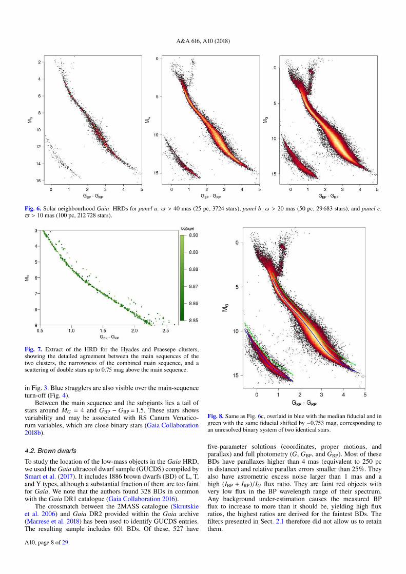
Figure 6 shows the local Gaia HRDs using several cuts inparallax, still with the filters of Sect. 2.1, but without the needto apply the E(B − V) < 0.015 mag extinction criteria, as thesesources mostly lie within the local bubble.

4.1. Main sequence

The main sequence is very thin, both in fields and in clusters.This is very clearly visible in Fig. 7, which shows the HRDs of

Fig. 5. Gaia HRD of sources with low extinction (E(B–V) <0.015 mag) satisfying the filters described in Sect. 2.1 (4 276 690stars). The colour scale represents the square root of the density ofstars. Approximate temperature and luminosity equivalents for main-sequence stars are provided at the top and right axis, respectively, toguide the eye.

the Hyades and Praesepe clusters (ages ∼700 Myr), which accu-rately overlap, as has previously been noticed in van Leeuwen(2009) and confirmed in Gaia Collaboration (2017). This figureshows the very narrow sequence described by the stars in bothclusters, as well as the scattering of double stars up to 0.75 mag-nitudes above the main sequence. The remaining width of themain sequence is still largely explained as due to the uncertain-ties in the parallax of the individual stars, and the underlyingmain sequence is likely to be even narrower.

The binary sequence spread is visible throughout the mainsequence (Figs. 5 and 6), and most clearly in open clusters(Fig. 7, see also Sect. 6). It is most preeminent for field starsbelow MG = 13. Figure 8 shows the main-sequence fiducial ofthe local HRD shifted by 0.753 mag, which corresponds to twoidentical stars in an unresolved binary system observed with thesame colour but twice the luminosity of the equivalent singlestar. See Hurley & Tout (1998), for instance, for a discussionof this strong sequence. Binaries with a main-sequence primaryand a giant companion would lie much higher in the diagram,while binaries with a late-type main-sequence primary and awhite dwarf companion lie between the white dwarf and themain sequence, as is shown in Fig. 5, for example.

The main sequence is thicker between 10 < MG < 13(Figs. 2, 5 and 6). The youngest main-sequence stars lie on theupper part of the main sequence (in blue in Fig. 2). The subd-warfs, which are metal-poor stars associated with the halo, arevisible in the lower part of the local HRD (in red in Fig. 2, seealso Sect. 7).

The main-sequence turn-off variation with age is clearlyillustrated in Fig. 2, and the variation with metallicity is shown

A10, page 7 of 29

A&A 616, A10 (2018)

Fig. 6. Solar neighbourhood Gaia HRDs for panel a: > 40 mas (25 pc, 3724 stars), panel b: > 20 mas (50 pc, 29 683 stars), and panel c: > 10 mas (100 pc, 212 728 stars).

Fig. 7. Extract of the HRD for the Hyades and Praesepe clusters,showing the detailed agreement between the main sequences of thetwo clusters, the narrowness of the combined main sequence, and ascattering of double stars up to 0.75 mag above the main sequence.

in Fig. 3. Blue stragglers are also visible over the main-sequenceturn-off (Fig. 4).

Between the main sequence and the subgiants lies a tail ofstars around MG = 4 and GBP − GRP = 1.5. These stars showsvariability and may be associated with RS Canum Venatico-rum variables, which are close binary stars (Gaia Collaboration2018b).

4.2. Brown dwarfs

To study the location of the low-mass objects in the Gaia HRD,we used the Gaia ultracool dwarf sample (GUCDS) compiled bySmart et al. (2017). It includes 1886 brown dwarfs (BD) of L, T,and Y types, although a substantial fraction of them are too faintfor Gaia. We note that the authors found 328 BDs in commonwith the Gaia DR1 catalogue (Gaia Collaboration 2016).

The crossmatch between the 2MASS catalogue (Skrutskieet al. 2006) and Gaia DR2 provided within the Gaia archive(Marrese et al. 2018) has been used to identify GUCDS entries.The resulting sample includes 601 BDs. Of these, 527 have

Fig. 8. Same as Fig. 6c, overlaid in blue with the median fiducial and ingreen with the same fiducial shifted by −0.753 mag, corresponding toan unresolved binary system of two identical stars.

five-parameter solutions (coordinates, proper motions, andparallax) and full photometry (G, GBP, and GRP). Most of theseBDs have parallaxes higher than 4 mas (equivalent to 250 pcin distance) and relative parallax errors smaller than 25%. Theyalso have astrometric excess noise larger than 1 mas and ahigh (IBP + IRP)/IG flux ratio. They are faint red objects withvery low flux in the BP wavelength range of their spectrum.Any background under-estimation causes the measured BPflux to increase to more than it should be, yielding high fluxratios, the highest ratios are derived for the faintest BDs. Thefilters presented in Sect. 2.1 therefore did not allow us to retainthem.

A10, page 8 of 29

Gaia Collaboration (Babusiaux, C. et al.): Gaia Data Release 2

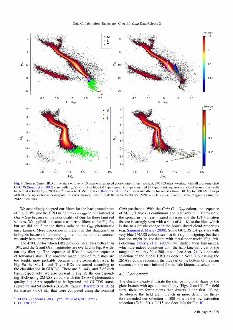
Fig. 9. Panel a: Gaia HRD of the stars with > 10 mas with adapted photometric filters (see text, 240 703 stars) overlaid with all cross-matchedGUCDS (Smart et al. 2017) stars with σ/ < 10% in blue (M type), green (L type), and red (T type). Pink squares are added around stars withtangential velocity VT > 200 km s−1. Panel b: BT-Settl tracks (Baraffe et al. 2015) of solar metallicity for masses from 0.01 M⊙ to 0.08 M⊙ in stepsof 0.01 (the upper tracks correspond to lower masses) plus in pink the same tracks for [M/H] =−1.0. Panels c and d: same diagrams using the2MASS colours.

We accordingly adapted our filters for the background starsof Fig. 9. We plot the HRD using the G −GRP colour instead ofGBP −GRP because of the poor quality of GBP for these faint redsources. We applied the same astrometric filters as for Fig. 6c,but we did not filter the fluxes ratio or the GBP photometricuncertainties. More dispersion is present in this diagram thanin Fig. 6c because of this missing filter, but the faint red sourceswe study here are represented better.

The 470 BDs for which DR2 provides parallaxes better than10%, and the G and GRP magnitudes are overlaid in Fig. 9 with-out any filtering. The sequence of BDs follows the sequenceof low-mass stars. The absolute magnitudes of four stars aretoo bright, most probably because of a cross-match issue. InFig. 9a the M-, L- and T-type BDs are sorted according tothe classification in GUCDS. There are 21, 443, and 7 of eachtype, respectively. We also present in Fig. 9c the correspond-ing HRD using 2MASS colours with the 2MASS photometricquality flag AAA (applied to background and GUCDS stars).Figure 9b and 9d includes BT-Settl tracks2 (Baraffe et al. 2015)for masses <0.08 M⊙ that were computed using the nominal

2 https://phoenix.ens-lyon.fr/Grids/BT-Settl/

CIFIST2011bc

Gaia passbands. With the Gaia G − GRP colour, the sequenceof M, L, T types is continuous and relatively thin. Conversely,the spread in the near-infrared is larger and the L/T transitionfeature is strongly seen with a shift of J − Ks to the blue, whichis due to a drastic change in the brown dwarf cloud properties(e.g. Saumon & Marley 2008). Some GUCDS L-type stars withvery blue 2MASS colours seem at first sight intriguing, but theirlocation might be consistent with metal-poor tracks (Fig. 9d).Following Faherty et al. (2009), we studied their kinematics,which are indeed consistent with the halo kinematic cut of thetangential velocity VT > 200 km s−1 (see Sect. 7). A kinematicselection of the global HRD as done in Sect. 7 but using the2MASS colours confirms the blue tail of the bottom of the mainsequence in the near-infrared for the halo kinematic selection.

4.3. Giant branch

The clusters clearly illustrate the change in global shape of thegiant branch with age and metallicity (Figs. 2 and 3). For fieldstars, there are fewer giants than dwarfs in the first 100 pc.To observe the field giant branch in more detail, we there-fore extended our selection to 500 pc with the low-extinctionselection (E(B − V) < 0.015, see Sect. 2.2) for Fig. 10.

A10, page 9 of 29

A&A 616, A10 (2018)

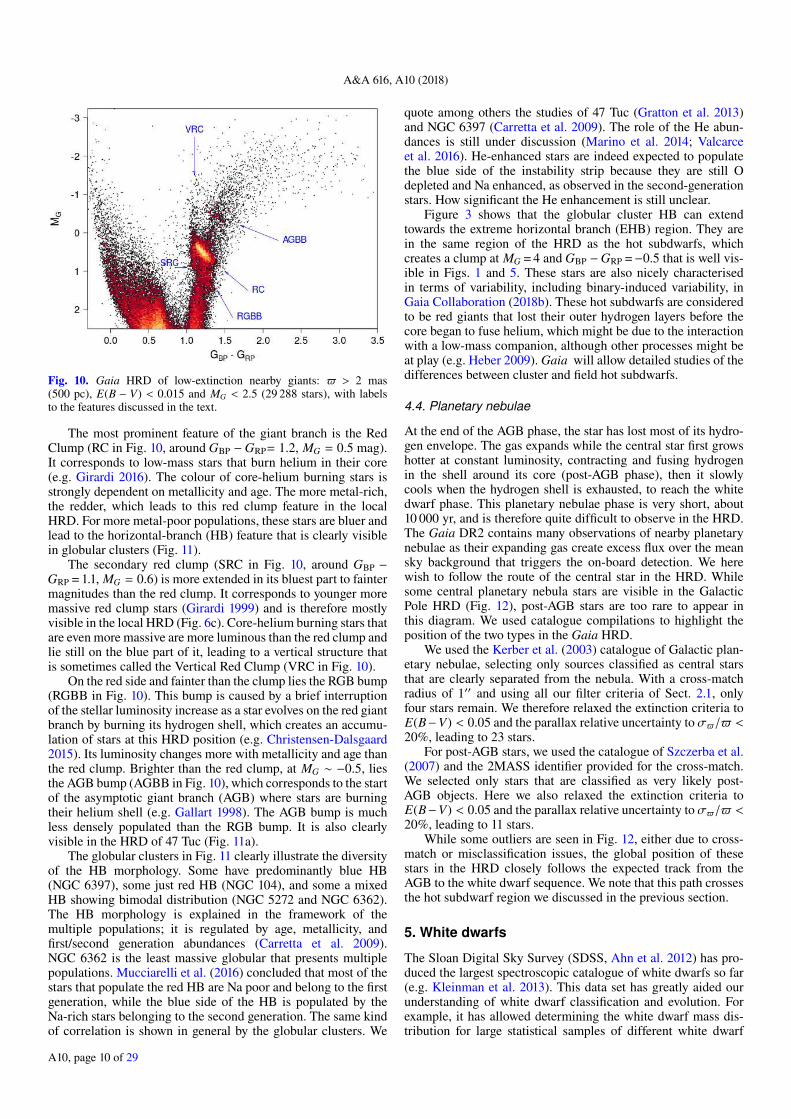
Fig. 10. Gaia HRD of low-extinction nearby giants: > 2 mas(500 pc), E(B − V) < 0.015 and MG < 2.5 (29 288 stars), with labelsto the features discussed in the text.

The most prominent feature of the giant branch is the RedClump (RC in Fig. 10, around GBP −GRP= 1.2, MG = 0.5 mag).It corresponds to low-mass stars that burn helium in their core(e.g. Girardi 2016). The colour of core-helium burning stars isstrongly dependent on metallicity and age. The more metal-rich,the redder, which leads to this red clump feature in the localHRD. For more metal-poor populations, these stars are bluer andlead to the horizontal-branch (HB) feature that is clearly visiblein globular clusters (Fig. 11).

The secondary red clump (SRC in Fig. 10, around GBP −

GRP = 1.1, MG = 0.6) is more extended in its bluest part to faintermagnitudes than the red clump. It corresponds to younger moremassive red clump stars (Girardi 1999) and is therefore mostlyvisible in the local HRD (Fig. 6c). Core-helium burning stars thatare even more massive are more luminous than the red clump andlie still on the blue part of it, leading to a vertical structure thatis sometimes called the Vertical Red Clump (VRC in Fig. 10).

On the red side and fainter than the clump lies the RGB bump(RGBB in Fig. 10). This bump is caused by a brief interruptionof the stellar luminosity increase as a star evolves on the red giantbranch by burning its hydrogen shell, which creates an accumu-lation of stars at this HRD position (e.g. Christensen-Dalsgaard2015). Its luminosity changes more with metallicity and age thanthe red clump. Brighter than the red clump, at MG ∼ −0.5, liesthe AGB bump (AGBB in Fig. 10), which corresponds to the startof the asymptotic giant branch (AGB) where stars are burningtheir helium shell (e.g. Gallart 1998). The AGB bump is muchless densely populated than the RGB bump. It is also clearlyvisible in the HRD of 47 Tuc (Fig. 11a).

The globular clusters in Fig. 11 clearly illustrate the diversityof the HB morphology. Some have predominantly blue HB(NGC 6397), some just red HB (NGC 104), and some a mixedHB showing bimodal distribution (NGC 5272 and NGC 6362).The HB morphology is explained in the framework of themultiple populations; it is regulated by age, metallicity, andfirst/second generation abundances (Carretta et al. 2009).NGC 6362 is the least massive globular that presents multiplepopulations. Mucciarelli et al. (2016) concluded that most of thestars that populate the red HB are Na poor and belong to the firstgeneration, while the blue side of the HB is populated by theNa-rich stars belonging to the second generation. The same kindof correlation is shown in general by the globular clusters. We

quote among others the studies of 47 Tuc (Gratton et al. 2013)and NGC 6397 (Carretta et al. 2009). The role of the He abun-dances is still under discussion (Marino et al. 2014; Valcarceet al. 2016). He-enhanced stars are indeed expected to populatethe blue side of the instability strip because they are still Odepleted and Na enhanced, as observed in the second-generationstars. How significant the He enhancement is still unclear.

Figure 3 shows that the globular cluster HB can extendtowards the extreme horizontal branch (EHB) region. They arein the same region of the HRD as the hot subdwarfs, whichcreates a clump at MG = 4 and GBP −GRP =−0.5 that is well vis-ible in Figs. 1 and 5. These stars are also nicely characterisedin terms of variability, including binary-induced variability, inGaia Collaboration (2018b). These hot subdwarfs are consideredto be red giants that lost their outer hydrogen layers before thecore began to fuse helium, which might be due to the interactionwith a low-mass companion, although other processes might beat play (e.g. Heber 2009). Gaia will allow detailed studies of thedifferences between cluster and field hot subdwarfs.

4.4. Planetary nebulae

At the end of the AGB phase, the star has lost most of its hydro-gen envelope. The gas expands while the central star first growshotter at constant luminosity, contracting and fusing hydrogenin the shell around its core (post-AGB phase), then it slowlycools when the hydrogen shell is exhausted, to reach the whitedwarf phase. This planetary nebulae phase is very short, about10 000 yr, and is therefore quite difficult to observe in the HRD.The Gaia DR2 contains many observations of nearby planetarynebulae as their expanding gas create excess flux over the meansky background that triggers the on-board detection. We herewish to follow the route of the central star in the HRD. Whilesome central planetary nebula stars are visible in the GalacticPole HRD (Fig. 12), post-AGB stars are too rare to appear inthis diagram. We used catalogue compilations to highlight theposition of the two types in the Gaia HRD.

We used the Kerber et al. (2003) catalogue of Galactic plan-etary nebulae, selecting only sources classified as central starsthat are clearly separated from the nebula. With a cross-matchradius of 1′′ and using all our filter criteria of Sect. 2.1, onlyfour stars remain. We therefore relaxed the extinction criteria toE(B−V) < 0.05 and the parallax relative uncertainty to σ/ <20%, leading to 23 stars.

For post-AGB stars, we used the catalogue of Szczerba et al.(2007) and the 2MASS identifier provided for the cross-match.We selected only stars that are classified as very likely post-AGB objects. Here we also relaxed the extinction criteria toE(B−V) < 0.05 and the parallax relative uncertainty to σ/ <20%, leading to 11 stars.

While some outliers are seen in Fig. 12, either due to cross-match or misclassification issues, the global position of thesestars in the HRD closely follows the expected track from theAGB to the white dwarf sequence. We note that this path crossesthe hot subdwarf region we discussed in the previous section.

5. White dwarfs

The Sloan Digital Sky Survey (SDSS, Ahn et al. 2012) has pro-duced the largest spectroscopic catalogue of white dwarfs so far(e.g. Kleinman et al. 2013). This data set has greatly aided ourunderstanding of white dwarf classification and evolution. Forexample, it has allowed determining the white dwarf mass dis-tribution for large statistical samples of different white dwarf

A10, page 10 of 29

Gaia Collaboration (Babusiaux, C. et al.): Gaia Data Release 2

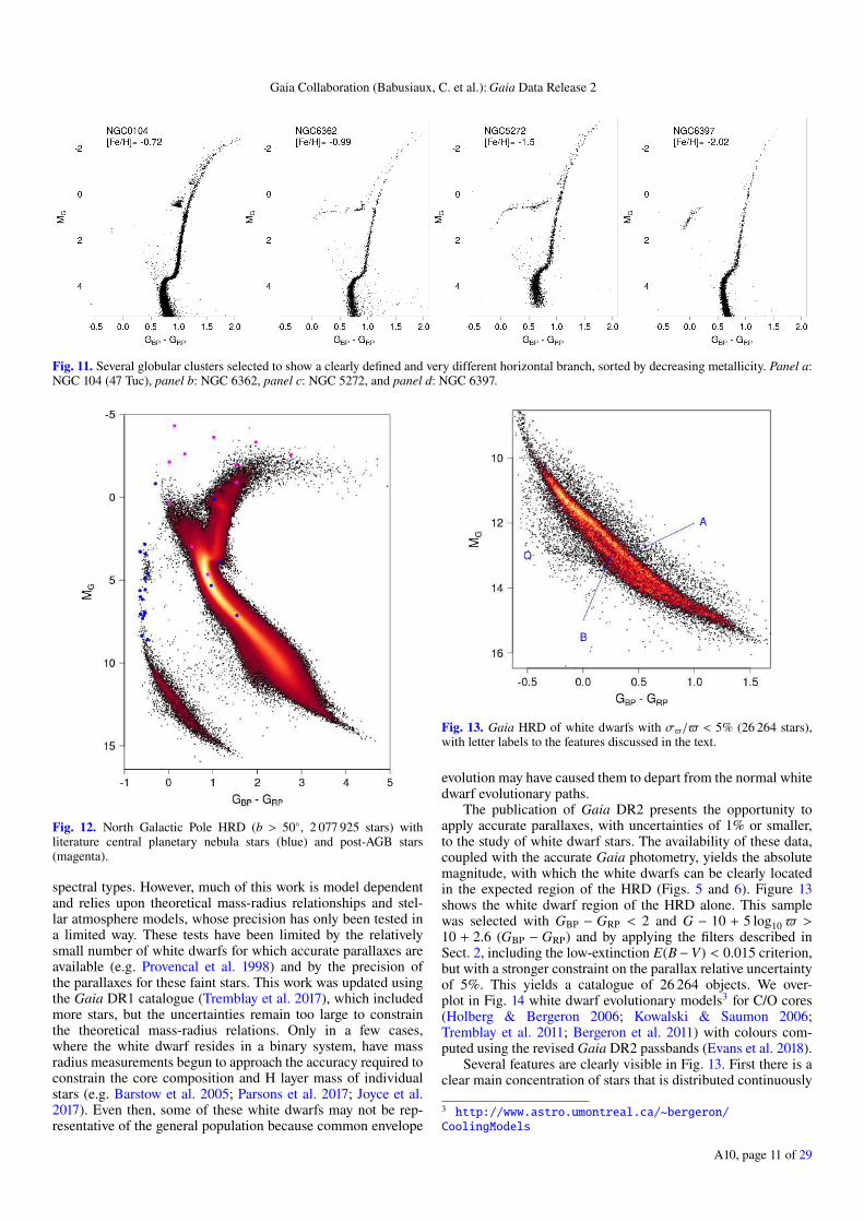
Fig. 11. Several globular clusters selected to show a clearly defined and very different horizontal branch, sorted by decreasing metallicity. Panel a:NGC 104 (47 Tuc), panel b: NGC 6362, panel c: NGC 5272, and panel d: NGC 6397.

Fig. 12. North Galactic Pole HRD (b > 50◦, 2 077 925 stars) withliterature central planetary nebula stars (blue) and post-AGB stars(magenta).

spectral types. However, much of this work is model dependentand relies upon theoretical mass-radius relationships and stel-lar atmosphere models, whose precision has only been tested ina limited way. These tests have been limited by the relativelysmall number of white dwarfs for which accurate parallaxes areavailable (e.g. Provencal et al. 1998) and by the precision ofthe parallaxes for these faint stars. This work was updated usingthe Gaia DR1 catalogue (Tremblay et al. 2017), which includedmore stars, but the uncertainties remain too large to constrainthe theoretical mass-radius relations. Only in a few cases,where the white dwarf resides in a binary system, have massradius measurements begun to approach the accuracy required toconstrain the core composition and H layer mass of individualstars (e.g. Barstow et al. 2005; Parsons et al. 2017; Joyce et al.2017). Even then, some of these white dwarfs may not be rep-resentative of the general population because common envelope

Fig. 13. Gaia HRD of white dwarfs with σ/ < 5% (26 264 stars),with letter labels to the features discussed in the text.

evolution may have caused them to depart from the normal whitedwarf evolutionary paths.

The publication of Gaia DR2 presents the opportunity toapply accurate parallaxes, with uncertainties of 1% or smaller,to the study of white dwarf stars. The availability of these data,coupled with the accurate Gaia photometry, yields the absolutemagnitude, with which the white dwarfs can be clearly locatedin the expected region of the HRD (Figs. 5 and 6). Figure 13shows the white dwarf region of the HRD alone. This samplewas selected with GBP − GRP < 2 and G − 10 + 5 log10 >10 + 2.6 (GBP − GRP) and by applying the filters described inSect. 2, including the low-extinction E(B−V) < 0.015 criterion,but with a stronger constraint on the parallax relative uncertaintyof 5%. This yields a catalogue of 26 264 objects. We over-plot in Fig. 14 white dwarf evolutionary models3 for C/O cores(Holberg & Bergeron 2006; Kowalski & Saumon 2006;Tremblay et al. 2011; Bergeron et al. 2011) with colours com-puted using the revised Gaia DR2 passbands (Evans et al. 2018).

Several features are clearly visible in Fig. 13. First there is aclear main concentration of stars that is distributed continuously

3 http://www.astro.umontreal.ca/~bergeron/

CoolingModels

A10, page 11 of 29

A&A 616, A10 (2018)

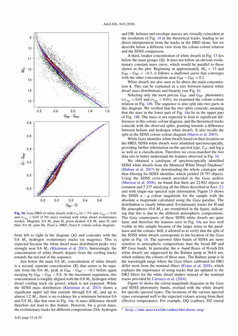
Fig. 14. Gaia HRD of white dwarfs with σ/ < 5% and σGBP < 0.01and σGRP < 0.01 (5 781 stars) overlaid with white dwarf evolutionarymodels. Magenta: 0.6 M⊙ pure H; green dashed: 0.8 M⊙ pure H; andblue: 0.6 M⊙ pure He. Panel a: HRD. Panel b: colour–colour diagram.

from left to right in the diagram (A) and coincides with the0.6 M⊙ hydrogen evolutionary tracks (in magenta). This isexpected because the white dwarf mass distribution peaks verystrongly near 0.6 M⊙ (Kleinman et al. 2013). Interestingly, theconcentration of white dwarfs departs from the cooling trackstowards the red end of the sequence.

Just below the main 0.6 M⊙ concentration of white dwarfsis a second, separate concentration (B) that seems to be sepa-rate from the 0.6 M⊙ peak at GBP − GRP ∼ −0.1 before againmerging by GBP −GRP ∼ 0.8. At the maximum separation, thisconcentration is roughly aligned with the 0.8 M⊙ hydrogen whitedwarf cooling track (in green), which is not expected. Whilethe SDSS mass distribution (Kleinman et al. 2013) shows asignificant upper tail that extends through 0.8 M⊙ and up toalmost 1.2 M⊙, there is no evidence for a minimum between 0.6and 0.8 M⊙ like that seen in Fig. 14a. A mass difference shouldtherefore not lead to this feature. However, for a given mass,the evolutionary tracks for different compositions (DA: hydrogen

and DB: helium) and envelope masses are virtually coincident atthe resolution of Fig. 14 in the theoretical tracks, leading to nodirect interpretation from the tracks in the HRD alone, but wedescribe below a different view from the colour–colour relationand the SDSS comparison.

A third, weaker concentration of white dwarfs in Fig. 13 liesbelow the main groups (Q). It does not follow an obvious evolu-tionary constant mass curve, which would be parallel to thoseshown in the plot. Beginning at approximately MG = 13 andGBP − GRP = −0.3, it follows a shallower curve that convergeswith the other concentrations near GBP −GRP = 0.2.

White dwarfs are also seen to lie above the main concentra-tion A. This can be explained as a mix between natural whitedwarf mass distributions and binarity (see Fig. 8).

Selecting only the most precise GBP and GRP photometry(σGBP < 0.01 and σGRP < 0.01), we examined the colour–colourrelation in Fig. 14b. The sequence is also split into two parts inthis diagram. We verified that the two splits coincide, meaningthat the stars in the lower part of Fig. 14a lie in the upper partof Fig. 14b. The mass is not expected to lead to significant dif-ferences in this colour–colour diagram, and the theoretical trackscoincide with the observed splits, pointing towards a differencebetween helium and hydrogen white dwarfs. It also recalls thesplit in the SDSS colour–colour diagram (Harris et al. 2003).

While Gaia identifies white dwarfs based on their location onthe HRD, SDSS white dwarfs were identified spectroscopically,providing further information on the spectral type, Teff , and log gas well as a classification. Therefore we cross-matched the twodata sets to better understand the features observed in Fig. 14.

We obtained a catalogue of spectroscopically identifiedSDSS white dwarfs from the Montreal White Dwarf Database4

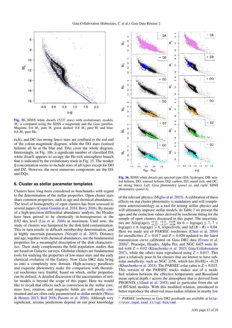
(Dufour et al. 2017) by downloading the whole catalogue andthen filtering for SDSS identifier, which yielded 28 797 objects.Using the SDSS cross-match provided in the Gaia archive(Marrese et al. 2018), we found that there are 22 802 objects incommon and 5 237 satisfying all the filters described in Sect. 2.1and with single-star spectral type information. Figure 15 showsthe SDSS u − g colour magnitude for the sample with theabsolute u magnitude calculated using the Gaia parallax. Thedistribution is clearly bifurcated. Evolutionary tracks for H andHe atmospheres (0.6 M⊙) are overplotted in the figure, indicat-ing that this is due to the different atmospheric compositions.The Gaia counterparts of these SDSS white dwarfs are quitefaint, and therefore the features seen in Fig. 14a are less wellvisible in this sample because of the larger noise in the paral-laxes and the colours. Still, it allowed us to verify that the split ofthe SDSS white dwarfs corresponds to the location of the Gaiasplits in Fig. 14. The narrower filter bands of SDSS are moresensitive to atmospheric compositions than the broad BP andRP Gaia bands. In particular, the u -band fluxes of H-rich DAwhite dwarfs are suppressed by the Balmer jump at 364.6 nm,which reddens the colours of these stars. The Balmer jump is inthe wavelength range where the Gaia filters calibrated for DR2differ most from the nominal filters (Evans et al. 2018), whichexplains the importance of using tracks that are updated to theDR2 filters for the white dwarf studies instead of the nominaltracks provided by Carrasco et al. (2014).

Figure 16 shows the colour-magnitude diagrams in the Gaiaand SDSS photometry bands, overlaid with the white dwarfsfor specific spectral types. The locations of the various spectraltypes correspond well to the expected colours arising from theireffective temperatures. For example, DQ (carbon), DZ (metal

4 http://www.montrealwhitedwarfdatabase.org/

A10, page 12 of 29

Gaia Collaboration (Babusiaux, C. et al.): Gaia Data Release 2

Fig. 15. SDSS white dwarfs (5237 stars) with evolutionary models.Mu is computed using the SDSS u magnitude and the Gaia parallax.Magenta: 0.6 M⊙ pure H; green dashed: 0.8 M⊙ pure H; and blue:0.6 M⊙ pure He.

rich), and DC (no strong lines) stars are confined to the red endof the colour-magnitude diagram, while the DO stars (ionisedhelium) all lie at the blue end. DAs cover the whole diagram.Interestingly, in Fig. 16b, a significant number of classified DAwhite dwarfs appears to occupy the He-rich atmosphere branchthat is indicated by the evolutionary track in Fig. 15. The weakerQ concentration seems to include stars of all types except for DOand DZ. However, the most numerous components are the DAand DQs.

6. Cluster as stellar parameter templates

Clusters have long been considered as benchmarks with regardto the determination of the stellar properties. Open cluster starsshare common properties, such as age and chemical abundances.The level of homogeneity of open clusters has been assessed inseveral papers (Cantat-Gaudin et al. 2014; Bovy 2016). By meansof a high-precision differential abundance analysis, the Hyadeshave been proved to be chemically in-homogeneous at the0.02 dex level (Liu et al. 2016) at maximum. Until now, thestudy of clusters was hampered by the disk field contamination.This in turn results in difficult membership determination, andin highly uncertain parameters (Netopil et al. 2015). Distanceand age, together with chemical abundances, are the fundamentalproperties for a meaningful description of the disk characteris-tics. Their study complements the field population studies thatare based on Galactic surveys. Globular clusters are fundamentaltools for studying the properties of low-mass stars and the earlychemical evolution of the Galaxy. Now Gaia DR2 data bringus into a completely new domain. High-accuracy parallaxesand exquisite photometry make the comparison with theoreti-cal isochrones very fruitful, based on which, stellar propertiescan be defined. A detailed discussion of the uncertainties of stel-lar models is beyond the scope of this paper. Here we wouldlike to recall that effects such as convection in the stellar core,mass loss, rotation, and magnetic fields are still poorly con-strained and are often only parametrised in stellar models (Weiss& Heners 2013; Bell 2016; Pasetto et al. 2016). Although verysignificant, seismic predictions depend on our poor knowledge

Fig. 16. SDSS white dwarfs per spectral type (DA: hydrogen; DB: neu-tral helium; DO: ionised helium; DQ: carbon; DZ: metal rich; and DC:no strong lines). Left: Gaia photometry (panel a), and right: SDSSphotometry (panel b).

of the relevant physics (Miglio et al. 2015). A calibration of theseeffects on star cluster photometry is mandatory and will comple-ment asteroseismology as a tool for testing stellar physics andwill ultimately improve stellar models. In Table 2 we present theages and the extinction values derived by isochrone fitting for thesample of open clusters discussed in this paper. The uncertain-ties are ∆(log(age)) +0.14

−0.22, +0.11−0.13, +0.08

−0.06 for 6 < log(age) ≤ 7, 7 <log(age) ≤ 8, log(age) > 8, respectively, and ∆E(B − R) = 0.04.Here we made use of PARSEC isochrones (Chen et al. 2014)for metallicities Z = 0.017 and Z = 0.020 updated to the latesttransmission curve calibrated on Gaia DR2 data (Evans et al.2018)5. Praesepe, Hyades, Alpha Per, and NGC 6475 were fit-ted with Z = 0.02 (Kharchenko et al. 2015; Gaia Collaboration2017), while the others were reproduced using Z = 0.017. Thisgave a relatively poor fit for clusters that are known to have sub-solar metallicity, such as NGC 2158, which has [Fe/H] =−0.25(Kharchenko et al. 2015). The PARSEC solar value is Z = 0.015.This version of the PARSEC tracks makes use of a modi-fied relation between the effective temperature and Rosselandmean optical depth τ across the atmosphere that is derived fromPHOENIX (Allard et al. 2012) and in particular from the setof BT-Settl models. With this modified relation, introduced tobetter reproduce the observed mass-radius relation in nearby low

5 PARSEC isochrones in Gaia DR2 passbands are available at http://stev.oapd.inaf.it/cgi-bin/cmd

A10, page 13 of 29

A&A 616, A10 (2018)

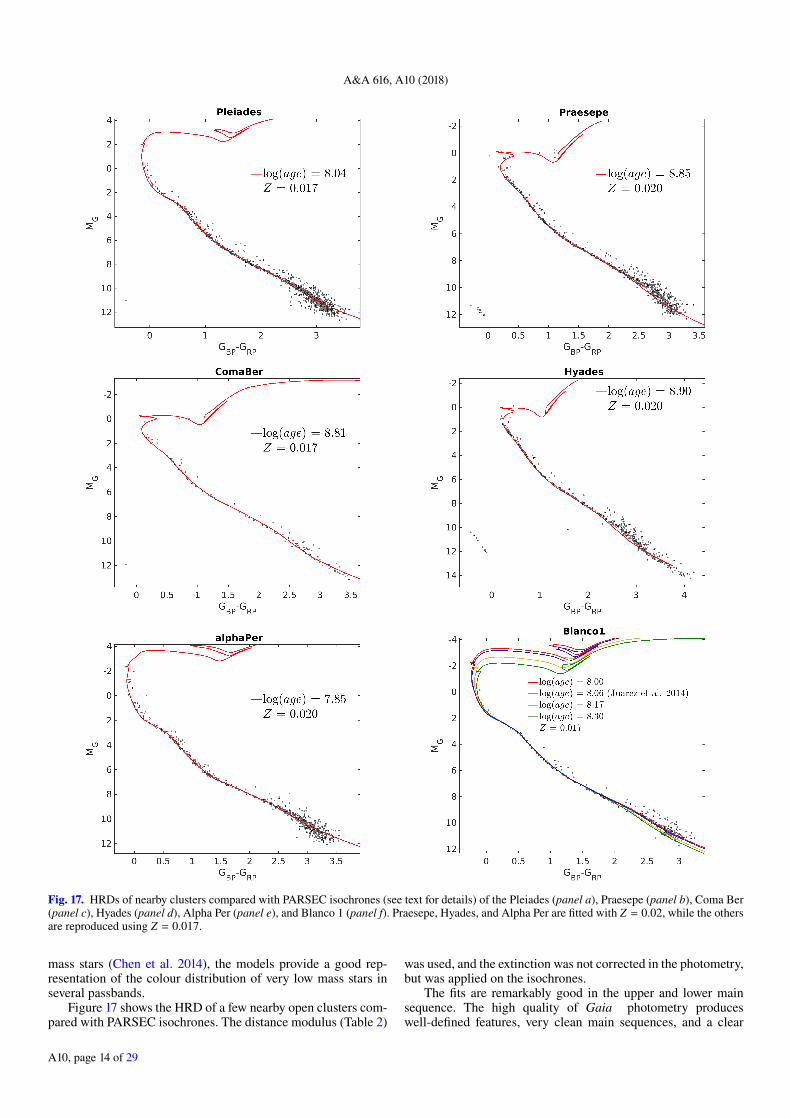
Fig. 17. HRDs of nearby clusters compared with PARSEC isochrones (see text for details) of the Pleiades (panel a), Praesepe (panel b), Coma Ber(panel c), Hyades (panel d), Alpha Per (panel e), and Blanco 1 (panel f). Praesepe, Hyades, and Alpha Per are fitted with Z = 0.02, while the othersare reproduced using Z = 0.017.

mass stars (Chen et al. 2014), the models provide a good rep-resentation of the colour distribution of very low mass stars inseveral passbands.

Figure 17 shows the HRD of a few nearby open clusters com-pared with PARSEC isochrones. The distance modulus (Table 2)

was used, and the extinction was not corrected in the photometry,but was applied on the isochrones.

The fits are remarkably good in the upper and lower mainsequence. The high quality of Gaia photometry produceswell-defined features, very clean main sequences, and a clear

A10, page 14 of 29

Gaia Collaboration (Babusiaux, C. et al.): Gaia Data Release 2

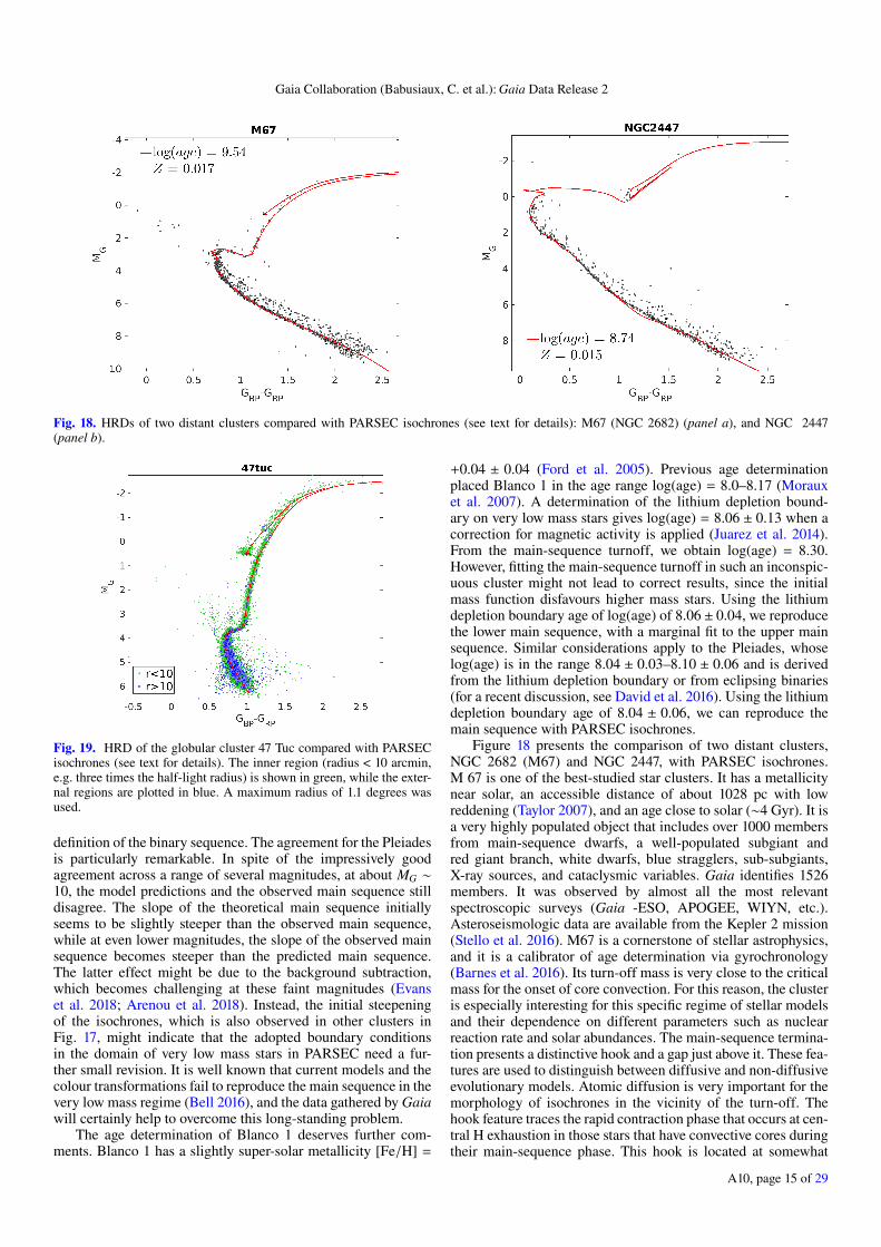
Fig. 18. HRDs of two distant clusters compared with PARSEC isochrones (see text for details): M67 (NGC 2682) (panel a), and NGC 2447(panel b).

Fig. 19. HRD of the globular cluster 47 Tuc compared with PARSECisochrones (see text for details). The inner region (radius < 10 arcmin,e.g. three times the half-light radius) is shown in green, while the exter-nal regions are plotted in blue. A maximum radius of 1.1 degrees wasused.

definition of the binary sequence. The agreement for the Pleiadesis particularly remarkable. In spite of the impressively goodagreement across a range of several magnitudes, at about MG ∼

10, the model predictions and the observed main sequence stilldisagree. The slope of the theoretical main sequence initiallyseems to be slightly steeper than the observed main sequence,while at even lower magnitudes, the slope of the observed mainsequence becomes steeper than the predicted main sequence.The latter effect might be due to the background subtraction,which becomes challenging at these faint magnitudes (Evanset al. 2018; Arenou et al. 2018). Instead, the initial steepeningof the isochrones, which is also observed in other clusters inFig. 17, might indicate that the adopted boundary conditionsin the domain of very low mass stars in PARSEC need a fur-ther small revision. It is well known that current models and thecolour transformations fail to reproduce the main sequence in thevery low mass regime (Bell 2016), and the data gathered by Gaiawill certainly help to overcome this long-standing problem.

The age determination of Blanco 1 deserves further com-ments. Blanco 1 has a slightly super-solar metallicity [Fe/H] =

+0.04 ± 0.04 (Ford et al. 2005). Previous age determinationplaced Blanco 1 in the age range log(age) = 8.0–8.17 (Morauxet al. 2007). A determination of the lithium depletion bound-ary on very low mass stars gives log(age) = 8.06 ± 0.13 when acorrection for magnetic activity is applied (Juarez et al. 2014).From the main-sequence turnoff, we obtain log(age) = 8.30.However, fitting the main-sequence turnoff in such an inconspic-uous cluster might not lead to correct results, since the initialmass function disfavours higher mass stars. Using the lithiumdepletion boundary age of log(age) of 8.06 ± 0.04, we reproducethe lower main sequence, with a marginal fit to the upper mainsequence. Similar considerations apply to the Pleiades, whoselog(age) is in the range 8.04 ± 0.03–8.10 ± 0.06 and is derivedfrom the lithium depletion boundary or from eclipsing binaries(for a recent discussion, see David et al. 2016). Using the lithiumdepletion boundary age of 8.04 ± 0.06, we can reproduce themain sequence with PARSEC isochrones.

Figure 18 presents the comparison of two distant clusters,NGC 2682 (M67) and NGC 2447, with PARSEC isochrones.M 67 is one of the best-studied star clusters. It has a metallicitynear solar, an accessible distance of about 1028 pc with lowreddening (Taylor 2007), and an age close to solar (∼4 Gyr). It isa very highly populated object that includes over 1000 membersfrom main-sequence dwarfs, a well-populated subgiant andred giant branch, white dwarfs, blue stragglers, sub-subgiants,X-ray sources, and cataclysmic variables. Gaia identifies 1526members. It was observed by almost all the most relevantspectroscopic surveys (Gaia -ESO, APOGEE, WIYN, etc.).Asteroseismologic data are available from the Kepler 2 mission(Stello et al. 2016). M67 is a cornerstone of stellar astrophysics,and it is a calibrator of age determination via gyrochronology(Barnes et al. 2016). Its turn-off mass is very close to the criticalmass for the onset of core convection. For this reason, the clusteris especially interesting for this specific regime of stellar modelsand their dependence on different parameters such as nuclearreaction rate and solar abundances. The main-sequence termina-tion presents a distinctive hook and a gap just above it. These fea-tures are used to distinguish between diffusive and non-diffusiveevolutionary models. Atomic diffusion is very important for themorphology of isochrones in the vicinity of the turn-off. Thehook feature traces the rapid contraction phase that occurs at cen-tral H exhaustion in those stars that have convective cores duringtheir main-sequence phase. This hook is located at somewhat

A10, page 15 of 29

A&A 616, A10 (2018)

higher luminosities and cooler temperatures when diffusiveprocesses are included (Michaud et al. 2004). Gaia photometryand parallax place the location of these features very preciselyin the HRD. PARSEC isochrones, including overshoot anddiffusion, reproduce the main-sequence slope and terminationpoint reasonably well, although additional overshoot calibrationmight be necessary. A population of blue stragglers, a fewyellow giants, and two sub-subgiants are clearly visible amongthe members. The binary star sequence in M67 is clearly definedas well.

NGC 2447 is a younger object with an age of 0.55 Gyr andalmost solar metallicity. Previous photometry is relatively poor(Clariá et al. 2005). In Gaia DR2, photometry and membershipof the cluster stand out very clearly. PARSEC isochrones repro-duce the main sequence very well, while the red clump colour isslightly redder.

Figure 19 presents the HRD of the globular cluster 47 Tuc(see Table 3), which is one prominent example of multiple pop-ulations in globular clusters. Hubble Space Telescope (HST)photometry in the blue passbands has revealed a double mainsequence (Milone et al. 2012) and distinct subgiant branches(Anderson et al. 2009). These components are not visible inthe high-accuracy Gaia photometry, since bluer colours wouldbe necessary. 47 Tuc has a relatively high average metallic-ity of [Fe/H] =−0.72. We fit it with PARSEC isochrones withZ = 0.0056, Y = 0.25. Since no alpha-enhanced tracks are avail-able in the PARSEC data set, we use the Salaris et al. (1993)relation to account for the enhancement.

7. Variation of the HRD with kinematics

Thin disk, thick disk, and halo have different age and metal-licity distributions as well as kinematics. The Gaia HRDis therefore expected to vary with the kinematics properties.For stars with radial velocities, we apply classical cuts tobroadly kinematically select thin-disk (Vtot < 50 km s−1), thick-disk (70<Vtot < 180 km s−1), and halo stars (Vtot > 200 km s−1)(e.g. Bensby et al. 2014), using U,V ,W computed within theframework of Gaia Collaboration (2018d), in which a globalToomre diagram is presented. This sample with radial velocitiesis limited to bright stars. To probe deeper into the HRD, wealso made a selection using only tangential velocities, which we

computed with VT = 4.74/√

µ2α∗ + µ

2δ. We roughly adapted our

kinematic cut to the fact that we now only have two compo-nents of the velocity instead of three: we used VT < 40 km s−1forthe thin disk and 60<VT < 150 km s−1for the thick disk, but stillVT > 200 km s−1 for the halo. To all our samples we also appliedthe E(B − V) < 0.015 selection criterion. The results are pre-sented in Figs. 20 and 21. We note that hot star radial velocitiesare not included in Gaia DR2 (Sartoretti et al. 2018), whichexplains why they are missing in Fig. 20.

The left figures associated with the thin disk show the samemain features typical of a young population as the local HRDof Fig. 6: young hot main-sequence stars are present (Fig. 21a),the secondary red clump as well as the AGB bump is visi-ble (Fig. 20a), and the turn-off region is diffusely populated.The middle figures associated with the thick disk show a morelocalised turn-off typical of an intermediate to old popula-tion. The median locus of the main sequence is similar to thethin-disk selection. The right figures associated with the haloshow an extended horizontal branch, typical of old metal-poorpopulations, but also two very distinct main sequences andturn-offs. We note the presence of the halo white dwarfs.

We study the kinematic selection associated with the haloin Fig. 22 in more detail. The two main-sequence turn-offs areshifted by ∼0.1 mag in colour. The red main-sequence turn-offis shifted by ∼0.05 mag from the thick-disk kinematic selec-tion main sequence (green line in Fig. 22a). Comparison withisochrones clearly identifies the distinct main sequences as beingdriven by a metallicity difference of about 1 dex. To further con-firm this, we cross-matched our selection with the APOGEEDR14 catalogue (Holtzman et al. 2015) using their 2MASSID and the 2MASS cross-match provided in the Gaia archive(Marrese et al. 2018). There are 184 stars in common, 1168if we relax the low-extinction criteria that mostly confine ourHRD selection to the galactic poles. The metallicity distribu-tion is indeed double-peaked, with peak metallicities of −1.3and −0.5 dex. We superimpose in Fig. 22 the correspondingPARSEC isochrones using the Salaris et al. (1993) formula forthe mean α enhancement of 0.23 for [M/H] =−1.3 and −0.5 andages of 13 and 11 Gyr, respectively. While the extent of the hor-izontal branch does not correspond to the isochrones used here,it can be compared to the empirical horizontal branches of theglobular clusters presented in Fig. 11.

This bimodal metallicity distribution in the kinematicselection of the halo may recall the globular cluster bimodalmetallicity distribution with the same peaks at [Fe/H]∼−0.5and [Fe/H]∼−1.5 (e.g. Zinn 1985), the more metal-rich partbeing associated with the thick disk and bulge. We verified withthe globular cluster kinematics provided in Gaia Collaboration(2018c) that 80% of these globular clusters indeed fall into ourhalo kinematic selection, independently of their metallicity. The−0.5 dex peak also recalls the bulge metal-poor component(e.g. Hill et al. 2011). However, it seems to be different fromthe double halo found at larger distances (Carollo et al. 2007;de Jong et al. 2010): while their inner-halo component at ∼−1.6could correspond to our metal-poor component, their metal-poorcomponent is at metallicity ∼−2.2 and is found in the outerGalaxy. This duality in the metallicity distribution of the kine-matically selected halo stars has also been found using TGASdata with RAVE and APOGEE (Bonaca et al. 2017). Half of thestars are also found to have [M/H]>−1 dex with a dynamicallyselected halo sample in TGAS/RAVE by Posti et al. (2018).

The α abundances of this APOGEE sample (Fig. 22b) letus recover the two sequences described by Nissen & Schuster(2010) using an equivalent kinematic selection. We adjusted amedian spline to the main sequence of the high-velocity HRDand present the velocity distribution of the stars on either side ofthis median spline in Fig. 22c. The magenta sequence looks likea velocity distribution tail towards high velocities, while the bluesequence has a flat velocity distribution. We do not see any differ-ence in the sky distribution of these components, most probablybecause the sky distribution is fully dominated by our sampleselection criteria. All these tests and comparisons with the liter-ature seem to indicate a very different formation scenario for thetwo components of this kinematic selection of the halo.

8. Summary

The unprecedented all-sky precise and homogeneous astrometricand photometric content of Gaia DR2 allows us to see fine struc-tures in both field star and cluster HRD to an extent that has neverbeen reached before. We have described the main filtering of thedata that is required for this purpose and provided membershipfor a selection of open clusters covering a wide range of ages.

The variations with age and metallicity are clearly illustratedby the main sequence and the giant branches of a large set of

A10, page 16 of 29

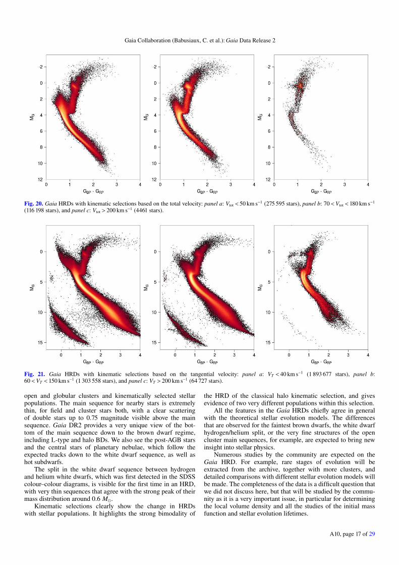
Gaia Collaboration (Babusiaux, C. et al.): Gaia Data Release 2

Fig. 20. Gaia HRDs with kinematic selections based on the total velocity: panel a: Vtot < 50 km s−1 (275 595 stars), panel b: 70<Vtot < 180 km s−1

(116 198 stars), and panel c: Vtot > 200 km s−1 (4461 stars).

Fig. 21. Gaia HRDs with kinematic selections based on the tangential velocity: panel a: VT < 40 km s−1 (1 893 677 stars), panel b:60<VT < 150 km s−1 (1 303 558 stars), and panel c: VT > 200 km s−1 (64 727 stars).

open and globular clusters and kinematically selected stellarpopulations. The main sequence for nearby stars is extremelythin, for field and cluster stars both, with a clear scatteringof double stars up to 0.75 magnitude visible above the mainsequence. Gaia DR2 provides a very unique view of the bot-tom of the main sequence down to the brown dwarf regime,including L-type and halo BDs. We also see the post-AGB starsand the central stars of planetary nebulae, which follow theexpected tracks down to the white dwarf sequence, as well ashot subdwarfs.

The split in the white dwarf sequence between hydrogenand helium white dwarfs, which was first detected in the SDSScolour–colour diagrams, is visible for the first time in an HRD,with very thin sequences that agree with the strong peak of theirmass distribution around 0.6 M⊙.

Kinematic selections clearly show the change in HRDswith stellar populations. It highlights the strong bimodality of

the HRD of the classical halo kinematic selection, and givesevidence of two very different populations within this selection.

All the features in the Gaia HRDs chiefly agree in generalwith the theoretical stellar evolution models. The differencesthat are observed for the faintest brown dwarfs, the white dwarfhydrogen/helium split, or the very fine structures of the opencluster main sequences, for example, are expected to bring newinsight into stellar physics.

Numerous studies by the community are expected on theGaia HRD. For example, rare stages of evolution will beextracted from the archive, together with more clusters, anddetailed comparisons with different stellar evolution models willbe made. The completeness of the data is a difficult question thatwe did not discuss here, but that will be studied by the commu-nity as it is a very important issue, in particular for determiningthe local volume density and all the studies of the initial massfunction and stellar evolution lifetimes.

A10, page 17 of 29

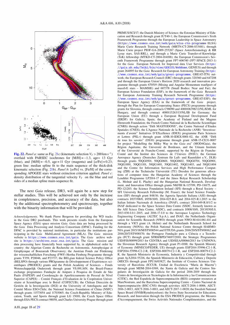
A&A 616, A10 (2018)

Fig. 22. Panel a: same as Fig. 21c (kinematic selection VT > 200 km s−1)overlaid with PARSEC isochrones for [M/H] =−1.3, age= 13 Gyr(blue), and [M/H] =−0.5, age = 11 Gyr (magenta) and [α/Fe] = 0.23;green line: median spline fit to the main sequence of the thick-diskkinematic selection (Fig. 21b). Panel b: [α/Fe] vs. [Fe/H] of the corre-sponding APOGEE stars without extinction criterion applied. Panel c:density distribution of the tangential velocity VT on the blue and redsides of a median spline main-sequence fit.

The next Gaia release, DR3, will again be a new step forstellar studies. This will be achieved not only by the increasein completeness, precision, and accuracy of the data, but alsoby the additional spectrophotometry and spectroscopy, togetherwith the binarity information that will be provided.

Acknowledgements. We thank Pierre Bergeron for providing the WD tracksin the Gaia DR2 passbands. This work presents results from the EuropeanSpace Agency (ESA) space mission Gaia. Gaia data are being processed bythe Gaia Data Processing and Analysis Consortium (DPAC). Funding for theDPAC is provided by national institutions, in particular the institutions par-ticipating in the Gaia MultiLateral Agreement (MLA). The Gaia missionwebsite is https://www.cosmos.esa.int/gaia. The Gaia archive web-site is https://archives.esac.esa.int/gaia. The Gaia mission anddata processing have financially been supported by, in alphabetical order bycountry: the Algerian Centre de Recherche en Astronomie, Astrophysique etGéophysique of Bouzareah Observatory; the Austrian Fonds zur Förderungder wissenschaftlichen Forschung (FWF) Hertha Firnberg Programme throughgrants T359, P20046, and P23737; the BELgian federal Science Policy Office(BELSPO) through various PROgramme de Développement d’Expériences sci-entifiques (PRODEX) grants and the Polish Academy of Sciences – FondsWetenschappelijk Onderzoek through grant VS.091.16N; the Brazil-Franceexchange programmes Fundação de Amparo à Pesquisa do Estado de SãoPaulo (FAPESP) and Coordenação de Aperfeicoamento de Pessoal de NívelSuperior (CAPES) – Comité Français d’Evaluation de la Coopération Univer-sitaire et Scientifique avec le Brésil (COFECUB); the Chilean Dirección deGestión de la Investigación (DGI) at the University of Antofagasta and theComité Mixto ESO-Chile; the National Science Foundation of China (NSFC)through grants 11573054 and 11703065; the Czech-Republic Ministry of Edu-cation, Youth, and Sports through grant LG 15010, the Czech Space Officethrough ESA PECS contract 98058, and Charles University Prague through grant

PRIMUS/SCI/17; the Danish Ministry of Science; the Estonian Ministry of Edu-cation and Research through grant IUT40-1; the European Commission’s SixthFramework Programme through the European Leadership in Space Astrometry(https://www.cosmos.esa.int/web/gaia/elsa-rtn-programme ELSA)Marie Curie Research Training Network (MRTN-CT-2006-033481), throughMarie Curie project PIOF-GA-2009-255267 (Space AsteroSeismology & RRLyrae stars, SAS-RRL), and through a Marie Curie Transfer-of-Knowledge(ToK) fellowship (MTKD-CT-2004-014188); the European Commission’s Sev-enth Framework Programme through grant FP7-606740 (FP7-SPACE-2013-1)for the Gaia European Network for Improved data User Services (https://gaia.ub.edu/Twiki/bin/view/GENIUS/WebHome, GENIUS) and throughgrant 264895 for the Gaia Research for European Astronomy Training (https://www.cosmos.esa.int/web/gaia/great-programme, GREAT-ITN) net-work; the European Research Council (ERC) through grants 320360 and 647208and through the European Union’s Horizon 2020 research and innovation pro-gramme through grants 670519 (Mixing and Angular Momentum tranSport ofmassIvE stars – MAMSIE) and 687378 (Small Bodies: Near and Far); theEuropean Science Foundation (ESF), in the framework of the Gaia Researchfor European Astronomy Training Research Network Programme (https://www.cosmos.esa.int/web/gaia/great-programme, GREAT-ESF); theEuropean Space Agency (ESA) in the framework of the Gaia project,through the Plan for European Cooperating States (PECS) programme throughgrants for Slovenia, through contracts C98090 and 4000106398/12/NL/KML forHungary, and through contract 4000115263/15/NL/IB for Germany; theEuropean Union (EU) through a European Regional Development Fund(ERDF) for Galicia, Spain; the Academy of Finland and the MagnusEhrnrooth Foundation; the French Centre National de la Recherche Scientifique(CNRS) through action “Défi MASTODONS”, the Centre National d’EtudesSpatiales (CNES), the L’Agence Nationale de la Recherche (ANR) “Investisse-ments d’avenir” Initiatives D’EXcellence (IDEX) programme Paris Scienceset Lettres (PSL∗) through grant ANR-10-IDEX-0001-02, the ANR “Défide tous les savoirs” (DS10) programme through grant ANR-15-CE31-0007for project “Modelling the Milky Way in the Gaia era” (MOD4Gaia), theRégion Aquitaine, the Université de Bordeaux, and the Utinam Instituteof the Université de Franche-Comté, supported by the Région de Franche-Comté and the Institut des Sciences de l’Univers (INSU); the GermanAerospace Agency (Deutsches Zentrum für Luft- und Raumfahrt e.V., DLR)through grants 50QG0501, 50QG0601, 50QG0602, 50QG0701, 50QG0901,50QG1001, 50QG1101, 50QG1401, 50QG1402, 50QG1403, and 50QG1404and the Centre for Information Services and High Performance Comput-ing (ZIH) at the Technische Universität (TU) Dresden for generous alloca-tions of computer time; the Hungarian Academy of Sciences through theLendület Programme LP2014-17 and the János Bolyai Research Scholarship(L. Molnár and E. Plachy) and the Hungarian National Research, Develop-ment, and Innovation Office through grants NKFIH K-115709, PD-116175, andPD-121203; the Science Foundation Ireland (SFI) through a Royal Society –SFI University Research Fellowship (M. Fraser); the Israel Science Founda-tion (ISF) through grant 848/16; the Agenzia Spaziale Italiana (ASI) throughcontracts I/037/08/0, I/058/10/0, 2014-025-R.0, and 2014-025-R.1.2015 to theItalian Istituto Nazionale di Astrofisica (INAF), contract 2014-049-R.0/1/2 toINAF dedicated to the Space Science Data Centre (SSDC, formerly known asthe ASI Sciece Data Centre, ASDC), and contracts I/008/10/0, 2013/030/I.0,2013-030-I.0.1-2015, and 2016-17-I.0 to the Aerospace Logistics TechnologyEngineering Company (ALTEC S.p.A.), and INAF; the Netherlands Organi-sation for Scientific Research (NWO) through grant NWO-M-614.061.414 andthrough a VICI grant (A. Helmi) and the Netherlands Research School forAstronomy (NOVA); the Polish National Science Centre through HARMO-NIA grant 2015/18/M/ST9/00544 and ETIUDA grants 2016/20/S/ST9/00162 and2016/20/T/ST9/00170; the Portugese Fundação para a Ciência e a Tecnolo-gia (FCT) through grant SFRH/BPD/74697/2010; the Strategic ProgrammesUID/FIS/00099/2013 for CENTRA and UID/EEA/00066/2013 for UNINOVA;the Slovenian Research Agency through grant P1-0188; the Spanish Ministryof Economy (MINECO/FEDER, UE) through grants ESP2014-55996-C2-1-R,ESP2014-55996-C2-2-R, ESP2016-80079-C2-1-R, and ESP2016-80079-C2-2-R, the Spanish Ministerio de Economía, Industria y Competitividad throughgrant AyA2014-55216, the Spanish Ministerio de Educación, Cultura y Deporte(MECD) through grant FPU16/03827, the Institute of Cosmos Sciences Uni-versity of Barcelona (ICCUB, Unidad de Excelencia “María de Maeztu”)through grant MDM-2014-0369, the Xunta de Galicia and the Centros Sin-gulares de Investigación de Galicia for the period 2016-2019 through theCentro de Investigación en Tecnologías de la Información y las Comunicaciones(CITIC), the Red Española de Supercomputación (RES) computer resources atMareNostrum, and the Barcelona Supercomputing Centre – Centro Nacional deSupercomputación (BSC-CNS) through activities AECT-2016-1-0006, AECT-2016-2-0013, AECT-2016-3-0011, and AECT-2017-1-0020; the Swedish NationalSpace Board (SNSB/Rymdstyrelsen); the Swiss State Secretariat for Education,Research, and Innovation through the ESA PRODEX programme, the Mesuresd’Accompagnement, the Swiss Activités Nationales Complémentaires, and the

A10, page 18 of 29

Gaia Collaboration (Babusiaux, C. et al.): Gaia Data Release 2

Swiss National Science Foundation; the United Kingdom Rutherford AppletonLaboratory, the United Kingdom Science and Technology Facilities Coun-cil (STFC) through grant ST/L006553/1, the United Kingdom Space Agency(UKSA) through grant ST/N000641/1 and ST/N001117/1, as well as a ParticlePhysics and Astronomy Research Council Grant PP/C503703/1. This publicationhas made use of SIMBAD and VizieR, both operated at the Centre de Don-nées astronomiques de Strasbourg (CDS, http://cds.u-strasbg.fr/). Thispublication has made use of data products from the Two Micron All Sky Sur-vey, which is a joint project of the University of Massachusetts and the InfraredProcessing and Analysis Center/California Institute of Technology, funded bythe National Aeronautics and Space Administration and the National ScienceFoundation. This publication has made use of data products from SDSS-III.The Funding for SDSS-III has been provided by the Alfred P. Sloan Foun-dation, the Participating Institutions, the National Science Foundation, andthe U.S. Department of Energy Office of Science. The SDSS-III web site ishttp://www.sdss3.org/. SDSS-III is managed by the Astrophysical ResearchConsortium for the Participating Institutions of the SDSS-III Collaboration.

References

Ahn, C. P., Alexandroff, R., Allende Prieto, C., et al. 2012, ApJS, 203, 21Allard, F., Homeier, D., & Freytag, B. 2012, Phil. Trans. R. Soc. London, Ser. A,

370, 2765Anderson, J., Piotto, G., King, I. R., Bedin, L. R., & Guhathakurta, P. 2009, ApJ,

697, L58Andrae, R., Fouesneau, M., Creevey, O., et al. 2018, A&A, 616, A8 (Gaia 2 SI)Arenou, F., Luri, X., Babusiaux, C., et al. 2018, A&A, 616, A17 (Gaia 2 SI)Baraffe, I., Homeier, D., Allard, F., & Chabrier, G. 2015, A&A, 577, A42Barnes, S. A., Weingrill, J., Fritzewski, D., Strassmeier, K. G., & Platais, I. 2016,

ApJ, 823, 16Barstow, M. A., Bond, H. E., Holberg, J. B., et al. 2005, MNRAS, 362, 1134Bell, C. P. M. 2016, in 19th Cambridge Workshop on Cool Stars, Stellar Systems,

and the Sun (CS19), 102Bensby, T., Feltzing, S., & Oey, M. S. 2014, A&A, 562, A71Bergeron, P., Wesemael, F., Dufour, P., et al. 2011, ApJ, 737, 28Bonaca, A., Conroy, C., Wetzel, A., Hopkins, P. F., & Kereš D. 2017, ApJ, 845,

101Bovy, J. 2016, ApJ, 817, 49Cantat-Gaudin, T., Vallenari, A., Zaggia, S., et al. 2014, A&A, 569, A17Capitanio, L., Lallement, R., Vergely, J. L., Elyajouri, M., & Monreal-Ibero, A.

2017, A&A, 606, A65Carollo, D., Beers, T. C., Lee, Y. S., et al. 2007, Nature, 450, 1020Carrasco, J. M., Catalán, S., Jordi, C., et al. 2014, A&A, 565, A11Carretta, E., Bragaglia, A., Gratton, R. G., et al. 2009, A&A, 505, 117Castelli, F., & Kurucz, R. L. 2003, in Modelling of Stellar Atmospheres, eds.

N. Piskunov, W. W. Weiss, & D. F. Gray, IAU Symp., 210, A20Chen, Y., Girardi, L., Bressan, A., et al. 2014, MNRAS, 444, 2525Christensen-Dalsgaard, J. 2015, MNRAS, 453, 666Clariá, J. J., Piatti, A. E., Lapasset, E., & Parisi, M. C. 2005, Baltic Astron., 14,

301Conrad, C., Scholz, R.-D., Kharchenko, N. V., et al. 2014, A&A, 562, A54Danielski, C., Babusiaux, C., Ruiz-Dern, L., Sartoretti, P., & Arenou, F. 2018,

A&A, 614, A19David, T. J., Conroy, K. E., Hillenbrand, L. A., et al. 2016, AJ, 151, 112de Jong, J. T. A., Yanny, B., Rix, H.-W., et al. 2010, ApJ, 714, 663Denissenkov, P. A., VandenBerg, D. A., Kopacki, G., & Ferguson, J. W. 2017,

ApJ, 849, 159Dotter, A., Sarajedini, A., Anderson, J., et al. 2010, ApJ, 708, 698Dufour, P., Blouin, S., Coutu, S., et al. 2017, in 20th European White Dwarf

Workshop, eds. P.-E. Tremblay, B. Gaensicke, & T. Marsh, ASP Conf. Ser.,509, 3

Evans, D., Riello, M., De Angeli, F., et al. 2018, A&A, 616, A4 (Gaia 2 SI)Faherty, J. K., Burgasser, A. J., Cruz, K. L., et al. 2009, AJ, 137, 1Fitzpatrick, E. L., & Massa, D. 2007, ApJ, 663, 320Ford, A., Jeffries, R. D., & Smalley, B. 2005, MNRAS, 364, 272Gaia Collaboration (Brown, A. G. A., et al.) 2016, A&A, 595, A2Gaia Collaboration (van Leeuwen, F., et al.) 2017, A&A, 601, A19Gaia Collaboration (Brown, A. G. A., et al.) 2018a, A&A, 616, A1 (Gaia 2 SI)Gaia Collaboration (Eyer, L., et al.) 2018b, A&A, submitted (Gaia 2 SI)Gaia Collaboration (Helmi, A., et al.) 2018c, A&A, 616, A12 (Gaia 2 SI)Gaia Collaboration (Katz, D., et al.) 2018d, A&A, 616, A11 (Gaia 2 SI)Gallart, C. 1998, ApJ, 495, L43Girardi, L. 1999, MNRAS, 308, 818Girardi, L. 2016, ARA&A, 54, 95Gliese, W., & Jahreiß, H. 1991, in The Astronomical Data Center CD-ROM:

Selected Astronomical Catalogs, eds. L. E. Brotzmann, & S. E. Gesser(Greenbelt: NASA Goddard Space Flight Center), 1

Gratton, R. G., Lucatello, S., Sollima, A., et al. 2013, A&A, 549, A41Harris, H. C., Liebert, J., Kleinman, S. J., et al. 2003, AJ, 126, 1023Harris, W. E. 1996, AJ, 112, 1487Heber, U. 2009, ARA&A, 47, 211Henry, T. J., & Jao, W.-C. 2015, IAU General Assembly, 22, 2253773Hill, V., Lecureur, A., Gómez, A., et al. 2011, A&A, 534, A80Holberg, J. B., & Bergeron, P. 2006, AJ, 132, 1221Holtzman, J. A., Shetrone, M., Johnson, J. A., et al. 2015, AJ, 150, 148Hurley, J., & Tout, C. A. 1998, MNRAS, 300, 977Jordi, C., Gebran, M., Carrasco, J. M., et al. 2010, A&A, 523, A48Joyce, S. R. G., Barstow, M. A., Casewell, S. L., Holberg, J. B., & Bond,

H. E. 2017, in 20th European White Dwarf Workshop, eds. P.-E. Tremblay,B. Gaensicke, & T. Marsh, ASP Conf. Ser., 509, 389

Juarez, A. J., Cargile, P. A., James, D. J., & Stassun, K. G. 2014, ApJ, 795, 143Kerber, F., Mignani, R. P., Guglielmetti, F., & Wicenec, A. 2003, A&A, 408,

1029Kharchenko, N. V., Piskunov, A. E., Röser, S., Schilbach, E., & Scholz, R.-D.

2005, A&A, 438, 1163Kharchenko, N. V., Piskunov, A. E., Schilbach, E., Roeser, S., & Scholz, R.-D.

2015, VizieR Online Data Catalog: J/A+A/585/A101Kleinman, S. J., Kepler, S. O., Koester, D., et al. 2013, ApJS, 204, 5Kowalski, P. M., & Saumon, D. 2006, ApJ, 651, L137Lallement, R., Welsh, B. Y., Vergely, J. L., Crifo, F., & Sfeir, D. 2003, A&A,

411, 447Lindegren, L., Hernández, J., Bombrun, A. et al. 2018, A&A, 616, A2 (Gaia 2 SI)Liu, F., Yong, D., Asplund, M., Ramírez, I., & Meléndez, J. 2016, MNRAS, 457,

3934Loktin, A. V., & Beshenov, G. V. 2003, Astron. Rep., 47, 6Luri, X., Brown, A. G. A., Sarro, L., et al. 2018, A&A, 616, A9 (Gaia 2 SI)Marigo, P., Girardi, L., Bressan, A., et al. 2017, ApJ, 835, 77Marino, A. F., Milone, A. P., Przybilla, N., et al. 2014, MNRAS, 437, 1609Marrese, P., Marinoni, S., Fabrizio, M., & Altavilla, G. 2018, A&A, submitted

(Gaia 2 SI)Michaud, G., Richard, O., Richer, J., & VandenBerg, D. A. 2004, ApJ, 606, 452Miglio, A., Brogaard, K., & Handberg, R. 2015, IAU General Assembly, 22,

2251619Milone, A. P., Piotto, G., Bedin, L. R., et al. 2012, ApJ, 744, 58Moraux, E., Bouvier, J., Stauffer, J. R., Barrado y Navascués, D., & Cuillandre,

J.-C. 2007, A&A, 471, 499Mucciarelli, A., Dalessandro, E., Massari, D., et al. 2016, ApJ, 824, 73Netopil, M., Paunzen, E., & Carraro, G. 2015, A&A, 582, A19Netopil, M., Paunzen, E., Heiter, U., & Soubiran, C. 2016, A&A, 585, A150Nissen, P. E., & Schuster, W. J. 2010, A&A, 511, L10Parsons, S. G., Gänsicke, B. T., Marsh, T. R., et al. 2017, MNRAS, 470, 4473Pasetto, S., Chiosi, C., Chiosi, E., Cropper, M., & Weiss, A. 2016, MNRAS,

459, 3182Perryman, M. A. C., Lindegren, L., Kovalevsky, J., et al. 1995, A&A, 304, 69Posti, L., Helmi, A., Veljanoski, J., & Breddels, M. 2018, A&A, 615, A70Powalka, M., Lançon, A., Puzia, T. H., et al. 2017, ApJ, 844, 104Provencal, J. L., Shipman, H. L., Høg, E., & Thejll, P. 1998, ApJ, 494, 759Ruiz-Dern, L., Babusiaux, C., Arenou, F., Turon, C., & Lallement, R. 2018,

A&A, 609, A116Salaris, M., Chieffi, A., & Straniero, O. 1993, ApJ, 414, 580Sartoretti, P., Katz, D., Cropper, M., et al. 2018, A&A, 616, A6 (Gaia 2 SI)Saumon, D., & Marley, M. S. 2008, ApJ, 689, 1327Schlegel, D. J., Finkbeiner, D. P., & Davis, M. 1998, ApJ, 500, 525Skrutskie, M. F., Cutri, R. M., Stiening, R., et al. 2006, AJ, 131, 1163Smart, R. L., Marocco, F., Caballero, J. A., et al. 2017, MNRAS, 469, 401Stello, D., Vanderburg, A., Casagrande, L., et al. 2016, ApJ, 832, 133Szczerba, R., Siódmiak, N., Stasinska, G., & Borkowski, J. 2007, A&A, 469, 799Taylor, B. J. 2007, AJ, 133, 370Tremblay, P.-E., Ludwig, H.-G., Steffen, M., Bergeron, P., & Freytag, B. 2011,

A&A, 531, L19Tremblay, P.-E., Gentile-Fusillo, N., Raddi, R., et al. 2017, MNRAS, 465, 2849Valcarce, A. A. R., Catelan, M., Alonso-García, J., Contreras Ramos, R., &

Alves, S. 2016, A&A, 589, A126van Leeuwen, F. 2009, A&A, 497, 209Weiss, A., & Heners, N. 2013, Eur. Phys. J. Web Conf., 43, 01002Zinn, R. 1985, ApJ, 293, 424

1 Université Grenoble Alpes, CNRS, IPAG, 38000 Grenoble, France2 GEPI, Observatoire de Paris, Université PSL, CNRS, 5 Place Jules

Janssen, 92190 Meudon, France3 Institute of Astronomy, University of Cambridge, Madingley Road,

Cambridge CB3 0HA, UK

A10, page 19 of 29

A&A 616, A10 (2018)

4 Leicester Institute of Space and Earth Observation and Depart-ment of Physics and Astronomy, University of Leicester, UniversityRoad, Leicester LE1 7RH, UK

5 Institut de Ciències del Cosmos, Universitat de Barcelona (IEEC-UB), Martí i Franquès 1, 08028 Barcelona, Spain

6 INAF – Osservatorio astronomico di Padova, Vicolo Osservatorio5, 35122 Padova, Italy

7 SISSA – Scuola Internazionale Superiore di Studi Avanzati, viaBonomea 265, 34136 Trieste, Italy

8 Leiden Observatory, Leiden University, Niels Bohrweg 2, 2333 CALeiden, The Netherlands

9 Science Support Office, Directorate of Science, European SpaceResearch and Technology Centre (ESA/ESTEC), Keplerlaan 1,2201 AZ Noordwijk, The Netherlands

10 Max Planck Institute for Astronomy, Königstuhl 17, 69117 Heidel-berg, Germany

11 Astronomisches Rechen-Institut, Zentrum für Astronomie derUniversität Heidelberg, Mönchhofstr. 12-14, 69120 Heidelberg,Germany

12 Department of Astronomy, University of Geneva, Chemin desMaillettes 51, 1290 Versoix, Switzerland

13 Mission Operations Division, Operations Department, Directorateof Science, European Space Research and Technology Centre(ESA/ESTEC), Keplerlaan 1, 2201 AZ Noordwijk, The Netherlands

14 Lohrmann Observatory, Technische Universität Dresden, Momm-senstraße 13, 01062 Dresden, Germany

15 European Space Astronomy Centre (ESA/ESAC), Camino bajo delCastillo s/n, Urbanización Villafranca del Castillo, Villanueva de laCañada, 28692 Madrid, Spain

16 Lund Observatory, Department of Astronomy and TheoreticalPhysics, Lund University, Box 43, 22100 Lund, Sweden

17 Université Côte d’Azur, Observatoire de la Côte d’Azur, CNRS,Laboratoire Lagrange, Bd de l’Observatoire, CS 34229, 06304 NiceCedex 4, France

18 CNES Centre Spatial de Toulouse, 18 avenue Edouard Belin, 31401Toulouse Cedex 9, France

19 Institut d’Astronomie et d’Astrophysique, Université Libre deBruxelles CP 226, Boulevard du Triomphe, 1050 Bruxelles,Belgium

20 F.R.S.-FNRS, Rue d’Egmont 5, 1000 Bruxelles, Belgium21 INAF – Osservatorio Astrofisico di Arcetri, Largo Enrico Fermi 5,

50125 Firenze, Italy22 Telespazio Vega UK Ltd for ESA/ESAC, Camino bajo del Castillo

s/n, Urbanización Villafranca del Castillo, Villanueva de la Cañada,28692 Madrid, Spain

23 Laboratoire d’astrophysique de Bordeaux, Univ. Bordeaux, CNRS,B18N, allée Geoffroy Saint-Hilaire, 33615 Pessac, France

24 Mullard Space Science Laboratory, University College London,Holmbury St Mary, Dorking, Surrey RH5 6NT, UK

25 INAF – Osservatorio Astrofisico di Torino, via Osservatorio 20,10025 Pino Torinese, Italy

26 INAF – Osservatorio di Astrofisica e Scienza dello Spazio diBologna, via Piero Gobetti 93/3, 40129 Bologna, Italy

27 Serco Gestión de Negocios for ESA/ESAC, Camino bajo delCastillo s/n, Urbanización Villafranca del Castillo, Villanueva dela Cañada, 28692 Madrid, Spain

28 ALTEC SpA, Corso Marche 79, 10146 Torino, Italy29 Department of Astronomy, University of Geneva, Chemin d’Ecogia

16, 1290 Versoix, Switzerland30 Gaia DPAC Project Office, ESAC, Camino bajo del Castillo s/n,

Urbanización Villafranca del Castillo, Villanueva de la Cañada,28692 Madrid, Spain

31 SYRTE, Observatoire de Paris, Université PSL, CNRS, Sor-bonne Université, LNE, 61 avenue de l’Observatoire 75014 Paris,France

32 National Observatory of Athens, I. Metaxa and Vas. Pavlou, PalaiaPenteli, 15236 Athens, Greece

33 IMCCE, Observatoire de Paris, Université PSL, CNRS, SorbonneUniversité, Univ. Lille, 77 av. Denfert-Rochereau, 75014 Paris,France

34 Royal Observatory of Belgium, Ringlaan 3, 1180 Brussels,Belgium

35 Institute for Astronomy, University of Edinburgh, Royal Observa-tory, Blackford Hill, Edinburgh EH9 3HJ, UK

36 Instituut voor Sterrenkunde, KU Leuven, Celestijnenlaan 200D,3001 Leuven, Belgium

37 Institut d’Astrophysique et de Géophysique, Université de Liège,19c Allée du 6 Août, B-4000 Liège, Belgium

38 ATG Europe for ESA/ESAC, Camino bajo del Castillo s/n, Urban-ización Villafranca del Castillo, Villanueva de la Cañada, 28692Madrid, Spain

39 Área de Lenguajes y Sistemas Informáticos, Universidad Pablo deOlavide, Ctra. de Utrera, km 1. 41013 Sevilla, Spain

40 ETSE Telecomunicación, Universidade de Vigo, Campus Lagoas-Marcosende, 36310 Vigo, Spain

41 Large Synoptic Survey Telescope, 950 N. Cherry Avenue, Tucson,AZ 85719, USA

42 Observatoire Astronomique de Strasbourg, Université de Stras-bourg, CNRS, UMR 7550, 11 rue de l’Université, 67000 Stras-bourg, France

43 Kavli Institute for Cosmology, University of Cambridge, MadingleyRoad, Cambride CB3 0HA, UK

44 Aurora Technology for ESA/ESAC, Camino bajo del Castillo s/n,Urbanización Villafranca del Castillo, Villanueva de la Cañada,28692 Madrid, Spain

45 Laboratoire Univers et Particules de Montpellier, Université Mont-pellier, Place Eugène Bataillon, CC72, 34095 Montpellier Cedex05, France

46 Department of Physics and Astronomy, Division of Astronomyand Space Physics, Uppsala University, Box 516, 75120 Uppsala,Sweden

47 CENTRA, Universidade de Lisboa, FCUL, Campo Grande, Edif.C8, 1749-016 Lisboa, Portugal

48 Università di Catania, Dipartimento di Fisica e Astronomia,Sezione Astrofisica, Via S. Sofia 78, 95123 Catania, Italy

49 INAF – Osservatorio Astrofisico di Catania, via S. Sofia 78, 95123Catania, Italy

50 Department of Astrophysics, University of Vienna, Türkenschanzs-traße 17, A1180 Vienna, Austria

51 CITIC – Department of Computer Science, University of A Coruña,Campus de Elviña s/n, 15071, A Coruña, Spain

52 CITIC – Astronomy and Astrophysics, University of A Coruña,Campus de Elviña s/n, 15071, A Coruña, Spain

53 INAF – Osservatorio Astronomico di Roma, Via di Frascati 33,00078 Monte Porzio Catone, Italy

54 Space Science Data Center – ASI, Via del Politecnico SNC, 00133Roma, Italy

55 Department of Physics, University of Helsinki, P.O. Box 64, 00014Helsinki, Finland

56 Finnish Geospatial Research Institute FGI, Geodeetinrinne 2,02430 Masala, Finland

57 Isdefe for ESA/ESAC, Camino bajo del Castillo s/n, UrbanizaciónVillafranca del Castillo, Villanueva de la Cañada, 28692 Madrid,Spain

58 Institut UTINAM UMR6213, CNRS, OSU THETA Franche-Comté Bourgogne, Université Bourgogne Franche-Comté, 25000Besançon, France

59 STFC, Rutherford Appleton Laboratory, Harwell, Didcot OX110QX, UK

60 Departamento de Inteligencia Artificial, UNED, c/ Juan del Rosal16, 28040 Madrid, Spain

61 Elecnor Deimos Space for ESA/ESAC, Camino bajo del Castillos/n, Urbanización Villafranca del Castillo, Villanueva de la Cañada,28692 Madrid, Spain

62 Thales Services for CNES Centre Spatial de Toulouse, 18 avenueEdouard Belin, 31401 Toulouse Cedex 9, France

63 Department of Astrophysics/IMAPP, Radboud University, PO Box9010, 6500 GL Nijmegen, The Netherlands

64 European Southern Observatory, Karl-Schwarzschild-Str. 2, 85748Garching, Germany

A10, page 20 of 29

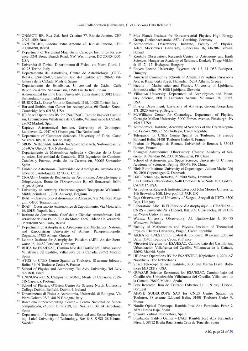
Gaia Collaboration (Babusiaux, C. et al.): Gaia Data Release 2

65 ON/MCTI-BR, Rua Gal. José Cristino 77, Rio de Janeiro, CEP20921-400, Brazil

66 OV/UFRJ-BR, Ladeira Pedro Antônio 43, Rio de Janeiro, CEP20080-090, Brazil

67 Department of Terrestrial Magnetism, Carnegie Institution for Sci-ence, 5241 Broad Branch Road, NW, Washington, DC 20015-1305,USA

68 Università di Torino, Dipartimento di Fisica, via Pietro Giuria 1,10125 Torino, Italy

69 Departamento de Astrofísica, Centro de Astrobiología (CSIC-INTA), ESA-ESAC, Camino Bajo del Castillo s/n, 28692 Vil-lanueva de la Cañada, Madrid, Spain

70 Departamento de Estadística, Universidad de Cádiz, CalleRepública Árabe Saharawi s/n, 11510 Puerto Real, Spain

71 Astronomical Institute Bern University, Sidlerstrasse 5, 3012 Bern,Switzerland (present address)

72 EURIX S.r.l., Corso Vittorio Emanuele II 61, 10128 Torino, Italy73 Harvard-Smithsonian Center for Astrophysics, 60 Garden Street,

Cambridge MA 02138, USA74 HE Space Operations BV for ESA/ESAC, Camino bajo del Castillo

s/n, Urbanización Villafranca del Castillo, Villanueva de la Cañada,28692 Madrid, Spain

75 Kapteyn Astronomical Institute, University of Groningen,Landleven 12, 9747 AD Groningen, The Netherlands

76 Department of Computer Sciences, University of Turin, CorsoSvizzera 185, 10149 Torino, Italy

77 SRON, Netherlands Institute for Space Research, Sorbonnelaan 2,3584CA Utrecht, The Netherlands

78 Departamento de Matemática Aplicada y Ciencias de la Com-putación, Universidad de Cantabria, ETS Ingenieros de Caminos,Canales y Puertos, Avda. de los Castros s/n, 39005 Santander,Spain

79 Unidad de Astronomía, Universidad de Antofagasta, Avenida Ang-amos 601, Antofagasta 1270300, Chile

80 CRAAG – Centre de Recherche en Astronomie, Astrophysique etGéophysique, Route de l’Observatoire Bp 63 Bouzareah 16340Alger, Algeria

81 University of Antwerp, Onderzoeksgroep Toegepaste Wiskunde,Middelheimlaan 1, 2020 Antwerp, Belgium

82 INAF – Osservatorio Astronomico d’Abruzzo, Via Mentore Mag-gini, 64100 Teramo, Italy

83 INAF – Osservatorio Astronomico di Capodimonte, Via Moiariello16, 80131 Napoli, Italy

84 Instituto de Astronomia, Geofìsica e Ciências Atmosféricas, Uni-versidade de São Paulo, Rua do Matão 1226, Cidade Universitaria,05508-900 São Paulo, Brazil

85 Department of Astrophysics, Astronomy and Mechanics, Nationaland Kapodistrian University of Athens, Panepistimiopolis,Zografos, 15783 Athens, Greece

86 Leibniz Institute for Astrophysics Potsdam (AIP), An der Stern-warte 16, 14482 Potsdam, Germany

87 RHEA for ESA/ESAC, Camino bajo del Castillo s/n, UrbanizaciónVillafranca del Castillo, Villanueva de la Cañada, 28692 Madrid,Spain

88 ATOS for CNES Centre Spatial de Toulouse, 18 avenue EdouardBelin, 31401 Toulouse Cedex 9, France

89 School of Physics and Astronomy, Tel Aviv University, Tel Aviv6997801, Israel

90 UNINOVA – CTS, Campus FCT-UNL, Monte da Caparica, 2829-516 Caparica, Portugal

91 School of Physics, O’Brien Centre for Science North, UniversityCollege Dublin, Belfield, Dublin 4, Ireland

92 Dipartimento di Fisica e Astronomia, Università di Bologna, ViaPiero Gobetti 93/2, 40129 Bologna, Italy

93 Barcelona Supercomputing Center – Centro Nacional de Super-computación, c/ Jordi Girona 29, Ed. Nexus II, 08034 Barcelona,Spain

94 Department of Computer Science, Electrical and Space Engineer-ing, Luleå University of Technology, Box 848, S-981 28 Kiruna,Sweden

95 Max Planck Institute for Extraterrestrial Physics, High EnergyGroup, Gießenbachstraße, 85741 Garching, Germany

96 Astronomical Observatory Institute, Faculty of Physics,Adam Mickiewicz University, Słoneczna 36, 60-286 Poznan,Poland

97 Konkoly Observatory, Research Centre for Astronomy and EarthSciences, Hungarian Academy of Sciences, Konkoly Thege Miklósút 15-17, 1121 Budapest, Hungary

98 Eötvös Loránd University, Egyetem tér 1-3, H-1053 Budapest,Hungary

99 American Community Schools of Athens, 129 Aghias ParaskevisAve. & Kazantzaki Street, Halandri, 15234 Athens, Greece

100 Faculty of Mathematics and Physics, University of Ljubljana,Jadranska ulica 19, 1000 Ljubljana, Slovenia

101 Villanova University, Department of Astrophysics and Plane-tary Science, 800 E Lancaster Avenue, Villanova PA 19085,USA

102 Physics Department, University of Antwerp, Groenenborgerlaan171, 2020 Antwerp, Belgium

103 McWilliams Center for Cosmology, Department of Physics,Carnegie Mellon University, 5000 Forbes Avenue, Pittsburgh, PA15213, USA

104 Astronomical Institute, Academy of Sciences of the Czech Repub-lic, Fricova 298, 25165 Ondrejov, Czech Republic

105 Telespazio for CNES Centre Spatial de Toulouse, 18 avenueEdouard Belin, 31401 Toulouse Cedex 9, France

106 Institut de Physique de Rennes, Université de Rennes 1, 35042Rennes, France

107 Shanghai Astronomical Observatory, Chinese Academy of Sci-ences, 80 Nandan Rd, 200030 Shanghai, PR China

108 School of Astronomy and Space Science, University of ChineseAcademy of Sciences, Beijing 100049, PR China

109 Niels Bohr Institute, University of Copenhagen, Juliane Maries Vej30, 2100 Copenhagen Ø, Denmark

110 DXC Technology, Retortvej 8, 2500 Valby, Denmark111 Las Cumbres Observatory, 6740 Cortona Drive Suite 102, Goleta,

CA 93117, USA112 Astrophysics Research Institute, Liverpool John Moores University,

146 Brownlow Hill, Liverpool L3 5RF, UK113 Baja Observatory of University of Szeged, Szegedi út III/70, 6500

Baja, Hungary114 Laboratoire AIM, IRFU/Service d’Astrophysique – CEA/DSM –

CNRS – Université Paris Diderot, Bât. 709, CEA-Saclay, 91191 Gif-sur-Yvette Cedex, France

115 Warsaw University Observatory, Al. Ujazdowskie 4, 00-478Warszawa, Poland

116 Faculty of Mathematics and Physics, Institute of TheoreticalPhysics, Charles University, Prague, Czech Republic

117 AKKA for CNES Centre Spatial de Toulouse, 18 avenue EdouardBelin, 31401 Toulouse Cedex 9, France

118 Vitrociset Belgium for ESA/ESAC, Camino bajo del Castillo s/n,Urbanización Villafranca del Castillo, Villanueva de la Cañada,28692 Madrid, Spain

119 HE Space Operations BV for ESA/ESTEC, Keplerlaan 1, 2201 AZNoordwijk, The Netherlands

120 Space Telescope Science Institute, 3700 San Martin Drive, Balti-more MD 21218, USA

121 QUASAR Science Resources for ESA/ESAC, Camino bajo delCastillo s/n, Urbanización Villafranca del Castillo, Villanueva dela Cañada, 28692 Madrid, Spain

122 Fork Research, Rua do Cruzado Osberno, Lt. 1, 9 esq., Lisboa,Portugal

123 APAVE SUDEUROPE SAS for CNES Centre Spatial deToulouse, 18 avenue Edouard Belin, 31401 Toulouse Cedex 9,France

124 Nordic Optical Telescope, Rambla José Ana Fernández Pérez 7,38711 Breña Baja, Spain

125 Spanish Virtual Observatory, Spain126 Fundación Galileo Galilei – INAF, Rambla José Ana Fernández

Pérez 7, 38712 Breña Baja, Santa Cruz de Tenerife, Spain

A10, page 21 of 29

A&A 616, A10 (2018)

127 INSA for ESA/ESAC, Camino bajo del Castillo s/n, UrbanizaciónVillafranca del Castillo, Villanueva de la Cañada, 28692 Madrid,Spain

128 Departamento de Arquitectura de Computadores y Automática,Facultad de Informática, Universidad Complutense de Madrid, C/Prof. José García Santesmases s/n, 28040 Madrid, Spain

129 H H Wills Physics Laboratory, University of Bristol, TyndallAvenue, Bristol BS8 1TL, UK

130 Institut d’Estudis Espacials de Catalunya (IEEC), Gran Capita 2-4,08034 Barcelona, Spain

131 Applied Physics Department, Universidade de Vigo, 36310 Vigo,Spain

132 Stellar Astrophysics Centre, Aarhus University, Department ofPhysics and Astronomy, 120 Ny Munkegade, Building 1520, DK-8000 Aarhus C, Denmark

133 Argelander-Institut für Astronomie, Universität Bonn, Auf demHügel 71, 53121 Bonn, Germany

134 Research School of Astronomy and Astrophysics, AustralianNational University, Canberra, ACT 2611 Australia

135 Sorbonne Universités, UPMC Univ. Paris 6 et CNRS, UMR 7095,Institut d’Astrophysique de Paris, 98 bis bd. Arago, 75014 Paris,France

136 Department of Geosciences, Tel Aviv University, Tel Aviv 6997801,Israel

A10, page 22 of 29

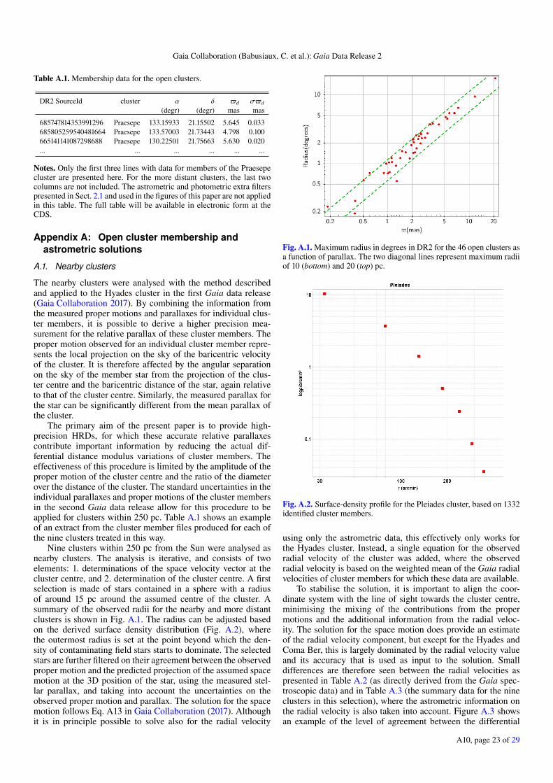
Gaia Collaboration (Babusiaux, C. et al.): Gaia Data Release 2

Table A.1. Membership data for the open clusters.

DR2 SourceId cluster α δ d σd

(degr) (degr) mas mas

685747814353991296 Praesepe 133.15933 21.15502 5.645 0.033685805259540481664 Praesepe 133.57003 21.73443 4.798 0.100665141141087298688 Praesepe 130.22501 21.75663 5.630 0.020... ... ... ... ... ...

Notes. Only the first three lines with data for members of the Praesepecluster are presented here. For the more distant clusters, the last twocolumns are not included. The astrometric and photometric extra filterspresented in Sect. 2.1 and used in the figures of this paper are not appliedin this table. The full table will be available in electronic form at theCDS.

Appendix A: Open cluster membership and

astrometric solutions

A.1. Nearby clusters

The nearby clusters were analysed with the method describedand applied to the Hyades cluster in the first Gaia data release(Gaia Collaboration 2017). By combining the information fromthe measured proper motions and parallaxes for individual clus-ter members, it is possible to derive a higher precision mea-surement for the relative parallax of these cluster members. Theproper motion observed for an individual cluster member repre-sents the local projection on the sky of the baricentric velocityof the cluster. It is therefore affected by the angular separationon the sky of the member star from the projection of the clus-ter centre and the baricentric distance of the star, again relativeto that of the cluster centre. Similarly, the measured parallax forthe star can be significantly different from the mean parallax ofthe cluster.

The primary aim of the present paper is to provide high-precision HRDs, for which these accurate relative parallaxescontribute important information by reducing the actual dif-ferential distance modulus variations of cluster members. Theeffectiveness of this procedure is limited by the amplitude of theproper motion of the cluster centre and the ratio of the diameterover the distance of the cluster. The standard uncertainties in theindividual parallaxes and proper motions of the cluster membersin the second Gaia data release allow for this procedure to beapplied for clusters within 250 pc. Table A.1 shows an exampleof an extract from the cluster member files produced for each ofthe nine clusters treated in this way.

Nine clusters within 250 pc from the Sun were analysed asnearby clusters. The analysis is iterative, and consists of twoelements: 1. determinations of the space velocity vector at thecluster centre, and 2. determination of the cluster centre. A firstselection is made of stars contained in a sphere with a radiusof around 15 pc around the assumed centre of the cluster. Asummary of the observed radii for the nearby and more distantclusters is shown in Fig. A.1. The radius can be adjusted basedon the derived surface density distribution (Fig. A.2), wherethe outermost radius is set at the point beyond which the den-sity of contaminating field stars starts to dominate. The selectedstars are further filtered on their agreement between the observedproper motion and the predicted projection of the assumed spacemotion at the 3D position of the star, using the measured stel-lar parallax, and taking into account the uncertainties on theobserved proper motion and parallax. The solution for the spacemotion follows Eq. A13 in Gaia Collaboration (2017). Althoughit is in principle possible to solve also for the radial velocity

Fig. A.1. Maximum radius in degrees in DR2 for the 46 open clusters asa function of parallax. The two diagonal lines represent maximum radiiof 10 (bottom) and 20 (top) pc.

Fig. A.2. Surface-density profile for the Pleiades cluster, based on 1332identified cluster members.

using only the astrometric data, this effectively only works forthe Hyades cluster. Instead, a single equation for the observedradial velocity of the cluster was added, where the observedradial velocity is based on the weighted mean of the Gaia radialvelocities of cluster members for which these data are available.

To stabilise the solution, it is important to align the coor-dinate system with the line of sight towards the cluster centre,minimising the mixing of the contributions from the propermotions and the additional information from the radial veloc-ity. The solution for the space motion does provide an estimateof the radial velocity component, but except for the Hyades andComa Ber, this is largely dominated by the radial velocity valueand its accuracy that is used as input to the solution. Smalldifferences are therefore seen between the radial velocities aspresented in Table A.2 (as directly derived from the Gaia spec-troscopic data) and in Table A.3 (the summary data for the nineclusters in this selection), where the astrometric information onthe radial velocity is also taken into account. Figure A.3 showsan example of the level of agreement between the differential

A10, page 23 of 29

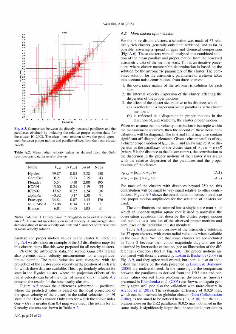
A&A 616, A10 (2018)

Fig. A.3. Comparison between the directly measured parallaxes and theparallaxes obtained by including the relative proper motion data, forthe cluster IC 2602. The clear linear relation shows the good agree-ment between proper motion and parallax offsets from the mean clustervalues.

Table A.2. Mean radial velocity values as derived from the Gaiaspectroscopic data for nearby clusters.

Name Vrad σ(Vrad) uwsd Nobs

Hyades 39.87 0.05 2.28 150ComaBer 0.21 0.13 2.15 43Pleiades 5.54 0.10 2.00 195IC2391 15.00 0.24 1.19 35IC2602 17.62 0.22 1.24 36alphaPer −0.32 0.17 1.38 71Praesepe 34.84 0.07 1.45 176NGC2451A 23.08 0.34 1.32 31Blanco1 6.01 0.15 1.03 51

Notes. Columns: 1. Cluster name; 2: weighted-mean radial velocity inkm s−1; 3. standard uncertainty on radial velocity; 4. unit-weight stan-dard deviation of mean velocity solution; and 5. number of observationsin mean velocity solution.

parallax and proper motion values in the cluster IC 2602. InFig. A.4 we also show an example of the 3D distribution maps forthis cluster; maps like this were prepared for all nearby clusters.

Next to the astrometric data, the second Gaia data releasealso presents radial velocity measurements for a magnitude-limited sample. The radial velocities were compared with theprojection of the cluster space velocity at the position of each starfor which these data are available. This is particularly relevant forstars in the Hyades cluster, where the projection effects of theradial velocity can be of the order of several km s−1. Table A.2presents the results for the nine nearby clusters.

Figure A.5 shows the differences (observed − predicted,where the predicted value is based on the local projection ofthe space velocity of the cluster) in the radial velocities for 191stars in the Hyades cluster. Only stars for which the colour indexGBP −GRP is greater than 0.4 mag were used. The results for all9 nearby clusters are shown in Table A.2.

A.2. More distant open clusters

For the more distant clusters, a selection was made of 37 rela-tively rich clusters, generally only little reddened, and as far aspossible, covering a spread in ages and chemical composition(Fig. A.6). These clusters were all analysed in a combined solu-tion of the mean parallax and proper motion from the observedastrometric data of the member stars. This is an iterative proce-dure, where cluster membership determination is based on thesolution for the astrometric parameters of the cluster. The com-bined solution for the astrometric parameters of a cluster takesinto account noise contributions from three sources:

1. the covariance matrix of the astrometric solution for eachstar;

2. the internal velocity dispersion of the cluster, affecting thedispersion of the proper motions;

3. the effect of the cluster size relative to its distance, which(a) is reflected in a dispersion on the parallaxes of the cluster

members;(b) is reflected in a dispersion in proper motions in the

direction of, and scaled by, the cluster proper motion.

When we assume that the velocity distribution is isotropic withinthe measurement accuracy, then the second of these noise con-tributions will be diagonal. The first and third may also containsignificant off-diagonal elements. Given a cluster parallax ofc,a cluster proper motion of (µα,c, µδ,c), and an average relative dis-persion in the parallaxes of the cluster stars of σ/ = σR/R(where R is the distance to the cluster centre), the contribution tothe dispersion in the proper motions of the cluster stars scaleswith the relative dispersion of the parallaxes and the propermotions of the cluster:

σµα,s = |µα,c| × σ/ (A.1)

σµδ,s = |µδ,c| × σ/. (A.2)

For most of the clusters with distances beyond 250 pc, thiscontribution will be small to very small relative to other contri-butions. Figure A.7 shows the overall relation between parallaxeand proper motion amplitudes for the selection of clusters weused.

The contributions are summed into a single noise matrix, ofwhich an upper-triangular square root is used to normalise theobservation equations that describe the cluster proper motionand parallax as a function of the observed proper motions andparallaxes of the individual cluster members.

Table A.4 presents an overview of the astrometric solutionsfor 37 open clusters, with mean radial velocities when availablein the Gaia data. We note that some clusters are not includedin Table 2 because their colour-magnitude diagrams are toodisturbed by interstellar extinction (see an illustration of the dif-ferential extinction effect in Fig. A.8). The proper motions arecompared with those presented by Loktin & Beshenov (2003) inFig. A.9, and they agree well overall, but there is also an indi-cation that errors on the data presented in Loktin & Beshenov(2003) are underestimated. In the same figure the comparisonbetween the parallaxes as derived from the DR2 data and par-allax values derived from photometric distances as (mostly)presented in Kharchenko et al. (2005) are shown, and again gen-erally agree well (see also the validation with more clusters inArenou et al. 2018). The systematic difference of 0.029 mas,which can be observed for globular clusters (Gaia Collaboration2018c), is too small to be noticed here (Fig. A.10), but the cali-bration noise on the DR2 parallaxes (0.025 mas), obtained in thesame study, is significantly larger than the standard uncertainties

A10, page 24 of 29

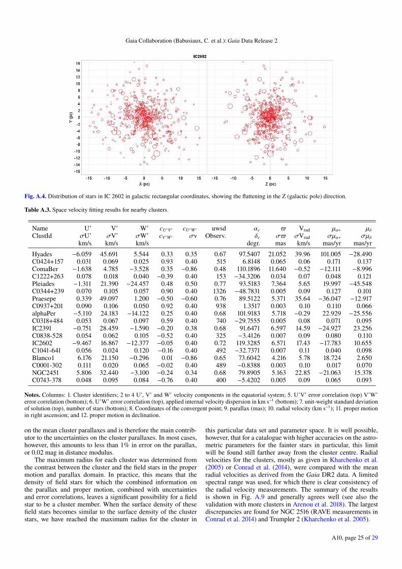
Gaia Collaboration (Babusiaux, C. et al.): Gaia Data Release 2

Fig. A.4. Distribution of stars in IC 2602 in galactic rectangular coordinates, showing the flattening in the Z (galactic pole) direction.

Table A.3. Space velocity fitting results for nearby clusters.

Name U’ V’ W’ cU′V ′ cU′W′ uwsd αc Vrad µα∗ µδClustId σU’ σV’ σW’ cV ′W′ σv Observ. δc σ σVrad σµα∗ σµδ

km/s km/s km/s degr. mas km/s mas/yr mas/yr

Hyades −6.059 45.691 5.544 0.33 0.35 0.67 97.5407 21.052 39.96 101.005 −28.490C0424+157 0.031 0.069 0.025 0.93 0.40 515 6.8148 0.065 0.06 0.171 0.137ComaBer −1.638 4.785 −3.528 0.35 −0.86 0.48 110.1896 11.640 −0.52 −12.111 −8.996C1222+263 0.078 0.018 0.040 −0.39 0.40 153 −34.3206 0.034 0.07 0.048 0.121Pleiades −1.311 21.390 −24.457 0.48 0.50 0.77 93.5183 7.364 5.65 19.997 −45.548C0344+239 0.070 0.105 0.057 0.90 0.40 1326 −48.7831 0.005 0.09 0.127 0.101Praesepe 0.339 49.097 1.200 −0.50 −0.60 0.76 89.5122 5.371 35.64 −36.047 −12.917C0937+201 0.090 0.106 0.050 0.92 0.40 938 1.3517 0.003 0.10 0.110 0.066alphaPer −5.110 24.183 −14.122 0.25 0.40 0.68 101.9183 5.718 −0.29 22.929 −25.556C0318+484 0.053 0.067 0.097 0.59 0.40 740 −29.7555 0.005 0.08 0.071 0.095IC2391 −0.751 28.459 −1.590 −0.20 0.38 0.68 91.6471 6.597 14.59 −24.927 23.256C0838-528 0.054 0.062 0.105 −0.52 0.40 325 −3.4126 0.007 0.09 0.080 0.110IC2602 −9.467 16.867 −12.377 −0.05 0.40 0.72 119.3285 6.571 17.43 −17.783 10.655C1041-641 0.056 0.024 0.120 −0.16 0.40 492 −32.7371 0.007 0.11 0.040 0.098Blanco1 6.176 21.150 −0.296 0.01 −0.86 0.65 73.6042 4.216 5.78 18.724 2.650C0001-302 0.111 0.020 0.065 −0.02 0.40 489 −0.8388 0.003 0.10 0.017 0.070NGC2451 5.806 32.440 −3.100 −0.24 0.34 0.68 79.8905 5.163 22.85 −21.063 15.378C0743-378 0.048 0.095 0.084 −0.76 0.40 400 −5.4202 0.005 0.09 0.065 0.093

Notes. Columns: 1. Cluster identifiers; 2 to 4 U’, V’ and W’ velocity components in the equatorial system; 5. U’V’ error correlation (top) V’W’error correlation (bottom); 6. U’W’ error correlation (top), applied internal velocity dispersion in km s−1 (bottom); 7. unit-weight standard deviationof solution (top), number of stars (bottom); 8. Coordinates of the convergent point; 9. parallax (mas); 10. radial velocity (km s−1); 11. proper motionin right ascension; and 12. proper motion in declination.

on the mean cluster parallaxes and is therefore the main contrib-utor to the uncertainties on the cluster parallaxes. In most cases,however, this amounts to less than 1% in error on the parallax,or 0.02 mag in distance modulus.

The maximum radius for each cluster was determined fromthe contrast between the cluster and the field stars in the propermotion and parallax domain. In practice, this means that thedensity of field stars for which the combined information onthe parallax and proper motion, combined with uncertaintiesand error correlations, leaves a significant possibility for a fieldstar to be a cluster member. When the surface density of thesefield stars becomes similar to the surface density of the clusterstars, we have reached the maximum radius for the cluster in

this particular data set and parameter space. It is well possible,however, that for a catalogue with higher accuracies on the astro-metric parameters for the fainter stars in particular, this limitwill be found still farther away from the cluster centre. Radialvelocities for the clusters, mostly as given in Kharchenko et al.(2005) or Conrad et al. (2014), were compared with the meanradial velocities as derived from the Gaia DR2 data. A limitedspectral range was used, for which there is clear consistency ofthe radial velocity measurements. The summary of the resultsis shown in Fig. A.9 and generally agrees well (see also thevalidation with more clusters in Arenou et al. 2018). The largestdiscrepancies are found for NGC 2516 (RAVE measurements inConrad et al. 2014) and Trumpler 2 (Kharchenko et al. 2005).

A10, page 25 of 29

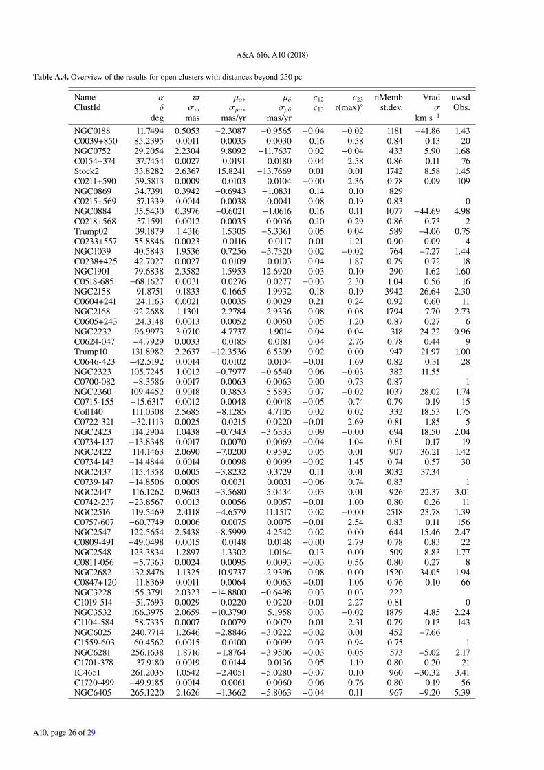
A&A 616, A10 (2018)

Table A.4. Overview of the results for open clusters with distances beyond 250 pc

Name α µα∗ µδ c12 c23 nMemb Vrad uwsdClustId δ σ σµα∗ σµδ c13 r(max)◦ st.dev. σ Obs.

deg mas mas/yr mas/yr km s−1

NGC0188 11.7494 0.5053 −2.3087 −0.9565 −0.04 −0.02 1181 −41.86 1.43C0039+850 85.2395 0.0011 0.0035 0.0030 0.16 0.58 0.84 0.13 20NGC0752 29.2054 2.2304 9.8092 −11.7637 0.02 −0.04 433 5.90 1.68C0154+374 37.7454 0.0027 0.0191 0.0180 0.04 2.58 0.86 0.11 76Stock2 33.8282 2.6367 15.8241 −13.7669 0.01 0.01 1742 8.58 1.45C0211+590 59.5813 0.0009 0.0103 0.0104 −0.00 2.36 0.78 0.09 109NGC0869 34.7391 0.3942 −0.6943 −1.0831 0.14 0.10 829C0215+569 57.1339 0.0014 0.0038 0.0041 0.08 0.19 0.83 0NGC0884 35.5430 0.3976 −0.6021 −1.0616 0.16 0.11 1077 −44.69 4.98C0218+568 57.1591 0.0012 0.0035 0.0036 0.10 0.29 0.86 0.73 2Trump02 39.1879 1.4316 1.5305 −5.3361 0.05 0.04 589 −4.06 0.75C0233+557 55.8846 0.0023 0.0116 0.0117 0.01 1.21 0.90 0.09 4NGC1039 40.5843 1.9536 0.7256 −5.7320 0.02 −0.02 764 −7.27 1.44C0238+425 42.7027 0.0027 0.0109 0.0103 0.04 1.87 0.79 0.72 18NGC1901 79.6838 2.3582 1.5953 12.6920 0.03 0.10 290 1.62 1.60C0518-685 −68.1627 0.0031 0.0276 0.0277 −0.03 2.30 1.04 0.56 16NGC2158 91.8751 0.1833 −0.1665 −1.9932 0.18 −0.19 3942 26.64 2.30C0604+241 24.1163 0.0021 0.0035 0.0029 0.21 0.24 0.92 0.60 11NGC2168 92.2688 1.1301 2.2784 −2.9336 0.08 −0.08 1794 −7.70 2.73C0605+243 24.3148 0.0013 0.0052 0.0050 0.05 1.20 0.87 0.27 6NGC2232 96.9973 3.0710 −4.7737 −1.9014 0.04 −0.04 318 24.22 0.96C0624-047 −4.7929 0.0033 0.0185 0.0181 0.04 2.76 0.78 0.44 9Trump10 131.8982 2.2637 −12.3536 6.5309 0.02 0.00 947 21.97 1.00C0646-423 −42.5192 0.0014 0.0102 0.0104 −0.01 1.69 0.82 0.31 28NGC2323 105.7245 1.0012 −0.7977 −0.6540 0.06 −0.03 382 11.55C0700-082 −8.3586 0.0017 0.0063 0.0063 0.00 0.73 0.87 1NGC2360 109.4452 0.9018 0.3853 5.5893 0.07 −0.02 1037 28.02 1.74C0715-155 −15.6317 0.0012 0.0048 0.0048 −0.05 0.74 0.79 0.19 15Coll140 111.0308 2.5685 −8.1285 4.7105 0.02 0.02 332 18.53 1.75C0722-321 −32.1113 0.0025 0.0215 0.0220 −0.01 2.69 0.81 1.85 5NGC2423 114.2904 1.0438 −0.7343 −3.6333 0.09 −0.00 694 18.50 2.04C0734-137 −13.8348 0.0017 0.0070 0.0069 −0.04 1.04 0.81 0.17 19NGC2422 114.1463 2.0690 −7.0200 0.9592 0.05 0.01 907 36.21 1.42C0734-143 −14.4844 0.0014 0.0098 0.0099 −0.02 1.45 0.74 0.57 30NGC2437 115.4358 0.6005 −3.8232 0.3729 0.11 0.01 3032 37.34C0739-147 −14.8506 0.0009 0.0031 0.0031 −0.06 0.74 0.83 1NGC2447 116.1262 0.9603 −3.5680 5.0434 0.03 0.01 926 22.37 3.01C0742-237 −23.8567 0.0013 0.0056 0.0057 −0.01 1.00 0.80 0.26 11NGC2516 119.5469 2.4118 −4.6579 11.1517 0.02 −0.00 2518 23.78 1.39C0757-607 −60.7749 0.0006 0.0075 0.0075 −0.01 2.54 0.83 0.11 156NGC2547 122.5654 2.5438 −8.5999 4.2542 0.02 0.00 644 15.46 2.47C0809-491 −49.0498 0.0015 0.0148 0.0148 −0.00 2.79 0.78 0.83 22NGC2548 123.3834 1.2897 −1.3302 1.0164 0.13 0.00 509 8.83 1.77C0811-056 −5.7363 0.0024 0.0095 0.0093 −0.03 0.56 0.80 0.27 8NGC2682 132.8476 1.1325 −10.9737 −2.9396 0.08 −0.00 1520 34.05 1.94C0847+120 11.8369 0.0011 0.0064 0.0063 −0.01 1.06 0.76 0.10 66NGC3228 155.3791 2.0323 −14.8800 −0.6498 0.03 0.03 222C1019-514 −51.7693 0.0029 0.0220 0.0220 −0.01 2.27 0.81 0NGC3532 166.3975 2.0659 −10.3790 5.1958 0.03 −0.02 1879 4.85 2.24C1104-584 −58.7335 0.0007 0.0079 0.0079 0.01 2.31 0.79 0.13 143NGC6025 240.7714 1.2646 −2.8846 −3.0222 −0.02 0.01 452 −7.66C1559-603 −60.4562 0.0015 0.0100 0.0099 0.03 0.94 0.75 1NGC6281 256.1638 1.8716 −1.8764 −3.9506 −0.03 0.05 573 −5.02 2.17C1701-378 −37.9180 0.0019 0.0144 0.0136 0.05 1.19 0.80 0.20 21IC4651 261.2035 1.0542 −2.4051 −5.0280 −0.07 0.10 960 −30.32 3.41C1720-499 −49.9185 0.0014 0.0061 0.0060 0.06 0.76 0.80 0.19 56NGC6405 265.1220 2.1626 −1.3662 −5.8063 −0.04 0.11 967 −9.20 5.39

A10, page 26 of 29

Gaia Collaboration (Babusiaux, C. et al.): Gaia Data Release 2

Table A.4. continued.

Name α µα∗ µδ c12 c23 nMemb Vrad uwsdClustId δ σ σµα∗ σµδ c13 r(max)◦ st.dev. σ Obs.

deg mas mas/yr mas/yr km s−1

C1736-321 −32.4135 0.0021 0.0140 0.0132 0.04 1.46 0.82 0.77 17IC4665 266.4978 2.8918 −0.8993 −8.5114 −0.02 0.04 174 −11.26 1.86C1743+057 5.5653 0.0034 0.0347 0.0345 0.02 2.39 0.75 2.12 6NGC6475 268.2736 3.5704 3.0722 −5.3157 −0.02 0.04 1140 −14.84 2.63C1750-348 −34.6639 0.0016 0.0185 0.0184 0.02 3.86 0.82 0.17 113NGC6633 276.8737 2.5232 1.1584 −1.7371 −0.03 0.09 321 −28.59 1.83C1825+065 6.6081 0.0023 0.0199 0.0200 0.01 1.99 0.84 0.14 28IC4725 277.9462 1.5043 −1.7201 −6.1010 −0.07 0.09 755C1828-192 −19.1058 0.0019 0.0091 0.0091 0.04 1.53 0.89 0IC4756 279.6698 2.0943 1.2574 −4.9145 −0.04 0.06 543 −24.72 2.76C1836+054 5.3836 0.0018 0.0134 0.0134 0.02 2.05 0.84 0.17 38NGC6774 289.1055 3.2516 −0.9733 −26.6464 −0.03 0.11 234 41.79 3.36C1913-163 −16.3901 0.0038 0.0367 0.0383 0.00 3.74 1.00 0.15 62NGC6793 290.7795 1.6672 3.8120 3.5622 −0.03 0.06 465 −10.85C1921+220 22.1400 0.0021 0.0131 0.0136 −0.02 1.47 0.81 1NGC7092 322.4220 3.3373 −7.3569 −19.5993 −0.02 −0.00 433 −5.07 0.95C2130+482 48.1315 0.0024 0.0256 0.0260 −0.00 3.72 0.86 0.21 21

Fig. A.5. Differences between the predicted and observed radial velocities in the Hyades cluster as a function of G magnitude.

Fig. A.6. Distributions over age and composition for stars in the 32 open clusters selected for the composite HRD, including the nearby clusters.

A10, page 27 of 29

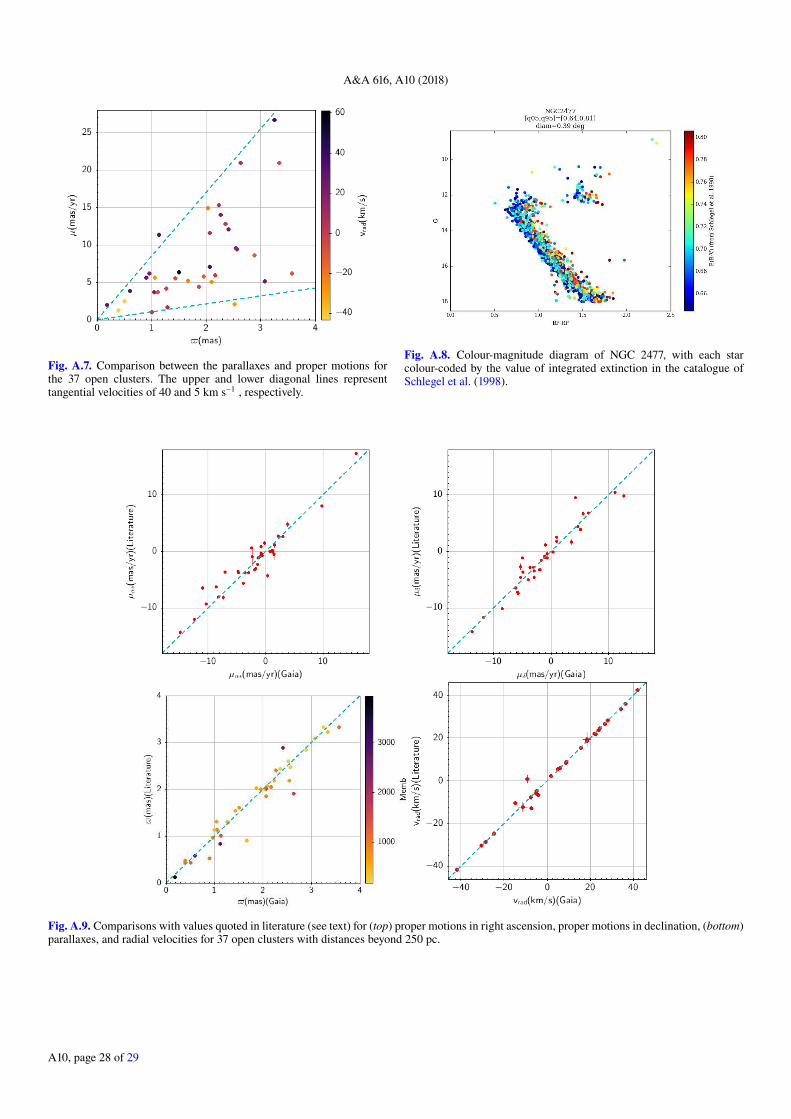
A&A 616, A10 (2018)

Fig. A.7. Comparison between the parallaxes and proper motions forthe 37 open clusters. The upper and lower diagonal lines representtangential velocities of 40 and 5 km s−1 , respectively.

Fig. A.9. Comparisons with values quoted in literature (see text) for (top) proper motions in right ascension, proper motions in declination, (bottom)parallaxes, and radial velocities for 37 open clusters with distances beyond 250 pc.

Fig. A.8. Colour-magnitude diagram of NGC 2477, with each starcolour-coded by the value of integrated extinction in the catalogue ofSchlegel et al. (1998).

A10, page 28 of 29

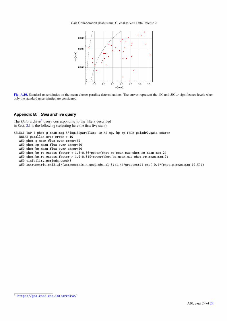
Gaia Collaboration (Babusiaux, C. et al.): Gaia Data Release 2

Fig. A.10. Standard uncertainties on the mean cluster parallax determinations. The curves represent the 100 and 500 σ significance levels whenonly the standard uncertainties are considered.

Appendix B: Gaia archive query

The Gaia archive6 query corresponding to the filters describedin Sect. 2.1 is the following (selecting here the first five stars):

SELECT TOP 5 phot_g_mean_mag+5*log10(parallax)-10 AS mg, bp_rp FROM gaiadr2.gaia_source

WHERE parallax_over_error > 10

AND phot_g_mean_flux_over_error>50

AND phot_rp_mean_flux_over_error>20

AND phot_bp_mean_flux_over_error>20

AND phot_bp_rp_excess_factor < 1.3+0.06*power(phot_bp_mean_mag-phot_rp_mean_mag,2)

AND phot_bp_rp_excess_factor > 1.0+0.015*power(phot_bp_mean_mag-phot_rp_mean_mag,2)

AND visibility_periods_used>8

AND astrometric_chi2_al/(astrometric_n_good_obs_al-5)<1.44*greatest(1,exp(-0.4*(phot_g_mean_mag-19.5)))

6 https://gea.esac.esa.int/archive/

A10, page 29 of 29