Embed Size (px)
Citation preview
Laboratoire de l’Informatique du Parallélisme
École Normale Supérieure de LyonUnité Mixte de Recherche CNRS-INRIA-ENS LYON no 5668
Load-Balancing Scatter Operationsfor Grid Computing
Stéphane Genaud,Arnaud Giersch,Frédéric Vivien
March 2003
Research Report No 2003-17
École Normale Supérieure de Lyon46 Allée d’Italie, 69364 Lyon Cedex 07, France
Téléphone : +33(0)4.72.72.80.37Télécopieur : +33(0)4.72.72.80.80
Adresse électronique :[email protected]
Load-Balancing Scatter Operations
for Grid Computing
Stéphane Genaud, Arnaud Giersch, Frédéric Vivien
March 2003
AbstractWe present solutions to statically load-balance scatter operations in par-allel codes run on grids. Our load-balancing strategy is based on themodi�cation of the data distributions used in scatter operations. Westudy the replacement of scatter operations with parameterized scatters,allowing custom distributions of data. The paper presents: 1) a generalalgorithm which �nds an optimal distribution of data across processors;2) a quicker guaranteed heuristic relying on hypotheses on communica-tions and computations; 3) a policy on the ordering of the processors.Experimental results with an MPI scienti�c code illustrate the bene�tsobtained from our load-balancing.
Keywords: parallel programming, grid computing, heterogeneous computing, load-balancing,scatter operation.
RésuméNous présentons des solutions pour équilibrer statiquement la charge desopérations � scatter � dans les codes parallèles exécutés sur les grilles.Notre stratégie d'équilibrage de charge est basée sur la modi�cation desdistributions des données utilisées dans les opérations scatter. Nous étu-dions la substitution des opérations scatter par des scatters paramétrés,permettant des distributions de données adaptées. L'article présente : 1)un algorithme général qui trouve une distribution optimale des donnéesentre les processeurs; 2) une heuristique garantie plus rapide s'appuyantsur des hypothèses sur les communications et les calculs; 3) une politiqued'ordonnancement des processeurs. Des résultats expérimentaux avec uncode scienti�que MPI illustre les gains obtenus par notre équilibrage decharge.
Mots-clés: programmation parallèle, grille de calcul, calcul hétérogène, équilibrage de charge,opération scatter.
Load-Balancing Scatter Operations for Grid Computing 1
1 Introduction
Traditionally, users have developed scienti�c applications with a parallel computer in mind, assum-ing an homogeneous set of processors linked with an homogeneous and fast network. However,grids [11] of computational resources usually include heterogeneous processors, and heterogeneousnetwork links that are orders of magnitude slower than in a parallel computer. Therefore, the ex-ecution on grids of applications designed for parallel computers usually leads to poor performanceas the distribution of workload does not take the heterogeneity into account. Hence the need fortools able to analyze and transform existing parallel applications to improve their performances onheterogeneous environments by load-balancing their execution. Furthermore, we are not willing tofully rewrite the original applications but we are rather seeking transformations which modify theoriginal source code as little as possible.
Among the usual operations found in parallel codes is the scatter operation, which is one of thecollective operations usually shipped with message passing libraries. For instance, the mostly usedmessage passing library MPI [21] provides a MPI_Scatter primitive that allows the programmer todistribute even parts of data to the processors in the MPI communicator.
The less intrusive modi�cation enabling a performance gain in an heterogeneous environmentconsists in using a communication library adapted to heterogeneity. Thus, much work has beendevoted to that purpose: for MPI, numerous projects including MagPIe [19], MPI-StarT [17], andMPICH-G2 [9], aim at improving communications performance in presence of heterogeneous net-works. Most of the gain is obtained by reworking the design of collective communication primitives.For instance, MPICH-G2 performs often better than MPICH to disseminate information held by aprocessor to several others. While MPICH always use a binomial tree to propagate data, MPICH-G2is able to switch to a �at tree broadcast when network latency is high [18]. Making the communi-cation library aware of the precise network topology is not easy: MPICH-G2 queries the underlyingGlobus [10] environment to retrieve information about the network topology that the user mayhave speci�ed through environment variables. Such network-aware libraries bring interesting re-sults as compared to standard communication libraries. However, these improvements are often notsu�cient to attain performance considered acceptable by users when the processors are also hetero-geneous. Balancing the computation tasks over processors is also needed to really take bene�t fromgrids.
The typical usage of the scatter operation is to spawn an SPMD computation section on theprocessors after they received their piece of data. Thereby, if the computation load on proces-sors depends on the data received, the scatter operation may be used as a means to load-balancecomputations, provided the items in the data set to scatter are independent. MPI provides theprimitive MPI_Scatterv that allows to distribute unequal shares of data. We claim that replacingMPI_Scatter by MPI_Scatterv calls parameterized with clever distributions may lead to great per-formance improvements at low cost. In term of source code rewriting, the transformation of suchoperations does not require a deep source code re-organization, and it can easily be automated in asoftware tool. Our problem is thus to load-balance the execution by computing a data distributiondepending on the processors speeds and network links bandwidths.
In Section 2 we present our target application, a real scienti�c application in geophysics, writtenin MPI, that we ran to ray-trace the full set of seismic events of year 1999. In Section 3 we presentour load-balancing techniques, in Section 4 the processor ordering policy we derive from a casestudy, in Section 5 our experimental results, in Section 6 the related works, and we conclude inSection 7.
2 S. Genaud, A. Giersch, F. Vivien
2 Motivating example
2.1 Seismic tomography
The geophysical code we consider is in the seismic tomography �eld. The general objective of suchapplications is to build a global seismic velocity model of the Earth interior. The various velocitiesfound at the di�erent points discretized by the model (generally a mesh) re�ect the physical rockproperties in those locations. The seismic waves velocities are computed from the seismogramsrecorded by captors located all around the globe: once analyzed, the wave type, the earthquakehypocenter, and the captor locations, as well as the wave travel time, are determined.
From these data, a tomography application reconstructs the event using an initial velocitymodel. The wave propagation from the source hypocenter to a given captor de�nes a path, thatthe application evaluates given properties of the initial velocity model. The time for the wave topropagate along this evaluated path is then compared to the actual travel time and, in a �nal step,a new velocity model that minimizes those di�erences is computed. This process is more accurate ifthe new model better �ts numerous such paths in many locations inside the Earth, and is thereforevery computationally demanding.
2.2 The example application
We now outline how the application under study exploits the potential parallelism of the compu-tations, and how the tasks are distributed across processors. Recall that the input data is a setof seismic waves characteristics each described by a pair of 3D coordinates (the coordinates of theearthquake source and those of the receiving captor) plus the wave type. With these characteristics,a seismic wave can be modeled by a set of ray paths that represents the wavefront propagation.Seismic wave characteristics are su�cient to perform the ray-tracing of the whole associated raypath. Therefore, all ray paths can be traced independently. The existing parallelization of theapplication (presented in [14]) assumes an homogeneous set of processors (the implicit target beinga parallel computer). There is one MPI process per processor. The following pseudo-code outlinesthe main communication and computation phases:
if (rank = ROOT)raydata ← read n lines from data file;
MPI_Scatter(raydata, n/P,...,rbuff,...,ROOT,MPI_COMM_WORLD);compute_work(rbuff);
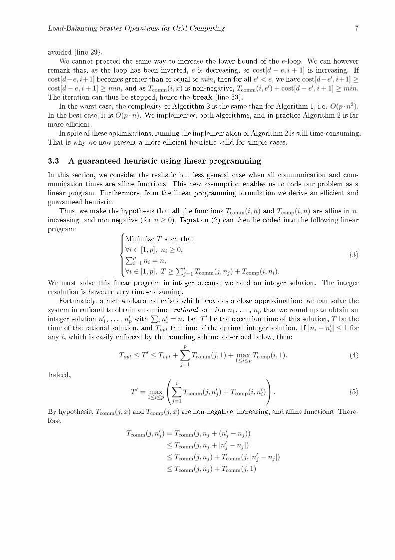
where P is the number of processors involved, and n the number of data items. The MPI_Scatterinstruction is executed by the root and the computation processors. The processor identi�ed as ROOTperforms a send of contiguous blocks of bn/P c elements from the raydata bu�er to all processors ofthe group while all processors make a receive operation of their respective data in the rbuff bu�er.For sake of simplicity the remaining (n mod P ) items distribution is not shown here. Figure 1 showsa potential execution of this communication operation, with P4 as root processor.
2.3 Hardware model
Figure 1 outlines the behavior of the scatter operation as it was observed during the applicationsruns on our test grid (described in Section 5.1). This behavior is an indication on the networkingcapabilities of the root node: it can send to at most one destination node at a time. This is thesingle-port model of [4] which is realistic for grids as many nodes are simple PCs with full-duplex
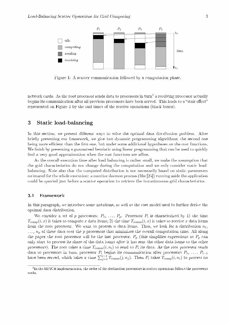
Load-Balancing Scatter Operations for Grid Computing 3
time
idle
receiving
sending
computing
t0
t1
P1 P2 P3 P4
Figure 1: A scatter communication followed by a computation phase.
network cards. As the root processor sends data to processors in turn1 a receiving processor actuallybegins its communication after all previous processors have been served. This leads to a �stair e�ect�represented on Figure 1 by the end times of the receive operations (black boxes).
3 Static load-balancing
In this section, we present di�erent ways to solve the optimal data distribution problem. Afterbrie�y presenting our framework, we give two dynamic programming algorithms, the second onebeing more e�cient than the �rst one, but under some additional hypotheses on the cost functions.We �nish by presenting a guaranteed heuristic using linear programming that can be used to quickly�nd a very good approximation when the cost functions are a�ne.
As the overall execution time after load-balancing is rather small, we make the assumption thatthe grid characteristics do not change during the computation and we only consider static load-balancing. Note also that the computed distribution is not necessarily based on static parametersestimated for the whole execution: a monitor daemon process (like [25]) running aside the applicationcould be queried just before a scatter operation to retrieve the instantaneous grid characteristics.
3.1 Framework
In this paragraph, we introduce some notations, as well as the cost model used to further derive theoptimal data distribution.
We consider a set of p processors: P1, . . . , Pp. Processor Pi is characterized by 1) the timeTcomp(i, x) it takes to compute x data items; 2) the time Tcomm(i, x) it takes to receive x data itemsfrom the root processor. We want to process n data items. Thus, we look for a distribution n1,. . . , np of these data over the p processors that minimizes the overall computation time. All alongthe paper the root processor will be the last processor, Pp (this simpli�es expressions as Pp canonly start to process its share of the data items after it has sent the other data items to the otherprocessors). The root takes a time Tcomm(i, ni) to send to Pi its data. As the root processor sendsdata to processors in turn, processor Pi begins its communication after processors P1, . . . , Pi−1
have been served, which takes a time∑i−1
j=1 Tcomm(j, nj). Then Pi takes Tcomp(i, ni) to process its
1In the MPICH implementation, the order of the destination processors in scatter operations follows the processors
ranks.
4 S. Genaud, A. Giersch, F. Vivien
share of the data. Thus, Pi ends its processing at time:
Ti =i∑
j=1
Tcomm(j, nj) + Tcomp(i, ni). (1)
The time, T , taken by our system to compute the set of n data items is therefore:
T = max1≤i≤p
Ti = max1≤i≤p
i∑j=1
Tcomm(j, nj) + Tcomp(i, ni)
, (2)
and we are looking for the distribution n1, . . . , np minimizing this duration.
3.2 An exact solution by dynamic programming
In this section we present two dynamic programming algorithms to compute the optimal datadistribution. The �rst one only assumes that the cost functions are non-negative. The second onepresents some optimizations that makes it perform far better, but under the further hypothesis thatthe cost functions are increasing.
Basic algorithm
We now study Equation (2). The overall execution time is the maximum of the execution time ofP1, and of the other processors:
T = max
(Tcomm(1, n1) + Tcomp(1, n1),
max2≤i≤p
i∑j=1
Tcomm(j, nj) + Tcomp(i, ni)
.
Then, one can remark that all the terms in this equation contain the time needed for the rootprocessor to send P1 its data. Therefore, Equation (2) can be written:
T = Tcomm(1, n1)
+ max
Tcomp(1, n1), max2≤i≤p
i∑j=2
Tcomm(j, nj) + Tcomp(i, ni)
.
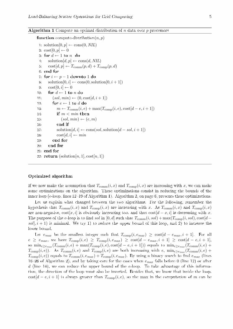
So, we notice that the time to process n data on processors 1 to p is equal to the time taken by theroot to send n1 data to P1 plus the maximum of 1) the time taken by P1 to process its n1 data;2) the time for processors 2 to p to process n − n1 data. This leads to the dynamic programmingAlgorithm 1 presented on page 5 (the distribution is expressed as a list, hence the use of the listconstructor cons). In Algorithm 1, cost[d, i] denotes the cost of the processing of d data items overthe processors Pi through Pp. solution[d, i] is a list describing a distribution of d data items overthe processors Pi through Pp which achieves the minimal execution time cost[d, i].
Algorithm 1 has a complexity of O(p · n2), which may be prohibitive. But Algorithm 1 onlyassumes that the functions Tcomm(i, x) and Tcomp(i, x) are non-negative and null whenever x = 0.
Load-Balancing Scatter Operations for Grid Computing 5
Algorithm 1 Compute an optimal distribution of n data over p processorsfunction compute-distribution(n, p)
1: solution[0, p]← cons(0,NIL)2: cost[0, p]← 03: for d← 1 to n do4: solution[d, p]← cons(d,NIL)5: cost[d, p]← Tcomm(p, d) + Tcomp(p, d)6: end for7: for i← p− 1 downto 1 do8: solution[0, i]← cons(0, solution[0, i + 1])9: cost[0, i]← 0
10: for d← 1 to n do11: (sol ,min)← (0, cost[d, i + 1])12: for e← 1 to d do13: m← Tcomm(i, e) + max(Tcomp(i, e), cost[d− e, i + 1])14: if m < min then15: (sol ,min)← (e,m)16: end if17: solution[d, i]← cons(sol , solution[d− sol , i + 1])18: cost[d, i]← min19: end for20: end for21: end for22: return (solution[n, 1], cost[n, 1])
Optimized algorithm
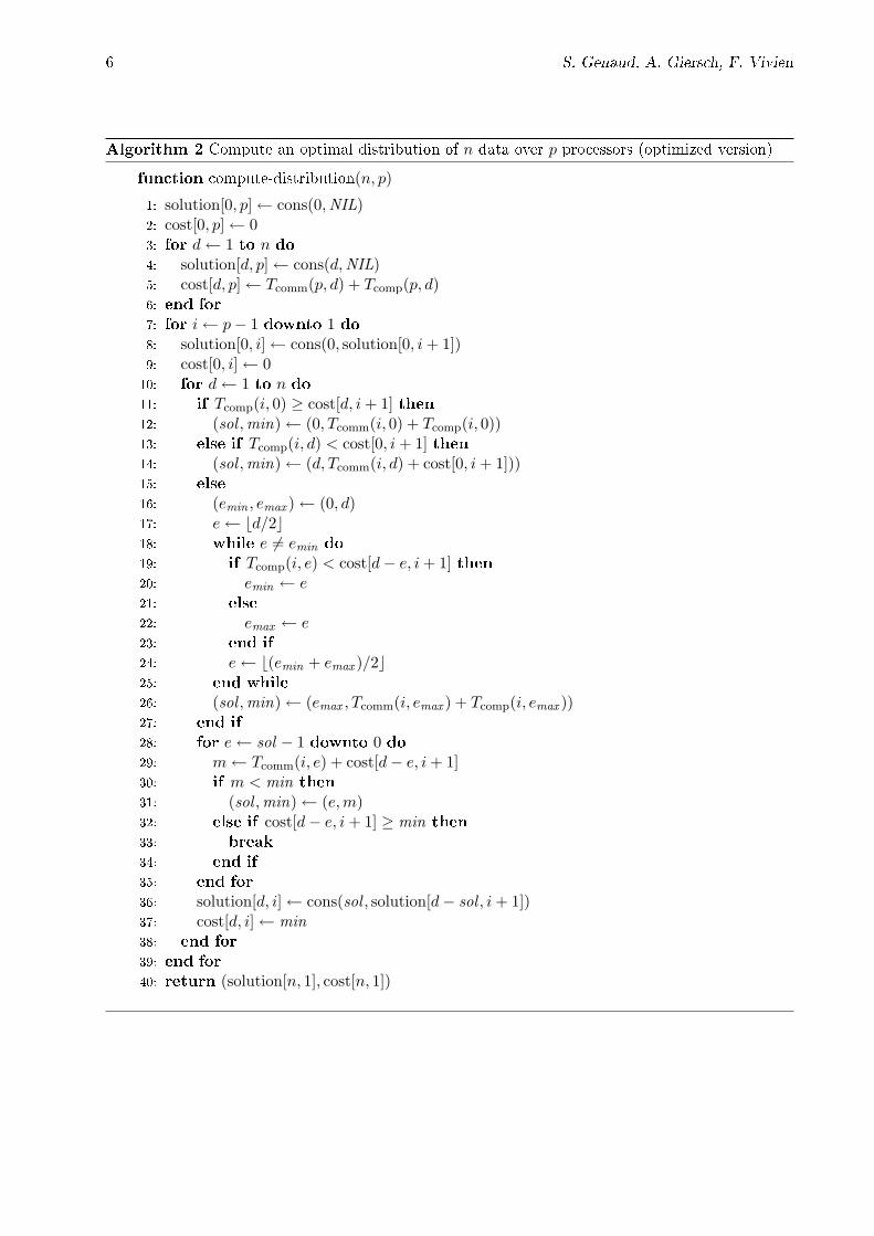
If we now make the assumption that Tcomm(i, x) and Tcomp(i, x) are increasing with x, we can makesome optimizations on the algorithm. These optimizations consist in reducing the bounds of theinner loop (e-loop, lines 12�19 of Algorithm 1). Algorithm 2, on page 6, presents these optimizations.
Let us explain what changed between the two algorithms. For the following, remember thehypothesis that Tcomm(i, x) and Tcomp(i, x) are increasing with x. As Tcomm(i, x) and Tcomp(i, x)are non-negative, cost[x, i] is obviously increasing too, and thus cost[d − x, i] is decreasing with x.The purpose of the e-loop is to �nd sol in [0, d] such that Tcomm(i, sol)+max(Tcomp(i, sol), cost[d−sol ], i + 1) is minimal. We try 1) to reduce the upper bound of this loop, and 2) to increase thelower bound.
Let emax be the smallest integer such that Tcomp(i, emax ) ≥ cost[d − emax , i + 1]. For alle ≥ emax , we have Tcomp(i, e) ≥ Tcomp(i, emax ) ≥ cost[d − emax , i + 1] ≥ cost[d − e, i + 1],so mine≥emax (Tcomm(i, e) + max(Tcomp(i, e), cost[d − e, i + 1])) equals to mine≥emax (Tcomm(i, e) +Tcomp(i, e)). As Tcomm(i, e) and Tcomp(i, e) are both increasing with e, mine≥emax (Tcomm(i, e) +Tcomp(i, e)) equals to Tcomm(i, emax ) + Tcomp(i, emax ). By using a binary search to �nd emax (lines16�26 of Algorithm 2), and by taking care for the cases when emax falls before 0 (line 12) or afterd (line 14), we can reduce the upper bound of the e-loop. To take advantage of this informa-tion, the direction of the loop must also be inverted. Besides that, we know that inside the loop,cost[d − e, i + 1] is always greater than Tcomp(i, e), so the max in the computation of m can be
6 S. Genaud, A. Giersch, F. Vivien
Algorithm 2 Compute an optimal distribution of n data over p processors (optimized version)
function compute-distribution(n, p)
1: solution[0, p]← cons(0,NIL)2: cost[0, p]← 03: for d← 1 to n do4: solution[d, p]← cons(d,NIL)5: cost[d, p]← Tcomm(p, d) + Tcomp(p, d)6: end for7: for i← p− 1 downto 1 do8: solution[0, i]← cons(0, solution[0, i + 1])9: cost[0, i]← 0
10: for d← 1 to n do11: if Tcomp(i, 0) ≥ cost[d, i + 1] then12: (sol ,min)← (0, Tcomm(i, 0) + Tcomp(i, 0))13: else if Tcomp(i, d) < cost[0, i + 1] then14: (sol ,min)← (d, Tcomm(i, d) + cost[0, i + 1]))15: else16: (emin , emax )← (0, d)17: e← bd/2c18: while e 6= emin do19: if Tcomp(i, e) < cost[d− e, i + 1] then20: emin ← e21: else22: emax ← e23: end if24: e← b(emin + emax )/2c25: end while26: (sol ,min)← (emax , Tcomm(i, emax ) + Tcomp(i, emax ))27: end if28: for e← sol − 1 downto 0 do29: m← Tcomm(i, e) + cost[d− e, i + 1]30: if m < min then31: (sol ,min)← (e,m)32: else if cost[d− e, i + 1] ≥ min then33: break34: end if35: end for36: solution[d, i]← cons(sol , solution[d− sol , i + 1])37: cost[d, i]← min38: end for39: end for40: return (solution[n, 1], cost[n, 1])
Load-Balancing Scatter Operations for Grid Computing 7
avoided (line 29).We cannot proceed the same way to increase the lower bound of the e-loop. We can however
remark that, as the loop has been inverted, e is decreasing, so cost[d − e, i + 1] is increasing. Ifcost[d−e, i+1] becomes greater than or equal to min, then for all e′ < e, we have cost[d−e′, i+1] ≥cost[d− e, i + 1] ≥ min, and as Tcomm(i, x) is non-negative, Tcomm(i, e′) + cost[d− e′, i + 1] ≥ min.The iteration can thus be stopped, hence the break (line 33).
In the worst case, the complexity of Algorithm 2 is the same than for Algorithm 1, i.e. O(p ·n2).In the best case, it is O(p ·n). We implemented both algorithms, and in practice Algorithm 2 is farmore e�cient.
In spite of these optimizations, running the implementation of Algorithm 2 is still time-consuming.That is why we now present a more e�cient heuristic valid for simple cases.
3.3 A guaranteed heuristic using linear programming
In this section, we consider the realistic but less general case when all communication and com-munication times are a�ne functions. This new assumption enables us to code our problem as alinear program. Furthermore, from the linear programming formulation we derive an e�cient andguaranteed heuristic.
Thus, we make the hypothesis that all the functions Tcomm(i, n) and Tcomp(i, n) are a�ne in n,increasing, and non-negative (for n ≥ 0). Equation (2) can then be coded into the following linearprogram:
Minimize T such that∀i ∈ [1, p], ni ≥ 0,∑p
i=1 ni = n,
∀i ∈ [1, p], T ≥∑i
j=1 Tcomm(j, nj) + Tcomp(i, ni).
(3)
We must solve this linear program in integer because we need an integer solution. The integerresolution is however very time-consuming.
Fortunately, a nice workaround exists which provides a close approximation: we can solve thesystem in rational to obtain an optimal rational solution n1, . . . , np that we round up to obtain aninteger solution n′1, . . . , n′p with
∑i n
′i = n. Let T ′ be the execution time of this solution, T be the
time of the rational solution, and Topt the time of the optimal integer solution. If |ni − n′i| ≤ 1 forany i, which is easily enforced by the rounding scheme described below, then:
Topt ≤ T ′ ≤ Topt +p∑
j=1
Tcomm(j, 1) + max1≤i≤p
Tcomp(i, 1). (4)
Indeed,
T ′ = max1≤i≤p
i∑j=1
Tcomm(j, n′j) + Tcomp(i, n′i)
. (5)
By hypothesis, Tcomm(j, x) and Tcomp(j, x) are non-negative, increasing, and a�ne functions. There-fore,
Tcomm(j, n′j) = Tcomm(j, nj + (n′j − nj))
≤ Tcomm(j, nj + |n′j − nj |)≤ Tcomm(j, nj) + Tcomm(j, |n′j − nj |)≤ Tcomm(j, nj) + Tcomm(j, 1)
8 S. Genaud, A. Giersch, F. Vivien
and we have an equivalent upper bound for Tcomp(j, n′j). Using these upper bounds to over-approximate the expression of T ′ given by Equation (5) we obtain:
T ′ ≤ max1≤i≤p
i∑j=1
(Tcomm(j, nj) + Tcomm(j, 1)) + Tcomp(i, ni) + Tcomp(i, 1)
(6)
which implies Equation (4) knowing that Topt ≤ T ′, T ≤ Topt , and �nally that:
T = max1≤i≤p
(i∑
j=1
Tcomm(j, nj) + Tcomp(i, ni)).
Rounding scheme
Our rounding scheme is trivial: �rst we round, to the nearest integer, the non integer ni which isnearest to an integer. Doing so we obtain n′i and we make an approximation error of e = n′i − ni
(with |e| < 1). If e is negative (resp. positive), ni was underestimated (resp. overestimated) by theapproximation. Then we round to its ceiling (resp. �oor), one of the remaining njs which is thenearest to its ceiling dnje (resp. �oor bnjc), we obtain a new approximation error of e = e+n′j−nj
(with |e| < 1), and so on until there only remains to approximate only one of the nis, say nk. Thenwe let n′k = nk + e. The distribution n′1, . . . , n′p is thus integer,
∑1≤i≤p n′i = d, and each n′i di�ers
from ni by less than one.
3.4 Choice of the root processor
We make the assumption that, originally, the n data items that must be processed are stored ona single computer, denoted C. A processor of C may or may not be used as the root processor.If the root processor is not on C, then the whole execution time is equal to the time needed totransfer the data from C to the root processor, plus the execution time as computed by one of theprevious algorithms and heuristic. The best root processor is then the processor minimizing thiswhole execution time, when picked as root. This is just the result of a minimization over the pcandidates.
4 A case study: solving in rational with linear communication and
computation times
In this section we study a simple and theoretical case. This case study will enable us to de�ne apolicy on the order in which the processors must receive their data.
We make the hypothesis that all the functions Tcomm(i, n) and Tcomp(i, n) are linear in n. Inother words, we assume that there are constants λi and µi such that Tcomm(i, n) = λi · n andTcomp(i, n) = µi · n. Also, we only look for a rational solution and not an integer one as we should.
We show in Section 4.3 that, in this simple case, the processor ordering leading to the shortestexecution time is quite simple. Before that we prove in Section 4.2 that there always is an optimal(rational) solution in which all the working processors have the same ending time. We also showthe condition for a processor to receive a share of the whole work. As this condition comes from theexpression of the execution duration when all processors have to process a share of the whole workand �nishes at the same date, we begin by studying this case in Section 4.1. Finally, in Section 4.4,we derive from our case study a guaranteed heuristic for the general case.
Load-Balancing Scatter Operations for Grid Computing 9
4.1 Execution duration
Theorem 1 (Execution duration) If we are looking for a rational solution, if each processor Pi
receives a (non empty) share ni of the whole set of n data items and if all processors end theircomputation at a same date t, then the execution duration is
t =n∑p
i=11
λi+µi·∏i−1
j=1µj
λj+µj
(7)
and processor Pi receives
ni =1
λi + µi·
i−1∏j=1
µj
λj + µj
· t (8)
data to process.
Proof We want to express the execution duration, t, and the number of data processor Pi mustprocess, ni, as functions of n. Equation (2) states that processor Pi ends its processing at time:Ti =
∑ij=1 Tcomm(j, nj) + Tcomp(i, ni). So, with our current hypotheses: Ti =
∑ij=1 λj · nj + µi · ni.
Thus, n1 = tλ1+µ1
and, for i ∈ [2, p],
Ti = Ti−1 − µi−1 · ni−1 + (λi + µi) · ni.
As, by hypothesis, all processors end their processing at the same time, then Ti = Ti−1 = t,ni = µi−1
λi+µi· ni−1, and we �nd Equation (8).
To express the execution duration t as a function of n we just sum Equation (8) for all valuesof i in [1, p]:
n =p∑
i=1
ni =p∑
i=1
1λi + µi
·
i−1∏j=1
µj
λj + µj
· twhich is equivalent to Equation (7). �
In the rest of this paper we note:
D(P1, . . . , Pp) =1∑p
i=11
λi+µi·∏i−1
j=1µj
λj+µj
.
and so we have t = n ·D(P1, . . . , Pp) under the hypotheses of Theorem 1.
4.2 Simultaneous endings
In this paragraph we exhibit a condition on the costs functions Tcomm(i, n) and Tcomp(i, n) which isnecessary and su�cient to have an optimal rational solution where each processor receives a non-empty share of data, and all processors end at the same date. This tells us when Theorem 1 can beused to �nd a rational solution to our system.
Theorem 2 (Simultaneous endings) Given P processors, P1, . . . , Pi, . . . , Pp, whose communi-cation and computation duration functions Tcomm(i, n) and Tcomp(i, n) are linear in n, there existsan optimal rational solution where each processor receives a non-empty share of the whole set ofdata, and all processors end their computation at the same date, if and only if
∀i ∈ [1, p− 1], λi ≤ D(Pi+1, . . . , Pp).
10 S. Genaud, A. Giersch, F. Vivien
Proof The proof is made by induction on the number of processors. If there is only one processor,then the theorem is trivially true. We shall next prove that if the theorem is true for p processors,then it is also true for p + 1 processors.
Suppose we have p+1 processors P1, . . . , Pp+1. An optimal solution for P1, . . . , Pp+1 to computen data items is obtained by giving α · n items to P1 and (1 − α) · n items to P2, . . . , Pp+1 with αin [0, 1]. The end date for the processor P1 is then t1(α) = (λ1 + µ1) · n · α.
As the theorem is supposed to be true for p processors, we know that there exists an optimalrational solution where processors P2 to Pp+1 all work and �nish their work simultaneously, ifand only if, ∀i ∈ [2, p], λi ≤ D(Pi+1, . . . , Pp+1). In this case, by Theorem 1, the time taken byP2, . . . , Pp+1 to compute (1 − α) · n data is (1 − α) · n · D(P2, . . . , Pp+1). So, the processors P2,. . . , Pp+1 all end at the same date t2(α) = λ1 · n · α + k · n · (1− α) = k · n + (λ1 − k) · n · α withk = D(P2, . . . , Pp+1).
If λ1 ≤ k, then t1(α) is strictly increasing, and t2(α) is decreasing. Moreover, we have t1(0) <t2(0) and t1(1) > t2(1), thus the whole end date max(t1(α), t2(α)) is minimized for an unique α in]0, 1[, when t1(α) = t2(α). In this case, each processor has some data to compute and they all endat the same date.
On the contrary, if λ1 > k, then t1(α) and t2(α) are both strictly increasing, thus the whole enddate max(t1(α), t2(α)) is minimized for α = 0. In this case, processor P1 has nothing to computeand its end date is 0, while processors P2 to Pp+1 all end at a same date k · n.
Thus, there exists an optimal rational solution where each of the p + 1 processors P1, . . . ,Pp+1
receives a non-empty share of the whole set of data, and all processors end their computation atthe same date, if and only if, ∀i ∈ [1, p], λi ≤ D(Pi+1, . . . , Pp+1). �
The proof of Theorem 2 shows that any processor Pi satisfying the condition λi > D(Pi+1, . . . , Pp)is not interesting for our problem: using it will only increase the whole processing time. Therefore,we just forget those processors and Theorem 2 states that there is an optimal rational solutionwhere the remaining processors are all working and have the same end date.
4.3 Processor ordering policy
As we have stated in Section 2.3, the root processor sends data to processors in turn and a receivingprocessor actually begins its communication after all previous processors have received their sharesof data. Moreover, in the MPICH implementation of MPI, the order of the destination processorsin scatter operations follows the processor ranks de�ned by the program(mer). Therefore, settingthe processor ranks in�uence the order in which the processors start to receive and process theirshare of the whole work. Equation (7) shows that in our case the overall computation time is notsymmetric in the processors but depends on their ordering. Therefore we must carefully de�nes thisordering in order to speed-up the whole computation. It appears that in our current case, the bestordering is quite simple:
Theorem 3 (Processor ordering policy) When all functions Tcomm(i, n) and Tcomp(i, n) arelinear in n, when for any i in [1, p − 1] λi ≤ D(Pi+1, . . . , Pp), and when we are only looking for arational solution, then the smallest execution time is achieved when the processors (the root processorexcepted) are ordered in decreasing order of their bandwidth (from P1, the processor connected tothe root processor with the highest bandwidth, to Pp−1, the processor connected to the root processorwith the smallest bandwidth), the last processor being the root processor.
Load-Balancing Scatter Operations for Grid Computing 11
Proof We consider any ordering P1, . . . , Pp, of the processors, except that Pp is the root processor(as we have explained in Section 3.1). We consider any permutation π of such an ordering. In otherwords, we consider any order Pπ(1), . . . , Pπ(p) of the processors such that there exists k ∈ [1, p− 2],π(k) = k + 1, π(k + 1) = k, and ∀j ∈ [1, p] \ {k, k + 1}, π(j) = j (note that π(p) = p).
We denote by tπ (resp. t) the best (rational) execution time when the processors are orderedPπ(1), . . . , Pπ(p) (resp. P1, . . . , Pp). We must show that if Pk+1 is connected to the root processorwith an higher bandwidth than Pk, then tπ is strictly smaller than t. In other words we must showthe implication:
λk+1 < λk ⇒ tπ < t. (9)Therefore, we study the sign of tπ − t.
In this di�erence, we can replace t by its expression as stated by Equation (7) as, by hypothesis,for any i in [1, p− 1], λi ≤ D(Pi+1, . . . , Pp). For tπ, things are a bit more complicated. If, for any iin [1, p− 1], λπ(i) ≤ D(Pπ(i+1), . . . , Pπ(p)), Theorems 2 and 1 apply, and thus:
tπ =n∑p
i=11
λπ(i)+µπ(i)·∏i−1
j=1µπ(j)
λπ(j)+µπ(j)
. (10)
On the opposite, if there exists at least one value i in [1, p−1] such that λπ(i) > D(Pπ(i+1), . . . , Pπ(p)),then Theorem 2 states that the optimal execution time cannot be achieved on a solution whereeach processor receives a non-empty share of the whole set of data and all processors end theircomputation at the same date. Therefore, any solution where each processor receives a non-emptyshare of the whole set of data and all processors end their computation at the same date leads toan execution time strictly greater than tπ and:
tπ <n∑p
i=11
λπ(i)+µπ(i)·∏i−1
j=1µπ(j)
λπ(j)+µπ(j)
. (11)
Equations (10) and (11) are summarized by:
tπ ≤n∑p
i=11
λπ(i)+µπ(i)·∏i−1
j=1µπ(j)
λπ(j)+µπ(j)
(12)
and proving the following implication:
λk+1 < λk ⇒n∑p
i=11
λπ(i)+µπ(i)·∏i−1
j=1µπ(j)
λπ(j)+µπ(j)
< t (13)
will prove Equation (9). Hence, we study the sign of
σ =n∑p
i=11
λπ(i)+µπ(i)·∏i−1
j=1µπ(j)
λπ(j)+µπ(j)
− n∑pi=1
1λi+µi
·∏i−1
j=1µj
λj+µj
.
As, in the above expression, both denominators are obviously (strictly) positive, the sign of σ is thesign of:
p∑i=1
1λi + µi
·i−1∏j=1
µj
λj + µj−
p∑i=1
1λπ(i) + µπ(i)
·i−1∏j=1
µπ(j)
λπ(j) + µπ(j). (14)
We want to simplify the second sum in Equation (14). Thus we remark that for any value ofi ∈ [1, k] ∪ [k + 2, p] we have:
i−1∏j=1
µπ(j)
λπ(j) + µπ(j)=
i−1∏j=1
µj
λj + µj. (15)
12 S. Genaud, A. Giersch, F. Vivien
In order to take advantage of the simpli�cation proposed by Equation (15), we decompose thesecond sum in Equation (14) in four terms: the sum from 1 to k− 1, the terms for k and k + 1, andthen the sum from k + 2 to p:
p∑i=1
1λπ(i) + µπ(i)
·i−1∏j=1
µπ(j)
λπ(j) + µπ(j)=
k−1∑i=1
1λi + µi
·i−1∏j=1
µj
λj + µj+
1λk+1 + µk+1
·k−1∏j=1
µj
λj + µj
+1
λk + µk· µk+1
λk+1 + µk+1·
k−1∏j=1
µj
λj + µj+
p∑i=k+2
1λi + µi
·i−1∏j=1
µj
λj + µj. (16)
Then we report the result of Equation (16) in Equation (14), we suppress the terms common toboth sides of the � − � sign, and we divide the resulting equation by the (strictly) positive term∏k−1
j=1µj
λj+µj. This way, we obtain that σ has the same sign than:
1λk + µk
+1
λk+1 + µk+1· µk
λk + µk− 1
λk+1 + µk+1− 1
λk + µk· µk+1
λk+1 + µk+1
which is equivalent to:λk+1 − λk
(λk + µk) · (λk+1 + µk+1).
Therefore, if λk+1 < λk, then σ < 0, Equation (13) holds, and thus Equation (9) also holds.Therefore, the inversion of processors Pk and Pk+1 is pro�table if the bandwidth from the root
processor to processor Pk+1 is higher than the bandwidth from the root processor to processor Pk.�
4.4 Consequences for the general case
So, in the general case, how are we going to order our processors? An exact study is feasible evenin the general case, if we know the computation and communication characteristics of each of theprocessors. We can indeed consider all the possible orderings of our p processors, use Algorithm 1to compute the theoretical execution times, and chose the best result. This is theoretically possible.In practice, for large values of p such an approach is unrealistic. Furthermore, in the general casean analytical study is of course impossible (we cannot analytically handle any function Tcomm(i, n)or Tcomp(i, n)).
So, we build from the previous result and we order the processors in decreasing order of thebandwidth they are connected to the root processor with, except for the root processor which isordered last. Even without the previous study, such a policy should not be surprising. Indeed, thetime spent to send its share of the data items to processor Pi is payed by all the processors from Pi
to Pp. So the �rst processor should be the one it is the less expensive to send the data to, and so on.Of course, in practice, things are a bit more complicated as we are working in integers. However,the main idea is roughly the same as we now show.
We only suppose that all the computation and communication functions are linear. Then wedenote by:
• T ratopt : the best execution time that can be achieved for a rational distribution of the n data
items, whatever the ordering for the processors.
Load-Balancing Scatter Operations for Grid Computing 13
• T intopt : the best execution time that can be achieved for an integer distribution of the n data
items, whatever the ordering for the processors.Note that T rat
opt and T intopt may be achieved on two di�erent orderings of the processors. We take
a rational distribution achieving the execution time T ratopt . We round it up to obtain an integer
solution, following the rounding scheme described in Section 3.3. This way we obtain an integerdistribution of execution time T ′ with T ′ satisfying the equation:
T ′ ≤ T ratopt +
p∑j=1
Tcomm(j, 1) + max1≤i≤p
Tcomp(i, 1)
(the proof being the same than for Equation (4)). However, T ′ being an integer solution its executiontime is obviously at least equal to T int
opt . Also, an integer solution being a rational solution, T intopt is
at least equal to T ratopt . Hence the bounds:
T intopt ≤ T ′ ≤ T int
opt +p∑
j=1
Tcomm(j, 1) + max1≤i≤p
Tcomp(i, 1)
where T ′ is the execution time of the distribution obtained by rounding up, according to the schemeof Section 3.3, the best rational solution when the processors are ordered in decreasing order ofthe bandwidth they are connected to the root processor with, except for the root processor whichis ordered last. Therefore, when all the computation and communication functions are linear ourordering policy is even guaranteed!
5 Experimental results
5.1 Hardware environment
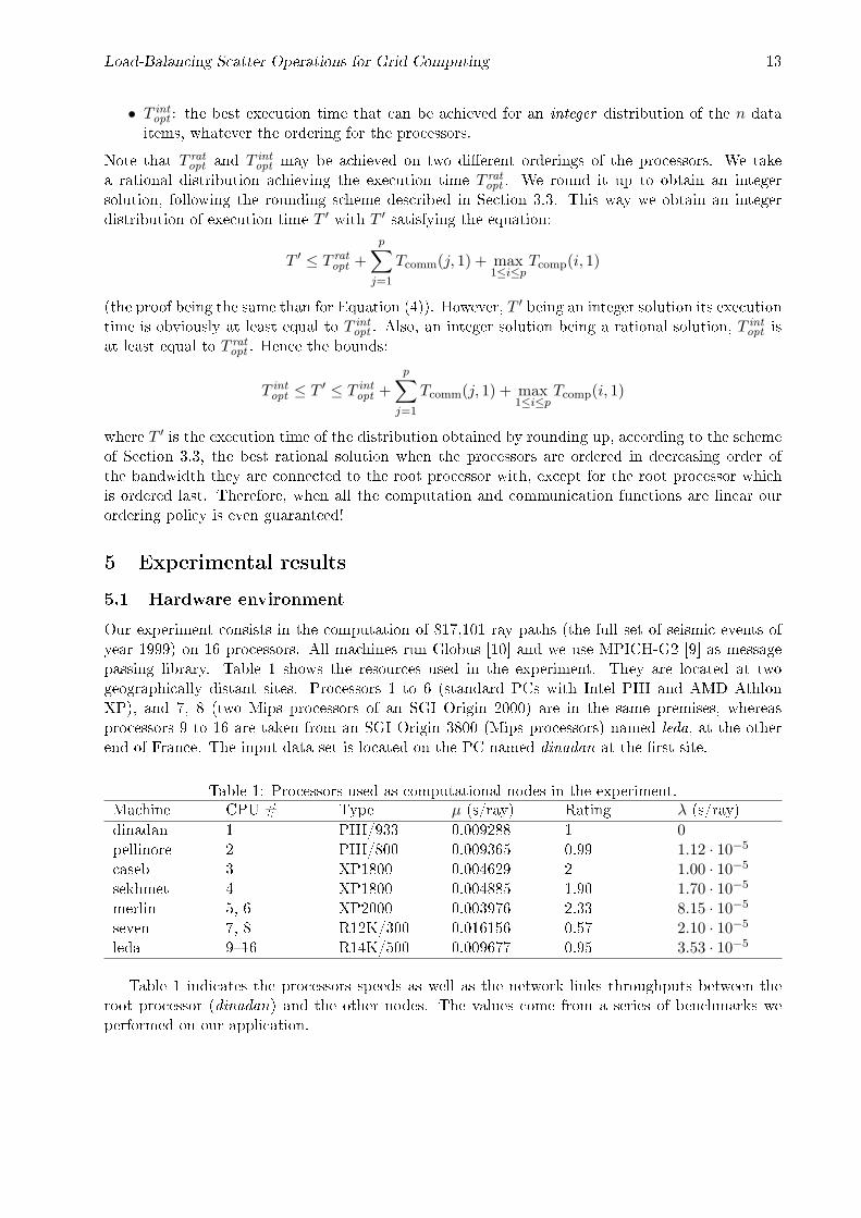
Our experiment consists in the computation of 817,101 ray paths (the full set of seismic events ofyear 1999) on 16 processors. All machines run Globus [10] and we use MPICH-G2 [9] as messagepassing library. Table 1 shows the resources used in the experiment. They are located at twogeographically distant sites. Processors 1 to 6 (standard PCs with Intel PIII and AMD AthlonXP), and 7, 8 (two Mips processors of an SGI Origin 2000) are in the same premises, whereasprocessors 9 to 16 are taken from an SGI Origin 3800 (Mips processors) named leda, at the otherend of France. The input data set is located on the PC named dinadan at the �rst site.
Table 1: Processors used as computational nodes in the experiment.Machine CPU # Type µ (s/ray) Rating λ (s/ray)dinadan 1 PIII/933 0.009288 1 0pellinore 2 PIII/800 0.009365 0.99 1.12 · 10−5
caseb 3 XP1800 0.004629 2 1.00 · 10−5
sekhmet 4 XP1800 0.004885 1.90 1.70 · 10−5
merlin 5, 6 XP2000 0.003976 2.33 8.15 · 10−5
seven 7, 8 R12K/300 0.016156 0.57 2.10 · 10−5
leda 9�16 R14K/500 0.009677 0.95 3.53 · 10−5
Table 1 indicates the processors speeds as well as the network links throughputs between theroot processor (dinadan) and the other nodes. The values come from a series of benchmarks weperformed on our application.
14 S. Genaud, A. Giersch, F. Vivien
The column µ indicates the number of seconds needed to compute one ray (the lower, the better).The associated rating is simply a more intuitive indication of the processor speed (the higher, thebetter): it is the inverse of µ normalized with respect to a rating of 1 arbitrarily chosen for thePentium III/933. When several identical processors are present on a same computer (5, 6 and 9�16)the average performance is reported.
The network links throughputs between the root processor and the other nodes are reported incolumn λ assuming a linear communication cost. It indicates the time in seconds needed to receiveone data element from the root processor. Considering linear communication costs is su�cientlyaccurate in our case since the network latency is negligible compared to the sending time of thedata blocks.
Notice that merlin, with processors 5 and 6, though geographically close to the root processor,has the smallest bandwidth because it was connected to a 10 Mbit/s hub during the experimentwhereas all others were connected to fast-ethernet switches.
5.2 Results
The experimental results of this section evaluate two aspects of the study. The �rst experimentcompares an unbalanced execution (that is the original program without any source code modi�ca-tion) to what we predict to be the best balanced execution. The second experiment evaluates theexecution performances with respect to our processor ordering policy (the processors are ordered indescending order of their bandwidths) by comparing this policy to the opposite one (the processorsare ordered in ascending order of their bandwidths).
Original application
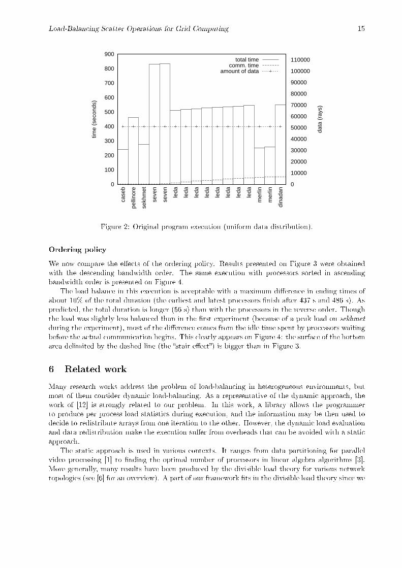
Figure 2 reports performance results obtained with the original program, in which each processorreceives an equal amount of data. We had to choose an ordering of the processors, and from theconclusion given in Section 4.4, we ordered processors by descending bandwidth.
Not surprisingly, the processors end times largely di�er, exhibiting a huge imbalance, with theearliest processor �nishing after 259 s and the latest after 853 s.
Load-balanced application
In the second experiment we evaluate our load-balancing strategy. We made the assumption thatthe computation and communication cost functions were a�ne and increasing. This assumptionallowed us to use our guaranteed heuristic. Then, we simply replaced the MPI_Scatter call bya MPI_Scatterv parameterized with the distribution computed by the heuristic. With such alarge number of rays, Algorithm 1 takes more than two days of work (we interrupted it before itscompletion) and Algorithm 2 takes 6 minutes to run on a Pentium III/933 whereas the heuristicexecution, using pipMP [8, 22], is instantaneous and has an error relative to the optimal solution ofless than 6 · 10−6!
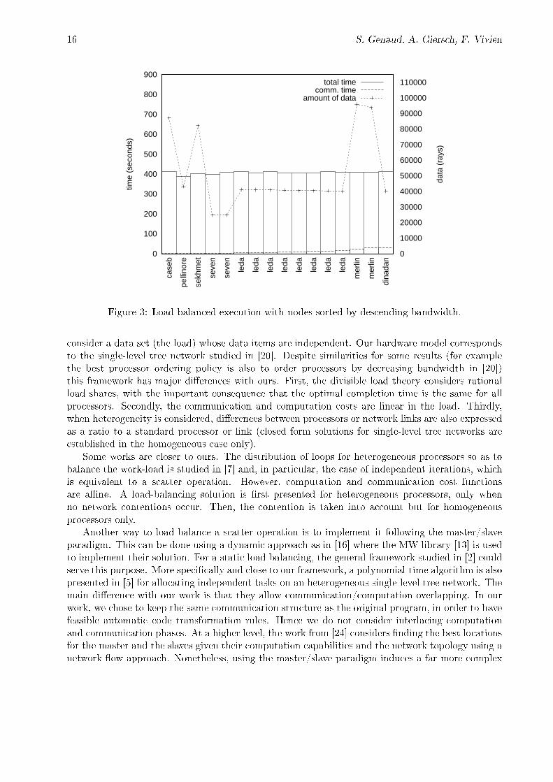
Results of this experiment are presented on Figure 3. The execution appears well balanced:the earliest and latest �nish times are 405 s and 430 s respectively, which represents a maximumdi�erence in �nish times of 6% of the total duration. By comparison to the performances of theoriginal application, the gain is signi�cant: the total execution duration is approximately half theduration of the �rst experiment.
Load-Balancing Scatter Operations for Grid Computing 15
0
100
200
300
400
500
600
700
800
900
0
10000
20000
30000
40000
50000
60000
70000
80000
90000
100000
110000
time
(sec
onds
)
data
(ra
ys)
case
b
pelli
nore
sekh
met
seve
n
seve
n
leda
leda
leda
leda
leda
leda
leda
leda
mer
lin
mer
lin
dina
dan
total timecomm. time
amount of data
Figure 2: Original program execution (uniform data distribution).
Ordering policy
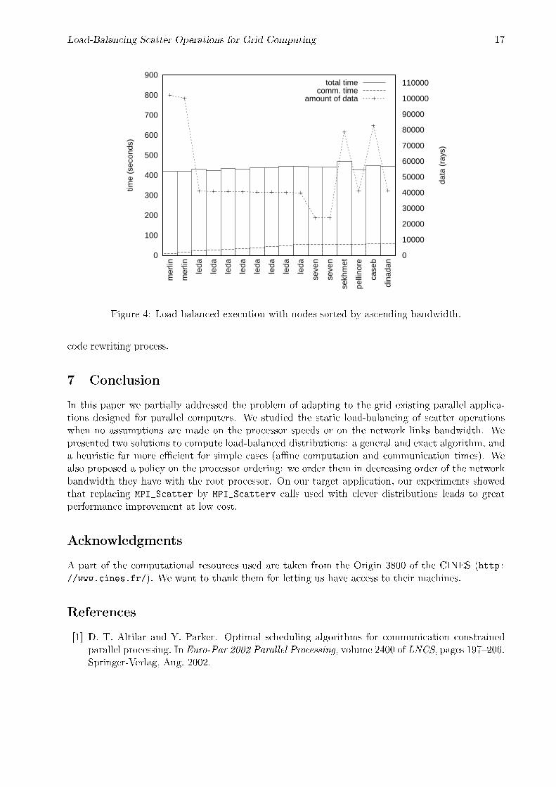
We now compare the e�ects of the ordering policy. Results presented on Figure 3 were obtainedwith the descending bandwidth order. The same execution with processors sorted in ascendingbandwidth order is presented on Figure 4.
The load balance in this execution is acceptable with a maximum di�erence in ending times ofabout 10% of the total duration (the earliest and latest processors �nish after 437 s and 486 s). Aspredicted, the total duration is longer (56 s) than with the processors in the reverse order. Thoughthe load was slightly less balanced than in the �rst experiment (because of a peak load on sekhmetduring the experiment), most of the di�erence comes from the idle time spent by processors waitingbefore the actual communication begins. This clearly appears on Figure 4: the surface of the bottomarea delimited by the dashed line (the �stair e�ect�) is bigger than in Figure 3.
6 Related work
Many research works address the problem of load-balancing in heterogeneous environments, butmost of them consider dynamic load-balancing. As a representative of the dynamic approach, thework of [12] is strongly related to our problem. In this work, a library allows the programmerto produce per process load statistics during execution, and the information may be then used todecide to redistribute arrays from one iteration to the other. However, the dynamic load evaluationand data redistribution make the execution su�er from overheads that can be avoided with a staticapproach.
The static approach is used in various contexts. It ranges from data partitioning for parallelvideo processing [1] to �nding the optimal number of processors in linear algebra algorithms [3].More generally, many results have been produced by the divisible load theory for various networktopologies (see [6] for an overview). A part of our framework �ts in the divisible load theory since we
16 S. Genaud, A. Giersch, F. Vivien
0
100
200
300
400
500
600
700
800
900
0
10000
20000
30000
40000
50000
60000
70000
80000
90000
100000
110000
time
(sec
onds
)
data
(ra
ys)
case
b
pelli
nore
sekh
met
seve
n
seve
n
leda
leda
leda
leda
leda
leda
leda
leda
mer
lin
mer
lin
dina
dan
total timecomm. time
amount of data
Figure 3: Load-balanced execution with nodes sorted by descending bandwidth.
consider a data set (the load) whose data items are independent. Our hardware model correspondsto the single-level tree network studied in [20]. Despite similarities for some results (for examplethe best processor ordering policy is also to order processors by decreasing bandwidth in [20])this framework has major di�erences with ours. First, the divisible load theory considers rationalload shares, with the important consequence that the optimal completion time is the same for allprocessors. Secondly, the communication and computation costs are linear in the load. Thirdly,when heterogeneity is considered, di�erences between processors or network links are also expressedas a ratio to a standard processor or link (closed form solutions for single-level tree networks areestablished in the homogeneous case only).
Some works are closer to ours. The distribution of loops for heterogeneous processors so as tobalance the work-load is studied in [7] and, in particular, the case of independent iterations, whichis equivalent to a scatter operation. However, computation and communication cost functionsare a�ne. A load-balancing solution is �rst presented for heterogeneous processors, only whenno network contentions occur. Then, the contention is taken into account but for homogeneousprocessors only.
Another way to load-balance a scatter operation is to implement it following the master/slaveparadigm. This can be done using a dynamic approach as in [16] where the MW library [13] is usedto implement their solution. For a static load-balancing, the general framework studied in [2] couldserve this purpose. More speci�cally and close to our framework, a polynomial-time algorithm is alsopresented in [5] for allocating independent tasks on an heterogeneous single-level tree network. Themain di�erence with our work is that they allow communication/computation overlapping. In ourwork, we chose to keep the same communication structure as the original program, in order to havefeasible automatic code transformation rules. Hence we do not consider interlacing computationand communication phases. At a higher level, the work from [24] considers �nding the best locationsfor the master and the slaves given their computation capabilities and the network topology using anetwork �ow approach. Nonetheless, using the master/slave paradigm induces a far more complex
Load-Balancing Scatter Operations for Grid Computing 17
0
100
200
300
400
500
600
700
800
900
0
10000
20000
30000
40000
50000
60000
70000
80000
90000
100000
110000
time
(sec
onds
)
data
(ra
ys)
mer
lin
mer
lin
leda
leda
leda
leda
leda
leda
leda
leda
seve
n
seve
n
sekh
met
pelli
nore
case
b
dina
dan
total timecomm. time
amount of data
Figure 4: Load-balanced execution with nodes sorted by ascending bandwidth.
code rewriting process.
7 Conclusion
In this paper we partially addressed the problem of adapting to the grid existing parallel applica-tions designed for parallel computers. We studied the static load-balancing of scatter operationswhen no assumptions are made on the processor speeds or on the network links bandwidth. Wepresented two solutions to compute load-balanced distributions: a general and exact algorithm, anda heuristic far more e�cient for simple cases (a�ne computation and communication times). Wealso proposed a policy on the processor ordering: we order them in decreasing order of the networkbandwidth they have with the root processor. On our target application, our experiments showedthat replacing MPI_Scatter by MPI_Scatterv calls used with clever distributions leads to greatperformance improvement at low cost.
Acknowledgments
A part of the computational resources used are taken from the Origin 3800 of the CINES (http://www.cines.fr/). We want to thank them for letting us have access to their machines.
References
[1] D. T. Altilar and Y. Parker. Optimal scheduling algorithms for communication constrainedparallel processing. In Euro-Par 2002 Parallel Processing, volume 2400 of LNCS, pages 197�206.Springer-Verlag, Aug. 2002.
18 S. Genaud, A. Giersch, F. Vivien
[2] C. Banino, O. Beaumont, A. Legrand, and Y. Robert. Scheduling strategies for master-slavetasking on heterogeneous processor Grids. In Applied Parallel Computing: Advanced Scienti�cComputing: 6th International Conference (PARA'02), volume 2367 of LNCS, pages 423�432.Springer-Verlag, June 2002.
[3] J. G. Barbosa, J. Tavares, and A. J. Padilha. Linear algebra algorithms in heterogeneous clusterof personal computers. In HCW 2000 [15], pages 147�159.
[4] O. Beaumont, L. Carter, J. Ferrante, A. Legrand, and Y. Robert. Bandwidth-centric allocationof independent tasks on heterogeneous platforms. In International Parallel and DistributedProcessing Symposium (IPDPS'02), page 0067. IEEE Computer Society Press, Apr. 2002.
[5] O. Beaumont, A. Legrand, and Y. Robert. A polynomial-time algorithm for allocating inde-pendent tasks on heterogeneous fork-graphs. In 17th International Symposium on Computerand Information Sciences (ISCIS XVII), pages 115�119. CRC Press, Oct. 2002.
[6] V. Bharadwaj, D. Ghose, and T. G. Robertazzi. Divisible load theory: A new paradigm forload scheduling in distributed systems. Cluster Computing, 6(1):7�17, Jan. 2003.
[7] M. Cierniak, M. J. Zaki, and W. Li. Compile-time scheduling algorithms for heterogeneous net-work of workstations. The Computer Journal, special issue on Automatic Loop Parallelization,40(6):356�372, Dec. 1997.
[8] P. Feautrier. Parametric integer programming. RAIRO Recherche Opérationnelle, 22:243�268,1988.
[9] I. Foster and N. T. Karonis. A grid-enabled MPI: Message passing in heterogeneous distributedcomputing systems. In SC 1998 [23].
[10] I. Foster and C. Kesselman. Globus: A metacomputing infrastructure toolkit. The InternationalJournal of Supercomputer Applications and High Performance Computing, 11(2):115�128, 1997.
[11] I. Foster and C. Kesselman, editors. The Grid: Blueprint for a New Computing Infrastructure.Morgan Kaufmann Publishers, Aug. 1998.
[12] W. George. Dynamic load-balancing for data-parallel MPI programs. In Message PassingInterface Developer's and User's Conference (MPIDC'99), Mar. 1999.
[13] J.-P. Goux, S. Kulkarni, J. Linderoth, and M. Yoder. An enabling framework for master-worker applications on the computational grid. In 9th IEEE International Symposium on HighPerformance Distributed Computing (HPDC'00), pages 43�50. IEEE Computer Society Press,Aug. 2000.
[14] M. Grunberg, S. Genaud, and C. Mongenet. Parallel seismic ray-tracing in a global earthmesh. In Proceedings of the International Conference on Parallel and Distributed ProcessingTechniques and Applications (PDPTA'02), volume 3, pages 1151�1157. CSREA Press, June2002.
[15] 9th Heterogeneous Computing Workshop (HCW'00). IEEE Computer Society Press, May 2000.
[16] E. Heymann, M. A. Senar, E. Luque, and M. Livny. Self-adjusting scheduling of master-workerapplications on distributed clusters. In Euro-Par 2001 Parallel Processing, volume 2150 ofLNCS, pages 742�751. Springer-Verlag, Aug. 2001.
Load-Balancing Scatter Operations for Grid Computing 19
[17] P. Husbands and J. C. Hoe. MPI-StarT: Delivering network performance to numerical appli-cations. In SC 1998 [23].
[18] N. T. Karonis, B. R. de Supinski, I. Foster, W. Gropp, E. Lusk, and J. Bresnahan. Exploitinghierarchy in parallel computer networks to optimize collective operation performance. In In-ternational Parallel and Distributed Processing Symposium (IPDPS'00), pages 377�384. IEEEComputer Society Press, May 2000.
[19] T. Kielmann, R. F. H. Hofman, H. E. Bal, A. Plaat, and R. A. F. Bhoedjang. MagPIe: MPI'scollective communication operations for clustered wide area systems. ACM SIGPLAN Notices,34(8):131�140, Aug. 1999.
[20] H. J. Kim, G.-I. Jee, and J. G. Lee. Optimal load distribution for tree network processors.IEEE Transactions on Aerospace and Electronic Systems, 32(2):607�612, Apr. 1996.
[21] MPI Forum. MPI: A message passing interface standard. Technical report, University ofTennessee, Knoxville, TN, USA, June 1995.
[22] PIP/PipLib. http://www.prism.uvsq.fr/~cedb/bastools/piplib.html.
[23] Proceedings of the 1998 ACM/IEEE conference on Supercomputing (SC'98). IEEE ComputerSociety Press, Nov. 1998.
[24] G. Shao, F. Berman, and R. Wolski. Master/slave computing on the Grid. In HCW 2000 [15],pages 3�16.
[25] R. Wolski, N. T. Spring, and J. Hayes. The network weather service: A distributed resourceperformance forecasting service for metacomputing. Future Generation Computing Systems,15(5-6):757�768, Oct. 1999.