LOAD FLOW STUDY AND TRANSIENT STABILITY STUDY OF A MULTI-MACHINE SYSTEM USING STATCOM

SURYA YERRAMILLI

B.Tech. A.I.T.A.M, Jawaharlal Nehru Technological University, India, 2006

PROJECT

Submitted in partial satisfaction of the requirements for the degree of

MASTER OF SCIENCE

in

ELECTRICAL AND ELECTRONIC ENGINEERING

at

CALIFORNIA STATE UNIVERSITY, SACRAMENTO

FALL 2009

ii

LOAD FLOW AND TRANSIENT STABILITY STUDY OF A MULTI-MACHINE SYSTEM USING STATCOM

A Project

by

SURYA YERRAMILLI Approved by: __________________________________, Committee Chair Dr. John Balachandra __________________________________, Second Reader Dr. Preetam Kumar __________________________________ Date

iii

Student: Surya Yerramilli

I certify that this student has met the requirements for format contained in the University

format manual, and that this Project is suitable for shelving in the Library and credit is to

be awarded for the Project.

_________________________, Graduate Coordinator ___________________ Dr. Preetam Kumar Date

Department of Electrical and Electronic Engineering

iv

Abstract

of

LOAD FLOW AND TRANSIENT STABILITY STUDY OF MULTI-MACHINE SYSTEM USING STATCOM

by

SURYA YERRAMILLI

In this modern age the power system is becoming increasingly large and much more

complicated in its operation. Maintaining synchronism between various parts of power

system is becoming cumbersome process, which arises stability problems in power

system operations. It’s been made mandatory to consider the stability aspects. Power

system operators should consider not only economic load dispatch but also stability

aspects which are most essential.

The load flow and the transient stability studies constitute the major analytical approach

to the study of power system and its electromechanical dynamic behavior. These studies

are carried out by numerical iterative methods, which give accurate results and can be

used for any degree of modeling sophistication.

In this project the Optimal Power flow and the classical model of the synchronous

machine are used to study the stability of the power system with and without

incorporating FACTS devices. A flexible alternating current transmission system

v

(FACTS) is a power electronic based system and other static equipment that provide

control of one or more AC transmission system parameters to enhance controllability and

increase power transfer capability [27]. With the help of FACT devices, the Power

system Performance can be improved, without any generation rescheduling or topology

changes. Moreover with the use of FACTS device in the system, the line flows can be

changed in such a way that thermal limits are not exceeded with losses minimized and

stability margins increased and even contractual requirements can be fulfilled without

violating economic dispatch. The impact of STATCOM on Optimal power flow and

transient stability will be studied in this project.

For transient stability studies the classical model is considered in this project. It is the

simplest modeling used in the power system dynamics and requires minimum amount of

data and these studies can be conducted in a relatively short interval of time at minimum

cost. Further these classical studies can be provided for useful online information.

, Committee Chair Dr.John Balachandra ____________________________ Date

vi

ACKNOWLEDGMENTS I take this opportunity to thank all the people who are responsible for the successful

completion of this project.

I express my sincere gratitude to Dr. John Balachandra, for his unending support and

encouragement and for giving me an opportunity to work under his guidance. This

project helped me learn something very new, which I haven’t learned in my coursework.

I am indebtedly thankful to Dr. Preetam Kumar, Graduate Coordinator, for offering his

helping hand as a Second- Reader and for providing his valuable suggestions to make this

project successful.

Thanks are due to all my friends on Campus who made my stay here in Sacramento

memorable: Jaipaul Vasireddy, Vijay Venkata Lakkaraju, Sriram Akurati, Vijaya Yadav,

Sridhar Nayakwadi, Navaneeth Beeram, Sankeerth Katkam, Soma NarisimhaRaju,

Gogikar Geetha Malikraj, Pranav Cherupalli, Kuladeep Jogeswar Nadiminti, Vakula

Peesari, Praveena Jakkula, Chakravarthy Kodali, Mazhar Ali, Parthiv Karri and Ashwin

Hanumakonda.

I would also like to thank Srikanth Potluri, my mentor at Intel, for his constant support

and motivation in making this project successful.

I would also like to thank all my friends at India who had supported and encouraged me

to pursue my Master’s in United States.

vii

I would like to thank my father, Kanakaji Rao; my mother, Venkata Satyavthi; and my

dear sisters Archana & Prasanna and my brother-in-law Vyakarnam Shankar for all their

faith and confidence in me to pursue a Master’s program in the United States. I am

indebted to them for their unending love and blessings throughout my work.

viii

TABLE OF CONTENTS

Page Acknowledgment…………………………………………………………………………vi

List of Figures…………………………………………………………………………….xi

List of Tables………………………………………………………………………........xiii

Chapter

1. INRODUCTION………………………………………………………………............1

1.1. Load Flow………………………………………………………………………...1

1.2. Power System Stability…………………………………………………………...2

1.3. Facts Controllers……………………………………………………...…………..3

2. FACTS IN POWER SYSTEM………...………………………………………...........4

2.1. General....................................................................................................................4

2.2. Active and Reactive power flow Principles………................................................5

2.3. Different FACTS Controllers.................................................................................9

2.4. Reactive power Compensation with STATCOM….............................................11

2.5. STATCOM Theory…...........................................................................................12

3. MODELING OF STATCOM AND POWER FLOW SOLUTION………................16

3.1. Modeling of STATCOM………………………………………………..............16

3.2. Power Flow Model……………………………………………………………...18

3.3. Matlab Simulation of Power System using Newton-Raphson Method……........20

3.3.1. Simulation without STATCOM…………………………………….........20

ix

3.3.2. Simulation with STATCOM……………………………………..............22

3.4. Power Flow solution with STATCOM………………………………………….24

4. SIMPLIFIED MATHEMATICAL MODEL OF SYNCHRONOUS MACHINE......25

4.1. General……………………………………………………………………..........25

4.2. Simplified E Model of synchronous generator……………………….................25

4.3. Representation of Loads……………………………………………………......27.

4.4. Network Performance Equations………………………………………………..28

5. MULTIMACHINE TRANSIENT STABILITY STUDY…………………………...35

5.1. Multi-Machine Transient Stability Studies...........................................................35

5.2. Classical Transient Stability Studies…………………………………………....36

5.3. Numerical Methods of solution of Swing Equation…………………………….39

5.3.1. Modified Euler’s Method………………………………………………...39

5.4. STATCOM in Power System………...…………………………………............44

5.4.1. Synchronous Generator and its Excitation System……………………....44

6. ALGORITHM AND FLOW CHART……………………………………………….47

6.1. Algorithm for Classical Transient Stability Study………………………………47

6.2. Flow Chart for Modified Euler’s Method……………………………………….49

7. RESULTS……………………………………………………………………………52

7.1. Case Study (Stable Case)………………………………………………………..52

7.2. Case Study (Unstable Case)……………………………………………………..52

8. Conclusion…………………………………………………………………………...59

x

9. Appendix A…………………………………………………………………………..61

10. Bibliography…….…………………………………………………………………...65

xi

LIST OF FIGURES

Page

1. Figure2.2.1 Model for Calculation of Real and Reactive Power flow…………….6

2. Figure2.5.1 Static Synchronous Compensator…………………………………...13

3. Figure 2.5.2 Static Synchronous Compensator V-I Characteristics …………….14

4. Figure 3.1.1VSC Connected to the AC Network VIA a SHUNT Connected Transformer………………………………………………………………………16

5. Figure 3.1.2 Shunt State Voltage Converter……………………………. ……....17

6. Figure 3.3.1 5-Bus Power System without STATCOM ………………………...21

7. Figure 3.3.2 5-Bus Power System with STATCOM…………………… ………23

8. Figure 4.1.1 Equivalent Circuit of Synchronous Machine ……………………...26

9. Figure 4.1.2 Phasor Diagram of Synchronous Machine …………………….......26

10. Figure 4.2.1 Single Line Diagram of Power system for Transient Analysis ……30

11. Figure 5.2 Representation of a Synchronous machine by constant Voltage behind Transient Reactance……………………………………………………………...38

12. Figure 5.4.1.1:Block diagram of excitation System…. …………………………45

13. Figure 6.2 Flow Chart for Modified Euler’s Method …………………………...49

14. Figure 7.1 Relative angle of Machine2 for a fault on Bus2 cleared at 0.15sec, of a 5-Bus Power system with stable case …………………………………………...53

15. Figure 7.2 Internal Voltage angle of Machines for a fault on Bus2 cleared at

0.15sec, of a 5-Bus Power system with stable case ……………………………..53 16. Figure 7.3 Relative angle of Machine2 for a fault on Bus2 cleared at 0.2sec, of a

5-Bus Power system with Unstable case ……………………………………… 54

xii

17. Figure 7.4 Internal Voltage angle of Machines for a fault on Bus2 cleared at 0.2sec, of a 5-Bus Power system with Unstable case …………………………...54

18. Figure A.1 Single Line Diagram Representation of 5 bus system for transient

Stability calculation……………………………………………………………...61

xiii

LIST OF TABLES

Page

1. Table 7.1 Simulation results for a fault on Bus2 cleared at 0.15sec, of a 5-Bus System with stable case …………………………………………………………55

2. Table 7.2 Simulation results for a fault on Bus2 cleared at 0.15sec, of a 5-Bus

System with stable case …………………………………………………………56

3. Table 7.3 Simulation results for a fault on Bus2 cleared at 0.2sec, of a 5-Bus System with Unstable case ………………………………………………………57

4. Table 7.4 Simulation results for a fault on Bus2 cleared at 0.2sec, of a 5-Bus

System with Unstable case ………………………………………………………58

5. Table A.1 Impedance and Line Charging Admittance for a 5-Bus System……...62

6. Table A.2 Scheduled Generation and Loads and Specified Bus Voltages for a 5-Bus system…….....................................................................................................63

7. Table A.3 Inertia Constants, direct axis Transient Reactance…………………...63

8. Table A.4 Static Synchronous Compensator Data…………………………….....64

1

Chapter 1

INTRODUCTION

1.1 Load Flow

In present day’s scenario of highly complex and interconnected power systems, there is a

great need to improve electric power utilization while still maintaining reliability and

security. Load flow study in power system parlance is the steady state solution of the

power system network. The main information obtained from this study comprises the

magnitudes and phase angles of load bus voltages, reactive powers at generators buses,

real and reactive power flow on transmission lines, other variables being known. Usually

a generating station is not situated near the load center, but it may be away from load

center due to various circumstances. In order to meet the ever-growing power demand,

utilities prefer to rely on already existing generation and power export/import

arrangements instead of building new transmission lines which are restricted by various

constraints. On the other hand, power flows in some of the transmission lines are well

below their thermal limits, while certain lines are overloaded, which has an overall effect

of deteriorating voltage profiles and decreasing system stability and security. In addition,

existing traditional transmission facilities, in most cases, are not designed to handle the

control requirements of complex, highly interconnected power systems. This overall

situation requires the review of traditional transmission methods and practices, and the

creation of new concepts, which would allow the use of existing generation, and

transmission lines up to their full capabilities without reduction in system stability and

2

security. Another reason that is forcing the review of traditional transmission methods is

the tendency of modern power systems to follow the changes in today’s global economy

that are leading to deregulation of electrical power markets in order to stimulate

competition between utilities.[34, 35]

1.2 Power System Stability

Modern Electric Power system is a complex network of synchronous generators,

transmission lines and loads. [21] With changes in generation schedules and load, the

system characterstics will vary. Electrical Utilities started as stand-alone systems and

with increasing growth in the neighboring utilities and upon their addition to the network

began to form high interconnected systems. This facilitated the need to draw on each

other’s generation reserves in required times. The interconnection improved reliability

but has given birth to instability issues as the disturbances can propagate through the

system. Depending on the magnitude of disturbance the system can become transiently

unstable. A good power system should have the ability to regain its normal operating

conditions even after the disturbance, as the ability to supply uninterrupted electricity

determines the quality of a power system. Stability of a power system is considered as a

very important aspect for research. [1, 2, 3, 21].

Power system stability can be defined as the ability of synchronous machines to remain in

synchronism with each other following a major disturbance [1]. The possible

3

disturbances being the line faults, generator, line outages, load switching and etc…

Stability is characterized by the capability of power system to remain in synchronism for

the possible disturbances. The stability studies are classified into steady state stability,

transient stability and slowly growing stability depending on the order of magnitude and

type of disturbance. [4, 5, 6, 21]. The transient stability of a system can be improved by

using FACT Controllers.

1.3 FACTS Controllers

Flexible AC Transmission Systems (FACTS) devices as defined by IEEE as “power

electronic based controllers and other static equipment which can regulate the power flow

and transmission voltage through rapid control action”. In earlier days power system

control was only based on generator control and the controlling ability on the

transmission lines was meager. With advent of FACTS controllability of transmission

line impedance, both series and shunt was made possible. The performance of long

distance AC transmission lines can be improved by using FACTS devices in the Power

system. The technology was later developed using FACTS devices to regulate Power

flow in the system as well. Power transmitted in a power system depends upon the

impedance in lines and on the voltages and angles at both sending and receiving ends.

Different FACTS controllers can influence these parameters to regulate the power flow in

interconnected systems. STATCOM a shunt connected FACTS application can facilitate

the fast voltage control and the reactive power control in a Power system. [27, 28, 29, 21]

4

Chapter 2

FACTS IN POWER SYSTEM

2.1 General

The controllability on one or more power flow arguments aroused the possibility to

control active as well as reactive power flow in the transmission systems. The arguments

referred in the power flow are line impedance, magnitude of voltages on both sending

and receiving end and also the angles between voltages. [23, 30]

In earlier times, power systems were designed to be self-sufficient and were very simple

interconnected systems. The AC power flow between the power systems was rarely

unusual as the AC transmission lines did not have the capability to handle dynamic

changes in the system and these problems were usually solved by adapting generous

stability margins. But now in today’s world with the advent of high complex

interconnected systems the system loadability and security can be increased to an extent

by number of different approaches. The common practice is to install the shunt capacitors

on the receiving end side to improve the voltage levels and also insertion of series

capacitors to reduce transmission line reactance, which would eventually increase the

power transfer capability of lines. To introduce an additional phase shift between sending

and receiving end voltages, phase shifting transformers are applied. The variability of

these parameters were regulated mechanically and therefore the regulation was slow. By

mechanically varying the parameters was good enough for the steady state operation but

with increase in complexity of the Power system dynamic operation was pre-dominant

5

and the time response as in varying parameters mechanically is too slow to damp the

transient oscillations. [14, 15, 18, 31]

This concept and advances in the field of power electronics led to a new approach

introduced by the Electric Power Research Institute (EPRI). Called Flexible AC

Transmission Systems or simply FACTS, it was an answer to a call for a more efficient

use of already existing resources in present power systems while maintaining and even

improving power system security. [30.31]

2.2 Basic Principles of Active and Reactive Power Flow Control

Active (real) and reactive power in a transmission line depend on the voltage magnitudes

and phase angles at the sending and receiving ends as well as line impedance. To

understand the basic concept behind the FACTS controllers as simple model is

considered in Fig 2.2.1.The sending and receiving end voltages are assumed to be fixed

and can be interpreted as points in large power systems where voltages are “stiff”.

Assuming that the resistance of high voltage transmission lines are very small, there is

equivalent reactance connected in between sending and receiving ends. The receiving

end is modeled as an infinite bus with a fixed angle of 0 . [23, 28, 34]

*IVjQPS RRRR ……………… (2.2.1)

sinX

VVP RS

R ………………. (2.2.2)

6

X

VVVQ RRS

R

2cos ……………….. (2.2.3)

Fig 2.2.1: Model for Calculation of Real and Reactive Power flow [23]

Similarly, for the sending end:

sinsin maxPX

VVP RS

S …………… (2.2.4)

X

VVVQ RSS

S

cos2

…………… (2.2.5)

7

Where VS and VR are the magnitudes (in RMS values) of sending and receiving end

voltages, respectively, where is the phase-shift between sending and receiving end

voltages. [28, 32, 34]

The system is assumed to be a lossless system and so the equations for sending and

receiving active power flows, PS and PR, are equal. The maximum active power transfer

occurs, for the given system, at a power or load angle equal to 90 which can be seen in

the figure 1.1(a). Maximum power occurs at a different angle if the transmission losses

are included. The system is stable or unstable depending on whether the derivative

dP/d is positive or negative. The steady state limit is reached when the derivative is

zero. [28, 29, 32, 34]

In practice, a transmission system is never allowed to operate close to its steady state

limit, as certain margin must be left in power transfer in order for the system to be able to

handle disturbances such as load changes, faults, and switching operations. The

intersection between a load line representing sending end mechanical (turbine) power and

the demand line defines the steady state value of . The angle can be increased by a small

increase in mechanical power at the sending end. With increasing load demands the angle

goes beyond 90 and results in less power transfer. This accelerates the generator and

further increases the angle making the system unstable. However, the increased angle

increases the electric power to correlate the mechanical increased power. The concepts of

8

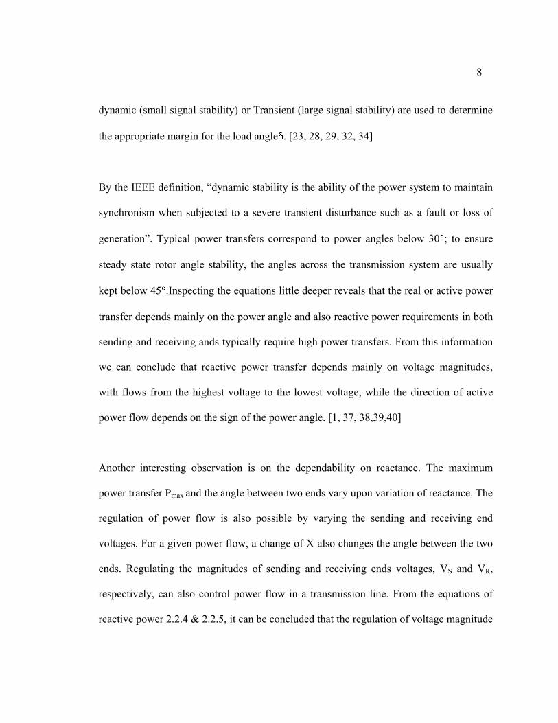
dynamic (small signal stability) or Transient (large signal stability) are used to determine

the appropriate margin for the load angle . [23, 28, 29, 32, 34]

By the IEEE definition, “dynamic stability is the ability of the power system to maintain

synchronism when subjected to a severe transient disturbance such as a fault or loss of

generation”. Typical power transfers correspond to power angles below 30 ; to ensure

steady state rotor angle stability, the angles across the transmission system are usually

kept below 45 .Inspecting the equations little deeper reveals that the real or active power

transfer depends mainly on the power angle and also reactive power requirements in both

sending and receiving ands typically require high power transfers. From this information

we can conclude that reactive power transfer depends mainly on voltage magnitudes,

with flows from the highest voltage to the lowest voltage, while the direction of active

power flow depends on the sign of the power angle. [1, 37, 38,39,40]

Another interesting observation is on the dependability on reactance. The maximum

power transfer Pmax and the angle between two ends vary upon variation of reactance. The

regulation of power flow is also possible by varying the sending and receiving end

voltages. For a given power flow, a change of X also changes the angle between the two

ends. Regulating the magnitudes of sending and receiving ends voltages, VS and VR,

respectively, can also control power flow in a transmission line. From the equations of

reactive power 2.2.4 & 2.2.5, it can be concluded that the regulation of voltage magnitude

9

has much more influence over the reactive power flow than the active power flow. [1, 37,

38, 39, 40]

2.3 Different FACTS Controllers

Basically the family of FACTS controllers is classified into two types. [27, 32, 33, 36]

(i) Series Controllers

(ii) Shunt Controllers

Definitions for various Series Controllers:

(i) Static Synchronous Series Compensator (SSSC): A static, synchronous generator

operated without an external electric energy source as a series compensator whose

output voltage is in quadrature with, and controllable independently of, the line

current for the purpose of increasing or decreasing the overall reactive voltage

drop across the line and thereby controlling the transmitted electric power. The

S3C may include transiently rated energy storage or energy absorbing devices to

enhance the dynamic behavior of the power system by additional temporary real

power compensation, to increase or decrease momentarily, the overall real

(resistive) voltage drop across the line.

(ii) Thyristor Controlled Series Capacitor (TCSC): A capacitive reactance

compensator which consists of a series capacitor bank shunted by thyristor

controlled reactor in order to provide a smoothly variable series capacitive

reactance.

10

(iii) Thyristor Controlled Series Reactor (TCSR): An inductive reactance compensator

which consists of a series reactor shunted by a thyristor controlled reactor in order

to provide a smoothly reactor in order to provide a smoothly variable series

inductive reactance.

(iv) Thyristor Switched Series Capacitor (TSSC): A capacitive reactance compensator

which consists of a series capacitor bank shunted by thyristor switched reactor to

provide a step-wise control of series capacitive reactance.

(v) Thyristor Switched Series Reactor (TSSR): An inductive reactance compensator

which consists of series reactor shunted by thyristor switched reactor in order to

provide a step-wise control of series inductive reactance.

Definitions of various Shunt Controllers:

(i) Battery Energy Storage System (BESS): A chemical-based energy storage system

using shunt connected, voltage sourced converters capable of rapidly adjusting the

amount of energy which is supplied to or absorbed from an ac system.[32]

(ii) Static Synchronous Compensator (STATCOM): A static synchronous generator

operated as a shunt-connected static var compensator whose capacitive or

inductive output current can be controlled independent of the ac system voltage.

(iii) Static Synchronous Generator(SSG): A static, self-commutated switching power

converter supplied from an appropriate electric energy source and operated to

produce a set of adjustable multi-phase output voltages, which may be coupled to

11

an ac power system for the purpose of exchanging independently controllable real

and reactive power.

(iv) Static Var Generator or Absorber (SVG): A static electrical device, equipment, or

system that is capable of drawing controlled capacitive and/or inductive current

from an electrical power system and thereby generating or absorbing reactive

power.

(v) Thyristor Controlled Reactor (TCR): A shunt-connected, thyristor-controlled

inductor whose effective reactance is varied in a continuous manner by partial-

conduction control of the thyristor valve.

(vi) Thyristor Switched Capacitor (TSC): A shunt-connected, thyristor-switched

capacitor whose effective reactance is varied in a step-wise manner by full or zero

conduction operation of the thyristor valve.

(vii) Thyristor Switched Reactor (TSR): A shunt-connected, thyristor-switched

inductor whose effective reactance is varied in a step-wise manner by full or zero

conduction operation of the thyristor valve.

2.4 Reactive power compensation with STATCOM

The amount of reactive power compensation provided by any FACTS device depends on

the voltage at the bus. STATCOM can provide the maximum rated compensating current

even at very low voltages. STATCOM also are equipped with transient capability which

is available for a short period of time and this extra capability allows STATCOM to

decide the maximum reactive power that can be supplied. [41]

12

2.5 STATCOM Theory:

STATCOM defined by IEEE as “A static synchronous generator operated as a shunt

connected static var compensator whose capacitive voltage or inductive output current

can be controlled independent of the ac system voltage.” [33]

A STATCOM is a controlled reactive power source. It provides voltage support by

generating or absorbing reactive power at the point of common coupling without the need

of large external or capacitor banks. The basic voltage source converter scheme is shown

in figure 2.5.1. [23, 37]

13

Fig 2.5.1: Static Synchronous Compensator [23,37]

The charged capacitor Cdc provides a dc voltage to the converter, which produces a set of

controllable three phase out put voltages with frequency of the ac power system. By

varying the amplitude of the output voltage U, the reactive power exchange between the

converter and the AC system can be controlled. If the amplitude of the output voltage U

is increased above that of the AC system UT, a leading current is produced, i.e. the

STATCOM is seen as a conductor by the system and reactive power is generated. By

decreasing the amplitude of the output voltage below that of AC system, a lagging

14

current results and the STATCOM is seen as an inductor. In this case reactive power is

absorbed. If the amplitudes are equal no power exchange takes place. [23.37]

A practical converter is not lossless. The mechanism of phase angle adjustment can also

be used to control the reactive power generated or absorbed by increasing or decreasing

the capacitor voltage UDC and thereby the output voltage U. The derivation of the formula

for the transmitted active power employs considerable calculations. [23.37]

Fig 2.5.2: Static Synchronous Compensator V-I Charecterstics [33]

15

The characteristics of STATCOM shown in fig 2.6.1tells very clearly that it has the

ability to support a very low system voltage; down to about 0.15 per unit, which is the

value associated with the coupling transformer reactance. This is in strong contrast with

that of a SVC when compared, which at full capacitive output becomes an uncontrolled

capacitor bank. A STATCOM can support system voltage at extremely low voltage

conditions as long as the dc capacitor can retain enough energy to supply losses. [23, 32,

33, 37].

16

Chapter 3

MODELING OF STATCOM AND POWER FLOW SOLUTION

3.1 Modeling of STATCOM:

The STATCOM is comprised of one voltage controlled source converter along with its

associated shunt connected transformer. As there are no moving parts in STATCOM, it

can be considered as a STATIC counterpart of rotating synchronous condenser. The

absence of mechanical rotating parts makes STATCOM generate or absorb power at a

faster rate unlike a regular synchronous generators [22, 42]

Fig 3.1.1: VSC CONNECTED TO THE AC NETWORK VIA A SHUNT CONNECTED

TRANSFORMER [22]

17

Fig 3.1.2: SHUNT SOLID STATE VOLTAGE SOURCE [22]

The figures 3.1.1 and 3.1.2 represents the schematic view of STATCOM and the

equivalent circuit of it respectively. Fig 3.1.2 also corresponds The equivalent circuit

corresponds to the Thevenin equivalent as seen from bus k, with the voltage source EvR

being the fundamental frequency component of the VSC output voltage, resulting from

the product of VDC and ma. [22, 42]

In steady-state fundamental frequency studies the STATCOM may be represented in the

same way as a synchronous condenser, which in most cases is the model of a

synchronous generator with zero active power generation. A more flexible model may be

realized by representing the STATCOM as a variable voltage source ErR, for which the

magnitude and phase angle may be adjusted, using a suitable iterative algorithm, to

satisfy a specified voltage magnitude at the point of connection with the AC network.

18

The shunt voltage source of the three-phase STATCOM may be represented by:

Ep

rR= Vp

rR(cosδp

rR+jsinδp

rR).

Where p indicates phase quantities. a, b, c. The voltage magnitude, Vp

rR is given

maximum and minimum limits, which are a function of the STATCOM capacitor rating.

However δp

rR may take any value between 0 and 2п radians. With reference to the

equivalent circuit shown in fig and assuming three-phase parameters, the following

transfer admittance equation can be written:

[Ik ] = [YrR - YrR] [Vk EvR]T

Where Ik = [Ik a∟γ k

a Ik

b∟γ k

a Ik

c∟γ K

a ]T

EvR= [VarR∟θδ

arRk V

brRk∟θδ

brRk V

crRk∟θδ

crRk ]

T

and YrR is a diagonal matrix with YarR, Y

brR, and Y

crR in the principal diagonal.[22,42]

3.2 POWER FLOW MODEL:

The power flow equations for the STATCOM are derived below from first principle and

assuming the following voltage source representations.

ErR= VrR (cosδrR+jsinδrR)

Based on the shunt connection shown in figure above, the following may be written

SvR= VvR I*vR = VvR Y*vR(V*vR- V*K)

19

The simplified model of active and reactive power equations are below. For a converter

and bus K, respectively:

PvR = V2

vRGvR + VvR Vk [GvRcos (δvR – θk) + BvRsin (δvR – θk)],

QvR = -V2

vRBvR + VvR Vk [GvRsin (δvR – θk) - BvRcos (δvR – θk)],

Pk = V2

kGvR + Vk VvR [GvRcos (θk– δvR) + BvRsin (θk– δvR)],

Qk = -V2

kBvR + Vk VvR [GvRsin (θk– δvR) - BvRcos (θk– δvR)].

Using these power equations, the linearized STATCOM model is given below, where the

voltage magnitude VvR and phase angle δvR are taken to be the state variables.[22,42]

∆Pk ∂Pk ∂PkVk ∂Pk ∂Pk VvR

∂θk ∂Vk ∂δ vR ∂VvR ∆θk

∆Qk ∂Qk ∂QkVk ∂Qk ∂QkVvR ∆Vk

∂θk ∂Vk ∂δ vR ∂VvR Vk

=

∆PvR ∂PvR ∂PvRVk ∂PvR ∂PvRVvR

∂θk ∂Vk ∂δ vR ∂VvR ∆δvR

∆QvR ∂QvR ∂QvRVk ∂QvR ∂QvRVvR ∆VvR

∂θk ∂Vk ∂δ vR ∂VvR VvR

20

3.3 MATLAB SIMULATION OF 5-BUS POWER SYTEM USING NEWTON-

RAPHSON’S METHOD:

The simulations in this book for power flow are done by using the matlab code available

for load flow in Acha, C Fuerte-Esquivel, C. R., Ambriz-Perez, H. and Anglese-

Camacho, C book [22]. The simulations are carried out in matlab and compared with

IEEE test results.

3.3.1 SIMULATION WITHOUT STATCOM:

3.3.1(i) SIMULATION RESULTS FROM MATLAB:

NODAL

VOLTAGE

NORTH

SOUTH

LAKE

MAIN

ELM

MAGNITUDE

(PU)

1.06

1.00

0.9841

0.9841

0.9717

PHASE

ANGLE(DEG)

0.00

-2.0612

-4.6367

-4.9570

-5.7649

3.3.1 (ii) IEEE TEST CASE RESULTS:

NODAL

VOLTAGE

NORTH

SOUTH

LAKE

MAIN

ELM

MAGNITUDE

(PU)

1.06

1.00

0.987

0.984

0.972

PHASE

ANGLE(DEG)

0.00

-2.06

-4.56

-4.96

-5.77

21

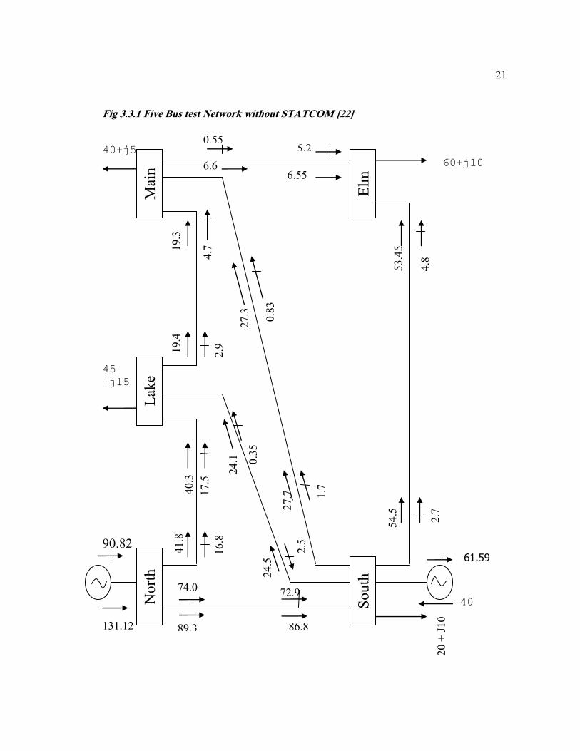
Fig 3.3.1 Five Bus test Network without STATCOM [22] 40+j5

60+j10

45

+j15

90.82 61.59

40

131.12

27.7

54.5

2.7

86.8

74.0

16.8

41.8

Nort

h

South

E

lm

Mai

n

Lak

e

89.3

20 +

J10

24.5

2.5

1.7

40.3

24.1

0.3

5

17.5

19.4

2.9

19.3

4.7

0.8

3

27.3

6.6

0.55

6.55

53.4

5

4.8

5.2

72.9

22

3.3.2 SIMULATION WITH STATCOM:

3.3.2 (i) SIMULATION RESULTS:

NODAL

VOLTAGE

NORTH

SOUTH

LAKE

MAIN

ELM

MAGNITUDE

(PU)

1.06

1.00

1.00

0.9944

0.9752

PHASE

ANGLE(DEG)

0.00

-2.0533

-4.8379

-5.1073

5.7975

3.3.2 (ii) IEEE TEST CASE RESULTS:

NODAL

VOLTAGE

NORTH

SOUTH

LAKE

MAIN

ELM

MAGNITUDE

(PU)

1.06

1.00

1.00

0.994

0.975

PHASE

ANGLE(DEG)

0.00

-2.05

-4.83

-5.11

-5.8

23

Fig 3.3.2 Five Bus test Network Upgraded with STATCOM [22]

4.3 40+j5

60+j10

45

+j15

85.4 78.1

40

131.12

27.6

54.5

2.7

74.0

86.6

74.1

11.3

41.9

2

Nort

h

South

E

lm

Mai

n

Lak

e

89.2

20 +

J10

24.5

9.5

7.3

40.5

4

24.1

6.7

12.4

19.6

4

11.2

20.5

19.6

14.0

4.7

27.2

6.8

6.78

7.9

54.3

2.1

24

3.4 POWER FLOW SOLUTION WITH STATCOM:

The results above clearly shows the modeling of STATCOM for power flow studies

provide better performance for the enhancement of dynamic and transient stability. The

Power flow results indicate that, the STATCOM generates 20.5 MVAR in order to keep

the Voltage magnitude at 1.p.u at Lake Bus. The slack generator reduces its reactive

power generation by almost 6% compared with the base case, and the reactive power

exported from North to Lake reduces by more than 30%. The largest reactive power flow

takes place in the transmission line connecting North and South. And the generator

connected at South increases its share of reactive power absorption compared with the

base case. So, in summary the power flow results shows that STATCOM generates

reactive power and maintains flat voltage profile. Active power flows are marginally

affected and reactive is generated locally with installation of STATCOM. This proves

that complex power flow can be controlled with STATCOM and the power flow can be

controlled rapidly and in a flexible way by using it. [22]

25

Chapter 4

SIMPLIFIED MATHEMATICAL MODEL OF SYNCHRONOUS MACHINE

4.1 General:

In transient stability studies, particularly those involving short periods of analysis in the

order of a second or less, a synchronous machine can be represented by a voltage source,

in back of transient reactance, that is constant in magnitude but changes its angular

position. This representation neglects the effect of saliency and assumes constant flux

linkages and a small change in speed [1, 3,26]

4.2 Simplified E' Model of Synchronous Machine:

tdtar IxjIrEE …………………. (4.2.1)

Where

E1 = Voltage back of transient reactance

Et = Machine terminal voltage

It = Machine terminal current

ra = armature resistance

x1

d = transient reactance

The representation of the synchronous machine used for network solutions and the

corresponding phasor diagram are shown in figure (4.1).

26

The saliency and changes in the field flux linkages can be taken into account by

representing the effects of the three-phase ac quantities of a synchronous machine by

components acting along the direct and quadrature axes. The direct axis is along the

center line of the machine pole and the quadrature axis leads the direct axis by 90

electrical degrees. [1,3,26]

tE

ta Ir

td Ijx1

1E

tI

Figure 4.1.2 Phasor diagram of synchronous machine[1]

1E

It

tE

Figure 4.1.1 Equivalent circuit of synchronous machine[1]

1

dx ar

27

4.3 Representations of loads:

Power system loads other than motors represented by equivalent circuits, can be treated

in several ways during the transient period .The commonly used representations are either

static impedances or admittance to ground, constant current at fixed power factor,

constant real and reactive power, or a combination of these representations. [1,3,26]

The constant power load is either equal to the scheduled real and reactive busload or is a

percentage of the specified values in the case of a combined representation. The

parameters associated with static impedance and constant current representations are

obtained from a load flow solution for the power system prior to a disturbance. The initial

value of the current for the constant current representation is obtained from [1,3,26]

p

LpLp

PoE

jQPI

Where Plp and Qlp are the scheduled busloads and Ep is the calculated bus voltage. The

current Ipo flows from bus P to ground i.e. to bus zero. The magnitude and power factor

angle of Ipo remain constant.[1,3,26]

The static admittance ypo, used to represent the load at bus P can obtained from equation

(Ep –Eo)*ypo=Ipo

28

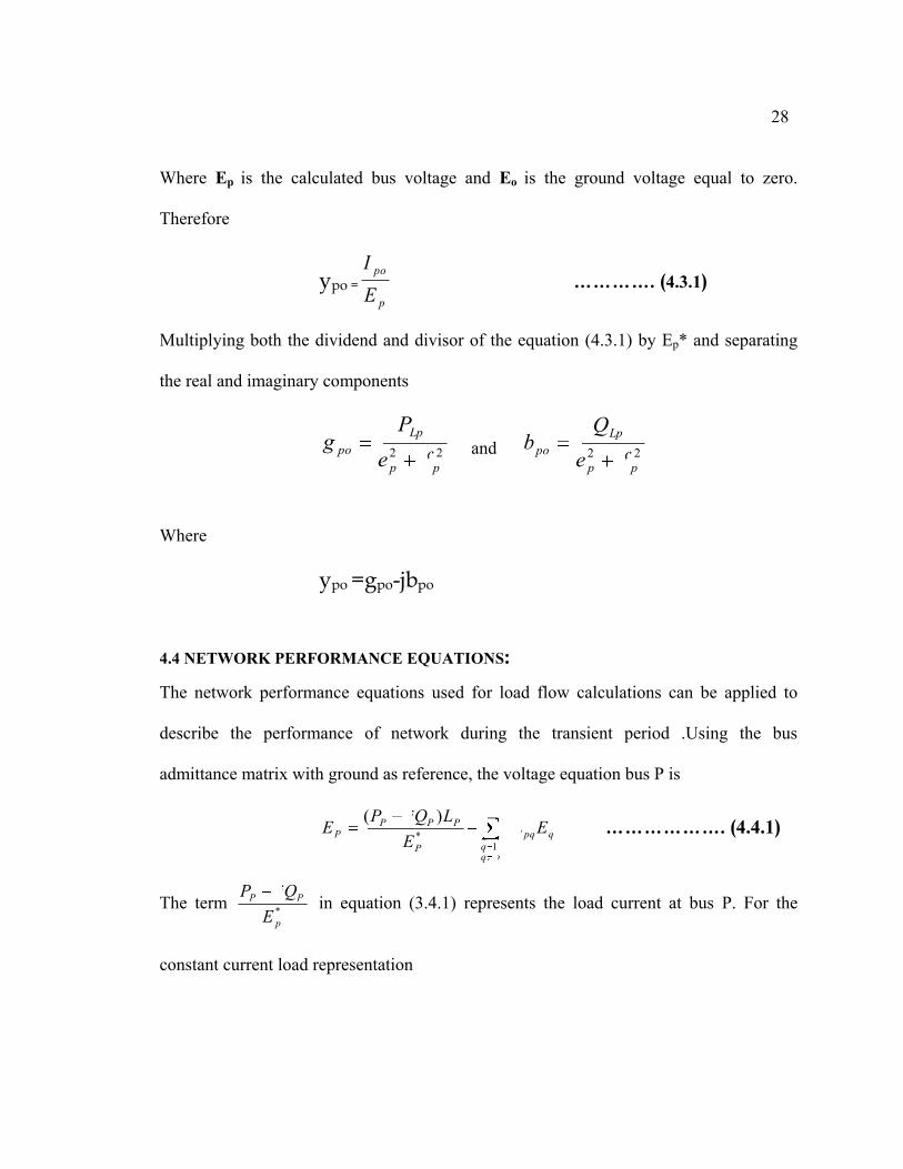
Where Ep is the calculated bus voltage and Eo is the ground voltage equal to zero.

Therefore

ypo =

p

po

E

I …………. (4.3.1)

Multiplying both the dividend and divisor of the equation (4.3.1) by Ep* and separating

the real and imaginary components

22

pp

Lp

pofe

Pg and 22

pp

Lp

pofe

Qb

Where

ypo =gpo-jbpo

4.4 NETWORK PERFORMANCE EQUATIONS:

The network performance equations used for load flow calculations can be applied to

describe the performance of network during the transient period .Using the bus

admittance matrix with ground as reference, the voltage equation bus P is

qpq

n

pqqP

PPPP ELY

E

LjQPE

1*

)( ………………. (4.4.1)

The term *

p

PP

E

jQP in equation (3.4.1) represents the load current at bus P. For the

constant current load representation

29

)()( * p

k

ppok

p

PP IE

jQP ………………. (4.4.2)

Where p is the power factor angle and k

p is the angle of voltage with respect to

reference. When the constant power is used to represent the load PPP LjQP )( will be

constant but the bus voltage pE will change every iteration. When the node at bus p is

represented by a static admittance to ground, the impressed current at the bus is zero and

therefore

*

)(

P

PPP

E

LjQP=0

In using equation (4.4.1) to describe the performance of the network for a transient

analysis, the parameters must be modified to include the effects of the equivalent

elements required to represent synchronous and induction machines and loads. The line

parameters pqYL must be modified for the new elements and an additional line parameter

must be calculated for each new network element. [1, 3, 26]

Let us consider the system shown in fig (4.2), which was used to illustrate the load flow

solution techniques.

30

The model has two machines and a load at each bus representing all loads as static

admittance to ground, the voltage equation for bus one is shown in Fig (4.2)

0104143132121 EYLEYLEYLEYLE

Where

11414

11313

11212

LYYL

LYYL

LYYL

The elements 12Y , 13Y and 14Y from the bus admittance matrix of the network are the

same as in load flow representation.

3 5

8

2

1

4

7 6

0

Network elements Elements representing machine and loads

Fig 4.2.1: Single line diagram of Power System for Transient analysis [1]

S

31

However,

11

1

1

YL

Where

1014131211 yyyyY

include the static admittance representing the load. Since E0 is zero, the line parameter

YL10 does not have to be calculated.

The voltage equation for bus 2 is

8286265251212 EYLEYLEYLEYLE

where bus 8 is a new bus. In this case the diagonal admittance elements for bus 2 is

282026252122 yyyyyY

where 20y is the static admittance representing the load and is the machine equivalent

admittance. The formulas for the Gauss-Siedal iterative solution of the network shown in

the above figure (4.2)

1

464

1

262

1

6

1

353

1

252

1

5

747646

1

141

1

4

535

1

131

1

3

828626525

1

121

1

2

414313212

1

1

KKK

KKK

KKK

KKK

KKKK

KKKK

EYLEYLE

EYLEYLE

EYLEYLEYLE

EYLEYLE

EYLEYLEYLEYLE

EYLEYLEYLE

The initial bus voltages are obtained from the load flow solution prior to the disturbance,

these voltages for the new buses 7 and 8 are obtained from the equivalent circuit

32

representing the machine. Subsequent voltages for the buses are calculated from the

differential equations describing the performance of the machines.[1,3,26]

During the iterative calculation the magnitudes and of the bus voltages behind the

machine equivalent admittances are held constant. If a three phase is simulated the

voltage of faulted bus is set to zero and held constant. If the bus impedance matrix is used

for a transient stability study, ground is usually taken as reference because all network

bus voltages, except at the faulted bus, change during the transient period. To eliminate

the need to modify the bus impedance matrix for a change in the reference bus, ground is

used also as reference in the prefault load flow calculation.[1,3,26]

When ground is used as reference for the load flow calculation and the loads are

represented solely as current sources, the bus impedance matrix will include only the

capacitor, reactor and the line charging elements to ground. In this case the bus

impedance matrix is ill conditioned and convergence of the solution is usually is not

obtained. On the other hand if the loads are represented solely as impedance to ground to

improve the convergence characteristic then these impedances and the bus impedance

matrix must be modified during the iterative solution for changes in bus voltages. To

overcome this difficulty only a portion of each bus load is represented as impedance to

ground. The remaining portion of the load can be represented as current source which

varies with the bus voltage so that the total bus current satisfies the scheduled load power.

33

After the load flow solution is obtained, the bus impedance matrix must be modified to

include the new network elements representing the machines and to account for the

changes in representation of loads. These modifications can be made by using the

algorithm described. Each element representing a machine is a branch to a new bus, and

each element representing a load change is a link to ground. [1,3,26]

The iteration formula for the performance of the network during the transient period

using ground as reference is

mn

q

qpq

K

P IZE1

1

……………… (4.4.3)

np ...........,.........3,2,1

Where n is the number of network buses, m is the number of buses behind the equivalent

machine impedances and bus f is the faulted bus. The current vector qI is composed of

load currents from either the constant currents or constant power representation and the

currents obtained from machine equivalent circuits.[1,3,26]

The application of the bus impedance matrix, only those rows and columns

corresponding to machines, constant power and constant current sources need to be

retained for the network solution. All rows and columns would have to be maintained,

P ≠ f (f is the fault bus)

34

however its system voltages and power flows are required during the transient

calculations. [1, 3, 26]

The procedures required using the bus impedance and admittance matrices and

representing each machine as a voltage behind the machine impedance is an application

of Thevinin’s theorem. An alternate method is to represent the machine as a current

source between the machine terminal bus and ground and in parallel with the machine

impedance. This is an application of Norton’s Theorem. This eliminates the need to

establish the additional bus behind the impedance of each machine. The machine currents

are calculated by using the internal machine voltages and the machine impedances. These

currents are held constant during network iterative solution. [1, 3, 26]

35

Chapter 5

MULTIMACHINE TRANSIENT STABILITY STUDY

5.1 Multi-Machine Transient Stability Studies:

The equal-area criterion cannot be used directly in systems where three or more machines

are represented. Although the physical phenomena observed to in the two machines

basically reflect that of the multi-machine case, nonetheless, the complexity of the

numerical computations increases with the number of machines considered in a transient

stability studies. When a multi-machine system operates under electro-mechanical

transient conditions, inter-machine oscillations occur between the machines through the

medium of the transmission system, which connects them. If any one machine could be

considered act alone as the single oscillating source, it would send into the inter-

connected system an electro-mechanical oscillation determined by its inertia and power a

typical frequency of such oscillation is of the order of 1 to 2 Hz and this is super-imposed

upon the nominal 50 Hz frequency of the system. When many machine rotors are

simultaneously under going transient oscillation, the swing cures will reflect the

combined presence of many such oscillations. Therefore, the transmission system

frequency is not unduly perturbed from nominal frequency, and the assumption is made

that the 50Hz network parameters are still applicable. [1, 2, 3, 26]

Aligned with such complexity in system modeling which evolve problems involving

large disturbances which do not allow the linearization process to be used and the non-

36

linear differential and algebraic equations must be solved by direct methods or by

iterative step by step procedures. These transient stability problems may be analyzed by

first swing stability studies, which are based on reasonably simple generated model

without representation of control systems. [1, 2, 3, 26]

5.2 Classical transient stability studies:

The classical model is used to study the transient stability of a power system for a period

of time during which the dynamic behavior of the system is largely dependent on the

stored energy in the rotating inertias. Usually the time period under study is the first

second following a system fault .If the machines of the system are found to remain in

synchronism with in the first second, the system is said to be stable. This is the simplest

model used in stability studies and requires minimum amount of data. [1, 2, 3, 26]

To ease the complexity system modeling and the computational burden the following

assumptions are made in developing the classical model are as follows: [26]

1) The mechanical power input to each machine remains constant during the entire

period of the swing curve computation.

2) Damping or asynchronous power is negligible.

3) Each machine may be represented by a constant transient reactance in series with

a constant transient voltage

37

4) The mechanical rotor angle of each machine coincides with the electrical phase

angle of the transient voltage.

5) All loads may be considered as shunt impedances to ground with values

determined by conditions prevailing immediately prior to the transient conditions.

The system stability model based on the assumptions is called the classical stability

model and studies which use this model, are called classical stability studies or first

swing stability studies. [1, 26]

This model is useful for stability analysis but is limited to the transients for only the

“First swing” or for periods on the order of one second. Assumption 2 can be improved

by assuming a linear damping characteristic. A damping torque Dω is frequently added to

the inertial torque in the swing equation. [1, 26]

The damping co-efficient D includes the various damping torque components, both

mechanical and electrical values of damping co-efficient. The modified study state model

of synchronous machine is shown in fig (5.1) for the purpose of transient stability

analysis as per the assumption three. The reactance1

dX is a direct transient reactance. The

constant voltage source || E determined from the initial conditions (i.e. pre

disturbance power flow conditions). [1, 26]

38

During the transient the magnitude of |E| is held constant with a variation of angle

is governed by

MG PPDM )( …………….(5.2.1)

Load representation can have a marked effect on stability results. The representation of

loads has constant impedances is usually made for simplicity based on assumption 5. This

assumption allows us to eliminate the algebraic network equations and reduce the system

of equations for the multi machine system to a system consisting of only differential

equations. [1, 26]

Fig 5.2: Representation of a synchronous machine by constant voltage behind transient reactance [1]

+

-

+

-

jx'd

Va

Id

E

39

5.3: Numerical Methods for Solution of Swing equation:

In general, methods of numerical integration employ a step-by-step process to determine

a series of values for each dependent variable corresponding to a selected set of values of

the independent variable. The usual procedure is to select values of the independent

variable at fixed intervals. The accuracy of a solution by numerical integration depends

both on the method chosen and the size of interval. In this project to solution differential

equations modified Euler’s method.[1]

5.3.1 Modified Euler method:

When a machine is represented by a voltage of constant magnitude back of transient

reactance, it is necessary to solve two first-order differential equation to obtain the

changes in the internal voltage angle δi and machine speed ωi. Thus for an m machine

problem where all machines are represented in the simplified manner, to is necessary to

solve 2m simultaneous differential equations. These equations are

fdi

dti

i 2)( …………… (5.3.1)

)(tqimi

i

i PPH

f

dt

d i=1, 2, 3. . . m

If no governor action is considered, Pmi remains constant and

Pmi=Pmi(0)

40

In the application of the modified Euler method the initial estimates of the internal

voltage angles and machine speeds at time t + Δt are obtained from

tdt

dt

ititti

10 ……………………….(5.3.2)

tdt

dt

ititti

10 i=1, 2, 3. . . m ……(5.3.3)

Where the derivatives are evaluated from equations (5.3.1) and teiP are the machine

powers at time t. when t = 0, the powers 0eiP are obtain from the network solution at the

instant after the disturbance occurs. Second estimates are obtained by evaluating the

derivatives at time t + Δt. This requires that initial estimates be determined from the

machine powers at time t + Δt. These powers are obtained by calculating new

component of the internal voltage from

00 cos ttiitti Ee …..………………. (5.3.4)

00 sin ttitti Ef ….……………….. (5.3.5)

Then the network solution is obtained holding fixed the voltages at the internal machine

buses. When there is a three-phase fault on bus f, the voltage Ef also is held fixed at zero.

41

With the calculated bus voltages and the internal voltages, machine terminal currents can

be calculated from

diai

tttittitttixjr

EEI1000

and machine power from

000 Re ttitttittei EIP

The second estimates for the internal voltage angles and machine speeds are obtained

from

tdt

d

dt

dtt

it

i

titti2

10

……… (5.3.6)

tdt

d

dt

dtt

it

i

titti2

11 i=1,2,3…m ...... (5.3.7)

Where

42

fdt

dttitt

i 20

)(

0

tteimi

i

tti PP

H

f

dt

d

The final voltages at time t + Δt for the internal machine buses are

11 cos ttiitti Ee ………. (5.3.8)

11 sin ttiitti Ef i=1, 2, 3… m ……... (5.3.9)

Then the network equations are solved again to obtain the final system voltages at time t

+ Δt. The bus voltages are used along with the internal voltages to obtain the machine

currents and powers and network power flows. The time is advanced by the Δt and a test

is made to determine if the switching operation is to be affected or the status of the

fault is to be changed. If an operation is scheduled, the appropriate changes are made in

network parameters or variables, or both. Then the network equations are solved to obtain

system conditions at the instant after the change occurs. In this calculation the internal

voltages are held fixed at the current values. Then estimates are obtained for the next time

43

increment. The process is repeated until t equals the maximum time maxT specified for

the study. [1,3]

The sequence of steps for transient analysis by the modified Euler method and the load

flow solution by the Gauss-Seidel iterative method using YBUS in flow chart. Shown also

are the main steps of the preliminary calculations. The procedure shown assumes that all

system loads are represented as fixed impedances to ground. [1,3]

When the effects of the saliency and the changes in field flux linkages are to be included

in the representation of the machines the following differential equations must be solved

simultaneously.[1,3]

fdt

dti

i 2

teimi

i

i PPH

f

dt

d ..................... (5.3.10)

Iifdi

doi

qiEE

Tdt

Ed 1 i=1, 2, 3...m

Again, if no governor action is considered, Pmi remains fixed and

0mimi PP

If the effects of the exciter control system are not included, Efdi remains constant and

44

0fdifdi EE

If each machine of the system is described by equation (5.3.10), 3m simultaneous

equations must be solved.

5.4: STATCOM in Power System:

To include the significant components in stability study it is necessary to represent the

controller design adequately to represent the mathematical model of a power system.

[21]

5.4.1 Synchronous generator and its Excitation System:

The synchronous generator is modeled through q-axis component of transient voltage and

electromechanical swing equation representing motion of the rotor. The internal voltage

equation of the generator is written as,

TIxxeEe

do

dddqfdq '

''.' 1])([ …………… (5.4.2.1)

where, .'

qe subscript d and q represents the direct and quadrature axis of the

machine, dx ,'

dx and '

doT are the d-axis synchronous reactance, transient reactance and open

circuit field constants, respectively. Id is the current along the d-axis and '

qe is the voltage

behind the transient reactance. [21]

45

Now the electromechanical swing equation is broken into two first order differential

equations and is written as,

][2

1.

Dem KPPH

…………………………… (5.4.2.2)

0

.

where, the electrical power output is,

qqdde IvIvP …………………………….. (5.4.2.3)

vd and vq are components of generator terminal voltage (Vt). Pm is the mechanical power

input. H is the inertia constant in seconds, (2H = M). 0 is the synchronous speed. [21]

The IEEE type ST is used for the voltage regulator excitation. The block diagram of the

excitation system is shown in Fig. 3.2.

Fig. 5.4.2.1: Block diagram of excitation system [21]

46

The dynamic model of the excitation system is,

.

)(1

tm

A

Afd

A

fd VVT

KE

TE ……………………. (5.4.2.4)

where, KA and TA are the gain and time constant of exciter, respectively. Vto represents

the steady state (reference) value of terminal voltage.[21]

47

Chapter 6

ALGORITHM AND FLOW CHART

6.1 Algorithm for Classical Transient stability study:

Step1: Read the bus data i.e. bus codes, impedance, line charging admittance and the

scheduled generation and loads of the given system.

Step2: The Y bus matrix is calculated from the lines, transformer, STATCOM data and

shunt element data and the load flow solution prior to the disturbance is calculated by

using Newton-Raphson iterative method.

Step 3: If there is any switching action we have to modify the system data first and also,

solve the network performance equations, calculate machine currents tiI and the

machine terminal powers tiP , tiQ for all buses by using the equations

(6.1.1),(6.1.2)and(6.1.3) respectively, otherwise go to step4

m

t

tpt

p

q

n

pq

k

qpq

k

qpq

k

p EYLEYLEYLE1

11

1 1

11 ………………. (6.1.1)

...,.........2,1 np

fp (When fault on bus f)

48

diai

tittixjr

EEI1

)( 1

…………… ………………… (6.1.2)

i=1, 2, 3…

titititi EIjQP ……….……………………… (6.1.3)

i=1, 2, 3… m

Step 4: Compute the inertial estimates of power angles, machine speeds and inertial

estimates of voltages behind machine impedances all of them at t + ∆t by using the

equations (5.3.2), (5.3.3), (5.3.4) and (5.3.5).

Step 5: Solve the network performance equations and calculate machine currents Iti and

calculate the machine terminal powers Pti and Qti for these machines by using equations

(6.1.1), (6.1.2)and(6.1.3).

Step 6: Calculate final estimates of power angles and machine speeds and also find the

estimates of voltages behind the machine impedance at t + ∆t by using the equations

(5.3.6), (5.3.7), (5.3.8) and (5.3.9), and solve the equation (6.1.1),(6.1.2)and(6.1.3).

Step 7: Advance the time t + ∆t to t and test for the time limit, if it is less than Tmax then

go to step3 otherwise print results.

49

6.2 Flow Chart for Modified Euler’s method [1]

NO

NO

YES

Start

Calculate load flow to

disturbances prior

Calculate load flow to

disturbances prior

Calculate machine currents Iti=ti

titi

E

jQP i=1, 2,., m

Calculate voltages behind machine equivalents

E'i(0) = Eti+raiIti+jx'diIti i =1, 2…m

Set time t=0

Is there a

switching

operation or

change in fault

condition?

Calculate initial estimates of power

angles and machine speeds at t+∆t

tdt

dt

i

titti )(

)1(

)(

)0(

)(

tdt

dt

i

titti )(

)1(

)(

)0(

)(

i=1, 2, 3... .m

Calculate initial estimates of voltages

behind machine impedances at t+ ∆t 0)0(

)( costtiitti Ee

00 sinttiitti

Ef

i=1, 2, 3….m

C

B

A

D

50

Calculate machine currents

Iti= (E'i-Eti ) air

1

jX'di

i=1, 2… m

Modify system data

B

E

C

D

G

Set j=0

Solve Network Performance equations

m

t

tpt

p

q

n

pq

k

qpq

k

qpq

k

p EYLEYLEYLE1

11

1 1

11

p =1, 2,…, n fp

Calculate machine terminal powers

Pti-jQti=ItiE*

ti

i=1, 2,…, m

Test j: 0

Test j: 1

Equal

Not equal

Equal

Not equal

Set j=1

C

Calculate final estimates of power angles

and machine speeds at t + ∆t

tdt

d

dt

dtt

it

i

titti2

1)1(

)(

tdt

d

dt

dtt

i

t

i

titti2

11

i=1, 2, 3 …m

F

51

Test for time

limit t: Tmax

Advance time t+ ∆t t

G

F

E

A

Calculate final estimates of voltage

Behind machine impedances and t+∆t

11

11

sin

cos

ttiitti

ttiitti

Ef

Ee

i=1, 2, 3….m

Set j=2

Print results

52

Chapter 7

RESULTS

7.1 Case Study (Stable case):

In this case the machines are represented by detailed models and loads are modeled as

constant admittances. The disturbances considered are three-phase faults at different

buses.

A two- generator, five bus system is considered in which a 3-phase fault is created on

machine-2,and this is cleared after 0.15sec.Numerical integration of the swing equation

are obtained with the help of digital computer by using modified Euler

’s method with a

time period of 1.0 sec. The swing curve is shown in fig (7.1) & (7.2).from that figures

system is found to be stable.

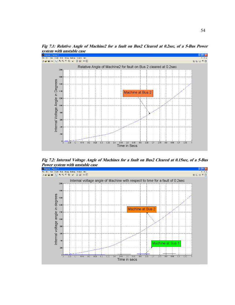
7.2 Case Study (Unstable case):

In this case the three-phase fault is created on machine-2, and the fault is cleared after

0.2 sec. Numerical integration of the swing equations are obtained with the help of digital

computer by using modified Euler’s method with a time period of 1.0 sec. and the swing

curve is shown in fig (7.3) & (7.4).from that figures system is found to be unstable.

From these two cases we can infer that, if the fault is cleared within 0.15 sec the system is

found to be stable and if clearance time is increased then the system is in unstable

condition which is evident from the simulated results (7.3) and (7.4).

53

Fig 7.1: Relative Angle of Machine2 for a fault on Bus2 Cleared at 0.15sec, of a 5-Bus Power system with Stable case

Fig 7.2: Internal Voltage Angle of Machines for a fault on Bus2 Cleared at 0.15sec, of a 5-Bus Power system with Stable case

54

Fig 7.1: Relative Angle of Machine2 for a fault on Bus2 Cleared at 0.2sec, of a 5-Bus Power system with unstable case

Fig 7.2: Internal Voltage Angle of Machines for a fault on Bus2 Cleared at 0.15sec, of a 5-Bus Power system with unstable case

55

Time in seconds

Relative rotor angles in degrees

12

0 7.24 0.05 14.51 0.1 32.18 0.15 50.77 0.2 56.41 0.25 47.9 0.3 27.08 0.35 -0.59 0.4 -25.61 0.45 -38.51 0.5 -34.86 0.55 -16.87 0.6 7.87 0.65 29.92 0.7 42.44 0.75 42.69 0.8 31.14 0.85 11.2 0.9 -10.49 0.95 -25.82

1 -29.06

Table 7.1: Simulation results for fault on bus-2 cleared at 0.15 sec, for a 5-bus system with stable case (Classical transient stability)

56

Time in seconds

Internal voltage angles

1 in degrees 2 in degrees

0 12.15 19.39

0.05 12 26.51

0.1 12.26 44.44

0.15 12.82 63.59

0.2 13.55 69.96

0.25 14.48 62.39

0.3 15.62 42.69

0.35 16.85 16.26

0.4 18.01 -7.61

0.45 18.9 -19.6

0.5 19.42 -15.44

0.55 19.52 2.64

0.6 19.26 27.13

0.65 18.78 48.7

0.7 18.25 60.69

0.75 17.81 60.5

0.8 17.51 48.65

0.85 17.33 28.53

0.9 17.15 6.66

0.95 16.83 -8.99

1 16.23 -12.83

Table 7.2: Simulation results for fault on bus-2 cleared at 0.15 sec, for a 5-bus system with stable case

(Classical transient stability)

57

Time in seconds

Relative rotor angles

in degrees

12

0 7.24

0.05 14.51

0.1 32.18

0.15 60.25

0.2 98.27

0.25 132.79

0.3 163.65

0.35 202.72

0.4 263.5

0.45 350.43

0.5 441.5

0.55 520.97

0.6 607.46

0.65 718.5

0.7 832.04

0.75 940.06

0.8 1068.71

0.85 1202.87

0.9 1335.38

0.95 1487.89

1 1636.94

Table 7.3: Simulation results for fault on bus-2 cleared at 0.2 sec, for a 5-bus system with unstable case (Classical transient stability)

58

Time in

seconds

Internal voltage angles

1 in degrees 1 in degrees

0 12.15 19.39

0.05 12 26.51

0.1 12.26 44.44

0.15 12.92 73.17

0.2 13.99 112.26

0.25 15.48 148.27

0.3 17.36 181.01

0.35 19.52 222.23

0.4 21.73 285.23

0.45 23.67 374.1

0.5 25.32 466.82

0.55 27.13 548.1

0.6 29.18 636.64

0.65 31.06 749.57

0.7 32.73 864.77

0.75 34.63 974.69

0.8 36.5 1105.21

0.85 38.16 1241.03

0.9 40.02 1375.4

0.95 41.72 1529.61

1 43.42 1680.36

Table 7.4: Simulation results for fault on bus-2 cleared at 0.2 sec, for a 5-bus system with unstable case (Classical transient stability)

59

Chapter 8

CONCLUSION

In this work, an attempt has been made to study the Load flow and the transient stability

of the multi-machine system using FACT Devices. The Load flow studies are carried out

with and without STATCOM and Newton-Raphson method is used in Load flow. The

results indicated an overall improvement network voltage profile. And in general more

reactive Power was available in the network with STATCOM installed than without and

the generator2 increases its share of reactive power absorption when compared with the

base case.

In Transient stability study the step-by-step methods are used and the results have been

simulated using MATLAB. The classical study has been carried out on the same five bus

power system constituting two generators, a STATCOM and four loads. Modified Euler’s

method has been applied to the solution of the differential equations in transient stability

studies. . The results have been tabulated and corresponding swing curves are plotted.

From the Stability study, we can conclude that if the fault is cleared in 0.15 sec during a

study period of 1.0 sec, the system is found to be in stable condition, and if the fault

clearing time is 0.2 sec the system is found to be in unstable condition. The transient

stability can be further increased by temporarily increasing the voltage above the

60

regulation reference for the duration of the first acceleration of the machine. The voltage

increased above its nominal value will increase the electric power transmitted and thus,

will also increase the deceleration of the machine and thereby there will be an attainable

increase in transient stability margin when compared to a system without STATCOM.

The results of this book are compared with the results from G.W.Stagg and A.H.E.L –

abiad “Computer Methods in power systems” and can significantly point that the stability

increased by 0.05secs with Installtion of STATCOM in the system. This proves that

STATCOM improves the transient stability of a System.

61

Appendix A

System data

A.1: 5-Bus system data

Number of buses: 5

Number of generators: 2

Number of lines: 7

Number of tap changing transformers: 0

Slack bus number: 1

Number of shunts: 0

Base in MVA: 100

6

1 3 4

5 2

7

S

Fig A.1 Single line diagram representation of 5 bus system for transient stability

calculation

62

Convergence factor: 0.0001

Acceleration factor: 1.4

Table A.1: Impedance and line charging admittance for a 5-Bus system

Starting

bus

Ending

bus Impedance

Line charging

Admittance

1

1

2

2

2

3

4

2

3

3

4

5

4

5

0.02

0.08

0.06

0.06

0.04

0.01

0.08

0.06

0.24

0.18

0.18

0.12

0.03

0.24

0.0

0.0

0.0

0.0

0.0

0.0

0.0

0.030

0.025

0.020

0.020

0.015

0.010

0.025

63

TableA.2: Scheduled generation and loads and specified bus voltages for a

5-Bus system

Bus number Generation Load Bus voltages

MW MVAR MW MVAR

1

2

3

4

5

0.00

40.00

0.00

0.00

0.00

0.00

30.00

0.00

0.00

0.00

0.00

20.00

45.00

40.00

60.00

0.00

10.00

15.00

5.00

10.00

1.06

1.00

1.00

1.00

1.00

0.0

0.0

0.0

0.0

0.0

Table A. 3: Inertia constants, direct axis transient reactance

M/C number

Inertia constant H

Direct axis transient reactance

1 2

50.0 1.0

0.25 1.50

64

Table A. 4: Static Synchronous Compensator Data (STATCOM)

Parameters

Values in

(p.u)

Converter's reactance 10

Target Voltage Magnitude 1

Target Active power Flow 0

Target Reactive Power Flow 0

Initial Source Voltage 1

Initial Source Angle 0

Lower limit of Voltage magnitude 1.1

Upper limit of Voltage Magnitude 0.9

65

BIBLIOGRAPHY

[1] G.W.Stagg and A.H.EL-abaid, “Computer methods in power systems (New York

hills, 1968).

[2] P.K. Padiyar, “Power system stability and control” EPRI Power system series 1994.

[3] P.M. Anderson and A.A.Fouad, “Power system control and stability”, Iowa state

university press, 1980.

[4] Kimbark, “Power system stability”, vol. 1

[5] Y.N. YU, “Electric power system dynamics”, Academic press 1983.

[6] E.Lerch, D.Porh and L.XU, “Advanced SVC control for damping power system

oscillations”, 1991.

[7] N.Mithulananthan, C.A Canizares, J.Reeve and G.J.Rogers, “Comparison of PSS,

SVC and STATCOM controllers for damping power system oscillations”. IEEE

transactions on power systems, vol. 18, no.2, pp 786-792, May 2003.

[8] A.M.Stankovic, P.C.Stefanov, G.Tadnor and D.J.Somajic, “Dissipativity as a unifying

control design framework for suppression of low frequency oscillations in power

systems”. IEEE transaction on power system vol.14, no.1, pp 192-199 February 1999.

[9] J.Chen, J.V.Milanovic, F.M.Huges, “Selection of auxiliary input signal and location

of SVC for damping electro-mechanical oscillations”. IEEE transactions on power

system vol. pp 623-627 2001.

66

[10] D.N.Koterev, C.W.Taylor and W.A.Mittlestadt, “Model validation for August 10,

1996 WSCC system outage”. IEEE transactions on power systems vol. 14, pp 967- 979,

August 1999.

[11] N.mithlananthan and S.C.Srivastva, “Investigation of voltage collapse in srilanka’s

power system network”. In proc EMPD Singapore, pp 47-52, March 1995, IEEE catalog

98 EX 137.

[12] Demello, P.J.Molan, T.F.Laskowski, J udrill, “Co-ordinated application of

stabilizers in multi-machine systems”. IEEE transaction on PAS, vol. PAS -99, pp 892

902, 1980.

[13] Demello and C.Concordia, “Concepts of synchronous machine stability as affected

by Excitation control”. IEEE trans power APP and systems, vol. PAS 103, no 8, pp 1983-

1989, 1984.

[14] N.G.Hingoroni, “Flexible AC transmission system”. Fifth IEE international

conference on AC and DC transmission (IEE-pub. no 345), pp 1-7 September 1991.

[15] N.G.Hingoroni, “Flexible AC transmission systems”, IEEE spectrum (40-45) April

1993.

[16] N.G.Hingoroni, “FACTS technology and opportunities IEEE colloquim”. (Digest

no. 1994/OCS) “FACTS the key to increased utilization of power system”, pp 4/1- 4/10,

Jan 1994.

67

[17] M.F.Kandlawala, “Investigation of dynamic behavior of power system installed with

STATCOM”, A thesis submitted to university of King Fahd University of Petroleum and

Minerals, December 2001.

[18] Laszlo Gyugi, “converter based facts controller”, IEE colloquium on FACTS pages

1-11, November 23, 1998.

[19] M.F.Kandlawala and A.H.M.A.Rahim, “Power system dynamic performance with

STATCOM controller”. 8th annual IEEE technical exchange meeting, April 2001.

[20] L.O.Mak, Y.X.Ni and C.M.Shen, “STATCOM with fuzzy controller for

interconnected power systems”, Electric power system research, August 1999, pp 87-95.

[21] Syed Faizullah Faisal “Damping Enhancement of Multi-Machine Power System

through STATCOM Control” King Fahd University of Petroleum & Minerals, Master’s

Thesis, March 2005

[22] Acha, C., Fuerte-Esquivel, C. R., Ambriz-Perez, H. and Angeles-Camacho, C.;

“FACTS. Modeling and Simulation in Power Networks”, John Wiley & Sons, 2004.

[23] Kalyan K.Sen, “STATCOM- Static Synchronous Compensator: Theory, Modeling &

Applications” IEEE Transaction on power systems, 1988.

[24] Douglas J.Gotham, G.J.Heydt “POWER FLOW CONTROL & POWER FLOW

STUDIES WITH FACTS DEVICES”, IEEE Transactions on Power Systems. Vol.13,

No.1, February, 1998

68

[25] T.J. Overbye and D. Brown. “Use of FACTS Devices for Power System Stability

Enhancement”, Proceedings of the IEEE 36th

Midwest Symposium on Circuits and

Systems, USA, 1993, Vol.2, pp.1019-1022.

[26] William D.Stevenson, Jr.” Elements of power system analysis” Fourth edition, Mc

Graw Hill book company.

[27] Proposed terms and definitions for flexible AC transmission system(FACTS), IEEE

Transactions on Power Delivery, Volume 12, Issue 4, October 1997, pp. 1848–1853.

[28] W.Breuer, D.Povh, D. Retzmann, E.Teltsch, XLei “Role of HVDC and FACTS in

future Power systems” CEPSI 2004 Shanghai

[29] Dussan povh Siemens AG “Modeling of FACTS in Power system Studies” IEEE

[30] Dr.L.Gyugyi, FIEEE “Unified power-flow control concept for Flexible AC

transmission systems”

[31] S.Ward, T.Dahlin, W. Higinbotham “Improving Reliability for Power system

protection” IEEE

[32] N.G Hingorani G. Gyugyi Lazlo “ Understanding FACTS: Concepts & technology

of flexible AC Transmission Systems” ISBN 0-7803-3455-8

[33]Tariq MASOOD.ch, Dr. Abdel-Aty Edris.Pro. Dr. RK Aggarwal “Static synchronous

Compensator (STATCOM) modeling and analysis Techniques by Matlab & SAT/FAT

Acceptance tests in the light of Commisioning & Installation Scenarios.” PSC 2006

[34] L.Kirschner, D.Retzman, G.Thumm Siemens AG, Germany “Benefits of FACTS for

Power System Enhancement” IEEE

69

[35] Gregory Reed, John Paserba and Peter Salavantis “The FACTS resolving

Transmission gridlock” IEEE Power & Energy magazine 1540 -7977 © 2003 IEEE

[36] University of Zielona Gora “ Power Electronics Arrangements in distributed

Systems” Institute of Electrical Engineering.

[37] P.Bhavani Shankar and Ch.Sai Babu “ Transient stability Enhancement of Power

system using STATCOM” International Journal Of Electric and Power engineering

ISSN:1990-7958 © Medwell Journals,2008

[38] T.J. Overbye and D. Brown. “Use of FACTS Devices for Power System Stability

Enhancement”, Proceedings of the IEEE 36th

Midwest Symposium on Circuits and

Systems, USA, 1993, Vol.2, pp.1019-1022.

[39] D P Kothari & I J Nagrath “ Modern power System Analysis” Tata McGraw Hills

2003 ISBN 0-07-049489-4.

[40] C. L .Wadhwa “Electrical power systems” ISBN : 81-224-1272-6

[41] Aditya Jayam Prabhakar “Application of STATCOM for improved Dynamic

Performance of Wind farms in a Power Grid” Missouri University of Science and

technology . Master’s Thesis 2008.

[42] Juan M Ramirez and J.L. Murillo Perez “ Application of Three-Phase STATCOM in

Voltage Stability” Center of research and Advanced studies, National polytechnic

Institute.